Quasinormal modes and greybody factor of a Lorentz-violating black hole

Abstract

Recently, a static spherically symmetric black hole solution was found in gravity nonminimally coupled a background Kalb-Ramond field. The Lorentz symmetry is spontaneously broken when the Kalb-Ramond field has a nonvanishing vacuum expectation value. In this work, we focus on the quasinormal modes and greybody factor of this black hole. The master equations for the perturbed scalar field, electromagnetic field, and gravitational field can be written into a uniform form. We use three methods to solve the quasinormal frequencies in the frequency domain. The results agree well with each other. The time evolution of a Gaussian wave packet is studied. The quasinormal frequencies fitted from the time evolution data agree well with that of frequency domain. The greybody factor is calculated by Wentzel-Kramers-Brillouin (WKB) method. The effect of the Lorentz-violating parameter on the quasinormal modes and greybody factor are also studied.

I Introduction

Lorentz symmetry is a fundamental concept in modern physics. It states that all physical laws are same in all inertial frames. Although Lorentz symmetry has been thought to be very important and has been tested by a lot of experiments and observations, it also can be violated in some gravity theories, for example, Einstein-æther theory Jacobson:2000xp , Horava-Lifshitz gravity Horava:2009uw , $f(T)$ gravity Bengochea:2008gz , or in some high energy scale, such as string theory Kostelecky:1988zi and loop quantum gravity Alfaro:2001rb . One of the frameworks for the Lorentz violating theories is the Standard-Model-Extension Kostelecky:2003fs . Different from the explicitly broken Lorentz symmetry theories, in this framework, the Lagrangian density is Lorentz invariant, but the ground state of the system will not. This can be achieved by some background field acquiring a nonzero vacuum expectation value.

One of the famous theories is the bumblebee gravity Kostelecky:1989jw ; Kostelecky:1989jp ; Bailey:2006fd ; Bluhm:2008yt . A vector field named as the bumblebee field with a nonzero vacuum expectation value selects a specific direction, this will break the local particle Lorentz symmetry. The bumblebee model has been studied widely. A static spherical symmetric black hole solution was found by Casana et al. in Ref. Casana:2017jkc . Then it was generalized to (anti) de Sitter cases Maluf:2020kgf . Two families of static spherical black hole solutions were obtained by investigating the background bumblebee field with a non-vanishing temporal component or radial component Xu:2022frb . The rotating bumblebee black holes were studied in Refs. Ding:2019mal ; Ding:2020kfr . A static spherical black hole solution with a global monopole was proposed in Ref. Gullu:2020qzu . Other black hole solutions were also studied Ding:2021iwv ; Jha:2020pvk ; Ding:2022qcy . The thermodynamic properties and observation effects of the bumblebee black holes were investigated in Refs. Mai:2023ggs ; Wang:2021irh ; Chen:2023cjd ; Zhang:2023wwk ; Lin:2023foj ; Wang:2021gtd .

Instead the bumblebee field, the local particle Lorentz symmetry can also be broken by a rank-two antisymmetric tensor field, named as the Kalb-Ramond (KR) field  Altschul:2009ae . The KR field can emerge from string theory Kalb:1974yc . When the KR field has a nonzero vacuum expectation value and couples to gravity, the Lorentz symmetry can be broken spontaneously. Under the nonzero vacuum expectation value, a static and spherically symmetric solution was constructed in Ref. Lessa:2019bgi . Recently, a new class of solutions with and without the cosmological constant were proposed by Yang et al. in Ref. Yang:2023wtu . The shadow and the quasinormal modes (QNMs) of this black hole were studied Filho:2023ycx .

The detection of the gravitational waves by Laser Interferometer Gravitational-Wave Observatory (LIGO) and Virgo LIGOScientific:2016aoc and the first picture of the black hole by Event Horizon Telescope (EHT) EventHorizonTelescope:2019dse label that we have entered the multi-messenger astronomy. For the gravitational waves of a binary black hole merger system, there are three parts: inspiral, merger, and ringdown. It is believed that the gravitational waves in the ringdown stage are dominated by the QNMs Berti:2007dg . The QNMs are characteristic modes of dissipative systems. Different from the normal modes, the QNMs do not form a complete set Nollert:1998ys . The real parts of the quasinormal frequencies (QNFs) are the oscillation frequencies of the perturbation, and the imaginary parts are related to the decay time. The QNMs of the gravitational field can only depend on the parameter of the black hole, so it can be used to infer the mass and angular momentum of a black hole, and further to test the no-hair theorem Echeverria:1989hg ; Berti:2005ys ; Berti:2007zu ; Isi:2019aib . In addition, the ultracompact objects without event horizon could have echo signals, which could be used to test the existence of event horizons Cardoso:2016rao ; Cardoso:2019rvt ; Cardoso:2017cqb . Recently, it was found that the spectrum of the QNMs is unstable under the perturbation of the effective potential Jaramillo:2020tuu ; Cheung:2021bol . The time domain observations and the corresponding Regge Poles were studied in Refs Berti:2022xfj ; Torres:2023nqg . The QNMs in modified gravity theories were widely studied in Refs. Guo:2021enm ; Cardoso:2020nst ; Guo:2022rms ; Yang:2023gas ; Guo:2023vmc ; Li:2021ngc . Besides, the QNMs in brane world models were also studied in Refs. Seahra:2005wk ; Tan:2022vfe .

Another important concept for a black hole perturbation system is the greybody factor, which describes the transmission probability of an outgoing wave reach to infinity or an incoming wave to be absorbed by the black hole Konoplya:2019ppy ; Cardoso:2005vb ; Dey:2018cws . The greybody factor can describe the information of the near horizon regions of a black hole Kanti:2002nr . It can be used to evaluate the Hawking radiation energy emission Hawking:1975vcx . Recently, it was pointed out that the ringdown signal after an extreme mass ratio merger can be modelled by the greybody factor Oshita:2023cjz .

In this paper we want to study the QNMs and greybody factor of the scalar field, electromagnetic field and gravitational field in the background of the Lorentz-violating black hole in gravity nonminimally coupled a background Kalb-Ramond field. This paper is organized as follows. In Sec. II, we review the black hole solution briefly and give the master equations for the perturbed fields. In Sec. III, we solve the QNFs with three different methods, and study the effect of the Lorentz-violating parameter on the QNMs. In Sec. IV, we calculate the greybody factor with the Wentzel-Kramers-Brillouin (WKB) method. The conclusions are given in Sec. V.

II Background and perturbation equations

In this section we review the Lorentz-violating black hole briefly and derive the perturbed master equations for the scalar field, electromagnetic field, and gravitational field. The starting point is the following Einstein-Hilbert action coupled with a self-interacting KR field non-minimally Altschul:2009ae ; Lessa:2019bgi

$$S=\frac{1}{2\kappa}\int d^{4}x\sqrt{-g}\left[R-\frac{1}{6}H^{\mu\nu\rho}H_{\mu\nu\rho}-V(B^{\mu\nu}B_{\mu\nu}\pm b^{2})+\xi B^{\rho\mu}B^{\nu}_{\mu}R_{\rho\nu}\right]+\int d^{4}x\sqrt{-g}\mathcal{L}_{M},$$ (1)

where $\kappa$ is related to the Newtonian constant $G$ through $\kappa=8\pi G$, $\xi$ is the coupling constant between the KR field and the gravity. The field strength of the KR field is defined as $H_{\mu\nu\rho}\equiv\partial_{[\mu}B_{\nu\rho]}$. The key point is the nonvanishing vacuum expectation value (VEV) for the KR field, $\langle B_{\mu\nu}\rangle=b_{\mu\nu}$, and $b^{\mu\nu}b_{\mu\nu}=\mp b^{2}$. The sign $\pm$ in the potential $V$ is to ensure that the constant $b^{2}$ is a positive number Altschul:2009ae ; Kalb:1974yc ; Bluhm:2007bd . Due to the vacuum condensation, the gauge invariance of the KR field is spontaneously broken. Because the KR field is nonminimally coupled to the gravity, the spontaneous symmetry breaking could lead to the violation of local Lorentz symmetry. Similar to the Maxwell field, the KR field could be decomposed to a pseudo-electric and a pseudo-magnetic field. Assuming that only the pseudo-electric nonvanishing, the KR field strength will vanish, i.e., $H_{\lambda\mu\nu}=0$. Under the VEV configuration, the field equation could be written as

$$R_{\mu\nu} = V^{\prime}(2b_{\mu\alpha}b_{\nu}^{\alpha}+b^{2}g_{\mu\nu})+\xi\Big{[}g_{\mu\nu}b^{\alpha\gamma}b^{\beta}_{\gamma}R_{\alpha\beta}-b^{\alpha}_{\mu}b^{\beta}_{\nu}R_{\alpha\beta}-b^{\alpha\beta}b_{\mu\beta}R_{\nu\alpha}-b^{\alpha\beta}b_{\nu\beta}R_{\mu\alpha}$$ (2)

$$+ \frac{1}{2}\nabla_{\alpha}\nabla_{\mu}(b^{\alpha\beta}b_{\nu\beta})+\frac{1}{2}\nabla_{\alpha}\nabla_{\nu}(b^{\alpha\beta}b_{\mu\beta})-\frac{1}{2}\nabla^{\alpha}\nabla_{\alpha}(b_{\mu}^{\gamma}b_{\nu\gamma})\Big{]},$$

where the prime denotes the derivative with respect to the corresponding argument. Under the assumption that the VEV locates at the minimum of the potential, that is $V^{\prime}=0$, a Schwarzschild-like black hole solution in the theory is obtained Yang:2023wtu

$$ds^{2}=-f(r)dt^{2}+\frac{dr^{2}}{f(r)}+r^{2}d\theta^{2}+r^{2}\sin^{2}\theta d\phi^{2},$$ (3)

where $f(r)=\frac{1}{1-\gamma}-\frac{2M}{r}$ and $M$ is the Komar mass. The parameter $\gamma$ is dimensionless which is defined as $\gamma\equiv\xi b^{2}/2$. The Lorentz symmetry violation effect caused by the nonvanishing VEV of the KR field is characterized by the parameter $\gamma$. The event horizon locates at $r_{h}=2(1-\gamma)M$, which is different from the Schwarzschild black hole. Note that, in the limit $r\rightarrow\infty$ the Kretschmann scalar $R^{\alpha\beta\mu\nu}R_{\alpha\beta\mu\nu}$ is nonvanishing, which shows that the background spacetime is not asymptotically Minkowski. That means the Lorentz-violating effect cannot be removed by coordinate transformation. The solutions with the presence of cosmological constant were also obtained in Ref. Yang:2023wtu .

With this background spacetime, we would like to study the scattering wave of a perturbed field $\Psi^{s}$, where $s$ is the spin of the perturbed field, i.e., $s=0,\pm 1,\pm 2$ correspond to the scalar field, odd parity electromagnetic field, and odd parity gravitational field, respectively. The variable decomposition can be done with the help of the spherical harmonics, vectorial harmonics, and tensorial harmonics Edmonds ; Regge . The perturbed field equation for the radial part in the tortoise coordinate can be written as

$$\frac{d^{2}}{dr_{*}^{2}}\Psi^{s}+(\omega^{2}-V_{eff}^{s})\Psi^{s}=0,$$ (4)

where the tortoise coordinate is defined as $dr_{*}=\frac{dr}{f(r)}$. The effective potentials for the scalar field and electromagnetic field are

$$V_{eff}^{s}=\left\{\begin{array}[]{ll}f(r)\left(\frac{l(l+1)}{r^{2}}+(1-s^{2})\frac{2M}{r^{3}}\right)&\textrm{for the scalar field and electric field,}\\ f(r)\left(\frac{l(l+1)}{r^{2}}-\frac{2\gamma^{2}}{r^{2}(1-\gamma)^{2}}-\frac{6M}{r^{3}}\right)&\textrm{for the gravitational field.}\end{array}\right.$$

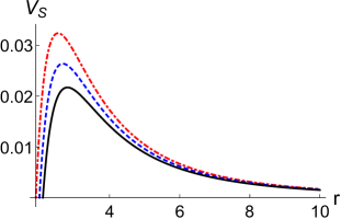
(a)

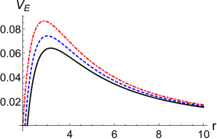
(b)

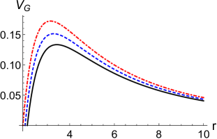
(c)

Figure 1: The effective potentials for different perturbed fields. The mass $M$ is set to $M=1$, and the Lorentz violating parameter $\gamma$ is set to $\gamma=-0.05$ (the black lines), $\gamma=0$ (the blue dots), and $\gamma=0.05$ (the red dashed dots). (a) The effective potential for the scalar field and $l=0$. (b) The effective potential for the Maxwell field and $l=1$. (c) The effective potential for the gravitational field and $l=2$.

The plots for the effective potentials for the three perturbed fields are shown in Fig. 1. From this figure we can see that, the effect of the parameter $\gamma$ on the effective potentials for the three perturbed fields are the same, that is the heights of the potentials increase with $\gamma$.

III Quasinormal mode frequencies

In this section, we will solve the master equation (4) to obtain the QNFs with three different methods, the continued fraction method Leaver1985 , the direct integration method Pani:2013pma , and the WKB method Konoplya:2003ii . Hereafter,we will set the mass $M=1$ in this paper. The boundary condition for this problem is

$$\Psi^{s} \sim e^{-i\omega r_{*}},~{}~{}~{}~{}~{}~{}r_{*}\rightarrow-\infty,$$

$$\Psi^{s} \sim e^{i\omega r_{*}},~{}~{}~{}~{}~{}~{}~{}~{}r_{*}\rightarrow+\infty,$$ (5)

which is only an ingoing wave at the horizon and only an outgoing wave at infinity.

Continued fraction method The continued fraction method proposed by Leaver Leaver1985 is the most exact method to solve QNFs of a black hole. The wave function satisfying the boundary (5) could be written as

$$\Psi^{s}=(r-2\eta)^{-2i\omega\eta^{2}}r^{4i\omega\eta^{2}}e^{i\eta\omega(r-2\eta)}\sum_{n=0}a_{n}\frac{(r-2\eta)^{n}}{r^{n}},$$ (6)

where $a_{n}$ is the expansion coefficient, and $\eta\equiv 1-\gamma$. Substituting this into the master equation (4), a three-term recurrence relation can be obtained:

$$\alpha_{0}a_{1}+\beta_{0}a_{0} = 0,$$ (7)

$$\alpha_{n}a_{n+1}+\beta_{n}a_{n}+\delta_{n}a_{n-1} = 0,~{}~{}~{}~{}~{}~{}n=1,2\ldots$$ (8)

where the recurrence coefficients $\alpha_{n}$, $\beta_{n}$, and $\gamma_{n}$ are functions of $n$ and the parameters of the black hole:

$$\alpha_{n}=(n+1)(n+1-4i\eta^{2}\omega),$$ (9)

$$\beta_{n}=\left\{\begin{array}[]{ll}-1-\eta l(l+1)-2n-2n^{2}+s^{2}+32\eta^{4}\omega^{2}+8i\eta^{2}(\omega+2n\omega)&\textrm{for the scalar field and electric field,}\\ -1+\frac{2}{\eta}-\eta(-2+l+l^{2})-2n-2n^{2}+32a^{4}\omega^{2}+8i\eta^{2}(\omega+2n\omega)&\textrm{for the gravitational field.}\end{array}\right.$$

$$\delta_{n}=\left\{\begin{array}[]{ll}(n-1)^{2}-s^{2}+(n-1)(2-8i\eta^{2}\omega)-(i+4a^{2}\omega)^{2}&\textrm{for the scalar field and electric field,}\\ -4+n^{2}-8i\eta^{2}n\omega-16\eta^{4}\omega^{2}&\textrm{for the gravitational field.}\end{array}\right.$$

From Eq. (7) we can obtain

$$\frac{a_{1}}{a_{0}}=-\frac{\beta_{0}}{\alpha_{0}}.$$ (10)

On the other hand, from the three-term recurrence relation (8) we can obtain a continued fraction

$$\frac{a_{1}}{a_{0}}=\frac{-\delta_{1}}{\beta_{1}-\frac{\alpha_{1}\delta_{2}}{\beta_{2}-\frac{\alpha_{2}\delta_{3}}{\beta_{3}-\cdots}}}$$ (11)

which can be rewritten into a usual notation as

$$\frac{a_{1}}{a_{0}}=\frac{-\delta_{1}}{\beta_{1}-}\frac{\alpha_{1}\delta_{2}}{\beta_{2}-}\frac{\alpha_{2}\delta_{3}}{\beta_{3}-}\cdots$$ (12)

Comparing Eqs. (10) and (12), we can obtain the QNFs by solving the following relation

$$0=\beta_{0}-\frac{\alpha_{0}\delta_{1}}{\beta_{1}-}\frac{\alpha_{1}\delta_{2}}{\beta_{2}-}\frac{\alpha_{2}\delta_{3}}{\beta_{3}-}\cdots$$ (13)

Direct integration Another useful method to solve the fundamental and lower overtone QNFs is the direct integration method Pani:2013pma . First we should expand the wave function $\Psi^{s}$ at horizon and infinity to satisfy the boundary condition (5). Then we integrate the master equation (4) from both horizon and infinity and match them at a certain point. By imposing the wave functions should be continued and their first derivatives are also continued, the eigenvalues, i.e., the QNFs can be solved.

WKB method The basic idea of the WKB method is to match the asymptotic WKB solutions at the two boundaries (horizon and infinity) with the Taylor expansion near the peak of the potential through two turning points. For 6th order WKB method, the QNFs can be evaluated through Konoplya:2003ii

$$\frac{i(\omega_{n}^{2}-V_{0})}{\sqrt{-2V_{0}^{\prime\prime}}}+\sum_{j=2}^{6}\Lambda_{j}=n+\frac{1}{2},$$ (14)

where $V_{0}$ and $V_{0}^{\prime\prime}$ represent the peak value of the effective potential and the second derivative with respect to the tortoise coordinate at the peak value of the effective potential, respectively. The correction terms $\Lambda_{j}$ depend on the peak value of the potential and higher-order derivatives of the peak value Konoplya:2003ii ; Iyer:1986np ; Konoplya:2002zu .

$\gamma$	$n$	Direct Integration	Continued Fraction	WKB
		$\omega_{\text{R}}M$    $\omega_{\text{I}}M$	$\omega_{\text{R}}M$    $\omega_{\text{I}}M$	$\omega_{\text{R}}M$     $\omega_{\text{I}}M$
-0.05	0	0.101906    -0.094972	0.100185    -0.095142	0.100198    -0.091442
	1	0.078359    -0.368925	0.077706    -0.316039	0.080754    -0.312488
0	0	0.111714    -0.104218	0.110454    -0.104894	0.110464    -0.100819
	1	0.085238    -0.346023	0.085671    -0.348433	0.089023    -0.344552
0.05	0	0.123085    -0.115260	0.122387    -0.116227	0.122401    -0.111708
	1	0.094612    -0.389441	0.094927    -0.386075	0.098647    -0.381752

Table 1: The fundamental and first overtone QNFs of the scalar field for different values of $\gamma$ through three methods. The angular number $l$ is set to $l=0$.

$\gamma$	$n$	Direct Integration	Continued Fraction	WKB
		$\omega_{\text{R}}M$    $\omega_{\text{I}}M$	$\omega_{\text{R}}M$    $\omega_{\text{I}}M$	$\omega_{\text{R}}M$     $\omega_{\text{I}}M$
-0.05	0	0.231800    -0.084056	0.231800    -0.084056	0.231744    -0.084175
	1	0.199991    -0.269997	0.201756    -0.266227	0.201581    -0.266583
0	0	0.248263    -0.092488	0.248263    -0.092488	0.248191    -0.092637
	1	0.209938    -0.290036	0.214515    -0.293668	0.214295    -0.294118
0.05	0	0.266761    -0.102253	0.266761    -0.102252	0.266668    -0.102443
	1	0.221822    -0.316663	0.228638    -0.325569	0.228357    -0.326147

Table 2: The fundamental and first overtone QNFs of the electromagnetic field for different values of $\gamma$ through three methods. The angular number $l$ is set to $l=1$.

$\gamma$	$n$	Direct Integration	Continued Fraction	WKB
		$\omega_{\text{R}}M$    $\omega_{\text{I}}M$	$\omega_{\text{R}}M$    $\omega_{\text{I}}M$	$\omega_{\text{R}}M$     $\omega_{\text{I}}M$
-0.05	0	0.351651    -0.081007	0.351650    -0.081002	0.351213    -0.081190
	1	0.328131    -0.249025	0.328137    -0.249025	0.327500    -0.249770
0	0	0.373672    -0.088962	0.373672    -0.088962	0.373162    -0.089217
	1	0.350008    -0.270013	0.346711    -0.273915	0.346017    -0.274915
0.05	0	0.397393    -0.098145	0.397390    -0.098147	0.396796    -0.098505
	1	0.366002    -0.300013	0.366150    -0.302734	0.365440    -0.304117

Table 3: The fundamental and first overtone QNFs of the gravitational field for different values of $\gamma$ through three methods. The angular number $l$ is set to $l=2$.

We solve the QNFs for the perturbed fields through the above three methods. The results are shown in Table 1 (QNFs of the scalar field), Table 2 (QNFs of the electromagnetic field), Table 3 (QNFs of the gravitational field). The results obtained by these three methods agree well with each other, which shows that our results are correct. From the three tables we find the differences between the three methods for the fundamental QNFs are less than that for the first overtone QNFs. Especially, the fundamental QNFs of the electromagnetic field and the gravitational field solved through the direct integration method and the continued fraction method are almost the same. Besides, when the Lorentz-violating parameter $\gamma=0$, the results recover to that of the Schwarzschild black hole. When $\gamma$ deviates from zero, the QNFs will be different, but the differences are small.

The effect of the Lorentz-violating parameter $\gamma$ on the QNFs is shown in Fig. 2. From this figure we can see that the effects for the three perturbed fields are the same. Both the real parts and the absolute value of imaginary parts of the QNFs increase with parameter $\gamma$.

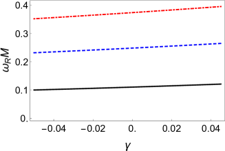
(a)  The real parts of the QNFs.

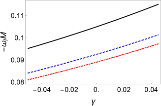
(b)  The imaginary parts of the QNFs.

Figure 2: The effect of the Lorentz-violating parameter $\gamma$ on the QNFs. The black, blue dashed, and red dot dashed lines denote the QNFs of the scalar field, electromagnetic field, and gravitational field, respectively.

The QNMs can tell us how the perturbations decay, but we do not know the amplitude of the perturbations. In order to understand the system more completely, we should investigate the time evolution of the the perturbed fields. In the time domain, we will use the null coordinates $u=t-r_{*}$ and $v=t+r_{*}$ to study the time evolution. The perturbation equation in the null coordinates can be rewritten as

$$4\frac{\partial^{2}\Psi^{s}}{\partial_{u}\partial_{v}}+V^{s}_{eff}\Psi^{s}=0.$$ (15)

The initial data is chosen to be a Gaussian wave packet in the $v$ coordinate

$$\Psi^{s}(0,v) = \exp(-\frac{(v-v_{c})^{2}}{2\sigma^{2}}),$$

$$\Psi^{s}(u,0) = 0.$$ (16)

The Gaussian wave packet is located at $v_{c}=10M$, and its width is $\sigma=1M$. The ranges of the $u,v$ coordinates are both $(0,500M)$. We extract the data at $r_{*}=50M$. The results of the time evolution for the three perturbed fields are shown in Fig. 3. From these figures, we can see that, the amplitude of the black lines ($\gamma=-0.05$) larger than that of the blue lines ($\gamma=0$) and the red lines ($\gamma=0.05$) in the QNMs dominate part. That is, the perturbed fields will decay more quickly as the Lorentz-violating parameter $\gamma$ increase. This is consistent with the result obtained in frequency domain. Besides, we can obtain the QNFs by fitting the data. The results agree well with that of frequency domain. For example, the fitted QNF for the black line of Fig. 3(c) (the gravitational field with $\gamma=-0.05$ and $k=2$) is $0.352431-0.082783i$. The result obtained by the continued fraction method is $0.351650-0.081002i$. Considering the numerical error, the two results agree well with each other.

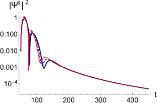
(a)

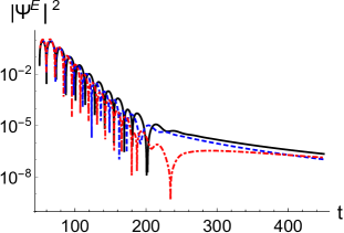
(b)

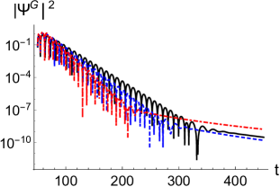
(c)

Figure 3: The time evolution for different perturbed fields. The mass $M$ is set to $M=1$, and the Lorentz violating parameter $\gamma$ is set to $\gamma=-0.05$ (the black lines), $\gamma=0$ (the blue dots), and $\gamma=0.05$ (the red dashed dots). (a) The time evolution for the scalar field and $l=0$. (b) The time evolution for the Maxwell field and $l=1$. (c) The time evolution for the gravitational field and $l=2$.

IV Greybody factor

Another very important aspect of perturbations around a black hole is the absorption cross-section. The greybody factor is defined as the probability of an outgoing wave reach to infinity or an incoming wave to be absorbed by the black hole Konoplya:2019ppy ; Cardoso:2005vb ; Dey:2018cws . Recently, it has been noted that the ringdown signal following an extreme mass ratio merger can be modelled using the greybody factor Oshita:2023cjz . So, it is very important to study the greybody factor of the Lorentz-violating black hole.

We will calculate the greybody factor through the WKB method Konoplya:2019hlu . The boundary condition for the scattering process is different from that of the QNMs, which can be written as

$$\Psi^{s} = e^{-i\omega r_{*}}+Re^{i\omega r_{*}},~{}~{}~{}~{}r_{*}\rightarrow+\infty,$$

$$\Psi^{s} = Te^{-i\omega r_{*}},~{}~{}~{}~{}~{}~{}~{}~{}~{}~{}~{}~{}~{}~{}r_{*}\rightarrow-\infty,$$ (17)

where $R$ and $T$ represent the reflection coefficient and transmission coefficient, respectively. From the boundary condition (17) we can see that, there are both ingoing wave and outgoing wave at infinity, but only ingoing wave at horizon. Using the 6th order WKB method, the reflection and transmission coefficients can be obtained

$$|R|^{2} = \frac{1}{1+e^{-2\pi iK}},$$ (18)

$$|T|^{2} = \frac{1}{1+e^{2\pi iK}}=1-|R|^{2},$$ (19)

where $K$ is a parameter which can be obtained by the WKB formula

$$K=\frac{i(\omega^{2}-V_{0})}{\sqrt{-2V_{0}^{\prime\prime}}}-\sum_{j=2}^{6}\Lambda_{j},$$ (20)

where the correction terms $\Lambda_{j}$ are the same as in Eq. (14) and are all imaginary numbers.

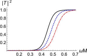
(a)  The greybody factor for the scalar field.

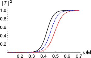
(b)  The greybody factor for the electromagnetic field.

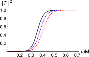
(c)  The greybody factor for the gravitational field.

Figure 4: The effect of the Lorentz-violating parameter $\gamma$ on the greybody factor for three perturbed fields. The black lines denote the greybody factor with $\gamma=-0.05$, the blue dashed lines denote the greybody factor with $\gamma=0$, and the red dot dashed lines denote the greybody factor with $\gamma=0.05$.

The greybody factor for the three perturbed fields are plotted in Fig. 4. From this figure we can see that, the greybody factor decrease with the parameter $\gamma$, which means that with the increasing of $\gamma$, a smaller fraction of the perturbed field can penetrate the potential barrier. This is consistent with the effective potential, where the height of the potential barrier increase with the parameter $\gamma$, which can be seen from Fig. 1.

V Conclusions

In this paper we studied the QNMs and the greybody factor in the background of a spherically symmetric Lorentz-violating black hole. The Lorentz symmetry is spontaneously broken due to the vacuum condensate of the KR field. The Lorentz-violating effect is represented by a parameter $\gamma$, which is named as the Lorentz-violating parameter.

We investigated three kinds of perturbed fields, the scalar field, odd parity electromagnetic field, and odd parity gravitational field. The perturbation equations for the odd parity perturbations can be written into a Schrödinger equation (4). The effective potentials were plotted in Fig. 1, from which we can see that the height of the effective potential barrier increases with the Lorentz-violating parameter $\gamma$. After choosing the boundary condition, the QNMs become a eigenvalue problem. We used three methods to solve the QNFs, i.e. the continued fraction method, direct integration method, and WKB method. The results are shown in Tables 1, 2, and 3. The QNFs obtained from the three methods agree well with each other, which confirms our results are correct. The effect of the Lorentz-violating parameter $\gamma$ on the QNFs is shown in Fig. 2. From this figure we showed that both the real parts and the absolute value of the imaginary parts of the QNFs increase with $\gamma$. For completeness, we studied the time evolution of the perturbed fields starting with a Gaussian wave packet. The results are shown in Fig. 3. From the numerical data, we fitted the QNFs, the results agree well with that of the frequency domain. Figure 3 shows that the perturbed fields will decay more quickly as the Lorentz-violating parameter $\gamma$ increase.

Using the 6th order WKB method, we also calculated the greybody factor for these three perturbed fields. The results are shown in Fig. 4. The effect of the Lorentz-violating parameter $\gamma$ shows that, the greybody factor decrease with the parameter $\gamma$. This is consistent with the effective potential.

VI Acknowledgments

We thank Ke Yang for very useful discussion on the Lorentz-violating black hole. This work was supported by National Key Research and Development Program of China (Grant No. 2020YFC2201503), the National Natural Science Foundation of China (Grants No. 12205129, No. 12147166, No. 11875151, and No. 12247101, No. 12347111), the China Postdoctoral Science Foundation (Grant No. 2021M701529 and No. 2023M741148), the 111 Project (Grant No. B20063), the Department of education of Gansu Province: Outstanding Graduate “Innovation Star” Project (Grant No. 2023CXZX-057), the Major Science and Technology Projects of Gansu Province, and Lanzhou City’s scientific research funding subsidy to Lanzhou University.

References

- (1) T. Jacobson and D. Mattingly, Gravity with a dynamical preferred frame, Phys. Rev. D 64 (2001), 024028 doi:10.1103/PhysRevD.64.024028 [arXiv:gr-qc/0007031 [gr-qc]].
- (2) P. Horava, Quantum Gravity at a Lifshitz Point, Phys. Rev. D 79 (2009), 084008 doi:10.1103/PhysRevD.79.084008 [arXiv:0901.3775 [hep-th]].
- (3) G. R. Bengochea and R. Ferraro, Dark torsion as the cosmic speed-up, Phys. Rev. D 79 (2009), 124019 doi:10.1103/PhysRevD.79.124019 [arXiv:0812.1205 [astro-ph]].
- (4) V. A. Kostelecky and S. Samuel, Spontaneous Breaking of Lorentz Symmetry in String Theory, Phys. Rev. D 39 (1989), 683 doi:10.1103/PhysRevD.39.683.
- (5) J. Alfaro, H. A. Morales-Tecotl, and L. F. Urrutia, Loop quantum gravity and light propagation, Phys. Rev. D 65 (2002), 103509 doi:10.1103/PhysRevD.65.103509 [arXiv:hep-th/0108061 [hep-th]].
- (6) V. A. Kostelecky, Gravity, Lorentz violation, and the standard model, Phys. Rev. D 69 (2004), 105009 doi:10.1103/PhysRevD.69.105009 [arXiv:hep-th/0312310 [hep-th]].
- (7) V. A. Kostelecky and S. Samuel, Gravitational Phenomenology in Higher Dimensional Theories and Strings, Phys. Rev. D 40 (1989), 1886-1903 doi:10.1103/PhysRevD.40.1886.
- (8) V. A. Kostelecky and S. Samuel, Phenomenological Gravitational Constraints on Strings and Higher Dimensional Theories, Phys. Rev. Lett. 63 (1989), 224 doi:10.1103/PhysRevLett.63.224.
- (9) Q. G. Bailey and V. A. Kostelecky, Signals for Lorentz violation in post-Newtonian gravity, Phys. Rev. D 74 (2006), 045001 doi:10.1103/PhysRevD.74.045001 [arXiv:gr-qc/0603030 [gr-qc]].
- (10) R. Bluhm, N. L. Gagne, R. Potting, and A. Vrublevskis, Constraints and Stability in Vector Theories with Spontaneous Lorentz Violation, Phys. Rev. D 77 (2008), 125007 [erratum: Phys. Rev. D 79 (2009), 029902] doi:10.1103/PhysRevD.79.029902 [arXiv:0802.4071 [hep-th]].
- (11) R. Casana, A. Cavalcante, F. P. Poulis, and E. B. Santos, Exact Schwarzschild-like solution in a bumblebee gravity model, Phys. Rev. D 97 (2018) no.10, 104001 doi:10.1103/PhysRevD.97.104001 [arXiv:1711.02273 [gr-qc]].
- (12) R. V. Maluf and J. C. S. Neves, Black holes with a cosmological constant in bumblebee gravity, Phys. Rev. D 103 (2021) no.4, 044002 doi:10.1103/PhysRevD.103.044002 [arXiv:2011.12841 [gr-qc]].
- (13) R. Xu, D. Liang, and L. Shao, Static spherical vacuum solutions in the bumblebee gravity model, Phys. Rev. D 107 (2023) no.2, 024011 doi:10.1103/PhysRevD.107.024011 [arXiv:2209.02209 [gr-qc]].
- (14) C. Ding, C. Liu, R. Casana, and A. Cavalcante, Exact Kerr-like solution and its shadow in a gravity model with spontaneous Lorentz symmetry breaking, Eur. Phys. J. C 80 (2020) no.3, 178 doi:10.1140/epjc/s10052-020-7743-y [arXiv:1910.02674 [gr-qc]].
- (15) C. Ding and X. Chen, Slowly rotating Einstein-bumblebee black hole solution and its greybody factor in a Lorentz violation model, Chin. Phys. C 45 (2021) no.2, 025106 doi:10.1088/1674-1137/abce51 [arXiv:2008.10474 [gr-qc]].
- (16) İ. Güllü and A. Övgün, Schwarzschild-like black hole with a topological defect in bumblebee gravity, Annals Phys. 436 (2022), 168721 doi:10.1016/j.aop.2021.168721 [arXiv:2012.02611 [gr-qc]].
- (17) C. Ding, X. Chen, and X. Fu, Einstein-Gauss-Bonnet gravity coupled to bumblebee field in four dimensional spacetime, Nucl. Phys. B 975 (2022), 115688 doi:10.1016/j.nuclphysb.2022.115688 [arXiv:2102.13335 [gr-qc]].
- (18) S. K. Jha and A. Rahaman, Bumblebee gravity with a Kerr-Sen-like solution and its Shadow, Eur. Phys. J. C 81 (2021) no.4, 345 doi:10.1140/epjc/s10052-021-09132-6 [arXiv:2011.14916 [gr-qc]].
- (19) C. Ding, Y. Shi, J. Chen, Y. Zhou, and C. Liu, High dimensional AdS-like black hole and phase transition in Einstein-bumblebee gravity*, Chin. Phys. C 47 (2023) no.4, 045102 doi:10.1088/1674-1137/aca8f4 [arXiv:2201.06683 [gr-qc]].
- (20) Z. F. Mai, R. Xu, D. Liang, and L. Shao, Extended thermodynamics of the bumblebee black holes, Phys. Rev. D 108 (2023) no.2, 024004 doi:10.1103/PhysRevD.108.024004 [arXiv:2304.08030 [gr-qc]].
- (21) H. M. Wang and S. W. Wei, Shadow cast by Kerr-like black hole in the presence of plasma in Einstein-bumblebee gravity, Eur. Phys. J. Plus 137 (2022) no.5, 571 doi:10.1140/epjp/s13360-022-02785-6 [arXiv:2106.14602 [gr-qc]].
- (22) C. Chen, Q. Pan, and J. Jing, Quasinormal modes of a scalar perturbation around a rotating BTZ-like black hole in Einstein-bumblebee gravity, Phys. Lett. B 846 (2023), 138186 doi:10.1016/j.physletb.2023.138186 [arXiv:2302.05861 [gr-qc]].
- (23) X. Zhang, M. Wang, and J. Jing, Quasinormal modes and late time tails of perturbation fields on a Schwarzschild-like black hole with a global monopole in the Einstein-bumblebee theory, Sci. China Phys. Mech. Astron. 66 (2023) no.10, 100411 doi:10.1007/s11433-023-2153-6 [arXiv:2307.10856 [gr-qc]].
- (24) R. H. Lin, R. Jiang, and X. H. Zhai, Quasinormal modes of the spherical bumblebee black holes with a global monopole, Eur. Phys. J. C 83 (2023) no.8, 720 doi:10.1140/epjc/s10052-023-11899-9 [arXiv:2308.01575 [gr-qc]].
- (25) Z. Wang, S. Chen, and J. Jing, Constraint on parameters of a rotating black hole in Einstein-bumblebee theory by quasi-periodic oscillations, Eur. Phys. J. C 82 (2022) no.6, 528 doi:10.1140/epjc/s10052-022-10475-x [arXiv:2112.02895 [gr-qc]].
- (26) B. Altschul, Q. G. Bailey, and V. A. Kostelecky, Lorentz violation with an antisymmetric tensor, Phys. Rev. D 81 (2010), 065028 doi:10.1103/PhysRevD.81.065028 [arXiv:0912.4852 [gr-qc]].
- (27) M. Kalb and P. Ramond, Classical direct interstring action, Phys. Rev. D 9 (1974), 2273-2284 doi:10.1103/PhysRevD.9.2273.
- (28) L. A. Lessa, J. E. G. Silva, R. V. Maluf, and C. A. S. Almeida, Modified black hole solution with a background Kalb–Ramond field, Eur. Phys. J. C 80 (2020) no.4, 335 doi:10.1140/epjc/s10052-020-7902-1 [arXiv:1911.10296 [gr-qc]].
- (29) K. Yang, Y. Z. Chen, Z. Q. Duan, and J. Y. Zhao, Static and spherically symmetric black holes in gravity with a background Kalb-Ramond field, [arXiv:2308.06613 [gr-qc]].
- (30) A. A. A. Filho, J. A. A. S. Reis, and H. Hassanabadi, Exploring antisymmetric tensor effects on black hole shadows and quasinormal frequencies, [arXiv:2309.15778 [gr-qc]].
- (31) B. P. Abbott et al. [LIGO Scientific and Virgo], Observation of Gravitational Waves from a Binary Black Hole Merger, Phys. Rev. Lett. 116 (2016) no.6, 061102 doi:10.1103/PhysRevLett.116.061102 [arXiv:1602.03837 [gr-qc]].
- (32) K. Akiyama et al. [Event Horizon Telescope], First M87 Event Horizon Telescope Results. I. The Shadow of the Supermassive Black Hole, Astrophys. J. Lett. 875 (2019), L1 doi:10.3847/2041-8213/ab0ec7 [arXiv:1906.11238 [astro-ph.GA]].
- (33) E. Berti, V. Cardoso, J. A. Gonzalez, and U. Sperhake, Mining information from binary black hole mergers: A Comparison of estimation methods for complex exponentials in noise, Phys. Rev. D 75 (2007), 124017 doi:10.1103/PhysRevD.75.124017 [arXiv:gr-qc/0701086 [gr-qc]].
- (34) H. P. Nollert and R. H. Price, Quantifying excitations of quasinormal mode systems, J. Math. Phys. 40 (1999), 980-1010 doi:10.1063/1.532698 [arXiv:gr-qc/9810074 [gr-qc]].
- (35) F. Echeverria, Gravitational Wave Measurements of the Mass and Angular Momentum of a Black Hole, Phys. Rev. D 40 (1989), 3194-3203 doi:10.1103/PhysRevD.40.3194.
- (36) E. Berti, V. Cardoso, and C. M. Will, On gravitational-wave spectroscopy of massive black holes with the space interferometer LISA, Phys. Rev. D 73 (2006), 064030 doi:10.1103/PhysRevD.73.064030 [arXiv:gr-qc/0512160 [gr-qc]].
- (37) E. Berti, J. Cardoso, V. Cardoso, and M. Cavaglia, Matched-filtering and parameter estimation of ringdown waveforms, Phys. Rev. D 76 (2007), 104044 doi:10.1103/PhysRevD.76.104044 [arXiv:0707.1202 [gr-qc]].
- (38) M. Isi, M. Giesler, W. M. Farr, M. A. Scheel, and S. A. Teukolsky, Testing the no-hair theorem with GW150914, Phys. Rev. Lett. 123 (2019) no.11, 111102 doi:10.1103/PhysRevLett.123.111102 [arXiv:1905.00869 [gr-qc]].
- (39) V. Cardoso, E. Franzin, and P. Pani, Is the gravitational-wave ringdown a probe of the event horizon?, Phys. Rev. Lett. 116 (2016) no.17, 171101 [erratum: Phys. Rev. Lett. 117 (2016) no.8, 089902] doi:10.1103/PhysRevLett.116.171101 [arXiv:1602.07309 [gr-qc]].
- (40) V. Cardoso and P. Pani, Testing the nature of dark compact objects: a status report, Living Rev. Rel. 22 (2019) no.1, 4 doi:10.1007/s41114-019-0020-4 [arXiv:1904.05363 [gr-qc]].
- (41) V. Cardoso and P. Pani, Tests for the existence of black holes through gravitational wave echoes, Nature Astron. 1 (2017) no.9, 586-591 doi:10.1038/s41550-017-0225-y [arXiv:1709.01525 [gr-qc]].
- (42) J. L. Jaramillo, R. Panosso Macedo, and L. Al Sheikh, Pseudospectrum and Black Hole Quasinormal Mode Instability, Phys. Rev. X 11 (2021) no.3, 031003 doi:10.1103/PhysRevX.11.031003 [arXiv:2004.06434 [gr-qc]].
- (43) M. H. Y. Cheung, K. Destounis, R. P. Macedo, E. Berti, and V. Cardoso, Destabilizing the Fundamental Mode of Black Holes: The Elephant and the Flea, Phys. Rev. Lett. 128 (2022) no.11, 111103 doi:10.1103/PhysRevLett.128.111103 [arXiv:2111.05415 [gr-qc]].
- (44) E. Berti, V. Cardoso, M. H. Y. Cheung, F. Di Filippo, F. Duque, P. Martens, and S. Mukohyama, Stability of the fundamental quasinormal mode in time-domain observations against small perturbations, Phys. Rev. D 106 (2022) no.8, 084011 doi:10.1103/PhysRevD.106.084011 [arXiv:2205.08547 [gr-qc]].
- (45) T. Torres, From Black Hole Spectral Instability to Stable Observables, Phys. Rev. Lett. 131 (2023) no.11, 111401 doi:10.1103/PhysRevLett.131.111401 [arXiv:2304.10252 [gr-qc]].
- (46) G. Guo, P. Wang, H. Wu, and H. Yang, Quasinormal modes of black holes with multiple photon spheres, JHEP 06 (2022), 060 doi:10.1007/JHEP06(2022)060 [arXiv:2112.14133 [gr-qc]].
- (47) V. Cardoso, W. D. Guo, C. F. B. Macedo, and P. Pani, The tune of the Universe: the role of plasma in tests of strong-field gravity, Mon. Not. Roy. Astron. Soc. 503 (2021) no.1, 563-573 doi:10.1093/mnras/stab404 [arXiv:2009.07287 [gr-qc]].
- (48) W. D. Guo, Q. Tan, and Y. X. Liu, Gravitoelectromagnetic coupled perturbations and quasinormal modes of a charged black hole with scalar hair, Phys. Rev. D 107 (2023) no.12, 124046 doi:10.1103/PhysRevD.107.124046 [arXiv:2212.08784 [gr-qc]].
- (49) S. Yang, W. D. Guo, Q. Tan, and Y. X. Liu, Axial gravitational quasinormal modes of a self-dual black hole in loop quantum gravity, Phys. Rev. D 108 (2023) no.2, 024055 doi:10.1103/PhysRevD.108.024055 [arXiv:2304.06895 [gr-qc]].
- (50) W. D. Guo and Q. Tan, Quasinormal Modes of a Charged Black Hole with Scalar Hair, Universe 9 (2023) no.7, 320 doi:10.3390/universe9070320.
- (51) H. H. Li, S. J. Yang, and S. W. Wei, The fastest relaxation rate of Born-Infeld black hole, Gen. Rel. Grav. 54 (2022) no.1, 1 doi:10.1007/s10714-021-02888-y.
- (52) S. S. Seahra, Ringing the Randall-Sundrum braneworld:Metastable gravity wave bound states, Phys. Rev. D 72 (2005), 066002 doi:10.1103/PhysRevD.72.066002 [arXiv:hep-th/0501175 [hep-th]].
- (53) Q. Tan, W. D. Guo, and Y. X. Liu, Sound from extra dimensions: Quasinormal modes of a thick brane, Phys. Rev. D 106 (2022) no.4, 044038 doi:10.1103/PhysRevD.106.044038 [arXiv:2205.05255 [gr-qc]].
- (54) R. A. Konoplya and A. F. Zinhailo, Hawking radiation of non-Schwarzschild black holes in higher derivative gravity: a crucial role of grey-body factors, Phys. Rev. D 99 (2019) no.10, 104060 doi:10.1103/PhysRevD.99.104060 [arXiv:1904.05341 [gr-qc]].
- (55) V. Cardoso, M. Cavaglia, and L. Gualtieri, Black Hole Particle Emission in Higher-Dimensional Spacetimes, Phys. Rev. Lett. 96 (2006), 071301 [erratum: Phys. Rev. Lett. 96 (2006), 219902] doi:10.1103/PhysRevLett.96.071301 [arXiv:hep-th/0512002 [hep-th]].
- (56) S. Dey and S. Chakrabarti, A note on electromagnetic and gravitational perturbations of the Bardeen de Sitter black hole: quasinormal modes and greybody factors, Eur. Phys. J. C 79 (2019) no.6, 504 doi:10.1140/epjc/s10052-019-7004-0 [arXiv:1807.09065 [gr-qc]].
- (57) P. Kanti and J. March-Russell, Calculable corrections to brane black hole decay. 1. The scalar case, Phys. Rev. D 66 (2002), 024023 doi:10.1103/PhysRevD.66.024023 [arXiv:hep-ph/0203223 [hep-ph]].
- (58) S. W. Hawking, Particle Creation by Black Holes, Commun. Math. Phys. 43 (1975), 199-220 [erratum: Commun. Math. Phys. 46 (1976), 206] doi:10.1007/BF02345020.
- (59) N. Oshita, Greybody Factors Imprinted on Black Hole Ringdowns: an alternative to superposed quasi-normal modes, [arXiv:2309.05725 [gr-qc]].
- (60) R. Bluhm, S. H. Fung, and V. A. Kostelecky, Spontaneous Lorentz and Diffeomorphism Violation, Massive Modes, and Gravity, Phys. Rev. D 77 (2008), 065020 doi:10.1103/PhysRevD.77.065020 [arXiv:0712.4119 [hep-th]].
- (61) A. R. Ruffini, Angular momentum in quantum mechanics, (Princeton University Press, Princeton, 1996).
- (62) T. Regge and J. A. Wheeler, Stability of a Schwarzschild Singularity, Phys. Rev. 108, (1957) 1063.
- (63) E. W. Leaver, An analytic representation for the quasi-normal modes of Kerr black holes, Proc. R. Soc. Lond. A 402, 285-298 (1985).
- (64) P. Pani, Advanced Methods in Black-Hole Perturbation Theory, Int. J. Mod. Phys. A 28 (2013), 1340018 doi:10.1142/S0217751X13400186 [arXiv:1305.6759 [gr-qc]].
- (65) R. A. Konoplya, Quasinormal behavior of the d-dimensional Schwarzschild black hole and higher order WKB approach, Phys. Rev. D 68 (2003), 024018 doi:10.1103/PhysRevD.68.024018 [arXiv:gr-qc/0303052 [gr-qc]].
- (66) S. Iyer and C. M. Will, Black Hole Normal Modes: A WKB Approach. 1. Foundations and Application of a Higher Order WKB Analysis of Potential Barrier Scattering,S Phys. Rev. D 35 (1987), 3621 doi:10.1103/PhysRevD.35.3621.
- (67) R. A. Konoplya, On quasinormal modes of small Schwarzschild-anti-de Sitter black hole, Phys. Rev. D 66 (2002), 044009 doi:10.1103/PhysRevD.66.044009 [arXiv:hep-th/0205142 [hep-th]].
- (68) R. A. Konoplya, A. Zhidenko, and A. F. Zinhailo, Higher order WKB formula for quasinormal modes and grey-body factors: recipes for quick and accurate calculations, Class. Quant. Grav. 36 (2019), 155002 doi:10.1088/1361-6382/ab2e25 [arXiv:1904.10333 [gr-qc]].