scRNA-seq Data Clustering by Cluster-aware Iterative Contrastive Learning

Abstract

Single-cell RNA sequencing (scRNA-seq) enables researchers to analyze gene expression at single-cell level. One important task in scRNA-seq data analysis is unsupervised clustering, which helps identify distinct cell types, laying down the foundation for other downstream analysis tasks. In this paper, we propose a novel method called Cluster-aware Iterative Contrastive Learning (CICL in short) for scRNA-seq data clustering, which utilizes an iterative representation learning and clustering framework to progressively learn the clustering structure of scRNA-seq data with a cluster-aware contrastive loss. CICL consists of a Transformer encoder, a clustering head, a projection head and a contrastive loss module. First, CICL extracts the feature vectors of the original and augmented data by the Transformer-encoder. Then, it computes the clustering centroids by K-means and employs the student’s t-distribution to assign pseudo-labels to all cells in the clustering head. The projection-head uses a Multi-Layer Perceptron (MLP) to obtain projections of the augmented data. At last, both pseudo-labels and projections are used in the contrastive loss to guide the model training. Such a process goes iteratively so that the clustering result becomes better and better. Extensive experiments on 25 real-world scRNA-seq datasets show that CICL outperforms the state-of-the-art (SOTA) methods. Concretely, CICL surpasses the existing methods by from 14% to 280%, and from 5% to 133% on average in terms of performance metrics ARI and NMI respectively. Source code is available at https://github.com/Alunethy/CICL.

1 Introduction

Each cell possesses unique characteristics and biological functions defined by its gene transcription activities. Conventional bulk RNA sequencing measures the average transcription levels of a multitude of cells, thereby obscuring the heterogeneity among individual cells. In the past decade, the rapid progress of single-cell RNA sequencing (scRNA-seq) technologies (Tang et al., 2009) enables transcriptome-wide gene expression measurement in individual cells, which greatly helps deepen our understanding of cellular heterogeneity and propels the research on cell biology, immunology, and complex diseases (van Galen et al., 2019). Identifying cell types is a fundamental step in unraveling complex biological processes such as cellular differentiation, lineage commitment, and gene regulation (Deng et al., 2021). As such, cell clustering becomes an important task in scRNA-seq analysis. However, the inherent high-dimensionality, noise, and sparsity of scRNA-seq data present severe challenges for scRNA-seq data clustering analysis (Kiselev et al., 2019; Stegle et al., 2015).

Up to now, many models or algorithms have been developed for scRNA-seq data clustering. Early scRNA-seq clustering methods mainly rely on traditional dimensionality reduction and clustering methods. For example, pcaReduce (Žurauskienė and Yau, 2016) combines PCA and K-means, iteratively merging cluster pairs based on related probability density function. Recognizing the importance of similarity metrics in the clustering task, SIMLR (Wang et al., 2018a) amalgamates multiple kernels to learn sample similarity and perform spectral clustering. Seurat (Satija et al., 2015) employs a graph-based community detection algorithm, while Louvain (Blondel et al., 2008) is based on the shared nearest neighbor graph to identify cell types.

In the past decade, with the rapid development of deep learning, deep neural networks (DNN) have been extensively applied to scRNA-seq data clustering to address the limitations of conventional methods (Flores et al., 2022). DEC (Xie et al., 2016) and IDEC (Guo et al., 2017), based on autoencoders (AE), use KL divergence as the clustering loss, achieving simultaneous learning of feature representations and cluster assignments. To address the pervasive dropout events in scRNA-seq data, DCA (Eraslan et al., 2019) proposes a zero-inflated negative binomial (ZINB) model to better characterize the distribution of scRNA-seq data, and uses the negative likelihood as the reconstruction loss instead of the frequently-used mean-square error (MSE) loss in autoencoders. scVI (Lopez et al., 2018) is a deep generative model based on variational autoencoders, which can do various scRNA-seq data analyses such as data imputation, clustering, and visualization. scDeepCluster (Tian et al., 2019) introduces a novel model-based deep learning clustering approach. By combining the ZINB model with the DEC algorithm, it is designed to capture the underlying cluster structure of scRNA-seq data. scDHA (Tran et al., 2021) exploits a stacked Bayesian self-learning network to learn compact and generalized representations of scRNA-seq data.

Fig. 1: The framework of CICL. We first generate two augmented views $X_{aug1}$ and $X_{aug2}$ of the raw data $X$ by adding Gaussian noise. Then, we obtain the representations $H$, $H_{aug1}$ and $H_{aug2}$ of $X$, $X_{aug1}$ and $X_{aug2}$ by a transformer encoder. Next, we perform K-means on $H$ to get the centroid matrix $C$. After that, we feed $H$ and $C$ to the clustering-head and get a pseudo-label for each cell. Meanwhile, the projection-head encodes the $H_{aug1}$ and $H_{aug2}$ to obtain their projections $Z_{aug1}$ and $Z_{aug2}$. Finally, by using a novel contrastive loss, we align the positive pairs and contrast the negative pairs simultaneously. This process forms a loop to improve representations and clustering iteratively.

To leverage the relationships between cells, some studies construct the cell-cell graph and apply Graph Neural Networks (GNNs) to learn the representations of cells. scDSC (Gan et al., 2022) formulates and aggregates cell-cell relationships with graph neural networks and learns latent gene expression patterns using a ZINB model based autoencoder. GraphSCC (Zeng et al., 2020) integrates the structural relationships between cells into scRNA-seq clustering by employing a graph convolutional network. It also utilizes a dual self-supervised module to cluster cells and guide the training process. Furthermore, Some other works have tried to train models using manual annotations as supervisory information or prior knowledge, as demonstrated in transfer learning and meta-learning methods (Hu et al., 2020). While these methods can deliver excellent results on specific datasets, they also face serious challenge of scalability.

Contrastive learning (CL) has been widely used in computer vision and natural language processing (Chen et al., 2020; He et al., 2020). There have also been endeavors to incorporate contrastive learning into scRNA-seq data clustering. For instance, contrastive-sc (Ciortan and Defrance, 2021) proposes a contrastive learning based method for scRNA-seq data by masking a certain proportion of data features to obtain augmented data. Similar to most practices in contrastive learning, this method designates augmented pairs as positive samples, while considering all other pairs as negatives. scNAME (Wan et al., 2022) improves the conventional contrastive loss by proposing a new neighborhood contrastive loss combined with an ancillary mask estimation task, characterizing feature correlation and pairwise cell similarity better. CLEAR (Han et al., 2022) employs multiple data augmentation methods to simulate different noise types, uses the infoNCE (Oord et al., 2018) loss as a contrastive loss, and generates feature representations for scRNA-seq data with the momentum update strategy of encoder. However, these methods mainly apply the standard contrastive learning directly, failing to adapt the selection of positive and negative samples to the clustering task.

This paper aims to boost the performance of scRNA-seq data clustering by exploring new methods. Our contributions are two-fold. On the one hand, we propose a Cluster-aware Iterative Contrastive Learning (CICL) method for scRNA-seq data clustering. CICL employs an iterative representation learning and clustering framework with a cluster-aware contrastive loss, it can progressively improve the clustering result by comprehensively exploiting the hidden cluster structure for scRNA-seq data representation. On the other hand, we conduct extensive experiments on 25 real-world datasets, which show that our method outperforms the SOTA methods in most cases.

2 Materials and Methods

2.1 Datasets and Performance Metrics

The proposed CICL method is evaluated on 25 real scRNA-seq datasets, and each dataset contains cells whose labels are known as prior or validated in the previous studies. The 25 datasets were derived from 7 different sequencing platforms. The smallest dataset contains only 90 cells, while the largest dataset has 48,266 cells. The number of cell subtypes in these datasets ranges from 2 to 15. Statistics of these datasets are presented in Table 1.

Table 1: Datasets used in our experiments.

Dataset	Platform	#Cells	#Genes	#Subtypes
Adam (Adam et al., 2017)	Drop-seq	3660	23797	8
Bach (Bach et al., 2017)	10X	23184	19965	8
Bladder (Consortium, 2020)	10X	2432	22966	2
deng (Deng et al., 2014)	Smart-seq2	268	22431	6
Diaphragm (Consortium, 2020)	10X	1858	22966	6
hrvatin (Hrvatin et al., 2018)	Drop-seq	48266	25187	8
Klein (Klein et al., 2015)	inDrop	2717	24047	4
kolodziejczyk (Kolodziejczyk et al., 2015)	SMARTer	704	38616	3
Limb_Muscle (Consortium, 2020)	10X	3855	22966	6
Mammary_Gland (Consortium, 2020)	10X	3282	22966	4
muraro (Muraro et al., 2016)	CEL-seq2	2126	19127	10
Plasschaert (Plasschaert et al., 2018)	inDrop	6977	28205	8
pollen (Pollen et al., 2014)	SMARTer	301	23730	11
Qx_Spleen (Schaum et al., 2018)	10X	9552	23341	5
Qx_Trachea (Schaum et al., 2018)	10X	11269	23341	5
QS_Diaphragm (Schaum et al., 2018)	Smart-seq2	870	23341	5
QS_Heart (Schaum et al., 2018)	Smart-seq2	4365	23341	8
QS_Limb_Muscle (Schaum et al., 2018)	Smart-seq2	1090	23341	6
QS_Lung (Schaum et al., 2018)	Smart-seq2	1676	23341	11
QS_Trachea (Schaum et al., 2018)	Smart-seq2	1350	23341	4
Romanov (Romanov et al., 2017)	SMARTer	2881	21143	7
Tosches_turtle (Tosches et al., 2018)	Drop-seq	18664	23500	15
Wang_lung (Wang et al., 2018b)	10X	9519	14561	2
yan (Yan et al., 2013)	Tang	90	20214	6
Young (Young et al., 2018)	10X	5685	33658	11

We preprocess the scRNA-seq data with the Python package SCANPY (Wolf et al., 2018), following the strategy in (Tian et al., 2019). Specifically, given the raw read counts (i.e., gene expression matrix), we first filter out cells and genes without counts. Then, we calculate the library size of each cell as the total number of read counts per cell, and obtain the size factor of each cell via dividing its library size by the median of all library sizes. Thirdly, we obtain the normalized read count by dividing the raw read count with the size factor of each cell, followed by a natural $log$ transformation. Furthermore, we consider only the top-$t$ highly variable genes according to their normalized dispersion values, and set $t$ to 500 by default in our paper. Finally, we transform the normalized read counts into z-score data.

Two widely used metrics, normalized mutual information (NMI) and adjusted rand index (ARI) are used to evaluate clustering performance. NMI measures the similarity between the predicted labels and the real labels. Specifically, given the predicted labels $U=\left[u_{1},u_{2},...,u_{N}\right]\in\mathbb{R}^{N}$ and the real labels $V=\left[v_{1},v_{2},...,v_{N}\right]\in\mathbb{R}^{N}$, $N$ denotes the number of cells, NMI is evaluated as follows:

$$NMI=\frac{I(U,V)}{max(H(U),H(V))}$$ (1)

where $I(U,V)=\sum_{u}\sum_{v}p(u,v)log\frac{p(u,v)}{p(u)p(v)}$ calculates the mutual information between $U$ and $V$, $p(u,v)$ is the joint distribution of $U$ and $V$, $p(u)$ and $p(v)$ are marginal distributions respectively. $H(U)=\sum_{u}p(u)log(p(u))$ is the entropy of clustering $U$. Similarly, $H(V)=\sum_{v}p(v)log(p(v))$.

ARI was also used to measure the similarity between clustering results and true categories. It solves the problem of insufficient punishment of RI and considers the impact of random assignments. The value of ARI ranges from -1 to 1. The larger the value, the more similar the clustering result is to the real categories. ARI is defined as

$$ARI=\frac{\begin{matrix}\sum_{ij}{n_{ij}\choose 2}\end{matrix}-[\begin{matrix}\sum_{i}{a_{i}\choose 2}\end{matrix}\begin{matrix}\sum_{j}{b_{j}\choose 2}\end{matrix}]/{N\choose 2}}{[\begin{matrix}\sum_{i}{a_{i}\choose 2}\end{matrix}\begin{matrix}\sum_{j}{b_{j}\choose 2}\end{matrix}]/2-[\begin{matrix}\sum_{i}{a_{i}\choose 2}\end{matrix}\begin{matrix}\sum_{j}{b_{j}\choose 2}\end{matrix}]/{N\choose 2}}$$ (2)

where $n_{ij}$ denotes the number of cells in both cluster $i$ of $U$ and cluster $j$ of $V$, and $a_{i}$ denotes the count of cells assigned to cluster $i$ of $U$, $b_{j}$ indicates the count of cells assigned to cluster $j$ of $V$.

2.2 The CICL Method

2.2.1 Overview

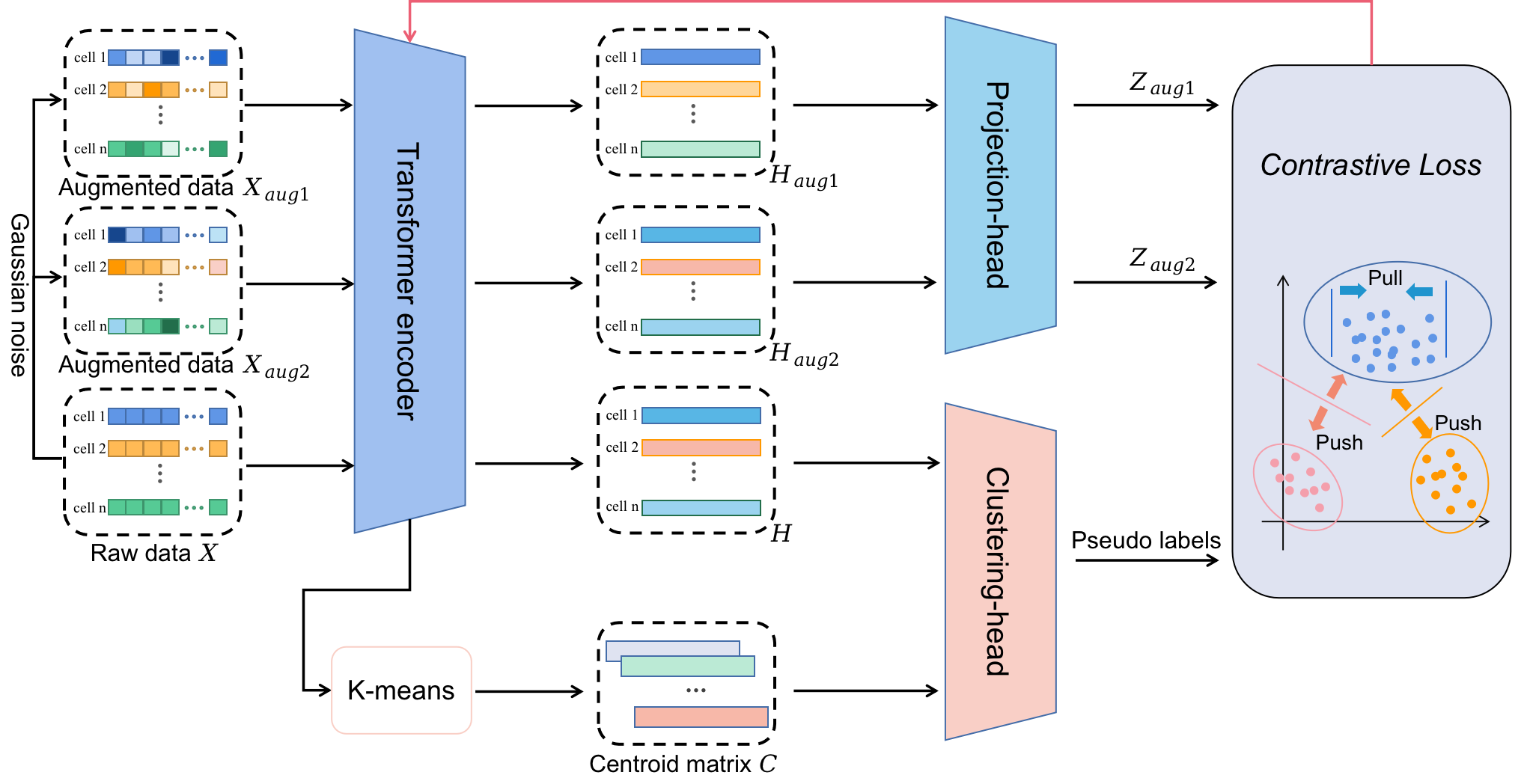
CICL is a cluster-aware iterative contrastive learning method designed for clustering scRNA-seq data, its framework is illustrated in Fig. 1. Specifically, in the model training phase, we first generate two augmented views $X_{aug1}$ and $X_{aug2}$ of the raw data $X$ by adding noise that is randomly sampled from Gaussian $N(0,1)$ and is mapped to the range [0, 1] via a linear transformation. Then, $X$, $X_{aug1}$ and $X_{aug2}$ are input into a transformer encoder (Vaswani et al., 2017) to obtain their representations $H$, $H_{aug1}$ and $H_{aug2}$, respectively. Next, we perform K-means on $H$ to get the centroid matrix $C=[c_{1},c_{2},...,c_{K}]$ where $c_{i}$ is the centroid vector of cluster $i$. The number of centroids is equal to the number of cell subtypes (or clusters) in the training dataset. After that, $H$ and $C$ are fed to the clustering-head and generate a pseudo-label for each cell. Meanwhile, the projection-head encodes $H_{aug1}$ and $H_{aug2}$ to obtain their projections $Z_{aug1}$ and $Z_{aug2}$. Finally, in addition to the traditional instance-wise contrastive loss, we propose a novel cluster-aware contrastive loss to align the positive pairs and contrast the negative pairs simultaneously, which takes the projections $Z_{aug1}$, $Z_{aug2}$ and pseudo-labels as input. We construct the positive pairs by an instance-wise way and a pseudo-label based way. In particular, an instance-wise positive pair consists of the representations of the two augmented copies of each cell, and a pseudo-label positive pair is formed by the representations of two augmented copies of two cells with similar pseudo-label (i.e., belonging to the same cluster). This training process goes iteratively. In the clustering phase, the input data $X$ are preprocessed and encoded by the trained transformer encoder to obtain the representation $H$. Then, $H$ are clustered by K-means to generate the final clustering result. In the following sections, we present the major components of our method in detail.

2.2.2 Transformer Encoder

The raw scRNA-seq data is modeled as a matrix $X\in\mathbb{R}^{N\times G}$ where $N$ indicates the number of cells and $G$ denotes the number of genes. To begin with, we construct augmented data by adding Gaussian noise, and two augmented copies (or views) $X_{aug1}$ and $X_{aug2}$ are generated for $X$. Then, we encode $X_{aug1}$, $X_{aug2}$ and $X$ by a transformer encoder, which has four layers, each of which consists of two networks: a multi-head self-attention network and a position-wise fully connected feed-forward network, each of them is followed by a residual connection and layer normalization. For example, give the input $X$ of the self-attention layer, the output is as follows:

$$H_{MulitHead}=Concat(Att_{1}(XW_{1}^{v}),...,Att_{h}(XW_{h}^{v}))W^{O}$$ (3)

where $W_{i}^{v}\in\mathbb{R}^{G\times d}$ and $W^{O}\in\mathbb{R}^{hd\times G}$ are learnable parameter matrices, $h$ is the number of heads. And $Att_{i}$ is evaluated by

$$Att_{i}=softmax(\frac{XW_{i}^{q}\times(XW_{i}^{k})^{\mathsf{T}}}{\sqrt{d}}),i=1,2,...,h$$ (4)

Above, $W_{i}^{q}\in\mathbb{R}^{G\times d}$ and $W_{i}^{k}\in\mathbb{R}^{G\times d}$ are learnable parameter matrices. Then, after the residual connection and layer normalization, we have

$$H_{res}=LayerNorm(X+H_{MulitHead})$$ (5)

The fully connected feed-forward network consists of two linear layers, following a rectified linear activation function (ReLU), so we have

$$H_{fc}=ReLU(H_{res}W_{1})W_{2}$$ (6)

where $W_{1}$ and $W_{2}$ are learnable parameter matrices. Finally, the output of the $i$-th layer of the transformer encoder is

$$H_{i}=LayerNorm(H_{fc}+H_{res})$$ (7)

2.2.3 Clustering-head and Pseudo-label Generation

Traditional contrastive loss suffers from sampling bias (Oord et al., 2018). For example, given a cell $i$, all the other cells are considered as its negative samples. However, these negative samples contain some cells of the same type as cell $i$, which will be undesirably pushed away from cell $i$ in the representation space by current contrastive learning.

To address this problem, CICL employs a cluster-aware contrastive learning strategy. To this end, we cluster the training data $H$ by K-means, and each cluster is characterized by its centroid $c_{i}$ in the representation space, which will be updated iteratively. Then, in the clustering-head, we use the Student’s t-distribution to compute the probability $q_{ij}$ that cell $i$ belongs to the $j$-th cluster,

$$q_{ij}=\frac{(1+\|h_{i}-c_{j})\|_{2}^{2}/\alpha)^{-\frac{\alpha+1}{2}}}{\sum_{k=1}^{K}(1+\|h_{i}-c_{k})\|_{2}^{2}/\alpha)^{-\frac{\alpha+1}{2}}}$$ (8)

where $h_{i}$ is the representation of cell $i$ in $H$. $\alpha$ is the degree of freedom of the Student’s t-distribution, we set $\alpha=1$ in this paper. Finally, we obtain the pseudo-label $l_{i}$ of cell $i$ by the probability vector $q_{i}$=$(q_{i1},q_{i2},...,q_{iK})$ as follows:

$$l_{i}=label\_assign(q_{i})$$ (9)

where $label\_assign$ is a function that returns the cluster index corresponding the maximum $q_{ij}$ ($j\in 1,2,...,K$). Thus, we obtain the pseudo-labels $L$=($l_{1}$, $l_{2}$, …, $l_{N}$) of all cells, which are used for contrastive loss computation. Note that each cell and its two augmented copies have the same pseudo-label. We use the term “pseudo-label” because they are just intermediate (not final) cluster labels.

2.2.4 Projection-head and Contrastive Learning Losses

We project $H_{aug1}$ and $H_{aug2}$ to obtain projections $Z_{aug1}$ and $Z_{aug2}$ by the projection-head, which is composed of a two-layer perceptron. Formally,

$$Z_{aug1}=W_{3}ReLU(W_{4}H_{aug1})$$ (10)

$$Z_{aug2}=W_{3}ReLU(W_{4}H_{aug2})$$ (11)

where $W_{3}$ and $W_{4}$ are learnable parameters. ReLU is the activation function. Let $z_{i}$ and $z^{{}^{\prime}}_{i}$ be the $i$-th row of $Z_{aug1}$ and $Z_{aug2}$ respectively, which correspond to the representations of cell $i$ in the two augmented views. For $z_{i}$, we not only treat $z_{i}$ and $z^{{}^{\prime}}_{i}$, but also $z_{i}$ and any other sample of the same cluster in terms of pseudo-label as a positive pair, while $z_{i}$ and any sample of the other clusters as a negative pair. Given the batch size $B$, we consider two losses as follows:

Instance-wise contrastive loss. CICL computes the infoNCE loss (Chen et al., 2020) for each cell. For cell $i$ with two views $z_{i}$ and $z_{i}^{{}^{\prime}}$, its contrastive loss in terms of $z_{i}$ is

where $\mathbb{I}_{i\neq m}$ is an indicator function whose value is 1 if $i\neq m$, otherwise is 0. $T$ is the temperature parameter set to 0.5 in our paper. The similarity function $sim(.,.)$ adopts point product or cosine similarity, i.e.,

$$sim{(z_{i},z_{i}^{{}^{\prime}})}=\frac{\|z_{i}^{T}z_{i}^{{}^{\prime}}\|}{\|z_{i}\|\|z_{i}^{{}^{\prime}}\|}$$ (13)

The overall instance-wise contrastive loss is

$$\mathcal{L}_{ins}=\frac{1}{2B}\sum^{B}_{i=1}[l_{ins}(z_{i})+l_{ins}(z^{{}^{\prime}}_{i})]$$ (14)

where $l_{ins}(z^{{}^{\prime}}_{i})$ is cell $i$’s contrastive loss in terms of $z^{{}^{\prime}}_{i}$. With this instance-wise contrastive loss, CICL can learn the representations well by pulling positive pairs together and pushing negative pairs away in the cell representation space.

Cluster-aware contrastive loss. To solve the sample bias, we propose a novel cluster-aware contrastive loss, which is evaluated with the pseudo-labels $L$, $Z_{aug1}$ and $Z_{aug2}$. We treat the pairs of representations of the same pseudo-label as positive pairs, and the remaining pairs as negative pairs. For cell $i$, its cluster-aware contrastive loss in terms of $z_{i}$ is as follows:

where $l_{i}$ is the pseudo-label of $z_{i}$. $E_{z_{i},z^{{}^{\prime}}_{j}\in l_{i}}$ is an indicator function whose value is 1 if the label of $z^{{}^{\prime}}_{j}$ is $l_{i}$, and 0 otherwise. $E_{z_{i},z^{{}^{\prime}}_{j}\notin l_{i}}$ is also an indicator function whose value is 0 if the label of $z^{{}^{\prime}}_{j}$ is $l_{i}$, and 1 otherwise. The overall cluster-aware loss is as follows:

$$\mathcal{L}_{clu}=\frac{1}{2B}\sum_{i=1}^{B}[l_{clu}(z_{i})+l_{clu}(z^{{}^{\prime}}_{i})]$$ (16)

where $l_{clu}(z^{{}^{\prime}}_{i})$ is cell $i$’s cluster-aware contrastive loss in terms of $z^{{}^{\prime}}_{i}$. This loss is particularly effective because it tries to minimize the distance between cells of similar cluster and maximize the distance between cells of different clusters.

Finally, by combining $\mathcal{L}_{ins}$ and $\mathcal{L}_{clu}$ with the hyperparameter $\lambda$, we have the whole loss function as follows:

$$\mathcal{L}=\mathcal{L}_{ins}+\lambda\mathcal{L}_{clu}$$ (17)

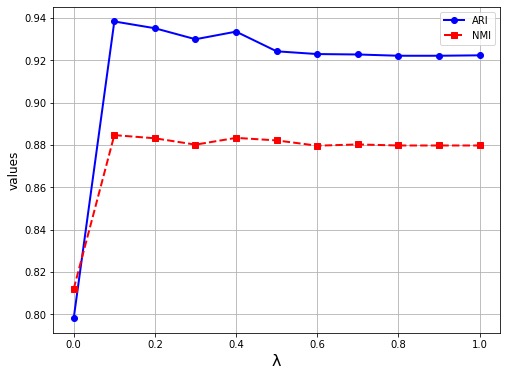
We set $\lambda=0.1$ in our experiments. A small $\lambda$ can prevent the negative effect of clustering error of K-means. With this loss, CICL exploits the cluster structure underlying the data to achieve simultaneous optimization of data representation and cluster label assignment. Compared with traditional contrastive learning, ours is iterative contrastive learning, which iteratively learns the representations of cells in the direction favorable for clustering.

2.3 Algorithm

Here, we present the algorithm of our method in Alg. 1, which consists of two phases: the training phase and the clustering phase. In the training phase, in each epoch we first randomly split the training data $X^{train}$ into $n_{B}$=$[X^{train}/S_{B}]$ minbatches. And for each minbatch $X^{j}$, we generate two augmented views $X^{j}_{aug1}$ and $X^{j}_{aug2}$. Next, we obtain the representations $H^{j}_{aug1}$, $H^{j}_{aug2}$ and $H^{j}$ of $X^{j}_{aug1}$, $X^{j}_{aug2}$ and $X^{j}$ by a transformer encoder. We perform K-means on $H^{j}$ to get centroid matrix $C^{j}$, and then the pseudo-labels $L^{j}$ are obtained from $H^{j}$ and $C^{j}$. Meanwhile, $H^{j}_{aug1}$, $H^{j}_{aug2}$ are input into the projection-head for obtaining projections $Z^{j}_{aug1}$ and $Z^{j}_{aug2}$. The whole loss $\mathcal{L}$ consists of $\mathcal{L}_{ins}$ and $\mathcal{L}_{clu}$, which are computed with $Z^{j}_{aug1}$, $Z^{j}_{aug2}$ and $L^{j}$ by Equ. (14) and Equ. (16) respectively. In the training phase, we use K-means to cluster the representations $H^{test}$ of testing data $X^{test}$, encoded by the trained transformer encoder, to generate the clustering result $R^{test}$.

Input : Training data $X^{train}$;

Testing data $X^{test}$;

The number of training epochs $n_{epoch}$;

Minibatch size $S_{B}$;

Output : Clustering result $R^{test}$ of $X^{test}$;

Training phase:

for $i$=1 to $n_{epoch}$ do

      $n_{B}$=$[X^{train}/S_{B}]$;

       Randomly split $X^{train}$ into $n_{B}$ minibatches;

       for each minibatch $X^{j}$ do

             Generate views $X^{j}_{aug1}$ and $X^{j}_{aug2}$ of $X^{j}$ by adding Gaussian noise;

             Obtain representations $H^{j}$, $H^{j}_{aug1}$, $H^{j}_{aug2}$ of $X^{j}$, $X^{j}_{aug1}$, $X^{j}_{aug2}$ by a transformer encoder;

             Generate centroid matrix $C^{j}$ of $H^{j}$ by K-means;

             Generate pseudo-labels $L^{j}$ with $H^{j}$ and $C^{j}$ by Equ. 8 and Equ. 9;

             Obtain projections $Z^{j}_{aug1}$ and $Z^{j}_{aug2}$ of $H^{j}_{aug1}$ and $H^{j}_{aug2}$ by the projection-head;

             Compute $\mathcal{L}_{ins}$ using $Z^{j}_{aug1}$ and $Z^{j}_{aug2}$ by Equ. 14;

             Compute $\mathcal{L}_{clu}$ using $Z^{j}_{aug1}$, $Z^{j}_{aug2}$ and $L$ by Equ. 16;

             Compute the whole loss $\mathcal{L}=\mathcal{L}_{ins}+\lambda\mathcal{L}_{clu}$ with $\lambda=0.1$;

             Update the parameters of the model according to the loss $\mathcal{L}$.

       end for

      

end for

Clustering phase:

Obtain the representations $H^{test}$ of $X^{test}$ by the trained transformer encoder;

Cluster representations $H^{test}$ by K-means and get the clustering result $R^{test}$.

Algorithm 1 CICL (Cluster-aware Iterative Contrastive Learning for scRNA-seq data clustering)

3 Experiments and Results

3.1 Implementation Details and Experimental Setup

Here, we present the implementation details of our method and the experimental setup in Table 2. CICL uses similar parameters on all of the datasets in Table 1, and all compared methods use default parameters provided in their original papers. All the experiments in this paper are conducted on 4 NVIDIA RTX3090 GPUs.

Table 2: Implementation details and experimental setup.

Category	Parameter	Value
Model architecture	The number of Transformer encoder layers	4
	The feed-forward network of Transformer encoder layers	[1024, 1024]
	The projection-head	[1024, 512]
Experimental setup	Learning rate	${10}^{-5}$
	Batch size	6000
	Optimizer	Adam
	The number of training epochs	1000
	$\lambda$ (in Equ. (17) of the paper)	0.1
	$\alpha$ (in Equ. (8) of the paper)	1

3.2 Compared Existing Methods

We compare CICL with 8 existing scRNA-seq data clustering methods, including a graph-based method Seurat (Satija et al., 2015), a multi-kernel learning method SIMLR (Wang et al., 2018a), a transfer learning method ItClust (Hu et al., 2020), a contrastive learning method CLEAR (Han et al., 2022), a deep graph embedding based method GraphSCC (Zeng et al., 2020), and three deep embedding based methods scDeepCluster (Tian et al., 2019), scDHA (Tran et al., 2021) and scVI (Lopez et al., 2018). More information of these methods is as follows:

• Seurat (Satija et al., 2015) is a widely used pipeline for single-cell gene expression data analysis. It performs dimension reduction first, then employs Louvain method on the shared nearest neighbor graph.

• SIMLR (Wang et al., 2018a) combines multiple cores to learn the similarity between samples and performs spectral clustering.

• ItClust (Hu et al., 2020) trains a neural network to extract information from a well-labeled source dataset, then initializes the target network with parameters estimated from the training network.

• CLEAR (Han et al., 2022) is a self-supervised contrastive learning-based integrative scRNA-seq data analysis tool. It introduces a novel data augmentation method and performs contrastive learning by InfoNCE loss.

• GraphSCC (Zeng et al., 2020) extracts the structural relationships between cells using a graph convolutional network, and optimizes the representations by a dual self-supervised module.

• scDeepCluster (Tian et al., 2019) adds a ZINB distribution model simulating the distribution of scRNA-seq data to the denoising autoencoder, and learns feature representations and clusters by explicit modeling of scRNA-seq data.

• scDHA (Tran et al., 2021) first exploits a non-negative kernel autoencoder to do dimension reduction and then projects the data onto a low-dimensional space with a self-learning network based on variational autoencoder (VAE).

• scVI (Lopez et al., 2018) is a comprehensive tool for the analysis of scRNA-seq data. It models scRNA-seq data in a deep generative manner with the ZINB model and variational autoencoder.

3.3 Performance Comparison

Table 3 summarizes the clustering performance of CICL and 8 existing methods on 25 scRNA-seq datasets. CICL achieves the best ARI and NMI on 10 and 9 datasets, and the 2nd best ARI and NMI on 7 and 10 datasets, respectively. On average, our method obtains the best ARI (0.7757) and NMI (0.8057) on the 25 datasets. In particular, CICL surpasses scDHA by 13.87% and 4.96% in terms of ARI and NMI on average, which shows the outstanding clustering performance of our method. We can also see that CICL performs excellently on large datasets such as Bach (23184 cells), havatin (48266 cells), QX_Trachea (11269 cells), QX_Spleen (9552 cells) and Wang_Lung (9519 cells). Furthermore, our method also achieves good clustering scores on datasets with more than 10 subtypes of cells, such as muraro (10 subtypes), pollen (11 subtypes), QS_Lung (11 subtypes) and Young (11 subtypes). In summary, CICL surpasses the existing methods by from 14% to 280%, and from 5% to 133% on average in terms of performance metrics ARI and NMI, respectively.

Table 3: Performance comparison with existing methods. The best results are boldfaced and the 2nd best results are underlined. ‘$\backslash$’ means data unavailable.

Metric	Datasets	CICL (ours)	CLEAR	GraphSCC	scDeepCluster	scDHA	scVI	Seurat	SIMLR	ItClust
ARI	Adam	0.7175	0.5247	0.2444	0.6690	0.3924	0.8519	0.6659	0.3454	0.2640
	Bach	0.8071	0.5776	0.6630	0.7874	0.6918	0.6595	0.5093	0.6690	0.2593
	Bladder	0.9885	0.9852	0.9852	0.7076	0.9803	0.9803	0.3401	0.9755	0.2330
	deng	0.8982	0.6260	0.5531	0.5611	0.5634	0.4207	0.4142	0.7741	0.0596
	Diaphragm	0.9309	0.9075	0.9162	0.3841	0.9387	0.4789	0.4988	0.4552	0.1074
	hrvatin	0.8730	0.6669	0.8797	0.8646	0.8715	0.8876	0.6585	$\backslash$	0.3401
	Klein	0.8180	0.5392	0.2044	0.8665	0.6653	0.7765	0.8322	0.6143	0.1152
	kolodziejczyk	0.6150	0.4261	0.4858	0.0590	0.9960	0.5695	0.5174	0.5173	$\backslash$
	Limb_Muscle	0.8961	0.6565	0.9243	0.2570	0.9138	0.5126	0.4577	0.5090	0.1196
	Mammary_Gland	0.9226	0.8993	0.8921	0.3837	0.9259	0.5364	0.4429	0.5585	0.0493
	muraro	0.9383	0.5134	0.8761	0.9204	0.6580	0.5809	0.6705	0.6082	$\backslash$
	Plasschaert	0.4278	0.4052	0.2203	0.5157	0.3945	0.3836	0.4883	0.7394	0.1125
	pollen	0.9117	0.7500	0.5955	0.4849	0.9529	0.8597	0.7280	0.7539	0.2992
	Qx_Spleen	0.4923	0.2838	0.0764	0.6026	0.4850	0.3134	0.2476	0.3889	0.1199
	Qx_Trachea	0.4949	0.2868	0.1437	0.4767	0.4979	0.5261	0.1829	0.3647	0.2229
	QS_Diaphragm	0.9561	0.9571	0.4251	0.6829	0.9785	0.6603	0.6872	0.6559	0.1948
	QS_Heart	0.9660	0.5386	0.3016	0.6146	0.6322	0.6136	0.4207	0.8758	0.4113
	QS_Limb_Muscle	0.9094	0.8918	0.5303	0.5966	0.9138	0.6555	0.5955	0.9307	0.2916
	QS_Lung	0.7297	0.5773	0.4659	0.4653	$\backslash$	0.3832	0.5034	0.7034	0.2350
	QS_Trachea	0.5841	0.5445	0.5670	0.4276	0.4903	0.5513	0.2552	0.4753	0.2547
	Romanov	0.6886	0.5920	0.3181	0.5827	0.5388	0.4902	0.4460	0.5807	0.2682
	Tosches_turtle	0.4228	0.3432	0.4188	0.6016	0.4539	0.6045	0.5919	0.5208	0.1302
	Wang_lung	0.9469	0.0549	0.7358	0.7259	0.7824	0.0701	0.2183	-0.0079	0.0488
	yan	0.7989	0.6584	0.5743	0.8029	0.6891	0.5671	0.6565	0.6117	0.3118
	Young	0.6578	0.3806	0.2133	0.5303	0.4077	0.5444	0.5965	0.2688	0.2520
12
	AVERAGE	0.7757	0.5835	0.5284	0.5828	0.6812	0.5791	0.5050	0.5787	0.2044
NMI	Adam	0.7681	0.6491	0.5606	0.7565	0.5646	0.8436	0.7936	0.5473	0.4241
	Bach	0.8086	0.7620	0.7130	0.7985	0.7901	0.7730	0.7374	0.7906	0.3876
	Bladder	0.9709	0.9679	0.9679	0.5941	0.9593	0.9593	0.5122	0.9449	0.3179
	deng	0.8469	0.8056	0.7204	0.7717	0.8023	0.6951	0.6654	0.7982	0.2612
	Diaphragm	0.8660	0.8139	0.8366	0.3577	0.8585	0.6428	0.6056	0.5915	0.2013
	hrvatin	0.9085	0.7816	0.9122	0.8628	0.9034	0.9018	0.8257	$\backslash$	0.5135
	Klein	0.8100	0.6781	0.2434	0.9025	0.6926	0.8197	0.8545	0.6205	0.2107
	kolodziejczyk	0.6813	0.3863	0.4561	0.0584	0.9915	0.5756	0.7184	0.6722	$\backslash$
	Limb_Muscle	0.8212	0.7492	0.8587	0.1703	0.8401	0.6648	0.5318	0.6534	0.2340
	Mammary_Gland	0.8859	0.8485	0.8536	0.3271	0.8891	0.7022	0.5404	0.7606	0.2019
	muraro	0.8846	0.7014	0.8328	0.8779	0.7908	0.7770	0.8150	0.7746	$\backslash$
	Plasschaert	0.6164	0.6041	0.3868	0.6745	0.6093	0.6095	0.6665	0.7610	0.1719
	pollen	0.9323	0.8565	0.7868	0.6142	0.9446	0.9174	0.8897	0.8705	0.4984
	Qx_Spleen	0.6585	0.4950	0.1344	0.6005	0.6221	0.5186	0.5137	0.5048	0.2542
	Qx_Trachea	0.7124	0.5449	0.1190	0.6610	0.6525	0.7200	0.5358	0.4976	0.4783
	QS_Diaphragm	0.9412	0.9396	0.4146	0.7508	0.9640	0.8112	0.8383	0.7974	0.3899
	QS_Heart	0.9328	0.7254	0.4796	0.7022	0.7822	0.7702	0.7233	0.7832	0.4990
	QS_Limb_Muscle	0.8810	0.8500	0.7009	0.6345	0.8184	0.8185	0.8124	0.8839	0.4800
	QS_Lung	0.7786	0.7214	0.5985	0.6885	$\backslash$	0.6934	0.7876	0.7575	0.4434
	QS_Trachea	0.6683	0.6585	0.5406	0.5531	0.5976	0.6639	0.6066	0.6075	0.4193
	Romanov	0.6380	0.5820	0.4792	0.5865	0.5847	0.5522	0.6495	0.5681	0.3565
	Tosches_turtle	0.6739	0.6287	0.4973	0.7544	0.6698	0.7589	0.8087	0.6306	0.3106
	Wang_lung	0.8778	0.2237	0.6581	0.6494	0.7000	0.2255	0.4259	0.0050	0.0461
	yan	0.8307	0.7951	0.7322	0.8566	0.8269	0.7418	0.7476	0.7695	0.4969
	Young	0.7479	0.5808	0.2102	0.6973	0.5671	0.6553	0.7619	0.4373	0.3642
12
	AVERAGE	0.8057	0.6940	0.5877	0.6360	0.7676	0.7125	0.6947	0.6678	0.3461

Note that the latest contrastive learning-based method CLEAR does not show advantages over the other methods on the 25 datasets. However, our method achieves excellent results, thanks to the proposed cluster-aware iterative contrastive learning mechanism.

3.4 Visualization with Low-dimensional Representations

In cellular heterogeneity analysis, visualization is an intuitive and effective way to display different cell types. We use t-SNE (Van der Maaten and Hinton, 2008) to project the representations of cells into a two-dimensional space and visualize them in Fig. 2. As we can see, CICL learns to embed cells of the same type within the same cluster while separating cells of different types well into different clusters, producing similar clustering results to the ground truth cell annotations. The clustering result of CICL is superior to that of the other methods on the hrvatin dataset. Although the performance of scDHA and scVI is also good, they divide the oligodendrocyte cells into multiple clusters. Furthermore, CICL performs well on QS_Lung, the cells of different types are effectively separated in the embedding space, which is much better than with the other methods. As for the Wang_Lung dataset with two subtypes, CICL not only achieves the best ARI (see Table 3) but also exhibits the best clustering visualization effect: the data is grouped into two distinct clusters.

((1))

((2))

((3))

Fig. 2: Visualization of clustering results on the hrvatin, QS_Lung and Wang_lung datasets by t-SNE.

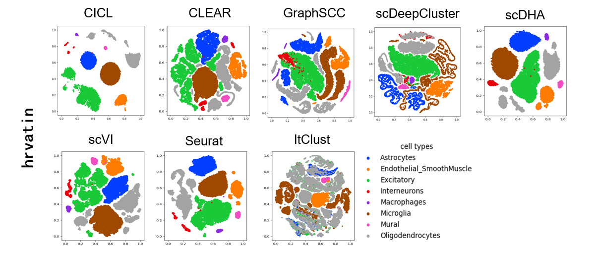
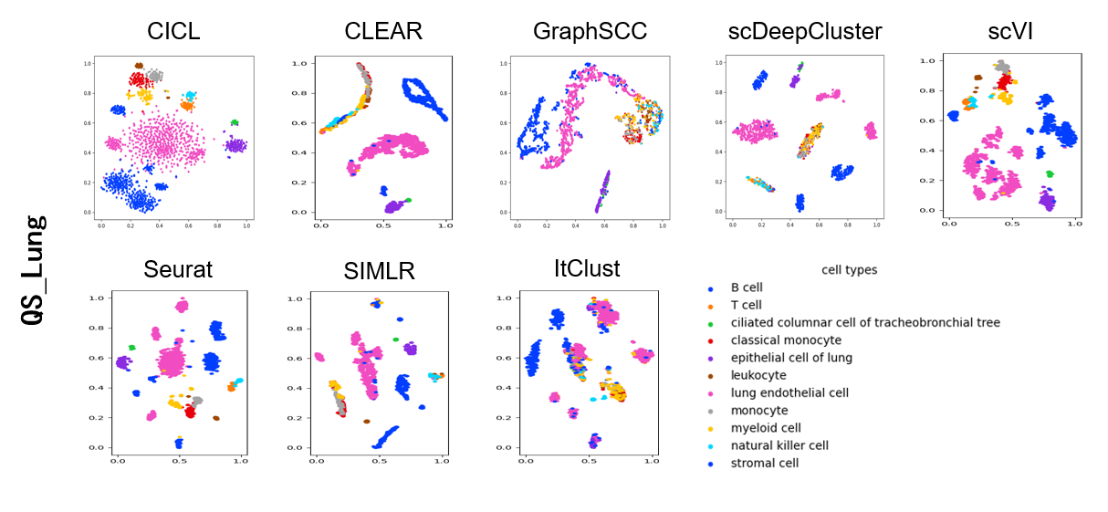
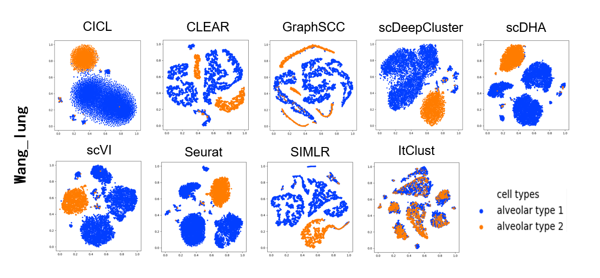
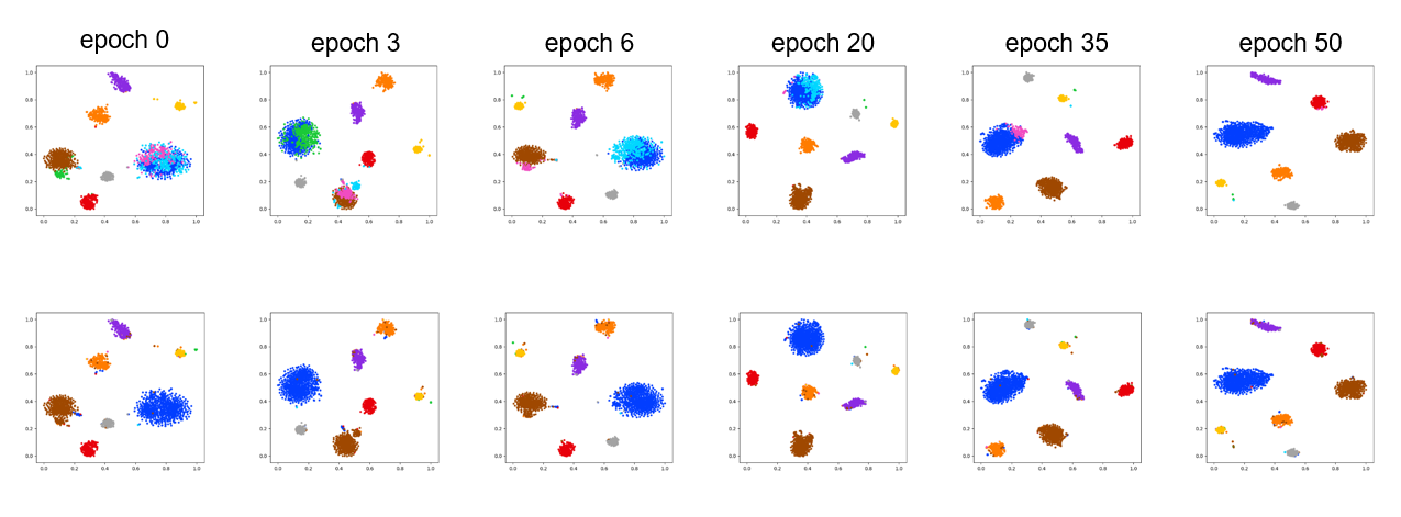
Fig. 3 illustrates the clustering process of our iterative contrastive learning on the muraro dataset. The upper and lower figures represent the clustering results of our method and the ground truth, respectively. We can see that various types of cells are distributed chaotically in the early epochs (e.g. epoch = 0, 3, 6). However, as the iterative learning goes, CICL split different types of cells with growing accuracy. At epoch 50, our method correctly clusters the data. In summary, CICL is able to gradually refine the clustering outcome, and eventually makes the clustering result match with the ground truth. This demonstrates that our model iteratively learns more and more accurate cell representations.

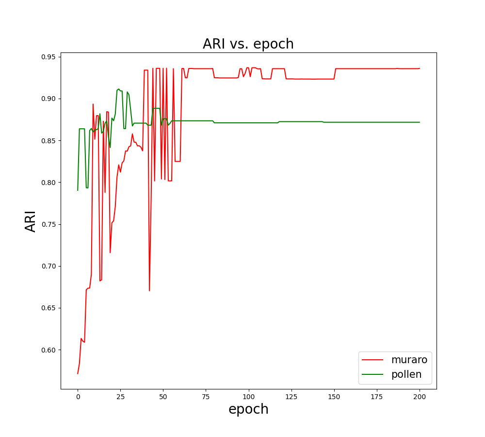
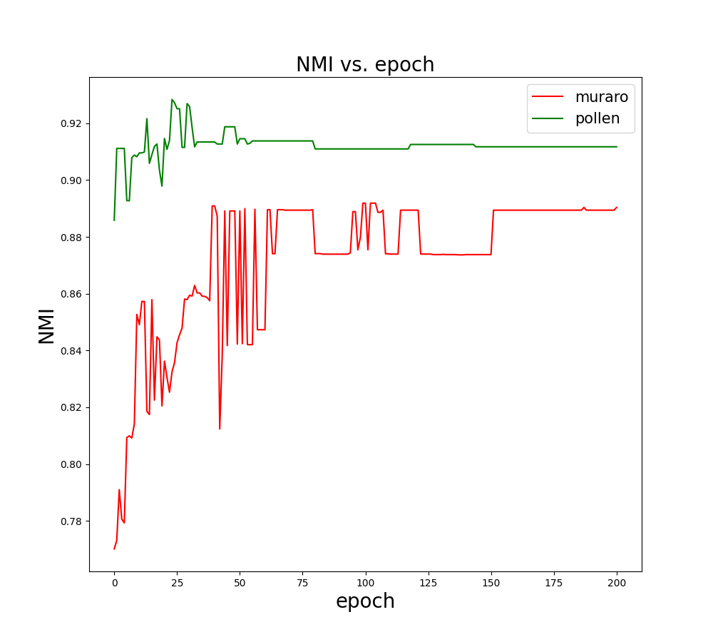
Furthermore, we demonstrate how the clustering performance metrics ARI and NMI change with the iterative contrastive learning process on the muraro and pollen datasets in Fig. 4. We can see that in the early epochs (epoch $<$60 on muraro and epoch $<$50 on pollen), both metrics undergo a rapid increasing and acutely fluctuation period. After that, the metrics enter a relatively stable period. Certainly, excessive training will also lead to overfitting and result in slight degradation of model performance, as we can see on the pollen dataset.

Fig. 3: Iterative clustering results on the muraro dataset, which show the visualization of embedded cells in the learning process. Upper: clustering results of our method; Lower: ground truth. Each color indicates a type of cells.

((1))

((2))

Fig. 4: The ARI and NMI results during the iterative learning process on the muraro and pollen datasets.

3.5 Ablation Study

Here, we conduct ablation studies on the effect of cluster-aware contrastive learning.

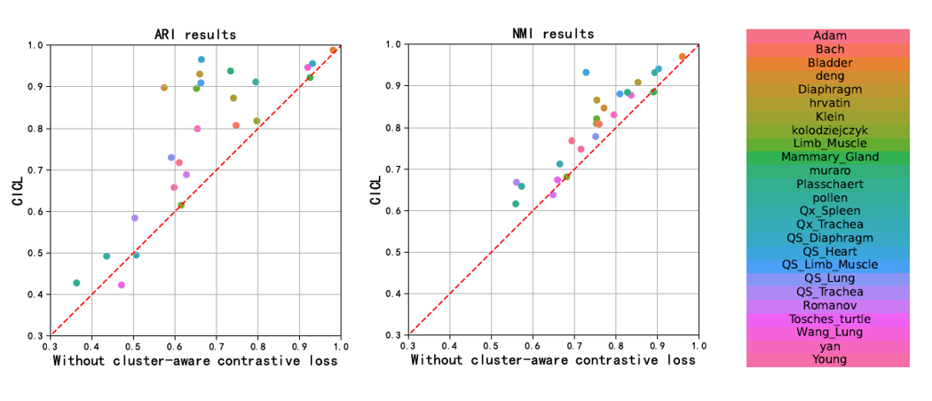
Cluster-aware contrastive loss. One of the major innovations of CICL is the cluster-aware contrastive learning mechanism, which incorporates cluster structure information into contrastive loss, thereby enhancing the representations of cells. To validate the effectiveness of our mechanism, we conduct an ablation study. For comparison, we consider a variant without the cluster-aware loss (i.e., the 2nd term in Equ. (17)). The results are presented in Fig. 5. Here, the vertical axis shows the results of our method, and the horizontal axis presents the results of the variant without the cluster-aware contrastive loss. Notably, in terms of both ARI and NMI, the majority of points lie above the line $y=x$, indicating that CICL outperforms the variant model, which affirms the efficacy of our new contrastive learning loss. Nevertheless, we also see that on some datasets (e.g. kolodziejczyk, Mammary_Gland and Tosches_turtle), CICL exhibits similar or even inferior performance. This is possibly caused by the errors of pseudo-labels.

Fig. 5: Comparison between CICL and a variant without the cluster-aware contrastive loss. Vertical axis indicates results of our method, and horizontal axis stands for the results of the variant model. Each point in the figures represents the result on a dataset. Points above the $y=x$ line indicate that our method outperforms the variant on the corresponding datasets.

Effect of hyperparameter $\lambda$. Here, we investigate the effect of the hyperparameter $\lambda$ on the performance of the model. We increase $\lambda$ from 0 to 1.0, and report the performance in terms of ARI and NMI. The results are illustrated in Fig. 6. We can see that our method has the worst performance at $\lambda=0$ (without the cluster-aware contrastive loss). As $\lambda$ increases, the performance is improved rapidly. When $\lambda=0.1$, both ARI and NMI reach the highest point. After that, ARI and NMI decrease slightly and gradually tend to be stable with the increase of $\lambda$. The result indicates that the model considerably benefits from the cluster-aware contrastive loss. In our experiments, we set $\lambda$=0.1, to avoid potential negative impact of pseudo-label error.

Fig. 6: The ARI and NMI results of CICL on muraro under different $\lambda$ values.

4 Conclusion

In this paper, to boost the performance of scRNA-seq data clustering analysis, we propose a novel approach called CICL. CICL adopts an iterative representation learning and clustering framework with an innovative cluster-aware contrastive loss. By comprehensively exploiting the underlying cluster structure of the training data, CICL can learn better scRNA-seq data presentations and thus achieve better clustering performance progressively. Extensive experiments on 25 real scRNA-seq datasets show that CICL outperforms the state-of-the-art methods in most cases, and achieves dominate advantage over the existing methods on average. Future work will focus on replacing K-means with advanced clustering methods to generate accurate pseudo-labels, and extending our idea to other downstream scRNA-seq data analysis tasks.

References

- Adam et al. [2017] Mike Adam, Andrew S Potter, and S Steven Potter. Psychrophilic proteases dramatically reduce single-cell rna-seq artifacts: a molecular atlas of kidney development. Development, 144(19):3625–3632, 2017.
- Bach et al. [2017] Karsten Bach, Sara Pensa, Marta Grzelak, James Hadfield, David J Adams, John C Marioni, and Walid T Khaled. Differentiation dynamics of mammary epithelial cells revealed by single-cell rna sequencing. Nature communications, 8(1):1–11, 2017.
- Blondel et al. [2008] Vincent D Blondel, Jean-Loup Guillaume, Renaud Lambiotte, and Etienne Lefebvre. Fast unfolding of communities in large networks. Journal of statistical mechanics: theory and experiment, 2008(10):P10008, 2008.
- Chen et al. [2020] Ting Chen, Simon Kornblith, Mohammad Norouzi, and Geoffrey Hinton. A simple framework for contrastive learning of visual representations. In International conference on machine learning, pages 1597–1607. PMLR, 2020.
- Ciortan and Defrance [2021] Madalina Ciortan and Matthieu Defrance. Contrastive self-supervised clustering of scrna-seq data. BMC bioinformatics, 22(1):280, 2021.
- Consortium [2020] Tabula Muris Consortium. A single-cell transcriptomic atlas characterizes ageing tissues in the mouse. Nature, 583(7817):590–595, 2020.
- Deng et al. [2014] Qiaolin Deng, Daniel Ramsköld, Björn Reinius, and Rickard Sandberg. Single-cell rna-seq reveals dynamic, random monoallelic gene expression in mammalian cells. Science, 343(6167):193–196, 2014.
- Deng et al. [2021] Weiwei Deng, Yubo Ma, Zhen Su, Yufang Liu, Panpan Liang, Chen Huang, Xiao Liu, Jin Shao, Yi Zhang, Kai Zhang, et al. Single-cell rna-sequencing analyses identify heterogeneity of cd8+ t cell subpopulations and novel therapy targets in melanoma. Molecular Therapy-Oncolytics, 20:105–118, 2021.
- Eraslan et al. [2019] Gökcen Eraslan, Lukas M Simon, Maria Mircea, Nikola S Mueller, and Fabian J Theis. Single-cell rna-seq denoising using a deep count autoencoder. Nature communications, 10(1):390, 2019.
- Flores et al. [2022] Mario Flores, Zhentao Liu, Tinghe Zhang, Md Musaddaqui Hasib, Yu-Chiao Chiu, Zhenqing Ye, Karla Paniagua, Sumin Jo, Jianqiu Zhang, Shou-Jiang Gao, et al. Deep learning tackles single-cell analysis—a survey of deep learning for scrna-seq analysis. Briefings in bioinformatics, 23(1):bbab531, 2022.
- Gan et al. [2022] Yanglan Gan, Xingyu Huang, Guobing Zou, Shuigeng Zhou, and Jihong Guan. Deep structural clustering for single-cell rna-seq data jointly through autoencoder and graph neural network. Briefings in Bioinformatics, 23(2):bbac018, 2022.
- Guo et al. [2017] Xifeng Guo, Long Gao, Xinwang Liu, and Jianping Yin. Improved deep embedded clustering with local structure preservation. In Ijcai, volume 17, pages 1753–1759, 2017.
- Han et al. [2022] Wenkai Han, Yuqi Cheng, Jiayang Chen, Huawen Zhong, Zhihang Hu, Siyuan Chen, Licheng Zong, Liang Hong, Ting-Fung Chan, Irwin King, et al. Self-supervised contrastive learning for integrative single cell rna-seq data analysis. Briefings in Bioinformatics, 23(5):bbac377, 2022.
- He et al. [2020] Kaiming He, Haoqi Fan, Yuxin Wu, Saining Xie, and Ross Girshick. Momentum contrast for unsupervised visual representation learning. In Proceedings of the IEEE/CVF conference on computer vision and pattern recognition, pages 9729–9738, 2020.
- Hrvatin et al. [2018] Sinisa Hrvatin, Daniel R Hochbaum, M Aurel Nagy, Marcelo Cicconet, Keiramarie Robertson, Lucas Cheadle, Rapolas Zilionis, Alex Ratner, Rebeca Borges-Monroy, Allon M Klein, et al. Single-cell analysis of experience-dependent transcriptomic states in the mouse visual cortex. Nature neuroscience, 21(1):120–129, 2018.
- Hu et al. [2020] Jian Hu, Xiangjie Li, Gang Hu, Yafei Lyu, Katalin Susztak, and Mingyao Li. Iterative transfer learning with neural network for clustering and cell type classification in single-cell rna-seq analysis. Nature machine intelligence, 2(10):607–618, 2020.
- Kiselev et al. [2019] Vladimir Yu Kiselev, Tallulah S Andrews, and Martin Hemberg. Challenges in unsupervised clustering of single-cell rna-seq data. Nature Reviews Genetics, 20(5):273–282, 2019.
- Klein et al. [2015] Allon M Klein, Linas Mazutis, Ilke Akartuna, Naren Tallapragada, Adrian Veres, Victor Li, Leonid Peshkin, David A Weitz, and Marc W Kirschner. Droplet barcoding for single-cell transcriptomics applied to embryonic stem cells. Cell, 161(5):1187–1201, 2015.
- Kolodziejczyk et al. [2015] Aleksandra A Kolodziejczyk, Jong Kyoung Kim, Jason CH Tsang, Tomislav Ilicic, Johan Henriksson, Kedar N Natarajan, Alex C Tuck, Xuefei Gao, Marc Bühler, Pentao Liu, et al. Single cell rna-sequencing of pluripotent states unlocks modular transcriptional variation. Cell stem cell, 17(4):471–485, 2015.
- Lopez et al. [2018] Romain Lopez, Jeffrey Regier, Michael B Cole, Michael I Jordan, and Nir Yosef. Deep generative modeling for single-cell transcriptomics. Nature methods, 15(12):1053–1058, 2018.
- Muraro et al. [2016] Mauro J Muraro, Gitanjali Dharmadhikari, Dominic Grün, Nathalie Groen, Tim Dielen, Erik Jansen, Leon Van Gurp, Marten A Engelse, Francoise Carlotti, Eelco Jp De Koning, et al. A single-cell transcriptome atlas of the human pancreas. Cell systems, 3(4):385–394, 2016.
- Oord et al. [2018] Aaron van den Oord, Yazhe Li, and Oriol Vinyals. Representation learning with contrastive predictive coding. arXiv preprint arXiv:1807.03748, 2018.
- Plasschaert et al. [2018] Lindsey W Plasschaert, Rapolas Žilionis, Rayman Choo-Wing, Virginia Savova, Judith Knehr, Guglielmo Roma, Allon M Klein, and Aron B Jaffe. A single-cell atlas of the airway epithelium reveals the cftr-rich pulmonary ionocyte. Nature, 560(7718):377–381, 2018.
- Pollen et al. [2014] Alex A Pollen, Tomasz J Nowakowski, Joe Shuga, Xiaohui Wang, Anne A Leyrat, Jan H Lui, Nianzhen Li, Lukasz Szpankowski, Brian Fowler, Peilin Chen, et al. Low-coverage single-cell mrna sequencing reveals cellular heterogeneity and activated signaling pathways in developing cerebral cortex. Nature biotechnology, 32(10):1053–1058, 2014.
- Romanov et al. [2017] Roman A Romanov, Amit Zeisel, Joanne Bakker, Fatima Girach, Arash Hellysaz, Raju Tomer, Alan Alpar, Jan Mulder, Frederic Clotman, Erik Keimpema, et al. Molecular interrogation of hypothalamic organization reveals distinct dopamine neuronal subtypes. Nature neuroscience, 20(2):176–188, 2017.
- Satija et al. [2015] Rahul Satija, Jeffrey A Farrell, David Gennert, Alexander F Schier, and Aviv Regev. Spatial reconstruction of single-cell gene expression data. Nature biotechnology, 33(5):495–502, 2015.
- Schaum et al. [2018] Nicholas Schaum, Jim Karkanias, Norma F Neff, Andrew P May, Stephen R Quake, Tony Wyss-Coray, Spyros Darmanis, Joshua Batson, Olga Botvinnik, Michelle B Chen, et al. Single-cell transcriptomics of 20 mouse organs creates a tabula muris: The tabula muris consortium. Nature, 562(7727):367, 2018.
- Stegle et al. [2015] Oliver Stegle, Sarah A Teichmann, and John C Marioni. Computational and analytical challenges in single-cell transcriptomics. Nature Reviews Genetics, 16(3):133–145, 2015.
- Tang et al. [2009] Fuchou Tang, Catalin Barbacioru, Yangzhou Wang, Ellen Nordman, Clarence Lee, Nanlan Xu, Xiaohui Wang, John Bodeau, Brian B Tuch, Asim Siddiqui, et al. mrna-seq whole-transcriptome analysis of a single cell. Nature methods, 6(5):377–382, 2009.
- Tian et al. [2019] Tian Tian, Ji Wan, Qi Song, and Zhi Wei. Clustering single-cell rna-seq data with a model-based deep learning approach. Nature Machine Intelligence, 1(4):191–198, 2019.
- Tosches et al. [2018] Maria Antonietta Tosches, Tracy M Yamawaki, Robert K Naumann, Ariel A Jacobi, Georgi Tushev, and Gilles Laurent. Evolution of pallium, hippocampus, and cortical cell types revealed by single-cell transcriptomics in reptiles. Science, 360(6391):881–888, 2018.
- Tran et al. [2021] Duc Tran, Hung Nguyen, Bang Tran, Carlo La Vecchia, Hung N Luu, and Tin Nguyen. Fast and precise single-cell data analysis using a hierarchical autoencoder. Nature communications, 12(1):1029, 2021.
- Van der Maaten and Hinton [2008] Laurens Van der Maaten and Geoffrey Hinton. Visualizing data using t-sne. Journal of machine learning research, 9(11), 2008.
- van Galen et al. [2019] Peter van Galen, Volker Hovestadt, Marc H Wadsworth II, Travis K Hughes, Gabriel K Griffin, Sofia Battaglia, Julia A Verga, Jason Stephansky, Timothy J Pastika, Jennifer Lombardi Story, et al. Single-cell rna-seq reveals aml hierarchies relevant to disease progression and immunity. Cell, 176(6):1265–1281, 2019.
- Vaswani et al. [2017] Ashish Vaswani, Noam Shazeer, Niki Parmar, Jakob Uszkoreit, Llion Jones, Aidan N Gomez, Łukasz Kaiser, and Illia Polosukhin. Attention is all you need. Advances in neural information processing systems, 30, 2017.
- Wan et al. [2022] Hui Wan, Liang Chen, and Minghua Deng. scname: neighborhood contrastive clustering with ancillary mask estimation for scrna-seq data. Bioinformatics, 38(6):1575–1583, 2022.
- Wang et al. [2018a] Bo Wang, Daniele Ramazzotti, Luca De Sano, Junjie Zhu, Emma Pierson, and Serafim Batzoglou. Simlr: A tool for large-scale genomic analyses by multi-kernel learning. Proteomics, 18(2):1700232, 2018a.
- Wang et al. [2018b] Yanjie Wang, Zan Tang, Huanwei Huang, Jiao Li, Zheng Wang, Yuanyuan Yu, Chengwei Zhang, Juan Li, Huaping Dai, Fengchao Wang, et al. Pulmonary alveolar type i cell population consists of two distinct subtypes that differ in cell fate. Proceedings of the National Academy of Sciences, 115(10):2407–2412, 2018b.
- Wolf et al. [2018] F Alexander Wolf, Philipp Angerer, and Fabian J Theis. Scanpy: large-scale single-cell gene expression data analysis. Genome biology, 19:1–5, 2018.
- Xie et al. [2016] Junyuan Xie, Ross Girshick, and Ali Farhadi. Unsupervised deep embedding for clustering analysis. In International conference on machine learning, pages 478–487. PMLR, 2016.
- Yan et al. [2013] Liying Yan, Mingyu Yang, Hongshan Guo, Lu Yang, Jun Wu, Rong Li, Ping Liu, Ying Lian, Xiaoying Zheng, Jie Yan, et al. Single-cell rna-seq profiling of human preimplantation embryos and embryonic stem cells. Nature structural & molecular biology, 20(9):1131–1139, 2013.
- Young et al. [2018] Matthew D Young, Thomas J Mitchell, Felipe A Vieira Braga, Maxine GB Tran, Benjamin J Stewart, John R Ferdinand, Grace Collord, Rachel A Botting, Dorin-Mirel Popescu, Kevin W Loudon, et al. Single-cell transcriptomes from human kidneys reveal the cellular identity of renal tumors. science, 361(6402):594–599, 2018.
- Zeng et al. [2020] Yuansong Zeng, Xiang Zhou, Jiahua Rao, Yutong Lu, and Yuedong Yang. Accurately clustering single-cell rna-seq data by capturing structural relations between cells through graph convolutional network. In 2020 IEEE International Conference on Bioinformatics and Biomedicine (BIBM), pages 519–522. IEEE, 2020.
- Žurauskienė and Yau [2016] Justina Žurauskienė and Christopher Yau. pcareduce: hierarchical clustering of single cell transcriptional profiles. BMC bioinformatics, 17:1–11, 2016.