Effects of magnetic field on the equation of state in curved spacetime of a neutron star

Abstract

Neutron stars are known to have strong magnetic fields reaching as high as $10^{15}$ Gauss, besides having strongly curved interior spacetime. So for computing an equation of state for neutron-star matter, the effect of magnetic field as well as curved spacetime should be taken into account. In this article, we compute the equation of state for an ensemble of degenerate fermions in the curved spacetime of a neutron star in presence of a magnetic field. We show that the effect of curved spacetime on the equation of state is relatively stronger than the effect of observed strengths of magnetic field. Besides, a thin layer containing only spin-up neutrons is shown to form at the boundary of a degenerate neutron star.

I Introduction

The astrophysical data suggest that the surface magnetic field of a typical neutron star is around $10^{11}-10^{13}$ Gauss, whereas the internal field strength can reach up to $10^{15}$ Gauss or even higher [1, 2, 3]. The dominant matter constituent of neutron stars are believed to be charge-less neutrons. However, they interact with a magnetic field through the non-minimal Pauli-Dirac gauge coupling due to their intrinsic magnetic moment. Therefore, the presence of a strong magnetic field is expected to play an important role in determining thermodynamic properties of matter present inside the neutron stars. At the same time, neutron stars are also expected to contain electrically charged particles like protons and electrons. These charged particles directly interact with a magnetic field and form the well-known Landau levels quantum mechanically. These Landau levels are bound states of charged particles. Therefore, it is important to study their roles in computation of the fermionic degeneracy pressure which makes compact stars such as neutron stars stable against the gravitational collapse. The thermodynamic properties of a gas of charged particles under an external magnetic field in the Minkowski spacetime, have been studied earlier in [4, 5, 6].

However, recent articles [7, 8] show that the curved background geometry of a neutron star also plays a crucial role in determining the properties of the equation of state (EOS) of the matter present inside the star. In particular, metric-dependent gravitational time-dilation effect leads to an enhancement of the stiffness of the EOS of matter. Consequently, such an EOS, referred to as the curved EOS, leads to an enhancement of the mass limits of neutron stars [8]. We have mentioned that the observed neutron stars are known to have strong magnetic fields. Therefore, it is important to take the magnetic field into account while computing the EOS for a neutron star in its curved spacetime.

The key idea that we use for computing the EOS here is the lesson from Einstein’s general relativity that even in a curved spacetime one can always find a set of local coordinates in which the spacetime metric appears to be locally flat. However, it is unlike the usage of a globally flat spacetime which is commonly used in the literature to compute the EOS, referred to as the flat EOS, for neutron stars. Subsequently, we employ the methods of thermal quantum field theory to compute the EOS, as pioneered by Matsubara [9]. The result derived here shows that for an ensemble of charge-less neutrons the magnetic field and the gravitational time-dilation both leads the EOS to become stiffer whereas for an ensemble of charged fermions the magnetic field makes the EOS softer due to formation of the Landau levels. However, the changes of stiffness of the EOS due to the gravitational time dilation effect is relatively stronger than the changes due to the observed strengths of magnetic field.

II Interior spacetime

In the presence of an axial magnetic field, the interior spacetime of a neutron star can be modelled by an axially symmetric spacetime. On the other hand, the spacetime metric of a slowly rotating star that preserve axial symmetry can be represented, in the natural units $c=\hbar=1$, by the following invariant line element [10, 11]

$$ds^{2}=-e^{2\Phi}dt^{2}+e^{2\nu}dr^{2}+r^{2}[d\theta^{2}+\sin^{2}\theta(d\varphi-\omega dt)^{2}]~{},$$ (1)

where $\omega=\omega(r)$ is the acquired angular velocity of a freely-falling observer from infinity, a phenomena referred to as the dragging of inertial frames. On the other hand, the radial variation of the metric function $\Phi=\Phi(r)$ leads to the phenomena of gravitational time dilation. We note that in absence of the frame-dragging angular velocity $\omega$, the spacetime metric (1) represents a spherically symmetric spacetime.

The contribution of inertial frame-dragging on the EOS is controlled by a dimensionless ratio $(\omega/m)$ and if we consider $m$ to be the mass of neutrons then even for a rapidly rotating millisecond pulsar the dimensionless ratio is vanishingly small as $(\omega/m)\sim 10^{-22}$ [12]. Nevertheless, similar to the magnetic field $B$, the frame-dragging angular velocity $\omega$ couples to the spin-component of the Dirac field. However, as we have argued that the effect of inertial frame-dragging on the EOS is extremely small. So for computation of the EOS in the presence of a magnetic field, we neglect the inertial frame-dragging and we take into account only the effect of gravitational time-dilation, by considering the following invariant line element

$$ds^{2}=-e^{2\Phi}dt^{2}+e^{2\nu}dr^{2}+r^{2}[d\theta^{2}+\sin^{2}\theta d\varphi^{2}]~{},$$ (2)

which essentially represents a spherically symmetric spacetime.

III Anisotropic Pressure due to Magnetic field

In order to study the interior spacetime, here we consider the stellar matter to be described by a perfect fluid with the stress-energy tensor

$$T^{M}_{\mu\nu}=(\rho+P)u_{\mu}u_{\nu}+Pg_{\mu\nu}~{},$$ (3)

where $u^{\mu}$ is the 4-velocity of the stellar fluid satisfying $u_{\mu}u^{\mu}=-1$, $\rho$ is the energy density and $P$ is the pressure of the fluid. On the other hand, the stress-energy tensor associated with the electromagnetic field is given by

$$T^{E}_{\mu\nu}=\frac{1}{\mu_{0}}\left[F_{\mu\alpha}F_{\ \nu}^{\alpha}-\frac{1}{4}g_{\mu\nu}F_{\alpha\beta}F^{\alpha\beta}\right]~{},$$ (4)

where $\mu_{0}$ is the magnetic permeability of vacuum and $F_{\mu\nu}=\partial_{\mu}\mathcal{A}_{\nu}-\partial_{\nu}\mathcal{A}_{\mu}$ is the electromagnetic field tensor whose indices are contracted with respect to the spacetime metric. Therefore, the total stress-energy tensor $T_{\mu\nu}=T^{M}_{\mu\nu}+T^{E}_{\mu\nu}$, can be expressed in the following form

$$T_{\ \nu}^{\mu}=\text{diag}(-\rho,P_{r},P_{t},P_{t})~{}.$$ (5)

We note that due to the presence of a magnetic field the total radial pressure $P_{r}$ and total tangential pressure $P_{t}$ differ from each other. On the other hand total energy density $\rho$ now includes the contributions from both stellar fluid as well as from the magnetic field. The $tt$ and $rr$ components of Einstein’s equation $G_{\ \nu}^{\mu}=8\pi GT_{\ \nu}^{\mu}$ corresponding to the metric (2), lead to the following equations

$$\begin{split}8\pi Gr^{2}\rho&=e^{-2\nu}(2r\nu^{\prime}-1)+1~{},\\ 8\pi Gr^{2}P_{r}&=e^{-2\nu}(2r\Phi^{\prime}+1)-1~{}.\end{split}$$ (6)

By considering $e^{2\nu}=1/(1-2G\mathcal{M}/r)$, we obtain the equations

$$\frac{d\Phi}{dr}=\frac{G(\mathcal{M}+4\pi r^{3}P_{r})}{r(r-2G\mathcal{M})}~{}~{},~{}~{}\frac{d\mathcal{M}}{dr}=4\pi r^{2}\rho~{}.$$ (7)

The conservation of stress-energy tensor leads to the equation as follows

$$\frac{dP_{r}}{dr}=\frac{2}{r}(P_{t}-P_{r})-(P_{r}+\rho)\frac{d\Phi}{dr}~{}.$$ (8)

Additionally, we also have a second-order differential equation which follows from $G_{\ \theta}^{\theta}=8\pi GT_{\ \theta}^{\theta}$ equation and is given by

$$8\pi G\ P_{t}=e^{-2\nu}\Big{[}\frac{d^{2}\Phi}{dr^{2}}-\frac{d\Phi}{dr}\frac{d\nu}{dr}+\left(\frac{d\Phi}{dr}\right)^{2}+\frac{1}{r}\left(\frac{d\Phi}{dr}-\frac{d\nu}{dr}\right)\Big{]}~{}.$$ (9)

However, we note that the equation (9) is not an independent equation and it can be obtained from the conservation equation and $rr$-component of Einstein’s equation.

For a detailed study on the anisotropic spherical star in general relativity, see [13]. Nevertheless, we note that for an axial magnetic field $B$, the pressure components $P_{t}$ and $P_{r}$ would differ from each other by the terms of $\mathcal{O}(B^{2})$. So for the cases where $\mathcal{O}(B^{2})$ terms are negligible, the total pressure can be considered to be isotropic. We shall see later that the observed field strength of even $10^{15}$ Gauss is significantly smaller compared to the characteristic field strength $B_{c}\approx 10^{20}$ Gauss associated with the nucleons. It allows us to neglect the terms of $\mathcal{O}(B^{2})$ which in turn permits the exterior metric to be described by the Schwarzschild metric such that metric function $\Phi$ is subject to the boundary condition $e^{2\Phi(R)}=1-2GM/R$. For a typical neutron star having mass $M=1M_{\odot}$ and radius $R=10$ km, the metric function $\Phi(R)\simeq-0.17$. Further, it follows from the equation (7) that the values of $\Phi$ inside the star are lower than $\Phi(R)$ as $(d\Phi/dr)$ is positive definite.

IV Local thermal equilibrium

Due to the hydrostatic equilibrium, the thermodynamic properties such as the pressure, the energy density vary radially inside a star. On the other hand, these thermodynamic properties are required to be uniform within a given thermodynamical system in equilibrium. Nevertheless, these two seemingly disparate aspects can be reconciled by introducing the concept of local thermodynamical equilibrium inside the star.

In order to ensure the conditions for local thermodynamic equilibrium inside a star, we can choose a sufficiently small region but containing large number of degrees of freedom. Inside this small region the metric variations can be neglected. For definiteness, we chose a box-shaped small region whose center is located at say $r=r_{0}$. By following the coordinate transformations given in [7], namely $x=e^{\nu(r_{0})}r\sin\bar{\theta}\cos\phi$, $y=e^{\nu(r_{0})}r\sin\bar{\theta}\sin\phi$, and $z=e^{\nu(r_{0})}r\cos\bar{\theta}$ along with $\bar{\theta}=e^{-\nu(r_{0})}\theta$ for small $\theta$, we can reduce the metric (2) to the following form

$$ds^{2}=-e^{2\Phi(r_{0})}dt^{2}+dx^{2}+dy^{2}+dz^{2},$$ (10)

in a locally Cartesian coordinates. The metric within the box (10) contains the information about the metric function $\Phi=\Phi(r_{0})$, in contrast to the usage of a globally flat spacetime for computing the matter EOS in the literature [14, 15, 16, 17, 18, 19]. The metric function $\Phi$ is treated here as a constant within the scale of the box, which is sufficient to describe the microscopic physics of the constituent particles. However, the metric function $\Phi$ varies at the scale of the star, as governed by the equations (7).

V Neutrons in an external magnetic field

Neutrons are electrically neutral particles, hence, they do not couple minimally to the gauge field associated with the external magnetic field. However, neutrons possess a magnetic dipole moment due to their internal quark degrees of freedom. Consequently, under an external magnetic field, neutrons couple to the gauge field non-minimally through the Pauli-Dirac interaction. The corresponding action is given by

$$S=-\int\sqrt{-g}d^{4}x\bar{\psi}\Big{[}ie_{\ a}^{\mu}\gamma^{a}\mathcal{D}_{\mu}+m-\frac{{\bf\mu_{D}}}{2}\sigma^{\mu\nu}F_{\mu\nu}\Big{]}\psi~{},$$ (11)

where spinor field $\psi$ represents the neutrons with mass $m$ and $\bar{\psi}=\psi^{\dagger}\gamma^{0}$ being its Dirac adjoint. The tetrad components ${e^{\mu}}_{a}$ are defined as $g_{\mu\nu}{e^{\mu}}_{a}{e^{\nu}}_{b}=\eta_{ab}$ where $g_{\mu\nu}$ is the spacetime metric whereas $\eta_{ab}=diag(-1,1,1,1)$ is the Minkowski metric. The spin-covariant derivative is defined as $\mathcal{D}_{\mu}\psi\equiv\partial_{\mu}\psi+\Gamma_{\mu}\psi$ where spin connection $\Gamma_{\mu}$ is given by

$$\Gamma_{\mu}=-\tfrac{1}{8}\eta_{ac}{e_{\nu}}^{c}(\partial_{\mu}{e^{\nu}}_{b}+\Gamma^{\nu}_{\mu\sigma}{e^{\sigma}}_{b})~{}[\gamma^{a},\gamma^{b}]~{},$$ (12)

with $\Gamma^{\nu}_{\mu\beta}$ being the Christoffel connections. The Dirac matrices $\gamma^{a}$ satisfy the Clifford algebra $\{\gamma^{a},\gamma^{b}\}=-2\eta^{ab}\mathbb{I}$ together with the relations $(\gamma^{0})^{2}=\mathbb{I}$ and $(\gamma^{k})^{2}=-\mathbb{I}$ for $k=1,2,3$. In the Pauli-Dirac interaction term, ${\bf\mu_{D}}$ denotes the magnitude of magnetic moment of neutrons and $\sigma^{\mu\nu}=\frac{i}{2}{e^{\mu}}_{a}{e^{\nu}}_{b}[\gamma^{a},\gamma^{b}]$.

V.1 Partition function

In order to compute the partition function around a given a point inside the star, we consider a small region around it where the metric can be reduced to the form (10). Within this box-shaped region the tetrad components can be expressed as $e_{\ 0}^{t}=e^{-\Phi},\ e_{\ 1}^{x}=e_{\ 2}^{y}=e_{\ 3}^{z}=1$. Consequently, the spin-connection within the box vanishes i.e. $\Gamma_{\mu}=0$. Additionally, we choose the magnetic field to be in the $z$-direction with its field strength being $B$. For such a magnetic field the gauge field components can be chosen as $\mathcal{A}_{\mu}=(0,0,Bx,0)$. Therefore, within the Box, the action (11) reduces to the following form

$$S=-\int d^{4}x\bar{\psi}\Big{[}i\gamma^{0}\partial_{t}+e^{\Phi}(i\gamma^{k}\partial_{k}+m)-e^{\Phi}{\bf\mu_{D}}B\Sigma_{3}\Big{]}\psi~{},$$ (13)

where $\Sigma_{3}=\tfrac{i}{2}[\gamma^{1},\gamma^{2}]=\sigma_{3}\otimes\mathbb{I}_{2}$ and $\sigma_{3}$ is the Pauli matrix associated with the spin operator along $z$-direction.

In functional integral approach, the partition function can be expressed as $\mathcal{Z}=\int\mathcal{D}\bar{\psi}\mathcal{D}\psi\ e^{-S^{\beta}}$ by using the coherent states of the Grassmann fields [20, 21, 22]. Here $S^{\beta}$ denotes the Euclidean action obtained obtained through the Wick rotation $t\rightarrow-i\tau$. By following the approach as given in [7, 12], we can express the Euclidean action as

$$S^{\beta}=\int_{0}^{\beta}d\tau\int d^{3}x\bar{\psi}\big{[} - \gamma^{0}(\partial_{\tau}+\mu+e^{\Phi}{\bf\mu_{D}}B\gamma^{0}\Sigma_{3})$$ (14)

$$+ e^{\Phi}(i\gamma^{k}\partial_{k}+m)\big{]}\psi.$$

The equilibrium temperature $T$ of the system leads to the following anti-periodic boundary condition on the Dirac field

$$\psi(\tau,\mathbf{x})=-\psi(\tau+\beta,\mathbf{x})~{},$$ (15)

where $\beta=1/(k_{B}T)$ with $k_{B}$ being the Boltzmann constant. By using the Matsubara frequencies $\omega_{l}=(2l+1)\pi/\beta$ where $l$ is an integer, we can express the field $\psi$ in the Fourier domain as

$$\psi(\tau,\mathbf{x})=\frac{1}{\sqrt{V}}\sum_{l,\mathrm{k}}~{}e^{-i(\omega_{l}\tau+\mathrm{k}\cdot\mathbf{x})}\tilde{\psi}(l,\mathrm{k})~{},$$ (16)

where volume of the box is now $V=\int d^{3}x\sqrt{-\eta}$. The equation (16) then leads the action (14) to become

$$S^{\beta}=\sum_{l,\mathrm{k}}~{}\bar{\tilde{\psi}}~{}\beta\left[\not{p}+\bar{m}\right]\tilde{\psi}~{},$$ (17)

where $\not{p}=\gamma^{0}(i\omega_{l}-\mu-e^{\Phi}{\bf\mu_{D}}B\gamma^{0}\Sigma_{3})+\gamma^{k}(\mathrm{k}_{k}e^{\Phi})$ and $\bar{m}=me^{\Phi}$. Using the results of Gaussian integral over the Grassmann fields and the Dirac representation of $\gamma^{a}$ matrices, one can evaluate the partition function $\mathcal{Z}$ for the particle sector as

$$\ln\mathcal{Z}=\sum_{s=\pm}\sum_{\mathrm{k}}\ln\left(1+e^{\beta(\mu_{s}-\varepsilon)}\right)~{},$$ (18)

where $\varepsilon^{2}=\varepsilon(\mathrm{k})^{2}=e^{\Phi}(\mathrm{k}^{2}+m^{2})$ and the modified chemical potential associated with the different spins of neutrons are

$$\mu_{s}=\mu+se^{\Phi}{\bf\mu_{D}}B~{}.$$ (19)

In general, the presence of a magnetic field makes the dispersion relation anisotropic in the momentum space. As a result, the Fermi-surface is no longer spherical in nature, rather it becomes an ellipsoid. However, for $({\bf\mu_{D}}B/m)\ll 1$ limit (which is typically the case inside a neutron star) and neglecting the anisotropy due to the fact $(k_{z}/m)\ll 1$, we get the following two dispersions

$$\omega=e^{\Phi}(\varepsilon\pm{\bf\mu_{D}}B)~{},$$ (20)

which are two shifted spheres. In the thermodynamic limit, the summation over $\mathrm{k}$ in the equation (18) can be expressed as an integral over the momentum space that results in the following expression of the partition function

$$\ln\mathcal{Z}=\sum_{s=\pm}\frac{e^{-3\Phi}\beta V}{48\pi^{2}}\Big{[}2\mu_{s}\mu_{sm}^{3}-3\bar{m}^{2}\bar{\mu}_{sm}^{2}\Big{]}~{},$$ (21)

where $\mu_{sm}=\sqrt{\mu_{s}^{2}-\bar{m}^{2}}$ and $\bar{\mu}_{sm}^{2}=\mu_{s}\mu_{sm}-\bar{m}^{2}\operatorname{asinh}(\mu_{sm}/\bar{m})$. In arriving at the expression (21), we have neglected the temperature corrections of $\mathcal{O}((\beta\mu)^{-2})$, given a degenerate star is characterized by the condition $(\beta\mu)\gg 1$. Additionally, we have omitted formally divergent zero-point energy terms.

V.2 Pressure and energy density

We can compute number density of neutrons from the partition function (21) as $n=(\beta V)^{-1}(\partial\ln\mathcal{Z})/(\partial\mu)$ which leads to

$$n=n_{+}+n_{-}~{},~{}~{}\text{with}~{}~{}n_{\pm}=\frac{e^{-3\Phi}}{6\pi^{2}}\mu_{\pm m}^{3}~{}.$$ (22)

The equation (22) can be used to express the modified chemical potentials in terms of the number densities of spin-up and spin-down neutrons respectively as $\mu_{\pm}=me^{\Phi}\sqrt{(bn_{\pm})^{2/3}+1}$ where $b=(6\pi^{2})/m^{3})$. We should mention here that $\mu_{\pm}$ can be equivalently treated as independent variables in places of $\mu$ and $B$. The equation (19) then leads to the following relation

$$\sqrt{(bn_{+})^{2/3}+1}-\sqrt{(bn_{-})^{2/3}+1}=2\left(\frac{B}{B_{c}}\right)~{},$$ (23)

where the constant $B_{c}=(m/{\bf\mu_{D}})\approx 10^{20}$ Gauss. The constant $B_{c}$ here signifies the characteristic scale of magnetic field associated with neutrons.

For a grand canonical ensemble, we can compute total pressure from the partition function (21) as $P=(\beta V)^{-1}\ln\mathcal{Z}=P_{+}+P_{-}$ where the pressure components associated with the different spins of neutrons are

$$P_{\pm}=e^{\Phi}\frac{m^{4}}{48\pi^{2}} \left[\sqrt{(bn_{\pm})^{2/3}+1}\left\{2(bn_{\pm})-3(bn_{\pm})^{1/3}\right\}\right.$$ (24)

$$+\left.~{}3\operatorname{asinh}\left\{(bn_{\pm})^{1/3}\right\}\right]~{}.$$

For the metric (10), the 4-velocity vector in the box corresponding to the perfect fluid form of the stellar fluid (3) can be expressed as $u^{\mu}=e^{-\Phi}(1,0,0,0)$ along with its co-vector $u_{\mu}=e^{\Phi}(-1,0,0,0)$. Consequently, the energy density $\rho$ can be expressed in terms of the partition function as $(\rho-\mu n)V=-(\partial\ln\mathcal{Z}/\partial\beta)$ [12] leading to $\rho=\rho_{+}+\rho_{-}$ where

$$\rho_{\pm}=-P_{\pm}+e^{\Phi}\frac{m^{4}}{6\pi^{2}}(bn_{\pm})\sqrt{(bn_{\pm})^{2/3}+1}~{}.$$ (25)

In the limit $B\to 0$, we note that $\mu_{+}=\mu_{-}$. Consequently, in this limit total pressure $P$ and total energy density $\rho$ reduce to the expressions of pressure and energy density for an ensemble of non-interacting degenerate neutrons as expected. For a non-zero $B$, it can be checked that the corrections to the total pressure $P$ and total energy density $\rho$ are of $\mathcal{O}(B^{2})$.

The behaviour of total pressure as a function of number density for different values of the magnetic field and the metric function is plotted in the FIG. 1. On the other hand, the FIG. 2 shows the behaviour of pressure, energy density ratio as a function of energy density and it shows the stiffening of the EOS due to the effects of both magnetic field and gravitational time dilation.

Figure 1: Plot of the pressure $P$ exerted by an ensemble of non-interacting degenerate neutrons under an external magnetic field $B$ as a function of neutron number density $n$ for different kinematical values of metric function $\Phi$. The curves $2$ and $3$ with different plausible values of magnetic field $B$ are nearly indistinguishable. The change of pressure due to the magnetic field $B$ i.e. $\Delta P\equiv P_{B}-P_{B=0}$ is shown in the inset plot using same units as the main plot. It shows that effect of magnetic field on the pressure is rather small. In contrast, the effect of gravitational time-dilation on the pressure, described by $\Phi$, is considerably large.

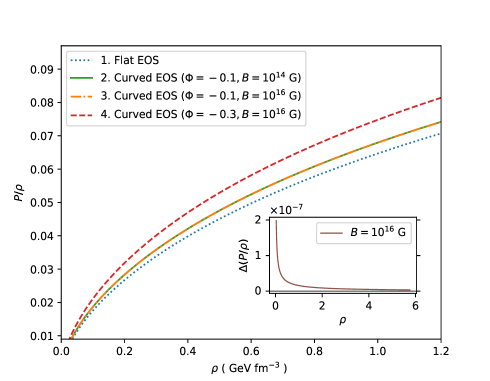
Figure 2: Plot of the ratio $P/\rho$ as a function of energy density $\rho$ for different values of magnetic field $B$ and metric function $\Phi$. As earlier, the curves $2$ and $3$ with different values of magnetic field $B$ are nearly indistinguishable. The change of the ratio $P/\rho$ due to the magnetic field $B$ i.e. $\Delta(P/\rho)\equiv(P/\rho)_{B}-(P/\rho)_{B=0}$ is shown in the inset plot using same unit for $\rho$ as the main plot. As earlier, we note that the effect of gravitational time-dilation on the EOS is relatively stronger compared to the effect of an external magnetic field. Nevertheless, the EOS here becomes stiffer due to the effects of both the gravitational time-dilation and an external magnetic field.

V.3 Magnetic moment of a neutron star

We note from the equation (23) that for a non-zero value of magnetic field $B$, there is a population difference between different spins of neutrons. As a result, number densities of spin-up and spin-down neutrons, $n_{+}$ and $n_{-}$ respectively, cannot vanish simultaneously at the boundary of the star, and namely, $n_{-}$ vanishes earlier inside the neutron star. In particular, when $n_{-}$ becomes zero then we obtain

$$n_{+}=\frac{8}{b}\left[\frac{B}{B_{c}}\left(1+\frac{B}{B_{c}}\right)\right]^{3/2}~{}.$$ (26)

Consequently, due to the presence of a magnetic field there exists a thin layer at the boundary of a degenerate neutron star which contains only spin-up neutrons. In turn, the neutron star as a whole would acquire a net magnetic moment which would then naturally lead to an accretion of charge particles surrounding the neutron star. In the case of rotating neutron stars, analogous thin layer containing only one kind of spins has been reported earlier [23] where it arises due to the dragging of inertial frames.

VI Charged fermions in an external magnetic field

We have mentioned earlier that primary constituents of a neutron star are believed to be neutrons. However, a neutron star is also expected to have a smaller fraction of electrically charged fermions such as protons and electrons. Unlike neutrons, charged fermions couple minimally with the gauge field associated with an external magnetic field. We shall, however, ignore the contributions from the electromagnetic self-interaction between these fermions, as those are expected to be small [24]. The generally invariant action for an electrically charged Dirac fermion $\psi$ coupled to an electromagnetic gauge field $\mathcal{A}_{\mu}$ is given by

$$S=-\int\sqrt{-g}d^{4}x\bar{\psi}\Big{[}ie_{\ a}^{\mu}\gamma^{a}(\mathcal{D}_{\mu}-ie\mathcal{A}_{\mu})+m\Big{]}\psi~{},$$ (27)

where $e$ denotes the electrical charge of the fermion.

VI.1 Partition function

In order to evaluate the partition function, as earlier, we consider the external magnetic field to be along the $z$-direction and we choose the gauge field components to be $\mathcal{A}_{\mu}=(0,0,Bx,0)$. Therefore, within the box with the metric (10), we can reduce the Dirac action (27) to the following form

$$S=-\int d^{4}x\bar{\psi}\Big{[}i\gamma^{0}\partial_{t}+e^{\Phi}(i\gamma^{k}\partial_{k}+m)+e^{\Phi}\gamma^{2}eBx\Big{]}\psi~{}.$$ (28)

As earlier, the partition function can be expressed as $\mathcal{Z}=\int\mathcal{D}\bar{\psi}\mathcal{D}\psi\ e^{-S^{\beta}}$ where $S^{\beta}$ denotes the Euclidean action corresponding to the action (28) and is given by

$$S^{\beta}=\int_{0}^{\beta}d\tau\int d^{3}x\bar{\psi}\big{[} - \gamma^{0}(\partial_{\tau}+\mu)+e^{\Phi}(i\gamma^{k}\partial_{k}+m)$$ (29)

$$+ e^{\Phi}\gamma^{2}eBx\big{]}\psi~{}.$$

At thermal equilibrium, the Dirac field is subject to the anti-periodic boundary condition $\psi(\tau,\mathbf{x})=-\psi(\tau+\beta,\mathbf{x})$ leading to the Matsubara frequencies $\omega_{l}=(2l+1)\pi/\beta$ where $l$ is an integer. Therefore, we can express the field $\psi$ in the Fourier domain as

$$\psi(\tau,\mathbf{x})=\frac{1}{\sqrt{L_{y}L_{z}}}\sum_{l,k_{y},k_{z}}~{}e^{-i(\omega_{l}\tau+k_{y}y+k_{z}z)}\psi_{l}(x,k_{y},k_{z})~{},$$ (30)

where $L_{y}$ and $L_{z}$ denote the length of the box in the $y$ and $z$ directions respectively. The equations (29, 30) then lead to

$$S^{\beta}=\sum_{l,k_{y},k_{z}}\int dx~{}\bar{\psi_{l}}~{}\beta\left[\tilde{\not{\mathcal{D}}}+\bar{m}\right]\psi_{l}~{},$$ (31)

where $\tilde{\not{\mathcal{D}}}\equiv\gamma^{a}\tilde{\mathcal{D}}_{a}$ with

$$\tilde{\not{\mathcal{D}}}=\gamma^{0}(i\omega_{l}-\mu)+\gamma^{1}(ie^{\Phi}\partial_{x})+\gamma^{2}e^{\Phi}(eBx+k_{y})+\gamma^{3}e^{\Phi}k_{z}~{}.$$ (32)

The partition function then can be expressed as

$$\mathcal{Z}=\prod_{l,k_{y},k_{z}}\text{det}[\beta(\tilde{\not{\mathcal{D}}}+\bar{m})]~{}.$$ (33)

By using the property $\text{det}[\beta(\tilde{\not{\mathcal{D}}}+\bar{m})]=\text{det}[\gamma^{5}\beta(\tilde{\not{\mathcal{D}}}+\bar{m})\gamma^{5}]=\text{det}[\beta(-\tilde{\not{\mathcal{D}}}+\bar{m})]$ where $\gamma^{5}\equiv i\gamma^{0}\gamma^{1}\gamma^{2}\gamma^{3}$, $(\gamma^{5})^{2}=\mathbb{I}$ and $\{\gamma^{5},\gamma^{a}\}=0$, one can show that

$$\text{det}[\beta(\tilde{\not{\mathcal{D}}}+\bar{m})]=\text{det}[\beta^{2}(-\tilde{\not{\mathcal{D}}}^{2}+\bar{m}^{2})]^{1/2}~{}.$$ (34)

Using the properties of the $\gamma^{a}$ matrices, we can express

$$-\tilde{\not{\mathcal{D}}}^{2}+\bar{m}^{2}=(\omega_{l}+i\mu)^{2}+e^{2\Phi}\left[H_{xy}-eB\Sigma_{3}+k_{z}^{2}+m^{2}\right]~{},$$ (35)

where $\Sigma_{3}=\tfrac{i}{2}[\gamma^{1},\gamma^{2}]=\sigma_{3}\otimes\mathbb{I}_{2}$ and

$$H_{xy}=-\partial_{x}^{2}+(eB)^{2}\left(x+\frac{k_{y}}{eB}\right)^{2}~{}.$$ (36)

In order to evaluate the partition function (33) we can compute the trace over the eigenstates of the operator $\Sigma_{3}$ with eigenvalues $2s$ where $s=\pm\tfrac{1}{2}$ and of the operator $H_{xy}$ with eigenvalues $(2n+1)|eB|$ where $n$ being non-negative integers. It leads to

$$\ln\mathcal{Z}=\sum_{l,k_{y},k_{z},s,n}\ln\left[\beta^{2}\{(\omega_{l}+i\mu)^{2}+\varepsilon^{2}\}\right]~{},$$ (37)

where

$$\varepsilon^{2}=e^{2\Phi}\left[eB(2n+1-2s)+k_{z}^{2}+m^{2}\right]~{}.$$ (38)

In the equation (38), for brevity of notation, the term $|eB|$ is expressed as $eB$ and we shall use this notation henceforth. One can carry out the summation over Matsubara frequencies $\omega_{l}$ (see [7, 12]) which leads to the following expression of the partition function

$$\ln\mathcal{Z}=\sum_{k_{y},k_{z},s,n}\left[\ln\big{(}1+e^{-\beta(\varepsilon-\mu)}\big{)}+\ln\big{(}1+e^{-\beta(\varepsilon+\mu)}\big{)}\right]~{}.$$ (39)

In order to arrive at the equation (39), formally divergent terms such as the zero-point energy of fermions have been omitted. The first and the second terms in the equation (39) denotes the contributions from the particle and the anti-particle sectors respectively. Henceforth, we shall consider only the particle sector.

In the equation (38), we note that $\varepsilon$ is independent of $k_{y}$. However, in the equation (36), $k_{y}$ shifts the origin of $x$-coordinate. Therefore, for a system of charged fermions in the given box, we must require $|k_{y}/eB|\leq L_{x}/2$. By using the approximation $\sum_{k_{y},k_{z}}=(L_{y}L_{z})/(2\pi)^{2}\int dk_{y}dk_{z}$, we can express the partition function for the particle sector as

$$\ln\mathcal{Z}=\frac{eBV}{4\pi^{2}}\sum_{s,n}\int dk_{z}\ln\big{(}1+e^{-\beta(\varepsilon-\mu)}\big{)}~{},$$ (40)

where $V$ being the volume of the box. We note that in the partition function (40), we can replace the summation over the index $s$ and $n$ by a single summation over an index $\ell$ as follows

$$\ln\mathcal{Z}=\ln\mathcal{Z}_{0}+2\sum_{\ell=1}\ln\mathcal{Z}_{\ell}~{},$$ (41)

where

$$\ln\mathcal{Z}_{\ell}=\frac{eBV}{2\pi^{2}}\int_{0}^{\infty}dk\ln\big{(}1+e^{-\beta(\varepsilon_{\ell}-\mu)}\big{)}~{},$$ (42)

with $\varepsilon_{\ell}^{2}=e^{2\Phi}\left[2(eB)\ell+k^{2}+m^{2}\right]$. The index $\ell$ here corresponds to the different Landau levels. From the equation (41), we note that the Landau levels, other than $\ell=0$, are doubly degenerate.

By using the degeneracy condition of compact stars i.e. $(\beta\mu)\gg 1$, we can explicitly evaluate $\ln\mathcal{Z}_{\ell}$ as

$$\ln\mathcal{Z}_{\ell}=\frac{\beta V(eB)e^{-\Phi}}{4\pi^{2}}\big{[}\mu\mu_{m\ell}-\bar{m}_{\ell}^{2}\operatorname{asinh}(\mu_{m\ell}/\bar{m}_{\ell})\big{]}~{},$$ (43)

where $\bar{m}_{\ell}^{2}=e^{2\Phi}\left[m^{2}+2(eB)\ell\right]$ and $\mu_{m\ell}=\sqrt{\mu^{2}-\bar{m}_{\ell}^{2}}$. In order to ensure positive values for $\mu_{m\ell}$, we must restrict the summation over Landau levels up to an $\ell_{\max}$, given by

$$\ell_{max}=\frac{\mu_{m}^{2}}{2(eB)e^{2\Phi}}~{}\text{with}~{}\mu_{m}=\sqrt{\mu^{2}-\bar{m}^{2}}~{}.$$ (44)

We can express the total partition function (41) as

$$\ln\mathcal{Z}=\ln\mathcal{Z}_{S}+\ln\mathcal{Z}_{D}~{},$$ (45)

where $\ln\mathcal{Z}_{S}\equiv\ln\mathcal{Z}_{\ell=0}$ represents the contributions from the singlet Landau level and is given by

$$\ln\mathcal{Z}_{S}=\frac{(eB)\beta Ve^{-\Phi}}{4\pi^{2}}\left[\mu\mu_{m}-\bar{m}^{2}\operatorname{asinh}\left(\frac{\mu_{m}}{\bar{m}}\right)\right]~{}.$$ (46)

On the other hand $\ln\mathcal{Z}_{D}\equiv 2\sum_{\ell=1}^{\ell_{max}}\ln\mathcal{Z}_{\ell}$ represents the contributions from the doubly degenerate Landau levels. With the aid of Poisson formula, by neglecting the oscillating part, we can evaluate it as $\ln\mathcal{Z}_{D}=2\int_{1}^{\ell_{max}}d\ell\ln\mathcal{Z}_{\ell}$ [25] and it leads to

$$\ln\mathcal{Z}_{D}=\frac{\beta Ve^{-3\Phi}}{24\pi^{2}}\left[2\mu\mu_{m1}^{3}-3\bar{m}_{1}^{2}\bar{\mu}_{m1}^{2}\right]~{},$$ (47)

where $\bar{m}_{1}=\bar{m}_{\ell=1}$ and $\bar{\mu}_{m1}^{2}=\mu\mu_{m1}-\bar{m}_{1}^{2}\operatorname{asinh}(\mu_{m1}/\bar{m}_{1})$. It can be checked that in the absence of the magnetic field i.e. as $B\to 0$, $\bar{m}_{1}\to\bar{m}$, the total partition function (45) reduces exactly to the partition function of degenerate fermions as given in [7].

VI.2 Pressure and energy density

Using the partition function (45), we can compute the number density of the fermions as

$$n=\frac{1}{\beta V}\frac{\partial\ln\mathcal{Z}}{\partial\mu}=\frac{e^{-3\Phi}}{3\pi^{2}}\mu_{m1}^{3}+\frac{eBe^{-\Phi}}{2\pi^{2}}\mu_{m}~{},$$ (48)

where we have used the properties $(\partial\mu_{m}/\partial\mu)=\mu/\mu_{m}$, $(\partial\mu_{m1}/\partial\mu)=\mu/\mu_{m1}$ and $(\partial\bar{\mu}_{m1}^{2}/\partial\mu)=2\mu_{m1}$. For convenience, we now define $b=(3\pi^{2}/m^{3})$ and $B_{c}=(m^{2}/e)$ which then allows us to express $\mu_{m}$, up to $\mathcal{O}(B^{2})$, as

$$\mu_{m}=me^{\Phi}\left[(bn)^{1/3}+\frac{(B/B_{c})}{2(bn)^{1/3}}\right]~{}.$$ (49)

We note that the constants $b$ and $B_{c}$ for charged fermions differ from the constants associated with neutrons. As earlier, we can compute the pressure as $P=(\beta V)^{-1}\ln\mathcal{Z}$ and express it as $P=(P_{0}+P_{B})$ where magnetic field independent part of the pressure is

$$P_{0}=\frac{m^{4}e^{\Phi}}{24\pi^{2}}\left[\sqrt{(bn)^{2/3}+1}\left\{2(bn)-3(bn)^{1/3}\right\}\right.$$

$$+\left.~{}3\operatorname{asinh}\left\{(bn)^{1/3}\right\}\right]~{},$$ (50)

and the magnetic field dependent part is

$$P_{B}=\frac{m^{4}e^{\Phi}}{12\pi^{2}}\frac{B}{B_{c}}\left[3\operatorname{asinh}\{(bn)^{1/3}\}-\frac{(bn)+3(bn)^{1/3}}{\sqrt{(bn)^{2/3}+1}}\right].$$ (51)

Similarly, the energy density $\rho$ can be expressed in terms of the partition function as $(\rho-\mu n)V=-(\partial\ln\mathcal{Z}/\partial\beta)$ leading to $\rho=\rho_{0}+\rho_{B}$ where magnetic field dependent part of the energy density is

$$\rho_{0}=-P_{0}+\frac{m^{4}e^{\Phi}}{3\pi^{2}}(bn)\sqrt{(bn)^{2/3}+1}~{},$$ (52)

and magnetic field dependent part is

$$\rho_{B}=-P_{B}+\frac{m^{4}e^{\Phi}}{6\pi^{2}}\frac{B}{B_{c}}\frac{(bn)}{\sqrt{(bn)^{2/3}+1}}~{}.$$ (53)

We again note that the EOS for an ensemble of electrically charged fermions under an external magnetic field and computed in the curved spacetime depends on the gravitational time dilation through the metric function $\Phi$, in addition to the magnetic field $B$. As expected, in the limit $B\to 0$, the total pressure $P$ and energy density $\rho$ reduces to the standard expressions for degenerate fermions.

The computed EOS in this section is valid for an ensemble of charged degenerate fermions in a compact star and in principle it could be used to describe degenerate protons and electrons in a neutron star as well as degenerate electrons in a white dwarf star. The different properties of the EOS for an ensemble of protons in a neutron star are plotted in the FIG. 3 and FIG. 4. In particular, the FIG. 4 shows that unlike the case of neutrons, the effect of an external magnetic field on degenerate protons makes the corresponding EOS softer, essentially due to formation of the Landau levels which are bound states.

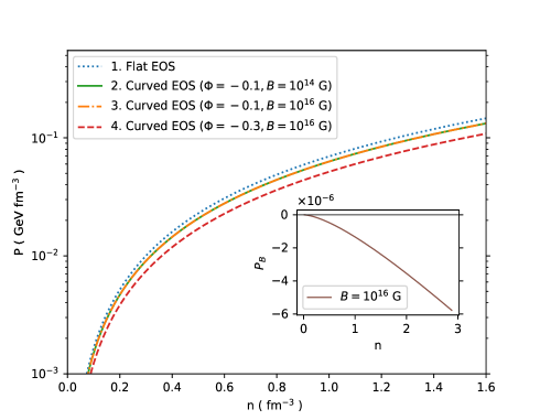
Figure 3: Plot of the pressure $P$ exerted by an ensemble of degenerate protons under an external magnetic field $B$ as a function of number density $n$ for different kinematical values of metric function $\Phi$. The curves $2$ and $3$ with different values of magnetic field $B$ are almost indistinguishable. The change of pressure due to the non-zero magnetic field $B$ is shown in the inset plot using same units as the main plot. It shows that effect of magnetic field on the pressure is rather small compared to the effect of gravitational time-dilation.

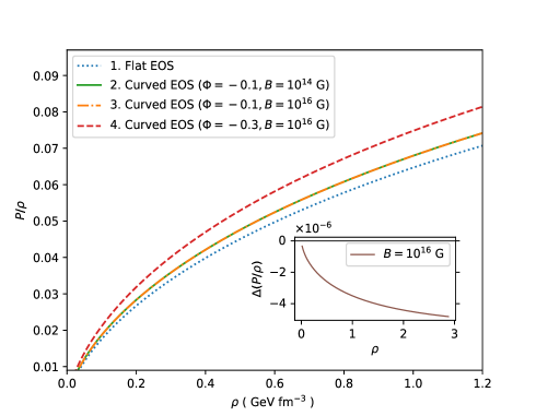
Figure 4: Plot of the ratio $P/\rho$ as a function of the energy density $\rho$ for different values of magnetic field $B$ and metric function $\Phi$. As earlier, the curves $2$ and $3$ with different values of $B$ are nearly indistinguishable. The change of the ratio $P/\rho$ due to the magnetic field i.e. $\Delta(P/\rho)\equiv(P/\rho)_{B}-(P/\rho)_{B=0}$ is shown in the inset plot. As earlier, we note that the effect of gravitational time-dilation on the equation of state is large compared to the effect of an external magnetic field. Nevertheless, due to formation of the Landau levels the effect of an external magnetic field on degenerate protons makes the EOS softer, unlike the case of neutrons.

VI.3 Possible probe for de-confined quarks

We note that for electrically charged fermions, an external magnetic field $B$ leads to $\mathcal{O}(B)$ corrections to the EOS. Further, these modifications are enhanced by the effects of curved spacetime and quantitatively these enhancements are dependent on the specific mass-radius curve of the star. Therefore, in principle one may use the presence of magnetic field as a possible probe for the existence of de-confined quarks which maybe present in the core of a neutron star (for example, see [26, 27, 28, 29, 30]). The quarks are known to be lighter compared to the nucleons. For example, the Up quark has mass, say $m_{q}$, of around $2.2$ MeV and it has electrical charge $e_{q}=2e/3$ which implies its characteristic magnetic field to be $B_{c}=m_{q}^{2}/e_{q}\sim 10^{15}$ Gauss. Therefore, if the core of a neutron star has de-confined quark degrees of freedom and it has magnetic field of around $10^{15}$ Gauss as indicated by observations then the EOS near the core of a neutron star should pick up a substantial corrections due to the magnetic field.

VII Discussions

In summary, in this article we have shown that for an ensemble of electrically neutral degenerate neutrons both magnetic field and gravitational time-dilation leads the EOS to become stiffer. However, for electrically charged fermions the magnetic field makes the EOS to become softer due to formation of the Landau levels. Nevertheless, the changes of EOS due to the gravitational time dilation is relatively stronger than the changes due to the observed strengths of magnetic field. We have shown that in presence of a non-zero magnetic field, a thin layer containing only spin-up neutrons would form at the boundary of a degenerate neutron star. Hence, a neutron star would acquire a non-zero magnetic moment which in turn would lead to an accretion of charged particles surrounding the star. Further, we have argued that a strong magnetic field can act like a possible probe for existence of de-confined quarks in the core of a neutron star where the effects of curved spacetime would enhance the modifications of the EOS.