Limitations on the maximal level of entanglement of two singlet-triplet qubits in GaAs quantum dots

Abstract

We analyze in detail a procedure of entangling of two singlet-triplet ($S$-$T_{0}$) qubits operated in a regime when energy associated with the magnetic field gradient, $\Delta B_{z}$, is an order of magnitude smaller than the exchange energy, $J$, between singlet and triplet states [Shulman M. et al., Science 336, 202 (2012)]. We have studied theoretically a single $S$-$T_{0}$ qubit in free induction decay and spin echo experiments. We have obtained analytical expressions for time dependence of components of its Bloch vector for quasistatical fluctuations of $\Delta B_{z}$ and quasistatical or dynamical $1/f^{\beta}$-type fluctuations of $J$. We have then considered the impact of fluctuations of these parameters on the efficiency of the entangling procedure which uses an Ising-type coupling between two $S$-$T_{0}$ qubits. Particularly, we have obtained an analytical expression for evolution of two qubits affected by $1/f^{\beta}$-type fluctuations of $J$. This expression indicates the maximal level of entanglement that can be generated by performing the entangling procedure. Our results deliver also an evidence that in the above-mentioned experiment $S$-$T_{0}$ qubits were affected by uncorrelated $1/f^{\beta}$ charge noises.

I Introduction

Spin qubits based on gated quantum dots (QDs) [1, 2, 3] can be initialized, coherently controlled, and read out. Qubits based on a spin of a single electron [4] localized in a QD can be controlled with electron-spin resonance techniques [5, 6, 7], while two-qubit gates can be performed with the help of exchange interaction [4, 8, 9], which is controlled electrically [10, 11, 12, 13, 14, 15, 16]. Implementation of single-spin control with ac electric [6, 7, 17] and magnetic [5, 11] fields is nevertheless experimentally challenging, especially in GaAs based QDs, in which interaction with nuclei [18, 19, 20, 21] leads to significant broadening of electron spin resonance lines (this is in contrast to experimental situation in Si-based single-electron QDs [22, 23, 24], for which nuclear noise can be removed by isotopic purification [24, 25]). Research on all-electrical control (possibly without ac fields) is an active field. Such a control is possible for spin qubits based on a few electrons localized in multiple quantum dots [2]. In a double quantum dot (DQD) containing two electrons one can easily initialize and partially control a qubit, whose logical states correspond to singlet $S$ and unpolarized triplet $T_{0}$ formed by the two electrons [10] (note that one can as well use two QDs with larger odd number of electrons per dot [26]), and all-electrical ac control is also possible in a variety of other designs based on two [27], three [28, 29, 30] and four [31] electrons. We focus here on the DQD-based two-electron singlet-triplet ($S$-$T_{0}$) qubit, for which full electrical control over the state of the qubit is possible when the spin splittings of electrons localized in the two dots are distinct. This can be achieved with creation of a gradient of nuclear spin polarization [32, 33] in nuclear spin rich material such as GaAs or with the help of micromagnets creating a gradient of magnetic field [11].

Creation of entanglement [34, 35] of two spin-based qubits is the next necessary step in development of a QD spin qubit platform for quantum information processing. For two single-spin qubits, exchange interaction leads to creation of entangled two-qubit states [11, 36, 15, 12], while in the case of $S$-$T_{0}$ qubits it is the electric dipole-dipole (capacitive) interaction [37] that has been most commonly used for interqubit coupling [38, 39] (although exchange coupling could be used too [40, 41, 42]). Our focus in the present paper is on creation of entanglement and its evolution due to capacitive interqubit interaction, as it was demonstrated experimentally for two $S$-$T_{0}$ qubits in Ref. [39].

Interaction of qubits with their environments that fluctuate in an uncontrolled manner leads to decoherence [43] of their quantum states. In this process, the entanglement, which requires existence of a coherent superposition of at least two product states of the two qubits, is also destroyed [35]. For single electron spins in QDs, the dominant cause of entanglement decay is their hyperfine interaction with the nuclear baths [44, 45]. Decoherence of $S$-$T_{0}$ qubits, on the other hand, can be dominated by the nuclear bath at low singlet-triplet splitting [46], but for large splittings it is mostly caused by charge noise [47, 48, 49], with the nuclear-induced decay [50, 51] possibly playing a role when the fluctuations of $S$-$T_{0}$ splitting are suppressed [52]. Influence of quasistatic charge and nuclear noises on the simplest protocol of generation of entanglement of two capacitively coupled $S$-$T_{0}$ qubits was considered in Ref. [53]. In this paper, we consider a more involved protocol from Ref. [39] under the influence of dynamical charge noise.

In the experiment [39], the two $S$-$T_{0}$ qubits were initialized in a separable state, and subsequently they were evolving in the presence of a finite singlet-triplet splitting $J$. With both qubits having nonzero $J$, dipolar interaction between them leads to the appearance of an Ising-type interaction, which in the decoherence-free case would lead to periodic creation of maximal two-qubit entanglement. In the experiment, only one period of such entanglement oscillation (with entanglement reaching only a fraction of its maximal possible value) is visible. Furthermore, for the entanglement to be nonzero the two qubits have to be subjected to a spin echo refocusing pulse that removes the influence of the slowest environmental fluctuations on their evolution. The strong decoherence is significantly affecting the entanglement generation and evolution. The goal of this paper is to understand processes originated from nuclear polarization fluctuations and charge noise affecting the singlet-triplet splittings which limit the ability to generate entangled two-qubit states for experimental protocol performed in Ref. [39]. The main conclusion of our work is that the spin echo protocol removes most of the influence of the nuclear polarization fluctuations, and the observed decoherence is caused by charge noise. The experimental data from Ref. [39] are consistent with the assumption that each qubit is subjected to $1/f^{\beta}$ charge noise with $\beta\!\lesssim\!1$ (as seen for a single $S$-$T_{0}$ qubit [49]), and the noises affecting the two qubits are independent. We also discuss the qualitative difference in the character of the dominant decoherence process between the cases of small $\beta\!\lesssim\!1$ and large $\beta\!>\!1$ – in the former case the imperfectly echoed-out single-qubit noise has dominant influence, while in the latter case of very low frequency noise the fluctuations of two-qubit coupling are the main reason for imperfect entanglement.

The paper is organized as follows. In Sec. II we give an overview of the physics of a single $S$-$T_{0}$ qubit, and we discuss the influence of fluctuating external magnetic or electric fields on the decoherence of such qubit seen in the free induction decay (FID) as well as spin echo (SE) experiments. In Sec. III we recall a procedure that has been designed for entangling two $S$-$T_{0}$ qubits [39]. We briefly discuss ways of entanglement quantification that have been applied to the system of two qubits in Sec. IV. In Sec. V we then analyze the influence of the above-mentioned factors that lead to decoherence on the efficiency of the procedure of entangling of two $S$-$T_{0}$ qubits. We show here that a dynamically fluctuating electric field affecting qubits’ exchange splittings may limit the maximal level of two-qubit state entanglement by destroying two-qubit entangling gate or simply by dephasing of single qubits. Finally, Sec. VI closes the paper with a discussion of conclusions on the nature of charge noise in the system studied in Ref. [39] that one can draw by comparing the results of our calculations to the observations described there. In the appendices we present explicit expressions that describe the averaged values of $S$-$T_{0}$ qubit components as functions of a duration of free induction decay and spin echo experiments as well as attenuation factors originated from $1/f^{\beta}$ dynamical noise of exchange splittings of the qubits.

II The physics of a Singlet-Triplet qubit

II.1 The Hamiltonian and control over the qubit

In a singlet-triplet qubit, the quantum state is stored in the joint spin state of two electrons in a DQD, with one electron localized in each of the two dots, the left (L) and the right (R) one [37, 10, 33, 49]. The logical states of the qubit are the singlet $|S\rangle~{}~{}=~{}\frac{1}{\sqrt{2}}(\left|\uparrow_{L}\downarrow_{R}\right\rangle-\left|\downarrow_{L}\uparrow_{R}\right\rangle)$ and the spin unpolarized triplet $|T_{0}\rangle~{}=~{}\frac{1}{\sqrt{2}}(\left|\uparrow_{L}\downarrow_{R}\right\rangle+\left|\downarrow_{L}\uparrow_{R}\right\rangle)$. The remaining two states, spin polarized triplets, $\left|\uparrow_{L}\uparrow_{R}\right\rangle$ and $\left|\downarrow_{L}\downarrow_{R}\right\rangle$, are split off by the constant magnetic field applied in the plane of the nanostructure. In the paper, we adopt the convention that the Bloch sphere of $S$-$T_{0}$ qubit is defined in such a way that state $|S\rangle$ ($|T_{0}\rangle$) coincides with north (south) pole of the sphere and the axis connecting these two points is the $z$ axis.

It was demonstrated in Ref. [10] that it is possible to reliably initialize the two electron spins in singlet state $|S\rangle$, perform rotations around $z$ axis of the Bloch sphere, as well as a read-out in a form of projective measurements onto $|S\rangle$. All these operations can be realized utilizing the fast control of the exchange interaction that is achieved by applying proper voltage pulses to the metallic gates on the surface of the sample. The states $|S\rangle$ and $|T_{0}\rangle$ are naturally split by energy $J$ due to the exchange interaction between electrons in the DQD [8, 9]. This energy difference can be influenced by controlling either the energy difference between the ground single-electron states of the two dots (the so-called detuning $\epsilon$) [10, 54], or the height of the inter-dot barrier [4, 14]. According to Ref. [39], the value of $J$ can be varied from much less than $1~{}\mu$eV to a few $\mu$eV on a time scale of a nanosecond. We have then the following time-dependent and externally controlled term in the Hamiltonian of the qubit (in units of $\hbar$):

$$\hat{H}_{J}(t)=J(t)\frac{\hat{\sigma}_{z}}{2}\,\,,$$ (1)

where $\hat{\sigma}_{z}=|S\rangle\langle S|-|T_{0}\rangle\langle T_{0}|$.

Rotations about the $x$ axis of the Bloch sphere (or equivalently, the rotations between $\left|S\right\rangle$ and $\left|T_{0}\right\rangle$ states) present a greater challenge. In Ref. [33] it was realized with the help of an interdot gradient of electron spin splitting $\Delta B_{z}$ caused by difference of nuclear polarizations in the two dots. If the local fields (either nuclear Overhauser fields, or magnetic fields from external magnets) in both dots were identical, $|S\rangle$ and $|T_{0}\rangle$ states would not experience any dynamics, since the phase acquired by spin-down state $\left|\downarrow_{L}\right\rangle$ (spin-up state $\left|\uparrow_{L}\right\rangle$) of the electron in the $L$ dot would be cancelled by the spin-up state $\left|\uparrow_{R}\right\rangle$ (spin down state $\left|\downarrow_{R}\right\rangle$) of the electron in the second dot. The field gradient breaks this symmetry, which can be seen in the following example, where we allow $|S\rangle$ to evolve for time $t$

$$|S\rangle =\frac{1}{\sqrt{2}}\left(\left|\uparrow_{L}\downarrow_{R}\right\rangle-\left|\downarrow_{L}\uparrow_{R}\right\rangle\right)$$

$$\xrightarrow{t}\frac{1}{\sqrt{2}}\left(\left|\uparrow_{L}\downarrow_{R}\right\rangle-\mathrm{e}^{it{\Delta B_{z}}}\left|\downarrow_{L}\uparrow_{R}\right\rangle\right)\,.$$ (2)

We can see that the initial state transforms back-and-forth between singlet and the unpolarized triplet, as the phase factor oscillates between $1$ and $-1$ with frequency set by $\Delta B_{z}$. The field gradient $\Delta B_{z}$ contributes the following term to the qubit’s Hamiltonian:

$$\hat{H}_{\Delta B_{z}}=\Delta B_{z}\frac{\hat{\sigma}_{x}}{2}\,\,,$$ (3)

where $\hat{\sigma}_{x}=\left|S\right\rangle\left\langle T_{0}\right|+\left|T_{0}\right\rangle\left\langle S\right|$.

The difficulty in the realization of precise singlet-to-triplet transitions lies in the fact that the necessary field gradient, in most cases, is generated by the slowly fluctuating Overhauser field established by the nuclear spins of the atoms comprising the sample [55]. Therefore, $\Delta B_{z}$ must be treated as given (in fact, it must be measured beforehand, and the value of $\Delta B_{z}$ varies in different repetitions of the experiment), hence, it would induce an ongoing transition between $\left|S\right\rangle$ and $\left|T_{0}\right\rangle$, which is undesirable in the context of the entangling procedure. Instead, such a procedure requires precise state transformations on demand. For example, if one desires to execute a rotation from $\left|S\right\rangle$ to $\left|T_{0}\right\rangle$ at a given moment $t^{\prime}$ it would be ideal if $\Delta B_{z}$ could be turned on only for an interval $[t^{\prime},t^{\prime}+\pi/\Delta B_{z}]$, so that the phase in Eq. (2) is $\mathrm{e}^{i\Delta B_{z}\cdot(t^{\prime}+\frac{\pi}{\Delta B_{z}}-t^{\prime})}=\mathrm{e}^{i\pi}=-1$. Since there is no practical way to change the value of $\Delta B_{z}$ during a single realization of the procedure, one cannot simply turn off the gradient and stop the transition. Nevertheless, the transition can be effectively blocked by overshadowing $\Delta B_{z}$ with strong enough splitting $J$, which can be controlled with relative ease, and it can be switched on and off at will. In order to realize the idealized scenario such as the one described above, the time scale on which $J$ is manipulated must be the shortest time scale in the problem. In particular, this time scale must be much shorter than the period of rotations around $x$-axis $1/\Delta B_{z}$ as well as the period of $z$-rotations set by the maximal value of singlet-triplet splitting $1/J_{\mathrm{max}}$. Note that pulse-shaping techniques for gate error mitigation were derived for $S$-$T_{0}$ qubits [56, 57, 58], but their implementation has proven to be challenging so far, and we focus here on the simplest control scheme used in experiment on creation of entanglement in Ref. [39]. Let us also note that entanglement of two $S$-$T_{0}$ qubits in the situation in which $\Delta B_{z}$ is always larger than $J$ was generated using a scheme involving ac control of $J$ [59], which is distinct from the one used in Ref. [39] and analyzed here.

II.2 Decoherence of a single $S$-$T_{0}$ qubit

II.2.1 The nature of noisy terms in the Hamiltonian

A qubit evolving with nominally constant $\Delta B_{z}$ and $J$ is undergoing decoherence due to uncontrolled fluctuations of these parameters. When the magnetic field gradient $\Delta B_{z}$ is due to the difference of the $z$ components of nuclear Overhauser fields in the two dots (which is the case on which we focus here), the main mechanism responsible for its fluctuations is the spin diffusion process [55, 60] caused by dipolar interactions between the nuclear spins. Note that we focus here on $J\!\gg\Delta B_{z}$ regime, in which only the large-amplitude classical fluctuations of the Overhauser fields can affect the qubit. This is in contrast to $J\!\ll\!\Delta B_{z}$ case, in which a quantum treatment of nuclear fluctuations is necessary [61, 62, 63]. The large-amplitude fluctuations have a characteristic decorrelation time scale of about one second [55, 60], which is much longer than the time scale of a single run of the experiment, i.e. a single repetition of qubit’s initialization – evolution – measurement cycle. Therefore, $\Delta B_{z}(t)$ can be treated as quasistatic [64, 19, 51], i.e. it is considered as a constant (i.e. time independent) random variable with certain probability distribution $p(\Delta B_{z})$. For a large number of nuclei, this distribution is normal [65], with the average value $\overline{\Delta B_{z}}$ and dispersion (standard deviation) $\sigma_{\Delta B_{z}}=\sqrt{\overline{\Delta B_{z}^{2}}-(\overline{\Delta B_{z}})^{2}}$. Within this approximation, the result of the experiments are interpreted as follows. Given the initial density operator of the qubit, $\hat{\rho}(0)=\hat{\rho}_{\mathrm{ini}}$, its evolution during the experiment run number $n$, is described by the qubit Hamiltonian $\hat{H}_{\mathrm{q}}(t)=\hat{H}_{J}(t)+\hat{H}_{\Delta B_{z}}$ with an unknown, but constant, value of $\Delta B_{z}=\Delta B_{z}^{n}$ drawn from the distribution $p(\Delta B_{z})$,

$$\hat{\rho}(t|\Delta B_{z}^{n}) =\mathrm{e}^{-it(J\hat{\sigma}_{z}+\Delta B_{z}\hat{\sigma}_{x})/2}\hat{\rho}_{\mathrm{ini}}$$

$$\times\mathrm{e}^{it(J\hat{\sigma}_{z}+\Delta B_{z}\hat{\sigma}_{x})/2}\Big{|}_{\Delta B_{z}=\Delta B_{z}^{n}}\,.$$ (4)

The final results are derived from the whole series of $N$ experiment repetitions with the same initial state. Therefore, the expectation values of the measured quantities are calculated with the help of the averaged density operator according to

$$\hat{\rho}_{\mathrm{fin}}(t) =\frac{1}{N}\sum_{n=1}^{N}\hat{\rho}(t|\Delta B_{z}^{n})$$

$$\xrightarrow{N\to\infty}\int_{-\infty}^{\infty}d(\Delta B_{z})p(\Delta B_{z})\hat{\rho}(t|\Delta B_{z})$$

$$=\overline{\hat{\rho}(t|\Delta B_{z})}\,.$$ (5)

On the other hand, the exchange splitting $J(t)$ changes due to fluctuations of local electric fields, i.e. due to charge noise, which is ubiquitous in semiconductor nanostructures. The charge noise typically has its spectral weight concentrated at low frequencies. Contributions of noise at frequencies corresponding to the inverse of typical qubit coherence are typically negligible when considering free evolution of the qubit (hence the noise can be treated then as quasistatic), but they have to be taken into account when modeling the spin echo experiment [49], in which the influence of the lowest-frequency noise is removed, and coherence times are longer. In order to model the experimental data, one has to average the qubit’s evolution over many realizations of the stochastic process $J(t)$. If the noise statistics is assumed to be Gaussian (which is natural for noise consisting of many independent contributions), and if the evolution can be treated in the pure dephasing approximation (i.e. neglecting $\Delta B_{z}\hat{\sigma}_{x}$ term when $\Delta B_{z}\!\ll\!J(t)$), the averaging can be done analytically. In the case of non-Gaussian noise and when keeping the general form of the Hamiltonian, one has to resort to numerical simulations [66, 67].

It was shown [49] that the GaAs/AlGaAs $S$-$T_{0}$ qubit is affected by noise having power spectral density of $1/f^{\beta}$ form with $\beta\!\approx\!0.7$ in the range of frequencies relevant for correct description of spin echo signal. It is unclear if this value of $\beta$ is specific to this material or only to the device used in that experiment.

II.2.2 Decoherence during free evolution of the qubit

We now assume that the initial state of a qubit is $|{-y}\rangle=\frac{1}{\sqrt{2}}(|S\rangle-i|T_{0}\rangle)$. This choice is connected with the entangling procedure used in Ref. [39], in which this single-qubit state is used as the initial one for both qubits. In a free induction decay (FID) experiment, the qubit undergoes evolution without any manipulations between its initialization and the coherence readout at time $\tau$. With fixed values of $J$ and $\Delta B_{z}$, the expectation values of qubit observables $\langle\hat{\sigma}_{i}^{\mathrm{FID}}(\tau)\rangle=\langle{-y}|\hat{\sigma}_{i}(\tau)|{-y}\rangle$ are given by

$$\langle\hat{\sigma}_{x}^{\mathrm{FID}}(\tau)\rangle =\frac{J}{\sqrt{\Delta B_{z}^{2}+J^{2}}}\sin\Big{(}\sqrt{\Delta B_{z}^{2}+J^{2}}\tau\Big{)}\,\,,$$ (6)

$$\langle\hat{\sigma}_{y}^{\mathrm{FID}}(\tau)\rangle =-\cos\Big{(}\sqrt{\Delta B_{z}^{2}+J^{2}}\tau\Big{)}\,\,,$$ (7)

$$\langle\hat{\sigma}_{z}^{\mathrm{FID}}(\tau)\rangle =-\frac{\Delta B_{z}}{\sqrt{\Delta B_{z}^{2}+J^{2}}}\sin\Big{(}\sqrt{\Delta B_{z}^{2}+J^{2}}\tau\Big{)}\,\,.$$ (8)

The qubit evolves under the influence of $J\!\gg\!\Delta B_{z}$, so to the lowest order in $\Delta B_{z}/J$ the initial amplitude of $x$ and $y$ signals is $\approx 1$, while the $z$ signal has amplitude $\approx\!\Delta B_{z}/J$. In the presence of fluctuations of both $J$ and $\Delta B_{z}$ all these signals will average to zero at long times, at which the arguments of the oscillatory functions taken from an appropriate distribution will have relative phases randomly distributed between $0$ and $2\pi$.

We can average the above expressions over $\Delta B_{z}$ and $J$ assuming Gaussian and quasistatic fluctuations of either of these parameters. We focus on the largest observable, $\langle\hat{\sigma}_{y}^{\mathrm{FID}}(\tau)\rangle$, and we approximate $\sqrt{\Delta B_{z}^{2}+J^{2}}\tau\approx J\tau+\Delta B_{z}^{2}\tau/2J$, which is valid for $J\gg\Delta B_{z}$ and for short durations $\tau\ll 8J^{3}/\Delta B_{z}^{4}$. For $J$ noise we get then a simple Gaussian decay:

$$\left\langle\langle\hat{\sigma}_{y}^{\mathrm{FID}}(\tau)\rangle\right\rangle_{J}\approx-\frac{1}{2}\exp\Big{[}-(\tau/T^{*}_{2,J})^{2}\Big{]}\cos(\bar{J}\tau)\,\,,$$ (9)

where $\bar{J}$ is the average value of $J$ and the decay time scale is

$$T^{*}_{2,J}=\frac{\sqrt{2}}{\sigma_{J}}\,\,,$$ (10)

where $\sigma_{J}$ is the standard deviation of $J$.

Averaging over $\Delta B_{z}$ gives

$$\left\langle\langle\hat{\sigma}_{y}^{\mathrm{FID}}(\tau)\rangle\right\rangle_{\Delta B_{z}} \approx-\exp\left(-\frac{\tau^{2}\overline{\Delta B_{z}}^{2}\sigma_{\Delta B_{z}}^{2}}{2\left(J^{2}+(\sigma_{\Delta B_{z}}^{2}\tau)^{2}\right)}\right)$$

$$\times\frac{1}{\big{(}1+(\sigma_{\Delta B_{z}}^{2}\tau/J)^{2}\big{)}^{1/4}}$$

$$\times\cos\Big{(}r(\tau)+s(\tau)\Big{)},$$ (11)

where $r(\tau)=\frac{1}{2}\arctan\left(\sigma_{\Delta B_{z}}^{2}\tau/J\right)$, and $s(\tau)=J\tau\Big{(}\overline{\Delta B_{z}}^{2}+2J^{2}+2(\sigma_{\Delta B_{z}}^{2}\tau)^{2}\Big{)}/\Big{(}2\big{(}J^{2}+(\sigma_{\Delta B_{z}}^{2}\tau)^{2}\big{)}\Big{)}$. The decay envelope is then a product of two factors. The first one dominates the decay when $\overline{\Delta B_{z}}\!\gg\!\sigma_{\Delta B_{z}}$, i.e. in the situation in which a finite $\Delta B_{z}$ is used for coherent control of the qubit. Then at long $\tau$ this factor saturates at $\exp\big{(}-\overline{\Delta B_{z}}^{2}/2\sigma^{2}_{\Delta B_{z}}\big{)}\!\ll\!1$, and the qubit loses most of its coherence at time scale $\tau\!\ll\!J/\sigma^{2}_{\Delta B_{z}}$, at which the factor can be approximated as $\exp\Big{(}-(\tau/T_{2,\Delta B_{z}}^{*})^{2}\Big{)}$, where

$$T^{*}_{2,\Delta B_{z}}\!=\!\frac{\sqrt{2}}{\sigma_{\Delta B_{z}}}\cdot\frac{J}{\overline{\Delta B_{z}}}\,\,.$$ (12)

On the other hand, when $\overline{\Delta B_{z}}\!\ll\!\sigma_{\Delta B_{z}}$, the second factor dominates, and the signal envelope decays in power law fashion $\propto\!\sqrt{\tau_{\Delta B_{z}}/\tau}$, where the characteristic time $\tau_{\Delta B_{z}}\!=\!J/\sigma^{2}_{\Delta B_{z}}$.

It is important to note now that in the regime of $\bar{J}\!\gg\!\overline{\Delta B_{z}}$ and $\overline{\Delta B_{z}}\!\gg\!\sigma_{\Delta B_{z}}$ (that is relevant for experiments of interest in this paper), we typically have $\sigma_{J}\!\gg\!\sigma_{\Delta B_{z}}$. This is due to the observed relation between $J$ and detuning $\epsilon$: $J\!\approx\!J_{0}\exp(\epsilon/\epsilon_{0})$, and the fact that the noise in $J$ comes mostly from fluctuations of $\epsilon$. We have thus $\delta J/J\sim\delta\epsilon/\epsilon_{0}$, so for constant level of detuning noise the standard deviation $\sigma_{J}$ increases with $J$ [49]. It is then a reasonable assumption to neglect the effect of fluctuations of $\Delta B_{z}$ in the calculation of decoherence. Furthermore, for $\bar{J}\!\gg\!\overline{\Delta B_{z}}$ the main effect of $\overline{\Delta B_{z}}\hat{\sigma}_{x}$ term is a slight tilt in $xOz$ plane of the axis about which the qubit’s Bloch vector is precessing. Neglecting this effect, we arrive at the pure dephasing approximation to the qubit’s Hamiltonian:

$$\hat{H}(t)\approx\left(\bar{J}+\delta J(t)\right)\frac{\hat{\sigma}_{z}}{2}\,\,,$$ (13)

where we have now included the time dependence of $J$ noise. The off-diagonal element of the qubit’s density operator is given by

$$\rho_{ST_{0}}(\tau) =\rho_{ST_{0}}(0)\,\mathrm{e}^{-i\bar{J}\tau}$$

$$\times\left\langle\exp\left(-i\int_{0}^{\infty}f_{\mathrm{FID}}(t;\tau)\delta J(t)\mathrm{d}t\right)\right\rangle_{\delta J}\,\,,$$ (14)

where $\langle...\rangle_{\delta J}$ denotes averaging over different realizations of $\delta J(t)$ noise, and $f_{\mathrm{FID}}(t;\tau)\!=\!\theta(t)\theta(\tau-t)$ is the FID time-domain filter function, where $\theta(t)$ is Heaviside step function. The transverse components of the qubit state are given by $\left\langle\langle\hat{\sigma}_{x}^{\mathrm{FID}}(\tau)\rangle\right\rangle\!=\!2\mathrm{Re}\rho_{ST_{0}}(\tau)$ and $\left\langle\langle\hat{\sigma}_{y}^{\mathrm{FID}}(\tau)\rangle\right\rangle\!=\!2\mathrm{Im}\rho_{ST_{0}}(\tau)$. For Gaussian $\delta J(t)$ noise only the second cumulant of the random phase is nonzero [68, 69, 70], and we have a closed formula for coherence:

$$\rho_{ST_{0}}(\tau)=\rho_{ST_{0}}(0)\,\mathrm{e}^{-i\bar{J}\tau}\,\mathrm{e}^{-\chi_{\mathrm{FID}}(\tau)}\,\,,$$ (15)

in which the attenuation factor $\chi_{\mathrm{FID}}$ is defined in the following way

$$\chi_{\mathrm{FID}} =\int_{0}^{\infty}\mathrm{d}t_{1}\int_{0}^{\infty}\mathrm{d}t_{2}f_{\mathrm{FID}}(t_{1})f_{\mathrm{FID}}(t_{2})\left\langle\delta J(t_{1})\delta J(t_{2})\right\rangle_{\delta J}$$

$$=\int_{0}^{\infty}S(\omega)|\tilde{f}_{\mathrm{FID}}(\omega)|^{2}\frac{\mathrm{d}\omega}{\pi}\,\,,$$ (16)

where in the second line we have assumed that the noise is stationary, so that its autocorrelation function is $C(t_{1}-t_{2})\!=\!\left\langle\delta J(t_{1})\delta J(t_{2})\right\rangle_{\delta J}$. The spectral density of the noise is $S(\omega)\!=\!\int_{-\infty}^{\infty}C(t)\mathrm{e}^{i\omega t}\mathrm{d}t$ and the frequency domain filter function [68, 69] is

$$\tilde{f}_{\mathrm{FID}}(\omega) =\int_{-\infty}^{\infty}f_{\mathrm{FID}}(t;\tau)\mathrm{e}^{i\omega t}\mathrm{d}t$$

$$=2\sin^{2}\left(\frac{\omega\tau}{2}\right)\frac{1}{\omega^{2}}\,\,.$$ (17)

In the case of $S(\omega)\!\sim\!\frac{1}{f^{\beta}}$ with $\beta=0.7$, the attenuation factor defined in Eq. (16) depends on $\tau$ as a power function: $\chi_{\mathrm{FID}}\propto\tau^{1.7}$ (see Appendix B for a detailed calculation).

Note that for $\beta\!\geqslant\!1$ the integral in Eq. (16) diverges. However, in a real experimental setting, the total time of data acquisition, $T_{M}$, involving many repetitions of cycles of qubit initialization, evolution for time $\tau$, and measurement, sets the low-frequency cutoff, $\omega_{\mathrm{min}}\!\sim\!1/T_{M}$, for frequencies of noise that actually affect the qubit [70, 49, 25]. Consequently, the lower limit of the integral in Eq. (16) should be $\omega_{\mathrm{min}}>0$ instead of zero, making the attenuation factor finite. In this paper we are setting $\omega_{\mathrm{min}}/2\pi\!=\!1$ mHz, corresponding to $T_{M}$ in a perfectly realistic range of tens of minutes.

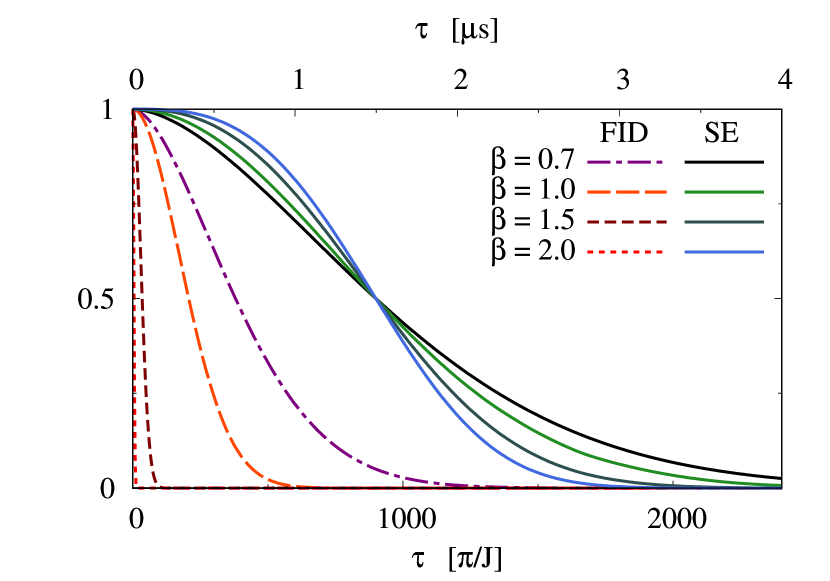
Figure 1: (Color online) FID and SE signals of a single $S$-$T_{0}$ qubit for the case of $1/f^{\beta}$ noise in exchange splitting $J$, with fluctuations in $\Delta B_{z}$ neglected. The power of the noise was chosen to be such that ensures decay of SE signal as observed in the experiment [49] (such a power that leads to half-decay of SE signal in 1.5 $\mu s$ for $J\!\approx\!1$ $\mu$eV). Note that the improvement in coherence time due to echo relative to FID is larger when $\beta$ is larger, i.e. when there is more noise power at the lowest frequencies.

II.2.3 Decoherence in spin echo protocol

The influence of very low frequency noise on qubit dephasing can be removed by employing a spin echo protocol [68], in which a qubit is subjected to a $\pi$ rotation about an axis perpendicular to the axis along which the noise is coupled (here we focus on $\pi$ rotations about the $x$ axis) at time $t=\frac{\tau}{2}$, and the coherence is read out at the final time $t=\tau$.

Within the pure dephasing approximation introduced above, and for perfect short ($\delta$ function like) pulses, the calculation of echoed coherence signal as a function of duration $\tau$ of the echo procedure amounts to replacing the $f_{\mathrm{FID}}(t)$ function in Eq. (14) by the $f_{\mathrm{SE}}(t)$ function which is nonzero for $t\in[0,\tau]$ and changes its value from $1$ to $-1$ at $t=\tau/2$, see e.g. Refs. [68, 70]. The coherence at the final readout time is given by a formula analogous to Eq. (15), only with $\chi_{\mathrm{FID}}(\tau)$ replaced by $\chi_{\mathrm{SE}}(\tau)$ in which $\tilde{f}_{\mathrm{SE}}(\omega)=4\sin^{4}\frac{\omega\tau}{4}/\omega^{2}$ appears. The latter filter function strongly suppresses very low $\omega$ contribution (precisely from $\omega\!\ll\!4\tau$ range) to the attenuation factor $\chi_{\mathrm{SE}}(\tau)$. For quasistatic charge noise we have $S(\omega)\!\approx\!\sigma_{J}\delta(\omega)$, and the echo protocol leads to a complete recovery of the initial coherence.

For $J$ noise with nontrivial spectrum, but with a lot of noise power at low frequencies, the echo decay time is expected to be much longer than the FID decay time, see Fig. 1 for illustration. Recall that our justification for the neglect of quasistatic $\Delta B_{z}$ fluctuations was that in the experimentally relevant parameter regime they lead to much slower FID decay than the $J$ fluctuations. Echo-induced suppression of $J$ noise effects could be suspected of leading to breakdown of that assumption. This is not the case: the echo protocol is also strongly suppressing the effects of quasistatic transverse noise, provided that the effective transverse field $\Delta B_{z}$ is much smaller than the typical longitudinal field. For given values of $J$ and $\Delta B_{z}$ we have

$$\langle\hat{\sigma}_{y}^{\mathrm{SE}}(\tau)\rangle =\langle{-y}|\mathrm{e}^{i\hat{H}\frac{\tau}{2}}(i\hat{\sigma}_{x})\mathrm{e}^{i\hat{H}\frac{\tau}{2}}\hat{\sigma}_{y}$$

$$\times\mathrm{e}^{-i\hat{H}\frac{\tau}{2}}(-i\hat{\sigma}_{x})\mathrm{e}^{-i\hat{H}\frac{\tau}{2}}|{-y}\rangle$$

$$=\frac{1}{\Delta B_{z}^{2}+J^{2}}\Big{(}J^{2}+\Delta B_{z}^{2}\cos\Big{(}\sqrt{\Delta B_{z}^{2}+J^{2}}\tau\Big{)}\Big{)}\,\,.$$ (18)

As before, this expression can be analytically averaged over $\Delta B_{z}$ for short durations $\tau\ll 8J^{3}/\Delta B_{z}^{4}$. The full result is more complicated than Eq. (11) (see Appendix A for full expression), but for $\sigma^{2}_{\Delta B_{z}}\tau/J\!\gg\!(\Delta B_{z}/\sigma_{\Delta B_{z}})^{2}$ one can arrive at

$$\left\langle\langle\hat{\sigma}_{y}^{\mathrm{SE}}(\tau)\rangle\right\rangle_{\Delta B_{z}} \approx\frac{J^{2}}{J^{2}+\overline{\Delta B_{z}}^{2}}$$

$$+\frac{\sigma^{2}_{\Delta B_{z}}}{2\left(J^{2}+\overline{\Delta B_{z}}^{2}\right)}\left(\frac{J}{\sigma^{2}_{\Delta B_{z}}\tau}\right)^{3/2}$$

$$\times\cos\left(J\tau\right)\,\,,$$ (19)

where we see that at long times the only effect of quasistatic transverse noise is decrease of the coherence signal by an amount $\approx(\overline{\Delta B_{z}}/J)^{2}\!\ll\!1$ compared to its initial value.

The echo signal averaged over quasistatic fluctuations of $J$ looks similarly

$$\langle\langle\hat{\sigma}_{y}^{\mathrm{SE}}(\tau)\rangle\rangle_{J} \approx\frac{\bar{J}^{2}+\sigma_{J}^{2}}{\bar{J}^{2}+\Delta B_{z}^{2}}$$

$$+\frac{\Delta B_{z}^{2}}{\bar{J}^{2}+\Delta B_{z}^{2}}\exp\left(-\frac{\sigma_{J}^{2}\tau^{2}}{2}\right)$$

$$\times\cos\left(\bar{J}\tau\right).$$ (20)

For long times, the signal $\langle\langle\sigma_{y}^{\mathrm{SE}}(\tau)\rangle\rangle_{J}$ remains close to its initial value ${(\bar{J}^{2}+\sigma_{J}^{2})}/{(\bar{J}^{2}+\Delta B_{z}^{2})}\approx 1$.

III The procedure for entangling two $S$-$T_{0}$ qubits

Now we proceed with the description of the procedure designed in Ref. [39] aimed to create maximally entangled two-qubit states out of an initial product state. Here, let us focus on an idealized setting in which both $J$ and $\Delta B_{z}$ are piecewise-constant and fully controlled, so that no averaging over their values is performed. Of course, in reality only $J$ is controlled, and it furthermore fluctuates – and the consequences of this will be the main subject of subsequent sections.

Entanglement generation requires some kind of qubit-qubit interaction, and in the case of $S$-$T_{0}$ qubits one utilizes the coupling between electric dipoles induced by state-dependent charge distributions in each DQD [37]. Only if both qubits are in state $\left|S\right\rangle$, and their exchange splittings are finite, the charge distributions are asymmetric (due to mixing of the singlet state relevant here with a singlet state of two electrons localized in a single dot), and hence, each DQD possesses a nonzero electric dipole moment. Therefore, the effective Hamiltonian of this interaction is given by (in units of $\hbar$)

$$\hat{H}_{\mathrm{int}}=\frac{1}{4}J_{12}\left|SS\right\rangle\left\langle SS\right|=\frac{1}{4}J_{12}(\hat{\sigma}_{z}+\hat{\mathds{1}})\otimes(\hat{\sigma}_{z}+\hat{\mathds{1}})\,.$$ (21)

It was established empirically in Ref. [39] that for values of splittings $J_{i}$ used there the strength of the interaction is given by

$$J_{12}=\frac{J_{1}J_{2}}{K}\,\,,$$ (22)

where parameter $K$ is a constant. Thus, the control over the exchange splittings (described in the previous section) simultaneously allows to modify the value of the coupling $J_{12}$. Note that the fact that $J_{12}\propto J_{1}J_{2}$ exposes single-qubit gates to crosstalk when nearby $S$-$T_{0}$ qubits have finite $J_{i}$ splittings, and methods for dealing with this issue have been discussed [71]. Furthermore, configuration interaction calculations have suggested the existence of parameter regions for two capacitively coupled $S$-$T_{0}$ qubits in which the relation between $J_{12}$ and $J_{i}$ is more complicated, leading e.g. to predictions of “sweet spots” at which charge-noise induced fluctuations of $J_{i}$ and/or $J_{12}$ are suppressed [72, 73]. Here we focus on noisy behavior of $J_{i}$ measured in Ref. [49] and the resulting noisy behavior of $J_{12}$ following from Eq. (22).

The procedure consists of the following steps. Before each run the value of the gradients of magnetic field $\Delta B_{z,i}$ in each DQD is established (e.g. by a measurement or even setting the value with a dedicated procedure). Then each $S$-$T_{0}$ qubit is independently initialized in $\left|S\right\rangle$ state, yielding a separable two-qubit state

$$\left|\psi(t=0)\right\rangle=\left|S\right\rangle\otimes\left|S\right\rangle\equiv\left|SS\right\rangle\,.$$ (23)

For each qubit, the exchange splitting is turned off for a time interval corresponding to $\frac{\pi}{2}$ rotation around $x$ axis due to magnetic gradients. Generally $\Delta B_{z,1}\neq\Delta B_{z,2}$ (for concreteness, suppose that $\Delta B_{z,1}\geqslant\Delta B_{z,2}$) so that each splitting has to be kept turned off for different time interval $t_{i}=\frac{\pi}{2\Delta B_{z,i}}$. After time $t_{1}$ one obtains

$$\left|\psi(t_{1})\right\rangle= {}\,\mathrm{e}^{-\frac{i}{2}\frac{\pi}{2}\hat{\sigma}_{x}}\otimes\mathrm{e}^{-\frac{i}{2}\Delta B_{z,2}t_{1}\hat{\sigma}_{x}}\left|SS\right\rangle$$

$$= {}\,\frac{1}{\sqrt{2}}\Big{(}\left|S\right\rangle-i\left|T_{0}\right\rangle\Big{)}\otimes\mathrm{e}^{\frac{i}{2}\frac{\pi}{2}\frac{\Delta B_{z,2}}{\Delta B_{z,1}}\hat{\sigma}_{x}}\left|S\right\rangle\,.$$ (24)

Then, the splitting $J_{1}$ is raised to suppress the rotation of qubit $1$ about $x$ axis, while the rotation of qubit $2$ is being completed in time $\delta t=t_{2}-t_{1}$:

$$\left|\psi(t_{1}+\delta t=t_{2})\right\rangle =\mathrm{e}^{-\frac{i}{2}J_{1}\delta t\hat{\sigma}_{z}}\otimes\mathrm{e}^{-\frac{i}{2}\Delta B_{z,2}\delta t\hat{\sigma}_{x}}\left|\psi(t_{1})\right\rangle$$

$$=\frac{1}{\sqrt{2}}\Big{(}\mathrm{e}^{-i\frac{J_{1}\delta t}{4}}\left|S\right\rangle-i\mathrm{e}^{+i\frac{J_{1}\delta t}{4}}\left|T_{0}\right\rangle\Big{)}$$

$$\otimes\frac{1}{\sqrt{2}}\Big{(}\left|S\right\rangle-i\left|T_{0}\right\rangle\Big{)}\,.$$ (25)

In order to remove the phases imprinted on qubits due to finite $\Delta B_{z,i}$, the spin echo sequences are carried out on each qubit. (Of course, in the more realistic setting in which $J$ fluctuates, the need to remove the influence of the slowest of these fluctuations on the final two-qubit state is a much stronger motivation to employ spin echo.) The SE sequence consists of three steps: the evolution with splitting $J_{i}$ over a chosen time interval, $\pi$ rotation of a state about $x$ axis (i.e. $2t_{i}$ interval when the splitting $J_{i}$ is turned off), which is followed by the evolution for the same time interval. In this case, the durations of SE on each qubit are chosen so that both sequences terminate at the same instant $\tau$. Since $t_{1}\neq t_{2}$ this requirement implies that each SE starts at different time, and they last for unequal durations. Simultaneously during the evolution intervals excluding the periods of evolution corresponding to the $\pi$ rotations both splittings are on and hence the two-qubit coupling $\hat{H}_{\mathrm{int}}$ is on as well, thus allowing for qubits to entangle. Figure 2 showcases the time dependence of splittings $J_{1}$ and $J_{2}$ for the entirety of the entangling procedure. At the end of the procedure, the following state is produced:

$$\left|\tau\right\rangle\equiv|\psi(\tau)\rangle =\frac{1}{2}\mathrm{e}^{-\frac{1}{2}iJ_{12}(\tau-3t_{2})}\left|SS\right\rangle$$

$$+\frac{i}{2}\left|ST_{0}\right\rangle+\frac{i}{2}\left|T_{0}S\right\rangle$$

$$-\frac{1}{2}\mathrm{e}^{-\frac{1}{2}iJ_{12}(\tau-3t_{2})}\left|T_{0}T_{0}\right\rangle\,.$$ (26)

Recall that $t_{2}>t_{1}$ because it was assumed that $\Delta B_{z,1}\geqslant\Delta B_{z,2}$ without loss of generality (if $\Delta B_{z,2}>\Delta B_{z,1}$ simply relabel the qubits to obtain the same result). Note that in the currently considered case of fixed $J$ and $\Delta B_{z}$ the latter drops out from the final state $|\tau\rangle$.

It should be noted that for the discrete set of durations $\tau=\tau_{\mathrm{ent}}^{(a)}=(2a-1)\frac{\pi}{J_{12}}+3t_{2}$, where $a$ is a natural number, the state $|\tau\rangle$ is maximally entangled, specifically, for odd or even $a$ the entangling procedure generates the state

$$|\psi_{\mathrm{o}}\rangle=\frac{i}{2}\left(-|SS\rangle+|ST_{0}\rangle+|T_{0}S\rangle+|T_{0}T_{0}\rangle\right)$$ (27)

or

$$|\psi_{\mathrm{e}}\rangle=\frac{i}{2}\left(|SS\rangle+|ST_{0}\rangle+|T_{0}S\rangle-|T_{0}T_{0}\rangle\right),$$ (28)

respectively. One can easily notice that the entangling procedure realizes a CPHASE gate: $-\mathrm{e}^{-iJ_{12}\frac{\tau-3t_{2}}{2}}|SS\rangle\langle T_{0}T_{0}|-|ST_{0}\rangle\langle T_{0}S|-|T_{0}S\rangle\langle ST_{0}|-\mathrm{e}^{-iJ_{12}\frac{\tau-3t_{2}}{2}}|T_{0}T_{0}\rangle\langle SS|$.

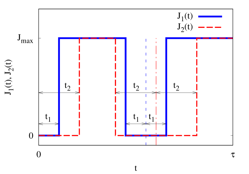
Figure 2: (Color online) The temporal control of the exchange splittings $J_{1}(t),~{}J_{2}(t)$ during execution of the entangling procedure when the magnetic field gradients $\Delta B_{z,1}\neq\Delta B_{z,2}$. Thin vertical blue dashed and red dash-dotted lines are positioned at the middle of the durations of $\pi$ pulses for qubit 1 and 2, respectively.

IV The quantification of two-qubit entanglement

The next step is to quantify the level of entanglement possessed by the two-qubit state $\left|\tau\right\rangle$ produced at the end of the entangling procedure. For two-qubit states described by the density operator $\hat{\rho}$ the most commonly used measure of entanglement is the concurrence [74]. It is defined as

$$C(\hat{\rho})=\mathrm{max}\left\{0,\lambda_{1}-\lambda_{2}-\lambda_{3}-\lambda_{4}\right\}\,,$$ (29)

where $\lambda_{1}\geqslant\lambda_{2}\geqslant\lambda_{3}\geqslant\lambda_{4}$ are the square roots of the eigenvalues of the matrix $\hat{\rho}\hat{\tilde{\rho}}$, where $\hat{\tilde{\rho}}=(\hat{\sigma}_{y}\otimes\hat{\sigma}_{y})\hat{\rho}^{*}(\hat{\sigma}_{y}\otimes\hat{\sigma}_{y})$. Here ${\hat{\rho}}^{*}$ denotes the operation of complex conjugation of each element of $\hat{\rho}$. The concurrence ranges from $C=0$ for separable states to $C=1$ for maximally entangled states. The concurrence of a pure state is given by a simple formula: $C=|\langle\psi|\hat{\sigma}_{y}\otimes\hat{\sigma}_{y}|\psi^{*}\rangle|$, where $|\psi^{*}\rangle$ is a complex conjugation of $|\psi\rangle$.

For the family of output states $\hat{\rho}(\tau)=|\tau\rangle\langle\tau|$ the concurrence is given by

$$C\left(\hat{\rho}(\tau)\right)=\left|\sin\left[\frac{1}{2}J_{12}(\tau-3t_{2})\right]\right|\,.$$ (30)

One can make use of an alternative strategy to check to what degree the resulting state is entangled: high level (greater than 1/2) of fidelity calculated between the actual state $|\tau\rangle$ and the expected entangled state $|\psi_{\mathrm{o}}\rangle$ or $|\psi_{\mathrm{e}}\rangle$, defined as $F(|\tau\rangle,|\psi_{\mathrm{o}}\rangle)=|\langle\tau|\psi_{\mathrm{o}}\rangle|^{2}$, confirms the entanglement [39]. In general, for mixed states, fidelity is defined as $F(\hat{\rho}(\tau),\hat{\rho}_{\mathrm{o}})=\mathrm{Tr}\{\hat{\rho}(\tau)\hat{\rho}_{\mathrm{o}}\}$. If one of the states is pure, as we will be having below, fidelity is given by $F(\hat{\rho}(\tau),|\psi_{\mathrm{o}}\rangle)=\langle\psi_{\mathrm{o}}|\hat{\rho}(\tau)|\psi_{\mathrm{o}}\rangle$.

In Fig. 3 we show the results of numerical calculation of concurrence of the final two-qubit state as a function of procedure duration $\tau$ in a model less idealized than in the previous section. While we are still assuming that $J_{i}$ and $\Delta B_{z,i}$ do not experience any fluctuations, we now keep $\Delta B_{z,i}$ fixed during the evolution (as it is the case in experiment), so that the evolution with finite $J_{i}$ does not amount to phase evolution in the computational basis of $S/T_{0}$ states of two qubits, thus necessitating numerical evaluation of the entanglement measure.

Although the impact of always-on $\Delta B_{z,i}$ terms amounts to a small drop of level of entanglement of the resulting state compared to that from the idealized scenario described in the previous section (see Fig. 3), it reveals also another delicate effect: level of entanglement of the resulting state $|\tau\rangle$ starts to oscillate with frequency of precession of single qubit states $\omega_{i}=\sqrt{\Delta B_{z,i}^{2}+J_{i}^{2}}$ due to the fact that in such conditions the qubits’ states rotate around the axis which does not coincide with $z$ axis exactly, but it is tilted in $xz$ plane because of presence $\Delta B_{z}$. Characteristically, the oscillations of entanglement of the state $\hat{\rho}(\tau)$ gradually increase their amplitude with increasing durations for $0<\tau\lesssim 2\frac{\pi}{J_{12}}$ and reach their maximum amplitude at $\tau\approx 2\frac{\pi}{J_{12}}$. Then the amplitude of oscillations decreases for $2\frac{\pi}{J_{12}}\lesssim\tau\lesssim 4\frac{\pi}{J_{12}}$. The observed pattern of fast oscillation of two-qubit entanglement is periodic in duration $\tau$ of the entangling procedure with a period of about $4\frac{\pi}{J_{12}}$. Such a pattern of oscillation amplitude $\tau$-dependence is a consequence of the entangling procedure design: at $\tau=2\frac{\pi}{J_{12}}$ the ideal resulting state $|\tau\rangle=-\frac{1}{2}\left(|S\rangle-i|T_{0}\rangle\right)^{\otimes 2}$ is unentangled due to a very specific combination of phases generated before and after the $\pi$ rotations of qubits’ states. The two-qubit state that is produced in the middle of the idealized realization of the entangling procedure (just before the step of $\pi$ rotations) is fully entangled. However, when the axes around which qubit states precess are tilted from $z$ direction , the initial superposition states of qubits do not rotate in the equatorial plane (as intended) but in a slightly tilted plane. After the $\pi$ rotation around $x$ axes those states land on the plane which is tilted off from the equatorial plane in the opposite direction , and subsequently the phases which qubits’ states acquire during the second half of the procedure are no longer in a perfect correspondence to the previously obtained phases and now they do not counterbalance each other, so the final two-qubit state manifests unexpected entanglement. One can also notice that in the presence of constant $\Delta B_{z,i}$ the period of slow entanglement oscillations is slightly longer compared to the idealized case (see Fig. 3). This fact cannot be illustrated with the help of Bloch sphere as it originates from a two-qubit interaction, but it is evident from the numerical diagonalization of the full two-qubit Hamiltonian: when $\Delta B_{z,i}$ are present, the rate of acquisition of the desired two-qubit phase is slower than that of the ideal case (CPHASE gate is rotated from the basis of $\{|SS\rangle,~{}|ST_{0}\rangle,~{}|T_{0}S\rangle,~{}|T_{0}T_{0}\rangle\}$ to the basis of eigenvectors of the full Hamiltonian, and as a result the rate of two-qubit phase acquisition becomes lower).

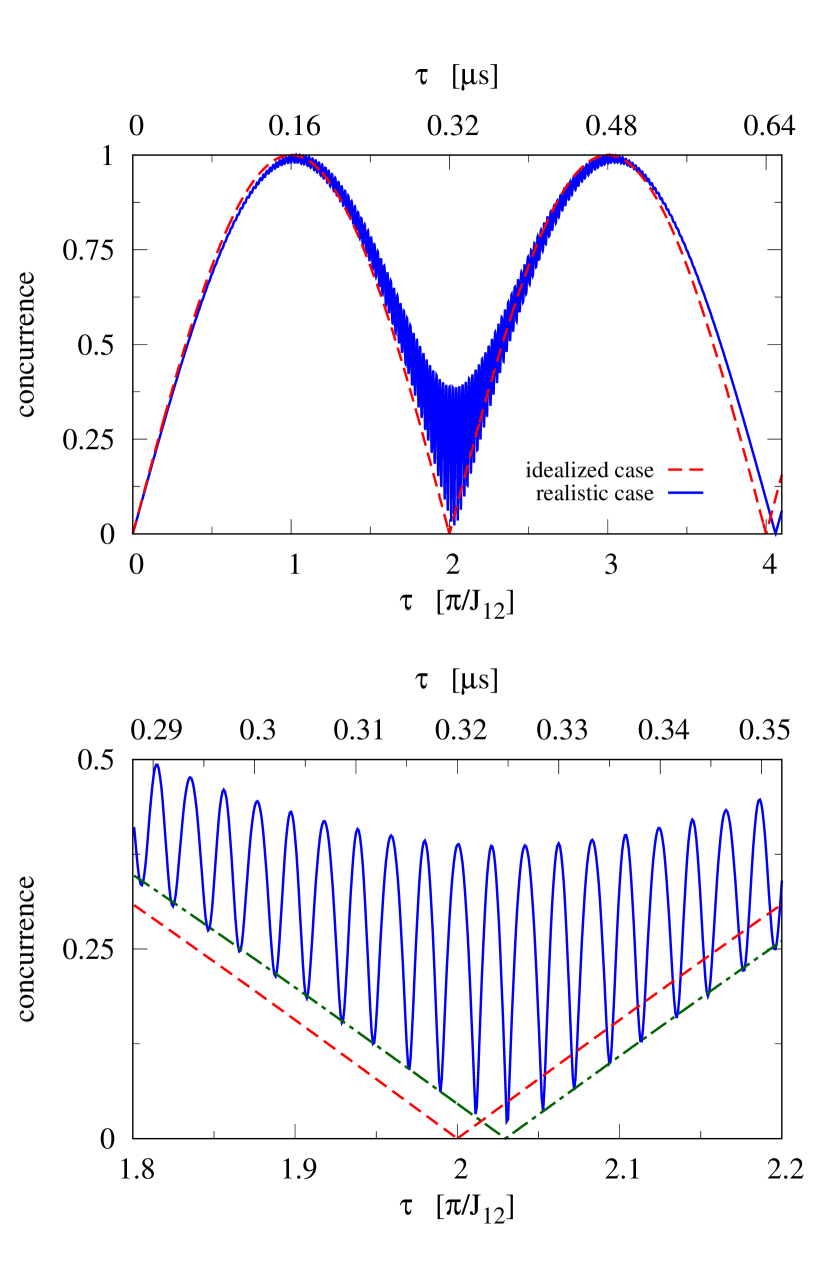
Figure 3: (Color online) Top panel: Concurrence of the two-qubit state generated in the idealized realization of the entangling procedure described in Sec. III ($\Delta B_{z,i}$ are on during the qubit rotations only, the rotations assumed to be perfect) plotted as red dashed line, and the same for a more realistic procedure considered in Sec. IV ($\Delta B_{z,i}$ are always on, albeit none of the parameters of the Hamiltonian are fluctuating) plotted as a solid blue line. The parameters are close to those from the experiment [39]: $J_{1}\!=\!J_{2}\!=\!1.2$ $\mu$eV (with corresponding frequency $J_{i}/h\!=\!300$ MHz), $J_{12}\!=\!1.29\cdot 10^{-2}$ $\mu$eV, $\Delta B_{z,1}\!=\!\Delta B_{z,2}\!=0.12$ $\mu$eV. Bottom panel: zoomed in region of the top panel in the vicinity of $\tau\approx 2\frac{\pi}{J_{12}}$, red dotted line is the concurrence obtained in the idealized case, blue solid line is the concurrence obtained in a more realistic case with constant parameters $J_{i},~{}J_{12}$, $\Delta B_{z,i}$, and green dash-dotted line is the concurrence obtained in the idealized case but with value of $J_{12}$ from the latter case.

V Entangling procedure in the presence of decoherence

In the experiment [39] it turned out that the two-qubit states obtained as outcome of the procedure were indeed entangled but only for short durations $\tau$ of the procedure. Furthermore, the maximal level of entanglement of the generated states was decreased compared to that of the expected ones. We consider below possible factors that preclude one from obtaining the maximally entangled two-qubit states.

V.1 Influence of fluctuations of magnetic field gradients on efficiency of the entangling procedure

The magnetic field gradients between the QDs, which are the sources of finite $\Delta B_{z,i}$ (with $i=1$, $2$), are often produced by the polarized in an appropriate way nuclear spins of the atoms from which the sample is built [33, 39]. The spin bath is dynamically polarized before each iteration of the experiment of entangling of qubits. Due to the slowness of the intrinsic dynamics of the nuclear spin bath, one does not expect any fluctuation on the time scale of a single run of the experiment ($\sim 1~{}\mu\mathrm{s}$). However, possible variations of the values of $\Delta B_{z,i}$ from one run of the experiment to another is the factor which can preclude from obtaining the maximally entangled states. This effect is mainly caused by imprecise rotations of qubits’ states around $x$ axis, which are performed just after the initializations of the qubits in $|SS\rangle$ state ($\frac{\pi}{2}$ rotations) and in the middle of the entangling procedure ($\pi$ rotations). Such systematical errors lead to forming unequal superposition states of $|S\rangle$ and $|T_{0}\rangle$. The influence of quasistatic fluctuations of $\Delta B_{z,i}$ on the efficiency of the entangling procedure results in a decrease of the overall efficiency independently of $\tau$, i.e. the fluctuating quasistatically $\Delta B_{z,i}$ influences in a similar way the outcomes for all duration $\tau$ of the entangling procedure.

This effect can be easily seen when one considers the idealized realization of the procedure: for simplicity, let us assume that only the first rotation was not exactly $\frac{\pi}{2}$ around $x$ axis (errors of rotations $\hat{R}_{x}(\frac{\pi}{2})$ and $\hat{R}_{x}(\pi)$ will accumulate – there is no possibility that the next rotation cancels the error of the previous one). In such a case, the procedure will produce the state $|\tau(\theta_{1},\theta_{2})\rangle=|SS\rangle(-i)\sin\frac{\theta_{1}}{2}\sin\frac{\theta_{2}}{2}\exp(-i\frac{\tau}{2}J_{12})+|ST_{0}\rangle(-i)\sin\frac{\theta_{1}}{2}\cos\frac{\theta_{2}}{2}+|T_{0}S\rangle(-i)\cos\frac{\theta_{1}}{2}\sin\frac{\theta_{2}}{2}+|T_{0}T_{0}\rangle\cos\frac{\theta_{1}}{2}\cos\frac{\theta_{2}}{2}\exp(-i\frac{\tau}{2})$, where $\theta_{i}$ is the actual angle of rotation of the state of $i$th qubit around $x$ axis. This state $|\tau(\theta_{1},\theta_{2})\rangle$ is maximally entangled when superpositions of $|S\rangle$ and $|T_{0}\rangle$, created in each qubit from the separable two-qubit state $|SS\rangle$ after $\hat{R}_{x}(\frac{\pi}{2})$ rotation, are equal (i.e. all components have the same amplitudes): at $\tau=\pi/J_{12}$ the state $|\tau(\theta_{1},\theta_{2})\rangle$ should become $|\psi_{\mathrm{o}}\rangle$, which is maximally entangled, so one can estimate entanglement of $|\tau(\theta_{1},\theta_{2})\rangle$ by calculating fidelity $F(|\tau(\theta_{1},\theta_{2})\rangle,|\psi_{\mathrm{o}}\rangle)=|\langle\tau(\theta_{1},\theta_{2})|\psi_{\mathrm{o}}\rangle|^{2}=\frac{1}{4}|\sin\frac{\theta_{1}}{2}\sin\frac{\theta_{2}}{2}+\sin\frac{\theta_{1}}{2}\cos\frac{\theta_{2}}{2}+\cos\frac{\theta_{1}}{2}\sin\frac{\theta_{2}}{2}+\cos\frac{\theta_{1}}{2}\cos\frac{\theta_{2}}{2}|^{2}$, which has its maximum $F=1$ when $\theta_{1}=\theta_{2}=\frac{\pi}{2}$. Any deviation of $\theta_{1},\theta_{2}\in[0,\pi]$ will reduce the degree of entanglement of the state $|\tau(\theta_{1},\theta_{2})\rangle$. On the other hand, having a pure state $|\tau(\theta_{1},\theta_{2})\rangle$ it is possible to calculate analytically its concurrence $C(|\tau(\theta_{1},\theta_{2})\rangle)=|\langle\tau(\theta_{1},\theta_{2})|\hat{\sigma}_{y}\otimes\hat{\sigma}_{y}|\tau^{*}(\theta_{1},\theta_{2})\rangle|=4\sin\frac{\theta_{1}}{2}\cos\frac{\theta_{1}}{2}\sin\frac{\theta_{2}}{2}\cos\frac{\theta_{2}}{2}\sin(\frac{\tau}{2}J_{12})$, which, when $\tau=\pi/J_{12}$, varies from $C=1$ for $\theta_{1}=\theta_{2}=\frac{\pi}{2}$ to $C=0$ when $\theta_{1},\theta_{2}\rightarrow 0\mathrm{~{}or~{}}\pi$. Hence, the impact of quasistatical fluctuations of magnetic field gradients $\Delta B_{z,i}$ amounts to a loss of the maximal level of produced entanglement (see Fig. 4). This effect is independent of the duration $\tau$ of the procedure and does not lead to a complete inability to yield some entaglement when fluctuations of $\Delta B_{z,i}$ are moderate or small. Another important observation which comes from Fig. 4 is that the presence of quasistatically fluctuating magnetic gradients $\Delta B_{z,i}$ during the entire entangling procedure, does not degrade the efficiency of the procedure by a significant amount while rotations of qubit states around $x$ axis are accurate (cf. line c, which is very close to line b, with line d in Fig. 4).

Consequently, in the rest of the paper, where we will focus on influence of fluctuations of $J_{i}$ that will lead to complete decay of entanglement, we will neglect all the above-discussed effects of quasistatic fluctuations of $\Delta B_{z,i}$ and rotation errors caused by $\Delta B_{z,i}$ being finite, albeit small in comparison to $J_{i}$.

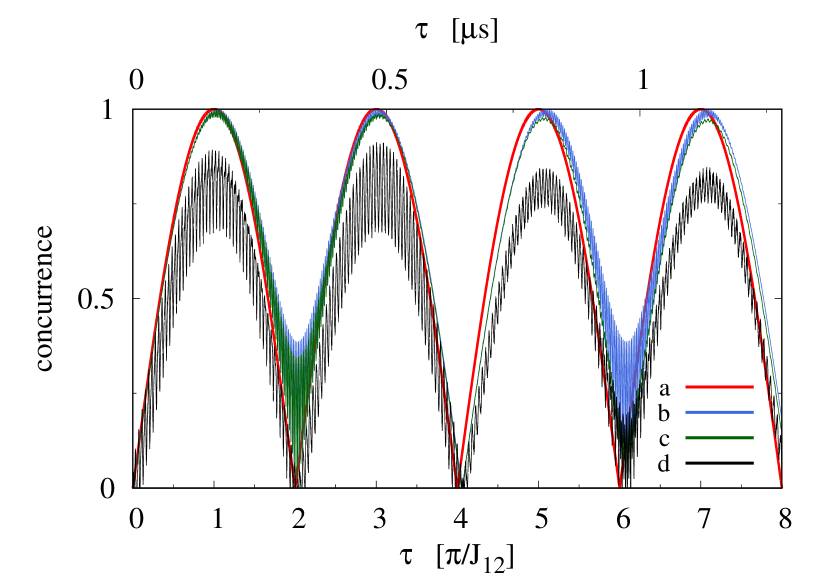
Figure 4: (Color online) Concurrence of the two-qubit state $\hat{\rho}(\tau)$ obtained in (a) idealized realization of entangling procedure (the same as red dashed line in Fig. 3), (b) entangling procedure with always-on constant $\Delta B_{z,i}$ (the same as blue solid line in Fig. 3), (c) entangling procedure in which magnetic field gradients $\Delta B_{z,i}$ are constant during a single run of entangling procedure, but fluctuate quasistatically from one run to another (average over 10,000 realizations, $\Delta B_{z,i}\sim\mathcal{N}(\overline{\Delta B_{z,i}},\,\sigma_{\Delta B_{z,i}})$, $\sigma_{\Delta B_{z,i}}=15\%\,\overline{\Delta B_{z,i}}$), here rotations around $x$ axis artificially kept perfect (i.e. precisely $\frac{\pi}{2}$ at the beginning and $\pi$ in the middle of the procedure), (d) the same as (c) but with imprecise rotations around $x$ axis which arise as a result of mismatch of the rotation time and the actual value of $\Delta B_{z,i}$. All results are obtained under the assumption that $S$-$T_{0}$ splittings $J_{i}$ do not fluctuate and are switched on when needed (as shown in Fig. 2). Values of parameters are the same as in Fig. 3.

V.2 Influence of fluctuations of exchange splittings on efficiency of the entangling procedure

V.2.1 Quasistatic fluctuations of exchange splittings

To begin with, we consider the influence of quasistatic fluctuations of exchange splittings $J_{i}$ on the entanglement generation. The influence of quasistatically fluctuating exchange splittings $J_{1},~{}J_{2}$ can be estimated by disregarding off-diagonal terms of the Hamiltonian (but the qubit rotations involved in the entangling procedure are assumed to be perfect) and performing the averaging of the density operator Eq. (31) over the distribution of $J_{1},~{}J_{2}$. We assume that $J_{1},~{}J_{2}$ fluctuate according to normal distribution with mean values $\bar{J}_{1},~{}\bar{J}_{2}$ and standard deviations $\sigma_{J_{1}},~{}\sigma_{J_{2}}$, respectively.

The idealized entangling procedure generates states which are described by the following density operator:

$$\hat{\rho}(\tau) =|\psi(\tau)\rangle\langle\psi(\tau)|$$

$$=\frac{1}{4}\begin{pmatrix}1&-i\phi(\tau)&-i\phi(\tau)&-1\\ i\phi^{*}(\tau)&1&1&-i\phi^{*}(\tau)\\ i\phi^{*}(\tau)&1&1&-i\phi^{*}(\tau)\\ -1&i\phi(\tau)&i\phi(\tau)&1\end{pmatrix},$$ (31)

where $\phi(\tau)=\exp\left(-i\frac{\tau}{2}J_{12}\right)$. After averaging over quasistatic fluctuations of $J_{1},~{}J_{2}$ we obtain the density operator

$$\langle\hat{\rho}(\tau)\rangle=\frac{1}{4}\begin{pmatrix}1&-i\langle\phi(\tau)\rangle&-i\langle\phi(\tau)\rangle&-1\\ i\langle\phi^{*}(\tau)\rangle&1&1&-i\langle\phi^{*}(\tau)\rangle\\ i\langle\phi^{*}(\tau)\rangle&1&1&-i\langle\phi^{*}(\tau)\rangle\\ -1&i\langle\phi(\tau)\rangle&i\langle\phi(\tau)\rangle&1\end{pmatrix},$$ (32)

where

$$\langle\phi(\tau)\rangle =\frac{2K}{\sqrt{4K^{2}+\sigma_{J_{1}}^{2}\sigma_{J_{2}}^{2}\tau^{2}}}\exp\left(-i\frac{4\bar{J}_{1}\bar{J}_{2}K\tau}{8K^{2}+2\sigma_{J_{1}}^{2}\sigma_{J_{2}}^{2}\tau^{2}}\right)$$

$$\times\exp\left(-\frac{(\bar{J}_{1}^{2}\sigma_{J_{2}}^{2}+\bar{J}_{2}^{2}\sigma_{J_{1}}^{2})\tau^{2}}{8K^{2}+2\sigma_{J_{1}}^{2}\sigma_{J_{2}}^{2}\tau^{2}}\right),$$ (33)

where constant $K~{}=~{}{\bar{J}_{1}\bar{J}_{2}}/{\bar{J}_{12}}$, and $\bar{J}_{12}=\frac{\pi}{\tau_{\mathrm{ent}}}$. In the experiment [39] the values of parameters were as follows: $\bar{J}_{1}\!=\!1.16$ $\mu$eV, $\bar{J}_{2}\!=\!1.32$ $\mu$eV, $\bar{J}_{12}\!=\!1.29\cdot 10^{-2}$ $\mu$eV, $\overline{\Delta B_{z,1}}\!=\!\overline{\Delta B_{z,2}}\!=0.12$ $\mu$eV (so $t_{2}=0$ in the Eq. (30)). Note that we are using $J_{12}$ twice larger than the value reported in Ref. [39]. However, with this value we obtain the period of oscillations of concurrence in agreement with experimental data, i.e. the first maximum of entanglement occurs at $\tau\!=\!\pi/J_{12}\!\approx 160$ ns.

Entanglement of Eq. (32) as a function of duration $\tau$ is shown in the top panel of Fig. 5 for $J_{i}$ drawn from normal distribution with standard deviations $\sigma_{i}=15\%\bar{J}_{i}$. Due to quasistatic fluctuations of $J_{i}$ the overall efficiency of the entangling procedure decreases with increase of its duration $\tau$. Although the direct impact of the quasistatic fluctuations of $J_{1}$, $J_{2}$ on the resulting two-qubit state is completely removed by utilizing simultaneous Hahn echo sequence on each qubit, the entangling interaction between qubits, which is determined by two-qubit interaction energy $J_{12}\propto J_{1}J_{2}$, remains sensitive to the fluctuations, and this causes decay of the entangling procedure efficiency with increasing duration $\tau$.

V.2.2 Dynamical fluctuations of exchange splittings

In the experiment [39] the procedure of entangling two $S$-$T_{0}$ qubits was based on the SE procedure. While the SE perfectly cancels the impact of quasistatic single-qubit noises on the end state, in the case of dynamical fluctuations it helps to refocus the state of the qubits only partially. Moreover, the two-qubit interaction part of the evolution operator that describes the entangling procedure (which is responsible for the entanglement generation) is not affected by the SE procedure, and consequently it is susceptible to noisy electric fields (leading to noise in $J_{i}$ and $J_{12}$) in the same way as in FID experiment. As a result, the overall efficiency of the entangling procedure decays with increasing its duration $\tau$.

In order to estimate analytically the influence of dynamical fluctuations of exchange splittings, we approximate the Hamiltonian of the system by its diagonal neglecting the off-diagonal terms associated with magnetic field gradients $\Delta B_{z,i}$, which were an order of magnitude smaller than exchange splittings $J_{i}$ in the experiment [39]:

$$\hat{H}_{\mathrm{2q}}\approx\hat{H}_{\mathrm{2q}}^{\mathrm{diag}} =\frac{1}{2}\Big{(}J_{1}(t)\hat{\sigma}_{z}\otimes\mathds{1}+J_{2}(t)\mathds{1}\otimes\hat{\sigma}_{z}$$

$$+\frac{1}{2}J_{12}(t)(\hat{\sigma}_{z}+\mathds{1})\otimes(\hat{\sigma}_{z}+\mathds{1})\Big{)}.$$ (34)

Assuming perfect rotations of qubits’ states, averaged density operator elements of the resulting two-qubit state after performing the entangling procedure are

$$\left\langle\rho_{ab,cd}(\tau)\right\rangle=\left\langle\langle ab|\hat{\rho}(\tau)|cd\rangle\right\rangle$$

$$=\langle\langle ab|\hat{U}_{\mathrm{SE}}(\tau)\hat{\rho}^{\mathrm{initial}}\hat{U}_{\mathrm{SE}}^{\dagger}(\tau)|cd\rangle\rangle$$

$$=\langle\langle ab|\hat{U}_{\mathrm{FID}}\Big{(}\frac{\tau}{2},\tau\Big{)}\Big{(}(-i\sigma_{x})\otimes(-i\sigma_{x})\Big{)}\hat{U}_{\mathrm{FID}}\Big{(}0,\frac{\tau}{2}\Big{)}$$

$$\times\sum_{kl,mn}\rho_{kl,mn}^{\mathrm{initial}}|kl\rangle\langle mn|$$

$$\times\hat{U}_{\mathrm{FID}}^{\dagger}\Big{(}0,\frac{\tau}{2}\Big{)}\Big{(}(i\sigma_{x})\otimes(i\sigma_{x})\Big{)}\hat{U}_{\mathrm{FID}}^{\dagger}\Big{(}\frac{\tau}{2},\tau\Big{)}|cd\rangle\rangle,$$ (35)

where evolution operator $\hat{U}_{\mathrm{FID}}(t_{1},t_{2})=\exp\left({-i\int_{t_{1}}^{t_{2}}\hat{H}_{\mathrm{2q}}(t)\mathrm{d}t}\right)\approx\exp\left({-i\int_{t_{1}}^{t_{2}}\hat{H}_{\mathrm{2q}}^{\mathrm{diag}}(t)\mathrm{d}t}\right)$.

Analyzing the two-qubit system, we consider two distinct possibilities of dynamical fluctuations: splitting energies $J_{1}$, $J_{2}$ could fluctuate independently, i.e. $J_{i}(t)=\bar{J}_{i}+\delta J_{i}(t)$, or their fluctuations may have a common source $J_{i}(t)=\bar{J}_{i}+s_{i}\delta J(t)$, where $s_{i}\in[0,1]$ is a coupling of $i$th qubit to the noise. Note that correlations of low-frequency charge noises affecting two quantum dots separated by $\sim\!100$ nm distance have been observed in experiments [77, 78]. Correspondingly, the two-qubit coupling in the former case reads

$$J_{12}(t) =\frac{J_{1}(t)J_{2}(t)}{K}=\frac{1}{K}\left[\bar{J}_{1}+\delta J_{1}(t)\right]\left[\bar{J}_{2}+\delta J_{2}(t)\right]$$

$$\approx\frac{1}{K}\left[\bar{J}_{1}\bar{J}_{2}+\bar{J}_{2}\delta J_{1}(t)+\bar{J}_{1}\delta J_{2}(t)\right]\,\,,$$ (36)

and in the latter case

$$J_{12}(t) =\frac{J_{1}(t)J_{2}(t)}{K}=\frac{1}{K}\left[\bar{J}_{1}+s_{1}\delta J(t)\right]\left[\bar{J}_{2}+s_{2}\delta J(t)\right]$$

$$\approx\frac{1}{K}\left[\bar{J}_{1}\bar{J}_{2}+\left(s_{1}\bar{J}_{1}+s_{2}\bar{J}_{2}\right)\delta J(t)\right]\,\,.$$ (37)

Note that we neglect here the quadratic in noises terms $\propto\delta J_{1}(t)\delta J_{2}(t)$ and $\propto(\delta J(t))^{2}$ .

For the case of independent (completely uncorrelated) charge noises that affect $J_{1}(t)$ and $J_{2}(t)$, the average density operator elements of the generated state are

$$\langle\rho_{ab,cd}(\tau)\rangle=\langle\langle ab|\hat{\rho}(\tau)|cd\rangle\rangle$$

$$=\rho_{-a-b,-c-d}^{\mathrm{initial}}\mathrm{e}^{-i\frac{\bar{J}_{1}\bar{J}_{2}}{4K}(ab-cd)\tau}$$

$$\times\left\langle\exp\Big{[}-\frac{i}{2}\Big{(}\frac{\bar{J}_{2}}{2K}(ab-cd)\int_{0}^{\tau}\mathrm{d}t\,\delta J_{1}(t)f_{\mathrm{FID}}(t)\right.$$

$$\left.+\big{(}c-a+\frac{\bar{J}_{2}}{2K}(c+d-a-b)\big{)}\int_{0}^{\tau}\mathrm{d}t\,\delta J_{1}(t)f_{\mathrm{SE}}(t)\Big{)}\Big{]}\right\rangle$$

$$\times\left\langle\exp\Big{[}-\frac{i}{2}\Big{(}\frac{\bar{J}_{1}}{2K}(ab-cd)\int_{0}^{\tau}\mathrm{d}t\,\delta J_{2}(t)f_{\mathrm{FID}}(t)\right.$$

$$\left.+\big{(}d-b+\frac{\bar{J}_{1}}{2K}(c+d-a-b)\big{)}\int_{0}^{\tau}\mathrm{d}t\,\delta J_{2}(t)f_{\mathrm{SE}}(t)\Big{)}\Big{]}\right\rangle$$ (38)

$$=\rho_{-a-b,-c-d}^{\mathrm{initial}}\mathrm{e}^{-i\frac{\bar{J}_{1}\bar{J}_{2}}{4K}(ab-cd)\tau}$$

$$\times\exp\Big{[}-\frac{1}{2}\Big{\{}\Big{(}\frac{\bar{J}_{2}}{4K}(ab-cd)\Big{)}^{2}\chi_{\mathrm{FID},J_{1}}(\tau)$$

$$+\Big{(}\frac{1}{2}\big{(}c-a+\frac{\bar{J}_{2}}{2K}(c+d-a-b)\big{)}\Big{)}^{2}\chi_{\mathrm{SE},J_{1}}(\tau)\Big{\}}\Big{]}$$

$$\times\exp\Big{[}-\frac{1}{2}\Big{\{}\Big{(}\frac{\bar{J}_{1}}{4K}(ab-cd)\Big{)}^{2}\chi_{\mathrm{FID},J_{2}}(\tau)$$

$$+\Big{(}\frac{1}{2}\big{(}d-b+\frac{\bar{J}_{1}}{2K}(c+d-a-b)\big{)}\Big{)}^{2}\chi_{\mathrm{SE},J_{2}}(\tau)\Big{\}}\Big{]},$$ (39)

where $a,\,b,\,c,\,d\,\in\,\{1,-1\}$ (these parameters code the basis $\{|SS\rangle,|ST_{0}\rangle,|T_{0}S\rangle,|T_{0}T_{0}\rangle\}$ as $\{{11},{1-\!1},{-11},{-1-\!1}\}$ in indices of density operator elements), and $\chi_{\mathrm{FID},J_{i}}(\tau),~{}\chi_{\mathrm{SE},J_{i}}{(\tau)}$ are the attenuation factors that describe the influence of dynamical noise of $J_{i}(t)$ in the case of FID (with constant time domain filter function $f_{\mathrm{FID}}(t)$) or SE (with time domain filter function with a single sign inversion $f_{\mathrm{SE}}(t)$). For noise spectrum of the form $S(\omega)\!=\!A/\omega^{\beta}$ they are given by

$$\chi_{\mathrm{FID}}(\tau) =\frac{4A}{\pi}\int_{0}^{\infty}\frac{\mathrm{d}\omega}{\omega^{2+\beta}}\sin^{2}\frac{\omega\tau}{2}\,\,,$$ (40)

$$\chi_{\mathrm{SE}}(\tau) =\frac{16A}{\pi}\int_{0}^{\infty}\frac{\mathrm{d}\omega}{\omega^{2+\beta}}\sin^{4}\frac{\omega\tau}{4}\,\,,$$ (41)

see Appendix B for the details of derivation and simple analytical approximations in considered here cases of $\beta\!=\!0.7$ and $2$.

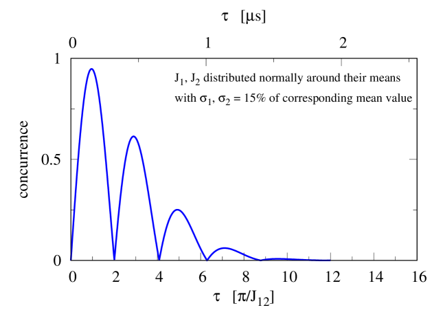
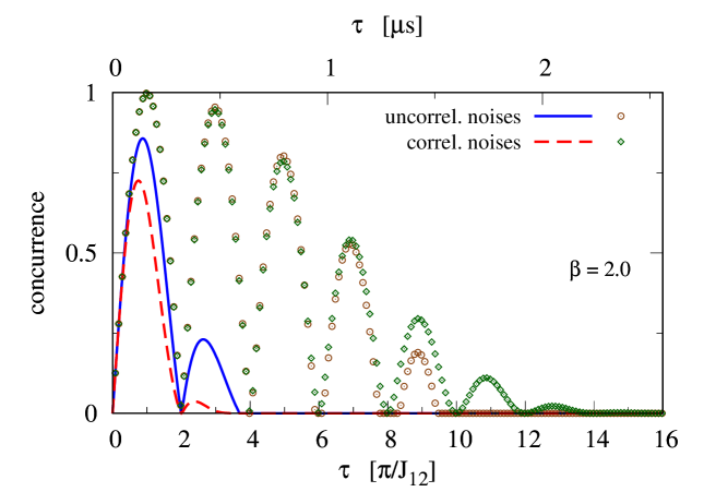
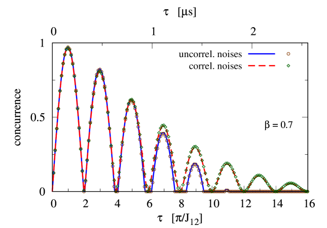
Figure 5: (Color online) Concurrence of the two-qubit state $\langle\hat{\rho}(\tau)\rangle$ as a function of the duration $\tau$ of the entanglement generation procedure. Lines are results for the case in which fluctuations of $J_{i}$ and $J_{12}$ are taken into account, while results in which the fluctuations of $J_{12}$ were artificially turned off are shown with open symbols. Top panel: The case of quasistatically fluctuating $J_{1}$, $J_{2}$ with standard deviations $\sigma_{i}=0.15\bar{J}_{i}$ (Eq. (32)). Middle and bottom panels: The cases of dynamically fluctuating $J_{1}$, $J_{2}$, and hence $J_{12}$, due to $1/f^{\beta}$ noise that is uncorrelated (blue solid line) or perfectly correlated (red dashed lines) for the two qubits. The power of the noise affecting each qubit was chosen to be such that ensures the time scale of decay of single-qubit SE signal like in the experiment [49]: $S$-$T_{0}$ qubit having $J\!=\!1.16$ $\mu$eV shows $T_{\mathrm{SE}}\approx 1.6~{}\mu s$, $S$-$T_{0}$ qubit having $J\!=\!1.32$ $\mu$eV shows $T_{\mathrm{SE}}\approx 1.4~{}\mu s$.

Owing to the fact that the approximated Hamiltonian is diagonal, the density operator undergoes the decoherence of pure dephasing type. There are two essentially distinct types of off-diagonal elements of two-qubit density operator. The density operator elements with a single spin flip: $\langle\rho_{11,1-1}(\tau)\rangle$, $\langle\rho_{11,-11}(\tau)\rangle$, $\langle\rho_{1-1,-1-1}(\tau)\rangle$, $\langle\rho_{-11,-1-1}(\tau)\rangle$ and their Hermitian conjugated partners diminish mainly due to decrease of single-qubits’ signals $\propto\exp\left(-\frac{1}{2}\chi_{\mathrm{SE}}(\tau)\right)$, whereas elements with two spin flips: $\langle\rho_{11,-1-1}(\tau)\rangle$, $\langle\rho_{1-1,-11}(\tau)\rangle$ and their Hermitian conjugated partners decay two times faster as both qubits make their contribution to the decay $\propto\exp\left(-\chi_{\mathrm{SE}}(\tau)\right)$. Hence, the scale on which one can expect the generation of entangled state is limited from above by the single-qubit SE decay time.

In the case of correlated noises, $J_{i}(t)=\bar{J}_{i}+s_{i}\delta J(t)$, the averaged density operator elements are of the following form:

$$\langle\rho_{ab,cd}(\tau)\rangle=\langle\langle ab|\hat{\rho}(\tau)|cd\rangle\rangle$$

$$=\rho_{-a-b,-c-d}^{\mathrm{initial}}\mathrm{e}^{-i\frac{\bar{J}_{1}\bar{J}_{2}}{4K}(ab-cd)\tau}$$

$$\times\left\langle\exp\Big{[}-\frac{i}{2}\Big{\{}\frac{s_{1}\bar{J}_{2}+s_{2}\bar{J}_{1}}{2K}(ab-cd)\right.$$

$$\times\int_{0}^{\tau}\mathrm{d}t\,\delta J(t)f_{\mathrm{FID}}(t)$$

$$+\Big{(}s_{1}\big{(}c-a+\frac{\bar{J}_{2}}{2K}(c+d-a-b)\big{)}$$

$$+s_{2}\big{(}d-b+\frac{\bar{J}_{1}}{2K}(c+d-a-b)\big{)}\Big{)}$$

$$\left.\times\int_{0}^{\tau}\mathrm{d}t\,\delta J(t)f_{\mathrm{SE}}(t)\Big{\}}\Big{]}\right\rangle$$ (42)

$$=\rho_{-a-b,-c-d}^{\mathrm{initial}}\mathrm{e}^{-i\frac{\bar{J}_{1}\bar{J}_{2}}{4K}(ab-cd)\tau}$$

$$\times\exp\Big{[}-\frac{1}{2}\Big{\{}\Big{(}\frac{s_{1}\bar{J}_{2}+s_{2}\bar{J}_{1}}{4K}(ab-cd)\Big{)}^{2}\chi_{\mathrm{FID}}(\tau)$$

$$+\Bigg{(}\frac{1}{2}\Big{(}s_{1}\big{(}c-a+\frac{\bar{J}_{2}}{2K}(c+d-a-b)\big{)}$$

$$+s_{2}\big{(}d-b+\frac{\bar{J}_{1}}{2K}(c+d-a-b)\big{)}\Big{)}\Bigg{)}^{2}\chi_{\mathrm{SE}}(\tau)\Big{\}}\Big{]}.$$ (43)

The key qualitative feature of Eqs. (39) and (43) is the presence of terms proportional to $\chi_{\mathrm{SE}}$, in which the low-frequency noise is suppressed by the echo procedure, and of terms proportional to $\chi_{\mathrm{FID}}$, related to fluctuations of interqubit interaction, in which the low-frequency noise spectrum fully contributes to dephasing.

In Fig. 5 the amount of entanglement is presented in the case of uncorrelated noises for two exponents characterizing $1/f^{\beta}$ noise, $\beta=2.0$ and $0.7$ (middle and bottom panels, respectively). As can be seen in the bottom panel of Fig. 5, for $\beta\!<\!1$ the decay of the overall efficiency of the entangling procedure is mainly caused by influence of fluctuations of splittings of individual qubits (which also fully determines the decay of the fidelity of single-qubit coherence). On the other hand, for $\beta>1$, (e.g. $\beta=2.0$, the middle panel of Fig. 5), the decay of the overall entanglement generation efficiency is mostly due to the infidelity of the entangling gate, which is realized by dynamically fluctuating two-qubit term. This is due to the fact that for noise that is very strongly concentrated at lowest frequencies, single-qubit noise is very efficiently suppressed by the echo procedure, and the non-echoed fluctuations of two-qubit interaction, which are the sources of terms $\propto\chi_{\mathrm{FID}}/K$ in the above expressions for two-qubit coherences, are dominating the dephasing of the final state. Thus, the effect of dynamical noise of $J_{i}$ with high value of $\beta$ on the final state is qualitatively the same as that of quasistatic fluctuations of splittings $J_{i}$ (see the top panel of Fig. 5)), where single-qubit terms cancel out perfectly (thanks to applying Hahn echo on each qubit) and the fidelity of two-qubit entangling gate, which is susceptible to fluctuations as in FID experiment, is diminishing when the duration $\tau$ of the procedure becomes longer.

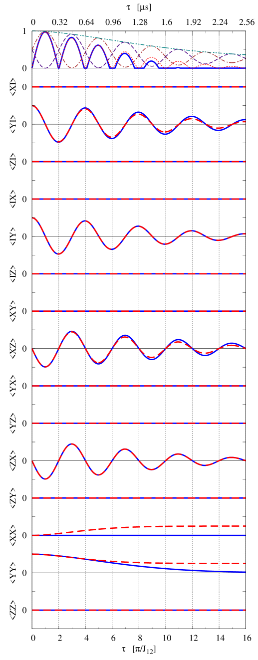
Figure 6: (Color online) Pauli set for the case of $1/f^{0.7}$ noise. Blue lines show calculated Pauli set for two independent noises of $J_{1}(t),J_{2}(t)$, red lines show calculated Pauli set for correlated noises $J_{1}(t)=J_{2}(t)$. In the top panel for the case of independent noises the following measures are shown: blue solid line is concurrence of $\langle\hat{\rho}(\tau)\rangle$, brown dashed line is fidelity $\langle\psi_{\mathrm{o}}|\langle\hat{\rho}(\tau)\rangle|\psi_{\mathrm{o}}\rangle$ (see Eq. (27)), purple dash-dotted line is fidelity $\langle\psi_{\mathrm{e}}|\langle\hat{\rho}(\tau)\rangle|\psi_{\mathrm{e}}\rangle$ (see Eq. (28)), turquoise dotted line is fidelity $\langle\psi(\tau)|\langle\hat{\rho}(\tau)\rangle|\psi(\tau)\rangle$ (see Eq. (26); and red dotted line is concurrence calculated for correlated noises $J_{1}(t)=J_{2}(t)$. The power of the noise affecting each qubit was chosen to be such that ensures the time scale of decay of single-qubit SE signal like in the experiment [49]: $S$-$T_{0}$ qubit having $J\!=\!1.16$ $\mu$eV shows $T_{\mathrm{SE}}\approx 1.6~{}\mu s$, $S$-$T_{0}$ qubit having $J\!=\!1.32$ $\mu$eV shows $T_{\mathrm{SE}}\approx 1.4~{}\mu s$. In the case of fully correlated noises $J_{1}(t)=J_{2}(t)$, the higher power of the noise has been chosen for both qubits.

In Fig. 6 the two Pauli sets for two-qubit states created in the entangling procedure are presented for the case of two uncorrelated $1/f^{0.7}$ noises (blue lines) and for the case of two fully correlated $1/f^{0.7}$ noises (red lines). In noise-free experiment, one expects that the only nonzero two-qubit correlations $\langle\hat{\sigma}_{i}\otimes\hat{\sigma}_{j}\rangle=\mathrm{Tr}\{\left(\hat{\sigma}_{i}\otimes\hat{\sigma}_{j}\right)\hat{\rho}(\tau)\}$ are

$$\langle\hat{\sigma}_{x}\otimes\hat{\sigma}_{z}\rangle =\langle\hat{\sigma}_{z}\otimes\hat{\sigma}_{x}\rangle=-\sin J_{12}\frac{\tau}{2},$$ (44)

$$\langle\hat{\sigma}_{z}\otimes\mathds{1}\rangle =\langle\mathds{1}\otimes\hat{\sigma}_{y}\rangle=\cos J_{12}\frac{\tau}{2},$$ (45)

$$\langle\hat{\sigma}_{y}\otimes\hat{\sigma}_{y}\rangle =1.$$ (46)

Dynamical fluctuations of splittings $J_{i}$ destroy these correlations and diminish their amplitude with increasing duration $\tau$. It is important to notice that fully correlated noises always lead to decreased but nonzero value of $\langle\hat{\sigma}_{y}\otimes\hat{\sigma}_{y}\rangle\stackrel{{\scriptstyle\tau\rightarrow\infty}}{{=}}2\operatorname{\mathrm{Re}}\rho_{1-1,-11}^{\mathrm{initial}}=\frac{1}{2}$, and at the same time new two-qubit correlation $\langle\hat{\sigma}_{x}\otimes\hat{\sigma}_{x}\rangle\stackrel{{\scriptstyle\tau\rightarrow\infty}}{{=}}2\operatorname{\mathrm{Re}}\rho_{1-1,-11}^{\mathrm{initial}}=\frac{1}{2}$ is generated. Therefore, the spatial correlations of noises can have a visible impact on the evolution of resulting state $\hat{\rho}(\tau)$ and components of Pauli set. Hence, one can make use of this fact to estimate to what degree the noises were correlated in the experiment. By comparison of experimental data (Fig. 3 in Ref. [39]) with simulated results (Fig. 6) one may deduce that in the experiment [39] noises of splittings $J_{1}$ and $J_{2}$ were uncorrelated.

VI Conclusions

We have theoretically analyzed the creation and evolution of entanglement of two double quantum dot-based $S$-$T_{0}$ qubits measured in Ref. [39] while taking into account realistic charge and nuclear noise affecting the qubits. We have confirmed that it is possible to have nearly maximal coherence signal of a single $S$-$T_{0}$ qubit in the presence of quasistatic fluctuations of either exchange splitting $J$ or magnetic-field gradient $\Delta B_{z}$ by performing spin echo procedure on the qubit. Then, we have shown that in the system of two $S$-$T_{0}$ qubits quasistatic fluctuations of $\Delta B_{z,i}$ lead only to partial decrease of overall efficiency of the entangling procedure due to imprecise rotations of the qubits’ states.

Both quasistatic or dynamical fluctuations of exchange splittings $J_{1},~{}J_{2}$, and two-qubit coupling $J_{12}\propto J_{1}J_{2}$ lead to decay of overall efficiency of the entangling procedure with increasing its duration $\tau$. The level of correlation of charge noises, as well as their exact functional form (i.e. value of parameter $\beta$ characterizing the $1/f^{\beta}$ noise affecting $J$) translates in a distinctive manner into the shape of decay of two-qubit entanglement as a function of procedure duration $\tau$. Decay of the overall efficiency of entangling procedure may arise as a result of the infidelity of single qubit operations (due to dynamical fluctuations of splittings $J_{1},~{}J_{2}$) or may be caused by infidelity of entangling gate (due to fluctuations of two-qubit coupling $J_{12}$).

Comparison of experimental data from Ref. [39] with our calculations shows that the charge noises in the system of two $S$-$T_{0}$ qubit investigated there were uncorrelated. The main reason of the decreased level of entanglement of the resulting two-qubit state is infidelity of single-qubit operations (as we have obtained for $1/f^{\beta}$ noise with $\beta\!=\!0.7$ consistent with noise observed in other experiments [49] on samples similar to those used in Ref. [39]), whereas contribution of the non-ideal two-qubit gate is negligible in the considered entangling procedure in the regime $\Delta B_{z,i}\ll J_{i}$. We predict that for $J$ noises of more prominently low-frequency character (i.e. $1/f^{\beta}$ with $\beta$ closer to $2$ than $1$), the fluctuations of the two-qubit interactions, which are not echoed by $\pi$ pulses applied to the two qubits separately, will become the main factor suppressing the maximal entanglement achievable in the considered procedure. We have also identified qualitative features of long-time behavior of two-qubit observables from the Pauli set that should be visible when the exchange splitting noises for the two qubits are correlated.

Appendix A Components of a Single $S$-$T_{0}$ Qubit as Functions of Duration $\tau$

In the ideal case, FID signals (i.e. average $\langle\hat{\sigma}_{i}^{\mathrm{FID}}(\tau)\rangle$ components of $S$-$T_{0}$ qubit) evolve as follows.

$$\langle\hat{\sigma}_{x}^{\mathrm{FID}}(\tau)\rangle=\langle{-y}|\mathrm{e}^{i\hat{H}\tau}\hat{\sigma}_{x}\mathrm{e}^{-i\hat{H}\tau}|{-y}\rangle$$

$$=\langle{-y}|\Bigg{(}\cos\Big{(}\frac{\tau}{2}\sqrt{\Delta B_{z}^{2}+J^{2}}\Big{)}\mathds{1}$$

$$+i\sin\Big{(}\frac{\tau}{2}\sqrt{\Delta B_{z}^{2}+J^{2}}\Big{)}\frac{\Delta B_{z}}{\sqrt{\Delta B_{z}^{2}+J^{2}}}\hat{\sigma}_{x}$$

$$+i\sin\Big{(}\frac{\tau}{2}\sqrt{\Delta B_{z}^{2}+J^{2}}\Big{)}\frac{J}{\sqrt{\Delta B_{z}^{2}+J^{2}}}\hat{\sigma}_{z}\Bigg{)}$$

$$\times\hat{\sigma}_{x}\Bigg{(}\cos\Big{(}\frac{\tau}{2}\sqrt{\Delta B_{z}^{2}+J^{2}}\Big{)}\mathds{1}$$

$$-i\sin\Big{(}\frac{\tau}{2}\sqrt{\Delta B_{z}^{2}+J^{2}}\Big{)}\frac{\Delta B_{z}}{\sqrt{\Delta B_{z}^{2}+J^{2}}}\hat{\sigma}_{x}$$

$$-i\sin\Big{(}\frac{\tau}{2}\sqrt{\Delta B_{z}^{2}+J^{2}}\Big{)}\frac{J}{\sqrt{\Delta B_{z}^{2}+J^{2}}}\hat{\sigma}_{z}\Bigg{)}|{-y}\rangle$$

$$=\frac{J}{\sqrt{\Delta B_{z}^{2}+J^{2}}}\sin\Big{(}\sqrt{\Delta B_{z}^{2}+J^{2}}\tau\Big{)}.$$ (47)

$$\langle\hat{\sigma}_{y}^{\mathrm{FID}}(\tau)\rangle =-\cos\Big{[}\sqrt{\Delta B_{z}^{2}+J^{2}}\tau\Big{]}$$ (48)

$$\approx-\cos\Big{[}\left(J+\frac{\Delta B_{z}^{2}}{2J}\right)\tau\Big{]},$$ (49)

the approximation is good for $\tau\ll\frac{8J^{3}}{\Delta B_{z}^{4}}$.

$$\langle\hat{\sigma}_{z}^{\mathrm{FID}}(\tau)\rangle=-\frac{\Delta B_{z}}{\sqrt{\Delta B_{z}^{2}+J^{2}}}\sin\Big{(}\sqrt{\Delta B_{z}^{2}+J^{2}}\tau\Big{)}.$$ (50)

In the ideal case, SE signals (i.e. average $\langle\hat{\sigma}_{i}^{\mathrm{SE}}(\tau)\rangle$ components of $S$-$T_{0}$ qubit) evolve as follows.

$$\langle\hat{\sigma}_{x}^{\mathrm{SE}}(\tau)\rangle =\langle{-y}|\mathrm{e}^{i\hat{H}\frac{\tau}{2}}(i\hat{\sigma}_{x})\mathrm{e}^{i\hat{H}\frac{\tau}{2}}\hat{\sigma}_{x}$$

$$\times\mathrm{e}^{-i\hat{H}\frac{\tau}{2}}(-i\hat{\sigma}_{x})\mathrm{e}^{-i\hat{H}\frac{\tau}{2}}|{-y}\rangle$$

$$=\frac{8\Delta B_{z}^{2}J}{(\Delta B_{z}^{2}+J^{2})^{3/2}}\cos\Big{(}\frac{1}{4}\sqrt{\Delta B_{z}^{2}+J^{2}}\tau\Big{)}$$

$$\times\sin^{2}\Big{(}\frac{1}{4}\sqrt{\Delta B_{z}^{2}+J^{2}}\tau\Big{)}.$$ (51)

$$\langle\hat{\sigma}_{y}^{\mathrm{SE}}(\tau)\rangle =\frac{1}{\Delta B_{z}^{2}+J^{2}}$$

$$\times\Big{(}J^{2}+\Delta B_{z}^{2}\cos\Big{(}\sqrt{\Delta B_{z}^{2}+J^{2}}\tau\Big{)}\Big{)}.$$ (52)

$$\langle\hat{\sigma}_{z}^{\mathrm{SE}}(\tau)\rangle =\frac{\Delta B_{z}}{(\Delta B_{z}^{2}+J^{2})^{3/2}}$$

$$\times\left[2J^{2}\sin^{2}\left(\frac{1}{2}\sqrt{\Delta B_{z}^{2}+J^{2}}\tau\right)\right.$$

$$+\left.\Delta B_{z}^{2}\sin\left(\sqrt{\Delta B_{z}^{2}+J^{2}}\tau\right)\right].$$ (53)

Assuming that $\bar{J}\gg\overline{\Delta B_{z}},\,\sigma_{J}$, after averaging over quasistatic fluctuations of the parameter $\Delta B_{z}$ or $J$ one obtains following approximate expressions for $y$ qubit component during SE.

$$\langle\langle\hat{\sigma}_{y}^{\mathrm{SE}}(\tau)\rangle\rangle_{\Delta B_{z}} \approx\frac{J^{2}}{J^{2}+\overline{\Delta B_{z}}^{2}}$$

$$+\frac{1}{J^{2}+\overline{\Delta B_{z}}^{2}}\exp\left(-\frac{\overline{\Delta B_{z}}^{2}\sigma_{\Delta B_{z}}^{2}\tau^{2}}{2(J^{2}+(\sigma_{\Delta B_{z}}^{2}\tau)^{2})}\right)$$

$$\times\Bigg{[}\frac{J^{3/2}(J(\overline{\Delta B_{z}}^{2}+\sigma_{\Delta B_{z}}^{2})+i\sigma_{\Delta B_{z}}^{4}\tau)}{2(J+i\sigma_{\Delta B_{z}}^{2}\tau)^{5/2}}\Bigg{.}$$

$$\times\exp\left(-iJ\tau\frac{\overline{\Delta B_{z}}^{2}+2J^{2}+2(\sigma_{\Delta B_{z}}^{2}\tau)^{2}}{2(J^{2}+(\sigma_{\Delta B_{z}}^{2}\tau)^{2})}\right)$$

$$\Bigg{.}+\,\mathrm{c.c.}\Bigg{]}.$$ (54)

$$\langle\langle\hat{\sigma}_{y}^{\mathrm{SE}}(\tau)\rangle\rangle_{J} \approx\frac{\bar{J}^{2}+\sigma_{J}^{2}}{\bar{J}^{2}+\Delta B_{z}^{2}}$$

$$+\frac{\Delta B_{z}^{2}}{\bar{J}^{2}+\Delta B_{z}^{2}}\exp\left(-\frac{\sigma_{J}^{2}\tau^{2}}{2}\right)\cos\left(\bar{J}\tau\right).$$ (55)

Appendix B $S$-$T_{0}$ Qubit Attenuation Factors Derived for Dynamically Fluctuating Exchange Splitting

We present the calculation of the attenuation factors $\chi_{\mathrm{FID}}(\tau)$ and $\chi_{\mathrm{SE}}(\tau)$ that account for the effect of dynamically fluctuating exchange splitting $J$. The attenuation factor $\chi_{\mathrm{FID}}(\tau)$ is calculated as follows.

$$\chi_{\mathrm{FID}}(\tau) =\int_{0}^{\tau}\mathrm{d}t_{1}\int_{0}^{\tau}\mathrm{d}t_{2}\langle\delta J(t_{1})\delta J(t_{2})\rangle f_{\mathrm{FID}}(t_{1})f_{\mathrm{FID}}(t_{2})$$

$$=\int_{-\infty}^{\infty}\mathrm{d}t_{1}\int_{-\infty}^{\infty}\mathrm{d}t_{2}\int_{-\infty}^{\infty}\frac{\mathrm{d}\omega}{2\pi}\mathrm{e}^{-i\omega(t_{1}-t_{2})}S(\omega)$$

$$\times\int_{-\infty}^{\infty}\frac{\mathrm{d}\omega_{1}}{2\pi}\tilde{f}_{\mathrm{FID}}(\omega_{1})\mathrm{e}^{-i\omega_{1}t_{1}}\int_{-\infty}^{\infty}\frac{\mathrm{d}\omega_{2}}{2\pi}\tilde{f}_{\mathrm{FID}}(\omega_{2})\mathrm{e}^{-i\omega_{2}t_{2}}$$

$$=\int_{-\infty}^{\infty}\mathrm{d}\omega_{1}\int_{-\infty}^{\infty}\mathrm{d}\omega_{2}\int_{-\infty}^{\infty}\frac{\mathrm{d}\omega}{2\pi}\delta(\omega+\omega_{1})\delta(\omega-\omega_{2})$$

$$\times\tilde{f}_{\mathrm{FID}}(\omega_{1})\tilde{f}_{\mathrm{FID}}(\omega_{2})S(\omega)$$

$$=\int_{-\infty}^{\infty}\frac{\mathrm{d}\omega}{2\pi}\tilde{f}_{\mathrm{FID}}(-\omega)\tilde{f}_{\mathrm{FID}}(\omega)S(\omega)=\int_{-\infty}^{\infty}\frac{\mathrm{d}\omega}{2\pi}\left|\tilde{f}_{\mathrm{FID}}(\omega)\right|^{2}S(\omega)$$

$$=\int_{-\infty}^{\infty}\frac{\mathrm{d}\omega}{2\pi}\frac{2F_{\mathrm{FID}}(\omega\tau)}{\omega^{2}}S(\omega)=2\int_{0}^{\infty}\frac{\mathrm{d}\omega}{\pi}\frac{F_{\mathrm{FID}}(\omega\tau)}{\omega^{2}}S(\omega).$$ (56)

Using the explicit analytical expressions for the filter function $F_{\mathrm{FID}}(\omega\tau)=2\sin^{2}\frac{\omega\tau}{2}$ and the spectral density of the noise $S(\omega)=\frac{A}{\omega^{\beta}}$, where $A$ is a constant corresponding to the power of the noise, we obtain the following expression for the attenuation factor

$$\chi_{\mathrm{FID}}(\tau)=\frac{4A}{\pi}\int_{0}^{\infty}\mathrm{d}\omega\sin^{2}\frac{\omega\tau}{2}\frac{1}{\omega^{2+\beta}},$$ (57)

which for $\beta=0.7$ can be evaluated giving finally:

$$\chi_{\mathrm{FID}}(\tau)=\frac{2A}{\pi}\cos\left(\frac{3\pi}{20}\right)\Gamma\left(-1.7\right)\tau^{1.7}\approx 2.24\,\frac{2A}{\pi}\tau^{1.7},$$ (58)

as the definite integral can be calculated analytically

$$\int_{0}^{\infty}\mathrm{d}\omega\sin^{2}\frac{\omega\tau}{2}\frac{1}{\omega^{2+0.7}}=\frac{1}{2}\cos\left(\frac{3\pi}{20}\right)\Gamma\left(-1.7\right)\tau^{1.7}.$$ (59)

Similarly, the attenuation factor $\chi_{\mathrm{SE}}(\tau)$ reads as follows.

$$\chi_{\mathrm{SE}}(\tau) =\int_{0}^{\tau}\mathrm{d}t_{1}\int_{0}^{\tau}\mathrm{d}t_{2}\langle\delta J(t_{1})\delta J(t_{2})\rangle f_{\mathrm{SE}}(t_{1})f_{\mathrm{SE}}(t_{2})$$

$$=2\int_{0}^{\infty}\frac{\mathrm{d}\omega}{\pi}\frac{F_{\mathrm{SE}}(\omega\tau)}{\omega^{2}}S(\omega).$$ (60)

Using the explicit analytical expressions for the filter function $F_{\mathrm{SE}}(\omega\tau)=8\sin^{4}\frac{\omega\tau}{4}$ and the spectral density of the noise $S(\omega)=\frac{A}{\omega^{\beta}}$, we obtain the following expression for the attenuation factor

$$\chi_{\mathrm{SE}}(\tau)=\frac{16A}{\pi}\int_{0}^{\infty}\mathrm{d}\omega\sin^{4}\frac{\omega\tau}{4}\frac{1}{\omega^{2+\beta}},$$ (61)

which for $\beta=0.7$ can be evaluated giving finally:

$$\chi_{\mathrm{SE}}(\tau)=\frac{2A}{\pi}\left(2^{0.3}-1\right)\cos\left(\frac{3\pi}{20}\right)\Gamma\left(-1.7\right)\tau^{1.7}\approx 0.52\,\frac{2A}{\pi}\tau^{1.7},$$ (62)

as the definite integral can be calculated analytically

$$\int_{0}^{\infty}\mathrm{d}\omega\sin^{4}\frac{\omega\tau}{4}\frac{1}{\omega^{2+0.7}}=\frac{1}{8}\left(2^{0.3}-1\right)\cos\left(\frac{3\pi}{20}\right)\Gamma\left(-1.7\right)\tau^{1.7}.$$ (63)

The attenuation factor $\chi_{\mathrm{SE}}(\tau)$ for noise with $\beta=2.0$ is $\chi_{\mathrm{SE}}(\tau)=\frac{A}{12}\tau^{3}$ as the following definite integral can be calculated analytically $\int_{0}^{\infty}\mathrm{d}\omega\sin^{4}\frac{\omega\tau}{4}\frac{1}{\omega^{2+2.0}}=\frac{\pi}{192}\tau^{3}$.

References

- Hanson et al. [2007] R. Hanson, L. P. Kouwenhoven, J. R. Petta, S. Tarucha, and L. M. K. Vandersypen, Spins in few-electron quantum dots, Rev. Mod. Phys. 79, 1217 (2007).
- Chatterjee et al. [2021] A. Chatterjee, P. Stevenson, S. De Franceschi, A. Morello, N. P. de Leon, and F. Kuemmeth, Semiconductor qubits in practice, Nature Reviews Physics 3, 157 (2021).
- Burkard et al. [2023] G. Burkard, T. D. Ladd, A. Pan, J. M. Nichol, and J. R. Petta, Semiconductor spin qubits, Rev. Mod. Phys. 95, 025003 (2023).
- Loss and DiVincenzo [1998] D. Loss and D. P. DiVincenzo, Quantum computation with quantum dots, Phys. Rev. A 57, 120 (1998).
- Koppens et al. [2006] F. H. L. Koppens, C. Buizert, K. J. Tielrooij, I. T. Vink, K. C. Nowack, T. Meunier, L. P. Kouwenhoven, and L. M. K. Vandersypen, Driven coherent oscillations of a single electron spin in a quantum dot, Nature 442, 766 (2006).
- Nowack et al. [2007] K. C. Nowack, F. H. L. Koppens, Y. V. Nazarov, and L. M. K. Vandersypen, Coherent control of a single electron spin with electric fields, Science 318, 1430 (2007).
- Pioro-Ladrière et al. [2008] M. Pioro-Ladrière, T. Obata, Y. Tokura, Y.-S. Shin, T. Kubo, K. Yoshida, T. Taniyama, and S. Tarucha, Electrically driven single-electron spin resonance in a slanting Zeeman field, Nature Phys 4, 776 (2008).
- Burkard et al. [1999] G. Burkard, D. Loss, and D. P. DiVincenzo, Coupled quantum dots as quantum gates, Phys. Rev. B 59, 2070 (1999).
- Li et al. [2010] Q. Li, Ł. Cywiński, D. Culcer, X. Hu, and S. Das Sarma, Exchange coupling in silicon quantum dots: Theoretical considerations for quantum computation, Phys. Rev. B 81, 085313 (2010).
- Petta et al. [2005] J. R. Petta, A. C. Johnson, J. M. Taylor, E. A. Laird, A. Yacoby, M. D. Lukin, C. M. Marcus, M. P. Hanson, and A. C. Gossard, Coherent manipulation of coupled electron spins in semiconductor quantum dots, Science 309, 2180 (2005).
- Brunner et al. [2011] R. Brunner, Y.-S. Shin, T. Obata, M. Pioro-Ladrière, T. Kubo, K. Yoshida, T. Taniyama, Y. Tokura, and S. Tarucha, Two-qubit gate of combined single-spin rotation and interdot spin exchange in a double quantum dot, Phys. Rev. Lett. 107, 146801 (2011).
- Veldhorst et al. [2015] M. Veldhorst, C. H. Yang, J. C. C. Hwang, W. Huang, J. P. Dehollain, J. T. Muhonen, S. Simmons, A. Laucht, F. E. Hudson, K. M. Itoh, A. Morello, and A. S. Dzurak, A two-qubit logic gate in silicon, Nature 526, 410 (2015).
- Reed et al. [2016] M. D. Reed, B. M. Maune, R. W. Andrews, M. G. Borselli, K. Eng, M. P. Jura, A. A. Kiselev, T. D. Ladd, S. T. Merkel, I. Milosavljevic, E. J. Pritchett, M. T. Rakher, R. S. Ross, A. E. Schmitz, A. Smith, J. A. Wright, M. F. Gyure, and A. T. Hunter, Reduced sensitivity to charge noise in semiconductor spin qubits via symmetric operation, Phys. Rev. Lett. 116, 110402 (2016).
- Martins et al. [2016] F. Martins, F. K. Malinowski, P. D. Nissen, E. Barnes, S. Fallahi, G. C. Gardner, M. J. Manfra, C. M. Marcus, and F. Kuemmeth, Noise suppression using symmetric exchange gates in spin qubits, Phys. Rev. Lett. 116, 116801 (2016).
- Watson et al. [2018] T. F. Watson, S. G. J. Philips, E. Kawakami, D. R. Ward, P. Scarlino, M. Veldhorst, D. E. Savage, M. G. Lagally, M. Friesen, S. N. Coppersmith, M. A. Eriksson, and L. M. K. Vandersypen, A programmable two-qubit quantum processor in silicon, Nature 555, 633 (2018).
- Huang et al. [2019] W. Huang, C. H. Yang, K. W. Chan, T. Tanttu, B. Hensen, R. C. C. Leon, M. A. Fogarty, J. C. C. Hwang, F. E. Hudson, K. M. Itoh, A. Morello, A. Laucht, and A. S. Dzurak, Fidelity benchmarks for two-qubit gates in silicon, Nature 569, 532 (2019).
- Laird et al. [2007] E. A. Laird, C. Barthel, E. I. Rashba, C. M. Marcus, M. P. Hanson, and A. C. Gossard, Hyperfine-mediated gate-driven electron spin resonance, Phys. Rev. Lett. 99, 246601 (2007).
- Coish and Baugh [2009] W. A. Coish and J. Baugh, Nuclear spins in nanostructures, physica status solidi (b) 246, 2203 (2009).
- Cywiński [2011] Ł. Cywiński, Dephasing of electron spin qubits due to their interaction with nuclei in quantum dots, Acta Phys. Pol. A 119, 576 (2011).
- Chekhovich et al. [2013] E. A. Chekhovich, M. N. Makhonin, A. I. Tartakovskii, A. Yacoby, H. Bluhm, K. C. Nowack, and L. M. K. Vandersypen, Nuclear spin effects in semiconductor quantum dots, Nature Mater 12, 494 (2013).
- Yang et al. [2017] W. Yang, W.-L. Ma, and R.-B. Liu, Quantum many-body theory for electron spin decoherence in nanoscale nuclear spin baths, Rep. Prog. Phys. 80, 016001 (2017).
- Kawakami et al. [2016] E. Kawakami, T. Jullien, P. Scarlino, D. R. Ward, D. E. Savage, M. G. Lagally, V. V. Dobrovitski, M. Friesen, S. N. Coppersmith, M. A. Eriksson, and L. M. K. Vandersypen, Gate fidelity and coherence of an electron spin in an Si/SiGe quantum dot with micromagnet, PNAS 113, 11738 (2016).
- Veldhorst et al. [2014] M. Veldhorst, J. C. C. Hwang, C. H. Yang, A. W. Leenstra, B. de Ronde, J. P. Dehollain, J. T. Muhonen, F. E. Hudson, K. M. Itoh, A. Morello, and A. S. Dzurak, An addressable quantum dot qubit with fault-tolerant control-fidelity, Nature Nanotech 9, 981 (2014).
- Yoneda et al. [2018] J. Yoneda, K. Takeda, T. Otsuka, T. Nakajima, M. R. Delbecq, G. Allison, T. Honda, T. Kodera, S. Oda, Y. Hoshi, N. Usami, K. M. Itoh, and S. Tarucha, A quantum-dot spin qubit with coherence limited by charge noise and fidelity higher than 99.9%, Nature Nanotech 13, 102 (2018).
- Struck et al. [2020] T. Struck, A. Hollmann, F. Schauer, O. Fedorets, A. Schmidbauer, K. Sawano, H. Riemann, N. V. Abrosimov, Ł. Cywiński, and D. Bougeard, Low-frequency spin qubit energy splitting noise in highly purified 28Si/SiGe, npj Quantum Inf 6, 40 (2020).
- Higginbotham et al. [2014] A. P. Higginbotham, F. Kuemmeth, M. P. Hanson, A. C. Gossard, and C. M. Marcus, Coherent operations and screening in multielectron spin qubits, Phys. Rev. Lett. 112, 026801 (2014).
- Kim et al. [2014] D. Kim, Z. Shi, C. B. Simmons, D. R. Ward, J. R. Prance, T. S. Koh, J. K. Gamble, D. E. Savage, M. G. Lagally, M. Friesen, S. N. Coppersmith, and M. A. Eriksson, Quantum control and process tomography of a semiconductor quantum dot hybrid qubit, Nature 511, 70 (2014).
- Medford et al. [2013a] J. Medford, J. Beil, J. M. Taylor, S. D. Bartlett, A. C. Doherty, E. I. Rashba, D. P. DiVincenzo, H. Lu, A. C. Gossard, and C. M. Marcus, Self-consistent measurement and state tomography of an exchange-only spin qubit, Nature Nanotech 8, 654 (2013a).
- Medford et al. [2013b] J. Medford, J. Beil, J. M. Taylor, E. I. Rashba, H. Lu, A. C. Gossard, and C. M. Marcus, Quantum-dot-based resonant exchange qubit, Phys. Rev. Lett. 111, 050501 (2013b).
- Russ et al. [2018] M. Russ, J. R. Petta, and G. Burkard, Quadrupolar exchange-only spin qubit, Phys. Rev. Lett. 121, 177701 (2018).
- Sala and Danon [2017] A. Sala and J. Danon, Exchange-only singlet-only spin qubit, Phys. Rev. B 95, 241303 (2017).
- Bluhm et al. [2010a] H. Bluhm, S. Foletti, D. Mahalu, V. Umansky, and A. Yacoby, Enhancing the coherence of a spin qubit by operating it as a feedback loop that controls its nuclear spin bath, Phys. Rev. Lett. 105, 216803 (2010a).
- Foletti et al. [2009] S. Foletti, H. Bluhm, D. Mahalu, V. Umansky, and A. Yacoby, Universal quantum control of two-electron spin quantum bits using dynamic nuclear polarization, Nature Phys 5, 903 (2009).
- Horodecki et al. [2009] R. Horodecki, P. Horodecki, M. Horodecki, and K. Horodecki, Quantum entanglement, Rev. Mod. Phys. 81, 865 (2009).
- Aolita et al. [2015] L. Aolita, F. de Melo, and L. Davidovich, Open-system dynamics of entanglement, Rep. Prog. Phys. 78, 042001 (2015).
- Nowack et al. [2011] K. C. Nowack, M. Shafiei, M. Laforest, G. E. D. K. Prawiroatmodjo, L. R. Schreiber, C. Reichl, W. Wegscheider, and L. M. K. Vandersypen, Single-shot correlations and two-qubit gate of solid-state spins, Science 333, 1269 (2011).
- Taylor et al. [2005] J. M. Taylor, H. A. Engel, W. Dur, A. Yacoby, C. M. Marcus, P. Zoller, and M. D. Lukin, Fault-tolerant architecture for quantum computation using electrically controlled semiconductor spins, Nature Phys 1, 177 (2005).
- van Weperen et al. [2011] I. van Weperen, B. D. Armstrong, E. A. Laird, J. Medford, C. M. Marcus, M. P. Hanson, and A. C. Gossard, Charge-state conditional operation of a spin qubit, Phys. Rev. Lett. 107, 030506 (2011).
- Shulman et al. [2012] M. D. Shulman, O. E. Dial, S. P. Harvey, H. Bluhm, V. Umansky, and A. Yacoby, Demonstration of entanglement of electrostatically coupled singlet-triplet qubits, Science 336, 202 (2012).
- Li et al. [2012] R. Li, X. Hu, and J. Q. You, Controllable exchange coupling between two singlet-triplet qubits, Phys. Rev. B 86, 205306 (2012).
- Wardrop and Doherty [2014] M. P. Wardrop and A. C. Doherty, Exchange-based two-qubit gate for singlet-triplet qubits, Phys. Rev. B 90, 045418 (2014).
- Cerfontaine et al. [2020] P. Cerfontaine, R. Otten, M. A. Wolfe, P. Bethke, and H. Bluhm, High-fidelity gate set for exchange-coupled singlet-triplet qubits, Phys. Rev. B 101, 155311 (2020).
- Hornberger [2009] K. Hornberger, Introduction to decoherence theory, Lecture Notes in Physics 768, 221 (2009).
- Mazurek et al. [2014] P. Mazurek, K. Roszak, R. W. Chhajlany, and P. Horodecki, Sensitivity of entanglement decay of quantum-dot spin qubits to the external magnetic field, Phys. Rev. A 89, 062318 (2014).
- Bragar and Cywiński [2015] I. Bragar and Ł. Cywiński, Dynamics of entanglement of two electron spins interacting with nuclear spin baths in quantum dots, Phys. Rev. B 91, 155310 (2015).
- Bluhm et al. [2010b] H. Bluhm, S. Foletti, I. Neder, M. Rudner, D. Mahalu, V. Umansky, and A. Yacoby, Dephasing time of gaas electron-spin qubits coupled to a nuclear bath exceeding 200 s, Nature Phys 7, 109 (2010b).
- Coish and Loss [2005] W. A. Coish and D. Loss, Singlet-triplet decoherence due to nuclear spins in a double quantum dot, Phys. Rev. B 72, 125337 (2005).
- Hu and Das Sarma [2006] X. Hu and S. Das Sarma, Charge-fluctuation-induced dephasing of exchange-coupled spin qubits, Phys. Rev. Lett. 96, 100501 (2006).
- Dial et al. [2013] O. E. Dial, M. D. Shulman, S. P. Harvey, H. Bluhm, V. Umansky, and A. Yacoby, Charge noise spectroscopy using coherent exchange oscillations in a singlet-triplet qubit, Phys. Rev. Lett. 110, 146804 (2013).
- Yang and Liu [2008] W. Yang and R. B. Liu, Decoherence of coupled electron spins via nuclear spin dynamics in quantum dots, Phys. Rev. B 77, 085302 (2008).
- Hung et al. [2013] J.-T. Hung, Ł. Cywiński, X. Hu, and S. Das Sarma, Hyperfine interaction induced dephasing of coupled spin qubits in semiconductor double quantum dots, Phys. Rev. B 88, 085314 (2013).
- Weiss et al. [2012] K. M. Weiss, J. M. Elzerman, Y. L. Delley, J. Miguel-Sanchez, and A. Imamoğlu, Coherent two-electron spin qubits in an optically active pair of coupled InGaAs quantum dots, Phys. Rev. Lett. 109, 107401 (2012).
- Wu and Das Sarma [2017] Y.-L. Wu and S. Das Sarma, Decoherence of two coupled singlet-triplet spin qubits, Phys. Rev. B 96, 165301 (2017).
- Taylor et al. [2007] J. M. Taylor, J. R. Petta, A. C. Johnson, A. Yacoby, C. M. Marcus, and M. D. Lukin, Relaxation, dephasing, and quantum control of electron spins in double quantum dots, Phys. Rev. B 76, 035315 (2007).
- Reilly et al. [2008] D. J. Reilly, J. M. Taylor, E. A. Laird, J. R. Petta, C. M. Marcus, M. P. Hanson, and A. C. Gossard, Measurement of temporal correlations of the Overhauser field in a double quantum dot, Phys. Rev. Lett. 101, 236803 (2008).
- Wang et al. [2012] X. Wang, L. S. Bishop, J. P. Kestner, E. Barnes, K. Sun, and S. Das Sarma, Composite pulses for robust universal control of singlet-triplet qubits, Nat Commun 3, 997 (2012).
- Kestner et al. [2013] J. P. Kestner, X. Wang, L. S. Bishop, E. Barnes, and S. Das Sarma, Noise-resistant control for a spin qubit array, Phys. Rev. Lett. 110, 140502 (2013).
- Wang et al. [2014] X. Wang, L. S. Bishop, E. Barnes, J. P. Kestner, and S. Das Sarma, Robust quantum gates for singlet-triplet spin qubits using composite pulses, Phys. Rev. A 89, 022310 (2014).
- Nichol et al. [2017] J. M. Nichol, L. A. Orona, S. P. Harvey, S. Fallahi, G. C. Gardner, M. J. Manfra, and A. Yacoby, High-fidelity entangling gate for double-quantum-dot spin qubits, npj Quantum Inf 3, 3 (2017).
- Reilly et al. [2010] D. J. Reilly, J. M. Taylor, J. R. Petta, C. M. Marcus, M. P. Hanson, and A. C. Gossard, Exchange control of nuclear spin diffusion in a double quantum dot, Phys. Rev. Lett. 104, 236802 (2010).
- Yao et al. [2006] W. Yao, R.-B. Liu, and L. J. Sham, Theory of electron spin decoherence by interacting nuclear spins in a quantum dot, Phys. Rev. B 74, 195301 (2006).
- Witzel and Das Sarma [2006] W. M. Witzel and S. Das Sarma, Quantum theory for electron spin decoherence induced by nuclear spin dynamics in semiconductor quantum computer architectures: Spectral diffusion of localized electron spins in the nuclear solid-state environment, Phys. Rev. B 74, 035322 (2006).
- Witzel and Das Sarma [2008] W. M. Witzel and S. Das Sarma, Wavefunction considerations for the central spin decoherence problem in a nuclear spin bath, Phys. Rev. B 77, 165319 (2008).
- Taylor and Lukin [2006] J. M. Taylor and M. D. Lukin, Dephasing of quantum bits by a quasi-static mesoscopic environment, Quantum Inf Process 5, 503 (2006).
- Merkulov et al. [2002] I. A. Merkulov, A. L. Efros, and M. Rosen, Electron spin relaxation by nuclei in semiconductor quantum dots, Phys. Rev. B 65, 205309 (2002).
- Ramon [2012] G. Ramon, Dynamical decoupling of a singlet-triplet qubit afflicted by a charge fluctuator, Phys. Rev. B 86, 125317 (2012).
- Ramon [2015] G. Ramon, Non-gaussian signatures and collective effects in charge noise affecting a dynamically decoupled qubit, Phys. Rev. B 92, 155422 (2015).
- de Sousa [2009] R. de Sousa, Electron spin as a spectrometer of nuclear-spin noise and other fluctuations, Topics in Applied Physics 115, 183 (2009).
- Cywiński et al. [2008] Ł. Cywiński, R. M. Lutchyn, C. P. Nave, and S. Das Sarma, How to enhance dephasing time in superconducting qubits, Phys. Rev. B 77, 174509 (2008).
- Szańkowski et al. [2017] P. Szańkowski, G. Ramon, J. Krzywda, D. Kwiatkowski, and Ł. Cywiński, Environmental noise spectroscopy with qubits subjected to dynamical decoupling, J. Phys.: Condens. Matter 29, 333001 (2017).
- Buterakos et al. [2018] D. Buterakos, R. E. Throckmorton, and S. Das Sarma, Crosstalk error correction through dynamical decoupling of single-qubit gates in capacitively coupled singlet-triplet semiconductor spin qubits, Phys. Rev. B 97, 045431 (2018).
- Nielsen et al. [2012] E. Nielsen, R. P. Muller, and M. S. Carroll, Configuration interaction calculations of the controlled phase gate in double quantum dot qubits, Phys. Rev. B 85, 035319 (2012).
- Chan et al. [2021] G. X. Chan, J. P. Kestner, and X. Wang, Charge noise suppression in capacitively coupled singlet-triplet spin qubits under magnetic field, Phys. Rev. B 103, L161409 (2021).
- Wootters [1998] W. K. Wootters, Entanglement of formation of an arbitrary state of two qubits, Phys. Rev. Lett. 80, 2245 (1998).
- Note [1] For typical values of eV and eV, the angle between the axis and the actual axis of rotations is .
- Note [2] Using a geometrical interpretation of qubit’s state space, one can notice that rotation about axis, , changes the sign of component of the qubit’s Bloch vector. Hence, for example, the maximally distant from the equatorial plane state , where , with corresponding Bloch vector , which is obtained from the initial state after a period of the free evolution (the rotation by about an axis tilted from the direction with both present and ), transforms into with corresponding Bloch vector , where , are the unit vectors of , directions, respectively. The only qubit’s states generated in the free evolution starting from which stay in the equatorial plane after application of are states with corresponding Bloch vectors , where is the unit vector of direction.
- Boter et al. [2020] J. M. Boter, X. Xue, T. Krähenmann, T. F. Watson, V. N. Premakumar, D. R. Ward, D. E. Savage, M. G. Lagally, M. Friesen, S. N. Coppersmith, M. A. Eriksson, R. Joynt, and L. M. K. Vandersypen, Spatial noise correlations in a Si/SiGe two-qubit device from bell state coherences, Phys. Rev. B 101, 235133 (2020).
- Yoneda et al. [2022] J. Yoneda, J. S. Rojas-Arias, P. Stano, K. Takeda, A. Noiri, T. Nakajima, D. Loss, and S. Tarucha, Noise-correlation spectrum for a pair of spin qubits in silicon, arXiv:2208.14150 10.48550/ARXIV.2208.14150 (2022).