Continuous-time Autoencoders for Regular and Irregular Time Series Imputation

Abstract.

Time series imputation is one of the most fundamental tasks for time series. Real-world time series datasets are frequently incomplete (or irregular with missing observations), in which case imputation is strongly required. Many different time series imputation methods have been proposed. Recent self-attention-based methods show the state-of-the-art imputation performance. However, it has been overlooked for a long time to design an imputation method based on continuous-time recurrent neural networks (RNNs), i.e., neural controlled differential equations (NCDEs). To this end, we redesign time series (variational) autoencoders based on NCDEs. Our method, called continuous-time autoencoder (CTA), encodes an input time series sample into a continuous hidden path (rather than a hidden vector) and decodes it to reconstruct and impute the input. In our experiments with 4 datasets and 19 baselines, our method shows the best imputation performance in almost all cases.

1. Introduction

Time series is one of the most frequently occurring data formats in real-world applications, and there exist many machine learning tasks related to time series, ranging from stock price forecasting to weather forecasting (Khare et al., 2017; Vargas et al., 2017; Dingli and Fournier, 2017; Jiang, 2021; Sen and Mehtab, 2021; Hwang et al., 2021; Choi et al., 2023; Karevan and Suykens, 2020; Hewage et al., 2020; Yu et al., 2017; Wu et al., 2019; Fang et al., 2021; Li and Zhu, 2021; Tekin et al., 2021; Zeng et al., 2022; Zhou et al., 2021; Shi et al., 2015). These applications frequently assume complete time series. In reality, however, time series can be incomplete with missing observations, e.g., a weather station’s sensors are damaged for a while. As a matter of fact, many famous benchmark datasets for time series forecasting/classification are pre-processed with imputation methods to make them complete, e.g., (Chen et al., 2001; Jiang and Luo, 2022; Choi et al., 2022; Choi and Park, 2023). In this regard, time series imputation is one of the most fundamental topics in the field of time series processing. However, its difficulty lies in that i) time series is incomplete since some elements are missing and moreover, ii) the missing rate can be sometimes high, e.g., (Silva et al., 2012).

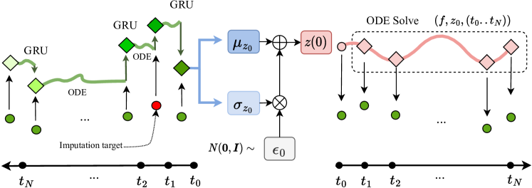
(a) Latent ODE (Rubanova et al., 2019) produces a hidden vector $\mathbf{z}(0)$ given a time series input. We note that the decoder of Latent ODE reverts the sequence of the input, and only one pair of $(\boldsymbol{\mu},\boldsymbol{\sigma})$ is produced. The incomplete observation in red is first pre-processed by setting missing elements to zeros.

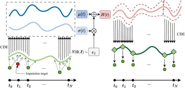
(b) Our proposed CTA, whose encoder/decoder are NCDEs, produces a continuous hidden path $H(t),t\in{[}t_{0},t_{N}{]}$. Given a discrete time series sample, the encoder first interpolates it to estimate its continuous data path (highlighted in light green) and then evolves its state vector, i.e., ${[}\boldsymbol{\mu}(t),\boldsymbol{\sigma}(t){]}$ in this example, via the Riemann–Stieltjes integral. The decoder reconstructs and imputes for the original incomplete time series sample. Since ${[}\boldsymbol{\mu}(t),\boldsymbol{\sigma}(t){]}$ is defined continuously over time, one can consider that there exist infinitely many autoencoders between $t_{0}$ and $t_{N}$ (cf. Fig.2).

Figure 1. Overall workflow of Latent ODE and our method, CTA, to impute incomplete observations in red.

Table 1. Comparison of methods in terms of i) how to process irregular time series, and ii) how to process the missing value of the original data, and iii) whether the time can be handled continuously

Model	irregular time series	missing value	continuous time
BRITS (Cao et al., 2018)	time decay	fill zero	X
GP-VAE (Fortuin et al., 2020)	raw timestamp
GAIN (Yoon et al., 2018a)	X
SAITS (Du et al., 2023)	positional encoding
CTA	neural controlled differential equation		O

To this end, diverse approaches have been proposed, ranging from simple interpolations to deep learning-based methods. Those deep learning-based methods can be further categorized into recurrent neural network-based (Suo et al., 2019; Yoon et al., 2018b; Che et al., 2018; Cao et al., 2018), variational autoencoder-based (Rubanova et al., 2019; Fortuin et al., 2020; Nazabal et al., 2020), generative adversarial networks-based (Yoon et al., 2018a; Luo et al., 2018, 2019), self-attention-based (Ma et al., 2019; Shan et al., 2021; Shukla and Marlin, 2020, 2021; Du et al., 2023), and some others. Among them, self-attention-based methods, e.g., SAITS (Du et al., 2023), show the state-of-the-art imputation quality. SAITS adopts dual layers of transformers since the time series imputation is challenging and therefore, a single layer of transformer is not sufficient.

Our approach:

In this work, we propose the concept of Continuous-Time Autoencoder (CTA) to impute time series. We, for the first time, extend (variational) autoencoders for processing time series in a continuous manner — there already exist some other non-continuous-time autoencoders for time series, e.g., Latent ODE (Rubanova et al., 2019). To enable our concept, we resort to neural controlled differential equations (NCDEs) which are considered as continuous-time recurrent neural networks (RNNs) (Hochreiter and Schmidhuber, 1997; Cho et al., 2014). The overall framework follows the (variational) autoencoder architecture (Kingma and Welling, 2013) with an NCDE-based encoder and decoder (see Fig. 1(b)). Since time series for imputation is inevitably irregular with missing elements, our method based on continuous-time RNNs, i.e., NCDEs, is suitable for the task.

Table 1 summarizes how the state-of-the-art RNN, VAE, GAN, and transformer-based imputation models process irregular and incomplete time series inputs — existing methods primarily focus on regular time series and process irregular time series with heuristics, e.g., time decay. BRITS gives a decay on the time lag, and GP-VAE uses the raw timestamp as an additional feature. The temporal information is not used in GAIN, and SAITS adopts the positional encoding within its transformer. Moreover, they fill out missing values simply with zeros, which introduces noises into the data distribution. To address these limitations, our proposed method resorts to the NCDE technology by creating the continuous hidden path with irregular time series inputs. By modeling the hidden dynamics of time series in a continuous manner, in addition, our method is able to learn robust representations.

Figure 2. We highlight the encoder part from Fig. 1(b).

An infinite number of autoencoders:

Our approach differs from other (variational) autoencoder-based approaches for time series that encode a time series sample into a single hidden vector and decodes it (cf. Fig. 1(a) where $\mathbf{z}(0)$ is produced by the encoder). As shown in Fig. 1(b), however, we define an autoencoder for every time $t\in[t_{0},t_{N}]$ given a time series sample. In other words, there exist infinitely many autoencoders in $[t_{0},t_{N}]$ since we can define $[\boldsymbol{\mu}(t),\boldsymbol{\sigma}(t)]$ for every single time point $t$. At the end, the continuous hidden path $H(t)$ is produced (rather than a vector). Therefore, one can consider that our method is a continuous generalization of (variational) autoencoders — our method is able to continuously generalize both variational and vanilla autoencoders.

Hidden vector vs. hidden path:

Compared to the single hidden vector approach, our method has much flexibility in encoding an input time series sample. Since the single hidden vector may not be able to compress all the information contained by the input, it may selectively encode some key information only and this task can be difficult sometimes. However, our method encodes the input into a continuous path that has much higher representation flexibility.

Dual layer and training with missing values:

Existing time series imputation methods have various architectures. However, some highly performing methods have dual layers of transformers, e.g., SAITS, and being inspired by them, we also design i) a special architecture for our method and ii) its training algorithm. We carefully connects two continuous-time autoencoders (CTAs) via a learnable weighted sum method, i.e., we learn how to combine those two CTAs. Since our CTA can be either variational or vanilla autoencoder, we test all four combinations of them, i.e., two options for each layer. In general, VAE-AE or AE-AE architectures show good performance, where VAE means variational autoencoder and AE means vanilla autoencoder, and the sequence separated by the hyphen represents the layered architecture. In addition, we train the proposed dual-layered architecture with our proposed special training method with missing elements. We intentionally remove some existing elements to create imputation environments for training.

We conduct time series imputation experiments with 4 datasets and 19 baselines. In almost all cases, our CTA shows the best accuracy and its model size is also much lower than the state-of-the-art baseline. Our contributions can be summarized as follows:

1. We generalize (variational) autoencoders in a continuous manner. Therefore, the encoder in our proposed method creates a continuous path $H(t)$ of latent representations, from which our decoder reconstructs the original time series and imputes missing elements. Our continuous hidden path $H(t)$ is able to encode rich information.

2. We test with various missing rates from 30% to 70% on 4 datasets. Our method consistently outperforms baselines in most cases, owing to the continuous RNNs, i.e., NCDEs.

2. Preliminaries & Related Work

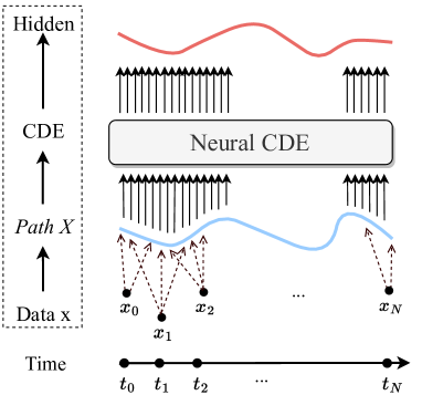
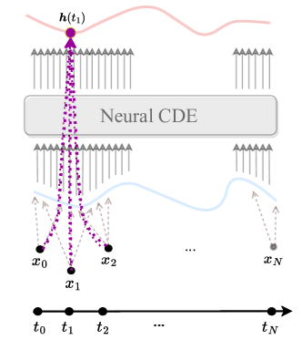
Figure 3. Overall workflow of NCDEs. In (a), after creating the continuous path $X(t)$, every computation works in the continuous time domain. When calculating $\boldsymbol{h}(t_{1})$ in (b), observations around $t_{1}$ are considered via the interpolated continuous path $X(t)$ — some sparse transformers also consider a small number of neighboring observations in a discrete time domain (Tay et al., 2022).

2.1. Neural Controlled Differential Equations

NCDEs solve the following initial value problem (IVP) based on the Riemann-Stieltjes integral problem (Stieltjes, 1894) to derive the hidden state $\boldsymbol{h}(T)$ from the initial state $\boldsymbol{h}(0)$:

(1) $$\boldsymbol{h}(T) =\boldsymbol{h}(0)+\int_{0}^{T}f(\boldsymbol{h}(t),t;\boldsymbol{\theta}_{f})dX,$$

(2) $$=\boldsymbol{h}(0)+\int_{0}^{T}f(\boldsymbol{h}(t),t;\boldsymbol{\theta}_{f})\frac{dX(t)}{dt}dt,$$

where $X(t)$ is a path representing the continuous input. In general, $X(t)$ is estimated from its discrete time series $\{(\mathbf{x}_{i},t_{i})\}_{i=0}^{N}$ via an interpolation method, where $\mathbf{x}_{i}$ is a multivariate observation at time $t_{i}$, e.g., given discrete sensing results of weather stations, we reconstruct their continuous path via an interpolation method — the natural cubic spline method (McKinley and Levine, 1998; Kidger et al., 2020) is frequently used for NCDEs since it is twice differentiable when calculating the gradient w.r.t. $\boldsymbol{\theta}_{f}$. For this reason, NCDEs are called as continuous RNNs — one can consider that the hidden state $\boldsymbol{h}(t)$ of RNNs continuously evolves from $t=0$ to $T$ while reading the input $\frac{dX(t)}{dt}$ in NCDEs (cf. Fig. 3). Since NCDEs create $X(t)$ via the interpolation method, however, the hidden state $\boldsymbol{h}(t)$ at time $t$ is created by considering input observations around $t$ (cf. Fig. 3), which is one subtle but important difference from conventional RNNs.

The above IVP of NCDEs can be solved with existing ODE solvers, since $\frac{d\boldsymbol{h}(t)}{dt}=f(\boldsymbol{h}(t),t,\theta_{f})\frac{dX(t)}{dt}$. For instance the explicit Euler method, the simplest ODE solver, solves the above IVP by iterating the following step multiple times from $t=0$ to $T$:

(3) $$\boldsymbol{h}(t+s) =\boldsymbol{h}(t)+s\frac{d\boldsymbol{h}(t)}{dt}=\boldsymbol{h}(t)+sf(\boldsymbol{h}(t),t,\theta_{f})\frac{dX(t)}{dt},$$

where $s$ is a pre-configured step size.

2.2. Time Series Imputation

2.2.1. RNN-based

Existing RNN-based models regard timestamps as one attributes of raw data. GRU-D (Che et al., 2018) proposes the concept of time lag and imputes missing elements with the weighted combination of its last observation and the global mean with time decay. However, such assumption has limitations on general datasets. M-RNN (Yoon et al., 2018b) proposes the multi-directional RNN to impute random missing elements, which considers both intra-data relationships inside a data stream and inter-data relationships across data streams. M-RNN, however, has no consideration on the correlation among features. BRITS (Cao et al., 2018) imputes missing elements with bi-directional RNNs using time decay. It also makes use of bi-directional recurrent dynamics, i.e., they train RNNs in both forward and backward directions, introducing advanced training methods, e.g., a consistency loss function.

2.2.2. VAE-based

Latent ODE (Rubanova et al., 2019) is VAE-based model that adopts ODE-RNN (Chen et al., 2018) as its encoder to encode a time series sample to a single hidden vector, and use it as the initial value of its ODE-based decoder. Hence, Latent ODE can handle sparse and/or irregular time series without any assumptions. Sequential VAEs are designed to extent the latent space of VAEs over time, considering the time information of sequential samples (Girin et al., 2021). VRNN (Chung et al., 2015) combines VAE and RNN to capture the temporal information of the data. To overcome the deterministic property of RNNs, SRNN (Fraccaro et al., 2016) and STORN (Bayer and Osendorfer, 2014) propose stochastic sequential VAEs by integrating RNNs and state space models. However, existing sequential VAEs struggle to handle irregular data as they heavily rely on RNNs. GP-VAE (Fortuin et al., 2020) is sequential VAE-based imputation model which has an assumption that high-dimensional time series has a lower-dimensional representation that evolves smoothly over time using a Gaussian process (GP) prior in the latent space.

2.2.3. GAN-based

Recently, generative adversarial networks (GANs) have been used to impute missing values. GAIN (Yoon et al., 2018a) is the first model to apply GANs to the imputation task. The generator replaces missing values based on observed values, while the discriminator determines the correctness of the replaced values compared to the actual values. The discriminator receives partial hints on missing values during training. GRUI-GAN (Luo et al., 2018) is a combination of GRU-D and GAN. It uses the GRU-I structure where the input attenuation is removed. It combines the generator and classifier structures using this modified GRU-I structure to increase accuracy through adversarial learning. E2GAN (Luo et al., 2019) introduces the concept of an end-to-end model. It constructs an autoencoder structure based on GRU-I in the generator. Time series data is compressed into a low-dimensional vector through the autoencoder and used for generation.

2.2.4. Self-attention-based

Self-attention mechanisms (Vaswani et al., 2017) have been adapted for time series imputation after demonstrating an improved performance on seq-to-seq tasks in natural language processing. mTAN (Shukla and Marlin, 2020) proposed a model that combines VAEs and multi-time attention module that embeds time information to process irregularly sampled time series. HetVAE (Shukla and Marlin, 2021) can handle the uncertainties of irregularly sampled time series data by adding a module that encodes sparsity information and heterogeneous output uncertainties to the multi-time attention module. SAITS (Du et al., 2023) uses a weighted combination of two self-attention blocks and a joint-optimization training approach for reconstruction and imputation. SAITS now shows the state-of-the-art imputation accuracy among those self-attention methods.

3. Problem Definition

In many real-world time series applications, incomplete observations can occur for various reasons, e.g., malfunctioning sensors and/or communication devices during a data collection period. As a matter of fact, many benchmark datasets for time series classification and forecasting had been properly imputed before being released (Chen et al., 2001; Jiang and Luo, 2022; Choi et al., 2022). Therefore, imputation is one of the key tasks for time series.

Given a time series sample $\{(\mathbf{x}_{i},t_{i})\}_{i=0}^{N}$, where $t_{i}<t_{i+1}$, and $t_{i}\in[0,T]$, let $\mathbf{X}\in\mathbb{R}^{\dim(\mathbf{x})\times N}$ be a matrix-based representation of $\{(\mathbf{x}_{i},t_{i})\}_{i=0}^{N}$. We consider real-world scenarios that some elements of $\mathbf{X}$ can be missing. Thus, we denote the incomplete time series with missing elements as $\ddot{\mathbf{X}}$ — those missing elements can be denoted as nan in $\ddot{\mathbf{X}}$. Our goal is to infer $\hat{\mathbf{X}}\approx\mathbf{X}$ from $\ddot{\mathbf{X}}$.

For ease of our discussion but without loss of generality, we assume that i) all elements of $\mathbf{X}$ are known, and ii) $t_{0}=0,t_{N}=T$. For our experiments, however, some ground-truth elements of $\mathbf{X}$ are missing in its original data, in which case we exclude them from testing and training (see Appendix 4.5).

4. Proposed Method

We describe our proposed method in this section. We first outline the overall model architecture, followed by detailed designs.

4.1. Encoder

Given an incomplete time series sample $\{(\ddot{\mathbf{x}}_{t_{i}},t_{i})\}_{i=0}^{N}$, which basically means $\ddot{\mathbf{X}}$, we first build a continuous path $X(t)$ as in the original NCDE method. We note that after the creation of the continuous path $X(t)$, we have an observation for every $t\in[0,T]$. After that, our NCDE-based encoder begins — for ease of discussion, we assume variational autoencoders and will shortly explain how they can be changed to vanilla autoencoders. For our continuous-time variational autoencoders, we need to define two continuous functions, $\boldsymbol{\mu}(t):[0,T]\rightarrow\mathcal{R}^{\dim(\boldsymbol{\mu})}$ and $\boldsymbol{\sigma}(t):[0,T]\rightarrow\mathcal{R}^{\dim(\boldsymbol{\sigma})}$, each of which denotes the mean and standard deviation of the hidden representation w.r.t. time $t$, respectively. We first define the following augmented state of $\boldsymbol{e}(t)$, where $\boldsymbol{\mu}(t)$ and $\boldsymbol{\sigma}(t)$ are concatenated into a single vector form:

(4) $$\boldsymbol{e}(t) =(\boldsymbol{\mu}(t),\boldsymbol{\sigma}(t))$$

We then define the following NCDE-based continuous-time encoder:

(5) $$\begin{split}\boldsymbol{\mu}(t)&=\boldsymbol{\mu}(0)+\int_{0}^{t}g_{\mu}(\boldsymbol{e}(t),t;\boldsymbol{\theta}_{\mu})dX,\\ &\Rightarrow\boldsymbol{\mu}(0)+\int_{0}^{t}g_{\mu}(\boldsymbol{e}(t),t;\boldsymbol{\theta}_{\mu})\frac{dX(t)}{dt}dt,\\ \boldsymbol{\sigma}(t)&=\boldsymbol{\sigma}(0)+\int_{0}^{t}g_{\sigma}(\boldsymbol{e}(t),t;\boldsymbol{\theta}_{\sigma})dX,\\ &\Rightarrow\boldsymbol{\sigma}(0)+\int_{0}^{t}g_{\sigma}(\boldsymbol{e}(t),t;\boldsymbol{\theta}_{\sigma})\frac{dX(t)}{dt}dt,\end{split}$$

where $\frac{d\boldsymbol{\mu}(t)}{dt}$ and $\frac{d\boldsymbol{\sigma}(t)}{dt}$ are modeled by $g_{\mu}(\boldsymbol{e}(t),t;\boldsymbol{\theta}_{\mu})\frac{dX(t)}{dt}$ and $g_{\sigma}(\boldsymbol{e}(t),t;\boldsymbol{\theta}_{\sigma})\frac{dX(t)}{dt}$, respectively.

The continuous path of the hidden representation of the input time series, which we call as continuous hidden path hereinafter, can then be written as follows, aided by the reparameterization trick:

(6) $$H(t) =\boldsymbol{\mu}(t)+\boldsymbol{\epsilon}_{t}\odot\exp(\boldsymbol{\sigma}(t)),$$

where $\boldsymbol{\epsilon}_{t}\sim\mathcal{N}(\boldsymbol{0},\boldsymbol{I})$, and $\odot$ means the element-wise multiplication.

One subtle point is that we use $\exp(\boldsymbol{\sigma}(t))$ instead of $\boldsymbol{\sigma}(t)$ in Eq. (6). In other words, $\boldsymbol{\sigma}(t)$ is for modeling the log-variance in our case. In our preliminary study, this log-variance method brings much more stable training processes. The reason is that the exponential function amplifies the continuous log-variance path $\boldsymbol{\sigma}(t)$ and therefore, the continuous variance path by $\exp(\boldsymbol{\sigma}(t))$ can represent complicated sequences. An alternative is to model the continuous variance path directly by $\boldsymbol{\sigma}(t)$, which can be a burden for the encoder.

Network architecture:

Note that $g_{\mu}$, $g_{\sigma}$ are neural networks in our method. We basically use fully-connected layers with non-linear activations to build them. The architecture of the NCDE functions $g_{\mu}$, $g_{\sigma}$ in the encoder are as follows:

(7) $$g_{\mu}(\boldsymbol{e}(t),t;\boldsymbol{\theta}_{\mu}) =\psi(\texttt{FC}(\mathbf{E}_{L}))$$

$$g_{\sigma}(\boldsymbol{e}(t),t;\boldsymbol{\theta}_{\sigma}) =\psi(\texttt{FC}(\mathbf{E}_{L}))$$

$$\vdots$$

$$\mathbf{E}_{1} =\omega(\texttt{FC}({\mathbf{E}_{0}})),$$

$$\mathbf{E}_{0} =\omega(\texttt{FC}({\mathbf{e}}(t))),$$

where $\omega$ is a sigmoid linear unit (Elfwing et al., 2018), $\psi$ is a hyperbolic tangent, and $L$ is the number of hidden layers. We use $dim(\mathbf{h})$ to denote the hidden size before the final layer and $dim(\mathbf{l})$ to denote the size of the final layer. Therefore, $\mathbf{E}_{i}$ has a size of $dim(\mathbf{h})$ for all $i$ and the output sizes of $g_{\mu},g_{\sigma}$ are commonly $dim(\mathbf{l})$.

4.2. Decoder

Our NCDE-based decoder, which decodes $H(t)$ into an inferred (or a reconstructed) time series sample, can be written as follows:

(8) $$\begin{split}\boldsymbol{d}(t)&=\boldsymbol{d}(0)+\int_{0}^{T}k(\boldsymbol{d}(t);\boldsymbol{\theta}_{k})dH,\\ &\Rightarrow\boldsymbol{d}(0)+\int_{0}^{T}k(\boldsymbol{d}(t);\boldsymbol{\theta}_{k})\frac{dH(t)}{dt}dt,\\ &\Rightarrow\boldsymbol{d}(0)+\int_{0}^{T}k(\boldsymbol{d}(t);\boldsymbol{\theta}_{k})\Big{(}\frac{d\boldsymbol{\mu}(t)}{dt}+\boldsymbol{\epsilon}_{t}\odot\frac{d\exp(\boldsymbol{\sigma}(t))}{dt}\Big{)}dt,\end{split}$$

where $\frac{d\boldsymbol{\mu}(t)}{dt}$ and $\frac{d\exp(\boldsymbol{\sigma}(t))}{dt}$ are defined in Eq. (5) as follows:

(9) $$\frac{d\boldsymbol{\mu}(t)}{dt} =g_{\mu}(\boldsymbol{e}(t),t;\boldsymbol{\theta}_{\mu})\frac{dX(t)}{dt},$$

(10) $$\frac{d\exp(\boldsymbol{\sigma}(t))}{dt} =\exp(\boldsymbol{\sigma}(t))\frac{d\boldsymbol{\sigma}(t)}{dt}$$

(11) $$=\exp(\boldsymbol{\sigma}(t))\Big{(}g_{\sigma}(\boldsymbol{e}(t),t;\boldsymbol{\theta}_{\sigma})\frac{dX(t)}{dt}\Big{)}.$$

Network architecture:

The architecture of the NCDE function $k$ in the decoder is as follows:

(12) $$k(\boldsymbol{d}(t);\boldsymbol{\theta}_{k}) =\psi(\texttt{FC}(\mathbf{D}_{L}))$$

$$\vdots$$

$$\mathbf{D}_{1} =\omega(\texttt{FC}({\mathbf{D}_{0}})),$$

$$\mathbf{D}_{0} =\omega(\texttt{FC}({\mathbf{d}(t)})),$$

where we use $dim(\mathbf{h})$ to denote the hidden size before the final layer and $dim(\mathbf{l})$ to denote the size of the final layer. Therefore, $\mathbf{D}_{i}$ has a size of $dim(\mathbf{h})$ for all $i$ and the output size of $k$ is $dim(\mathbf{l})$.

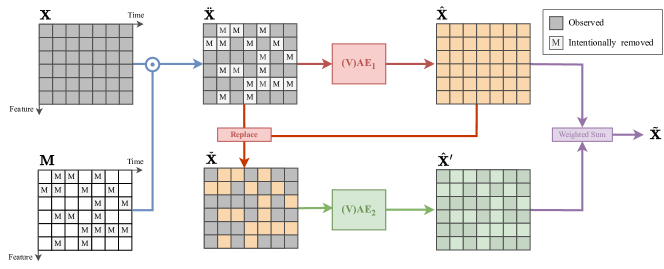
Figure 4. Overall workflow of our proposed dual-layer imputation method. We intentionally remove some elements in $\ddot{\mathbf{X}}$ for the training effect in challenging environments.

4.3. Output Layer

In order to infer an observation $\hat{\mathbf{x}}_{i}$ at time $t_{i}$, we use the following output layer:

(13) $$\hat{\mathbf{x}}_{i}=\texttt{FC}_{2}(\texttt{ELU}(\texttt{FC}_{1}(\boldsymbol{d}(t_{i})))),$$

where FC means an fully-connected layer, and ELU means an exponential linear unit. Taking the elements of $\hat{\mathbf{x}}_{i}$ whose original values are nan in $\mathbf{x}_{i}$, we can accomplish the time series imputation task.

4.4. Augmented ODE for Encoder and Decoder

In order to implement our model, we use the following augmented ordinary differential equation (ODE):

(14) $$\frac{d}{dt}{\begin{bmatrix}\boldsymbol{\mu}(t)\\ \boldsymbol{\sigma}(t)\\ \boldsymbol{d}(t)\\ \end{bmatrix}\!}={\begin{bmatrix}g_{\mu}(\boldsymbol{e}(t),t;\boldsymbol{\theta}_{\mu})\frac{dX(t)}{dt}\\ g_{\sigma}(\boldsymbol{e}(t),t;\boldsymbol{\theta}_{\sigma})\frac{dX(t)}{dt}\\ k(\boldsymbol{d}(t);\boldsymbol{\theta}_{k})\Big{(}\frac{d\boldsymbol{\mu}(t)}{dt}+\boldsymbol{\epsilon}_{t}\odot\frac{d\exp(\boldsymbol{\sigma}(t))}{dt}\Big{)}\\ \end{bmatrix}.\!}$$

and

$${\begin{bmatrix}\boldsymbol{\mu}(0)\\ \boldsymbol{\sigma}(0)\\ \boldsymbol{d}(0)\\ \end{bmatrix}\!}={\begin{bmatrix}\texttt{FC}_{\mu}(X(0))\\ \texttt{FC}_{\sigma}(X(0))\\ \texttt{FC}_{\boldsymbol{d}}(X(0))\\ \end{bmatrix}.\!}$$

Throughout Eq. (14), we can integrate our proposed continuous-time encoder and decode into a single ODE state, which means that by solving the ODE, the entire forward pass of our continuous-time variational autoencoder can be calculated simultaneously.

Why continuous hidden path?:

We note that the hidden representation $H(t)$ in Eq. (6) is continuously defined over time, which is different from existing methods where only a single hidden representation is created after reading the entire time series (cf. Fig. 1(a) vs. 1(b)). The benefits of our proposed continuous hidden path are two folds.

Firstly, our proposed method is suitable for time series imputation. For instance, suppose that we want to infer $(\hat{\mathbf{x}}_{j},t_{j})$ for time series imputation. $H(t_{j})$ contains the information of the input time series up to time $t$ and its near future — note that additional information around time point $t_{j}$ is used when creating $X(t_{j})$ with an interpolation method (cf. Fig 3). Thus, $H(t_{j})$ contains enough information to infer $\hat{\mathbf{x}}_{j}$ via the decoder and the output layer.

Secondly, our proposed method provides one-way lightweight processing. Only by solving the augmented ODE in Eq. (14) from an initial time $0$ to a terminal time $T$ sequentially and incrementally, we can impute all missing elements with the output layer.

Vanilla autoencoder:

Our framework can be converted to the vanilla autoencoder in a naïve way only by i) setting $H(t)=\boldsymbol{\mu}(t)$ after removing $\boldsymbol{\sigma}(t)$ and ii) using the usual reconstruction loss (without the ELBO (Kingma and Welling, 2013) loss). Since we discard $\boldsymbol{\sigma}(t)$ in this vanilla setting, its inference time and space complexities are reduced in comparison with those of the variational autoencoder setting.

How to infer:

For inference, we use only $\boldsymbol{\mu}(t)$, i.e., $H(t)=\boldsymbol{\mu}(t)$ is used for the variational autoencoder setting. In other words, we use the mean hidden representation only. By considering $\boldsymbol{\sigma}(t)$, we can further extract the confidence interval, but our main interest is how to impute incomplete time series. For the vanilla setting, we remove $\boldsymbol{\sigma}(t)$ so it clear that $H(t)=\boldsymbol{\mu}(t)$ for inference.

4.5. Dual Autoencoder Architecture

We have described how a single (variational) autoencoder can be defined so far. For time series imputation, however, two-layer architectures are popular (Du et al., 2023). We also propose the following dual-autoencoder approach and its training method (cf. Fig. 4):

1. (Blue Path of Fig. 4) Given a training time series sample $\mathbf{X}$, i.e., a matrix representation of $\{(\mathbf{x}_{i},t_{i})\}_{i=0}^{N}$, we intentionally remove some more elements from $\mathbf{X}$ in order to create more challenging training environments. The intentionally removed elements are marked as ‘M’ in Fig. 4, and we use $\mathbf{M}$ to denote the masking matrix, e.g., 1 in $\mathbf{M}$ means ‘intentionally removed by us.’ We use $N_{M}$ to denote the number of these intentionally removed elements, which is a hyperparameter for our training method.

2. (Red Path of Fig. 4) We first take $\hat{\mathbf{X}}$, i.e., $\{(\hat{\mathbf{x}}_{t_{i}},t_{i})\}_{i=0}^{N}$, from the initial proposed (variational) autoencoder marked as ‘$(V)AE_{1}$’ in Fig. 4. We then create the initial imputation outcome $\check{\mathbf{X}}$ by replacing the missing nan elements of $\ddot{\mathbf{x}}_{t_{i}}$ with the inferred elements of $\hat{\mathbf{x}}_{t_{i}}$ for all $i$.

3. (Green Path of Fig. 4) We then feed $\check{\mathbf{X}}$ to the next proposed (variational) autoencoder. Let $\hat{\mathbf{X}}^{\prime}$, i.e., $\{(\hat{\mathbf{x}}^{\prime}_{i},t_{i})\}_{i=0}^{N}$, be the output from the second autoendoer via the residual connection with $\check{\mathbf{X}}$.

4. (Purple Path of Fig. 4) We then let $\tilde{\mathbf{X}}$, i.e., $\{(\tilde{\mathbf{x}}_{j},t_{j})\}_{i=0}^{N}$, be our final imputation outcome, which is calculated as follows — in other words, the first and second imputation outcomes are connected through the learnable weighted sum:

   (15) $$\tilde{\mathbf{x}}_{j}=\boldsymbol{\alpha}\odot\hat{\mathbf{x}}_{j}+(\mathbf{1}-\boldsymbol{\alpha})\odot\hat{\mathbf{x}}^{\prime}_{j},$$

   where $\boldsymbol{\alpha}=\phi(\texttt{FC}_{3}(\boldsymbol{d}^{\prime}(t_{j})))$, $\phi$ is Sigmoid, and $\boldsymbol{d}^{\prime}(t_{j})$ means the hidden representation of the decoder of the 2nd autoencoder at time $t_{j}$. $\odot$ means the element-wise multiplication.

Input: Training data $D_{train}$, Validating data $D_{val}$, Maximum iteration numbers $max\_iter$

1 Initialize the model parameter $\Theta$ which includes $\boldsymbol{\theta}_{\mu},\boldsymbol{\theta}_{\sigma},\boldsymbol{\theta}_{k}$ and additional parameters for other layers;

2

3$i\leftarrow 0$;

4while $i<max\_iter$ do

5       Create a mini-batch $B:=\{(\mathbf{X}_{b},\ddot{\mathbf{X}}_{b})\}_{b=1}^{N_{B}}$;

6       Train $\Theta$ using the loss $L$ with $B$;

7       Validate and update the best parameter $\Theta$ with $D_{val}$;

8      

9      $i\leftarrow i+1$;

return $\Theta$;

Algorithm 1 How to train CTA

Training method:

In order to train the dual autoencoders, we use the following loss function and the method in Alg. 1:

(16) $$\begin{split}L:=&\overset{\textrm{Reconstruction}}{\overbrace{||(\mathbf{X}-\tilde{\mathbf{X}})||_{F}+||(\mathbf{X}-\hat{\mathbf{X}})||_{F}+||(\mathbf{X}-\hat{\mathbf{X}}^{\prime})||_{F}+||\mathbf{M}\odot(\mathbf{X}-\tilde{\mathbf{X}})||_{F}}}\\ &+\overset{\textrm{KL Divergence}}{\overbrace{\int_{0}^{T}KLD_{1}(t)+KLD_{2}(t)dt}},\end{split}$$

where we use $KLD_{1}(t)$ and $KLD_{2}(t)$ for brevity to denote the usual KL divergence (Csiszár, 1975) terms of the first and the second variational autoencoders at time $t$, respectively — note that those KL Divergence terms can be omitted for the vanilla setting of our proposed method. In particular, those KLD terms can be defined for every time point $t$ since our CTA is a method to create an infinite number of variational autoencoders in $[0,T]$ (cf. Fig. 2) and therefore, we need to integrate them over time. We use existing ODE solvers for this purpose as we do it for NCDEs (see Appendix 4.5 for details). We also note that our loss is a continuous generalization of the ELBO loss since we have an infinite number of variational autoencoders in the time domain $[0,T]$ and therefore, the KLD loss term is defined for every time point $t\in[0,T]$.

In Alg. 1, we first initialize all the model parameters, denoted $\Theta$. In Line 1, we create a mini-batch of size $N_{B}$. Each pair of $(\mathbf{X}_{b},\ddot{\mathbf{X}}_{b})$ means an incomplete time series sample $\ddot{\mathbf{X}}_{b}$ and its ground-truth sample $\mathbf{X}_{b}$. In Line 1, we train $\Theta$ following the method described for Fig. 4. As described, our training process intentionally removes $N_{M}$ more elements from each $\ddot{\mathbf{X}}_{b}$ to increase the effect of the supervised training. Our CTA produces two intermediate and one final inference outcomes, i.e., $\tilde{\mathbf{X}}_{b},\hat{\mathbf{X}}_{b}$, and $\hat{\mathbf{X}}^{\prime}_{b}$, for each training sample $\ddot{\mathbf{X}}_{b}$, with which the training with the loss $L$ is conducted.

Role of each layer:

In the proposed dual autoencoder architecture, the first (variational) autoencoder infers the initial imputed time series where for some challenging imputation points, its quality may not be satisfactory. The second (variational) autoencoder then tries to complement for the challenging cases via the learnable weighted sum, i.e., the learnable residual connection. In ablation study, we analyze the benefits of the dual-layer architecture.

How to Solve $\int_{0}^{T}KLD(t)dt$?:

Our loss function in Eq. (16) requires an integral problem to calculate the KLD terms along the time in $[0,T]$. For simplicity but without loss of generality, we assume only one variational autoencoder so we need to solve $\int_{0}^{T}KLD(t)dt$. For this, we define and solve the following augmented ODE to calculate all the hidden states and the KLD loss at the same time. Therefore, $\xi(T)$ corresponds to the Riemann integral of $\int_{0}^{T}KLD(t)dt$ and contains the final KLD loss value.

$$\frac{d}{dt}{\begin{bmatrix}\boldsymbol{\mu}(t)\\ \boldsymbol{\sigma}(t)\\ \boldsymbol{d}(t)\\ \xi(t)\end{bmatrix}\!}={\begin{bmatrix}g_{\mu}(\boldsymbol{e}(t),t;\boldsymbol{\theta}_{\mu})\frac{dX(t)}{dt}\\ g_{\sigma}(\boldsymbol{e}(t),t;\boldsymbol{\theta}_{\sigma})\frac{dX(t)}{dt}\\ k(\boldsymbol{d}(t);\boldsymbol{\theta}_{k})\Big{(}\frac{d\boldsymbol{\mu}(t)}{dt}+\boldsymbol{\epsilon}_{t}\odot\frac{d\exp(\boldsymbol{\sigma}(t))}{dt}\Big{)}\\ KLD(t)\end{bmatrix}.\!}$$

Table 2. Performance on AirQuality and Stocks. The best results are in boldface and the second best results are underlined. Lower errors are preferred. SA-based$(^{\ast})$ indicates self-attention-based model.

Dataset		AirQuality						Stocks
		30%		50%		70%		30%		50%		70%
		MAE	RMSE	MAE	RMSE	MAE	RMSE	MAE	RMSE	MAE	RMSE	MAE	RMSE
Statistical	KNN	0.328±0.001	0.621±0.018	0.352±0.000	0.673±0.014	0.503±0.000	0.859±0.005	0.614±0.061	2.081±0.218	0.612±0.046	1.963±0.175	0.754±0.013	2.066±0.116
	MICE	2.377±0.010	6.073±0.030	0.494±0.004	1.110±0.016	0.335±0.000	0.654±0.007	0.755±0.080	2.254±0.224	0.752±0.035	2.091±0.138	0.990±0.015	2.243±0.110
RNN-based	GRU-D	0.459±0.016	0.740±0.020	0.466±0.014	0.761±0.017	0.482±0.013	0.780±0.016	0.868±0.009	2.222±0.003	0.735±0.005	1.743±0.005	0.936±0.012	2.015±0.005
	ODE-RNN	0.370±0.000	0.611±0.000	0.371±0.000	0.632±0.000	0.383±0.000	0.650±0.000	0.740±0.000	1.919±0.000	0.718±0.000	1.720±0.000	0.857±0.000	1.873±0.000
	MRNN	0.309±0.001	0.566±0.019	0.325±0.000	0.585±0.014	0.352±0.000	0.614±0.006	0.789±0.062	2.170±0.217	0.745±0.041	2.101±0.168	0.766±0.020	2.086±0.118
	BRITS	0.212±0.001	0.470±0.015	0.231±0.000	0.494±0.013	0.253±0.000	0.527±0.007	0.413±0.048	1.635±0.210	0.462±0.042	1.651±0.182	0.600±0.023	1.966±0.126
VAE-based	RNN-VAE	0.704±0.000	1.009±0.001	0.704±0.001	1.019±0.001	0.702±0.000	1.016±0.000	1.576±0.011	2.529±0.032	1.427±0.008	2.173±0.031	1.509±0.003	2.274±0.005
	LatentODE	0.466±0.000	0.723±0.000	0.453±0.001	0.732±0.001	0.464±0.000	0.739±0.000	0.562±0.003	1.802±0.005	0.461±0.002	1.515±0.006	0.534±0.001	1.636±0.002
	VRNN	0.450±0.001	0.744±0.016	0.510±0.001	0.803±0.011	0.584±0.000	0.880±0.004	1.047±0.061	2.284±0.214	1.152±0.044	2.197±0.166	1.404±0.021	2.396±0.109
	SRNN	0.366±0.001	0.632±0.019	0.460±0.001	0.734±0.012	0.560±0.000	0.846±0.005	0.782±0.055	1.984±0.214	1.063±0.043	2.102±0.169	1.364±0.022	2.367±0.110
	STORN	0.450±0.001	0.743±0.016	0.509±0.001	0.799±0.011	0.583±0.000	0.879±0.005	1.037±0.060	2.237±0.212	1.133±0.041	2.161±0.166	1.386±0.022	2.385±0.111
	GP-VAE	0.287±0.001	0.517±0.015	0.303±0.001	0.547±0.013	0.307±0.001	0.556±0.005	0.494±0.049	1.574±0.211	0.531±0.044	1.503±0.194	0.560±0.029	1.604±0.216
GAN-based	GRUI-GAN	0.851±0.003	1.165±0.010	0.843±0.002	1.154±0.008	0.820±0.002	1.128±0.005	0.766±0.060	2.035±0.209	1.307±0.066	2.342±0.179	1.845±0.020	2.620±0.100
	E2GAN	0.742±0.001	1.056±0.012	0.746±0.001	1.060±0.009	0.747±0.001	1.074±0.004	1.556±0.050	2.641±0.176	1.533±0.040	2.430±0.150	1.511±0.023	2.468±0.106
	GAIN	0.440±0.001	0.680±0.014	0.555±0.000	0.808±0.011	0.657±0.000	0.938±0.005	1.127±0.057	2.267±0.205	1.187±0.048	2.147±0.166	1.421±0.013	2.442±0.094
SA-based(∗)	mTAN	0.257±0.000	0.497±0.002	0.273±0.000	0.518±0.007	0.289±0.000	0.556±0.002	0.390±0.005	1.045±0.020	0.345±0.006	1.082±0.013	0.497±0.016	1.576±0.012
	HetVAE	0.243±0.000	0.505±0.021	0.251±0.000	0.518±0.016	0.281±0.000	0.557±0.006	0.319±0.046	1.345±0.229	0.384±0.037	1.500±0.176	0.421±0.024	1.612±0.146
	Transformer	0.222±0.000	0.475±0.017	0.235±0.001	0.494±0.013	0.254±0.000	0.523±0.008	0.388±0.047	1.476±0.230	0.378±0.036	1.402±0.186	0.489±0.024	1.764±0.131
	SAITS	0.201±0.000	0.449±0.016	0.230±0.001	0.493±0.012	0.247±0.000	0.513±0.006	0.374±0.048	1.461±0.233	0.371±0.036	1.369±0.195	0.474±0.026	1.733±0.129
CTA (ours)	VAE-AE	0.186±0.000	0.424±0.023	0.202±0.000	0.447±0.019	0.237±0.000	0.513±0.007	0.289±0.034	1.138±0.186	0.281±0.035	1.075±0.191	0.335±0.008	1.283±0.107
	AE-AE	0.200±0.001	0.438±0.020	0.217±0.000	0.481±0.018	0.235±0.000	0.508±0.008	0.300±0.035	1.204±0.160	0.315±0.020	1.202±0.108	0.364±0.009	1.365±0.074

Original Missing Elements of  $\mathbf{X}$:

For ease of our discussion, we assumed that for $\mathbf{X}$, all ground-truth elements are known in the main body of this paper. In our experiments, however, some ground-truth elements are unknown in their originally released dataset. In this situation, we cannot use those elements for training and testing. Modifying our descriptions in the main paper to consider those missing ground-truth elements is straightforward. For instance, $\boldsymbol{\alpha}$ is redefined to $\boldsymbol{\alpha}=\phi(\texttt{FC}_{3}(\boldsymbol{d}^{\prime}(t_{j}),\mathbf{O}))$ and the loss function can be rewritten as follows:

$$\begin{split}L:=&\overset{\textrm{Reconstruction}}{\overbrace{||\mathbf{O}\odot(\mathbf{X}-\tilde{\mathbf{X}})||_{F}+||\mathbf{O}\odot(\mathbf{X}-\hat{\mathbf{X}})||_{F}+||\mathbf{O}\odot(\mathbf{X}-\hat{\mathbf{X}}^{\prime})||_{F}}}\\ &+\overset{\textrm{Reconstruction}}{\overbrace{||\mathbf{M}\odot(\mathbf{X}-\tilde{\mathbf{X}})||_{F}}}+\overset{\textrm{KL Divergence}}{\overbrace{\int_{0}^{T}KLD_{1}(t)+KLD_{2}(t)dt}},\end{split}$$

where $\mathbf{O}$ means a masking matrix to denote those elements whose ground-truth values are known in its original dataset.

Table 3. Performance on Electricity and Energy. The best results are in boldface and the second best results are underlined. Lower errors are preferred. SA-based$(^{\ast})$ indicates self-attention-based model.

Dataset		Electricity						Energy
		30%		50%		70%		30%		50%		70%
		MAE	RMSE	MAE	RMSE	MAE	RMSE	MAE	RMSE	MAE	RMSE	MAE	RMSE
Statistical	KNN	1.369±0.000	2.047±0.002	1.356±0.000	2.060±0.001	1.421±0.000	2.137±0.001	0.583±0.006	0.787±0.009	0.819±0.003	1.071±0.005	1.109±0.005	1.404±0.005
	MICE	0.867±0.000	1.398±0.001	0.906±0.000	1.559±0.001	0.972±0.000	1.662±0.001	0.513±0.005	0.761±0.009	0.543±0.003	0.743±0.004	0.829±0.003	1.075±0.005
RNN-based	GRU-D	1.564±0.003	2.180±0.004	1.586±0.005	2.200±0.008	1.612±0.005	2.211±0.007	0.537±0.009	0.713±0.010	0.544±0.010	0.727±0.012	0.562±0.009	0.755±0.012
	ODE-RNN	1.539±0.000	2.169±0.000	1.529±0.000	2.150±0.000	1.519±0.000	2.137±0.000	0.517±0.000	0.698±0.000	0.541±0.000	0.728±0.000	0.574±0.000	0.767±0.000
	MRNN	1.272±0.000	1.900±0.002	1.297±0.000	1.925±0.001	1.325±0.000	1.944±0.001	0.555±0.003	0.736±0.006	0.593±0.002	0.781±0.005	0.654±0.002	0.842±0.003
	BRITS	0.915±0.000	1.510±0.002	0.980±0.000	1.602±0.001	1.110±0.000	1.737±0.001	0.172±0.004	0.324±0.011	0.278±0.004	0.438±0.009	0.411±0.001	0.589±0.005
VAE-based	RNN-VAE	1.864±0.000	2.447±0.000	1.849±0.000	2.413±0.000	1.846±0.000	2.417±0.000	0.965±0.001	1.211±0.000	0.973±0.000	1.220±0.001	0.968±0.000	1.213±0.000
	LatentODE	1.814±0.001	2.450±0.001	1.732±0.001	2.352±0.001	1.777±0.001	2.404±0.001	0.712±0.002	0.935±0.003	0.697±0.008	0.912±0.009	0.698±0.008	0.916±0.009
	VRNN	1.565±0.000	2.159±0.002	1.635±0.000	2.224±0.001	1.705±0.000	2.281±0.001	0.896±0.004	1.141±0.004	0.920±0.001	1.161±0.003	0.933±0.001	1.172±0.002
	SRNN	1.534±0.000	2.063±0.001	1.636±0.000	2.185±0.001	1.700±0.000	2.256±0.001	0.537±0.004	0.717±0.007	0.654±0.002	0.846±0.005	0.783±0.001	0.995±0.003
	STORN	1.532±0.000	2.098±0.001	1.622±0.000	2.188±0.001	1.702±0.000	2.265±0.001	0.869±0.005	1.100±0.006	0.895±0.002	1.132±0.003	0.915±0.001	1.152±0.002
	GP-VAE	1.006±0.000	1.633±0.001	1.058±0.000	1.704±0.001	1.119±0.000	1.764±0.001	0.407±0.001	0.551±0.004	0.496±0.003	0.654±0.006	0.504±0.001	0.668±0.002
GAN-based	GRUI-GAN	1.919±0.001	2.510±0.002	1.905±0.001	2.508±0.002	1.894±0.001	2.487±0.001	0.958±0.004	1.171±0.005	1.057±0.007	1.329±0.006	0.999±0.005	1.262±0.007
	E2GAN	1.883±0.000	2.459±0.001	1.874±0.000	2.442±0.001	1.880±0.000	2.457±0.001	0.856±0.005	1.088±0.003	0.843±0.002	1.066±0.002	0.864±0.002	1.103±0.003
	GAIN	1.304±0.000	1.832±0.001	1.546±0.000	2.109±0.001	1.733±0.000	2.288±0.001	0.647±0.004	0.842±0.006	0.811±0.001	1.033±0.004	0.917±0.002	1.148±0.004
SA-based(∗)	mTAN	1.326±0.000	1.840±0.000	1.378±0.000	1.887±0.000	1.386±0.000	1.962±0.000	0.394±0.001	0.553±0.001	0.389±0.001	0.549±0.001	0.422±0.000	0.595±0.000
	HetVAE	1.168±0.001	1.973±0.002	1.238±0.000	1.878±0.001	1.176±0.000	1.850±0.001	0.316±0.004	0.486±0.008	0.335±0.002	0.501±0.003	0.409±0.002	0.589±0.006
	Transformer	0.899±0.000	1.336±0.001	0.946±0.000	1.518±0.001	0.988±0.000	1.574±0.001	0.347±0.005	0.515±0.014	0.423±0.004	0.601±0.008	0.502±0.003	0.705±0.006
	SAITS	0.894±0.000	1.404±0.001	0.953±0.000	1.581±0.001	1.024±0.000	1.680±0.001	0.313±0.006	0.484±0.015	0.392±0.004	0.570±0.008	0.484±0.004	0.675±0.007
CTA (ours)	VAE-AE	0.767±0.000	1.127±0.001	0.748±0.000	1.146±0.001	0.781±0.000	1.149±0.001	0.205±0.004	0.343±0.011	0.227±0.001	0.381±0.006	0.287±0.002	0.460±0.007
	AE-AE	0.742±0.000	1.139±0.001	0.772±0.000	1.162±0.001	0.810±0.000	1.215±0.001	0.170±0.004	0.316±0.014	0.208±0.002	0.365±0.007	0.280±0.002	0.450±0.007

5. Experiments

In this section, we describe our experimental environments followed by experimental results and analyses.

5.1. Experimental Environments

5.1.1. Datasets

To evaluate the performance of various methods, we use four real-world datasets from different domains as follows: AirQuality, Stocks, Electricity and Energy (See supplementray material for their details).

5.1.2. Baselines

We compare our method with 19 baselines, which include statistical methods, VAE-based, RNN-based, GAN-based and self-attention-based methods (see supplementray material for details).

5.1.3. Evaluation Methods

To evaluate our method and baselines, we utilize two metrics: MAE (Mean Absolute Error) and RMSE (Root Mean Square Error). These are commonly used in the time series imputation literature (Cao et al., 2018; Du et al., 2023; Shukla and Marlin, 2021). We report the mean and standard deviation of the error for five trials.

In order to create more challenging evaluation environments, we increase the percentage of the missing elements, denoted $r_{missing}$. We remove the element by the ratio of $r_{missing}$ from the training, i.e., the model does not learn about this missing elements, and test datasets, i.e., the imputation task’s targets are those missing elements. In total, we test in three different settings, i.e., $r_{missing}\in\{30\%,50\%,70\%\}$. The above evaluation metrics are measured only for those missing elements since our task is imputation.

5.1.4. Hyperparameters

We report the search range of each hyperparameter in our method and all the baselines in our supplementary material. In addition, we summarize the best hyperparameter of our method for reproducibility in the supplementray material.

5.2. Experimental Results

Table 2 summarizes the results on AirQuality and Stocks. For AirQuality, the performances of SAITS and BRITS are the best among the baselines for all missing rates, but CTA shows the lowest errors in all cases.

In the case of Stocks, our method, the self-attention-based methods, and some of the VAE-based methods work reasonably. When $r_{missing}$ is 30%, mTAN performs slightly better than our model in RMSE. However, in all other cases, the performance of CTA (VAE-AE) outperforms other baselines by large margins.

The results on Electricity and Energy are shown in Table 3. For Electricity, MICE, which is a statistical method, shows the best result among all the baselines. However, Our CTA marks the best accuracy in general. In particular, CTA significantly outperforms others baselines when $r_{missing}$ is high.

In the case of Energy, BRITS shows the best performance among the baselines. However, it is shown that the error increases rapidly as $r_{missing}$ increases. When $r_{missing}$ is high, the performance of HetVAE is the best among the baselines, but our CTA (AE-AE) outperforms other baselines at all missing rates.

Table 4. The number of model parameters and the GPU memory usage for the best hyperparameter settings of CTA and SAITS with $r_{missing}$=70%

	SAITS	CTA
AirQuality	2.35 M / 204.33 MB	1.52 M / 57.45 MB (AE-AE)
Stocks	12.64 M / 184.89 MB	0.02 M / 0.42 MB (VAE-AE)
Electricity	16.13 M / 1,185.44 MB	53.26 M / 950.85 MB (VAE-AE)
Energy	11.64 M / 443.85 MB	0.92 M / 13.41 MB (AE-AE)

5.3. Empirical Complexity

We compare the model sizes and the inference GPU memory usage of our method and SAITS, the best-performing baseline, in Table 4. Except for the number of parameters for Electricity, our model has a smaller size and consumes less GPU memory than SAITS. Especially for Stocks and Energy, our model’s size is 2 to 3 orders of magnitude smaller than that of SAITS, which is an outstanding result. One more interesting point is that for Electricity, CTA marks comparable GPU memory footprint to SAITS with more parameters, which shows the efficiency of our computation.

Table 5. Results with various architectures for our CTA on AirQuality and Stocks with $r_{missing}$=70%. The best results are in boldface and the second best results are underlined.

	AirQuality		Stocks
	MAE	RMSE	MAE	RMSE
AE	0.240±0.000	0.513±0.008	0.655±0.182	3.369±1.122
VAE	0.246±0.000	0.520±0.007	0.370±0.043	1.432±0.117
AE-AE (ours)	0.235±0.000	0.508±0.008	0.364±0.009	1.365±0.074
AE-VAE	0.252±0.001	0.523±0.007	0.456±0.068	1.711±0.192
VAE-AE (ours)	0.237±0.000	0.513±0.007	0.335±0.008	1.283±0.107
VAE-VAE	0.238±0.000	0.514±0.008	0.406±0.041	1.584±0.171
AE-AE-AE	0.235±0.000	0.504±0.005	0.509±0.096	2.013±0.426
AE-AE-VAE	0.236±0.000	0.503±0.007	0.385±0.007	1.410±0.122
AE-VAE-AE	0.236±0.000	0.507±0.008	0.370±0.010	1.391±0.097
AE-VAE-VAE	0.237±0.000	0.509±0.007	0.358±0.011	1.366±0.109
VAE-AE-AE	0.237±0.000	0.504±0.008	0.389±0.011	1.404±0.105
VAE-AE-VAE	0.237±0.000	0.505±0.008	0.409±0.011	1.414±0.085
VAE-VAE-AE	0.238±0.000	0.511±0.007	0.465±0.049	1.743±0.195
VAE-VAE-VAE	0.238±0.000	0.512±0.007	0.404±0.013	1.448±0.115

5.4. Ablation Study on Dual-Layer Architecture

Since CTA uses a dual-layer autoencoder architecture, we conduct an ablation study by varying the number of layers. We test all the combinations from single to triple layers, and their results are shown in Table 5 for AirQuality and Stocks with the 70% missing rate. In general, VAE-AE and AE-AE show good results for our CTA. In both datasets, the single-layer ablation models, i.e., AE and VAE, produce worse outcomes than those of the dual-layer models. Among the dual-layer models, it shows better outcomes when the second layer is AE instead of VAE. For AirQuality, The performances of dual and triple-layer are not significantly different.

Table 6. Results with the interpolation method on AirQuality and Stocks with $r_{missing}$=70%. The best results are in boldface.

	AirQuality		Stocks
	MAE	RMSE	MAE	RMSE
Natural Cubic Spline	0.250±0.001	0.658±0.052	0.412±0.031	1.704±0.157
CTA(VAE-AE)	0.237±0.000	0.513±0.007	0.335±0.008	1.283±0.107
CTA(AE-AE)	0.235±0.000	0.508±0.008	0.364±0.009	1.365±0.074

5.5. Comparison to Interpolation method

We use the natural cubic spline method to build $X(t)$. We report the performance of the interpolation itself in the extreme case of the 70% missing rate in AirQuality and Stocks. As shown in Table 6, it can be observed that the performance is improved compared to the interpolation alone.

6. Conclusion

In this paper, we tackled how to impute regular and irregular time series. We presented a novel method based on NCDEs, which generalizes (variational) autoencoders in a continuous manner. Our method creates one (variational) autoencoder every time point and therefore, there are an infinite number of (variational) autoencoders along the time domain $[0,T]$. For this, the ELBO loss is calculated after solving an integral problem. Therefore, training occurs for every time point in the time domain, which drastically increases the training efficacy. We also presented a dual-layered architecture.

In our experiments with 4 datasets and 19 baselines, our presented method clearly marks the best accuracy in all cases. Moreover, our models have much smaller numbers of parameters than those of the state-of-the-art method. Our ablation and sensitivity studies also justify our method design. SAITS also has a dual-transformer architecture. Therefore, the main difference between our method and SAITS is that our method continuously generalizes (variational) autoencoders.

In the future, our method can be adopted to solving other time series tasks, such as classification and forecasting. Time series synthesis (Yoon et al., 2019; Jeon et al., 2022) is also one more application to which our method can be applied.

Ethical Consideration

Our model focuses on advancing the time series imputation. While our model itself hasn’t introduced any new ethical issues, it brings to light potential concerns regarding privacy and anonymity. As data is harnessed for imputation, it’s crucial to thoughtfully address the ethical considerations surrounding the confidentiality of sensitive information and the preservation of individual anonymity. balancing between data utility and safeguarding personal privacy will be crucial in ensuring the responsible and trustworthy deployment of our model. As we continue to improve and implement our model, we are committed to maintaining the highest standards of ethics and privacy, and to promoting discussions on integrating solutions that acknowledge these concerns and prioritize the well-being of all stakeholders involved.

- (1)
- Bayer and Osendorfer (2014) Justin Bayer and Christian Osendorfer. 2014. Learning stochastic recurrent networks. arXiv preprint arXiv:1411.7610 (2014).
- Cao et al. (2018) Wei Cao, Dong Wang, Jian Li, Hao Zhou, Lei Li, and Yitan Li. 2018. Brits: Bidirectional recurrent imputation for time series. Advances in neural information processing systems 31 (2018).
- Che et al. (2018) Zhengping Che, Sanjay Purushotham, Kyunghyun Cho, David Sontag, and Yan Liu. 2018. Recurrent neural networks for multivariate time series with missing values. Scientific reports 8, 1 (2018), 1–12.
- Chen et al. (2001) Chao Chen, Karl Petty, Alexander Skabardonis, Pravin Varaiya, and Zhanfeng Jia. 2001. Freeway performance measurement system: mining loop detector data. Transportation Research Record 1748, 1 (2001), 96–102.
- Chen et al. (2018) Ricky TQ Chen, Yulia Rubanova, Jesse Bettencourt, and David K Duvenaud. 2018. Neural ordinary differential equations. Advances in neural information processing systems 31 (2018).
- Cho et al. (2014) Kyunghyun Cho, Bart Van Merriënboer, Caglar Gulcehre, Dzmitry Bahdanau, Fethi Bougares, Holger Schwenk, and Yoshua Bengio. 2014. Learning phrase representations using RNN encoder-decoder for statistical machine translation. arXiv preprint arXiv:1406.1078 (2014).
- Choi et al. (2023) Hwangyong Choi, Jeongwhan Choi, Jeehyun Hwang, Kookjin Lee, Dongeun Lee, and Noseong Park. 2023. Climate Modeling with Neural Advection–Diffusion Equation. Knowledge and Information Systems (2023).
- Choi et al. (2022) Jeongwhan Choi, Hwangyong Choi, Jeehyun Hwang, and Noseong Park. 2022. Graph Neural Controlled Differential Equations for Traffic Forecasting. In AAAI.
- Choi and Park (2023) Jeongwhan Choi and Noseong Park. 2023. Graph Neural Rough Differential Equations for Traffic Forecasting. ACM Transactions on Intelligent Systems and Technology (2023).
- Chung et al. (2015) Junyoung Chung, Kyle Kastner, Laurent Dinh, Kratarth Goel, Aaron C Courville, and Yoshua Bengio. 2015. A recurrent latent variable model for sequential data. Advances in neural information processing systems 28 (2015).
- Csiszár (1975) Imre Csiszár. 1975. I-divergence geometry of probability distributions and minimization problems. The annals of probability (1975), 146–158.
- Dingli and Fournier (2017) Alexiei Dingli and Karl Sant Fournier. 2017. Financial time series forecasting-a deep learning approach. International Journal of Machine Learning and Computing 7, 5 (2017), 118–122.
- Du et al. (2023) Wenjie Du, David Côté, and Yan Liu. 2023. Saits: Self-attention-based imputation for time series. Expert Systems with Applications 219 (2023), 119619.
- Elfwing et al. (2018) Stefan Elfwing, Eiji Uchibe, and Kenji Doya. 2018. Sigmoid-weighted linear units for neural network function approximation in reinforcement learning. Neural Networks 107 (2018), 3–11.
- Fang et al. (2021) Zheng Fang, Qingqing Long, Guojie Song, and Kunqing Xie. 2021. Spatial-temporal graph ode networks for traffic flow forecasting. In Proceedings of the 27th ACM SIGKDD conference on knowledge discovery & data mining. 364–373.
- Fortuin et al. (2020) Vincent Fortuin, Dmitry Baranchuk, Gunnar Rätsch, and Stephan Mandt. 2020. Gp-vae: Deep probabilistic time series imputation. In AISTATS.
- Fraccaro et al. (2016) Marco Fraccaro, Søren Kaae Sønderby, Ulrich Paquet, and Ole Winther. 2016. Sequential neural models with stochastic layers. Advances in neural information processing systems 29 (2016).
- Girin et al. (2021) Laurent Girin, Simon Leglaive, Xiaoyu Bie, Julien Diard, Thomas Hueber, and Xavier Alameda-Pineda. 2021. Dynamical Variational Autoencoders: A Comprehensive Review. Foundations and Trends® in Machine Learning 15, 1-2 (2021), 1–175. https://doi.org/10.1561/2200000089
- Hewage et al. (2020) Pradeep Hewage, Ardhendu Behera, Marcello Trovati, Ella Pereira, Morteza Ghahremani, Francesco Palmieri, and Yonghuai Liu. 2020. Temporal convolutional neural (TCN) network for an effective weather forecasting using time-series data from the local weather station. Soft Computing 24 (2020), 16453–16482.
- Hochreiter and Schmidhuber (1997) Sepp Hochreiter and Jürgen Schmidhuber. 1997. Long short-term memory. Neural computation 9, 8 (1997), 1735–1780.
- Hwang et al. (2021) Jeehyun Hwang, Jeongwhan Choi, Hwangyong Choi, Kookjin Lee, Dongeun Lee, and Noseong Park. 2021. Climate Modeling with Neural Diffusion Equations. In ICDM. 230–239.
- Jeon et al. (2022) Jinsung Jeon, Jeonghak Kim, Haryong Song, Seunghyeon Cho, and Noseong Park. 2022. GT-GAN: General Purpose Time Series Synthesis with Generative Adversarial Networks. In Advances in Neural Information Processing Systems.
- Jiang (2021) Weiwei Jiang. 2021. Applications of deep learning in stock market prediction: recent progress. Expert Systems with Applications 184 (2021), 115537.
- Jiang and Luo (2022) Weiwei Jiang and Jiayun Luo. 2022. Graph neural network for traffic forecasting: A survey. Expert Systems with Applications 207 (2022).
- Karevan and Suykens (2020) Zahra Karevan and Johan AK Suykens. 2020. Transductive LSTM for time-series prediction: An application to weather forecasting. Neural Networks 125 (2020), 1–9.
- Khare et al. (2017) Kaustubh Khare, Omkar Darekar, Prafull Gupta, and VZ Attar. 2017. Short term stock price prediction using deep learning. In 2017 2nd IEEE international conference on recent trends in electronics, information & communication technology (RTEICT). IEEE, 482–486.
- Kidger et al. (2020) Patrick Kidger, James Morrill, James Foster, and Terry Lyons. 2020. Neural controlled differential equations for irregular time series. Advances in neural information processing systems 33 (2020), 6696–6707.
- Kingma and Welling (2013) Diederik P Kingma and Max Welling. 2013. Auto-encoding variational bayes. arXiv preprint arXiv:1312.6114 (2013).
- Li and Zhu (2021) Mengzhang Li and Zhanxing Zhu. 2021. Spatial-temporal fusion graph neural networks for traffic flow forecasting. In Proceedings of the AAAI conference on artificial intelligence, Vol. 35. 4189–4196.
- Luo et al. (2018) Yonghong Luo, Xiangrui Cai, Ying Zhang, Jun Xu, et al. 2018. Multivariate time series imputation with generative adversarial networks. Advances in neural information processing systems 31 (2018).
- Luo et al. (2019) Yonghong Luo, Ying Zhang, Xiangrui Cai, and Xiaojie Yuan. 2019. E2gan: End-to-end generative adversarial network for multivariate time series imputation. In Proceedings of the 28th international joint conference on artificial intelligence. AAAI Press, 3094–3100.
- Ma et al. (2019) Jiawei Ma, Zheng Shou, Alireza Zareian, Hassan Mansour, Anthony Vetro, and Shih-Fu Chang. 2019. CDSA: cross-dimensional self-attention for multivariate, geo-tagged time series imputation. arXiv preprint arXiv:1905.09904 (2019).
- McKinley and Levine (1998) Sky McKinley and Megan Levine. 1998. Cubic spline interpolation. College of the Redwoods 45, 1 (1998), 1049–1060.
- Nazabal et al. (2020) Alfredo Nazabal, Pablo M Olmos, Zoubin Ghahramani, and Isabel Valera. 2020. Handling incomplete heterogeneous data using vaes. Pattern Recognition 107 (2020), 107501.
- Rubanova et al. (2019) Yulia Rubanova, Ricky TQ Chen, and David K Duvenaud. 2019. Latent ordinary differential equations for irregularly-sampled time series. Advances in neural information processing systems 32 (2019).
- Sen and Mehtab (2021) Jaydip Sen and Sidra Mehtab. 2021. Accurate stock price forecasting using robust and optimized deep learning models. In 2021 International Conference on Intelligent Technologies (CONIT). IEEE, 1–9.
- Shan et al. (2021) Siyuan Shan, Yang Li, and Junier B Oliva. 2021. Nrtsi: Non-recurrent time series imputation. arXiv preprint arXiv:2102.03340 (2021).
- Shi et al. (2015) Xingjian Shi, Zhourong Chen, Hao Wang, Dit-Yan Yeung, Wai-Kin Wong, and Wang-chun Woo. 2015. Convolutional LSTM network: A machine learning approach for precipitation nowcasting. Advances in neural information processing systems 28 (2015).
- Shukla and Marlin (2020) Satya Narayan Shukla and Benjamin Marlin. 2020. Multi-Time Attention Networks for Irregularly Sampled Time Series. In International Conference on Learning Representations.
- Shukla and Marlin (2021) Satya Narayan Shukla and Benjamin Marlin. 2021. Heteroscedastic Temporal Variational Autoencoder For Irregularly Sampled Time Series. In International Conference on Learning Representations.
- Silva et al. (2012) Ikaro Silva, George Moody, Daniel J Scott, Leo A Celi, and Roger G Mark. 2012. Predicting in-hospital mortality of icu patients: The physionet/computing in cardiology challenge 2012. In 2012 Computing in Cardiology. IEEE, 245–248.
- Stieltjes (1894) T-J Stieltjes. 1894. Recherches sur les fractions continues. In Annales de la Faculté des sciences de Toulouse: Mathématiques, Vol. 8. J1–J122.
- Suo et al. (2019) Qiuling Suo, Liuyi Yao, Guangxu Xun, Jianhui Sun, and Aidong Zhang. 2019. Recurrent imputation for multivariate time series with missing values. In 2019 IEEE international conference on healthcare informatics (ICHI). IEEE, 1–3.
- Tay et al. (2022) Yi Tay, Mostafa Dehghani, Dara Bahri, and Donald Metzler. 2022. Efficient Transformers: A Survey. ACM Comput. Surv. 55, 6 (2022).
- Tekin et al. (2021) Selim Furkan Tekin, Oguzhan Karaahmetoglu, Fatih Ilhan, Ismail Balaban, and Suleyman Serdar Kozat. 2021. Spatio-temporal weather forecasting and attention mechanism on convolutional lstms. arXiv preprint arXiv:2102.00696 (2021).
- Vargas et al. (2017) Manuel R Vargas, Beatriz SLP De Lima, and Alexandre G Evsukoff. 2017. Deep learning for stock market prediction from financial news articles. In 2017 IEEE international conference on computational intelligence and virtual environments for measurement systems and applications (CIVEMSA). IEEE, 60–65.
- Vaswani et al. (2017) Ashish Vaswani, Noam Shazeer, Niki Parmar, Jakob Uszkoreit, Llion Jones, Aidan N Gomez, Łukasz Kaiser, and Illia Polosukhin. 2017. Attention is all you need. Advances in neural information processing systems 30 (2017).
- Wu et al. (2019) Zonghan Wu, Shirui Pan, Guodong Long, Jing Jiang, and Chengqi Zhang. 2019. Graph wavenet for deep spatial-temporal graph modeling. arXiv preprint arXiv:1906.00121 (2019).
- Yoon et al. (2019) Jinsung Yoon, Daniel Jarrett, and Mihaela Van der Schaar. 2019. Time-series generative adversarial networks. Advances in neural information processing systems 32 (2019).
- Yoon et al. (2018a) Jinsung Yoon, James Jordon, and Mihaela Schaar. 2018a. Gain: Missing data imputation using generative adversarial nets. In International conference on machine learning. PMLR, 5689–5698.
- Yoon et al. (2018b) Jinsung Yoon, William R Zame, and Mihaela van der Schaar. 2018b. Estimating missing data in temporal data streams using multi-directional recurrent neural networks. IEEE Transactions on Biomedical Engineering 66, 5 (2018), 1477–1490.
- Yu et al. (2017) Bing Yu, Haoteng Yin, and Zhanxing Zhu. 2017. Spatio-temporal graph convolutional networks: A deep learning framework for traffic forecasting. arXiv preprint arXiv:1709.04875 (2017).
- Zeng et al. (2022) Ailing Zeng, Muxi Chen, Lei Zhang, and Qiang Xu. 2022. Are transformers effective for time series forecasting? arXiv preprint arXiv:2205.13504 (2022).
- Zhou et al. (2021) Haoyi Zhou, Shanghang Zhang, Jieqi Peng, Shuai Zhang, Jianxin Li, Hui Xiong, and Wancai Zhang. 2021. Informer: Beyond efficient transformer for long sequence time-series forecasting. In Proceedings of the AAAI conference on artificial intelligence, Vol. 35. 11106–11115.