Alternate Training of Shared and Task-Specific Parameters for Multi-Task Neural Networks

Abstract

This paper introduces novel alternate training procedures for hard-parameter sharing Multi-Task Neural Networks (MTNNs). Traditional MTNN training faces challenges in managing conflicting loss gradients, often yielding sub-optimal performance. The proposed alternate training method updates shared and task-specific weights alternately, exploiting the multi-head architecture of the model. This approach reduces computational costs, enhances training regularization, and improves generalization. Convergence properties similar to those of the classical stochastic gradient method are established. Empirical experiments demonstrate delayed overfitting, improved prediction, and reduced computational demands. In summary, our alternate training procedures offer a promising advancement for the training of hard-parameter sharing MTNNs.

49M37, 65K05, 68T05, 68W40, 90C15.

1 Introduction

Multi-Task Learning (MTL) consists of jointly learning multiple tasks rather than individually, in such a way that the knowledge obtained by learning a task can be exploited for learning other tasks, hopefully improving the generalization performance of all the tasks at hand [27]. For the case of Neural Networks (NNs), MTL is approached by building NN architectures characterized by multiple output layers, one for each task, connected to (at least) one shared input layer; then, Multi-Task NNs (MTNNs) are characterized by an inherent layer sharing property and, historically, can be divided into hard-parameter sharing MTNNs and soft-parameter sharing MTNNs [26]. In this work, we focus on the hard-parameter sharing case, i.e., on MTNNs characterized by a so-called multi-head design architecture, where a first block of shared layers connects the inputs to multiple task-specific blocks of layers (see Figure 1). Summarizing, the idea behind these MTNNs is to build a shared encoder that branches out into multiple task-specific decoders [26] (e.g., see [13, 25, 11, 12, 5]).

The NN model is generally trained to simultaneously make predictions for the all tasks, where the loss is a weighted sum of all the task-specific loss functions (aggregate loss function) [27]. This approach presents several difficulties. Descent directions of different loss functions at the current iterate may conflict and the direction used to update the NN parameters may produce an increase of a single loss despite the aggregate loss function decreases. Then, this approach often yields lower performance than its corresponding single-task counterparts [22]. Different approaches have been proposed by researchers to overcome these difficulties and obtain more robust procedures. These approaches can be divided into two main types: $i$) modify the training procedure by considering also the gradients of the task-specific losses, and/or by training all or a subset of the weights with respect to single tasks, e.g. see [24, 19, 22, 21, 17]. $ii$) adaptively choose a good setting of the weights in the aggregate loss function for a good balance of the magnitudes of the task-specific losses, e.g. see [8, 6, 9, 15, 16, 20]; among these, papers [15, 20] deal with a general multiobjective problem, of which the MTNN training is a special case, and aim at approximating the entire Pareto front. In order to adaptively compute the aggregate loss weights these approaches require the solution of a minimization subproblem at each iteration.

Further, we also recall the Block Coordinate Descent (BCD) method, where the parameters of the MTL model are partitioned and updated with respect to the corresponding subproblems (see [27] and the references there-in); especially in non-Deep Learning MTL problems, such a kind of approach is useful to reduce the complexity of the optimization learning problem (e.g., see [14]).

1.1 Contribution

In this paper we propose a novel approach for training a generic hard-parameter sharing MTNN. Though inspired both by the approaches based on task-specific gradients and by the BCD method, it is distinguished by the following characteristics.

• We always aim at reducing the aggregate loss function, but rather than alternating among stochastic gradient steps for a single task as in [17, 22, 21] we alternate stochastic estimators of the gradient with respect to the shared NN parameters and stochastic estimators of the gradient with respect to the task-specific NN parameters. The shared and task-specific parameters are then updated alternately; in this way, when the task-specific weights are updated, all specific-task losses are reduced simultaneously. This important property depends on the multi-head architecture that characterizes the type of MTNN we consider in this work.

• The alternate training we present is a new stochastic gradient training procedure for hard-parameter sharing MTNNs, that compared with the classical stochastic gradient approach both reduces memory requirements and computational costs, and improves the training regularization and the generalization abilities of the model. These properties are illustrated through numerical experiments.

• We stress that our approach is theoretically well founded. We consider the case of nonconvex, differentiable functions, with Lipschitz continuous gradients, and analyze both the case where shared and specific-task parameters are alternately updated at each iteration, and the case where we keep to update the shared (task specific) parameters of the NN for one or more epochs, and then alternate. We show that the convergence properties of the classical stochastic gradient method are mantained under standard sets of conditions related to the choice of the step size sequence.

• One of our objectives was to devise easy to apply procedures, and to provide a ready-to-use version of our proposed training routine for MTNNs (see Appendix A), implementable within the most used Deep Learning frameworks in literature (e.g., see [7, 2]). In this regard we stress that we do not need to solve optimization subproblems as in the multi-gradient method in [15, 20].

The content of this work is organized as follows. We start by introducing the MTNNs and analyzing the properties of gradients computed with respect to shared or task-specific weights (Section 2). Then, we describe the new alternate training method, and discuss its convergence properties (Section 3). After that, a section of numerical experiments (Section 4) illustrates a comparison between MTNNs trained classically and trained using the proposed alternate training. Finally, conclusions about advantages and properties of the proposed method are summarized (Section 5).

2 Multiple-Task Neural Networks

A hard-parameter sharing MTNN for a MTL problem made of $K\in\mathbb{N}$ tasks is a NN model with an architecture characterized by: one main block of layers, called trunk, connected to the input layer(s); $K$ independent blocks of layers, called branches, connected to the last layer of the trunk. The last layer of the $k$-th branch is the output layer of the MTNN for the $k$-th task, for each $k=1,\ldots,K$.

The main idea behind this type of architecture (see Figure 1), is that the trunk encodes the inputs, learning the new representation characterized by features important for all the $K$ tasks. Then, each branch reads this representation (i.e., the output of the last trunk’s layer) and decodes it independently from other branches, learning its task. In other words, we can interpret the output of a hard-parameter sharing MTNN as a concatenation of $K$ independent decoding operations applied to an encoding operation applied to the same input signals.

In the following, we formalize the definition of hard-parameter sharing MTNN and the observation about the outputs of a MTNN. From now on, for simplicity, we take for granted that when we talk about MTNNs we are considering a hard-parameter sharing MTNN as in the next definition.

Definition 2.1 (Hard Parameter Sharing Multi-Task Neural Network).

Let $\mathrm{N}$ be a NN with characterizing function $\widehat{\boldsymbol{F}}:\mathbb{R}^{n}\times\mathbb{R}^{p}\rightarrow\mathbb{R}^{m_{1}}\times\cdots\times\mathbb{R}^{m_{K}}$, where the domain $\mathbb{R}^{n}\times\mathbb{R}^{p}$ represents the Cartesian product between the space of the NN inputs ($\ \mathbb{R}^{n}$) and the space of the NN trainable parameters ($\ \mathbb{R}^{p}$). Then, $\mathrm{N}$ is a hard parameter sharing multi-task NN (MTNN) with respect to $K$ tasks in $\mathbb{R}^{m_{1}},\ldots,\mathbb{R}^{m_{K}}$, respectively, if $\mathrm{N}$’s architecture is characterized by $K+1$ smaller NNs, $\mathrm{N}_{0},\ldots,\mathrm{N_{K}}$, such that:

1. the characterizing function of $\mathrm{N}_{0}$ is a function $\widehat{\boldsymbol{F}}_{0}:\mathbb{R}^{n}\times\mathbb{R}^{p_{0}}\rightarrow\mathbb{R}^{m_{0}}$;

2. the characterizing function of $\mathrm{N}_{k}$ is a function $\widehat{\boldsymbol{F}}_{k}:\mathbb{R}^{m_{0}}\times\mathbb{R}^{p_{k}}\rightarrow\mathbb{R}^{m_{k}}$, for each $k=1,\ldots,K$;

3. $\mathrm{N}$ is obtained by connecting the output layer of $\mathrm{N}_{0}$ to the first layers of $\mathrm{N}_{1},...\,,\mathrm{N}_{K}$.

In particular, we define $\mathrm{N}_{0}$ as the architecture’s block shared by the $K$ tasks, while $\mathrm{N}_{k}$ is defined as the architecture’s block specific of task $k$, for each $k=1,\ldots,K$.

Let $\boldsymbol{w}_{k}\in\mathbb{R}^{p_{k}}$ be the vector of trainable parameters (i.e., weights and biases) of $\mathrm{N}_{k}$, for each $k=0,\ldots,K$: the parameters in $\boldsymbol{w}_{0}$ are defined as shared parameters of $\mathrm{N}$, while the parameters in $\boldsymbol{w}_{k}$ of $\mathrm{N}_{k}$ are defined as task-specific parameters of $\mathrm{N}$ with respect to task $k$, for each $k=1,\ldots,K$. Then, $\sum_{k=0}^{K}p_{k}=p$ and $\widehat{\boldsymbol{F}}$ is such that

$$\widehat{\boldsymbol{F}}(\boldsymbol{x};\boldsymbol{w})=\begin{bmatrix}\widehat{\boldsymbol{F}}_{1}(\widehat{\boldsymbol{F}}_{0}(\boldsymbol{x};\boldsymbol{w}_{0});\boldsymbol{w}_{1})\\ \vdots\\ \widehat{\boldsymbol{F}}_{K}(\widehat{\boldsymbol{F}}_{0}(\boldsymbol{x};\boldsymbol{w}_{0});\boldsymbol{w}_{K})\end{bmatrix}$$

for each $\boldsymbol{x}\in\mathbb{R}^{n}$, where $\boldsymbol{w}=(\boldsymbol{w}_{0}^{T},\ldots,\boldsymbol{w}_{K}^{T})^{T}\in\mathbb{R}^{p}$.

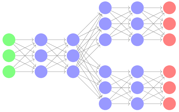
Figure 1: Example of MTNN with $2$ tasks. On the left half of the figure there is $\mathrm{N}_{0}$ (with input layer in green); on the right half of the figure there are $\mathrm{N}_{1}$ and $\mathrm{N}_{2}$ (with output layers in red).

2.1 Loss Differentiation and Multiple Tasks

In MTL, the loss function of a model typically is a weighted sum of different losses, evaluated with respect to each task. In Section 2.1 below, we introduce the symbols and the formalization we use to describe the aggregated loss and the task-specific losses of a MTNN, as well as the batches of corresponding input-output pairs. In this work, we always assume that the task-specific loss functions of the MTNN, and hence the aggregated loss also, are differentiable functions with respect to all the NN parameters.

[Aggregated and task-specific batches and losses] Let $\mathrm{N}$ be a MTNN as in Definition 2.1 and let $\mathcal{B}\subset\mathbb{R}^{n}\times\mathbb{R}^{m}$ be a batch of input-output pairs for ${\rm N}$, where $m=\sum_{k=1}^{K}m_{k}$; a batch is always assumed finite and non-empty. Then, we introduce the following notations:

1. we denote by $\mathcal{B}^{k}\subset\mathbb{R}^{n}\times\mathbb{R}^{m_{k}}$ the batch of input-output pairs related to the $k^{\rm th}$ task of ${\rm N}$ obtained from the batch $\mathcal{B}$; i.e.:

   $$\mathcal{B}^{k}:=\left\{(\boldsymbol{x},\boldsymbol{y}_{k})\in\mathbb{R}^{n}\times\mathbb{R}^{m_{k}}\left.\right|(\boldsymbol{x},\boldsymbol{y})\in\mathcal{B}\right\},\quad k=1,\ldots,K,$$

   where $\,\boldsymbol{y}_{k}=(y_{1}^{(k)},\ldots,y_{m_{k}}^{(k)})^{T}$ and $\,\boldsymbol{y}=(\boldsymbol{y}_{1}^{T},\ldots,\boldsymbol{y}_{K}^{T})^{T}\in\mathbb{R}^{m}$;

2. we denote by $\ell_{k}:\mathrm{P}^{*}(\mathbb{R}^{n}\times\mathbb{R}^{m_{k}})\times\mathbb{R}^{p_{0}+p_{k}}\rightarrow\mathbb{R}$ a loss function defined for the task $k$ of ${\rm N}$, for each $k=1,\ldots,K$, where $\mathrm{P}^{*}(A)$ denotes the set of finite and non-empty subsets of $A$, for each set $A$. For example, assuming $\ell_{k}$ as the Mean Square Error (MSE), we have that

   $$\ell_{k}(\mathcal{B}^{k};\boldsymbol{w}_{0},\boldsymbol{w}_{k})=\frac{1}{|\mathcal{B}^{k}|}\sum_{(\boldsymbol{x},\boldsymbol{y}_{k})\in\mathcal{B}^{k}}\left(\widehat{\boldsymbol{F}}_{k}(\widehat{\boldsymbol{F}}_{0}(\boldsymbol{x};\boldsymbol{w}_{0});\boldsymbol{w}_{k})-\boldsymbol{y}_{k}\right)^{2}\,,$$

   for each batch $\mathcal{B}^{k}\subset\mathbb{R}^{n}\times\mathbb{R}^{m_{k}}$;

3. we denote by $\ell:\mathrm{P}^{*}(\mathbb{R}^{n}\times\mathbb{R}^{m})\times\mathbb{R}^{p}\rightarrow\mathbb{R}$ the aggregated loss function of $\mathrm{N}$, such that $\ell$ is a linear combination with positive coefficients of the task-specific losses $\ell_{1},\ldots,\ell_{K}$:

   (1) $$\ell(\mathcal{B};\boldsymbol{w}):=\sum_{k=1}^{K}\lambda_{k}\ell_{k}(\mathcal{B}^{k};\boldsymbol{w}_{0},\boldsymbol{w}_{k})\,,\quad{\rm with}~{}~{}\lambda_{1},\ldots,\lambda_{k}\in\mathbb{R}^{+}.$$

Our alternate training method takes inspiration both from the BCD method and from those methods based on exploiting the task-specific gradients (see Section 1). Indeed, it is easily seen that the gradient of $\ell$ with respect to the task-specific parameters of task $k$ is equal to the gradient of $\lambda_{k}\ell_{k}$, i.e.:

$$\nabla_{\boldsymbol{w}_{k}}\ell(\mathcal{B};\boldsymbol{w})=\lambda_{k}\nabla_{\boldsymbol{w}_{k}}\ell_{k}(\mathcal{B}^{k};\boldsymbol{w}_{0},\boldsymbol{w}_{k})\,,$$

for each $k=1,\ldots,K$, and for any batch $\mathcal{B}\in\mathrm{P}^{*}(\mathbb{R}^{n}\times\mathbb{R}^{m})$. Then, once observed this characteristic, it is almost immediate to notice also that the gradient of $\ell(\mathcal{B};\boldsymbol{w})$ with respect to all the task-specific parameters is just a concatenation of the $K$ gradients of the task-specific losses with respect to their own task-specific parameters (and multiplied by the coefficients), namely:

$$\nabla_{\boldsymbol{w}_{\rm ts}}\ell(\mathcal{B};\boldsymbol{w})=\begin{bmatrix}\lambda_{1}\nabla_{\boldsymbol{w}_{1}}\ell_{1}(\mathcal{B}^{1};\boldsymbol{w}_{0},\boldsymbol{w}_{1})\\ \vdots\\ \lambda_{K}\nabla_{\boldsymbol{w}_{K}}\ell_{K}(\mathcal{B}^{K};\boldsymbol{w}_{0},\boldsymbol{w}_{K})\end{bmatrix}\,,$$

for each $\mathcal{B}\in\mathrm{P}(\mathbb{R}^{n}\times\mathbb{R}^{m})$, where $\boldsymbol{w}_{\rm ts}\in\mathbb{R}^{p_{\rm ts}}$ is the vector denoting the concatenation of all the task-specific parameters; i.e.:

$$\boldsymbol{w}_{\rm ts}:=(\boldsymbol{w}_{1}^{T},\ldots,\boldsymbol{w}_{K}^{T})^{T}\in\mathbb{R}^{p_{\rm ts}}\,,\quad{\rm with}~{}~{}p_{\rm ts}=\sum_{k=1}^{K}p_{k}.$$

As a consequence of these results, we see in Proposition 2.2 that for any batch $\mathcal{B}$ the two anti-gradients of $\ell$ with respect to the shared parameters and the task-specific parameters, respectively, identify two descent directions for $\ell(\mathcal{B};\boldsymbol{w})$ at $\boldsymbol{w}$ that update only the corresponding subset of NN weights; moreover, the direction based on the task-specific gradient is a descent direction for all the task-specific losses too. The proof of the proposition is omitted, since it is trivial.

Proposition 2.2 (Gradients and Descent Directions).

Let $\mathrm{N}$ be a MTNN as in Definition 2.1 and let $\ell,\ell_{1},\ldots,\ell_{K}$ be the losses in (1). Let $\boldsymbol{w}\in\mathbb{R}^{p}$ be the vector of trainable parameters of $\mathrm{N}$; specifically, $\boldsymbol{w}$ is the concatenation of the shared parameters $\boldsymbol{w}_{0}\in\mathbb{R}^{p_{0}}$ and the task-specific parameters $\boldsymbol{w}_{\rm ts}\in\mathbb{R}^{p_{\rm ts}}$:

$$\boldsymbol{w}=\begin{bmatrix}\boldsymbol{w}_{0}\\ \boldsymbol{w}_{\rm ts}\end{bmatrix}\,.$$

Then, for each fixed batch $\mathcal{B}$ the vectors

(2) $$\begin{bmatrix}-\nabla_{\boldsymbol{w}_{0}}\ell(\mathcal{B};\boldsymbol{w})\\ \boldsymbol{0}\end{bmatrix}\,,\ \begin{bmatrix}\boldsymbol{0}\\ -\nabla_{\boldsymbol{w}_{\rm ts}}\ell(\mathcal{B};\boldsymbol{w})\end{bmatrix}\in\mathbb{R}^{p}$$

are descent directions for the loss $\ell(\mathcal{B};\boldsymbol{w})$ at $\boldsymbol{w}$, if $\nabla_{\boldsymbol{w}_{0}}\ell(\mathcal{B};\boldsymbol{w})\neq\boldsymbol{0}\in\mathbb{R}^{p_{0}}$ and $\nabla_{\boldsymbol{w}_{\rm ts}}\ell(\mathcal{B};\boldsymbol{w})\neq\boldsymbol{0}\in\mathbb{R}^{p_{\rm ts}}$, respectively. Moreover, $(\boldsymbol{0},-\nabla_{\boldsymbol{w}_{k}}\ell_{k}(\mathcal{B}^{k};\boldsymbol{w}_{0},\boldsymbol{w}_{k}))$ (subvector of the first vector in (2)) is also a descent direction for $\ell_{k}(\mathcal{B}^{k};\boldsymbol{w}_{0},\boldsymbol{w}_{k})$, for each $k=1,\ldots,K$.

We conclude this section remarking the different implications of the two descent directions (2):

• $\boldsymbol{w}_{0}$-based direction: it is a descent direction for $\ell(\mathcal{B};\boldsymbol{w})$ that update the shared parameters only. It allows to reduce the loss with respect to the weights that affects all the tasks, then there are no guarantees of reducing all the task-specific losses too;

• $\boldsymbol{w}_{\rm ts}$-based direction: is a descent direction for $\ell(\mathcal{B};\boldsymbol{w})$ but also for all the task-specific losses $\ell_{1},\ldots,\ell_{K}$, and it updates the task-specific parameters only. It allows to reduce both the main loss and the task-specific losses with respect to the weights $\boldsymbol{w}_{1},\ldots,\boldsymbol{w}_{K}$ that affect only the losses $\ell_{1},\ldots,\ell_{K}$, respectively (i.e., only the corresponding tasks).

Starting from these properties, in the next section we formulate new alternate training procedures (both deterministic and stochastic), proving for convergence properties for each one.

3 Alternate Training

Proposition 2.2 defines two alternative descent directions for the loss function. Devising a training procedure based on the alternate usage of these directions or their stochastic estimators may yield the following practical advantages.

1. Alternate training for reduced memory usage and computational costs. The advantage of the alternate training concerning memory is almost evident. Indeed, at each step, an alternate procedure requires the storage of a gradient $\nabla_{\boldsymbol{w}_{0}}$ with dimension $p_{0}$ or a gradient $\nabla_{\boldsymbol{w}_{\rm ts}}$ with dimension $p_{\rm ts}$; in both cases, the gradient has dimension smaller than the “global” gradient computed with respect to all the NN’s weights (i.e., with dimension $p=p_{0}+p_{\rm ts}$). Nonetheless, this property might be not that important if $p_{0}\approx p$ and $p_{\rm ts}\approx 0$ (or vice-versa) and/or if the hardware is powerful enough to handle the global gradient of the MTNN without difficulties.

   We further observe that the computation of $\nabla_{\boldsymbol{w}_{\rm ts}}$ is cheaper than the computation of both $\nabla_{\boldsymbol{w}_{0}}$ and $\nabla_{\boldsymbol{w}}$, since only the task-specific layers of the NN are involved; then, the cost of one epoch of training is lower with an alternate procedure than with a classic one.

2. Alternate training for better generalization abilities of MTNNs. Another advantage of a training procedure characterized by some steps performed only with respect to $\boldsymbol{w}_{\rm ts}$ (i.e., with respect to the $K$ tasks independently) may be that of improving the generalization abilities and the performance of the trained MTNN. Indeed, relying on the $\boldsymbol{w}_{\rm ts}$-based direction, this approach partially reduces the typical difficulty of MTL models about selecting a direction that is not a descent direction for all the tasks, and therefore reduces the possibility of having an increase of some losses despite the overall objective function decreases (see Section 1). This interesting regularization property is illustrated in the numerical experiments of Section 4.

The idea of an alternate training can be realized in many different ways. In this work, we define alternate training methods which are modifications of a classical Stochastic Gradient (SG) procedure. They can be extended also to other optimization procedures, but we deserve these generalizations to future work.

In the next subsections we define and analyze a couple of alternate training strategies. For the convergence analyses, we will use several times the following well known inequality (e.g., see the Descent Lemma in [3, Proposition A.24]):

(3) $$\ell(\,\cdot\,;\,\boldsymbol{w}+\eta\boldsymbol{d})\leq\ell(\,\cdot\,;\,\boldsymbol{w})~{}+~{}\eta\,\nabla\ell(\,\cdot\,;\,\boldsymbol{w})^{T}\boldsymbol{d}+\frac{L}{2}\,\eta^{2}\,\|\boldsymbol{d}\|^{2},$$

which holds for differentiable functions satisfying the Lipschitz continuity condition

$$\|\nabla\ell(\,\cdot\,;\,\boldsymbol{w})-\nabla\ell(\,\cdot\,;\,\boldsymbol{z})\|\leq\,L\|\boldsymbol{w}-\boldsymbol{z}\|.$$

Where not explicitly specified, as above, gradients are taken with respect to all the parameters $\boldsymbol{w}$.

3.1 Simple Alternate Training

The Simple Alternate Training (SAT) me-thod is a two steps iterative process that alternately updates $\boldsymbol{w}_{0}$ and $\boldsymbol{w}_{\rm ts}$ in a MTNN. The variable $\boldsymbol{w}_{0}$ is updated at each iteration using a stochastic estimator of $\nabla_{\boldsymbol{w}_{0}}\ell$, while $\boldsymbol{w}_{\rm ts}$ is updated using a stochastic estimator of $\nabla_{\boldsymbol{w}_{\rm ts}}\ell$. In what follows we denote the training set as $\mathcal{T}$. We name SAT-SG this procedure in order to emphasize the relationship with SG, and we describe one iteration in Algorithm 1.

Algorithm 1 SAT-SG - Simple Alternate Training for MTNNs with SG

Data:

$(\boldsymbol{w}_{0},\boldsymbol{w}_{\rm ts})=\boldsymbol{w}^{(i)}$ (current iterate for the trainable parameters), $\mathcal{T}$ (training set), $B$ (mini-batch size), $\eta_{i}$ (learning rate), $\ell$ (loss function defined in (1)).

Iteration $i$:

1:  Sample randomly a batch $\mathcal{B}_{1}$ from $\mathcal{T}$ s.t. $|\mathcal{B}_{1}|=B$

2:  $\boldsymbol{w}_{0}\leftarrow\boldsymbol{w}_{0}-\eta_{i}\nabla_{\boldsymbol{w}_{0}}\ell(\mathcal{B}_{1};\boldsymbol{w}^{(i)})$

3:  $\boldsymbol{z}^{(i)}\leftarrow(\boldsymbol{w}_{0},\boldsymbol{w}_{\rm ts})$

4:  Sample randomly a batch $\mathcal{B}_{2}$ from $\mathcal{T}$ s.t. $|\mathcal{B}_{2}|=B$

5:  $\boldsymbol{w}_{\rm ts}\leftarrow\boldsymbol{w}_{\rm ts}-\eta_{i}\nabla_{\boldsymbol{w}_{\rm ts}}\ell(\mathcal{B}_{2};\boldsymbol{z}^{(i)})$

6:  $\boldsymbol{w}^{(i+1)}\leftarrow(\boldsymbol{w}_{0},\boldsymbol{w}_{\rm ts})$

7:  return  $\boldsymbol{w}^{(i+1)}$  (updated iterate for MTNN’s weights)

We prove the convergence properties of SAT-SG in both cases, deterministic (Theorem 3.3) and stochastic (Theorem 3.7). We consider constant learning rates and diminishing learning rates satisfying the following conditions:

(4) $$a)~{}~{}~{}\sum_{i=0}^{\infty}\eta_{i}=\infty\,,\qquad\qquad b)~{}~{}~{}\sum_{i=0}^{\infty}\eta_{i}^{2}<\infty\,.$$

Starting with the deterministic case, we first see in Lemma 3.1 that, using any fixed batch of data $\mathcal{B}_{1}=\mathcal{B}_{2}$ of size $B$, Algorithm 1 reduces the value of the loss function $\ell(\mathcal{B};\boldsymbol{w})$ for sufficiently small learning rates $\eta_{i}$. Then, in Theorem 3.3 we exploit this result to prove the convergence of SAT-SG in the full sample case, i.e. setting $\mathcal{B}_{1}\equiv\mathcal{B}_{2}\equiv\mathcal{T}$.

Lemma 3.1.

Given $\boldsymbol{w}^{(i)}\in\mathbb{R}^{p}$, let $\boldsymbol{z}^{(i)}$ and $\boldsymbol{w}^{(i+1)}$, be the two vectors computed by Algorithm 1 with $\mathcal{B}_{1}\equiv\mathcal{B}_{2}\equiv\mathcal{B}$ and $|\mathcal{B}|=B$. Then, if $\nabla\ell(\,\cdot\,;\boldsymbol{w})$ is Lipschitz continuous with Lipschitz constant $L$, and $0<\eta_{i}<2\,(1-\mu)/L$ with $\mu\in(0,1)$, the vector $\boldsymbol{d}=(\boldsymbol{w}^{(i+1)}-\boldsymbol{w}^{(i)})/\eta_{i}$ satisfies

(5) $$-\nabla\ell(\mathcal{B};\boldsymbol{w}^{(i)})^{T}\boldsymbol{d}~{}>~{}\mu\,\|\nabla\ell(\mathcal{B};\boldsymbol{w}^{(i)})\|^{2}$$

and

(6) $$\|\boldsymbol{d}\|~{}\leq~{}(1+\eta_{i}L)\,\|\nabla\ell(\mathcal{B};\boldsymbol{w}^{(i)})\|.$$

Further, for sufficiently small values of $\eta_{i}$, e.g. $0<\eta_{i}<2\,\min\,\{\mu/9\,,1-\mu\}/L$, the following descent property holds:

(7) $$\ell(\mathcal{B};\boldsymbol{w}^{(i+1)})\,=\,\ell(\mathcal{B};\boldsymbol{w}^{(i)}+\eta_{i}\boldsymbol{d})~{}\leq~{}\ell(\mathcal{B};\boldsymbol{w}^{(i)})\,-\,\eta_{i}\,C_{i}\,\|\nabla\ell(\mathcal{B};\boldsymbol{w}^{(i)})\|^{2}$$

with

$$C_{i}=\mu-\frac{L}{2}\,\eta_{i}\,(1+\eta_{i}L)^{2}>0\,.$$

Proof 3.2.

To simplify the writing of the proof we set $\boldsymbol{z}^{(i)}:=\boldsymbol{z}$, $\boldsymbol{w}^{(i)}:=\boldsymbol{w}$, $\boldsymbol{w}^{(i+1)}:=\boldsymbol{w}_{new}$. Then,

[i.] shared parameters update:

$$\boldsymbol{z}=\begin{bmatrix}{\boldsymbol{z}_{0}}\\ \boldsymbol{z}_{\rm ts}\end{bmatrix}=\boldsymbol{w}+\eta_{i}\begin{bmatrix}-\nabla_{\boldsymbol{w}_{0}}\ell(\mathcal{B};\boldsymbol{w})\\ \boldsymbol{0}\end{bmatrix}=\begin{bmatrix}\boldsymbol{w}_{0}-\eta_{i}\nabla_{\boldsymbol{w}_{0}}\ell(\mathcal{B};\boldsymbol{w})\\ \boldsymbol{w}_{\rm ts}\end{bmatrix},$$

[ii.] task-specific parameters update:

$$\boldsymbol{w}_{\rm new}=\boldsymbol{z}+\eta_{i}\begin{bmatrix}\boldsymbol{0}\\ -\nabla_{\boldsymbol{w}_{\rm ts}}\ell(\mathcal{B};\boldsymbol{z})\end{bmatrix}=\begin{bmatrix}\boldsymbol{w}_{0}-\eta_{i}\nabla_{\boldsymbol{w}_{0}}\ell(\mathcal{B};\boldsymbol{w})\\ \boldsymbol{w}_{\rm ts}-\eta_{i}\nabla_{\boldsymbol{w}_{\rm ts}}\ell(\mathcal{B};\boldsymbol{z})\\ \end{bmatrix}=\boldsymbol{w}+\eta_{i}\begin{bmatrix}-\nabla_{\boldsymbol{w}_{0}}\ell(\mathcal{B};\boldsymbol{w})\\ -\nabla_{\boldsymbol{w}_{\rm ts}}\ell(\mathcal{B};\boldsymbol{z})\\ \end{bmatrix}.$$

Rewriting $\boldsymbol{d}$ as:

$$\boldsymbol{d}=\begin{bmatrix}-\nabla_{\boldsymbol{w}_{0}}\ell(\mathcal{B};\boldsymbol{w})\\ -\nabla_{\boldsymbol{w}_{\rm ts}}\ell(\mathcal{B};\boldsymbol{z})\\ \end{bmatrix}\pm\begin{bmatrix}\boldsymbol{0}\\ -\nabla_{\boldsymbol{w}_{\rm ts}}\ell(\mathcal{B};\boldsymbol{w})\end{bmatrix}=-\nabla\ell(\mathcal{B};\boldsymbol{w})+\begin{bmatrix}\boldsymbol{0}\\ \nabla_{\boldsymbol{w}_{\rm ts}}\ell(\mathcal{B};\boldsymbol{w})-\nabla_{\boldsymbol{w}_{\rm ts}}\ell(\mathcal{B};\boldsymbol{z})\\ \end{bmatrix},$$

it follows that

$$\begin{split}-\nabla\ell(\mathcal{B};\boldsymbol{w})^{T}\boldsymbol{d}&=\|\nabla\ell(\mathcal{B};\boldsymbol{w})\|^{2}-\nabla_{\boldsymbol{w}_{\rm ts}}\ell(\mathcal{B};\boldsymbol{w})^{T}\left(\,\nabla_{\boldsymbol{w}_{\rm ts}}\ell(\mathcal{B};\boldsymbol{w})-\nabla_{\boldsymbol{w}_{\rm ts}}\ell(\mathcal{B};\boldsymbol{z})\,\right)\\ &\geq\|\nabla\ell(\mathcal{B};\boldsymbol{w})\|^{2}-L\,\|\nabla_{\boldsymbol{w}_{\rm ts}}\ell(\mathcal{B};\boldsymbol{w})\|\,\|\boldsymbol{w}-\boldsymbol{z}\|\\ &=\|\nabla\ell(\mathcal{B};\boldsymbol{w})\|^{2}-\eta_{i}L\,\|\nabla_{\boldsymbol{w}_{\rm ts}}\ell(\mathcal{B};\boldsymbol{w})\|\,\|\nabla_{\boldsymbol{w}_{0}}\ell(\mathcal{B};\boldsymbol{w})\|\\ &=\|\nabla_{\boldsymbol{w}_{0}}\ell(\mathcal{B};\boldsymbol{w})\|^{2}+\|\nabla_{\boldsymbol{w}_{\rm ts}}\ell(\mathcal{B};\boldsymbol{w})\|^{2}-\eta_{i}L\,\|\nabla_{\boldsymbol{w}_{\rm ts}}\ell(\mathcal{B};\boldsymbol{w})\|\,\|\nabla_{\boldsymbol{w}_{0}}\ell(\mathcal{B};\boldsymbol{w})\|\\ &>\|\nabla_{\boldsymbol{w}_{0}}\ell(\mathcal{B};\boldsymbol{w})\|^{2}+\|\nabla_{\boldsymbol{w}_{\rm ts}}\ell(\mathcal{B};\boldsymbol{w})\|^{2}-2(1-\mu)\,\|\nabla_{\boldsymbol{w}_{\rm ts}}\ell(\mathcal{B};\boldsymbol{w})\|\,\|\nabla_{\boldsymbol{w}_{0}}\ell(\mathcal{B};\boldsymbol{w})\|\\ &=\mu\,(\,\|\nabla_{\boldsymbol{w}_{0}}\ell(\mathcal{B};\boldsymbol{w})\|^{2}\,+\|\nabla_{\boldsymbol{w}_{\rm ts}}\ell(\mathcal{B};\boldsymbol{w})\|^{2}\,)+\\ &\quad\;(1-\mu)\,(\,\|\nabla_{\boldsymbol{w}_{\rm ts}}\ell(\mathcal{B};\boldsymbol{w})\|\,-\,\|\nabla_{\boldsymbol{w}_{0}}\ell(\mathcal{B};\boldsymbol{w})\|\,)^{2}\\ &\geq\mu\left(\,\|\nabla_{\boldsymbol{w}_{0}}\ell(\mathcal{B};\boldsymbol{w})\|^{2}+\|\nabla_{\boldsymbol{w}_{\rm ts}}\ell(\mathcal{B};\boldsymbol{w})\|^{2}\,\right)\,,\end{split}$$

where in the last inequalities we used the assumptions $\mu\in(0,1)$ and $0<\eta_{i}L<2(1-\mu).$ This complete the proof of (5).

To obtain (6) we proceed as follows:

$$\begin{split}\|\boldsymbol{d}\|^{2}&=\|\nabla\ell(\mathcal{B};\boldsymbol{w})\|^{2}+\|\,\nabla_{\boldsymbol{w}_{\rm ts}}\ell(\mathcal{B};\boldsymbol{w})-\nabla_{\boldsymbol{w}_{\rm ts}}\ell(\mathcal{B};\boldsymbol{z})\,\|^{2}\,+\\ &~{}~{}~{}~{}\,2\,\nabla_{\boldsymbol{w}_{\rm ts}}\ell(\mathcal{B};\boldsymbol{w})^{T}\left(\,\nabla_{\boldsymbol{w}_{\rm ts}}\ell(\mathcal{B};\boldsymbol{z})-\nabla_{\boldsymbol{w}_{\rm ts}}\ell(\mathcal{B};\boldsymbol{w})\,\right)\\ &\leq\|\nabla\ell(\mathcal{B};\boldsymbol{w})\|^{2}+L^{2}\|\boldsymbol{w}-\boldsymbol{z}\|^{2}+2L\,\|\nabla\ell(\mathcal{B};\boldsymbol{w})\|\,\|\boldsymbol{w}-\boldsymbol{z}\|\\ &=\left(\,\|\nabla\ell(\mathcal{B};\boldsymbol{w})\|\,+L\,\|\boldsymbol{w}-\boldsymbol{z}\|\,\right)^{2}\,=\,\left(\,\|\nabla\ell(\mathcal{B};\boldsymbol{w})\|\,+\eta_{i}L\,\|\nabla_{\boldsymbol{w}_{0}}\ell(\mathcal{B};\boldsymbol{w})\|\,\right)^{2}\\ &\leq\,(1+\eta_{i}L)^{2}\,\|\nabla\ell(\mathcal{B};\boldsymbol{w})\|^{2}.\end{split}$$

Finally, the descent property (7) is easily obtained by recalling inequality (3) and using (5) and (6) in it:

$$\begin{split}\ell(\mathcal{B};\boldsymbol{w}+\eta_{i}\boldsymbol{d})-\ell(\mathcal{B};\boldsymbol{w})&~{}\leq~{}\eta_{i}\,\nabla\ell(\mathcal{B};\boldsymbol{w})^{T}\boldsymbol{d}+\frac{L}{2}\,\eta_{i}^{2}\,\|\boldsymbol{d}\|^{2}\\ &~{}\leq~{}-\eta_{i}\,\mu\,\|\nabla\ell(\mathcal{B};\boldsymbol{w})\|^{2}+\frac{L}{2}\,\eta_{i}^{2}\,(1+\eta_{i}L)^{2}\,\|\nabla\ell(\mathcal{B};\boldsymbol{w})\|^{2}\\ &~{}=~{}-\eta_{i}\,\left(\mu-\frac{L}{2}\,\eta_{i}\,(1+\eta_{i}L)^{2}\right)\,\|\nabla\ell(\mathcal{B};\boldsymbol{w})\|^{2}.\end{split}$$

To conclude the proof we observe that the constants $C_{i}=\mu-\frac{L}{2}\,\eta_{i}\,(1+\eta_{i}L)^{2}$ are positive for sufficiently small values of $\eta_{i}$. For example, recalling that by assumption $\mu\in(0,1)$ and $0<\eta_{i}\,L<2(1-\mu)<2$, we also have $(1+\eta_{i}L)^{2}<9$. Then the claim is surely true if $0<\eta_{i}<2\,\min\,\{\mu/9\,,1-\mu\}/L$.

From now on, to shorten the notation, we will omit to explicitly indicate the dependence of the loss function from the batch of data when this coincides with the whole training set (i.e., $\mathcal{B}\equiv\mathcal{T}$), namely we will write $\ell(\boldsymbol{w})$ for $\ell(\mathcal{T};\boldsymbol{w})$, and $\nabla\ell(\boldsymbol{w})$ for $\nabla\ell(\mathcal{T};\boldsymbol{w})$.

Theorem 3.3 (SAT-SG Convergence - Deterministic).

Given $\boldsymbol{w}^{(0)}\in\mathbb{R}^{p}$ and a bounded below loss function $\ell$, with lower bound $\ell_{low}$, let $\{\boldsymbol{w}^{(i)}\}_{i\geq 0}\subset\mathbb{R}^{p}$ be the sequence generated by the SAT-SG method with $B=|\mathcal{T}|$, i.e. $\mathcal{B}_{1}\equiv\mathcal{B}_{2}\equiv\mathcal{T}$ for all $i$ and

$$\boldsymbol{w}^{(i+1)}=\boldsymbol{w}^{(i)}-\eta_{i}\begin{bmatrix}\nabla_{\boldsymbol{w}_{0}}\ell(\boldsymbol{w}^{(i)})\\ \nabla_{\boldsymbol{w}_{\rm ts}}\ell(\boldsymbol{z}^{(i)})\\ \end{bmatrix},~{}~{}i\geq 0,$$

with

$$\boldsymbol{z}^{(i)}=\boldsymbol{w}^{(i)}-\eta_{i}\begin{bmatrix}\nabla_{\boldsymbol{w}_{0}}\ell(\boldsymbol{w}^{(i)})\\ \boldsymbol{0}\end{bmatrix}.$$

Then, under the assumptions of Lemma 3.1, and for learning rates satisfying condition (4.a), any limit point of $\{\boldsymbol{w}^{(i)}\}_{i\geq 0}$ is stationary for $\ell$.

Proof 3.4.

The thesis holds trivially if $\nabla\ell(\boldsymbol{w}^{(\bar{i})})=\boldsymbol{0}$ for some finite index $\bar{i}$, yielding $\boldsymbol{w}^{(i)}=\boldsymbol{w}^{(\bar{i})}$ for all $i\geq\bar{i}$. So we consider the more general case in which $\nabla\ell(\boldsymbol{w}^{(i)})\neq\boldsymbol{0}$ for all $i\geq 0$. Now, let us observe that Lemma 3.1 holds with $\mathcal{B}=\mathcal{T}$, and therefore

(8) $$\ell(\boldsymbol{w}^{(i+1)})\,-\,\ell(\boldsymbol{w}^{(i)})~{}\leq~{}-\eta_{i}\,C_{i}\,\|\nabla\ell(\boldsymbol{w}^{(i)})\|^{2}~{}<~{}0,~{}~{}i=0,1,2,\ldots$$

Then, using (8) and the boundedness from below of $\ell$, the sequence $\{\ell(\boldsymbol{w}^{(i)})\}_{i\geq 0}$ results to be decreasing and convergent. Further, summing up for $i=0$ to infinity both sides of the first inequality in (8), we easily attain

$$\sum_{i=0}^{\infty}C_{i}\eta_{i}\|\nabla\ell(\boldsymbol{w}^{(i)})\|^{2}\leq\ell(w^{(0)})-\ell_{low}\,,\quad{\rm with}\quad C_{i}=\mu-\frac{L}{2}\,\eta_{i}\,(1+\eta_{i}L)^{2}>0\,.$$

Under the assumptions of Lemma 3.1 $C_{i}$ is bounded away from zero, then the previous inequality and the first condition in (4) ensure that $\|\nabla\ell(\boldsymbol{w}^{(i)})\|\rightarrow 0$. Finally, by continuity, at any limit point $\bar{\boldsymbol{w}}$ of $\{\boldsymbol{w}^{(i)}\}_{i\geq 0}$ it must be $\nabla\ell(\bar{\boldsymbol{w}})=\boldsymbol{0}$.

We remark that since $\sum_{i=0}^{\infty}\eta=\infty$, the case of fixed learning rates is included in Theorem 3.3.

Now, we study the convergence properties of SAT-SG in the fully stochastic case; i.e., with $B<|\mathcal{T}|$ and $\mathcal{B}_{1}\neq\mathcal{B}_{2}$.

Lemma 3.5 (SAT-SG - Stochastic).

Let $\{\boldsymbol{w}^{(i)}\}_{i\geq 0},\{\boldsymbol{z}^{(i)}\}_{i\geq 0}\subset\mathbb{R}^{p}$ be two sequences generated by the SAT-SG method, and $\{\eta_{i}\}_{i\geq 0}$ be the sequence of used learning rates. Let $\mathcal{A}_{i}$ denote the $\sigma$-algebra induced by $\boldsymbol{w}^{(0)},\boldsymbol{z}^{(0)}$, $\boldsymbol{w}^{(1)},\boldsymbol{z}^{(1)}$, …, $\boldsymbol{w}^{(i)}$, and $\mathcal{A}_{i+\frac{1}{2}}$ the $\sigma$-algebra induced by $\boldsymbol{w}^{(0)},\boldsymbol{z}^{(0)}$, $\boldsymbol{w}^{(1)},\boldsymbol{z}^{(1)}$, …, $\boldsymbol{w}^{(i)},\boldsymbol{z}^{(i)}$.

Assume that the batches $\mathcal{B}_{1}$ and $\mathcal{B}_{2}$ are sampled randomly and uniformly, that there exist two positive constants $M_{1}$ and $M_{2}$ such that

(9) $$\mathbb{E}[\|\nabla_{\boldsymbol{w}_{0}}\ell(\mathcal{B};\boldsymbol{w}^{(i)})\|^{2}|\mathcal{A}_{i}]\leq M_{2}\,\|\nabla_{\boldsymbol{w}_{0}}\ell(\boldsymbol{w}^{(i)})\|^{2}+M_{1}$$

(10) $$\mathbb{E}[\|\nabla_{\boldsymbol{w}_{\rm ts}}\ell(\mathcal{B};\boldsymbol{z}^{(i)})\|^{2}|\mathcal{A}_{i+\frac{1}{2}}]\leq M_{2}\,\|\nabla_{\boldsymbol{w}_{\rm ts}}\ell(\boldsymbol{z}^{(i)})\|^{2}+M_{1}$$

for any batch of data $\mathcal{B}$, and that $\nabla\ell(\,\cdot\,;\boldsymbol{w})$ is Lipschitz continuous with Lipschitz constant $L$.

Then for sufficiently small values of $\eta_{i}$, e.g. $0<\eta_{i}<\,\frac{1}{L}\min\,\{1,\,\frac{2}{M_{2}}\,\}$ for any $i\geq 0$, the following property holds:

(11) $$\mathbb{E}[\ell(\boldsymbol{w}^{(i+1)})|\mathcal{A}_{i}]\,\leq\,\ell(\boldsymbol{w}^{(i)})-\,\eta_{i}\,(1-L\,\eta_{i})\,G_{i}\,\|\nabla\ell(\boldsymbol{w}^{(i)})\|^{2}+\eta_{i}^{2}LM_{1}$$

with $~{}G_{i}=1-\frac{L}{2}\,\eta_{i}\,M_{2}>0\,.$

Proof 3.6.

First, we consider the updating of the shared parameters $\boldsymbol{w}_{0}$ (see steps 2 and 3 of Algorithm 1), and use inequality (3) to obtain

$$\ell(\boldsymbol{z}^{(i)})\leq\ell(\boldsymbol{w}^{(i)})~{}+~{}\eta_{i}\,\nabla\ell(\boldsymbol{w^{(i)}})^{T}\begin{bmatrix}-\nabla_{\boldsymbol{w}_{0}}\ell(\mathcal{B}_{1};\boldsymbol{w}^{(i)})\\ \boldsymbol{0}\end{bmatrix}+\frac{L}{2}\,\eta_{i}^{2}\,\|\nabla_{\boldsymbol{w}_{0}}\ell(\mathcal{B}_{1};\boldsymbol{w}^{(i)})\|^{2}.\\$$

Then, taking the conditioned expected value on both sides, exploiting assumption (9) and the fact that the subsampled gradient $\nabla_{\boldsymbol{w}_{0}}\ell(\mathcal{B}_{1};\boldsymbol{w}^{(i)})$ is an unbiased estimator, we have:

$$\begin{split}\mathbb{E}[\ell(\boldsymbol{z}^{(i)})|\mathcal{A}_{i}]&~{}\leq~{}\ell(\boldsymbol{w}^{(i)})-\eta_{i}\,\nabla_{\boldsymbol{w}_{0}}\ell(\boldsymbol{w^{(i)}})^{T}\mathbb{E}[\nabla_{\boldsymbol{w}_{0}}\ell(\mathcal{B}_{1};\boldsymbol{w}^{(i)})|\mathcal{A}_{i}]~{}+\\ &\quad~{}~{}~{}\frac{L}{2}\,\eta_{i}^{2}\,\mathbb{E}[\|\nabla_{\boldsymbol{w}_{0}}\ell(\mathcal{B}_{1};\boldsymbol{w}^{(i)})\|^{2}\,|\mathcal{A}_{i}]\\ &~{}\leq~{}\ell(\boldsymbol{w}^{(i)})-\eta_{i}\,\|\nabla_{\boldsymbol{w}_{0}}\ell(\boldsymbol{w^{(i)}})\|^{2}+\frac{L}{2}\,\eta_{i}^{2}\,(M_{2}\,\|\nabla_{\boldsymbol{w}_{0}}\ell(\boldsymbol{w}^{(i)})\|^{2}+M_{1}),\end{split}$$

which, by setting $G_{i}=1-\frac{L}{2}\,\eta_{i}\,M_{2}$, can be re-written as

(12) $$\mathbb{E}[\ell(\boldsymbol{z}^{(i)})|\mathcal{A}_{i}]~{}\leq~{}\ell(\boldsymbol{w}^{(i)})-\eta_{i}\,G_{i}\,\|\nabla_{\boldsymbol{w}_{0}}\ell(\boldsymbol{w^{(i)}})\|^{2}+\frac{L}{2}\,\eta_{i}^{2}\,M_{1},$$

with $G_{i}>0$ for sufficiently small values of $\eta_{i}$.

Similarly, after updating the task-specific parameters $\boldsymbol{w}_{\rm ts}$ we have that

$$\ell(\boldsymbol{w}^{(i+1)})\leq\ell(\boldsymbol{z}^{(i)})~{}+~{}\eta_{i}\,\nabla\ell(\boldsymbol{z^{(i)}})^{T}\begin{bmatrix}\boldsymbol{0}\\ -\nabla_{\boldsymbol{w}_{\rm ts}}\ell(\mathcal{B}_{2};\boldsymbol{z}^{(i)})\end{bmatrix}+\frac{L}{2}\,\eta_{i}^{2}\,\|\nabla_{\boldsymbol{w}_{\rm ts}}\ell(\mathcal{B}_{2};\boldsymbol{z}^{(i)})\|^{2}.\\$$

Further, proceeding as before in conditioned expected values and using assumption (10), we get

(13) $$\mathbb{E}[\ell(\boldsymbol{w}^{(i+1)})|\mathcal{A}_{i+\frac{1}{2}}]~{}\leq~{}\ell(\boldsymbol{z}^{(i)})-\eta_{i}\,G_{i}\,\|\nabla_{\boldsymbol{w}_{\rm ts}}\ell(\boldsymbol{z^{(i)}})\|^{2}+\frac{L}{2}\,\eta_{i}^{2}\,M_{1}.$$

Now we observe that

$$\begin{split}\|\nabla_{\boldsymbol{w}_{\rm ts}}\ell(\boldsymbol{z^{(i)}})\|^{2}&=\|\nabla_{\boldsymbol{w}_{\rm ts}}\ell(\boldsymbol{w}^{(i)})+\nabla_{\boldsymbol{w}_{\rm ts}}\ell(\boldsymbol{z}^{(i)})-\nabla_{\boldsymbol{w}_{\rm ts}}\ell(\boldsymbol{w}^{(i)})\,\|^{2}~{}\\ &=\|\nabla_{\boldsymbol{w}_{\rm ts}}\ell(\boldsymbol{w^{(i)}})\|^{2}\,+\|\,\nabla_{\boldsymbol{w}_{\rm ts}}\ell(\boldsymbol{z}^{(i)})-\nabla_{\boldsymbol{w}_{\rm ts}}\ell(\boldsymbol{w^{(i)}})\,\|^{2}+\\ &~{}~{}~{}\,2\,\nabla_{\boldsymbol{w}_{\rm ts}}\ell(\boldsymbol{w}^{(i)})^{T}\left(\,\nabla_{\boldsymbol{w}_{\rm ts}}\ell(\boldsymbol{z}^{(i)})-\nabla_{\boldsymbol{w}_{\rm ts}}\ell(\boldsymbol{w}^{(i)})\,\right)\,\\ &\geq\,\|\nabla_{\boldsymbol{w}_{\rm ts}}\ell(\boldsymbol{w^{(i)}})\|^{2}\,-2\,\|\nabla_{\boldsymbol{w}_{\rm ts}}\ell(\boldsymbol{w}^{(i)})\|\,\|\,\nabla_{\boldsymbol{w}_{\rm ts}}\ell(\boldsymbol{w}^{(i)})-\nabla_{\boldsymbol{w}_{\rm ts}}\ell(\boldsymbol{z^{(i)}})\,\|\,\\ &\geq\,\|\nabla_{\boldsymbol{w}_{\rm ts}}\ell(\boldsymbol{w}^{(i)})\|^{2}-2L\,\eta_{i}\,\|\nabla_{\boldsymbol{w}_{\rm ts}}\ell(\boldsymbol{w}^{(i)})\|\,\|\nabla_{\boldsymbol{w}_{0}}\ell(\boldsymbol{w}^{(i)})\|;\end{split}$$

then using this last inequality in (13) we have

(14) $$\begin{split}\mathbb{E}[\ell(\boldsymbol{w}^{(i+1)})|\mathcal{A}_{i+\frac{1}{2}}]~{}\leq~{}&\ell(\boldsymbol{z}^{(i)})-\eta_{i}\,G_{i}\,\|\nabla_{\boldsymbol{w}_{\rm ts}}\ell(\boldsymbol{w^{(i)}})\|^{2}+\\ &2L\,\eta_{i}^{2}G_{i}\,\|\nabla_{\boldsymbol{w}_{\rm ts}}\ell(\boldsymbol{w}^{(i)})\|\,\|\nabla_{\boldsymbol{w}_{0}}\ell(\boldsymbol{w}^{(i)})\|+\frac{L}{2}\,\eta_{i}^{2}\,M_{1}.\end{split}$$

Finally, recalling that

$$\mathbb{E}[\ell(\boldsymbol{w}^{(i+1)})|\mathcal{A}_{i}]=\mathbb{E}[\,\mathbb{E}[\ell(\boldsymbol{w}^{(i+1)})|\mathcal{A}_{i+\frac{1}{2}}]\,|\,\mathcal{A}_{i}],$$

and combining (12) and (14) we have

$$\begin{split}\mathbb{E}[\ell(\boldsymbol{w}^{(i+1)})|\mathcal{A}_{i}]&~{}\leq~{}\mathbb{E}[\ell(\boldsymbol{z}^{(i)})|\mathcal{A}_{i}]-\eta_{i}\,G_{i}\,\|\nabla_{\boldsymbol{w}_{\rm ts}}\ell(\boldsymbol{w^{(i)}})\|^{2}+\\ &\quad\quad 2L\,\eta_{i}^{2}G_{i}\,\|\nabla_{\boldsymbol{w}_{\rm ts}}\ell(\boldsymbol{w}^{(i)})\|\,\|\nabla_{\boldsymbol{w}_{0}}\ell(\boldsymbol{w}^{(i)})\|+\frac{L}{2}\,\eta_{i}^{2}\,M_{1}\\ &~{}\leq~{}\ell(\boldsymbol{w}^{(i)})-\eta_{i}\,G_{i}\,\|\nabla_{\boldsymbol{w}_{0}}\ell(\boldsymbol{w^{(i)}})\|^{2}+\frac{L}{2}\,\eta_{i}^{2}\,M_{1}-\eta_{i}\,G_{i}\,\|\nabla_{\boldsymbol{w}_{\rm ts}}\ell(\boldsymbol{w^{(i)}})\|^{2}~{}+\\ &\quad\quad 2L\,\eta_{i}^{2}G_{i}\,\|\nabla_{\boldsymbol{w}_{\rm ts}}\ell(\boldsymbol{w}^{(i)})\|\,\|\nabla_{\boldsymbol{w}_{0}}\ell(\boldsymbol{w}^{(i)})\|+\frac{L}{2}\,\eta_{i}^{2}\,M_{1}\\ &~{}=~{}\ell(\boldsymbol{w}^{(i)})-\eta_{i}\,G_{i}\,\|\nabla\ell(\boldsymbol{w^{(i)}})\|^{2}+L\,\eta_{i}^{2}\,M_{1}~{}+\\ &\quad\quad 2L\,\eta_{i}^{2}G_{i}\,\|\nabla_{\boldsymbol{w}_{\rm ts}}\ell(\boldsymbol{w}^{(i)})\|\,\|\nabla_{\boldsymbol{w}_{0}}\ell(\boldsymbol{w}^{(i)})\|\\ &~{}\leq~{}\ell(\boldsymbol{w}^{(i)})-\eta_{i}\,G_{i}(1-L\eta_{i})\,\|\nabla\ell(\boldsymbol{w^{(i)}})\|^{2}+L\,\eta_{i}^{2}\,M_{1},\end{split}$$

where the last inequality follows easily from the relation $2ab\,\leq\,a^{2}+b^{2}.$

Inequality (11) in Lemma 3.5 paths the way for the following standard result on the convergence of stochastic gradient methods (see also Theorems 4.8 and 4.10 in [4]).

Theorem 3.7 (SAT-SG convergence - Stochastic).

Assume that the hypotheses in Lemma 3.5 hold and that the loss function $\ell$ is bounded below. Let $\ell_{low}$ be the lower bound, and $\{\boldsymbol{w}^{(i)}\}_{i\geq 0}$ be the sequence of iterates generated by Algorithm 1. Then,

i) for fixed learning rates $\eta_{i}=\eta$ such that $0<\eta<\,\frac{1}{L}\min\,\{1,\,\frac{2}{M_{2}}\,\}$, the average-squared gradients of $\ell$ satisfy the following inequality at any iteration $J\in\mathbb{N}$:

(15) $$\qquad\mathbb{E}[\frac{1}{J+1}\sum_{i=0}^{J}\|\nabla\ell(\boldsymbol{w}^{(i)})\|^{2}] \leq \frac{\eta LM_{1}}{(1-L\eta)G}+\frac{\ell(\boldsymbol{w}^{(0)})-\ell_{low}}{(J+1)\eta(1-L\eta)G}$$

(16) $$\xrightarrow{J\rightarrow\infty} \frac{\eta LM_{1}}{(1-L\eta)G},$$

with $G=1-\frac{L}{2}\,\eta\,M_{2}>0\,;$

ii) for diminishing learning rates satisfying (4), the weighted average-squared gradients of $\ell$ satisfies:

(17) $$\lim_{J\rightarrow\infty}\mathbb{E}\Big{[}\frac{1}{\sum_{i=0}^{J}\eta_{i}}\sum_{i=0}^{J}\eta_{i}\|\nabla\ell(\boldsymbol{w}^{(i)})\|^{2}\Big{]}=0.$$

Proof 3.8.

Taking the total expectation of (11) we get

$$\mathbb{E}[\ell(\boldsymbol{w}^{(i+1)})]-\mathbb{E}[\ell(\boldsymbol{w}^{(i)})]\leq-\,\eta_{i}\,(1-L\,\eta_{i})\,G_{i}\,\mathbb{E}[\|\nabla\ell(\boldsymbol{w}^{(i)})\|^{2}]+\eta_{i}^{2}LM_{1},$$

where $G_{i}=1-\frac{L}{2}\,\eta_{i}\,M_{2}$. Then summing up for $i=0$ to $i=J$ and recalling that $\ell$ is bounded from below by $\ell_{low}$ we obtain

$$\begin{split}\ell_{low}-\ell(\boldsymbol{w}^{(0)})&~{}\leq~{}\mathbb{E}[\ell(\boldsymbol{w}^{(J+1)})|]-\ell(\boldsymbol{w}^{(0)})\\ &~{}\leq~{}-\sum_{i=0}^{J}\eta_{i}\,(1-L\,\eta_{i})\,G_{i}E[\|\nabla\ell(\boldsymbol{w}^{(i)})\|^{2}]+LM_{1}\sum_{i=0}^{J}\eta_{i}^{2}.\end{split}$$

Now in case i), since $\eta_{i}=\eta$ and $G_{i}=G=1-\frac{L}{2}\,\eta\,M_{2}$ for all $i$, by rearranging the previous inequality we have

$$\mathbb{E}[\sum_{i=0}^{J}\|\nabla\ell(\boldsymbol{w}^{(i)})\|^{2}]\,\leq\,(J+1)\frac{\eta LM_{1}}{(1-L\eta)G}+\frac{\ell(\boldsymbol{w}^{(0)})-\ell_{low}}{\eta(1-L\eta)G},$$

from which (15) follows by dividing for $J+1$.

In case ii), assuming that $0<\eta_{i}<\,\frac{1}{L}\min\,\{\frac{1}{2},\,\frac{1}{M_{2}}\,\}$, we get $(1-L\eta_{i})G_{i}>\frac{1}{4}$ and

$$\sum_{i=0}^{J}\eta_{i}E[\|\nabla\ell(\boldsymbol{w}^{(i)})\|^{2}]\leq 4(\ell(\boldsymbol{w}^{(0)})-\ell_{low})+4LM_{1}\sum_{i=0}^{J}\eta_{i}^{2}.$$

Then, the second condition in (4) implies that the right hand side of the above inequality is bounded when $J$ goes to $\infty$, and (17) follows by using condition (4.a).

Comparing (15) with the corresponding result for the SG method [4, Th. 4.8], we have in the right hand side the additional factor $1/G>1$. Then, we expect a slower decrease of the average gradients than that obtained by SG. Instead, regarding the optimality gap (16) the matter is questionable, as the constant $M_{1}$ in (9)-(10) is expected to be smaller than the corresponding constant used to bound the expected value of $\|\nabla\ell(\boldsymbol{w})\|^{2}$ with SG.

3.2 Alternate training through the epochs

From the practical point of view, it can be more effective to alternate the training procedure through the epochs, since within each epoch it is assumed that the model sees all the available training samples; moreover, concerning compatibility with Deep Learning frameworks, it is easier to develop a training procedure that alternatively switches the trainable weights ($\boldsymbol{w}_{0}$ and $\boldsymbol{w}_{\rm ts}$) at given epochs instead at each mini-batch.

With an alternate training through the epochs, the weights of the NN are alternatively updated for some epochs with respect to $\boldsymbol{w}_{0}$, and for some other epochs with respect to $\boldsymbol{w}_{\rm ts}$. We can outline the procedure as follows:

• train the MTNN with SG for $E_{0}\in\mathbb{N}$ epochs, with respect to the shared parameters $\boldsymbol{w}_{0}$;

• train the MTNN with SG for $E_{\rm ts}\in\mathbb{N}$ epochs, with respect to the task-specific parameters $\boldsymbol{w}_{\rm ts}$;

• repeat until convergence (or a stopping criterion is satisfied).

So a complete cycle of alternate training (see Algorithm 2) consists of $E_{0}+E_{\rm ts}$ epochs and $t\cdot(E_{0}+E_{\rm ts})$ updating iterations, where $t\in\mathbb{N}$ is the number of used batches per epoch, tipically the integer part of $|\mathcal{T}|/B$ for a given batch size $B$. We name Alternate Through the Epochs with SG (ATE-SG) this procedure. In the rest of this section, we denote by $e$ the cycle counter and by $i$ the step (or iteration) counter, namely each cycle $e$ starts at the iterate $\boldsymbol{w}^{(i_{\rm ts})}$ with $i_{\rm ts}=(E_{0}+E_{\rm ts})\,e\,t$.

Algorithm 2 ATE-SG - Alternate Training through Epochs for MTNNs with SG

Data:

$(\boldsymbol{w}_{0}^{(i_{\rm ts})},\boldsymbol{w}_{\rm ts}^{(i_{\rm ts})})=\boldsymbol{w}^{(i_{\rm ts})}$ (current iterate for the trainable parameters), $\mathcal{T}$ (training set), $B$ (mini-batch size), $t$ (number of mini-batches per epoch), $E_{0},E_{\rm ts}$ (number of epochs for alternate training), $\{\eta_{i},~{}i=i_{\rm ts},\ldots,\,i_{\rm ts}+(E_{0}+E_{\rm ts})t-1\}$ (learning rates), $\ell$ (loss function as in Section 2.1).

Cycle $e$:

1:  $i\leftarrow i_{\rm ts}$   ( iteration counter, here $i=(E_{0}+E_{\rm ts})\,e\,t\,$)

2:  for $e_{0}=1,2,\ldots,E_{0}$ (epochs counter, shared phase) do

3:     for $\tau=1,2,\ldots,t$ do

4:        Sample randomly and uniformly a batch $\mathcal{B}_{\tau}$ from $\mathcal{T}$ s.t. $|\mathcal{B}_{\tau}|=B$

5:        $\boldsymbol{w}_{0}^{(i+1)}\leftarrow\boldsymbol{w}_{0}^{(i)}-\eta_{i}\nabla_{\boldsymbol{w}_{0}}\ell(\mathcal{B}_{\tau};\boldsymbol{w}^{(i)})$    

6:        $i\leftarrow i+1$

7:        $\boldsymbol{w}^{(i)}\leftarrow(\boldsymbol{w}_{0}^{(i)},\boldsymbol{w}_{\rm ts}^{(i_{\rm ts})})~{}~{}$

8:     end for

9:  end for

10:  $i_{0}\leftarrow i$  (here $i=i_{\rm ts}+tE_{0}$)

11:  for $e_{\rm ts}=1,2,\ldots,E_{\rm ts}$ (epochs counter, task-specific phase) do

12:     for $\tau=1,2,\ldots,t$ do

13:        Sample randomly and uniformly a batch $\mathcal{B}_{\tau}$ from $\mathcal{T}$ s.t. $|\mathcal{B}_{\tau}|=B$

14:        $\boldsymbol{w}_{\rm ts}^{(i+1)}\leftarrow\boldsymbol{w}_{\rm ts}^{(i)}-\eta_{i}\nabla_{\boldsymbol{w}_{\rm ts}}\ell(\mathcal{B}_{\tau};\boldsymbol{w}^{(i)})$

15:        $i\leftarrow i+1$

16:        $\boldsymbol{w}^{(i)}\leftarrow(\boldsymbol{w}_{0}^{(i_{0})},\boldsymbol{w}_{\rm ts}^{(i)})$

17:     end for

18:  end for

19:  $i_{\rm ts}\leftarrow i$  (here $i=i_{0}+tE_{\rm ts}$)

20:  return  $\boldsymbol{w}^{(i_{\rm ts})}$  (updated iterate after $E_{0}+E_{\rm ts}$ epochs)

To analyze the convergence properties of ATE-SG it is convenient to split the set of iteration indexes into two subsets, $I_{0}$ and $I_{\rm ts}$, corresponding to the shared phase and to the task-specific phase, respectively. In other words, gradients with respect to the shared (task-specific) parameters are evaluated at iterate $\boldsymbol{w}^{(i)}$ when $i\in I_{0}\,(I_{\rm ts})$. We will also make use of the following theorem [23].

Theorem 3.9 (Robbins-Sigmund 1971 [23]).

Let $U_{i},\beta_{i},\xi_{i},\rho_{i}$ be nonnegative $\mathcal{A}_{i}$-measurable random variables such that

$$\mathbb{E}[U_{i+1}|\mathcal{A}_{i}]\leq(1+\beta_{i})U_{i}+\xi_{i}-\rho_{i}\quad\quad i=0,1,2\ldots.$$

Then, on the set $\{\sum_{i}\beta_{i}<\infty,\sum_{i}\xi_{i}<\infty\}$, $U_{i}$ converges almost surely to a random variable $U$ and $\sum_{i}\rho_{i}<\infty$ almost surely.

We now prove the almost sure convergence of ATE-SG assuming to use diminishing learning rates.

Lemma 3.10 (ATE-SG - Stochastic).

Given $\boldsymbol{w}^{(0)}\in\mathbb{R}^{p}$, let $\{\boldsymbol{w}^{(i)}\}_{i\geq 0}\subset\mathbb{R}^{p}$ be the sequence generated by iterating ATE-SG Algorithm 2, with a diminishing sequence of learning rates $\{\eta_{i}\}_{i\geq 0}$ such that (4) holds. Assume that the loss function $\ell$ is bounded below by $\ell_{low}$, and there exist two positive constants $M_{1}$ and $M_{2}$ such that for any batch of data $\mathcal{B}$

$$\mathbb{E}[\|\nabla_{\boldsymbol{w}_{0}}\ell(\mathcal{B};\boldsymbol{w}^{(i)})\|^{2}|\mathcal{A}_{i}]\leq M_{2}\,\|\nabla_{\boldsymbol{w}_{0}}\ell(\boldsymbol{w}^{(i)})\|^{2}+M_{1},~{}~{}{\rm for}~{}i\in I_{0},$$

$$\mathbb{E}[\|\nabla_{\boldsymbol{w}_{\rm ts}}\ell(\mathcal{B};\boldsymbol{w}^{(i)})\|^{2}|\mathcal{A}_{i}]\leq M_{2}\,\|\nabla_{\boldsymbol{w}_{\rm ts}}\ell(\boldsymbol{w}^{(i)})\|^{2}+M_{1},~{}~{}{\rm for}~{}i\in I_{\rm ts},$$

where $\mathcal{A}_{i}$ denotes the $\sigma$-algebra induced by $\boldsymbol{w}^{(0)}$,…, $\boldsymbol{w}^{(i)}$, and $I_{0}$ and $I_{\rm ts}$ are the sets of iteration indexes corresponding to the shared phase and to the task-specific phase, respectively. Then

$$\lim\inf_{i\in I_{0}}||\nabla_{\boldsymbol{w}_{0}}\ell(z^{(i)})||^{2}=\lim\inf_{i\in I_{\rm ts}}||\nabla_{\boldsymbol{w}_{ts}}\ell(z^{(i)})||^{2}=0\quad\quad a.s.$$

Proof 3.11.

As in the proof of Lemma 3.5, we start by considering the updating of the shared parameters $\boldsymbol{w}_{0}$ and the inequality:

$$\ell(\boldsymbol{w}^{(i+1)})\leq\ell(\boldsymbol{w}^{(i)})~{}+~{}\eta_{i}\,\nabla\ell(\boldsymbol{w}^{(i)})^{T}\begin{bmatrix}-\nabla_{\boldsymbol{w}_{0}}\ell(\mathcal{B}_{\tau};\boldsymbol{w}^{(i)})\\ \boldsymbol{0}\end{bmatrix}+\frac{L}{2}\,\eta_{i}^{2}\,\|\nabla_{\boldsymbol{w}_{0}}\ell(\mathcal{B}_{\tau};\boldsymbol{w}^{(i)})\|^{2},\\$$

which holds for $i\in I_{0}$, and in conditioned expected values becomes

$$\begin{split}\mathbb{E}[\ell(\boldsymbol{w}^{(i+1)})|\mathcal{A}_{i}]&~{}\leq~{}\ell(\boldsymbol{w}^{(i)})-\eta_{i}\,\|\nabla_{\boldsymbol{w}_{0}}\ell(\boldsymbol{w}^{(i)})\|^{2}+\frac{L}{2}\,\eta_{i}^{2}\,(M_{2}\,\|\nabla_{\boldsymbol{w}_{0}}\ell(\boldsymbol{w}^{(i)})\|^{2}+M_{1})\\ &~{}=~{}\ell(\boldsymbol{w}^{(i)})-\eta_{i}\,G_{i}\,\|\nabla_{\boldsymbol{w}_{0}}\ell(\boldsymbol{w}^{(i)})\|^{2}+\frac{L}{2}\,\eta_{i}^{2}\,M_{1},\end{split}$$

with $G_{i}=1-\frac{L}{2}\eta_{i}M_{2}>0$ for sufficiently small values of $\eta_{i}$. Similarly, in the task-specific case, that is when $i\in I_{\rm ts}$, we have

$$\mathbb{E}[\ell(\boldsymbol{w}^{(i+1)})|\mathcal{A}_{i}]~{}\leq~{}\ell(\boldsymbol{w}^{(i)})-\eta_{i}\,G_{i}\,\|\nabla_{\boldsymbol{w}_{\rm ts}}\ell(\boldsymbol{z^{(i)}})\|^{2}+\frac{L}{2}\,\eta_{i}^{2}\,M_{1}.$$

Then, using Theorem 3.9 with $U_{i}=\ell(\boldsymbol{w}^{(i)})-\ell_{low}>0$, $\,\beta_{i}=0\,$ and $\,\xi_{i}=\frac{L}{2}\,\eta_{i}^{2}\,M_{1}$ for any $i\geq 0$, $\rho_{i}=\eta_{i}G_{i}\|\nabla_{\boldsymbol{w}_{\rm ts}}\ell(\boldsymbol{w}^{(i)})\|^{2}\,$ for  $i\in I_{\rm ts},\,$ and $\,\rho_{i}=\eta_{i}G_{i}\|\nabla_{\boldsymbol{w}_{0}}\ell(\boldsymbol{w}^{(i)})\|^{2}$  for   $i\in I_{0}$, we have that

(18) $$\sum_{i=0}^{\infty}\rho_{i}=\sum_{i\in I_{\rm ts}}\eta_{i}G_{i}\|\nabla_{\boldsymbol{w}_{\rm ts}}\ell(\boldsymbol{w}^{(i)})\|^{2}~{}+~{}\sum_{i\in I_{0}}\eta_{i}G_{i}\|\nabla_{\boldsymbol{w}_{0}}\ell(\boldsymbol{w}^{(i)})\|^{2}<\infty,$$

and the sequence $\{\ell(\boldsymbol{w}^{(i)})\}$ is convergent almost surely.

Recall now that $0<G_{0}=1-\frac{L}{2}\eta_{0}M_{2}\leq G_{i}=1-\frac{L}{2}\eta_{i}M_{2}<1$ for $\eta_{0}$ sufficiently small, hence from (18) it also holds

(19) $$\sum_{i\in I_{\rm ts}}\eta_{i}\|\nabla_{\boldsymbol{w}_{\rm ts}}\ell(\boldsymbol{w}^{(i)})\|^{2}~{}+~{}\sum_{i\in I_{0}}\eta_{i}\|\nabla_{\boldsymbol{w}_{0}}\ell(\boldsymbol{w}^{(i)})\|^{2}<\infty\quad\quad a.s.$$

Since $\sum\eta_{i}=\infty$ the thesis follows.

Theorem 3.12 (ATE-SG convergence - Stochastic).

Under the assumptions of Lemma 3.10, and using the same notations, let us further assume that there exists $M>0$ such that

(20) $$\|\nabla\ell(\mathcal{B};\boldsymbol{w}^{(i)})\|^{2}\leq M\,~{}~{}{\rm for~{}any}~{}\mathcal{B}~{}\subset\mathcal{T}.$$

Then

(21) $$\lim\inf_{i\to\infty}||\nabla\ell(\boldsymbol{w}^{(i)})||^{2}=0\quad\quad a.s.$$

Proof 3.13.

Reasoning as in Lemma 3.10, we are going to show that

$$\sum_{i=0}^{\infty}\eta_{i}\|\nabla\ell(\boldsymbol{w}^{(i)})\|^{2}<\infty\quad\quad a.s.$$

from which the thesis follows. To this aim, we first rewrite the above series as

(22) $$\begin{split}\sum_{i=0}^{\infty}\eta_{i}\|\nabla\ell(\boldsymbol{w}^{(i)})\|^{2}=&\sum_{i\in I_{\rm ts}}\eta_{i}\|\nabla_{\boldsymbol{w}_{\rm ts}}\ell(\boldsymbol{w}^{(i)})\|^{2}~{}+~{}\sum_{i\in I_{0}}\eta_{i}\|\nabla_{\boldsymbol{w}_{0}}\ell(\boldsymbol{w}^{(i)})\|^{2}+\\ &\sum_{i\in I_{\rm ts}}\eta_{i}\|\nabla_{\boldsymbol{w}_{0}}\ell(\boldsymbol{w}^{(i)})\|^{2}~{}+~{}\sum_{i\in I_{0}}\eta_{i}\|\nabla_{\boldsymbol{w}_{\rm ts}}\ell(\boldsymbol{w}^{(i)})\|^{2}.\end{split}$$

Now, recalling (19) we only need to show that the last two terms in (22) are bounded. Both terms can be treated in a very similar way, hence we will prove the result in details only for the last one. Moreover, for simplicity’s sake we consider the case $E_{0}=E_{\rm ts}=1$, where one cycle of ATE-SG consists of $t$ SG steps taken first with respect to the shared parameters $\boldsymbol{w}_{0}$, and then with respect to the task-specific parameters $\boldsymbol{w}_{\rm ts}$. This allows us to write down and exploit the following representations of the sets $I_{0}$ and $I_{\rm ts}$:

(23) $$I_{0}=[\,0:t-1\,]\,\cup\,[\,2\,t:3\,t-1\,]\,\cup\,\cdots=\displaystyle\bigcup_{e=0}^{\infty}\,[\,2\,e\,t:(2\,e+1)\,t-1\,]\quad$$

(24) $$\qquad I_{\rm ts}=[\,t:2\,t-1\,]\,\cup\,[\,3\,t:4\,t-1\,]\,\cup\,\cdots=\displaystyle\bigcup_{e=1}^{\infty}\,[\,(2\,e-1)\,t:2et-1\,].$$

Nonetheless, we remark that with a bit more technicalities the proof can be extended to the general case $E_{0}\geq 1$ and $E_{\rm ts}\geq 1$.

So, let us consider the last term in (22), which by using (23) can be rewritten as follows:

(25) $$\begin{split}\sum_{i\in I_{0}}\eta_{i}\|\nabla_{\boldsymbol{w}_{\rm ts}}\ell(\boldsymbol{w}^{(i)})\|^{2}&=\sum_{e=0}^{\infty}\sum_{\tau=0}^{t-1}\eta_{2et+\tau}\|\nabla_{\boldsymbol{w}_{\rm ts}}\ell(\boldsymbol{w}^{(2et+\tau)})\|^{2}\\ &=\sum_{\tau=0}^{t-1}\eta_{\tau}\|\nabla_{\boldsymbol{w}_{\rm ts}}\ell(\boldsymbol{w}^{(\tau)})\|^{2}+\sum_{e=1}^{\infty}\sum_{\tau=0}^{t-1}\eta_{2et+\tau}\|\nabla_{\boldsymbol{w}_{\rm ts}}\ell(\boldsymbol{w}^{(2et+\tau)})\|^{2},\end{split}$$

where, for any $e\geq 1$ and $\tau=0,1,\ldots,t-1$,

$$\begin{split}\|\nabla_{\boldsymbol{w}_{\rm ts}}\ell(\boldsymbol{w}^{(2et+\tau)})\|&\leq\|\nabla_{\boldsymbol{w}_{\rm ts}}\ell(\boldsymbol{w}^{(2et+\tau)})-\nabla_{\boldsymbol{w}_{\rm ts}}\ell(\boldsymbol{w}^{(2et-1)})\|+\|\nabla_{\boldsymbol{w}_{\rm ts}}\ell(\boldsymbol{w}^{(2et-1)})\|\\ &\leq L\|\boldsymbol{w}^{(2et+\tau)}-\boldsymbol{w}^{(2et-1)}\|+\|\nabla_{\boldsymbol{w}_{\rm ts}}\ell(\boldsymbol{w}^{(2et-1)})\|\\ &=L\,\|\eta_{2et-1}\nabla_{\boldsymbol{w}_{\rm{ts}}}\ell(\mathcal{B}_{t};\boldsymbol{w}^{(2et-1)})+\sum_{k=0}^{\tau-1}\eta_{2et+k}\nabla_{\boldsymbol{w}_{0}}\ell(\mathcal{B}_{k};\boldsymbol{w}^{(2et+k)})\,\|\\ &\quad+\|\nabla_{\boldsymbol{w}_{\rm ts}}\ell(\boldsymbol{w}^{(2et-1)})\|.\end{split}$$

The idea of the proof is that, when damped by the learning rates, gradient norms can be bounded by assumption (20). Instead, to tackle the norm of $\nabla_{\boldsymbol{w}_{\rm ts}}\ell(\boldsymbol{w}^{(2et-1)})$ we can resort to Lemma 3.10, since by (24) it is easily seen that $2et-1\in I_{\rm ts}$ for any $e\geq 1$. Then $~{}\|\nabla_{\boldsymbol{w}_{\rm ts}}\ell(\boldsymbol{w}^{(2et+\tau)})\|\leq LM\sum_{k=-1}^{\tau-1}\eta_{2et+k}+\|\nabla_{\boldsymbol{w}_{\rm ts}}\ell(\boldsymbol{w}^{(2et-1)})\|\,,$ and

(26) $$\begin{split}\|\nabla_{\boldsymbol{w}_{\rm ts}}\ell(\boldsymbol{w}^{(2et+\tau)})\|^{2}&\leq L^{2}M^{2}\,(\,\sum_{k=-1}^{\tau-1}\eta_{2et+k}\,)^{2}+\\ &\quad 2LM^{2}(\,\sum_{k=-1}^{\tau-1}\eta_{2et+k}\,)+\|\nabla_{\boldsymbol{w}_{\rm ts}}\ell(\boldsymbol{w}^{(2et-1)})\|^{2}.\end{split}$$

Now using (20) and (26) in (25) we have

(27) $$\begin{split}\sum_{i\in I_{0}}\eta_{i}\|\nabla_{\boldsymbol{w}_{\rm ts}}\ell(\boldsymbol{w}^{(i)})\|^{2}&\leq M^{2}\sum_{\tau=0}^{t-1}\eta_{\tau}+L^{2}M^{2}\sum_{e=1}^{\infty}\sum_{\tau=0}^{t-1}\eta_{2et+\tau}(\,\sum_{k=-1}^{\tau-1}\eta_{2et+k}\,)^{2}\\ &+2LM^{2}\sum_{e=1}^{\infty}\sum_{\tau=0}^{t-1}\eta_{2et+\tau}(\sum_{k=-1}^{\tau-1}\eta_{2et+k})\\ &+\sum_{e=1}^{\infty}\sum_{\tau=0}^{t-1}\eta_{2et+\tau}\|\nabla_{\boldsymbol{w}_{\rm ts}}\ell(\boldsymbol{w}^{(2et-1)})\|^{2}.\end{split}$$

So the last term in (27) can be bounded almost surely by exploiting (19) as follows:

$$\begin{split}\sum_{e=1}^{\infty}\sum_{\tau=0}^{t-1}\eta_{2et+\tau}\|\nabla_{\boldsymbol{w}_{\rm ts}}\ell(\boldsymbol{w}^{(2et-1)})\|^{2}&~{}<~{}t\sum_{e=1}^{\infty}\eta_{2et-1}\|\nabla_{\boldsymbol{w}_{\rm ts}}\ell(\boldsymbol{w}^{(2et-1)})\|^{2}\\ &~{}<~{}t\sum_{i\in I_{\rm ts}}\eta_{i}\|\nabla_{\boldsymbol{w}_{\rm ts}}\ell(\boldsymbol{w}^{(i)})\|^{2}<\infty.\end{split}$$

The other terms can be bounded using the properties of the sequence $\{\eta_{i}\}_{i\geq 0}$, which is positive, decreasing, convergent to $0$, and such that $\sum_{i=0}^{\infty}\eta_{i}^{2}<\infty$. Indeed, since $\eta_{2et+j}\leq\eta_{2et-1}$ for all $j\geq-1$, we have

$$\sum_{e=1}^{\infty}\sum_{\tau=0}^{t-1}\eta_{2et+\tau}\,(\sum_{k=-1}^{\tau-1}\eta_{2et+k}\,)<t^{2}\,\sum_{e=1}^{\infty}\eta_{2et-1}^{2}<\infty,$$

and

$$\sum_{e=1}^{\infty}\sum_{\tau=0}^{t-1}\eta_{2et+\tau}\,(\sum_{k=-1}^{\tau-1}\eta_{2et+k}\,)^{2}<t^{3}\,\sum_{e=1}^{\infty}\eta_{2et-1}^{3}<\infty.$$

Remark 3.14.

It is worth to observe that assumption (20) in Theorem 3.12 can be relaxed. Indeed, letting

$$M_{2et-1}=\max\{\|\nabla_{\boldsymbol{w}_{\rm{ts}}}\ell(\mathcal{B}_{t};\boldsymbol{w}^{(2et-1)})\|,\max_{k=0,1,\ldots,t-1}\|\nabla_{\boldsymbol{w}_{0}}\ell(\mathcal{B}_{k};\boldsymbol{w}^{(2et+k)})\|\},$$

and

$$M_{(2e+1)t-1}=\max\{\|\nabla_{\boldsymbol{w}_{{0}}}\ell(\mathcal{B}_{t};\boldsymbol{w}^{((2e+1)t-1)})\|,\max_{k=0,1,\ldots,t-1}\|\nabla_{\boldsymbol{w}_{\rm ts}}\ell(\mathcal{B}_{k};\boldsymbol{w}^{((2e+1)t+k)})\|\},$$

to prove that the last two terms in (22) are bounded, it is sufficient to assume that

$$\sum_{e=1}^{\infty}\eta_{2et-1}^{2}M_{2et-1}^{2}<\infty\quad\quad{\rm and}\quad\quad\sum_{e=1}^{\infty}\eta_{(2e+1)t-1}^{2}M_{(2e+1)t-1}^{2}<\infty.$$

These conditions are clearly weaker than (20), and can be satisfied for example whenever $\{\eta_{i}\}=\{\frac{1}{i}\}$, $M_{2et-1}\leq(2et-1)^{p}$, and $M_{(2e+1)t-1}\leq(2(e+1)t-1)^{p}$, with $p\in(0,1/2)$.

4 Numerical Experiments

In this section, we report the results of two numerical experiments. Both the experiments study and compare the performance of a MTNN trained with a standard stochastic gradient procedure and by using alternate training procedures. The first experiment takes into account a synthetic dataset representing a 4-classes classification task and a binary classification task for a set of points in $\mathbb{R}^{2}$; the second experiment is based on a real-world dataset, where signals must be classified with respect to two different multiclass classification tasks. In both cases, the used loss function is a weighted sum of the task-specific losses where the weights are fixed and equal to one (i.e., $\lambda_{1}=\lambda_{2}=1$, see (1)). Indeed, we want to analyze the effects of our method without any balancing of the task-specific losses nor emphasizing the action of a task with respect to the other.

The alternate procedure used for the experiments of this section is illustrated in Algorithm 3 of Appendix A: we call it implemented ATE-SG method. The main difference between this implemented version and ATE-SG (see Algorithm 2) lies in the way mini-batches are generated. Indeed, for theoretical purposes, in ATE-SG the mini-batches are randomly sampled from the training set $\mathcal{T}$, instead of being obtained through a random split of $\mathcal{T}$ as in Algorithm 3. This modification is necessary for optimal compatibility with the Deep Learning frameworks Keras [7] and TensorFlow [2] used in the experiments.

We carried out the experiments with a double purpose: $i$) to verify the potential advantages supposed for our alternate training method (see items 1 and 2, p.1) which motivated this work; $ii$) to investigate how the performance of the new training procedures depend on the number of alternate updating epochs, $E_{0}$ and $E_{\rm ts}$. As we will see in the rest of this section, the results we obtained are promising, and $E_{0}=E_{\rm ts}=1$ seems to be the best choice; on the other hand, the larger $E_{0}$ and $E_{\rm ts}$ are, the more ATE-SG behaves similarly to the classic SG training. Focusing on the case $E_{0}=E_{\rm ts}=1$, though the method is slightly slower than SG, it reaches smaller values of the training and validation losses and appears more stable. More precisely, it is slightly slower than SG in the first phase, until SG is not able to further reduce the training loss. After that, ATE-SG is still able to push the loss toward a minimum and it reaches smaller values of both the training and validation loss. Focusing on the first phase, we can observe that the two approaches reaches the same value of the training loss in almost the same number of epochs, so we can conclude that our method results less expensive.

4.1 Experiments on Synthetic Data

We consider a dataset $\mathcal{D}$ made of $N=10\,000$ points uniformly sampled in the square $D=[-2,2]^{2}\subseteq\mathbb{R}^{2}$ and labeled with respect to two different criteria: $1$) to belong to one of the four quadrants of $\mathbb{R}^{2}$ (4-classes classification task); $2$) to be inside or outside the unitary circle centered in the origin (binary classification task). For simplicity, we denote these tasks by task 1 and task 2, respectively.

Then, the dataset $\mathcal{D}$ is made of samples $(\boldsymbol{x}_{i},(q_{i},c_{i}))$ such that $\boldsymbol{x}_{i}\in D=[-2,2]^{2}$, $q_{i}\in\{0,\ldots,3\}$, and $c_{i}\in\{0,1\}$, for each $i=1,\ldots,N$ (see Figure 2), where $q_{i}$ and $c_{i}$ denote the quadrant-label and the circle-label of $\boldsymbol{x}_{i}$, respectively.

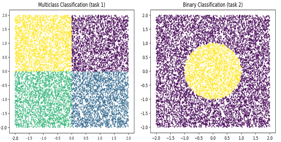
Figure 2: The synthetic dataset $\mathcal{D}$ with respect to its two tasks. Task 1 on the left, task 2 on the right. Different colors denote different labels for the points.

We split $\mathcal{D}$ randomly, so that the training set $\mathcal{T}$, the validation set $\mathcal{V}$, and the test set $\mathcal{P}$ are made of $T=5\,600$ samples, $V=1\,400$ samples, and $P=3\,000$ samples, respectively. Then, we build a MTNN with architecture as described in Table 1 and, both for the classic SG and the implemented ATE-SG procedures, we train it according to the following options:

• Preprocessing: standard scaler for inputs (based on training data only);

• Losses: categorical cross-entropy for task 1, binary cross-entropy (from logits) for task 2, sum of the two losses for the training procedure;

• Optimization hyper-parameters: starting learning rate 0.01, mini-batch size 256, maximum number of epochs $5000$;

• Regularization: early stopping (patience 350, restore best weights), reduce learning rate on plateaus (patience 50, factor 0.75, min-delta $0.0001$);

• Alternate training sub-epochs: $E_{0}=E_{\rm ts}=1,10,100,250$ (for alternate training procedures only).

Layer Name	Layer Type (Keras)	Output Shape	Param. #	Param. # (Grouped)	Connected to
input	InputLayer	(None, 2)	$0$	-	-
trunk_01	Dense (relu)	(None, 512)	$1\,536$	($\boldsymbol{w}_{0}$-param.s)	input
trunk_02	Dense (relu)	(None, 512)	$262\,656$	$526\,848$	trunk_01
trunk_03	Dense (relu)	(None, 512)	$262\,656$		trunk_02
quad_01	Dense (relu)	(None, 512)	$262\,656$	($\boldsymbol{w}_{\rm ts}$-param.s, task 1)	trunk_03
quad_02	Dense (relu)	(None, 512)	$262\,656$	$527\,364$	quad_01
quad_out	Dense (softmax)	(None, 4)	$2\,052$		quad_02
circ_01	Dense (relu)	(None, 512)	$262\,656$	($\boldsymbol{w}_{\rm ts}$-param.s, task 2)	trunk_03
circ_02	Dense (relu)	(None, 512)	$262\,656$	$525\,825$	circ_01
circ_out	Dense (linear)	(None, 1)	$513$		circ_02

Table 1: Synthetic dataset. Keras [7, 2] architecture of the MTNN.

To compare the performance of the different training procedures we first look at the behaviour of the loss functions during the epochs (see Figures 3 and 4), and to the learning rate decay (see Figure 5). In particular, we observe what follows.

Case $E_{0}=E_{\rm ts}=1$. The alternate training procedure appears to have regularization effects on the training in general, which with respect to the classic SG lead to a larger decrease of the loss function and to a marked reduction of its oscillations, on both the training set and the validation set. Such a “smoother” behavior of the validation loss allows to delay the upcoming of the overfitting effect and to improve the generalization abilities of the NN.

Case $E_{0}=E_{\rm ts}=10$. In this case, we see a particular phenomenon: the training results in large, periodic, oscillations for the loss function (both on the training set and the validation set); specifically, these oscillations have a period $E_{0}=E_{\rm ts}$ and are characterized by a range of values much larger than the one of the typical fluctuations characterizing the loss of a classic MTNN training. Nonetheless, the loss on the validation set is still generally decreasing with the epochs; then, also in this case we can observe a phenomenon of “overfitting delay”. In the end, these oscillations tend to disappear when decreasing the learning rate (compare Figures 3 and 4 with Figure 5).

Case $E_{0}=E_{\rm ts}=100,250$. Here, the implemented ATE-SG returns training behaviors very similar to classic SG.

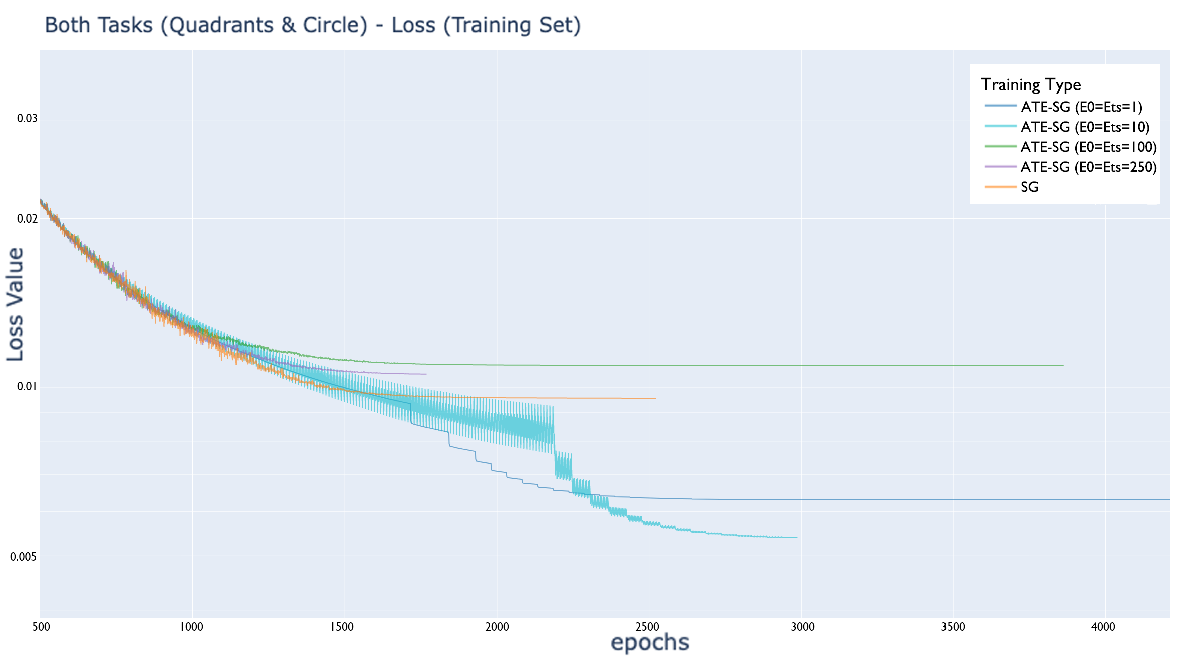
Figure 3: Synthetic dataset. Loss function on the training set (logarithmic scale) during the epochs.

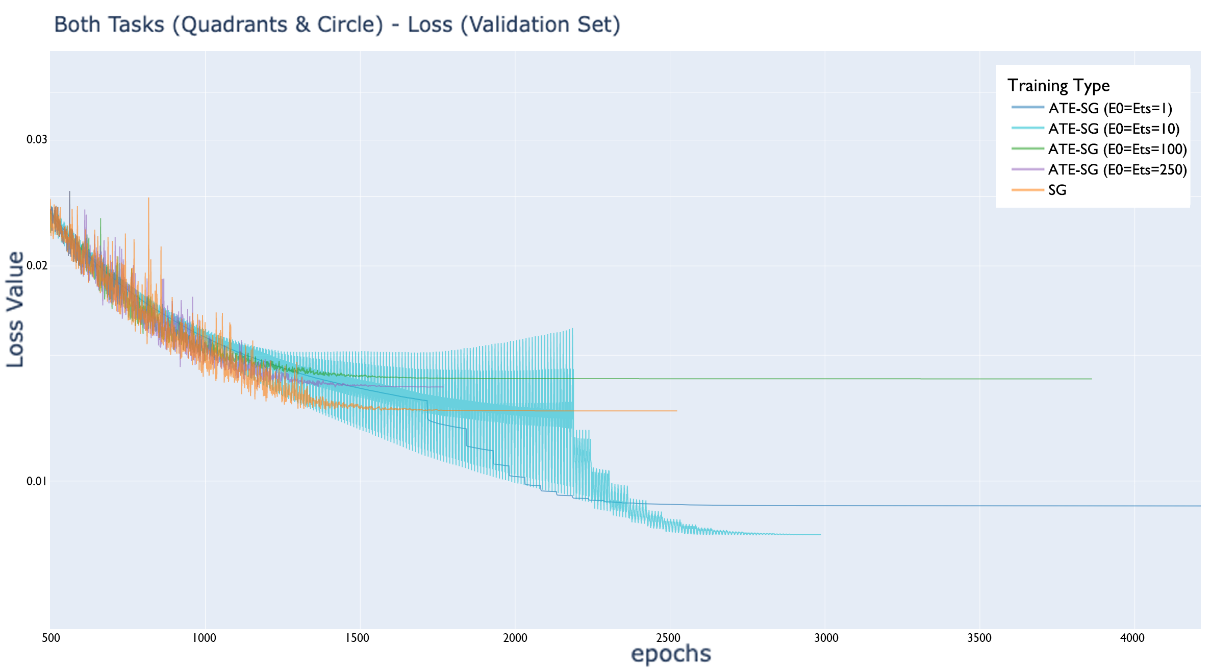
Figure 4: Synthetic dataset. Loss function on the validation set (logarithmic scale) during the epochs.

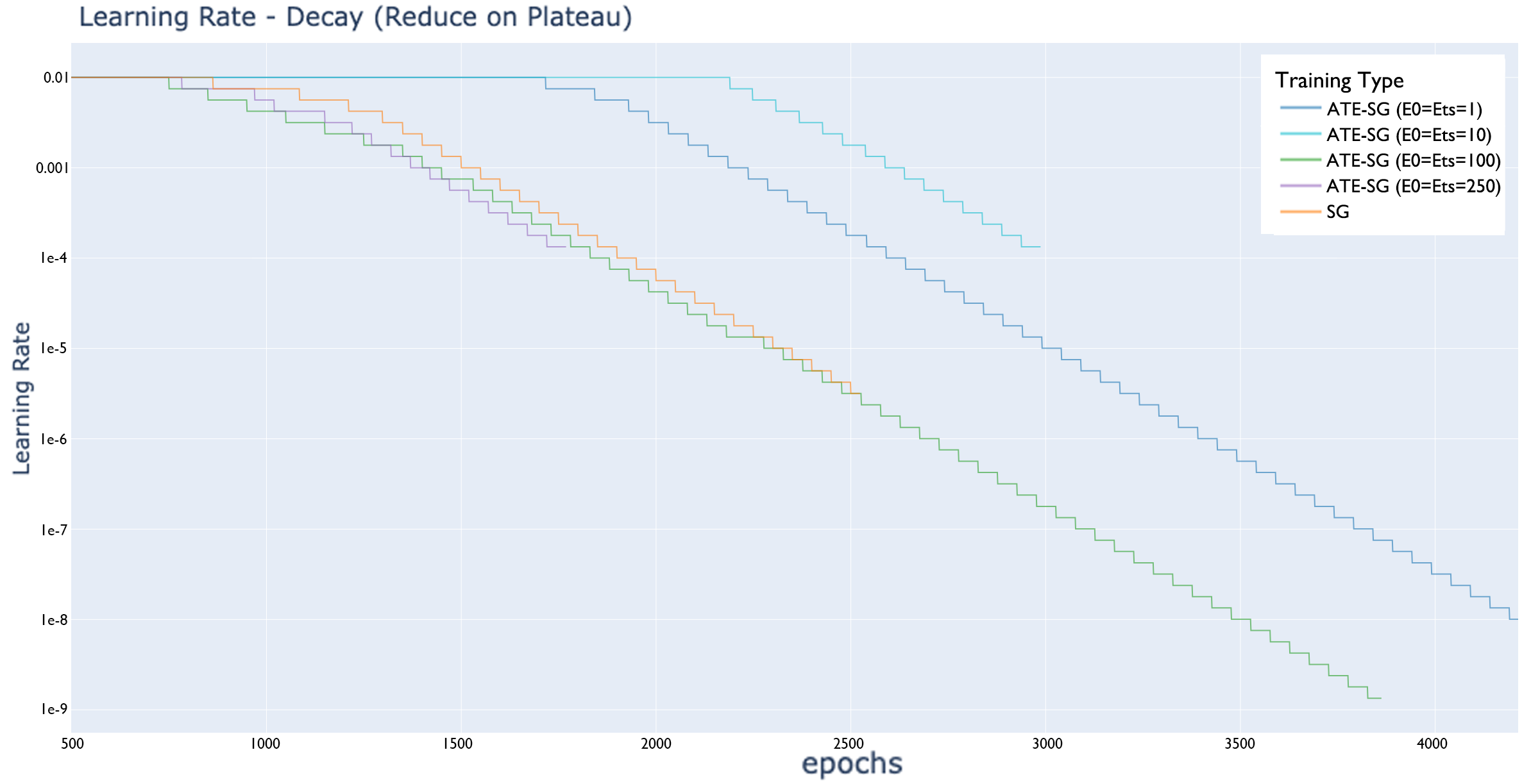
Figure 5: Synthetic dataset. Learning rate decay (logarithmic scale) during the epochs.

Given the observations above, we believe that the implemented ATE-SG method with $E_{0}=E_{\rm ts}=1$ is a good choice for training a MTNN, because the training procedure results to be more regularized and more efficient (see item 1, p.1).

However, from the point of view of the test set performance, for this synthetic dataset we do not observe significant differences between classic or alternate training (see Table 2). Since we are learning classification tasks, performance is measured now through the weighted average precision (in our case equivalent to the accuracy), the weighted average recall, and the weighted average $F_{1}$-score [1]. For more details, see the remark below.

Remark 4.1 (Precision, recall and $F_{1}$-score).

For the reader convenience, we report a brief description of the quantities: precision, recall, and $F_{1}$-score, for each class $C$ of a general classification problem (see [18]). The precision is the percentage of correct predictions among all the elements predicted as $C$; the recall is the percentage of elements predicted as $C$ among all the $C$ elements in the set; the $F_{1}$-score is defined as the weighted harmonic mean of precision and recall. Then, the weighted average precision/recall/$F_{1}$-score is the weighted average of these quantities with respect to the cardinalities of each class in the set. For this reason we have that the weighted average precision is equivalent to the accuracy.

	Accuracy		Recall		$F_{1}$-score
Training Type	task1	task 2	task1	task 2	task1	task 2
ATE-SG ($E_{0}=E_{\rm ts}=1$)	0.999667	0.996997	0.999667	0.997000	0.999667	0.996997
ATE-SG ($E_{0}=E_{\rm ts}=10$)	1.000000	0.997665	1.000000	0.997667	1.000000	0.997664
ATE-SG ($E_{0}=E_{\rm ts}=100$)	0.999000	0.997666	0.999000	0.997667	0.999000	0.997666
ATE-SG ($E_{0}=E_{\rm ts}=250$)	0.999000	0.997666	0.999000	0.997667	0.999000	0.997666
Classic SG	0.999000	0.997999	0.999000	0.998000	0.999000	0.997999

Table 2: Synthetic dataset. Performance of the MTNNs on the test set $\mathcal{P}$.

4.2 Experiments on Real-World Data

For the experiment on real-world data, we report the results obtained on a dataset used for wireless signal recognition tasks [10]. Typically, signal recognition is segmented into sub-tasks like the modulation recognition or the wireless technology (i.e., signal type); nonetheless, in [11, 12] the authors suggest an approach to the problem that exploits a multi-task setting for classifying at the same time both the modulation and the signal type of a wireless signal.

Here we focus on signals characterized by $0{\rm dB}$ Signal-to-Noise Ratio (SNR). The dataset $\mathcal{D}$ is made of $N=63\,000$ signals, each one represented as a vector $\boldsymbol{s}_{i}\in\mathbb{R}^{256}$ obtained from 128 complex samples of the original signal. In the dataset, associated to each signal $\boldsymbol{s}_{i}$, we have a label $\mu_{i}\in\{0,\ldots,5\}$ for the corresponding modulation (task 1) and a label $\sigma_{i}\in\{0,\ldots,7\}$ for the corresponding signal type (task 2). For more details about the data, see [10, 11, 12].

We split $\mathcal{D}$ randomly, so that the training set $\mathcal{T}$, the validation set $\mathcal{V}$, and the test set $\mathcal{P}$ are made of $T=35\,280$ samples, $V=8\,820$ samples, and $P=18\,900$ samples, respectively (i.e., same ratios used for the synthetic data in Section 4.1). Then, we build a MTNN with architecture as described in Table 3 and, both for the classic SG and the implemented ATE-SG procedures, we train it according to the following options:

• Preprocessing: standard scaler for inputs (based on training data only);

• Losses: categorical cross-entropy for both tasks, sum of the two losses for the training procedure;

• Optimization hyper-parameters: starting learning rate 0.001, mini-batch size 512, maximum number of epochs $10000$;

• Regularization: early stopping (patience 350, restore best weights), reduce learning rate on plateaus (patience 50, factor 0.75, min-delta $0.0001$);

• Alternate training sub-epochs: $E_{0}=E_{\rm ts}=1,100$ (for alternate training procedures only).

Due to the larger size of the dataset and the more complex nature of the problem, we decide to reduce the choice for $E_{0}$ and $E_{\rm ts}$ to the set of two values $\{1,100\}$. In particular, we keep the case $E_{0}=E_{\rm ts}=1$ because of the good results observed in the previous experiment; then, we select also $E_{0}=E_{\rm ts}=100$ because it is a large value but sufficiently small, with respect to the the training set cardinality and the mini-batch size, to maintain the characteristics of the alternate training observed in the previous experiment.

Remark 4.2 (MTNN architecture and hyper-parameters).

Since the aim of the experiment is to study how the training performance of a MTNN change when using an alternate training procedure, we do not focus on hyper-parameter and/or architecture optimization for obtaining the best predictions. Then, for simplicity, in this experiment we choose a simple but efficient architecture (see Table 3) based on 1-dimensional convolutional layers, after a brief, manual hyper-parameter tuning. The 1-dimensional convolutional layers are useful to exploit the signals reshaped as 128 complex signals (see layer trunk_00 in Table 3), keeping the NN relatively small.

Layer Name	Layer Type (Keras)	Output Shape	Param. #	Param. # (Grouped)	Connected to
input	InputLayer	(None, 256)	$0$	-	-
trunk_00	Reshape	(None, 128, 2)	$0$		input
trunk_01	Conv1D (relu)	(None, 128, 64)	$576$	($\boldsymbol{w}_{0}$-param.s)	trunk_00
trunk_02	Conv1D (relu)	(None, 128, 32)	$8\,224$	$12\,928$	trunk_01
trunk_03	Conv1D (relu)	(None, 128, 32)	$4\,128$		trunk_02
trunk_end	GlobalMaxPooling1D	(None, 32)	$0$		trunk_03
mod_01	Dense (relu)	(None, 64)	$2\,112$	($\boldsymbol{w}_{\rm ts}$-param.s, task 1)	trunk_end
mod_02	Dense (relu)	(None, 64)	$4\,160$	$6\,662$	mod_01
mod_out	Dense (softmax)	(None, 6)	$390$		mod_02
sig_01	Dense (relu)	(None, 64)	$2\,112$	($\boldsymbol{w}_{\rm ts}$-param.s, task 2)	trunk_end
sig_02	Dense (relu)	(None, 64)	$4\,160$	$6\,792$	sig_01
sig_out	Dense (softmax)	(None, 8)	$520$		sig_02

Table 3: Real-world dataset. Keras [7, 2] architecture of the MTNN.

As we can see from Figures 6-8 and Table 4, the behavior observed in Section 4.1 is somehow preserved and the prediction performance improves evidently for the case $E_{0}=E_{\rm ts}=1$. In particular, we observe the following.

Case $E_{0}=E_{\rm ts}=1$. The regularization effect of this alternate training procedure is much more evident than in the case of Section 4.1, both for the training loss and the validation loss (Figures 6-7). In particular, we see that the upcoming of the overfitting is delayed considerably, without needing to reduce the learning rate for thousands of epochs (Figure 8). We finally stress that, in addition to delay overfitting and then producing a better and more precise training, the alternate procedure with $E_{0}=E_{\rm ts}=1$ provides better prediction performance than training the MTNN with the other two methods (see Table 4), in particular concerning the recall of task1. From another point of view, we can infer that the choice $E_{0}=E_{ts}=1$ yields better training performance than SG or ATE-SG with $E_{0}=E_{\rm ts}=100$, also when using the same, fixed, learning rate.

Case $E_{0}=E_{\rm ts}=100$. In this situation, the alternate training procedure has a behavior similar to both the cases $E_{0}=E_{\rm ts}=10$ and $E_{0}=E_{\rm ts}=100$ of Section 4.1; i.e., it is characterized by large and periodic oscillations of the loss functions, returning a trained NN with approximately the same prediction abilities of the MTNN trained classically. This behavior probably depends on the larger cardinality of both the training set and the mini-batches.

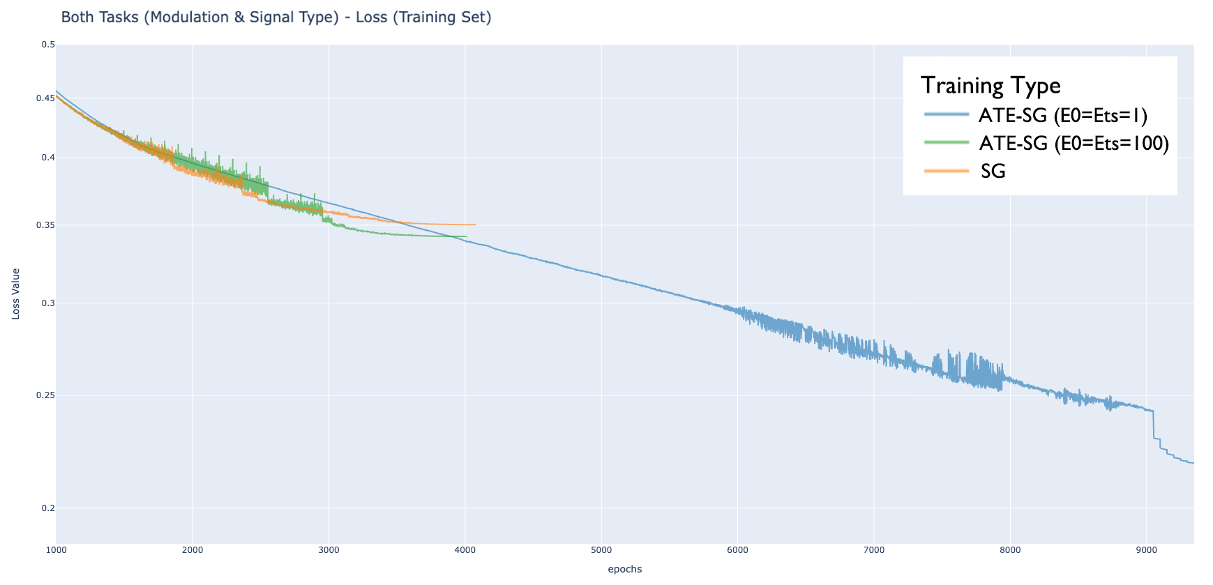
Figure 6: Real-world dataset. Loss function on the training set (logarithmic scale) during the epochs.

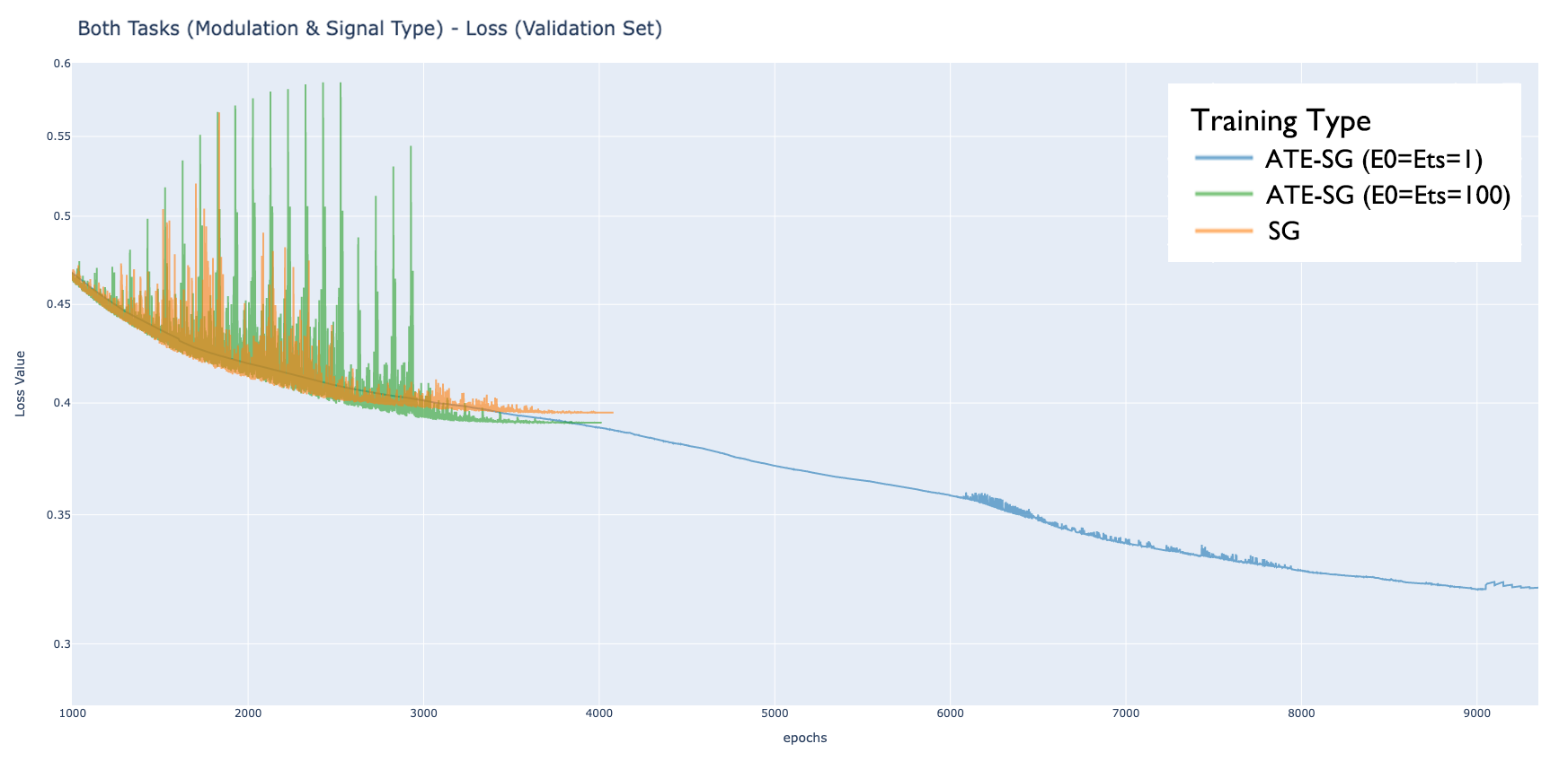
Figure 7: Real-world dataset. Loss function on the validation set (logarithmic scale) during the epochs.

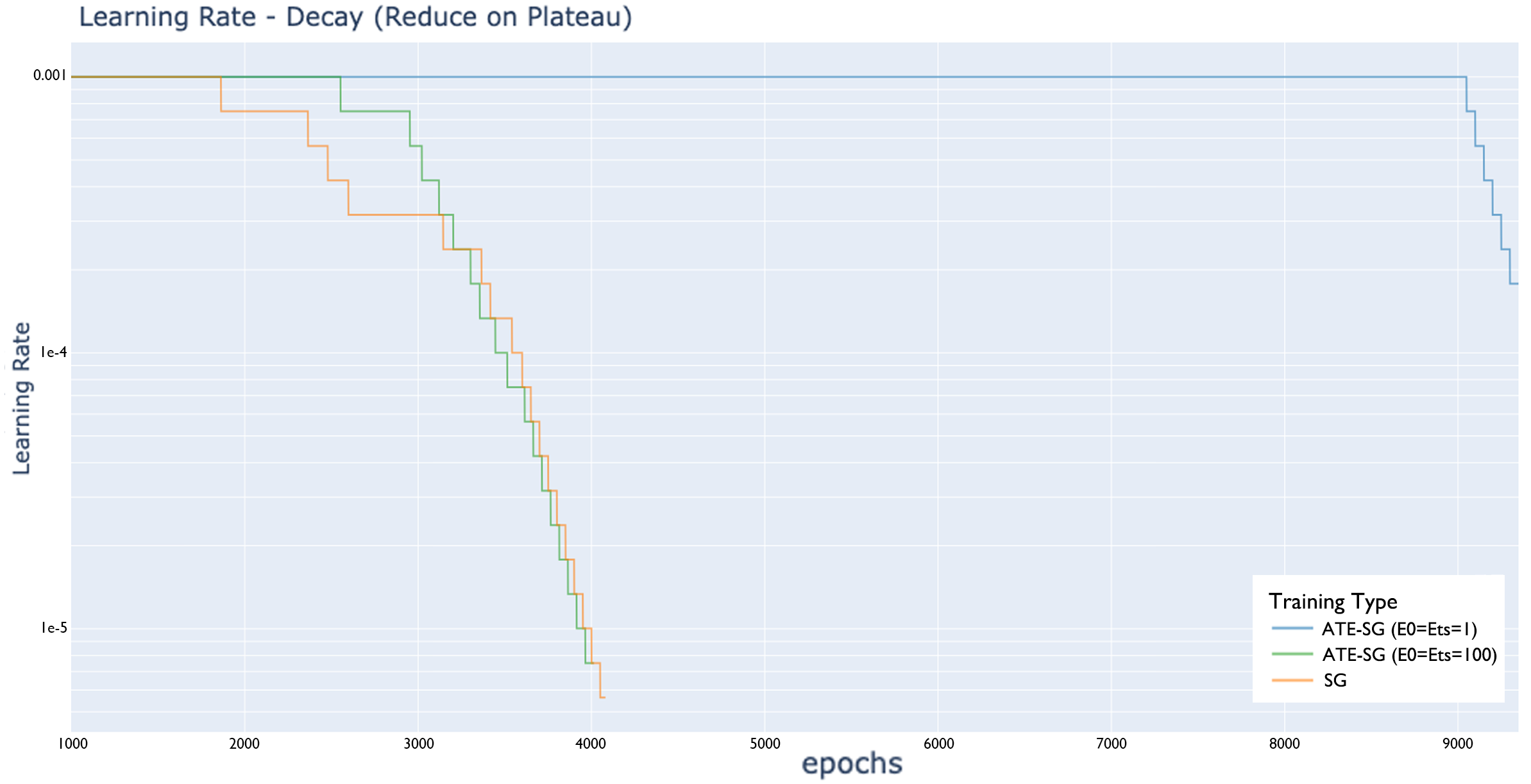
Figure 8: Real-world dataset. Learning rate decay (logarithmic scale) during the epochs.

	Accuracy		Recall		$F_{1}$-score
Training Type	task1	task 2	task1	task 2	task1	task 2
ATE-SG ($E_{0}=E_{\rm ts}=1$)	0.914577	0.960432	0.909471	0.960476	0.909919	0.959814
ATE-SG ($E_{0}=E_{\rm ts}=100$)	0.898932	0.949671	0.861429	0.944656	0.857611	0.940939
Classic SG	0.896005	0.948133	0.855450	0.943862	0.847870	0.940265

Table 4: Real-world dataset. Performance of the MTNNs on the test set $\mathcal{P}$.

Hence the advantages observed in Section 4.1 about training a MTNN by an alternate training procedure with $E_{0}=E_{\rm ts}=1$ are confirmed, showing practical and concrete advantages both from the computational point of view and from the learning point of view (see items 1 and 2, p.1).

5 Conclusion

In this work we presented new alternate training procedures for hard-parameter sharing MTNNs. We started illustrating the properties of the task-specific gradients of the loss function of a MTNN, and explaining the motivations behind the proposed alternate method. Then, in Section 3, we introduced a first formulation of alternate training called Simple Alternate Training (SAT) and a second one called Alternate Training through the Epochs (ATE); both formulations are based on the Stochastic Gradient (SG). For these methods we provided a stochastic convergence analysis (only for SAT, also a deterministic one). We concluded the work illustrating the results of two numerical experiments, where the prediction abilities of a MTNN trained using the implemented ATE-SG algorithm are compared with the prediction abilities of the same MTNN trained using the SG. The experiments show very interesting properties of training the network using the implemented ATE-SG; in particular, we observe a delay in the upcoming of the overfitting, a general improvement of the prediction abilities, and a reduction of the computational costs.

In conclusion, the alternate training procedures presented in this work proved to be a novel and useful approach for training MTNNs. In future work, we will analyze how the procedures may change by replacing the stochastic gradient with other optimization methods.

Appendix A Implemented ATE-SG

The pseudo-code of the implemented ATE-SG method is given in Algorithm 3. For simplicity, we consider the total number of epochs as the only stopping criterion. For a ready-to-use version of this algorithm, see https://github.com/Fra0013To/ATEforMTNN.

Algorithm 3 Implemented ATE-SG

Data:

$(\boldsymbol{w}_{0},\boldsymbol{w}_{\rm ts})=\boldsymbol{w}$ (initial guesses for the trainable parameters), $\mathcal{T}$ (training set), $B$ (mini-batch size), $\{\eta_{i},~{}i\geq 0\}$ (learning rates), $\ell$ (loss function), $E_{0},E_{\rm ts}$ (number of epochs for alternate training), $E$ (total number of epochs).

Procedure:

1:  $\boldsymbol{w}^{(0)}\leftarrow(\boldsymbol{w}_{0},\boldsymbol{w}_{\rm ts})$

2:  $e\leftarrow 0$  (epochs counter, total)

3:  $i\leftarrow 0$  (iteration counter)

4:  while $e\leq E$ do

5:     $e_{0}\leftarrow 0$  (epochs counter, shared phase)

6:     while $e_{0}\leq E_{0}$ and $e\leq E$ (alternate training, shared phase) do

7:        $\{\mathcal{B}_{1},\ldots,\mathcal{B}_{t}\}\leftarrow$ random split of $\mathcal{T}$ into mini-batches w.r.t. $B$

8:        for $\tau=1,2,\ldots,t$ do

9:           $\boldsymbol{w}_{0}\leftarrow\boldsymbol{w}_{0}-\eta_{i}\nabla_{\boldsymbol{w}_{0}}\ell(\mathcal{B}_{\tau};\boldsymbol{w}^{(i)})$

10:           $i\leftarrow i+1$

11:           $\boldsymbol{w}^{(i)}\leftarrow(\boldsymbol{w}_{0},\boldsymbol{w}_{\rm ts})$

12:        end for

13:        $e_{0}\leftarrow e_{0}+1$ and $e\leftarrow e+1$

14:     end while

15:     $e_{\rm ts}\leftarrow 0$  (epochs counter, task-specific phase)

16:     while $e_{\rm ts}\leq E_{\rm ts}$ and $e\leq E$ (alternate training, task-specific phase) do

17:        $\{\mathcal{B}_{1},\ldots,\mathcal{B}_{t}\}\leftarrow$ random split of $\mathcal{T}$ into mini-batches w.r.t. $B$

18:        for $\tau=1,2,\ldots,t$ do

19:           $\boldsymbol{w}_{\rm ts}\leftarrow\boldsymbol{w}_{\rm ts}-\eta_{i}\nabla_{\boldsymbol{w}_{\rm ts}}\ell(\mathcal{B}_{\tau};\boldsymbol{w}^{(i)})$

20:           $i\leftarrow i+1$

21:           $\boldsymbol{w}^{(i)}\leftarrow(\boldsymbol{w}_{0},\boldsymbol{w}_{\rm ts})$

22:        end for

23:        $e_{\rm ts}\leftarrow e_{\rm ts}+1$ and $e\leftarrow e+1$

24:     end while

25:  end while

26:  return  $\boldsymbol{w}^{(i)}$  (final MTNN’s weights)

References

- [1] Scikit-learn. https://scikit-learn.org. Accessed on: 2023-09-09.
- [2] M. Abadi, A. Agarwal, P. Barham, E. Brevdo, Z. Chen, C. Citro, G. S. Corrado, A. Davis, J. Dean, M. Devin, S. Ghemawat, I. Goodfellow, A. Harp, G. Irving, M. Isard, Y. Jia, R. Jozefowicz, L. Kaiser, M. Kudlur, J. Levenberg, D. Mané, R. Monga, S. Moore, D. Murray, C. Olah, M. Schuster, J. Shlens, B. Steiner, I. Sutskever, K. Talwar, P. Tucker, V. Vanhoucke, V. Vasudevan, F. Viégas, O. Vinyals, P. Warden, M. Wattenberg, M. Wicke, Y. Yu, and X. Zheng, TensorFlow: Large-scale machine learning on heterogeneous systems, 2015, https://www.tensorflow.org/. Software available from tensorflow.org.
- [3] D. Bertsekas, Nonlinear Programming, Athena scientific optimization and computation series, Athena Scientific, 1999, https://books.google.it/books?id=TgMpAQAAMAAJ.
- [4] L. Bottou, F. E. Curtis, and J. Nocedal, Optimization methods for large-scale machine learning, SIAM Review, 60 (2018), pp. 223–311, https://doi.org/10.1137/16M1080173, https://doi.org/10.1137/16M1080173, https://arxiv.org/abs/https://doi.org/10.1137/16M1080173.
- [5] F. Bragman, R. Tanno, S. Ourselin, D. Alexander, and J. Cardoso, Stochastic filter groups for multi-task cnns: Learning specialist and generalist convolution kernels, in 2019 IEEE/CVF International Conference on Computer Vision (ICCV), 2019, pp. 1385–1394, https://doi.org/10.1109/ICCV.2019.00147.
- [6] Z. Chen, V. Badrinarayanan, C.-Y. Lee, and A. Rabinovich, GradNorm: Gradient normalization for adaptive loss balancing in deep multitask networks, in Proceedings of the 35th International Conference on Machine Learning, J. Dy and A. Krause, eds., vol. 80 of Proceedings of Machine Learning Research, PMLR, 10–15 Jul 2018, pp. 794–803, https://proceedings.mlr.press/v80/chen18a.html.
- [7] F. Chollet et al., Keras. https://keras.io, 2015.
- [8] R. Cipolla, Y. Gal, and A. Kendall, Multi-task learning using uncertainty to weigh losses for scene geometry and semantics, in 2018 IEEE/CVF Conference on Computer Vision and Pattern Recognition, 2018, pp. 7482–7491, https://doi.org/10.1109/CVPR.2018.00781.
- [9] M. Guo, A. Haque, D.-A. Huang, S. Yeung, and L. Fei-Fei, Dynamic task prioritization for multitask learning, in Computer Vision – ECCV 2018, V. Ferrari, M. Hebert, C. Sminchisescu, and Y. Weiss, eds., Cham, 2018, Springer International Publishing, pp. 282–299.
- [10] A. Jagannath and J. Jagannath, Dataset for modulation classification and signal type classification for multi-task and single task learning, Computer Networks, 199 (2021), p. 108441, https://doi.org/10.1016/j.comnet.2021.108441, https://doi.org/10.1016/j.comnet.2021.108441.
- [11] A. Jagannath and J. Jagannath, Multi-task Learning Approach for Automatic Modulation and Wireless Signal Classification, in Proc. of IEEE International Conference on Communications (ICC), Montreal, Canada, June 2021.
- [12] A. Jagannath and J. Jagannath, Multi-task Learning Approach for Automatic Modulation and Wireless Signal Classification, IEEE International Conference on Communications, (2021), https://doi.org/10.1109/ICC42927.2021.9500447, https://arxiv.org/abs/2101.10254.
- [13] I. Kokkinos, Ubernet: Training a universal convolutional neural network for low-, mid-, and high-level vision using diverse datasets and limited memory, in Proceedings of the IEEE Conference on Computer Vision and Pattern Recognition (CVPR), July 2017.
- [14] H. Liu, M. Palatucci, and J. Zhang, Blockwise coordinate descent procedures for the multi-task lasso, with applications to neural semantic basis discovery, in Proceedings of the 26th Annual International Conference on Machine Learning, ICML ’09, New York, NY, USA, 2009, Association for Computing Machinery, p. 649–656, https://doi.org/10.1145/1553374.1553458, https://doi.org/10.1145/1553374.1553458.
- [15] S. Liu and L. Vicente, The stochastic multi-gradient algorithm for multi-objective optimization and its application to supervised machine learning, Annals of Operations Research, (2021), https://doi.org/10.1007/s10479-021-04033-z, https://doi.org/10.1007/s10479-021-04033-z.
- [16] S. Liu and L. Vicente, Accuracy and fairness trade-offs in machine learning: a stochastic multi-objective approach, Computational Management Science, 19 (2022), pp. 513–537, https://doi.org/10.1007/s10287-022-00425-z, https://doi.org/10.1007/s10287-022-00425-z.
- [17] S. Liu and L. Vicente, Convergence Rates of the Stochastic Alternating Algorithm for Bi-Objective Optimization, Journal of Optimization Theory and Applications, 198 (2023), pp. 165–186, https://doi.org/10.1007/s10957-023-02253-w, https://doi.org/10.1007/s10957-023-02253-w.
- [18] J. Makhoul, F. Kubala, R. Schwartz, and R. Weischedel, Performance measures for information extraction, in Proceedings of DARPA Broadcast News Workshop, 1999.
- [19] K.-K. Maninis, I. Radosavovic, and I. Kokkinos, Attentive single-tasking of multiple tasks, in 2019 IEEE/CVF Conference on Computer Vision and Pattern Recognition (CVPR), 2019, pp. 1851–1860, https://doi.org/10.1109/CVPR.2019.00195.
- [20] Q. Mercier, F. Poirion, and J. Désidéri, A stochastic multiple gradient descent algorithm, European Journal of Operational Research, 271 (2018), pp. 808–817, https://doi.org/https://doi.org/10.1016/j.ejor.2018.05.064, https://www.sciencedirect.com/science/article/pii/S0377221718304831.
- [21] A. Navon, A. Shamsian, I. Achituve, H. Maron, K. Kawaguchi, G. Chechik, and E. Fetaya, Multi-Task Learning as a Bargaining Game, in Proceedings of the 39th International Conference on Machine Learning, vol. 162, 2022, https://doi.org/https://doi.org/10.48550/arXiv.2202.01017.
- [22] L. Pascal, P. Michiardi, X. Bost, B. Huet, and M. A. Zuluaga, Improved optimization strategies for deep Multi-Task Networks, arXiv preprint, (2021), https://doi.org/https://doi.org/10.48550/arXiv.2109.11678.
- [23] H. Robbins and D. Siegmund, A Convergence Theorem for Non Negative Almost Supermartingales and some Applications, in Optimizing Methods in Statistics, J. S. Rustagi, ed., Academic Press, 1971, pp. 233–257, https://doi.org/https://doi.org/10.1016/B978-0-12-604550-5.50015-8, https://www.sciencedirect.com/science/article/pii/B9780126045505500158.
- [24] G. Strezoski, N. v. Noord, and M. Worring, Many task learning with task routing, in Proceedings of the IEEE/CVF International Conference on Computer Vision (ICCV), October 2019.
- [25] M. Teichmann, M. Weber, M. Zollner, R. Cipolla, and R. Urtasun, Multinet: Real-time joint semantic reasoning for autonomous driving, (2018), https://doi.org/10.17863/CAM.26778, https://www.repository.cam.ac.uk/handle/1810/279403.
- [26] S. Vandenhende, S. Georgoulis, W. Van Gansbeke, M. Proesmans, D. Dai, and L. Van Gool, Multi-task learning for dense prediction tasks: A survey, IEEE Transactions on Pattern Analysis and Machine Intelligence, 44 (2022), pp. 3614–3633, https://doi.org/10.1109/TPAMI.2021.3054719.
- [27] Y. Zhang and Q. Yang, A survey on multi-task learning, IEEE Transactions on Knowledge and Data Engineering, 34 (2022), pp. 5586–5609, https://doi.org/10.1109/TKDE.2021.3070203.