Mathematical LoRE: Local Recovery of Erasures using Polynomials, Curves, Surfaces, and Liftings ††thanks: Haymaker is with the Department of Mathematics and Statistics, Villanova University (email: kathryn.haymaker@villanova.edu). López and Matthews are with the Department of Mathematics, Virginia Tech (email: {hhlopez, gmatthews}@vt.edu). Malmskog is with the Department of Mathematics & Computer Science, Colorado College (email: bmalmskog@coloradocollege.edu). Piñero is with the Department of Mathematics, University of Puerto Rico - Ponce (email: fernando.pinero1@upr.edu). The National Science Foundation partially supported the second (DMS-2201094 and DMS-2401558), third (DMS-2137661), and fourth (DMS-2201075) authors. The fourth author is also partially supported by the Commonwealth Cyber Initiative. The team acknowledges support from the American Institute of Mathematics SQuaRES program.
Abstract
Employing underlying geometric and algebraic structures allows for constructing bespoke codes for local recovery of erasures. We survey techniques for enriching classical codes with additional machinery, such as using lines or curves in projective space for local recovery sets or products of curves to enhance the availability of data.
I Introduction and Motivation
Algebraic, geometric, and combinatorial structures have long supported the development of codes for error correction and erasure recovery in which these mathematical structures guarantee the desired properties of the code. Prime examples are Reed-Solomon codes [20], in which codewords are defined by evaluating polynomials of bounded degree at elements of a finite field. Reed-Solomon codes have seen widespread use since their introduction in 1960, from satellite communications to QR codes. However, the code length is bounded by the alphabet size, meaning no nontrivial binary Reed-Solomon codes exist. The desire to decouple the code length and alphabet size is natural, especially when combined with the search for long codes inspired by Shannon’s Theorem. This aspiration led to the breakthrough construction of algebraic geometry codes in the 1970s by V. D. Goppa [7]. Algebraic geometry codes are built from curves or higher-dimensional varieties over finite fields, which can have more rational points than the field size, leading to codes that can be much longer than Reed-Solomon codes over the same field. The underlying vector spaces of functions gave rise to codes with exceptional parameters, including those exceeding the Gilbert-Varshamov bound [26]. Refinements of these structures can lead to codes amenable to the local recovery of erased data.
Traditionally, the decoder takes a received word as input and attempts to correct any errors or recover any erasures introduced during the transmission. This classical scenario assumes access to the entire received word. Distributed networks, cloud storage, and blockchains are formed from hundreds or thousands of servers. So, it is impractical to assume access to all coordinates of the received word in the decoding process. Hence, it is desirable to design codes that can recover a few codeword symbols by accessing only a few other symbols of the received word. Such a code is called a locally recoverable code, or LRC.
LRCs provide smart data storage across a network with limited recovery and repair traffic. A small recovery set reconstructs unavailable or lost symbols. The rich underlying mathematical structures that gave the world Reed-Solomon codes and their higher-genus relatives (algebraic geometry codes) aid in the design of LRCs. In Section II, we review some algebraic and geometric structures and how they define LRCs.
One might set various objectives while considering codes for local recovery. One goal is to have different (often many) disjoint recovery sets to ensure high data availability. Thus, even with multiple erasures, there is a recovery set with enough data to recover the missing symbol(s). The availability measures the largest number of disjoint recovery sets for all coordinates. We will see rich structures that give rise to codes with availability in Section III.
Another objective is to minimize the size of the largest recovery set - called the locality of the code - to reduce the network traffic involved in recovering a failed node or erasure. It is natural to ask if these codes are MDS or meet other classical bounds. Of course, the additional structure required on a classical code to achieve local recovery can adversely impact the code’s overall efficiency and error-correcting capability. For this reason, while traditional bounds for error-correcting codes apply to locally recoverable codes, they are not tight. Instead, bounds for LRCs take into account locality. These bounds are discussed in Section IV. A conclusion may be found in Section V.
II Algebraic and Geometric Tools
An approach to developing an LRC is to add an underlying algebraic or geometric structure to a classical code. These structures allow additional machinery, such as the trace function of an extension field to minimize data transmission, lines or curves in the projective space to create recovery sets, or products of curves to enhance availability. Polynomials, curves over finite fields, and other algebraic or algebraic geometric objects have a long history in coding theory. We will use standard coding theory notation throughout, working over the finite field with elements. An code over the alphabet is a -dimensional -subspace of such that any two different elements (called codewords) differ in at least coordinates.
Consider a vector space of -valued functions and points on a geometric object so that for all for all functions in . We will consider evaluation codes
where ; that is, where
We recognize this construction giving rise to important families of codes:
-
•
Taking positive integers , , the set of polynomials with coefficients in of degree less than , and , is the Reed-Solomon code over .
-
•
Setting and taking to be the set of polynomials with coefficients in of total degree less than gives a Reed-Muller code.
-
•
Considering -rational points on a curve over and a divisor with support not containing any allows one to define an algebraic geometry code by taking .
We will see that fine-tuning the design choices and allow local recovery of erased data.
Definition 1.
A code has locality if for each codeword coordinate , there exists a set of other coordinates such that for all , for some function and . The set (resp., ) is called a recovery set (resp., repair group) for .
Because any code has locality , we are interested in codes with locality . The following Singleton-type bound describes the relationship between the standard code parameters (length, dimension, and minimum distance) and the locality for a linear code [6]; a version for nonlinear codes is given in [18].
Theorem 2.
The parameters of an LRC with locality satisfy
| (1) |
If has parameters meeting Bound (1), we say that is an optimal LRC. It is immediate that the Bound (2) reduces to the Singleton bound when considering an code to have locality .
Next, we will meet some families of LRCs, one from polynomials and another from curves, some of which are optimal (see Section IV).
II-A Locally recoverable codes from polynomials
To construct a polynomial LRC, we first consider evaluation codes, similar to Reed-Solomon codes, that rely on a particular polynomial set known as good polynomials. Fix integers with and . The latter condition may be dropped, but we keep it for the convenience.
Definition 3.
A polynomial is said to be good if and there exists a partition of ,
with parts satisfying for every and for all .
The idea is that a good polynomial reduces to a constant on each part of , so each of these parts forms a repair group. Tamo and Barg used good polynomials in [23] to define optimal polynomial LRCs. Rather than evaluating all polynomials of bounded degree, as in the Reed-Solomon case, the functions that give rise to codewords in a polynomial LRC are elements of
The polynomial LRC is , meaning
Notice that every in can be written as for some . This expression allows for local recovery of an erased coordinate as follows. Suppose . Since is a good polynomial, for some for all . Hence, the polynomial , when restricted to , is
a polynomial of degree at most . Then can be determined using values via interpolation, so that the value is found. In [23], it is shown that is an code, making it an optimal LRC. This construction depends on the existence of good polynomials. We will see an example and then discuss some sources of them.
Example 4.
Consider , the nonzero elements of . Take , so . Notice that
Set and Then
Here,
The code can recover any symbol using only 2 symbols , where . For instance, suppose
is received from sent , meaning is erased and , as shown in Figure 1.
To recover the symbol , we may use and . The unique polynomial of degree such that and is
Then, the lost symbol is
which is recovered using only two symbols rather than six required by a Reed-Solomon code of the same dimension.
Example 4 demonstrates how a good polynomial aids in local recovery, raising the question of how one finds good polynomials. Given a subgroup of , the polynomial is a good polynomial with respect to the partition given by the cosets of [23, Proposition 3.2]. In [17], Micheli demonstrates a Galois theoretical approach that explicitly constructs good polynomials. The key idea is that the number of partitions is linked to the number of totally split places of degree in , where is transcendental and is a zero of in the algebraic closure of .
This idea of functions that reduce to low-degree polynomials is a theme throughout the algebraic constructions of LRCs. Next, we will see how curves over finite fields construct longer LRCs.
II-B Locally recoverable codes from curves
As described in the previous subsection, a major contribution of Tamo and Barg is that one can carefully create spaces of one-variable polynomials, including those of high-degree, so that each element of the evaluation set has a small helper set, on which these functions restrict to low-degree polynomials that can be interpolated using the helper set. In 2015, Tamo, Barg, and Vladut extended this idea to functions of more variables, evaluated them at selected points on a curve in a higher-dimensional space [3]; also see [4]. The most basic version begins with a plane curve , defined by the vanishing of some polynomial . Concretely, points on are pairs so that . There may also be points at infinity, but for simplicity, we focus on the affine (non-infinite) points in this article. Much like one could consider complex solutions to an equation with real coefficients, one may look for points on in any larger field containing , and the set of points over a field is specified by .
To capture the intuition of the Tamo-Barg-Vladut construction, we begin with an illustrative example from [4]. Consider the Hermitian curve defined by the equation . We consider . Note that is the field trace function that is a -to-one map . Also, is the field norm function that is a -to-one map . For any , there are -values and -values in with . When , we still have -values but only a single -value so that . Counting the possibilities, there are solutions to this equation over the field . For example, when , we find 27 solutions to , where .
The Hermitian curve has been well-studied by mathematicians and coding theorists. It is particularly interesting in coding theory because it is a maximal curve, having as many points as mathematically possible for a curve of its complexity. Consider the set of functions on defined by
where is a parameter that can be increased for a larger rate and decreased for a larger minimum distance in the final code. Let be the set of all affine points. Barg, Tamo, and Vladut showed that the evaluation code is locally recoverable and determined its parameters.
To see that we have local recovery, consider the projection of points in to their -coordinate. Say . Then is the set of all points on with -coordinate . As above, there are different -values over so that , so . We let
be the recovery set for the -th position in the code, corresponding to point . Since all the members of have , any will act as a single variable polynomial on . The degree of is at most by construction, so the value of can be interpolated from the values of for the -elements of .
Continuing the example on , we will choose , yielding
a vector space of dimension 6. For any -value in , there are 3 -values in with . For each of the three points , the recovery set for the position corresponding to one point is the positions of the other two points with . Thus, we have an LRC with , , and .
To state a more general construction, we introduce a little notation. One may define a field of rational functions on the points of defined over , denoted . Each function in has a representative ; two functions represent the same function in if for some .
Given two curves and , a morphism is a function defined by polynomials in so that . If such a map exists, we call a cover of by . Given a function , also defines a function on by composition with . Thus there is a natural inclusion . According to the primitive element theorem, we know that there is some so that , where there is some algebraic relation between and the elements of . Barg, Tamo, and Vladut’s key observation was that we may create a locally recoverable code from any such covering of curves.
Let be the degree of the map . Let such that, for each ,
i.e. each point in has a full fiber in the map , with all points in the fiber defined over . We then define to be the evaluation set for our code. Let be a basis for an -dimensional linear space of functions in having no poles in . Let
an -vector space of functions defined on . The evaluation code is a locally recoverable code of dimension and locality . Local recovery is accomplished as follows. Let , with . Let
We have that for all and all . Let . Imagine that position is erased from the corresponding codeword . We want to recover the value using the recovery set . We observe that is a polynomial in of degree at most . Thus can be interpolated from the value of on the points in .
Example 5.
Let
be the Hermitian curve and
its quotient over and the degree morphism
Then is a code with locality . If we take instead , adjusting the morphism accordingly, we obtain a with locality . Using , we obtain a code with locality .
This construction is remarkable in its flexibility, allowing LRCs with a wide range of localities to be constructed. Further, we see here an exciting application of algebraic-geometric structure and relationships to obtain desirable structures in codes. The Tamo-Barg polynomial LRCs described in the previous subsection are subcodes of Reed-Solomon codes, with length limited by field size. By employing curves over finite fields, this construction allows for long evaluation-based LRCs to be constructed over smaller fields. In particular, we see that the length of codes defined over from this construction can be up to where is the genus of the curve .
III Availability
Locally recoverable codes are motivated by applications that are especially relevant in distributed storage, where servers will fail, and the information of a codeword symbol must be recovered from the remaining servers. However, it may be the case that a particular codeword symbol is simply in high demand and therefore unavailable because of increased traffic. Locally recoverable codes allow more users to access this symbol through its recovery set. If the symbol is in extremely high demand, it may be helpful to have additional disjoint recovery sets. This motivates the notion of availability in LRCs.
Definition 6.
A locally recoverable code is said to have availability and locality if each codeword position has disjoint local recovery sets, with the -th repair set for each position having a size at most . Such a code is called an LRC().
Locally recoverable codes with high availability are also exciting from a theoretical computer science perspective. LRC()s with are equivalent to locally decodable codes (LDCs) and have applications in private information retrieval and cryptography.
There are several approaches to constructing codes with availability by patching together LRCs. For example, one can take a combinatorial approach, as in the product code arising from binary parity check codes suggested by Tamo and Barg in [22]. Geometric constructions have again been extraordinarily useful in producing LRC()s through natural geometric structures. We discuss two major approaches here.
III-A Codes from fiber products
We return now to the LRCs from covering maps of algebraic curves discussed in Section II-B. In this setting, locality arises from fibers in a covering map of curves. To obtain availability, it would be useful to have a single curve with several covering maps to other curves, each of which would create a disjoint recovery set to each point. In fact, an algebraic-geometric construction gives exactly such a curve, the fiber product. Since these constructions and theorems are somewhat technical when stated in full generality, we omit the statements in favor of intuition and motivation. Intuitively, given curves , each of which equipped with a covering map to another curve
we can construct a curve as the product of these curves, which will have the desired covering map such that for all . We denote the fiber product by
and set . The fiber product of curves is a curve that can be considered a generalized intersection of hypersurfaces defined by the equations for the curves in a higher-dimensional space. Fiber products can be viewed abstractly from a category or scheme-theoretic perspective. However, there is no need for advanced machinery to work with these objects. The points of are just tuples of points in the Cartesian product
such that
The fiber product can create a “custom” curve, which is equipped with maps arising from the projections . It is one natural extension of the Barg, Tamo, Vladut construction of LRCs from covering maps of curves to LRC()s. In fact, these authors described the idea, gave parameter bounds, and constructed examples of LRC()s from fiber products in [4]. Haymaker, Malmskog, and Matthews extended the construction to LRC()s in [11], giving a slightly improved minimum distance.
Here, we consider some instances of well-known fiber products that yield codes with availability. The first one provides availability two, and the second yields an arbitrary availability. Both are from families of curves with “built-in” recovery sets satisfying the disjoint repair property arising from factors in the fiber product.
III-A1 Generalized Giulietti-Korchmaros (GK) curves
Consider the generalized Giulietti-Korchmaros curve over for an integer , which is the fiber product over of two curves:
The number of -rational points on is
We can take to be the natural degree projection map onto the coordinate for affine points, with and be the natural degree projection map onto the coordinate for affine points, with . One may verify that this design gives rise to two disjoint recovery sets for each coordinate: one of size and another with elements. Even though the projections and hark back to the constructions using covers, since they arise from the fiber product, the recovery sets produced are disjoint. That would not typically occur if one begins with a curve and projects onto different curves and .
Example 7.
Consider the generalized Giulietti-Korchmaros curve over as pictured in Figure 2. Here, and , and is the fiber product over of two curves:
There number of -rational points on is
of which are evaluation points for the code. The recovery sets are based on maps and , the natural degree and degree projection maps mapping infinite points on and to , the point at infinity on . This setting gives rise to codes of length in which each coordinate has two disjoint recovery sets: one of cardinality and the other of cardinality . The dimension can be tailored to any value
by choosing a positive integer , in which case we take
For instance, setting gives a code over , which has localities and .
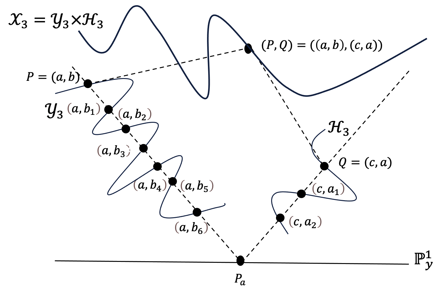
In particular, consider the point on where is a point on and is a point on as shown in Figure 3. Then an erasure at can be recovered using either the coordinates indexed by the set
or by the set
As in this example, the generalized Giulietti-Korchmaros curves naturally yield availability , meaning locally recoverable codes with two disjoint recovery sets for each symbol, one from each factor in the fiber product.
III-A2 Artin-Schreier curves
To design for a particular availability , one may use a family of maximal curves which are fiber products of Artin-Schreier curves (themselves maximal curves) as studied by van der Geer and van der Vlugt [27].
III-B Lifted codes
Polynomial LRCs and LRCs from curves have a key idea in common: restriction or projection naturally gives rise to recovery sets. Liftings, introduced by Guo, Kopparty, and Sudan [8], suggest another approach using curves to design LRCs with availability. The idea is to choose a short code (for example, a Reed-Solomon code) and define a longer code by requiring that all codewords in the longer code restrict to codewords of the short code (on particular subsets). One version of this extends a Reed-Muller code with multivariate polynomials of total degree at most over by adding all polynomials which restrict to single variate polynomials of degree at most on every line. The surprising insight of Guo, Kopparty, and Sudan is that adding these polynomials dramatically increases the code rate, yielding LRCs with high availability and good rates. This idea has been adapted to the Hermitian curves to yield Hermitian-lifted codes defined in [14]. With Hermitian-lifted codes, intersections of lines and curves provide a high rate and high availability via algebraic-geometric constructions, which we will describe now. The choice of lines rather than quadratics or higher degree curves is intentional, motivated by the need for disjoint recovery sets. Because any two lines and intersect in at most a single point , choosing points from and as recovery sets allows them to be naturally disjoint.
We return to the Hermitian curve to describe the construction, though other curves have been explored similarly. To build high-rate codes, codewords are defined using a carefully curated, as-large-as-possible set of rational functions from among the rational functions on the Hermitian curve , in particular, those that restrict to low-degree polynomials on the intersections of the lines and the curve . Let with , with .
Example 8.
Consider the Hermitian curve over and the line with nonzero . Then the rational function given by the monomial restricted to the line is
according to the Freshman’s Dream. While at first glance, it appears that , further reduction is possible using the equation of the curve and the fact that
for all points on both the line and the curve . In fact, in [14], it is shown that . Functions that reduce in such a way are the inspiration for Hermitian-lifted codes.
The set of all non-horizontal lines is
To consider which functions restrict to low-degree polynomials on the line , we consider functions modulo
and to mean .
Definition 9.
The Hermitian-lifted code is , where
is the sum of -rational points on other than , and . Elements of are called good for .
Due to the underlying geometry of the Hermitian curve, any non-horizontal line through intersects in other -points. Each collection of such points acts as a recovery set for the coordinate associated with . Moreover, there are such lines, one for each . It is then easy to see that the Hermitian-lifted code over has length , locality , and availability .
Analyzing these lifted codes depends largely on understanding , the set of functions that restrict to polynomials of degree at most on the curve. Recall the set of functions on with no poles other than is spanned by
Certainly, provided , but it turns out that there are many more functions. To get a handle on which rational functions are elements of , for a polynomial , define
the remainder resulting upon division of by , and set . Then
for all . We say that a monomial is good for if for all lines with ,
Certainly, monomials with are good. In addition, some monomials with are also good, namely those that happen to reduce to those of degree less than the locality on all lines; they are called sporadic.
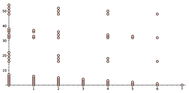
Example 10.
Consider the Hermitian curve over , which has 512 rational points other than the point at infinity, giving a code of length . The monomials with are good for . One may also calculate sporadic good monomials using [25]. The exponent vectors satisfying this condition form a triangle as shown in Figure 4.
While computational tools such as [25] may be used to determine the sporadic monomials for particular values of , combinatorial methods are needed for general . Applying Lucas’s Theorem as in [14, Theorem 10], we see that with , , such that there exists , so that with , , and no term in binary expansions of and is a sporadic monomials. This observation allows one to prove the following.
Theorem 11.
Suppose that is a power of . Then the Hermitian lifted code is a code of length , locality , availability , and rate of at least .
Example 12.
Continuing Example 10, we see that Theorem 11 indicates that the code has dimension 75, with basis the set of monomials plotted in Figure 4. In contrast, the comparable non-lifted one-point Hermitian code has dimension 36, making the rate of the Hermitian-lifted code at least whereas the rate of the comparable one-point code is .
Generalizing the Hermitian-lifted code construction to other curves can be a worthwhile but delicate process. We consider binary norm-trace lifted codes, as in [16], to see that. The norm-trace curve over is
meaning the norm of is the trace of where both the norm and the trace are taken relative to the extension . Taking gives the Hermitian curve over . The norm-trace curve over has rational points other than the point at infinity.
To mimic the Hermitian-lifted code construction for the norm-trace curve, one must determine the cardinalities of the intersections of lines with points on the curve. Restricting to the case , we see
| (2) |
for all lines [16, Lemma 1]. Hence, any non-horizontal lines through an evaluation point intersect in at least other -rational points. This allows for locality and recovery sets for each coordinate. To define the binary-norm-trace lifted code, we need the appropriate set of functions, described next.
Definition 13.
The binary norm-trace-lifted code is where
is the sum of -rational points on other than , and .
Theorem 14.
Suppose that is a power of . Then the binary norm-trace-lifted code is a code of length , locality , availability with an asymptotic rate of .
| () | Norm-trace code | HLC | NTLC |
|---|---|---|---|
| Field size | |||
| Locality | |||
| Availability | |||
| Length | |||
| Dimension |
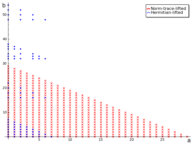
It is natural to consider comparisons between the lifted constructions using the Hermitian and norm-trace codes. Table I highlights the larger relative locality of the norm-trace-lifted codes, which might not be desirable, given that a larger percentage of coordinates are involved in local recovery than in the comparable Hermitian case. Even so, there is an upside. The greater locality means a more controlled set of good monomials, as seen in Figure 5.
IV Bounds and Some Optimal Constructions
The classical MDS bound states that for an code, . When locality is taken into account, the bound was refined to as in Theorem 2.
Note that the polynomial LRCs with alphabet have length at most . In contrast, longer LRCs from curves are possible but not optimal. It is natural to wonder if optimal LRCs are short. This question is reminiscent of the MDS conjecture for linear codes, prompting an interesting line of work resulting in optimal LRCs of lengths [12] using elliptic curves and [13] using automorphism groups.
When equality is attained in codes without locality, the length is bounded by the alphabet size ( for some cases when is even). However, when considering optimal codes with locality, the length can be much larger than the alphabet size. For example, Luo, Xing, and Yuan proved in [15] that optimal LRCs of any length for exist. Moreover, in [10], Guruswami, Xing, and Yuan showed that if , optimal LRCs have length at most . If , then optimal LRCs have length at most .
For LRCs with availability , an analog to the Singleton bound is:
| (3) |
which was introduced in [28] for linear codes and proved in [19] for linear and nonlinear codes in which every information symbol has disjoint repair groups. In [28], Wang and Zhang construct optimal linear LRC()s for . In general, it is an open question whether Bound (3) is tight, and the project of constructing optimal LRC()s is ongoing. In [24], the authors proved the following for LRC()s in which every codeword symbol has disjoint repair groups:
| (4) |
Bound (4) is asymptotically better than Bound (3) but applies to a more restricted family of all-symbol locality codes.
IV-A Locally recoverable codes from surfaces: demonstrating that locally recoverable codes do not satisfy an MDS-like conjecture
Defining LRCs from surfaces is a higher-dimension analog to the BTV construction using fibers of a map of curves. One approach is to define a morphism from a surface in to using a projection map [2]. Taking the fibers of to be the helper sets, the construction results in a code of locality . Codes can also be constructed by evaluating functions on a curve lying on a surface and using the geometry of the ambient surface to understand the code parameters [21]. In fact, the authors of [21] recast the Barg-Tamo-Vladut codes in light of this geometric viewpoint.
Before delving into details, we discuss the significance of the initial constructions of codes from surfaces in [2] in the evolution of understanding optimal LRCs. Classical codes that meet the Singleton bound are maximum distance separable (MDS) codes. The “trivial” constructions of MDS codes of any length have distance , or . All known nontrivial MDS codes have length , except for even and or when there are codes with . The MDS conjecture states that longer MDS codes over do not exist. The conjecture is true for prime [1]. However, the full MDS conjecture remains open. When attempting to form an MDS-type conjecture for LRCs, the examples in [2] showed that the bound of would not directly translate.
Consider a surface in over of the form
where is a homogeneous polynomial in and of degree . The projection map sending to restricts to the morphism . Consider the curve
called the branch locus. It can be guaranteed that the distinguished fibers of from points outside of have points [2, Section 4.7]. The inputs of the evaluation code are -points from
where .
The examples discussed in [2] include codes from cubic surfaces, where is a homogeneous cubic polynomial, and K3 surfaces, where is a homogeneous polynomial of degree four. The authors also consider surfaces of general type, in which is a homogeneous polynomial of degree five. Notable examples of code parameters are as follows.
Theorem 15.
(Barg, Haymaker, Howe, Matthews, & Várilly-Alvarado 2017) There exist optimal LRCs designed from surfaces with lengths , , and .
| Surface | Reference | |||||
|---|---|---|---|---|---|---|
| 4 | 18 | 11 | 3 | 2 | Cubic | Ex. 4.23 |
| 5 | 24 | 17 | 3 | 3 | Quartic K3 | Ex. 4.26 |
| 7 | 48 | 31 | 3 | 2 | Cubic | Ex. 4.25 |
| 11 | 110 | 87 | 3 | 4 | Quintic | Ex. 4.27 |
V Conclusion
This article surveyed recent developments using underlying algebraic and geometric structures to create codes for local erasure recovery. However, some excellent work was not mentioned here due to space limitations. One of the strengths of these constructions is their design flexibility. Their generality makes them especially useful to accommodate changing needs.
References
- [1] S. Ball. On large subsets of a finite vector space in which every subset of basis size is a basis. J. Eur. Math. Soc, 14(3):733–748, 2012.
- [2] A. Barg, K. Haymaker, E. W. Howe, G. L. Matthews, and A. Várilly-Alvarado. Locally recoverable codes from algebraic curves and surfaces. In Algebraic Geometry for Coding Theory and Cryptography, pages 95–127. Springer, 2017.
- [3] A. Barg, I. Tamo, and S. Vlăduţ. Locally recoverable codes on algebraic curves. In 2015 IEEE International Symposium on Information Theory (ISIT), pages 1252–1256, 2015.
- [4] A. Barg, I. Tamo, and S. Vlăduţ. Locally recoverable codes on algebraic curves. IEEE Transactions on Information Theory, 63(8):4928–4939, 2017.
- [5] A. Beemer, R. Coatney, V. Guruswami, H. H. Lopez, and F. Pinero. Explicit optimal-length locally repairable codes of distance 5. In 2018 56th Annual Allerton Conference on Communication, Control, and Computing (Allerton), pages 800–804, 2018.
- [6] P. Gopalan, C. Huang, H. Simitci, and S. Yekhanin. On the locality of codeword symbols. IEEE Transactions on Information Theory, 58(11):6925–6934, 2012.
- [7] V. D. Goppa. Algebraico-geometric codes. Izv. Akad. Nauk SSSR Ser. Mat., 46:762–781, 1982.
- [8] A. Guo, S. Kopparty, and M. Sudan. New affine-invariant codes from lifting. In Proceedings of the 4th Conference on Innovations in Theoretical Computer Science, ITCS ’13, page 529–540, New York, NY, USA, 2013. Association for Computing Machinery.
- [9] V. Guruswami and M. Wootters. Repairing reed-solomon codes. IEEE Transactions on Information Theory, 63(9):5684–5698, 2017.
- [10] V. Guruswami, C. Xing, and C. Yuan. How long can optimal locally repairable codes be? IEEE Transactions on Information Theory, 65(6):3662–3670, 2019.
- [11] K. Haymaker, B. Malmskog, and G. L. Matthews. Locally recoverable codes with availability from fiber products of curves. Advances in Mathematics of Communications, 12(2):317–336, 2018.
- [12] L. Jin, L. Ma, and C. Xing. Construction of optimal locally repairable codes via automorphism groups of rational function fields. IEEE Transactions on Information Theory, 66(1):210–221, 2020.
- [13] X. Li, L. Ma, and C. Xing. Optimal locally repairable codes via elliptic curves. IEEE Transactions on Information Theory, 65(1):108–117, 2019.
- [14] H. H. López, B. Malmskog, G. L. Matthews, F. Piñero-González, and M. Wootters. Hermitian-lifted codes. Designs, Codes and Cryptography, 2021.
- [15] Y. Luo, C. Xing, and C. Yuan. Optimal locally repairable codes of distance 3 and 4 via cyclic codes. IEEE Transactions on Information Theory, 65(2):1048–1053, 2019.
- [16] G. L. Matthews and A. W. Murphy. Norm-trace-lifted codes over binary fields. In 2022 IEEE International Symposium on Information Theory (ISIT), pages 3079–3084, 2022.
- [17] G. Micheli. Constructions of locally recoverable codes which are optimal. IEEE Transactions on Information Theory, 66(1):167–175, 2020.
- [18] D. S. Papailiopoulos and A. G. Dimakis. Locally repairable codes. In 2012 IEEE International Symposium on Information Theory Proceedings, pages 2771–2775, 2012.
- [19] A. S. Rawat, D. S. Papailiopoulos, A. G. Dimakis, and S. Vishwanath. Locality and availability in distributed storage. IEEE Transactions on Information Theory, 62(8):4481–4493, 2016.
- [20] I. S. Reed and G. Solomon. Polynomial codes over certain finite fields. Journal of the Society for Industrial and Applied Mathematics, 8(2):300–304, 1960.
- [21] C. Salgado, A. Várilly-Alvarado, and J. F. Voloch. Locally recoverable codes on surfaces. IEEE Transactions on Information Theory, 67(9):5765–5777, 2021.
- [22] I. Tamo and A. Barg. Bounds on locally recoverable codes with multiple recovering sets. In 2014 IEEE International Symposium on Information Theory, pages 691–695, 2014.
- [23] I. Tamo and A. Barg. A family of optimal locally recoverable codes. IEEE Transactions on Information Theory, 60(8):4661–4676, 2014.
- [24] I. Tamo, A. Barg, and A. Frolov. Bounds on the parameters of locally recoverable codes. IEEE Transactions on information theory, 62(6):3070–3083, 2016.
- [25] The Sage Developers. SageMath, the Sage Mathematics Software System (Version x.y.z), YYYY. https://www.sagemath.org.
- [26] M. A. Tsfasman, S. G. Vlădutx, and T. Zink. Modular curves, shimura curves, and goppa codes, better than varshamov-gilbert bound. Mathematische Nachrichten, 109(1):21–28, 1982.
- [27] G. van der Geer and M. van der Vlugt. How to construct curves over finite fields with many points. In Arithmetic geometry (Cortona, 1994), Symposia Mathematica XXXVII (1997), pages 169–189. Cambridge: Cambridge University Press, 1995.
- [28] A. Wang and Z. Zhang. Repair locality with multiple erasure tolerance. IEEE Transactions on Information Theory, 60(11):6979–6987, 2014.
Short Bios
Kathryn Haymaker is an Associate Professor of Mathematics in the Department of Mathematics and Statistics at Villanova University. She earned a Ph.D. in Mathematics from the University of Nebraska-Lincoln and a B.A. in Mathematics from Bryn Mawr College. Her research interests include coding theory and applications of discrete mathematics to problems in communications.
Gretchen Matthews is a Professor of Mathematics at Virginia Tech and Director of a regional component of the Commonwealth Cyber Initiative (CCI). Matthews earned a B.S. from Oklahoma State University, a Ph.D. from Louisiana State University (both in mathematics), and an M.B.A. from Virginia Tech. She held a postdoctoral appointment at the University of Tennessee and was on the faculty at Clemson University. Her research interests include algebraic geometry and combinatorics and their applications to coding theory and cryptography.
Hiram H. López is an Assistant Professor in the Department of Mathematics at Virginia Tech. He held positions as an Assistant Professor at Cleveland State University and as a Postdoctoral Fellow at Clemson University. He received a Ph.D. in mathematics from CINVESTAV-IPN and a B.S. in applied mathematics from the Autonomous University of Aguascalientes. His research interests include coding theory, commutative algebra, and image processing.
Beth Malmskog is an Associate Professor of Mathematics at Colorado College. She held appointments as an Assistant Professor at Villanova University and Van Vleck Visiting Assistant Professor at Wesleyan University. She earned a BS in mathematics from the University of Wyoming and a Ph.D. in mathematics from Colorado State University. Her research is in arithmetic geometry, number theory, coding theory, combinatorics, and mathematical aspects of fairness.
Fernando Piñero is an Assistant Professor at the University of Puerto Rico - Ponce. He received a B.Sc. and M.Sc. from the Unversity of Puerto Rico - Rio Piedras and a Ph.D. from the Technical University of Denmark, all in mathematics. He was a postdoctoral fellow at the Indian Institute of Technology - Bombay. His research interests include codes from algebraic geometry, Tanner codes, generalized LDPC codes, and linear codes from algebraic graphs.