Bayesian framework to infer the Hubble constant from cross-correlation of individual gravitational wave events with galaxies

Abstract

Gravitational wave (GW) from the inspiral of binary compact objects offers a one-step measurement of the luminosity distance to the event, which is essential for the measurement of the Hubble constant, $H_{0}$, that characterizes the expansion rate of the Universe. However, unlike binary neutron stars, the inspiral of binary black holes is not expected to be accompanied by electromagnetic radiation and a subsequent determination of its redshift. Consequently, independent redshift measurements of such GW events are necessary to measure $H_{0}$. In this study, we present a novel Bayesian approach to infer $H_{0}$ from the cross-correlation between galaxies with known redshifts and individual binary black hole merger events. We demonstrate the efficacy of our method with $250$ simulated GW events distributed within $1$ Gpc in colored Gaussian noise of Advanced LIGO and Advanced Virgo detectors operating at O4 sensitivity. We show that such measurements can constrain the Hubble constant with a precision of $\lesssim 15\%$ ($90\%$ highest density interval). We highlight the potential improvements that need to be accounted for in further studies before the method can be applied to real data.

I Introduction

The discovery of gravitational wave (GW) events opened an independent way to probe the expansion history of the Universe. The very first multi-messenger approach to infer the Hubble constant was possible due to the detection of GW from the binary neutron star (BNS) merger, GW170817 Abbott et al. (2017a) along with the electromagnetic (EM) counterpart Abbott et al. (2017b). The independent measurement of luminosity distance of the BNS merger from the GW data and its redshift from the EM data allows an inference of the Hubble constant $H_{0}=70^{+12.0}_{-8.0}$ $\mbox{km s}^{-1}\,\mbox{Mpc}^{-1}$ Abbott et al. (2017c). However, most of the GW observations by the detectors in the LIGO-Virgo-KAGRA collaboration Aasi et al. (2015); Acernese et al. (2015); Akutsu et al. (2019) are primarily binary black hole (BBH) mergers Abbott et al. (2021a), which are not accompanied by EM counterparts. Such events are aptly called dark sirens. Though the unique identification of the host galaxy for such BBH is not currently possible due to large sky localization errors, there are alternative approaches to infer the Hubble constant from such dark sirens. The idea initially proposed by Schutz Schutz (1986) involves the use of galaxy catalogs for the identification of galaxies clustered within the sky localization of the GW events, which would provide noisy but useful information on the redshift of the events. His approach has been implemented as a statistical host identification method in a Bayesian framework (also sometimes termed the galaxy catalog method) by Refs. Del Pozzo (2012); Chen et al. (2018); Soares-Santos et al. (2019); Gray et al. (2020); Abbott et al. (2021b, 2020); Gray et al. (2022). In another approach called the spectral siren method, the source redshift can be inferred by invoking the universality of the source frame mass distribution motivated from astrophysics Farr et al. (2019); You et al. (2021); Mastrogiovanni et al. (2021). Both these methods, i.e., the galaxy catalog method and spectral siren method, have been applied to $47$ BBHs from GWTC-3 Abbott et al. (2021a) in addition to the bright siren GW170817 and its EM counterpart Abbott et al. (2019), to constrain the Hubble constant to $H_{0}=68^{+8}_{-6}$ $\mbox{km s}^{-1}\,\mbox{Mpc}^{-1}$ and $H_{0}=68^{+12}_{-8}$ $\mbox{km s}^{-1}\,\mbox{Mpc}^{-1}$ Abbott et al. (2023a), respectively. There are also ongoing efforts Mastrogiovanni et al. (2023); Gray et al. (2023) to unify the spectral and galaxy methods. Furthermore, if at least one of the components of the merger is a neutron star, one can use the measurement of its tidal deformability and knowledge of the neutron star equation of state to infer the source redshift Messenger and Read (2012); Chatterjee et al. (2021); Jin et al. (2023); Ghosh et al. (2022); Shiralilou et al. (2022); Dhani et al. (2022); Ghosh et al. , and hence $H_{0}$ inference by combining the redshift information with the measured luminosity distance of the merger event.

The current state-of-the-art methods Gray et al. (2022); Mastrogiovanni et al. (2021) adopted to estimate $H_{0}$ in the recent LIGO-Virgo-KAGRA (LVK) cosmology analysis Abbott et al. (2023a) are dominated by the assumptions related to the nature of the GW source population Abbott et al. (2023a). However, it is important to note that these two methods mentioned above do not utilize the information on the spatial clustering of galaxies explicitly. Both the GW source population and the galaxy population are tracers of the same underlying large-scale structure in the Universe. So, GW sources share the same large-scale structure as galaxies at their redshifts and, hence, are correlated to each other. Therefore, one can expect that the cross-correlation function between galaxies with known redshift and GW sources would be non-zero at the true redshift of the GW sources and, thus, in conjunction with the luminosity distances of the GW events, can be used to constrain the cosmological parameters such as the Hubble constant MacLeod and Hogan (2008); Oguri (2016); Bera et al. (2020); Mukherjee et al. (2020, 2021); Diaz and Mukherjee (2022); Mukherjee et al. (2022). This method, which can be termed as cross-correlation, does not directly rely on assumptions related to the intrinsic population parameters that describe the GW sources. In this work, we demonstrate a novel Bayesian framework to infer $H_{0}$ from individual GW events by utilizing the cross-correlation between GW events and the galaxy catalog. This method explores the volume uncertainty region of individual GW events while computing cross-correlation with galaxies for estimating the Hubble constant.

The paper is structured as follows. In Sec. II, we describe the methodology of using galaxy clustering information to estimate $H_{0}$ from individual GW events. After that, we elaborate on the simulations performed to demonstrate the methodology in Sec. III. In Sec. IV, we show the efficacy of our method in recovering $H_{0}$ and examine how various parameters impact the precision of the resulting constraints. Finally, we conclude our paper and discuss future directions in Sec. V.

II Methodology

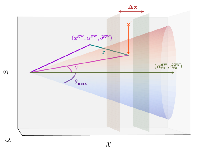
Figure 1: An illustration of the geometry in the three-dimensional Cartesian coordinate system $(\mathcal{XYZ})$ in order to compute the modeled galaxy overdensity $\delta_{g}^{\rm mod}$ following Eq. (9). The geometry corresponding to the computation of the modeled galaxy overdensity is illustrated in Fig. 1. The horizontal arrow denotes the line-of-sight from the observer towards the maximum posterior probability position of the GW event ($\alpha^{\rm gw}_{\rm m},\delta^{\rm gw}_{\rm m}$), the conical volume has an angular radius of $\theta_{\rm max}$ around this position, and the two vertical planes indicate the redshift range of width $\Delta z$, centered at $z$ within which we compute this modeled galaxy overdensity.

In the standard model of cosmology (also known as the $\Lambda\mbox{CDM}$ model), the matter distribution in the Universe forms a cosmic web of large-scale structure with clustering properties determined by the value of cosmological parameters. Dark matter halos form at the peaks of the matter density distribution. The clustering properties of these halos on large scales reflect the clustering properties of the matter distribution, modified with a multiplicative factor $b^{2}$, where $b$ is the linear bias that corresponds to the ratio of the halo overdensity ($\delta_{\rm h}$) to the matter overdensity ($\delta_{\rm m}$),

$$\delta_{\rm h}({\bf x},M)\equiv\frac{n_{\rm h}({\bf x},M)}{\bar{n}_{\rm h}}-1 =b_{\rm h}(M)\delta_{\rm m}({\bf x})\,.$$ (1)

Here, $n_{\rm h}({\bf x},M)$ denotes the number of halos at a given position ${\bf x}$ with halo mass $M$ and $\bar{n}_{\rm h}$ is the average number of halos Cooray and Sheth (2002). The bias of the dark matter halos increases with increasing halo mass (Kaiser, 1984; Tinker et al., 2010). More luminous galaxies are expected to form within more massive dark matter halos Cacciato et al. (2009); Zehavi et al. (2011); More et al. (2011); More (2011); Behroozi et al. (2019), and on large scales, they inherit the bias of the dark matter halos they inhabit, such that

$$b_{\rm g}=\int dMP_{h}(M)b_{h}(M)$$ (2)

where $P_{h}(M)$ specifies the distribution of halo masses to which the galaxies belong Sheth and Tormen (1999); Tinker et al. (2010); Lazeyras et al. (2017) (for a detailed review on the halo and galaxy bias, one may refer to Desjacques et al. (2018)).

In this section, we describe the methodology to utilize the cross-correlation between individual GW events and galaxy catalogs to constrain the Hubble constant. The spatial clustering between galaxies and GW events, separated by the comoving distance ${\bf r}$, can be characterized by the $3$D cross-correlation function, $\xi_{\rm gw,g}({\bf r})$, given by

$$\xi_{\rm gw,g}({\bf r})\equiv\langle\delta_{\rm gw}({\bf x})\delta_{\rm g}({\bf x}+{\bf r})\rangle\,,$$ (3)

where ${\bf x}$ represents the location of GW sources; $\delta_{\rm gw}$ and $\delta_{\rm g}$ denote the overdensity of the GW source distribution and the galaxy distribution, respectively. As the Universe is assumed to be isotropic, the cross-correlation function depends on the scalar distance $r=\lvert{\bf r}\rvert$. Since GW events and galaxies are tracers of the same underlying matter distribution, both GW overdensity and galaxy overdensity are related to the matter overdensity $\delta_{m}$ on large scales as,

$$\delta_{\rm g}=b_{\rm g}\delta_{m}$$ (4a)

$$\delta_{\rm gw}=b_{\rm gw}\delta_{m}$$ (4b)

Here, the proportionality constants $b_{\rm g}$ and $b_{\rm gw}$ are the linear biases of the population of galaxies and GW sources with respect to the matter distribution, respectively. A bias of unity would imply that the observed population follows the underlying matter distribution. In general, the bias parameters depend on different properties of the sources. The dependence of galaxy bias on redshift can be estimated from the measurement of auto-correlation functions of galaxies in a given redshift slice with themselves. The redshift-dependent GW bias needs to be assumed a parametric form and be marginalized over those parameters (see Ref. Mukherjee et al. (2021)).

The cross-correlation function $\xi_{\rm gw,g}$, defined in Eq. 3 can be written as,

$$\xi_{\rm gw,g}=b_{\rm gw}b_{\rm g}\xi_{\rm m}\,.$$ (5)

Here, $\xi_{\rm m}$ is the non-linear matter power spectrum Takahashi et al. (2012), which we compute under the assumption of the standard $\Lambda\mbox{CDM}$ model of cosmology. In the flat $\Lambda\mbox{CDM}$ Universe, the luminosity distance $d_{L}$ is related to the redshift $z$ as follows:

$$d_{L} =\frac{c(1+z)}{H_{0}}\int_{0}^{z}\frac{dz^{\prime}}{H(z^{\prime})}$$

$$=d_{c}(1+z)$$ (6)

Here, $d_{c}$ denotes the comoving distance, and $H(z)$ is the Hubble parameter, expressed in terms of the Hubble constant $H_{0}$ and matter density parameter $\Omega_{m}$ as:

$$H(z)=H_{0}E(z)=H_{0}\sqrt{\Omega_{m}(1+z)^{3}+(1-\Omega_{m})}\ .$$ (7)

Since the correlation function $\xi_{\rm gw,g}(r)$ quantifies the excess probability over a random Poisson distribution of finding a galaxy in a volume element $dV$, which is separated by a comoving distance ${\bf r}$ from a GW event located at position ${\bf x}$, we have

$$n_{\rm g}({\bf x}+{\bf r})dV=\bar{n}_{V}\left[1+\xi_{\rm gw,g}(r)\right]dV\,,$$ (8)

where $\bar{n}_{V}$ is the average number density of galaxies in comoving volume. So, the galaxy overdensity can be calculated by integrating Eq. (8) over some finite volume if we have the theoretical prediction of the non-linear matter power spectrum $\xi_{\rm m}$.

Consider a GW event located at its true position denoted by redshift $z^{\rm gw}$, right ascension $\alpha^{\rm gw}$ and declination $\delta^{\rm gw}$. The modeled galaxy overdensity, $\delta_{g}^{\rm mod}$, in an angle $\theta_{\rm max}$ around the maximum a posteriori probability (MAP) location ($\alpha^{\rm gw}_{\rm m},\delta^{\rm gw}_{\rm m}$) and within a redshift bin centered around $z$, can be computed by carrying out the following volume integral (see Fig. 1 for the geometry),

$$\delta_{g}^{\rm mod}\left(z\mid z^{\rm gw}\left(d_{L}^{\rm gw},H_{0}\right),\alpha^{\rm gw},\delta^{\rm gw}\right)=\frac{\int_{0}^{\theta_{\rm{max}}}\int_{z-\Delta z/2}^{z+\Delta z/2}\bar{n}_{V}(z^{\prime})\xi_{\rm gw,g}(|{\bf r}|)2\pi\sin\theta d_{c}^{\prime~{}2}J\left(\frac{d_{c}^{\prime}}{z^{\prime}}\right)d\theta dz^{\prime}}{\int_{0}^{\theta_{\rm{max}}}\int_{z-\Delta z/2}^{z+\Delta z/2}\bar{n}_{V}(z^{\prime})2\pi\sin\theta d_{c}^{\prime~{}2}J\left(\frac{d_{c}^{\prime}}{z^{\prime}}\right)d\theta dz^{\prime}}\ .$$ (9)

The true GW event redshift can be inferred from the true luminosity distance by inverting Eq. (II). The quantity $d_{c}^{\prime}$ in the above equation denotes the comoving distance corresponding to a redshift $z^{\prime}$ within the redshift bin enclosed by the vertical planes and $J\left(\frac{d_{c}^{\prime}}{z^{\prime}}\right)$ corresponds to the Jacobian of the coordinate transformation from comoving distance to redshift, which can be written as (see, Eq. (II)),

$$J\left(\frac{d_{c}}{z}\right)=\frac{\partial d_{c}}{\partial z}=\frac{c}{H(z)}\,.$$ (10)

The modeled galaxy overdensity thus depends on the choice of $H_{0}$.

The observed galaxy overdensity within the redshift bin, centered around $z$, can be measured within the angular distance $\theta_{\rm max}$ around the line-of-sight towards the MAP position ($\alpha^{\rm gw}_{\rm m},\delta^{\rm gw}_{\rm m}$), as

$$\delta_{g}^{\rm obs}(z)=\frac{n(z\mid\delta^{\rm gw}_{\rm m},\alpha^{\rm gw}_{\rm m})}{\bar{n}(z)}-1\,,$$ (11)

where $n(z\mid\delta^{\rm gw}_{\rm m},\alpha^{\rm gw}_{\rm m})$ denotes the number of galaxies within the redshift bin. For a galaxy survey with uniform depth, the average number of galaxies $\bar{n}(z)$ expected within the redshift bin can be calculated by averaging the observed number of galaxies within the same angular radius $\theta_{\rm max}$ around random lines-of-sight.

The observed overdensity $\delta_{g}^{\rm obs}$ can be calculated in several different redshift bins of galaxies. We call this the galaxy data vector $\bm{d}_{g}^{\rm obs}$. This galaxy data vector can be compared with the model vector of $\delta_{g}^{\rm mod}$ for the same redshift bins of galaxies, denoted by $\bm{d}_{g}^{\rm mod}$ to construct a galaxy overdensity likelihood. Note that the model vector is conditioned on the true location (both on the sky and in redshift) of a particular GW event. The comparison of the two should provide a constraint on the Hubble constant, $H_{0}$.

The true position on which the modeled galaxy overdensity is conditioned has its own uncertainty as the sky localization of the GW event is not precisely known but known as a posterior distribution over $\bm{d}_{\rm gw}=\{d_{L}^{\rm gw},\alpha^{\rm gw},\delta^{\rm gw}\}$ inferred from the gravitational wave strain data $\bm{d}_{\rm strain}$. The posterior for the Hubble constant, in that case, is given by,

$$p(H_{0}\mid\bm{d}_{\rm strain},\bm{d}_{g}^{\rm obs}) =\int p(H_{0},\bm{d}_{\rm gw}\mid\bm{d}_{\rm strain},\bm{d}_{g}^{\rm obs})d\bm{d}_{\rm gw}$$

$$\propto\int{\cal L}(\bm{d}_{\rm strain},\bm{d}_{\rm g}^{\rm obs}|H_{0},\bm{d}_{\rm gw})P(H_{0},\bm{d}_{\rm gw})d\bm{d}_{\rm gw}$$

$$\propto\int{\cal L}(\bm{d}_{\rm g}^{\rm obs}|H_{0},\bm{d}_{\rm gw}){\cal L}(\bm{d}_{\rm strain}|H_{0},\bm{d}_{\rm gw})P(H_{0},\bm{d}_{\rm gw})d\bm{d}_{\rm gw}\,,$$ (12)

where we have applied Bayes’ theorem and assumed independence of the galaxy overdensity and the strain data from gravitational wave events. The integration in the last equation is performed over the localization uncertainty of the GW event. The first likelihood in Eq. (II) corresponds to the galaxy overdensity likelihood, and we assume it to be a Gaussian such that,

$$\mathcal{L}(\bm{d}_{g}^{\rm obs}\mid H_{0},\bm{d}_{\rm gw})\propto\exp\left[-\frac{1}{2}\left(\bm{d}_{g}^{\rm obs}-\bm{d}_{g}^{\rm mod}\right)^{\rm T}\bm{C}^{-1}\left(\bm{d}_{g}^{\rm obs}-\bm{d}_{g}^{\rm mod}\right)\right]$$ (13)

Here, $\bm{C}$ denotes the covariance of the overdensity field, and we assume it to be diagonal with individual elements $\sigma^{2}_{\delta}$ corresponding to the variance in the observed galaxy overdensity in a given redshift bin within the angle $\theta_{\rm max}$. The procedure for calculating $\sigma_{\delta}$ using random lines-of-sight is described in Sec. III.

The second likelihood term in Eq. (II) corresponds to the strain data. Often, the posterior distributions of $P(\bm{d}_{\rm gw})$ are computed assuming certain priors. Therefore, the likelihood can be obtained by taking the ratio of the posteriors for source parameters in $\bm{d}_{\rm gw}$ and the priors that are used to infer these parameters. This allows us to separately impose our own priors on the quantities $p(H_{0},\bm{d}_{\rm gw})$ in Eq. (II).

Since GW events are independent, the final joint posterior of the Hubble constant can be obtained by combining the independent likelihoods of all the detected sources,

$$P(H_{0}\mid\{\bm{d}_{\rm strain}\},\{\bm{d}_{g}^{\rm obs}\}) \propto P(H_{0})\prod_{i}{\cal L}(\bm{d}_{{\rm strain}_{i}},\bm{d}_{g_{i}}^{\rm obs}|H_{0})$$

$$\propto P(H_{0})\prod_{i}\int{\cal L}(\bm{d}_{{\rm strain}_{i}},\bm{d}_{g_{i}}^{\rm obs}|H_{0},\bm{d}_{\rm gw})P(\bm{d}_{\rm gw})d\bm{d}_{\rm gw}$$ (14)

where the index $i$ denotes individual GW events and $\bm{d}_{g_{i}}^{\rm obs}$ is the galaxy overdensity data vector corresponding to the $i^{\rm th}$ GW event.

When constructing the posterior in Eq. (II), we take the flat $\Lambda\mbox{CDM}$ cosmology to be the true cosmological model, with $H_{0}$ as a free parameter and the matter density $\Omega_{m}$ kept fixed at $0.307$. In the flat $\Lambda\mbox{CDM}$ Universe, the relation between luminosity distance $d_{L}$ and the redshift $z$ in Eq. (II) is used to convert the measured luminosity distance of each GW event to its redshift for a given $H_{0}$ whenever required while performing the integral over $\bm{d}_{\rm gw}$ in Eq. (II).

III Simulation

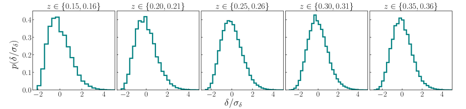
Figure 2: Probability distribution of observed overdensity divided by the corresponding fluctuation in different redshift bins, mentioned at the top of each panel, considering $\theta_{\rm max}=0.03$ radian.

We test the framework discussed in Sec. II with a mock galaxy and GW catalog in order to assess how well the expansion rate can be recovered given realistic localization errors in the positions of GW events. We consider dark matter halos from the Big MultiDark Planck (BigMDPL) cosmological N-body simulation Klypin et al. (2016) from the CosmoSim database  to construct the galaxy catalog. The BigMDPL simulation follows the evolution of the matter distribution in a flat $\Lambda\mbox{CDM}$ cosmology with the following parameters: Hubble parameter $h=H_{0}/(100\ \mbox{km s}^{-1}\,\mbox{Mpc}^{-1})=0.6777$, the matter density parameter $\Omega_{m}=0.307$, the amplitude of density fluctuations characterized by $\sigma_{8}=0.823$ and the power spectrum slope of initial density fluctuations $n_{s}=0.96$. The simulation is set up as $3840^{3}$ collision-less particles in a cubic box with comoving side length $2.5\ h^{-1}{\rm Gpc}$ with periodic boundary conditions and corresponds to a mass resolution of $2.359\times 10^{10}\ h^{-1}M_{\odot}$.

We only consider well-resolved dark matter halos with masses $\geq M_{\rm th}=10^{12}h^{-1}M_{\odot}$. For simplicity, we assume that all galaxies are central galaxies and thus place each galaxy at the center of these dark matter halos. We place an observer at the center of the box and compute the sky positions of each of these mock galaxies with respect to the center, which is within the sphere of radius $1.25\ h^{-1}{\rm Gpc}$. We utilize the cosmological parameters of the simulation to determine the redshift of each galaxy from the comoving distance from the central observer. We use this mock galaxy catalog for further analysis. For simplicity, we have ignored any redshift space distortion effects.

Once we have the mock galaxy catalog, we randomly subselect galaxies to be the hosts of GW events without any regard to the properties of these halos or, equivalently, the properties of the galaxies in the catalog. The true redshifts and sky positions of the GW events are determined from their respective host galaxies in the cosmological box. We use the same cosmological parameters of the simulation box in order to compute the luminosity distance of GW events. The galaxy catalog we use extends up to a comoving distance of $1.25\ h^{-1}{\rm Gpc}$ given the size of the box before we run into incompleteness issues. This comoving distance corresponds to redshift $z\sim 0.46$, assuming the true cosmology. In this work, however, we consider uniform prior over $H_{0}$ between $20~{}\mbox{km s}^{-1}\,\mbox{Mpc}^{-1}$ and $120~{}\mbox{km s}^{-1}\,\mbox{Mpc}^{-1}$. Consequently, a higher value of $H_{0}$ can lead to an increase in the redshift of a GW event at a given luminosity distance. Thus, the GW event can have redshift up to $z\sim 0.36$ when $H_{0}=120~{}\mbox{km s}^{-1}\,\mbox{Mpc}^{-1}$ and yet be detectable in the box. Therefore, we restrict the injection of GW events within a luminosity distance of $1$ Gpc to avoid any biases creeping in due to the above selection effects.

The distribution of the source-frame masses of the BBHs follows the Power Law+Peak model Talbot and Thrane (2018) between minimum mass $m_{\rm min}=5\ M_{\odot}$ and maximum mass $m_{\rm max}=60\ M_{\odot}$. The injected values of other mass hyperparameters (see Appendix B of Ref. Abbott et al. (2021c) for the descriptions of the hyperparameters) are $\lambda_{\rm peak}=0.06,\alpha=3.5,\delta_{m}=4,\mu_{m}=34,\sigma_{m}=5$, $\beta=1.1$, which are consistent with the previous observations Abbott et al. (2021c, 2023b). However, note that the detected masses are redshifted and are expected to differ from the source-frame mass, $m$, as $m_{z}=m(1+z)$, where $z$ is the redshift of the event. The other BBH parameters (see Table 1 of Ref. Ashton et al. (2019) for the list of parameters) are randomly chosen from the default priors of  bilby (see Table 1 of Ref. Ashton et al. (2019) for the default priors). The simulated BBH signal is added to stationary Gaussian noise, colored with the O4 design sensitivity Abbott et al. (2018) of LIGO and Virgo detectors. We analyze the strain signal between $20$ Hz and $2048$ Hz to infer the source parameters. We consider the same non-precessing waveform model IMRPhenomD Khan et al. (2016) for both the signal injection and recovery. We have used the nested sampler dynesty Speagle (2020) implemented in bilby Ashton et al. (2019) to infer the posterior distribution of all the parameters given the waveform. We consider uniform prior over chirp mass and mass ratio. This choice of priors for mass parameters is convenient for efficient sampling. We employ cosmology independent $d_{L}^{2}$ prior to the luminosity distance of the source. The priors over the rest of the extrinsic parameters are the default priors implemented in bilby (refer to Table $1$ in Ref. Ashton et al. (2019) for the default priors).

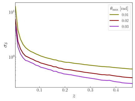
Figure 3: Observed overdensity fluctuation as a function of redshift over $10^{6}$ random line of sights.

The parameters thus inferred are utilized to constrain $H_{0}$ by cross-correlating the localization of these individual events with galaxies in the mock catalog. We are primarily interested in the extrinsic source parameters, such as $d_{L}^{\rm gw}$, $\alpha^{\rm gw}$ and $\delta^{\rm gw}$ in this work. So, we compute the GW likelihood $\mathcal{L}_{\rm gw}$ by marginalizing over the rest of the intrinsic and extrinsic parameters. The galaxy overdensity likelihood $\mathcal{L}_{g}$ is also calculated for different sky coordinates within the localization of the GW events as a function of redshift in order to perform the integration of Eq. (II). The galaxy overdensity likelihood includes the computation of the observed and modeled galaxy overdensity fields as a function of redshift. The modeled galaxy overdensity is calculated from the cross-correlation function $\xi$ (see, Eq. (9)), which depends on the separation (comoving distance in $h^{-1}$ scale) between the GW event and the redshift where the observed galaxy overdensity is also measured. We have used the publicly available code AUM  to compute $\xi$ van den Bosch et al. (2013) from the non-linear matter power spectrum Takahashi et al. (2012) assuming the flat $\Lambda\mbox{CDM}$ cosmology. To study the effect of the cross-correlation length-scale on the $H_{0}$ estimation, we assume $4$ different values of the angular radius $\theta_{\rm max}$ (elaborated in Sec. IV) along the line-of-sight to calculate the observed and modeled galaxy overdensity fields.

In order to compute the likelihood of observing the galaxy overdensity given the modeled overdensity, we quantify the variance of the galaxy overdensity field (denoted as $\sigma^{2}_{\delta}$ in Eq. (II)) around random lines-of-sight at each redshift bin. The variance of the overdensity depends upon the specific value of $\theta_{\rm max}$ over which we average. We use $10^{6}$ random lines-of-sight within the mock galaxy catalog used in this work. The probability distribution of $\delta/\sigma$ for $5$ representative redshift bins of width $\Delta z=0.01$ up to $z=0.36$ are shown in Fig. 2, for $\theta_{\rm max}=0.03$ radian. The corresponding standard deviation of the overdensity field is shown as a function of redshift as solid lines in Fig. 3, where the colors signify different values of $\theta_{\rm max}$. As expected, $\sigma$ decreases with redshift for any $\theta_{\rm max}$ due to the increase in cosmological volume probed within the angular region per redshift interval. Similarly, a higher value of $\theta_{\rm max}$ also results in a smaller standard deviation for the overdensity at any given redshift. Notably, the redshift width of $\Delta z=0.01$ for calculating galaxy overdensity has been carefully selected to ensure a sufficient number of galaxies in each redshift bin. We use this variance in order to evaluate the likelihood of the galaxy overdensity given the modeled overdensity and a true position of the GW event, which, among other parameters, depends upon the Hubble constant. In order to infer the posterior distribution of the Hubble constant given the data, we assume a uniform prior in $H_{0}\in U[20,120]\ \mbox{km s}^{-1}\,\mbox{Mpc}^{-1}$. We finally infer the joint posterior for $H_{0}$ for multiple events as given by Eq. (II).

IV Results

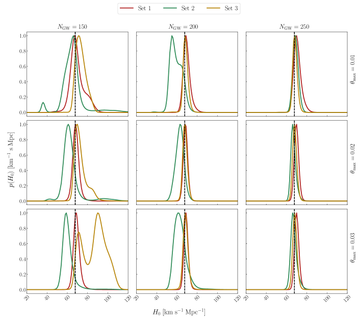
Figure 4: Estimation of Hubble constant from BBH events whose network SNR $\rho_{\rm net}\geq 12$, as detected by LIGO-Virgo detector operating at O4 sensitivity, for different choices of $\theta_{\rm max}$ (in radian). The black vertical dashed line in each of the plots corresponds to the injected value of $H_{0}=67.77\mbox{km s}^{-1}\,\mbox{Mpc}^{-1}$.

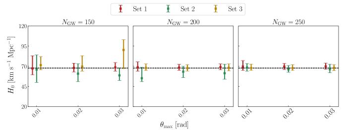
Figure 5: Uncertainty corresponding to $90\%$ highest density interval in estimating $H_{0}$ from different subsets of GW events for various values of $\theta_{\rm max}$ . The dashed horizontal line in each of the plots corresponds to the true value of $H_{0}=67.77\ \mbox{km s}^{-1}\,\mbox{Mpc}^{-1}$. Each plot corresponds to $3$ different sets of a fixed number of GW events, mentioned at the top of the corresponding plot. $H_{0}$ error bar plot of set 2 GW events corresponds to the correct $\theta_{\rm max}$. However, $H_{0}$ error bar plot of set 1 and set 3 GW events are plotted with the offsets of $-0.001$ and $0.001$ radian in $\theta_{\rm max}$. These offsets are used for illustration purposes only.

We apply our method as mentioned in Sec. II to $3$ different mock GW catalogs for $3$ different choices of $\theta_{\rm max}=\left\{0.01,0.02,0.03\right\}$ radian to study the statistical robustness. The GW catalogs are random realizations of the same population, as discussed in Sec. III. Each GW catalog consists of $250$ simulated GW events that are detected with a network SNR $\rho_{\rm net}\geq 12$ in the three LIGO-Virgo detectors, with O4 design sensitivity Abbott et al. (2018). We also study $H_{0}$ posteriors for $2$ subsets of $150$ and $200$ GW events from those $3$ sets of $250$ detected GW events. The threshold on network SNR in this work is chosen based on the earlier LVK cosmology papers Abbott et al. (2021b, 2023a). Sources with low network SNR would not contribute significantly to the improvement in the inference of the Hubble constant due to the poor sky localization and larger uncertainty in distance measurement. Fig. 4 shows the $H_{0}$ posteriors for $3$ different sets of GW events with varying numbers of detected events. Each row of Fig. 4 corresponds to a particular value of $\theta_{\rm max}$, mentioned in the right of the figure for different numbers of GW events. The columns of Fig. 4 correspond to $H_{0}$ posteriors for a fixed number of GW events, mentioned at the top of that panel, with varying $\theta_{\rm max}$. The black vertical dashed lines correspond to the injected value of $H_{0}=67.77~{}\mbox{km s}^{-1}\,\mbox{Mpc}^{-1}$ in Fig. 4.

We also summarize the uncertainty corresponding to $90\%$ highest density interval in constraining $H_{0}$ in Fig. 5 for different number of detected GW events. The different panels correspond to varying numbers of detected events $N_{\rm GW}$. In each panel, the error bar of $H_{0}$ uncertainty for $3$ different sets are depicted with $3$ different colors. Set $1$ and $3$ have offsets of $-0.001$ and $0.001$ radian, respectively, corresponding to the true $\theta_{\rm max}$ for clarity in the representation. In Fig. 5, the black horizontal dashed lines represent the injected value of $H_{0}=67.77~{}\mbox{km s}^{-1}\,\mbox{Mpc}^{-1}$.

As expected, the posterior of $H_{0}$ starts to converge to the true value of $H_{0}=67.77~{}\mbox{km s}^{-1}\,\mbox{Mpc}^{-1}$ with increasing number of GW events. However, for the smaller number of GW events $\sim 150$, the $H_{0}$ posteriors can show a wide variation. We speculate that the non-Gaussian nature of galaxy overdensity fluctuation $\sigma_{\delta}$ (see Fig 2) and not accounting for the covariance between different redshift bins is likely the reason for this wide variation. Though this is not an issue for unbiased estimation of $H_{0}$ with larger GW events, it is an aspect that needs to be carefully explored in the future. We have studied $H_{0}$ posteriors for larger $\theta_{\rm max}>0.03$ radian and found the posteriors degrade even when the number of GW events is significant, i.e., $\gtrsim 150$. This is likely related to the fact that large values of $\theta_{\rm max}$ would decrease the amplitude of the correlation signal, reducing the total signal-to-noise ratio.

On the other hand, we have observed it becomes difficult to capture the correlation signal for smaller values of $\theta_{\rm max}\lesssim 0.005$ radian due to the significant fluctuation in measuring the clustering for a smaller number of galaxies, especially at low redshift. So, it is crucial to explore the optimal value of $\theta_{\rm max}$ to perform this method for unbiased estimation of the Hubble constant. From Fig. 5, we observe that $\theta_{\rm max}=0.02$ radian may be the optimal choice in our study. However, the optimal value of $\theta_{\rm max}$ may vary for different GW events. In this work, we keep the values of $\theta_{\rm max}$ fixed for all GW events for simplicity. We leave the exercise of finding the optimal $\theta_{\rm max}$ given the localization area on the sky to investigations in the future.

$N_{\rm GW}$	$\theta_{\rm max}$ (radian)	$H_{0}($$\mbox{km s}^{-1}\,\mbox{Mpc}^{-1}$ $)$
		Set $1$	Set $2$	Set $3$
$150$	$0.01$	$67.30^{+15.69}_{-7.84}$	$65.97^{+18.19}_{-15.97}$	$71.41^{+10.59}_{-5.77}$
	$0.02$	$68.10^{+5.74}_{-5.10}$	$60.90^{+12.26}_{-9.90}$	$69.57^{+13.50}_{-5.57}$
	$0.03$	$68.65^{+5.91}_{-4.64}$	$58.73^{+9.27}_{-6.29}$	$90.28^{12.72}_{-23.01}$
$200$	$0.01$	$68.76^{+6.71}_{-4.76}$	$55.24^{+13.59}_{-4.24}$	$68.02^{+4.97}_{-3.19}$
	$0.02$	$68.37^{+4.09}_{-3.37}$	$63.34^{+6.58}_{-7.34}$	$67.64^{+4.35}_{-3.51}$
	$0.03$	$68.85^{+4.14}_{-3.23}$	$61.42^{+11.07}_{-7.42}$	$68.22^{+4.78}_{-3.90}$
$250$	$0.01$	$69.66^{+7.41}_{-4.67}$	$68.53^{+4.92}_{-4.53}$	$67.82^{+4.84}_{-2.82}$
	$0.02$	$69.68^{+3.83}_{-3.68}$	$66.07^{+4.93}_{-3.48}$	$66.07^{+4.92}_{-3.48}$
	$0.03$	$69.84^{+4.15}_{-3.54}$	$66.30^{+6.18}_{-4.30}$	$68.00^{+4.00}_{-3.34}$

Table 1: Summary of uncertainty (maximum a posteriori probability with $90\%$ highest density interval) of inferred values of the Hubble constant from different sets of GW events with varying $\theta_{\rm max}$.

We report the $90\%$ highest density interval of the inferred values of $H_{0}$ corresponding to the three different sets in Table 1 for $3$ different choices of $\theta_{\rm max}=\left\{0.01,0.02,0.03\right\}$ radian. The corresponding $H_{0}$ posteriors are also shown in Fig. 5. We observe that we can constrain $H_{0}$ with a precision of $\lesssim 15\%$ ($90\%$ highest density interval) by combining the individual $H_{0}$ posterior from $250$ GW events. It is important to note that we consider GW events within $1$ Gpc as the mock galaxy catalog used in this work is volume limited, extending up to redshift $z\sim 0.46$, already detailed in Sec. III. The sky localizations of these simulated GW events are better than those from larger distances, which are observed by the current generation detectors. So, the broad sky localizations of GW events from significantly large distances may affect $H_{0}$ estimation and result in broadening the $H_{0}$ posterior.

V Discussion

Observations of GWs from coalescing binaries provide the direct measurement of the luminosity distance unaffected by systematics in various external astrophysical calibrations that rely on the cosmic distance ladder. However, GW estimates can be biased due to systematics inherent to its measurements, such as GW detector calibration Sun et al. (2021); Bhattacharjee et al. (2021). Assuming that the instrument can be calibrated sufficiently accurately Sun et al. (2021); Bhattacharjee et al. (2021), GW sources can be used to estimate the Hubble constant and other cosmological parameters. However, redshift information is not available from GW observations. Additionally, most of the detected GW events are BBH mergers and are not accompanied by EM counterparts. In this paper, we successfully demonstrated the inference of the Hubble constant from individual GW events by cross-correlating with the galaxy catalog. This method is useful even if the mergers do not have any EM observations and can supplement the inference of the Hubble constant from BNS mergers with detected EM counterparts.

Our method consists of measuring the galaxy overdensity as a function of redshift at the maximum a posteriori probability in the sky localization of individual gravitational wave events. We compare the data vector of observed galaxy overdensity $\bm{d}_{g}^{\rm obs}$ with that of the modeled galaxy overdensity $\bm{d}_{g}^{\rm mod}$ which depends on the value of $H_{0}$, to define a likelihood and infer the posterior distribution of $H_{0}$ in a Bayesian analysis. As examples, we considered $3$ different mock GW catalog to infer $H_{0}$ using the method described in Sec. II and were able to constrain the Hubble constant with an accuracy of $\lesssim 15\%$ ($90\%$ highest density interval). The efficacy of the method is tested for the second-generation detector network comprising of the Advanced LIGO Aasi et al. (2015) and Advanced Virgo Acernese et al. (2015) detectors. With the improved sensitivity in the third-generation detectors like Cosmic Explorer Evans et al. (2021) and Einstein Telescope Maggiore et al. (2020), GW sources will be detected with much higher detection rate and, therefore, precise estimation of luminosity distance and sky localization. We expect this method to constrain $H_{0}$ with higher precision with such detectors.

In our current analysis, we have only considered $H_{0}$ as a free parameter to be constrained from the GW and galaxy overdensity observations. However, it is straightforward to extend our analysis to constrain other cosmological parameters, such as the matter density at the current epoch and dark energy equation-of-state. We do not consider them here to avoid the extra computational costs involved in estimating cosmological parameter(s). With the second-generation GW detectors, cosmological parameters except for $H_{0}$ are expected to be weakly constrained Abbott et al. (2023a).

Our results show that the cross-correlation method can be utilized to infer $H_{0}$ from individuals from GW events as a proof-of-concept. We have made several simplifying assumptions in this work. The mock galaxy catalog used here is assumed to be volume-limited instead of being flux-limited. We have also considered the idealistic scenario where the GW events are the unbiased tracers of underlying matter distribution. In reality, the GW events and the galaxies trace the large-scale structure with a redshift-dependent bias Vijaykumar et al. (2023); Libanore et al. (2021). This redshift-dependent bias could arise from the evolving way in which the gravitational wave events populate dark matter halos or due to selection effects. These effects need to be parameterized and marginalized to constrain the cosmological parameters from real data. We also have not accounted for any impact that weak gravitational lensing will have on the luminosity distance estimates due to the intervening large-scale structure Oguri (2016). Weak lensing induces a non-trivial spatial correlation on the sky at redshifts lower than that of the GW events. It should be incorporated into our methodology while working with real data, especially for high redshift events. This is currently beyond the scope of this work and will be investigated further in future studies.

References

- Abbott et al. (2017a) B. P. Abbott et al. (LIGO Scientific, Virgo), “GW170817: Observation of Gravitational Waves from a Binary Neutron Star Inspiral,” Phys. Rev. Lett. 119, 161101 (2017a), arXiv:1710.05832 [gr-qc] .
- Abbott et al. (2017b) B. P. Abbott et al. (LIGO Scientific, Virgo, Fermi GBM, INTEGRAL, IceCube, AstroSat Cadmium Zinc Telluride Imager Team, IPN, Insight-Hxmt, ANTARES, Swift, AGILE Team, 1M2H Team, Dark Energy Camera GW-EM, DES, DLT40, GRAWITA, Fermi-LAT, ATCA, ASKAP, Las Cumbres Observatory Group, OzGrav, DWF (Deeper Wider Faster Program), AST3, CAASTRO, VINROUGE, MASTER, J-GEM, GROWTH, JAGWAR, CaltechNRAO, TTU-NRAO, NuSTAR, Pan-STARRS, MAXI Team, TZAC Consortium, KU, Nordic Optical Telescope, ePESSTO, GROND, Texas Tech University, SALT Group, TOROS, BOOTES, MWA, CALET, IKI-GW Follow-up, H.E.S.S., LOFAR, LWA, HAWC, Pierre Auger, ALMA, Euro VLBI Team, Pi of Sky, Chandra Team at McGill University, DFN, ATLAS Telescopes, High Time Resolution Universe Survey, RIMAS, RATIR, SKA South Africa/MeerKAT), “Multi-messenger Observations of a Binary Neutron Star Merger,” Astrophys. J. Lett. 848, L12 (2017b), arXiv:1710.05833 [astro-ph.HE] .
- Abbott et al. (2017c) B. P. Abbott et al. (LIGO Scientific, Virgo, 1M2H, Dark Energy Camera GW-E, DES, DLT40, Las Cumbres Observatory, VINROUGE, MASTER), “A gravitational-wave standard siren measurement of the Hubble constant,” Nature 551, 85–88 (2017c), arXiv:1710.05835 [astro-ph.CO] .
- Aasi et al. (2015) J. Aasi et al. (LIGO Scientific), “Advanced LIGO,” Class. Quant. Grav. 32, 074001 (2015), arXiv:1411.4547 [gr-qc] .
- Acernese et al. (2015) F. Acernese et al. (VIRGO), “Advanced Virgo: a second-generation interferometric gravitational wave detector,” Class. Quant. Grav. 32, 024001 (2015), arXiv:1408.3978 [gr-qc] .
- Akutsu et al. (2019) T. Akutsu et al. (KAGRA), “KAGRA: 2.5 Generation Interferometric Gravitational Wave Detector,” Nature Astron. 3, 35–40 (2019), arXiv:1811.08079 [gr-qc] .
- Abbott et al. (2021a) R. Abbott et al. (LIGO Scientific, VIRGO, KAGRA), “GWTC-3: Compact Binary Coalescences Observed by LIGO and Virgo During the Second Part of the Third Observing Run,” (2021a), arXiv:2111.03606 [gr-qc] .
- Schutz (1986) B. F. Schutz, “Determining the Hubble constant from gravitational wave observations,” Nature (London) 323, 310–311 (1986).
- Del Pozzo (2012) Walter Del Pozzo, “Inference of the cosmological parameters from gravitational waves: application to second generation interferometers,” Phys. Rev. D 86, 043011 (2012), arXiv:1108.1317 [astro-ph.CO] .
- Chen et al. (2018) Hsin-Yu Chen, Maya Fishbach, and Daniel E. Holz, “A two per cent Hubble constant measurement from standard sirens within five years,” Nature 562, 545–547 (2018), arXiv:1712.06531 [astro-ph.CO] .
- Soares-Santos et al. (2019) M. Soares-Santos et al. (DES, LIGO Scientific, Virgo), “First Measurement of the Hubble Constant from a Dark Standard Siren using the Dark Energy Survey Galaxies and the LIGO/Virgo Binary–Black-hole Merger GW170814,” Astrophys. J. Lett. 876, L7 (2019), arXiv:1901.01540 [astro-ph.CO] .
- Gray et al. (2020) Rachel Gray et al., “Cosmological inference using gravitational wave standard sirens: A mock data analysis,” Phys. Rev. D 101, 122001 (2020), arXiv:1908.06050 [gr-qc] .
- Abbott et al. (2021b) B. P. Abbott et al. (LIGO Scientific, Virgo, VIRGO), “A Gravitational-wave Measurement of the Hubble Constant Following the Second Observing Run of Advanced LIGO and Virgo,” Astrophys. J. 909, 218 (2021b), arXiv:1908.06060 [astro-ph.CO] .
- Abbott et al. (2020) R. Abbott et al. (LIGO Scientific, Virgo), “GW190814: Gravitational Waves from the Coalescence of a 23 Solar Mass Black Hole with a 2.6 Solar Mass Compact Object,” Astrophys. J. Lett. 896, L44 (2020), arXiv:2006.12611 [astro-ph.HE] .
- Gray et al. (2022) Rachel Gray, Chris Messenger, and John Veitch, “A pixelated approach to galaxy catalogue incompleteness: improving the dark siren measurement of the Hubble constant,” Mon. Not. Roy. Astron. Soc. 512, 1127–1140 (2022), arXiv:2111.04629 [astro-ph.CO] .
- Farr et al. (2019) Will M. Farr, Maya Fishbach, Jiani Ye, and Daniel Holz, “A Future Percent-Level Measurement of the Hubble Expansion at Redshift 0.8 With Advanced LIGO,” Astrophys. J. Lett. 883, L42 (2019), arXiv:1908.09084 [astro-ph.CO] .
- You et al. (2021) Zhi-Qiang You, Xing-Jiang Zhu, Gregory Ashton, Eric Thrane, and Zong-Hong Zhu, “Standard-siren cosmology using gravitational waves from binary black holes,” Astrophys. J. 908, 215 (2021), arXiv:2004.00036 [astro-ph.CO] .
- Mastrogiovanni et al. (2021) S. Mastrogiovanni, K. Leyde, C. Karathanasis, E. Chassande-Mottin, D. A. Steer, J. Gair, A. Ghosh, R. Gray, S. Mukherjee, and S. Rinaldi, “On the importance of source population models for gravitational-wave cosmology,” Phys. Rev. D 104, 062009 (2021), arXiv:2103.14663 [gr-qc] .
- Abbott et al. (2019) B. P. Abbott et al. (LIGO Scientific, Virgo), “Properties of the binary neutron star merger GW170817,” Phys. Rev. X 9, 011001 (2019), arXiv:1805.11579 [gr-qc] .
- Abbott et al. (2023a) R. Abbott et al. (LIGO Scientific, Virgo,, KAGRA, VIRGO), “Constraints on the Cosmic Expansion History from GWTC–3,” Astrophys. J. 949, 76 (2023a), arXiv:2111.03604 [astro-ph.CO] .
- Mastrogiovanni et al. (2023) Simone Mastrogiovanni, Danny Laghi, Rachel Gray, Giada Caneva Santoro, Archisman Ghosh, Christos Karathanasis, Konstantin Leyde, Daniele A. Steer, Stephane Perries, and Gregoire Pierra, “Joint population and cosmological properties inference with gravitational waves standard sirens and galaxy surveys,” Phys. Rev. D 108, 042002 (2023), arXiv:2305.10488 [astro-ph.CO] .
- Gray et al. (2023) Rachel Gray et al., “Joint cosmological and gravitational-wave population inference using dark sirens and galaxy catalogues,” JCAP 12, 023 (2023), arXiv:2308.02281 [astro-ph.CO] .
- Messenger and Read (2012) C. Messenger and J. Read, “Measuring a cosmological distance-redshift relationship using only gravitational wave observations of binary neutron star coalescences,” Phys. Rev. Lett. 108, 091101 (2012), arXiv:1107.5725 [gr-qc] .
- Chatterjee et al. (2021) Deep Chatterjee, Abhishek Hegade K R, Gilbert Holder, Daniel E. Holz, Scott Perkins, Kent Yagi, and Nicolás Yunes, “Cosmology with Love: Measuring the Hubble constant using neutron star universal relations,” Phys. Rev. D 104, 083528 (2021), arXiv:2106.06589 [gr-qc] .
- Jin et al. (2023) Shang-Jie Jin, Tian-Nuo Li, Jing-Fei Zhang, and Xin Zhang, “Prospects for measuring the Hubble constant and dark energy using gravitational-wave dark sirens with neutron star tidal deformation,” JCAP 08, 070 (2023), arXiv:2202.11882 [gr-qc] .
- Ghosh et al. (2022) Tathagata Ghosh, Bhaskar Biswas, and Sukanta Bose, “Simultaneous inference of neutron star equation of state and the Hubble constant with a population of merging neutron stars,” Phys. Rev. D 106, 123529 (2022), arXiv:2203.11756 [astro-ph.CO] .
- Shiralilou et al. (2022) Banafsheh Shiralilou, Geert Raaiijmakers, Bastien Duboeuf, Samaya Nissanke, Francois Foucart, Tanja Hinderer, and Andrew Williamson, “Measuring Hubble Constant with Dark Neutron Star-Black Hole Mergers,” (2022), arXiv:2207.11792 [astro-ph.CO] .
- Dhani et al. (2022) Arnab Dhani, Ssohrab Borhanian, Anuradha Gupta, and Bangalore Sathyaprakash, “Cosmography with bright and Love sirens,” (2022), arXiv:2212.13183 [gr-qc] .
- (29) Tathagata Ghosh et al., (in preparation) .
- MacLeod and Hogan (2008) Chelsea L. MacLeod and Craig J. Hogan, “Precision of Hubble constant derived using black hole binary absolute distances and statistical redshift information,” Phys. Rev. D 77, 043512 (2008), arXiv:0712.0618 [astro-ph] .
- Oguri (2016) Masamune Oguri, “Measuring the distance-redshift relation with the cross-correlation of gravitational wave standard sirens and galaxies,” Phys. Rev. D 93, 083511 (2016), arXiv:1603.02356 [astro-ph.CO] .
- Bera et al. (2020) Sayantani Bera, Divya Rana, Surhud More, and Sukanta Bose, “Incompleteness Matters Not: Inference of from Binary Black Hole–Galaxy Cross-correlations,” Astrophys. J. 902, 79 (2020), arXiv:2007.04271 [astro-ph.CO] .
- Mukherjee et al. (2020) Suvodip Mukherjee, Benjamin D. Wandelt, and Joseph Silk, “Probing the theory of gravity with gravitational lensing of gravitational waves and galaxy surveys,” Mon. Not. Roy. Astron. Soc. 494, 1956–1970 (2020), arXiv:1908.08951 [astro-ph.CO] .
- Mukherjee et al. (2021) Suvodip Mukherjee, Benjamin D. Wandelt, Samaya M. Nissanke, and Alessandra Silvestri, “Accurate precision Cosmology with redshift unknown gravitational wave sources,” Phys. Rev. D 103, 043520 (2021), arXiv:2007.02943 [astro-ph.CO] .
- Diaz and Mukherjee (2022) Cristina Cigarran Diaz and Suvodip Mukherjee, “Mapping the cosmic expansion history from LIGO-Virgo-KAGRA in synergy with DESI and SPHEREx,” Mon. Not. Roy. Astron. Soc. 511, 2782–2795 (2022), arXiv:2107.12787 [astro-ph.CO] .
- Mukherjee et al. (2022) Suvodip Mukherjee, Alex Krolewski, Benjamin D. Wandelt, and Joseph Silk, “Cross-correlating dark sirens and galaxies: measurement of from GWTC-3 of LIGO-Virgo-KAGRA,” (2022), arXiv:2203.03643 [astro-ph.CO] .
- Cooray and Sheth (2002) Asantha Cooray and Ravi K. Sheth, “Halo Models of Large Scale Structure,” Phys. Rept. 372, 1–129 (2002), arXiv:astro-ph/0206508 .
- Kaiser (1984) Nick Kaiser, “On the Spatial correlations of Abell clusters,” Astrophys. J. Lett. 284, L9–L12 (1984).
- Tinker et al. (2010) Jeremy L. Tinker, Brant E. Robertson, Andrey V. Kravtsov, Anatoly Klypin, Michael S. Warren, Gustavo Yepes, and Stefan Gottlöber, “The large-scale bias of dark matter halos: Numerical calibration and model tests,” The Astrophysical Journal 724, 878 (2010).
- Cacciato et al. (2009) Marcello Cacciato, Frank C. van den Bosch, Surhud More, Ran Li, H. J. Mo, and Xiaohu Yang, “Galaxy Clustering & Galaxy-Galaxy Lensing: A Promising Union to Constrain Cosmological Parameters,” Mon. Not. Roy. Astron. Soc. 394, 929–946 (2009), arXiv:0807.4932 [astro-ph] .
- Zehavi et al. (2011) Idit Zehavi, Zheng Zheng, David H. Weinberg, Michael R. Blanton, Neta A. Bahcall, Andreas A. Berlind, Jon Brinkmann, Joshua A. Frieman, James E. Gunn, Robert H. Lupton, Robert C. Nichol, Will J. Percival, Donald P. Schneider, Ramin A. Skibba, Michael A. Strauss, Max Tegmark, and Donald G. York, “Galaxy Clustering in the Completed SDSS Redshift Survey: The Dependence on Color and Luminosity,” Astrophys. J. 736, 59 (2011), arXiv:1005.2413 [astro-ph.CO] .
- More et al. (2011) Surhud More, Frank C. van den Bosch, Marcello Cacciato, Ramin Skibba, H. J. Mo, and Xiaohu Yang, “Satellite kinematics - III. Halo masses of central galaxies in SDSS,” Mon. Not. Roy. Astron. Soc. 410, 210–226 (2011), arXiv:1003.3203 [astro-ph.CO] .
- More (2011) Surhud More, “How accurate is our knowledge of galaxy bias?” Astrophys. J. 741, 19 (2011), arXiv:1107.1498 [astro-ph.CO] .
- Behroozi et al. (2019) Peter Behroozi, Risa H. Wechsler, Andrew P. Hearin, and Charlie Conroy, “UNIVERSEMACHINE: The correlation between galaxy growth and dark matter halo assembly from z = 0-10,” Mon. Not. Roy. Astron. Soc. 488, 3143–3194 (2019), arXiv:1806.07893 [astro-ph.GA] .
- Sheth and Tormen (1999) Ravi K. Sheth and Giuseppe Tormen, “Large scale bias and the peak background split,” Mon. Not. Roy. Astron. Soc. 308, 119 (1999), arXiv:astro-ph/9901122 .
- Lazeyras et al. (2017) Titouan Lazeyras, Marcello Musso, and Fabian Schmidt, “Large-scale assembly bias of dark matter halos,” Journal of Cosmology and Astroparticle Physics 2017, 059 (2017).
- Desjacques et al. (2018) Vincent Desjacques, Donghui Jeong, and Fabian Schmidt, “Large-scale galaxy bias,” Physics Reports 733, 1–193 (2018).
- Takahashi et al. (2012) Ryuichi Takahashi, Masanori Sato, Takahiro Nishimichi, Atsushi Taruya, and Masamune Oguri, “Revising the Halofit Model for the Nonlinear Matter Power Spectrum,” Astrophys. J. 761, 152 (2012), arXiv:1208.2701 [astro-ph.CO] .
- Klypin et al. (2016) Anatoly Klypin, Gustavo Yepes, Stefan Gottlober, Francisco Prada, and Steffen Hess, “MultiDark simulations: the story of dark matter halo concentrations and density profiles,” Mon. Not. Roy. Astron. Soc. 457, 4340–4359 (2016), arXiv:1411.4001 [astro-ph.CO] .
- Talbot and Thrane (2018) Colm Talbot and Eric Thrane, “Measuring the binary black hole mass spectrum with an astrophysically motivated parameterization,” Astrophys. J. 856, 173 (2018), arXiv:1801.02699 [astro-ph.HE] .
- Abbott et al. (2021c) R. Abbott et al. (LIGO Scientific, Virgo), “Population Properties of Compact Objects from the Second LIGO-Virgo Gravitational-Wave Transient Catalog,” Astrophys. J. Lett. 913, L7 (2021c), arXiv:2010.14533 [astro-ph.HE] .
- Abbott et al. (2023b) R. Abbott et al. (KAGRA, VIRGO, LIGO Scientific), “Population of Merging Compact Binaries Inferred Using Gravitational Waves through GWTC-3,” Phys. Rev. X 13, 011048 (2023b), arXiv:2111.03634 [astro-ph.HE] .
- Ashton et al. (2019) Gregory Ashton, Moritz Hübner, Paul D. Lasky, Colm Talbot, Kendall Ackley, Sylvia Biscoveanu, Qi Chu, Atul Divakarla, Paul J. Easter, Boris Goncharov, and et al., “Bilby: A user-friendly bayesian inference library for gravitational-wave astronomy,” The Astrophysical Journal Supplement Series 241, 27 (2019).
- Abbott et al. (2018) B. P. Abbott et al. (KAGRA, LIGO Scientific, Virgo, VIRGO), “Prospects for observing and localizing gravitational-wave transients with Advanced LIGO, Advanced Virgo and KAGRA,” Living Rev. Rel. 21, 3 (2018), arXiv:1304.0670 [gr-qc] .
- Khan et al. (2016) Sebastian Khan, Sascha Husa, Mark Hannam, Frank Ohme, Michael Pürrer, Xisco Jiménez Forteza, and Alejandro Bohé, “Frequency-domain gravitational waves from nonprecessing black-hole binaries. II. A phenomenological model for the advanced detector era,” Phys. Rev. D 93, 044007 (2016), arXiv:1508.07253 [gr-qc] .
- Speagle (2020) Joshua S. Speagle, “Dynesty: a dynamic nested sampling package for estimating bayesian posteriors and evidences,” Mon. Not. Roy. Astron. Soc. 493, 3132–3158 (2020), arXiv:1904.02180 [astro-ph.IM] .
- van den Bosch et al. (2013) Frank C. van den Bosch, Surhud More, Marcello Cacciato, Houjun Mo, and Xiaohu Yang, “Cosmological constraints from a combination of galaxy clustering and lensing - I. Theoretical framework,” Mon. Not. Roy. Astron. Soc. 430, 725–746 (2013), arXiv:1206.6890 [astro-ph.CO] .
- Sun et al. (2021) Ling Sun et al., “Characterization of systematic error in Advanced LIGO calibration in the second half of O3,” (2021), arXiv:2107.00129 [astro-ph.IM] .
- Bhattacharjee et al. (2021) D. Bhattacharjee, Y. Lecoeuche, S. Karki, J. Betzwieser, V. Bossilkov, S. Kandhasamy, E. Payne, and R. L. Savage, “Fiducial displacements with improved accuracy for the global network of gravitational wave detectors,” Class. Quant. Grav. 38, 015009 (2021), arXiv:2006.00130 [astro-ph.IM] .
- Evans et al. (2021) Matthew Evans et al., “A Horizon Study for Cosmic Explorer: Science, Observatories, and Community,” (2021), arXiv:2109.09882 [astro-ph.IM] .
- Maggiore et al. (2020) Michele Maggiore et al., “Science Case for the Einstein Telescope,” JCAP 03, 050 (2020), arXiv:1912.02622 [astro-ph.CO] .
- Vijaykumar et al. (2023) Aditya Vijaykumar, M. V. S. Saketh, Sumit Kumar, Parameswaran Ajith, and Tirthankar Roy Choudhury, “Probing the large scale structure using gravitational-wave observations of binary black holes,” Phys. Rev. D 108, 103017 (2023), arXiv:2005.01111 [astro-ph.CO] .
- Libanore et al. (2021) S. Libanore, M. C. Artale, D. Karagiannis, M. Liguori, N. Bartolo, Y. Bouffanais, N. Giacobbo, M. Mapelli, and S. Matarrese, “Gravitational Wave mergers as tracers of Large Scale Structures,” JCAP 02, 035 (2021), arXiv:2007.06905 [astro-ph.CO] .