Effective dynamics of quantum fluctuations in field theory: with applications to cosmology

Abstract

We develop a novel framework for describing quantum fluctuations in field theory, with a focus on cosmological applications. Our method uniquely circumvents the use of operator/Hilbert-space formalism, instead relying on a systematic treatment of classical variables, quantum fluctuations, and an effective Hamiltonian. Our framework not only aligns with standard formalisms in flat and de Sitter spacetimes, which assumes no backreaction, demonstrated through the $\varphi^{3}$-model, but also adeptly handles time-dependent backreaction in more general cases. The uncertainty principle and spatial symmetry emerge as critical tools for selecting initial conditions and understanding effective potentials. We discover that modes inside the Hubble horizon do not necessarily feel an initial Minkowski vacuum, as is commonly assumed. Our findings offer fresh insights into the early universe’s quantum fluctuations and potential explanations to large-scale CMB anomalies.

1 Introduction

The framework of inflation explains elegantly how quantum fluctuations of the early universe can seed a Gaussian primordial power spectrum. This primordial power spectrum would then grow to form the inhomogeneous structures of our universe — the temperature correlations of the cosmic microwave background (CMB) and the Large Scale Structure (LSS) of galaxies.

1.1 Key results

In this paper, we develop a framework describing quantum fluctuations and its backreaction on classical variables. It is an extension of [1]—which mainly considers quantum mechanical systems— to the case of generic interacting fields.

Our framework is novel in that it consistently describes evolution and initial conditions without resorting to any operator/Hilbert-space language.

Our framework leads to the following results:

• Prescriptions on how to describe the evolution of quantum fluctuations to arbitrary order in interaction strength, how to find suitable initial conditions, and how to utilize spatial symmetries to solve the equations of motion by explicitly decoupling the irrelevant quantum fluctuations.

• A new way of understanding effective potentials and selecting initial conditions by means of the uncertainty principle and symmetries in position-space.

Albeit devoid of operators and Hilbert spaces, our framework aligns with the standard operator/Hilbert-space formalism. We demonstrate this in cases free of backreaction, as is required for a fixed background metric, using the $\varphi^{3}$-model on both Minkowski and de Sitter spacetimes as an example. Nevertheless, our framework can coherently encompass time-dependent backreaction, as to be discussed in Section 2.2. In the context of cosmology, non-vanishing backreaction will affect the preservation of background homogeneity, which can be analyzed adeptly in our framework.

1.2 Motivations and background

The improved precision of cosmological measurements [2] in the past two decades has allowed physicists to peek into the early conditions of our universe and understand their subsequent evolution. This in turn helped theorists establish cosmological perturbation theory as the preferred description for the observed Large Scale Structure and cosmic microwave background. In essence, the theory tells us how small inhomogeneous perturbations evolve on a homogeneous background, assuming some initial conditions for the inhomogeneities. Based on the temperature correlations in the CMB, the initial condition is thought to obey (classical) Gaussian statistics, from which there are no strong hints of deviation.

But this is not the end of the story, as our universe is unlikely to have started with purely classical initial conditions. Evolving our universe backward in time, energy will increase to the point where quantum effects deserve serious consideration. We must then ask: What are the quantum conditions that seeded the classical initial inhomogeneities? The theory of inflation [3], which was originally devised to solve cosmological puzzles largely in the homogeneous sector, answers this question elegantly [4]. In the inflationary framework, the universe exists in a quasi-de Sitter background and (in most models) undergoes roughly 70 $e$-folds of rapid expansion before transferring all its energy into the preheating phase [5], giving rise to the “hot big bang”. During this quasi-de Sitter phase, the quantum fluctuations of inhomogeneities exit the Hubble horizon and classicalize (through some yet-to-be known mechanism). They re-enter the Hubble horizon post-inflation as classical inhomogeneities to seed the Gaussian statistics that is required to explain our CMB observations. In other words, inflation builds a coherent picture of the origin of structure based on early quantum fluctuations.

The inflationary framework thus offers an opportunity to bridge quantum theory and classical physics, incorporating the interplay between matter fields and gravity. Unfortunately, since we do not have a full theory of quantum gravity, how one should translate theory to observation via first principle is easier said than done. Even the compromise of using the framework of quantum field theory in curved spacetime entails major obstacles. (For de Sitter spacetime, see for example [6, 7, 8].) Such operator/Hilbert-space formalisms therefore suffer from both conceptual and practical difficulties. Fortunately, we can turn to effective methods that aim to approximate quantum effects with a (modified) classical system.

In fact, since the infancy of the inflationary paradigm, the use of effective potentials has already proved to be successful in fixing the inflation potential in model-building. The idea is that instead of analyzing the full quantum system, one integrates out quantum fluctuations in the path-integral to obtain a modified classical potential [9, 10, 11]. In recent years further development in effective methods—using classical variables and effective classical dynamics for expectation values—has experienced a modest resurgence. (As an incomplete list, see for example [12, 13, 14, 15, 16, 17]).

In this paper, we introduce a systematic way to effectively describe an interacting quantum field through three elements: “classical” variables, quantum fluctuations, and an effective Hamiltonian to generate their dynamics. It is found that the uncertainty principle and position-space symmetries allow us to solve (in some cases analytically) the equations of motion for quantum fluctuations. The quantum mechanical version of the method was conceptualized in [1]. In field theory context, attempts to derive effective potentials were made in [18]. The Coleman-Weinberg potential was obtained via the assumptions of an adiabatic approximation and the saturation of the uncertainty principle. Nevertheless, the key role of position-space symmetries was yet to be uncovered. In our present work, we will argue that position-space symmetries are consequences of minimal backreaction, as is required for cosmology if the background metric is to stay fixed. In turn, position-space symmetries will decouple the evolution of quantum fluctuation from each other to an extent that allows us to find solutions either analytically (in flat space) or numerically. Additionally, saturation of the uncertainty principle for systems dictated by low-energy effective potentials will arise as a consequence rather than an assumption.

Our framework is shown [17] to share connections with the variational interpretation of the effective action approach developed by Jackiw [11]. At its Gaussian level, it coincides with the method of classical-quantum correspondence [15]. But in [16] it was argued that our method has the advantage of being more systematic and works for more generic situations. The dynamics of our method at leading order also share similarities with the well-known transport method [12]. As we will show later, however, the two differ both conceptually and practically. Furthermore, our method also provides a natural way of treating quantum backreaction since the mixed dynamics between (both homogeneous and inhomogeneous) classical variables and quantum fluctuations are naturally embedded in our framework, as was shown in [16]. Finally, attempts to extend [1] to inflation also include [19, 20, 21], which uses quantum constraints (Wheeler-DeWitt equations) as a starting point for discussing quantum effects. In these works, the inhomogeneous part of the Hamiltonian is kept to second order. In particular, the effects of higher-power interaction terms are not discussed. While their results shed light on leading-order quantum backreaction effects for constrained systems, our present work provides a systematical prescription for dealing with quantum fluctuations of generic field systems.

The paper is organized as follows: Section 2 reviews our effective framework in a quantum mechanical setting and makes contact with the variational approach to effective potentials. In particular, we will show how one could arrive at the celebrated Coleman-Weinberg potential as a leading-order result. Section 3 demonstrates the field version of our method in flat spacetime. We discover that the uncertainty principle and symmetries are pivotal in selecting minimal-energy Hamiltonians. Section 4 applies our method to cosmological spacetimes and computes the power spectrum for quadratic systems. We find, with the aid of the uncertainty principle, that the large-wavelength modes no longer see a Minkowski vacuum when initial conditions are set at finite times in the past. In particular, initial conditions differ physically for different choices of variables related to canonical transformations. (A similar conclusion was argued for with operator methods in [22].) Section 4.2 then generalizes our method to interacting fields and discusses how one could compute non-Gaussianities. For a $\varphi^{3}$-model, we obtain the same superhorizon limit for the bispectrum as that derived by standard operator methods. Section 5 summarizes the paper. The paper ends with discussing the challenges and potential directions for future work.

Unless explicitly stated otherwise, natural units where $\hbar=c=G_{N}=1$ is assumed throughout the paper.

2 Review of effective dynamics in quantum mechanics

To understand the philosophy behind our effective framework, consider first the classical case. Given a classical physical system governed by a Hamiltonian $H[x,p]$ with the canonical pair $(x,p)$, one can describe its evolution completely with two functions of time $x(t)$ and $p(t)$, or equivalently, two degrees of freedom.

The quantum counterpart of such a classical system however requires infinitely many complex degrees of freedom. In textbook quantum mechanics (Schrodinger picture), these are the time-dependent expansion coefficients of a generic state when expanded in a basis of the typically infinite-dimensional Hilbert space.

One could also choose a different parameterization for quantum states by opting for fluctuations (also known as moments of a wavefunction) as opposed to these expansion coefficients [1]. If a state is “semi-classical”, or if one is only interested in leading order quantum effects, the quantum system can often be consistently approximated with finitely many fluctuation parameters. For Gaussian-type states, early attempts to apply this philosophy include going beyond the 1PI effective potential [11] and describing quantum tunneling in quantum chemistry [23, 24]. These works typically deal with second-order fluctuations and, when extended to cosmology, are directly relevant to the production of the primordial power spectrum. Despite differences in appearance, this class of methods was shown [16] to be equivalent to the more recently proposed “quantum-classical correspondence”, which can also be used to describe inhomogeneities generated by backreaction in cosmology and black holes [15, 16, 25, 26].

Going beyond Gaussian systems, a systematic prescription of using quantum fluctuations to approximate a state was developed by Bojowald and collaborators [1, 27, 28]. A key input that was not previously discovered was how one could construct an effective Hamiltonian in such a way that it drove the dynamics of arbitrary-order fluctuations consistently. Once such a prescription was found, the parameterization of quantum dynamics using fluctuations could be done to arbitrary orders for generic Hamiltonians, at least in principle.

In practice, one cannot afford to keep track of arbitrary orders of fluctuations, nor is it needed for describing observationally relevant quantum fluctuations in cosmology. A truncation or hierarchy among different orders of fluctuations can be assumed. For example, one could assume on physical grounds that higher-order fluctuations are suppressed by $O(\hbar)$ and thus negligible. One could, on the other hand, also assume a Gaussian hierarchy, where Wick’s theorem reduces higher-order fluctuations to products of quadratic fluctuations. In both cases, only a finite number of fluctuations is needed to describe the system consistently.

In the remainder of this paper, we shall first illustrate how to implement our effective framework for generic quantum mechanical Hamiltonians. Then we restrict to a system with standard kinetic terms to acquire some physical intuition. We will show that the well-known Coleman-Weinberg effective potential can be thought of as a leading-order result in our effective framework. This part of the paper is largely a review of [1, 18, 27].

The contribution of our paper to the field version of the effective framework will be presented in Sections 3 and 4. These two sections will show that one could describe the quantum fluctuations systematically for an interacting quantum field on both flat and cosmological spacetimes. We also highlight the role of spatial symmetries, which is absent in the quantum mechanical case.

2.1 Basic elements of fluctuation dynamics

To showcase, let us first restrict to a system of one canonical pair $(x,p)$. Given its quantum Hamiltonian $H[\hat{x},\hat{p}]$, one can construct three objects: (1) fluctuation parameters (or “fluctuations” for short), denoted as $\Delta(\dots)$, (2) an effective Hamiltonian $H_{\Delta}$ associated with these fluctuations, and (3) an effective Poisson bracket $\{\dots,\dots\}$ associated with the phase space of fluctuations and classical variables as $\langle\hat{x}\rangle$ and $\langle\hat{p}\rangle$.

Mathematically, for some arbitrary state $|\psi\rangle$, the three objects are defined as

$$\Delta(x^{n-m}p^{m})\equiv \langle(\hat{x}-\langle\hat{x}\rangle)^{n-m}(\hat{p}-\langle\hat{p}\rangle)^{m}\rangle_{W}\,,$$

$$H_{\Delta}\equiv \langle H[\hat{x},\hat{p}]\rangle_{W}-H[\langle\hat{x}\rangle,\langle\hat{p}\rangle]\,,$$

$$\{\langle\hat{A}\rangle,\langle\hat{B}\rangle\}\equiv \frac{1}{i\hbar}\langle[\hat{A},\hat{B}]\rangle\,.$$ (2.1)

In the first line, the subscript $W$ refers to Weyl-ordering: an operation that symmetrizes the operators and then divides the result by the number of possible permutations . In particular, the ordering of operators in the $\Delta(\dots)$ notation does not matter. In the last line of (2.1), $\hat{A}$ and $\hat{B}$ can be arbitrary powers of product-operators (which do not include any $c$-numbers such as $\hat{A}=\langle\hat{x}\rangle$). We demand that the Poisson brackets follow the Leibniz rule when one of its slots has products of expectation values. We will also refer to the power $n$ of product-operators in $\Delta(\dots)$ as the order of the fluctuation, denoted as $\Delta^{(n)}$ . Hereafter, we shall drop the hats on operators when there is no confusion.

Let us obtain some intuition for the dynamics of a system by restricting to the Hamiltonian

$$H[x,p]=\frac{1}{2}p^{2}+V(x)\,.$$ (2.2)

To obtain $H_{\Delta}$, we take an expectation value and expand the operators around their averages

$$\langle H[x,p]\rangle_{W}=\frac{1}{2}\langle p\rangle^{2}+V(\langle x\rangle)+\underbrace{\frac{1}{2}\Delta(p^{2})+\sum_{n=2}\frac{1}{n!}\partial_{x}^{n}V|_{x=\langle x\rangle}\Delta(x^{n})}_{H_{\Delta}}\,.$$ (2.3)

The quantum effects of the system are captured by $H_{\Delta}$ in the sense that it augments the classical equations of motion through fluctuations $\Delta$

$$\dot{\langle x\rangle}= \{\langle x\rangle,\langle H[x,p]\rangle_{W}\}=\langle p\rangle\,,$$

$$\dot{\langle p\rangle}= \{\langle p\rangle,\langle H[x,p]\rangle_{W}\}=-\partial_{x}V(x)|_{x=\langle x\rangle}+{\{\langle p\rangle,H_{\Delta}\}}\,.$$ (2.4)

The second term on the RHS of the second line represents additional quantum evolution sourced by the quantum fluctuations $\Delta$. These terms, which couple classical variables to quantum fluctuations, can be interpreted as backreaction on the classical system dictated by $\langle x\rangle$ and $\langle p\rangle$.

The backreaction in our framework comes from terms in $H_{\Delta}$ that are products between classical variables and quantum fluctuations. Note that however, backreaction is not induced by the effective Poisson bracket between classical variables and fluctuations. Indeed, one can show [1] that at any order $n$ of fluctuations $\Delta^{(n)}$, one has $\{\langle x\rangle,\Delta^{(n)}\}=0$ and similarly for $\langle p\rangle$. This implies that fluctuations $\Delta$ make up a subspace that is symplectically orthogonal to the classical phase space spanned by $\langle x\rangle$ and $\langle p\rangle$. Therefore by including the fluctuation parameters $\Delta$, we obtain an extended phase space on top of the classical one, via definitions (2.1). This extension is what allows us to include quantum degrees of freedom in our effective framework.

2.2 Quantum backreaction and effective potentials

Given a classical inflation (scalar) field, described by $\varphi$, a full quantum analysis should quantize the full field: both the inhomogeneous and the homogeneous parts of the scalar. But, since the homogeneous part of the inflation couples to the Hubble parameter via the Einstein equations, the quantization of the homogeneous sector involves the gravitational background, making it extremely difficult. In practice, one could compromise by including quantum backreaction on the classical background field, described by $\langle\varphi\rangle$, with the use of effective potentials. This allows us to integrate out fluctuations like $\Delta(\varphi\varphi)$ to effectively couple them to $\langle\varphi\rangle$ with a modification to the original classical potential of $\varphi$.

The price to pay for such a compromise is at least twofold. First, the time dependence of the backreaction is either partially lost or, at the very least, made implicit. One uses the same function(al) — the effective potential — to describe backreaction at all times. Second, the dynamics of quantum fluctuations are lost, too, as they are integrated into the path-integral. But the evolution of these quantum fluctuations is precisely what generates the primordial power spectrum in the inflationary framework. One would ultimately still need to analyze them. In the process, one runs into the danger of “re-quantizing” the inflaton, as the quantum fluctuations now evolve on an effective background that was obtained via their “initial” quantization.

Our effective framework based on (2.1) can avoid making these compromises. The “classical” variables and quantum fluctuations are described consistently in a single framework. From (2.4), we see how the extended part of the phase space provides quantum backreaction to the classical variables $\langle x\rangle$ and $\langle p\rangle$ through $H_{\Delta}$. The quantum backreaction is also dynamic in the sense that the fluctuations evolve according to

$$\dot{\Delta}(\dots)=\{\Delta(\dots),\langle H[x,p]\rangle\}=\{\Delta(\dots),H_{\Delta}\}\,.$$

Notice that since $H_{\Delta}$ may contain classical variables $\langle x\rangle$ and $\langle p\rangle$ through $\partial_{x}^{n}V(x)|_{x=\langle x\rangle}$, the evolution of $\Delta$ is also affected by the classical background. Our framework captures the two-way communication between classical variables and quantum effects in a time-dependent manner.

When applying cosmological perturbation theory to inflation, one often sets apart the classical portion of the full system from the sub-system we wish to quantize. The legitimacy of this operation relies on the assumption of minimal quantum backreaction [4]. So when is quantum backreaction — loosely speaking — minimal? It is minimal in the case of quadratic systems, which is incidentally how one describes cosmological perturbations in inflation at the leading order. This answer suggests that one needs to be very careful when treating non-Gaussian systems during inflation, for the sake of keeping backreaction small. We will show in Section 3 how spatial symmetries help us minimize backreaction and control the growth of inhomogeneity.

That quadratic systems lead to minimal backreaction is most easily seen in a quantum mechanical toy model, with a potential $V(x)=m^{2}x^{2}/2$ for some parameter $m$. one finds that quantum fluctuations and classical variables are decoupled:

$$\langle H[x,p]\rangle= H[\langle x\rangle,\langle p\rangle]+\frac{1}{2}\Delta(p^{2})+\frac{1}{2}m^{2}\Delta(x^{2})$$

$$\dot{\langle x\rangle}= \langle p\rangle$$

$$\dot{\langle p\rangle}= -\partial_{x}V(x)|_{x=\langle x\rangle}\,.$$

The evolution of the quadratic fluctuation $\Delta(x^{2})\,,\;\Delta(xp)$, and $\Delta(p^{2})$ also decouples from the classical variables due to the form of $\langle H[x,p]\rangle$.

For anharmonic systems, it is possible to capture leading-order quantum effects by truncating $\langle H[x,p]\rangle$ beyond the quadratic order $\Delta^{(2)}$ in fluctuations.

$$\langle H[x,p]\rangle=H[\langle x\rangle,\langle p\rangle]+\frac{1}{2}\Delta(p^{2})+\frac{1}{2}V^{\prime\prime}(\langle x\rangle)\Delta(x^{2})+\cancel{\sum_{n=3}\partial_{x}^{n}V(x)|_{x=\langle x\rangle}\Delta(x^{n})}\,.$$ (2.5)

With such a truncated Hamiltonian, denoted as

$$\langle H[x,p]\rangle_{2}=H[\langle x\rangle,\langle p\rangle]+\frac{1}{2}\Delta(p^{2})+\frac{1}{2}V^{\prime\prime}(\langle x\rangle)\Delta(x^{2})\,,$$ (2.6)

one can connect our effective framework to the conventional description of quantum backreaction that is based on the idea of effective actions and time-dependent variational principle [11]. At the leading order (where non-local terms are absent), the conventional result is commonly referred to as the Coleman-Weinberg effective potential [10].

Specifically, our effective system can be reduced to one with a Coleman-Weinberg effective potential by varying $\langle H[x,p]\rangle$ with respect to the fluctuations. This is a manifestation of the variational interpretation of effective potentials. In this procedure, an obstacle to overcome is implementing the consistency with the Heisenberg uncertainty principle, which dictates the quantum fluctuations. To this end, it is useful to introduce a pair of canonical variables — constructed from the fluctuation parameters — that automatically satisfies the uncertainty principle: [28]

$$\Delta(x^{2})=Q^{2}\,,\;\Delta(xp)=QP\,,\;\Delta(p^{2})=P^{2}+\frac{U}{Q^{2}}\,,$$

$$U=\Delta(x^{2})\Delta(p^{2})-\Delta^{2}(xp)\,,$$ (2.7)

where $Q$ and $P$ are canonical pairs satisfying $\{Q,P\}=1$. The parameter $U$ is time-independent when one restricts to systems that contain up to only second-order fluctuations — the parameter $U$ is the Casimir of the Poisson algebra of fluctuations $(\Delta(xp),\Delta(x^{2}),\Delta(p^{2}))$. For minimal-uncertainty states, it is simply $U=\frac{\hbar^{2}}{4}$. One can check that the map (2.7) is consistent with the Poisson bracket algebra defined by (2.1).

With such a change of variables, the effective Hamiltonian we wish to extremize becomes

$$\langle H[x,p]\rangle=H[\langle x\rangle,\langle p\rangle]+\frac{1}{2}P^{2}+\frac{1}{2}V^{\prime\prime}(\langle x\rangle)Q^{2}+\frac{U}{2Q^{2}}\,.$$ (2.8)

Note that due to the uncertainty principle, $\Delta(p^{2})$ contributes a $U/Q^{2}$ term that acts as a “repulsive” potential stopping the variance of position $\Delta(x^{2})=Q^{2}$ from reaching zero.

By extremizing the effective Hamiltonian for $Q,P$, which represents the fluctuation parameters, we obtain the minimized Hamiltonian

$$\mathrm{Extr}[\langle H[x,p]\rangle]=H[\langle x\rangle,\langle p\rangle]+\sqrt{UV^{\prime\prime}(\langle x\rangle)}$$

$$\text{when }P^{2}=0\,,\;Q^{2}=\sqrt{\frac{U}{V^{\prime\prime}(\langle x\rangle)}}\Leftrightarrow\Delta(p^{2})=V^{\prime\prime}(\langle x\rangle)\Delta(x^{2})\,,\;\Delta(xp)=0\,.$$ (2.9)

Setting $U=\hbar^{2}/4$ leads to the Coleman-Weinberg result in quantum mechanics [29].

Let us recap what we did. We arrived at the Coleman-Weinberg effective potential by applying two principles: (1) Extremization of our effective Hamiltonian $\langle H\rangle$ with respect to the quantum fluctuations and (2) quantum fluctuations complying with the uncertainty principle. The two principles entail a variational problem with inequality constraints. For a quantum mechanical system with one canonical pair, it is easy enough to find a canonical map (2.7) that embodies the uncertainty relation, making the constraints trivial. Direct extremization of $\langle H\rangle$ with respect to the canonical variables $Q$ and $P$ gives the Coleman-Weinberg potential.

In field theory, there are infinitely many canonical pairs (seen most easily in Fourier space). Finding a map from fluctuations to canonical variables $\{\Delta\}\rightarrow\{Q_{1},Q_{2},\dots,P_{1},P_{2},\dots\}$ is all but impossible. Nevertheless, one could still apply principles (1) and (2) to obtain the Coleman-Weinberg potential, as we will show in Section 3.3.

To summarize, we have shown that our effective framework centered around quantum fluctuations can recover the results in an operator formalism. The leading order the effective action, viz the Coleman-Weinberg effective potential, can be recovered by keeping up to second order in fluctuation parameters $\Delta^{(2)}$ and demanding extremization of the effective Hamiltonian. This allows us to interpret the Coleman-Weinberg result physically as a low-energy effective system that is stable to quantum fluctuations. In situations beyond such an approximation, our method provides a systematic way to include higher-order quantum fluctuations in a time-dependent way. In particular, our method applies to the case of interacting fields, which we discuss in Sections 3 and 4.

3 Fields on a flat spacetime

Our effective framework also applies to systems with infinite degrees of freedom, namely fields. Nevertheless, compared with quantum mechanics, three key aspects become more consequential: (1) calculating Poisson brackets between various fluctuations for fields, (2) global symmetries of the system, especially the translational and rotational invariance of expectation values and fluctuations, and (3) determining initial values based on the uncertainty principle and an assumption of initial Gaussianity .

We will demonstrate these aspects through a massive real $\varphi^{3}$-model in the Minkowski spacetime. Nevertheless, almost all of our conclusions in this section also hold for more general cosmological spacetimes. We will highlight the exceptions as they appear. Our present example will also help clarify the notations used in our effective framework for field applications.

The action of a real scalar field $\varphi(t,\mathbf{x})$ with mass $m$ is

$$S_{\text{Mink.}}[\varphi]\equiv\int dtd^{3}x\left[\frac{1}{2}(\dot{\varphi}^{2}-\delta^{ij}\partial_{i}\varphi\partial_{j}\varphi)-\frac{1}{2}m^{2}\varphi^{2}-\frac{\mu}{3}\varphi^{3}\right]\,.$$ (3.1)

Here, $\mu\neq 0$ is the coupling constant of the $\varphi^{3}$-interaction. The term “Mink.” refers to the Minkowski spacetime. The associated Hamiltonian is

$$H_{\text{Mink.}} =\int d^{3}x\left[\frac{1}{2}\pi^{2}+\frac{1}{2}\delta^{ij}\partial_{i}\varphi\partial_{j}\varphi+\frac{1}{2}m^{2}\varphi^{2}+\frac{\mu}{3}\varphi^{3}\right]$$ (3.2)

$$=\int\frac{d^{3}k}{(2\pi)^{3}}\frac{1}{2}\left[\pi_{\mathbf{k}}\pi_{\mathbf{-k}}+\omega_{k}^{2}\varphi_{\mathbf{k}}\varphi_{\mathbf{-k}}\right]$$

$$\quad+\frac{\mu}{3}\int\frac{d^{3}k}{(2\pi)^{3}}\frac{d^{3}p}{(2\pi)^{3}}\frac{d^{3}q}{(2\pi)^{3}}(2\pi)^{3}\delta^{3}(\mathbf{k+p+q})\varphi_{\mathbf{k}}\varphi_{\mathbf{p}}\varphi_{\mathbf{q}}\,,$$ (3.3)

where we have denoted the conjugate momentum and effective frequency of the scalar field by

$$\pi(t,\mathbf{x})\equiv\dot{\varphi}(t,\mathbf{x}),\qquad\omega_{k}^{2}\equiv k^{2}+m^{2},\qquad k=\sqrt{\mathbf{k}\cdot\mathbf{k}}.$$

The commutator between the field operators $\varphi(t,\mathbf{x})$ and $\pi(t,\mathbf{x})$ is

$$\left[\varphi(t,\mathbf{x}),\pi(t,\mathbf{y})\right]=i\hbar\delta^{3}(\mathbf{x-y})\,.$$

In Eq. (3.3), we rewrite the Hamiltonian in terms of the momentum space representations of the field operators:

$$\varphi_{\mathbf{k}}(t)\equiv\int d^{3}x\varphi(t,\mathbf{x})e^{-i\mathbf{k}\cdot\mathbf{x}},\qquad\pi_{\mathbf{k}}(t)\equiv\int d^{3}x\pi(t,\mathbf{x})e^{-i\mathbf{k}\cdot\mathbf{x}},$$

satisfying

$$\left[\varphi_{\mathbf{k}},\pi_{\mathbf{p}}\right]=i\hbar(2\pi)^{3}\delta^{3}(\mathbf{k+p}).$$

To simplify the notations, we omit the time argument when there is no risk of confusion: $\varphi_{\mathbf{k}}\equiv\varphi_{\mathbf{k}}(t),\pi_{\mathbf{k}}\equiv\pi_{\mathbf{k}}(t)$.

In the effective dynamics of quantum fields, calculations often involve numerous integrals and delta functions of momenta-sums. For brevity, we introduce the following conventions:

$$\int_{k,p,q,\dots}\equiv\int\frac{d^{3}k}{(2\pi)^{3}}\frac{d^{3}p}{(2\pi)^{3}}\frac{d^{3}q}{(2\pi)^{3}}\dots\qquad\tilde{\delta}_{\mathbf{k,p,q,}\dots}\equiv(2\pi)^{3}\delta^{3}(\mathbf{k+p+q}+\dots)\,.$$

Using these notations, the Hamiltonian simplifies to

$$H_{\text{Mink.}}[\varphi,\pi]=\int_{k}\frac{1}{2}\left[\pi_{\mathbf{k}}\pi_{\mathbf{-k}}+\omega_{k}^{2}\varphi_{\mathbf{k}}\varphi_{\mathbf{-k}}\right]+\frac{\mu}{3}\int_{k,p,q}\tilde{\delta}_{\mathbf{k,p,q}}\varphi_{\mathbf{k}}\varphi_{\mathbf{p}}\varphi_{\mathbf{q}}.$$ (3.4)

For any state $\ket{\psi}$ in Fock space, the effective Hamiltonian is

$$H_{\text{Mink.},Q}\equiv\langle H_{\mathrm{Mink.}}[\varphi,\pi]\rangle=H_{\text{Mink.}}[\langle\varphi\rangle,\langle\pi\rangle]+H_{\text{Mink.},\Delta}.$$ (3.5)

The second term on the RHS above is the quantum-fluctuation part of our effective Hamiltonian and is is given by:

$$H_{\text{Mink.},\Delta}= \int_{k}\frac{1}{2}\left[\Delta(\pi_{\mathbf{k}}\pi_{\mathbf{-k}})+\omega_{k}^{2}\Delta(\varphi_{\mathbf{k}}\varphi_{\mathbf{-k}})\right]$$

$$\ +\mu\int_{k,p,q}\tilde{\delta}_{\mathbf{k,p,q}}\left[\Delta(\varphi_{\mathbf{k}}\varphi_{\mathbf{p}})\langle\varphi_{\mathbf{q}}\rangle+\frac{1}{3}\Delta(\varphi_{\mathbf{k}}\varphi_{\mathbf{p}}\varphi_{\mathbf{q}})\right].$$ (3.6)

3.1 Effective Poisson brackets and evolution

One needs to calculate the Poisson brackets between different fluctuations before one can obtain their evolution. Given that $\varphi_{\mathbf{k}},\pi_{\mathbf{p}}$ with different $\mathbf{k},\mathbf{p}$ are distinct operators, the direct calculation of higher-order Poisson brackets for Weyl-ordered expectation values is a complex task. Nevertheless, inspired by [1], we have developed a less tedious method for calculating the Poisson bracket between any two fluctuations via the Baker-Campbell-Hausdorff formula. (See Appendix A.)

Specifically, the equations of motion for fluctuations in the $\varphi^{3}$-model only involve Poisson brackets containing fluctuations in $H_{\text{Mink.},\Delta}$, namely, the fluctuations $\Delta(\varphi_{\mathbf{k}}\varphi_{\mathbf{p}}),\Delta(\pi_{\mathbf{k}}\pi_{\mathbf{p}})$, and $\Delta(\varphi_{\mathbf{k}}\varphi_{\mathbf{p}}\varphi_{\mathbf{q}})$. The relevant nonvanishing Poisson brackets are computed by the following matching rules:

$$\{\Delta(\varphi_{\mathbf{k}}\varphi_{\mathbf{p}}),\Delta(X\pi_{\mathbf{a}})\} =\ \cdots\ +\tilde{\delta}_{\mathbf{k,a}}\Delta(X\varphi_{\mathbf{p}})+\tilde{\delta}_{\mathbf{p,a}}\Delta(X\varphi_{\mathbf{k}}),$$ (3.7)

$$\{\Delta(\pi_{\mathbf{k}}\pi_{\mathbf{p}}),\Delta(X\varphi_{\mathbf{a}})\} =\ \cdots\ -\tilde{\delta}_{\mathbf{k,a}}\Delta(X\pi_{\mathbf{p}})-\tilde{\delta}_{\mathbf{p,a}}\Delta(X\pi_{\mathbf{k}}),$$ (3.8)

$$\{\Delta(\varphi_{\mathbf{k}}\varphi_{\mathbf{p}}\varphi_{\mathbf{q}}),\Delta(X\pi_{\mathbf{a}})\} =\ \cdots\ +\tilde{\delta}_{\mathbf{k,a}}\Big{[}\Delta(X\varphi_{\mathbf{p}}\varphi_{\mathbf{q}})-\Delta(X)\Delta(\varphi_{\mathbf{p}}\varphi_{\mathbf{q}})\Big{]}$$

$$\qquad\quad\ +\tilde{\delta}_{\mathbf{p,a}}\Big{[}\Delta(X\varphi_{\mathbf{q}}\varphi_{\mathbf{k}})-\Delta(X)\Delta(\varphi_{\mathbf{q}}\varphi_{\mathbf{k}})\Big{]}$$

$$\qquad\quad\ +\tilde{\delta}_{\mathbf{q,a}}\Big{[}\Delta(X\varphi_{\mathbf{k}}\varphi_{\mathbf{p}})-\Delta(X)\Delta(\varphi_{\mathbf{k}}\varphi_{\mathbf{p}})\Big{]},$$ (3.9)

$$\{\Delta(\varphi_{\mathbf{k}}\varphi_{\mathbf{p}}\varphi_{\mathbf{q}}),\Delta(X\pi_{\mathbf{a}}\pi_{\mathbf{b}}\pi_{\mathbf{c}})\} =\ \cdots\ -\frac{\hbar^{2}}{4}\Delta(X)\Big{(}\tilde{\delta}_{\mathbf{k,a}}\tilde{\delta}_{\mathbf{p,b}}\tilde{\delta}_{\mathbf{q,c}}+\tilde{\delta}_{\mathbf{k,a}}\tilde{\delta}_{\mathbf{p,c}}\tilde{\delta}_{\mathbf{q,b}}+\tilde{\delta}_{\mathbf{k,b}}\tilde{\delta}_{\mathbf{p,a}}\tilde{\delta}_{\mathbf{q,c}}$$

$$\qquad\qquad+\tilde{\delta}_{\mathbf{k,b}}\tilde{\delta}_{\mathbf{p,c}}\tilde{\delta}_{\mathbf{q,a}}+\tilde{\delta}_{\mathbf{k,c}}\tilde{\delta}_{\mathbf{p,a}}\tilde{\delta}_{\mathbf{q,b}}+\tilde{\delta}_{\mathbf{k,c}}\tilde{\delta}_{\mathbf{p,b}}\tilde{\delta}_{\mathbf{q,a}}\Big{)},$$ (3.10)

In the above expressions, $X$ represents the product of multiple field operators $\varphi_{\mathbf{a_{i}}}$ and $\pi_{\mathbf{b_{j}}}$ (We define $\Delta(1)=1$). The ellipsis “…” indicates the summation of all other possible matches in the above forms (3.7), (3.8), (3.9), and (3.10). For instance,

$$\{\Delta(\varphi_{\mathbf{k}}\varphi_{\mathbf{p}}),\Delta(\pi_{\mathbf{a}}\pi_{\mathbf{b}})\}=\tilde{\delta}_{\mathbf{k,a}}\Delta(\varphi_{\mathbf{b}}\pi_{\mathbf{p}})+\tilde{\delta}_{\mathbf{k,b}}\Delta(\varphi_{\mathbf{a}}\pi_{\mathbf{p}})+\tilde{\delta}_{\mathbf{p,a}}\Delta(\varphi_{\mathbf{b}}\pi_{\mathbf{k}})+\tilde{\delta}_{\mathbf{p,b}}\Delta(\varphi_{\mathbf{a}}\pi_{\mathbf{k}}),$$

$$\{\Delta(\varphi_{\mathbf{k}}\varphi_{\mathbf{p}}\varphi_{\mathbf{q}}),\Delta(\pi_{\mathbf{a}}\pi_{\mathbf{b}}\pi_{\mathbf{c}})\}=\tilde{\delta}_{\mathbf{k,a}}\Big{[}\Delta(\varphi_{\mathbf{p}}\varphi_{\mathbf{q}}\pi_{\mathbf{b}}\pi_{\mathbf{c}})-\Delta(\varphi_{\mathbf{p}}\varphi_{\mathbf{q}})\Delta(\pi_{\mathbf{b}}\pi_{\mathbf{c}})\Big{]}$$

$$+\tilde{\delta}_{\mathbf{k,b}}\Big{[}\Delta(\varphi_{\mathbf{p}}\varphi_{\mathbf{q}}\pi_{\mathbf{c}}\pi_{\mathbf{a}})-\Delta(\varphi_{\mathbf{p}}\varphi_{\mathbf{q}})\Delta(\pi_{\mathbf{c}}\pi_{\mathbf{a}})\Big{]}+\tilde{\delta}_{\mathbf{k,c}}\Big{[}\Delta(\varphi_{\mathbf{p}}\varphi_{\mathbf{q}}\pi_{\mathbf{a}}\pi_{\mathbf{b}})-\Delta(\varphi_{\mathbf{p}}\varphi_{\mathbf{q}})\Delta(\pi_{\mathbf{a}}\pi_{\mathbf{b}})\Big{]}$$

$$+\tilde{\delta}_{\mathbf{p,a}}\Big{[}\Delta(\varphi_{\mathbf{q}}\varphi_{\mathbf{k}}\pi_{\mathbf{b}}\pi_{\mathbf{c}})-\Delta(\varphi_{\mathbf{q}}\varphi_{\mathbf{k}})\Delta(\pi_{\mathbf{b}}\pi_{\mathbf{c}})\Big{]}+\tilde{\delta}_{\mathbf{p,b}}\Big{[}\Delta(\varphi_{\mathbf{q}}\varphi_{\mathbf{k}}\pi_{\mathbf{c}}\pi_{\mathbf{a}})-\Delta(\varphi_{\mathbf{q}}\varphi_{\mathbf{k}})\Delta(\pi_{\mathbf{c}}\pi_{\mathbf{a}})\Big{]}$$

$$+\tilde{\delta}_{\mathbf{p,c}}\Big{[}\Delta(\varphi_{\mathbf{q}}\varphi_{\mathbf{k}}\pi_{\mathbf{a}}\pi_{\mathbf{b}})-\Delta(\varphi_{\mathbf{q}}\varphi_{\mathbf{k}})\Delta(\pi_{\mathbf{a}}\pi_{\mathbf{b}})\Big{]}+\tilde{\delta}_{\mathbf{q,a}}\Big{[}\Delta(\varphi_{\mathbf{k}}\varphi_{\mathbf{p}}\pi_{\mathbf{b}}\pi_{\mathbf{c}})-\Delta(\varphi_{\mathbf{k}}\varphi_{\mathbf{p}})\Delta(\pi_{\mathbf{b}}\pi_{\mathbf{c}})\Big{]}$$

$$+\tilde{\delta}_{\mathbf{q,b}}\Big{[}\Delta(\varphi_{\mathbf{k}}\varphi_{\mathbf{p}}\pi_{\mathbf{c}}\pi_{\mathbf{a}})-\Delta(\varphi_{\mathbf{k}}\varphi_{\mathbf{p}})\Delta(\pi_{\mathbf{c}}\pi_{\mathbf{a}})\Big{]}+\tilde{\delta}_{\mathbf{q,c}}\Big{[}\Delta(\varphi_{\mathbf{k}}\varphi_{\mathbf{p}}\pi_{\mathbf{a}}\pi_{\mathbf{b}})-\Delta(\varphi_{\mathbf{k}}\varphi_{\mathbf{p}})\Delta(\pi_{\mathbf{a}}\pi_{\mathbf{b}})\Big{]}$$

$$-\frac{\hbar^{2}}{4}\Big{(}\tilde{\delta}_{\mathbf{k,a}}\tilde{\delta}_{\mathbf{p,b}}\tilde{\delta}_{\mathbf{q,c}}+\tilde{\delta}_{\mathbf{k,a}}\tilde{\delta}_{\mathbf{p,c}}\tilde{\delta}_{\mathbf{q,b}}+\tilde{\delta}_{\mathbf{k,b}}\tilde{\delta}_{\mathbf{p,a}}\tilde{\delta}_{\mathbf{q,c}}+\tilde{\delta}_{\mathbf{k,b}}\tilde{\delta}_{\mathbf{p,c}}\tilde{\delta}_{\mathbf{q,a}}+\tilde{\delta}_{\mathbf{k,c}}\tilde{\delta}_{\mathbf{p,a}}\tilde{\delta}_{\mathbf{q,b}}+\tilde{\delta}_{\mathbf{k,c}}\tilde{\delta}_{\mathbf{p,b}}\tilde{\delta}_{\mathbf{q,a}}\Big{)},$$ (3.11)

where the first five lines of $\{\Delta(\varphi_{\mathbf{k}}\varphi_{\mathbf{p}}\varphi_{\mathbf{q}}),\Delta(\pi_{\mathbf{a}}\pi_{\mathbf{b}}\pi_{\mathbf{c}})\}$ are derived from matching the expression in (3.9). In contrast, the last line that is proportional to $\hbar^{2}$ results from applying the matching rule in (3.10). The complete set of Poisson brackets relevant to the equations of motion is in Appendix A.3. These brackets are instrumental in deriving the dynamics of quadratic- and cubic-order fluctuations, $\Delta^{(2)}$ and $\Delta^{(3)}$, within the $\varphi^{3}$-model.

For further clarity, a few comments are in order:

1. The Poisson structure of fluctuations is model-independent. The Poisson brackets we have listed above can be directly applied to a $\varphi^{3}$-model in a cosmological spacetime, or to any other real scalar field systems.

2. The Poisson brackets involving quadratic fluctuations $\Delta^{(2)}$ can be directly “read out” using the Leibniz rule and intuitions from classical Poisson brackets:

   $$\{\Delta(A_{0}A_{1}),\Delta(X_{1}X_{2}\cdots X_{n})\}=\Delta\Bigg{(}\frac{1}{i\hbar}\Big{[}A_{0}A_{1},\ X_{1}X_{2}\cdots X_{n}\Big{]}\Bigg{)},$$

   where $A_{i}$ and $X_{j}$ can be either $\varphi_{\mathbf{k}}$ or $\pi_{\mathbf{p}}$ operators. Nevertheless, when dealing with brackets including cubic fluctuations and higher-order ones, such as the cubic-cubic bracket $\{\Delta(\varphi_{\mathbf{k}}\varphi_{\mathbf{p}}\varphi_{\mathbf{q}}),\Delta(\pi_{\mathbf{a}}\pi_{\mathbf{b}}\pi_{\mathbf{c}})\}$, unexpected terms may emerge, as seen in the last line of (3.11). These terms are pivotal in distinguishing between classical and quantum theories because they are the remnants of non-commuting variables. When higher-order fluctuations are present, it is usually better to use the Baker-Campbell-Hausdorff formula in Appendix A to calculate the brackets.

3. The Hamiltonian’s Equation $\dot{\Delta}=\{\Delta,H_{\text{Mink.},\Delta}\}$ gives the equations of motion:

   $$\dot{\Delta}(X\varphi_{\mathbf{a}}) =\ \cdots\ +\ \Delta(X\pi_{\mathbf{a}}),$$

   $$\dot{\Delta}(X\pi_{\mathbf{a}}) =\ \cdots-\omega_{a}^{2}\Delta(X\varphi_{\mathbf{a}})-\mu\int_{p}\left[\Delta(X\varphi_{\mathbf{p}}\varphi_{\mathbf{a-p}})-\Delta(X)\Delta(\varphi_{\mathbf{p}}\varphi_{\mathbf{a-p}})\right],$$

   $$\dot{\Delta}(X\pi_{a}\pi_{b}\pi_{c}) =\ \cdots\ +\frac{\mu\hbar^{2}}{2}\tilde{\delta}_{\mathbf{a,b,c}}\Delta(X),$$ (3.12)

   Here, $X$ represents a combination of several $\varphi_{\mathbf{a_{i}}}$ and $\pi_{\mathbf{b_{j}}}$ operators, and in “$\cdots$” we sum over all possible matches. (See Appendix A for more details.) We have also assumed that $\langle\varphi_{\mathbf{k}}\rangle=\langle\pi_{\mathbf{k}}\rangle=0$ — their proof will be discussed later in Section 3.4.3.

4. When perturbatively expanding $\Delta$’s in terms of the powers of $\mu$:

   $$\Delta(\cdots)=\Delta_{0}(\cdots)+\Delta_{1}(\cdots)+\cdots+\Delta_{n}(\cdots)+\cdots,$$

   where $\Delta_{n}(\cdots)$ is at the $\mu^{n}$ order, the equations of motion (3) suggest that the dynamics of $\Delta^{(k)}_{n}$ are influenced by fluctuations that are lower-order in either the power of product-operators or in the powers of $\mu$. Therefore, if all $\Delta_{0}(\cdots)$’s at any time are known, it is possible in principle to compute all $\Delta^{(k)}_{n}$ sequentially, in the order of powers of $\mu\hbar^{2}$. The zeroth order $\Delta_{0}(\cdots)$’s evolve as free fields:

   $$\Delta_{0}(X\varphi_{\mathbf{a}})=\cdots+\Delta_{0}(X\pi_{\mathbf{a}}),\qquad\Delta_{0}(X\pi_{\mathbf{a}})=\cdots-\omega_{a}^{2}\Delta_{0}(X\varphi_{\mathbf{a}}),$$

   whose dynamics are exactly solvable using Wick’s theorem. We will illustrate two applications of this in later sections.

5. In the second line of Eqs. (3), the interaction perturbation is represented as

   $$-\mu\int_{p}\Big{[}\Delta(X\varphi_{\mathbf{p}}\varphi_{\mathbf{a-p}})-\Delta(X)\Delta(\varphi_{\mathbf{p}}\varphi_{\mathbf{a-p}})\Big{]}.$$

   When assuming that the state $\ket{\psi}$ is a harmonic vacuum state $\ket{0}$ where Wick’s theorem applies, the “bubble term” in $\int_{p}\Delta(X\varphi_{\mathbf{p}}\varphi_{\mathbf{a-p}})$ is canceled by $-\int_{p}\Delta(X)\Delta(\varphi_{\mathbf{p}}\varphi_{\mathbf{a-p}})$, leaving only “connected contributions” that include fluctuations with fields involving the external momenta in $X$ as well as the internal momenta $\mathbf{p}$ and $\mathbf{a-p}$. For instance, with $X\equiv\varphi_{\mathbf{b}}\varphi_{\mathbf{c}}$, Wick’s theorem gives

   $$\Delta(\varphi_{\mathbf{b}}\varphi_{\mathbf{c}}\varphi_{\mathbf{p}}\varphi_{\mathbf{a-p}})-\Delta(\varphi_{\mathbf{b}}\varphi_{\mathbf{c}})\Delta(\varphi_{\mathbf{p}}\varphi_{\mathbf{a-p}})=\Delta(\varphi_{\mathbf{b}}\varphi_{\mathbf{p}})\Delta(\varphi_{\mathbf{c}}\varphi_{\mathbf{a-p}})+\Delta(\varphi_{\mathbf{b}}\varphi_{\mathbf{a-p}})\Delta(\varphi_{\mathbf{c}}\varphi_{\mathbf{p}}).$$

In this paper, for demonstration, we primarily focus on the dynamics of quadratic and cubic fluctuations. Our goal is to deduce the tree-level solutions at the $\mu^{0}$ and $\mu^{1}$ orders, and then compare our findings in Minkowski spacetime with those in de Sitter cosmological spacetime in Section 4. Incorporating Eqs. (3), we present the equations of motion for quadratic fluctuations $\Delta^{(2)}$ as follows:

$$\dot{\Delta}(\varphi_{\mathbf{a}}\varphi_{\mathbf{b}}) =\Delta(\varphi_{\mathbf{a}}\pi_{\mathbf{b}})+\Delta(\varphi_{\mathbf{b}}\pi_{\mathbf{a}}),$$

$$\dot{\Delta}(\varphi_{\mathbf{a}}\pi_{\mathbf{b}}) =\Delta(\pi_{\mathbf{a}}\pi_{\mathbf{b}})-\omega_{b}^{2}\Delta(\varphi_{\mathbf{a}}\varphi_{\mathbf{b}})-\mu\int_{p,q}\tilde{\delta}_{\mathbf{k,p,q}}\tilde{\delta}_{\mathbf{k,b}}\Delta(\varphi_{\mathbf{a}}\varphi_{\mathbf{p}}\varphi_{\mathbf{q}}),$$

$$\dot{\Delta}(\pi_{\mathbf{a}}\pi_{\mathbf{b}}) =-\omega_{a}^{2}\Delta(\varphi_{\mathbf{a}}\pi_{\mathbf{b}})-\omega_{b}^{2}\Delta(\varphi_{\mathbf{b}}\pi_{\mathbf{a}})-\mu\int_{p}\Bigg{[}\Delta(\pi_{\mathbf{a}}\varphi_{\mathbf{p}}\varphi_{\mathbf{b-p}})+(\mathbf{a\leftrightarrow b})\Bigg{]}.$$ (3.13)

For cubic fluctuations $\Delta^{(3)}$, the equations of motion are:

$$\dot{\Delta}(\varphi_{\mathbf{a}}\varphi_{\mathbf{b}}\varphi_{\mathbf{c}})= \Delta(\varphi_{\mathbf{b}}\varphi_{\mathbf{c}}\pi_{\mathbf{a}})+\Delta(\varphi_{\mathbf{c}}\varphi_{\mathbf{a}}\pi_{\mathbf{b}})+\Delta(\varphi_{\mathbf{a}}\varphi_{\mathbf{b}}\pi_{\mathbf{c}}),$$

$$\dot{\Delta}(\varphi_{\mathbf{a}}\varphi_{\mathbf{b}}\pi_{\mathbf{c}})= \Delta(\varphi_{\mathbf{b}}\pi_{\mathbf{a}}\pi_{\mathbf{c}})+\Delta(\varphi_{\mathbf{a}}\pi_{\mathbf{b}}\pi_{\mathbf{c}})-\omega_{c}^{2}\Delta(\varphi_{\mathbf{a}}\varphi_{\mathbf{b}}\varphi_{\mathbf{c}})$$

$$- \mu\int_{p}\Big{[}\Delta(\varphi_{\mathbf{a}}\varphi_{\mathbf{b}}\varphi_{\mathbf{p}}\varphi_{\mathbf{c-p}})-\Delta(\varphi_{\mathbf{a}}\varphi_{\mathbf{b}})\Delta(\varphi_{\mathbf{p}}\varphi_{\mathbf{c-p}})\Big{]}$$

$$\dot{\Delta}(\varphi_{\mathbf{a}}\pi_{\mathbf{b}}\pi_{\mathbf{c}})= \Delta(\pi_{\mathbf{a}}\pi_{\mathbf{b}}\pi_{\mathbf{c}})-\omega_{b}^{2}\Delta(\varphi_{\mathbf{a}}\varphi_{\mathbf{b}}\pi_{\mathbf{c}})-\omega_{c}^{2}\Delta(\varphi_{\mathbf{a}}\varphi_{\mathbf{c}}\pi_{\mathbf{b}})$$

$$- \mu\int_{p}\Bigg{\{}\Big{[}\Delta(\varphi_{\mathbf{a}}\pi_{\mathbf{b}}\varphi_{\mathbf{p}}\varphi_{\mathbf{c-p}})-\Delta(\varphi_{\mathbf{a}}\pi_{\mathbf{b}})\Delta(\varphi_{\mathbf{p}}\pi_{\mathbf{c-p}})\Big{]}+(\mathbf{b\leftrightarrow c})\Bigg{\}}$$

$$\dot{\Delta}(\pi_{\mathbf{a}}\pi_{\mathbf{b}}\pi_{\mathbf{c}})= -\omega_{a}^{2}\Delta(\varphi_{\mathbf{a}}\pi_{\mathbf{b}}\pi_{\mathbf{c}})-\omega_{b}^{2}\Delta(\pi_{\mathbf{a}}\varphi_{\mathbf{b}}\pi_{\mathbf{c}})-\omega_{c}^{2}\Delta(\pi_{\mathbf{a}}\pi_{\mathbf{b}}\varphi_{\mathbf{c}})$$

$$- \mu\int_{p}\Bigg{\{}\Big{[}\Delta(\pi_{\mathbf{a}}\pi_{\mathbf{b}}\varphi_{\mathbf{p}}\varphi_{\mathbf{c-p}})-\Delta(\pi_{\mathbf{a}}\pi_{\mathbf{b}})\Delta(\varphi_{\mathbf{p}}\pi_{\mathbf{c-p}})\Big{]}+(\mathbf{a\to b\to c})\Bigg{\}}$$

$$+ \frac{\mu}{2}\tilde{\delta}_{\mathbf{a,b,c}}\,.$$ (3.14)

Here, we set $\hbar=1$. The notation $(\mathbf{a\leftrightarrow b})$ denotes a term identical to the one preceding it but with the momenta $\mathbf{a}$ and $\mathbf{b}$ interchanged. Similarly, $(\mathbf{k\rightarrow p\rightarrow q})$ indicates two additional terms, obtained from the preceding term by cyclically permuting the momenta $\mathbf{k},\mathbf{p}$, and $\mathbf{q}$ .

Finally, we note down the equations of motion of the classical variables $\langle\varphi_{\mathbf{a}}\rangle$ and $\langle\pi_{\mathbf{a}}\rangle$:

$$\dot{\langle\varphi_{\mathbf{a}}\rangle} =\langle\pi_{\mathbf{a}}\rangle,$$

$$\dot{\langle\pi_{\mathbf{a}}\rangle} =-\omega_{a}^{2}\langle\pi_{\mathbf{a}}\rangle-\mu\int_{k}\Bigg{[}\langle\varphi_{\mathbf{k}}\rangle\langle\varphi_{\mathbf{a-k}}\rangle+\Delta(\varphi_{\mathbf{k}}\varphi_{\mathbf{a-k}})\Bigg{]}.$$ (3.15)

These are obtained by the Poisson brackets

$$\{\langle\varphi_{\mathbf{a}}\rangle,\langle\pi_{\mathbf{b}}\rangle\}=\tilde{\delta}_{\mathbf{a,b}},\qquad\{\langle\varphi_{\mathbf{a}}\rangle,\Delta(\cdots)\}=\{\langle\pi_{\mathbf{a}}\rangle,\Delta(\cdots)\}=0,$$

in view of the effective Hamiltonian $H_{Q}$ (3.5). Notably, as opposed to Eqs. (3) that relies on the assumption that $\langle\varphi_{\mathbf{a}}\rangle=\langle\pi_{\mathbf{a}}\rangle=0$, Eq. (3.15) does not make this assumption. Nevertheless, when translational and rotational invariances are imposed, it will follow that $\langle\varphi_{\mathbf{a}}\rangle=\langle\pi_{\mathbf{a}}\rangle=0$ for any momentum $\mathbf{a}$, such that the classical variables in Eq. (3.15) will vanish.

3.2 Translational and rotational invariance

Although specific realizations of field configurations might not always be homogeneous or isotropic (for instance, our universe has inhomogeneous structures), we generally expect the quantum average of our system to exhibit translational and rotational invariance, provided that the initial conditions adhere to these symmetries. This assumption leads to significant simplifications in the effective equations of motion in three ways:

1. At the leading order, a given fluctuation couples to only a finite number of other fluctuations. In particular, $\delta$-functions arise in such a way that at $\mu^{1}$-order — with no “loop” integrals — terms in the equations of motion will be proven to be local in the Fourier space despite objects like $\Delta(\varphi_{\mathbf{k}}\varphi_{\mathbf{p}}\varphi_{\mathbf{q}})$ originally triply integrated.

2. The Weyl-ordered expectation values within fluctuations remain real, although $\varphi_{\mathbf{k}}$ and $\pi_{\mathbf{k}}$ are not Hermitian operators.

3. For quantum averages associated with the inhomogeneous part of the field, terms proportional to $\langle\varphi_{\mathbf{k}}\rangle$ can be disregarded in the equations of motion.

The last simplification above leads to minimal backreaction, a crucial requirement for (quantum) perturbation theory to be consistent in cosmology. Similar to the discussion in Section 2.2, this simplification enables us to decouple quantum fluctuations from the classical background, while minimizing the growth of inhomogeneities of the background, thus, preserving a homogeneous background metric. The second simplification will be important for establishing a connection between our effective Hamiltonian and traditional effective potentials.

We showcase the above three simplifications using our $\varphi^{3}$-model. We first show that simplifications (1) to (3) are the consequences of translationally and rotationally invariant initial conditions. Then, we will argue that these simplifications are maintained throughout the evolution generated by $H_{\text{Mink.},\Delta}$.

For any expectation value that is translationally and rotationally invariant, we find that for arbitrary products of Fourier-space operators $A,B,C,\ldots$:

$$\langle A(\mathbf{k_{1}})B(\mathbf{k_{2}})C(\mathbf{k_{3}})\dots\rangle=(2\pi)^{3}\delta^{3}(\mathbf{k_{1}+k_{2}+k_{3}\dots})D(k_{1},k_{2},k_{3},\dots;\{\mathbf{k}_{i}\cdot\mathbf{k}_{j}\})\,.$$ (3.16)

For cubic-products, rotational invariance makes the function $D$ on the RHS depend only on the magnitudes of the three relevant momenta, i.e. $D=D(k,p,q)$. Nonetheless, for any higher power of product operators, the function $D$ may depend also on the angles between certain momenta, as indicated by the collective notation $\{\mathbf{k_{i}}\cdot\mathbf{k}_{j}\}$. As a specific case of (3.16), modes with non-vanishing momenta obey $\langle\varphi_{\mathbf{k}}\rangle=0$ for $\mathbf{k}\neq\mathbf{0}$. These modes represent the inhomogeneous contributions. To carry our discussion over to inhomogeneities in cosmology, we will proceed with the assumption that all external momenta $\mathbf{a,b,c,d,}\ldots$ are non-zero.

The first question one can ask is: Do our effective equations of motion preserve translational and rotational invariance in the sense of (3.16)? Yes. For linear operators,

$$\dot{\langle\varphi_{\mathbf{a}}\rangle}= \dot{\langle\pi_{\mathbf{a}}\rangle}$$

$$\dot{\langle\pi_{\mathbf{a}}\rangle}= -\omega_{a}^{2}{\langle\varphi_{\mathbf{a}}\rangle}-\mu\int_{p,q}\tilde{\delta}_{-\mathbf{a},\mathbf{p},\mathbf{q}}\langle\varphi_{\mathbf{p}}\rangle\langle\varphi_{\mathbf{q}}\rangle-\mu\int_{p,q}\tilde{\delta}_{\mathbf{-a,p,q}}\Delta(\varphi_{\mathbf{p}}\varphi_{\mathbf{q}})\,.$$

If the initial conditions satisfy (3.16), i.e., $\langle\pi_{\mathbf{a}}\rangle_{t=0}\propto\tilde{\delta}_{\mathbf{a}}=\tilde{\delta}_{\mathbf{a,0}}$ and $\Delta_{t=0}(\varphi_{\mathbf{p}}\varphi_{\mathbf{q}})\propto\tilde{\delta}_{\mathbf{p,q}}$, $\langle\pi_{\mathbf{a}}\rangle$ will not evolve for $\mathbf{a}\neq 0$ (the inhomogeneous part of the field) because its initial rate of change will be proportional to $\tilde{\delta}_{\mathbf{-a,p,q}}\tilde{\delta}_{\mathbf{p,q}}\sim\tilde{\delta}_{\mathbf{a,0}}=0$. Therefore, we also have $\langle\varphi_{\mathbf{a}}\rangle=0$ for $\mathbf{a}\neq 0$ at the next “time-step”. Physically, spatial symmetry guarantees that there is no backreaction from quantum fluctuations that promote growth in background inhomogeneity—an important consistency condition for our later application to cosmology.

Let us now examine the quadratic and cubic fluctuations based on equation sets (3.13) and (3.14). Consider, say, $\dot{\Delta}(\varphi_{\mathbf{a}}\pi_{\mathbf{b}})$ and $\dot{\Delta}(\varphi_{\mathbf{a}}\varphi_{\mathbf{b}}\pi_{\mathbf{c}})$ as representatives.

Consider the equations of motion for $\dot{\Delta}(\varphi_{\mathbf{a}}\pi_{\mathbf{b}})$ and $\dot{\Delta}(\varphi_{\mathbf{a}}\varphi_{\mathbf{b}}\pi_{\mathbf{c}})$ in (3.13) and (3.14). The terms without an explicit $\mu$ factor are all initially proportional to $\tilde{\delta}_{\mathbf{a,b}}$ or $\tilde{\delta}_{\mathbf{a,b,c}}$ if they started from initial conditions (3.16). (The terms proportional to $\langle\varphi\rangle$ are absent because we have argued that linear expectation values vanish initially.) Their integral terms (with the explicit $\mu$ factor) are all proportional to delta-functions of sums over external momenta:

$$\text{Integral term of }\dot{\Delta}(\varphi_{\mathbf{a}}\pi_{\mathbf{b}})= -\mu\int_{k,p,q}\tilde{\delta}_{\mathbf{k,p,q}}\tilde{\delta}_{\mathbf{b,k}}\Delta(\varphi_{\mathbf{a}}\varphi_{\mathbf{p}}\varphi_{\mathbf{q}})\sim\mu\int_{k,p,q}\tilde{\delta}_{\mathbf{k,p,q}}\tilde{\delta}_{\mathbf{b,k}}\tilde{\delta}_{\mathbf{a,p,q}}(\dots)$$

$$\sim\int_{k}\tilde{\delta}_{\mathbf{a,b}}(\dots),$$

$$\text{Integral term of }\dot{\Delta}(\varphi_{\mathbf{a}}\varphi_{\mathbf{b}}\pi_{\mathbf{c}})= -\mu\int_{k,p,q}\tilde{\delta}_{\mathbf{k,p,q}}\tilde{\delta}_{\mathbf{c,k}}\Big{(}\Delta(\varphi_{\mathbf{a}}\varphi_{\mathbf{b}}\varphi_{\mathbf{p}}\varphi_{\mathbf{q}})-\Delta(\varphi_{\mathbf{a}}\varphi_{\mathbf{b}})\Delta(\varphi_{\mathbf{p}}\varphi_{\mathbf{q}})\Big{)}$$

$$\sim\int_{k,p,q}\tilde{\delta}_{\mathbf{k,p,q}}\tilde{\delta}_{\mathbf{c,k}}(\tilde{\delta}_{\mathbf{a,b,p,q}}-\tilde{\delta}_{\mathbf{a,b}}\delta_{\mathbf{p,q}})(\dots)\sim\int_{k}\Big{(}\tilde{\delta}_{\mathbf{-a,-b,-c}}+\tilde{\delta}_{\mathbf{c,0}}\delta_{\mathbf{a,b}}\Big{)}(\dots)$$

$$\sim\int_{k}\tilde{\delta}_{\mathbf{-a,-b,-c}}(\dots)\,.$$

The bracket $(\dots)$ consists of the functions $D$ and/or their products.

One notices that the resulting delta-functions above, $\tilde{\delta}_{\mathbf{a,b}}$ or $\tilde{\delta}_{\mathbf{-a,-b,-c}}$, always come with an integral over internal momenta such as $\int_{k}(\dots)$. Integrals of this type are undesirable in an equation of motion for they make the evolution non-local in the Fourier space. For the evolution of cubic fluctuations, one can get rid of these integrals if there is a hierarchy between the fourth-order and second-order fluctuations, such as $\Delta^{(4)}\sim\Delta^{(2)}\Delta^{(2)}$, via Wick’s theorem. The integrand is then proportional to the product of two delta-functions $\delta(\dots)\delta(\dots)$. Such a simplification can be realized consistently if one starts with states obeying Wick’s theorem and assumes it is preserved at leading order in $\mu^{1}$ throughout evolution. For example, for $\dot{\Delta}(\varphi_{\mathbf{a}}\varphi_{\mathbf{b}}\pi_{\mathbf{c}})$, applying Wick’s theorem we have

$$\text{Integral term of }\dot{\Delta}(\varphi_{\mathbf{a}}\varphi_{\mathbf{b}}\pi_{\mathbf{c}})= -\mu\int_{k,p,q}\tilde{\delta}_{\mathbf{k,p,q}}\tilde{\delta}_{\mathbf{c,k}}\Big{(}\Delta(\varphi_{\mathbf{a}}\varphi_{\mathbf{b}}\varphi_{\mathbf{p}}\varphi_{\mathbf{q}})-\Delta(\varphi_{\mathbf{a}}\varphi_{\mathbf{b}})\Delta(\varphi_{\mathbf{p}}\varphi_{\mathbf{q}})\Big{)}$$

$$\approx -\mu\int_{k,p,q}\tilde{\delta}_{\mathbf{k,p,q}}\tilde{\delta}_{\mathbf{c,k}}\Big{(}\Delta(\varphi_{\mathbf{a}}\varphi_{\mathbf{b}})\Delta(\varphi_{\mathbf{p}}\varphi_{\mathbf{q}})+\Delta(\varphi_{\mathbf{a}}\varphi_{\mathbf{p}})\Delta(\varphi_{\mathbf{b}}\varphi_{\mathbf{q}})$$

$$+ \Delta(\varphi_{\mathbf{a}}\varphi_{\mathbf{q}})\Delta(\varphi_{\mathbf{b}}\varphi_{\mathbf{p}})-\Delta(\varphi_{\mathbf{a}}\varphi_{\mathbf{b}})\Delta(\varphi_{\mathbf{p}}\varphi_{\mathbf{q}})\Big{)}+O(\mu^{2})$$

$$\approx -\mu\int_{k,p,q}\tilde{\delta}_{\mathbf{k,p,q}}\tilde{\delta}_{\mathbf{c,k}}\Big{(}\tilde{\delta}_{\mathbf{a,p}}\tilde{\delta}_{\mathbf{b,q}}(\dots)+\tilde{\delta}_{\mathbf{a,q}}\tilde{\delta}_{\mathbf{b,p}}(\dots)\Big{)}$$

$$\sim -\mu\tilde{\delta}_{\mathbf{a,b,c}}(\dots)\,,$$

which is local in momentum space because the integration is eliminated. This result follows from that our $\varphi^{3}$-model admits tree-level (i.e. $O(\mu)$ order) three-point vertices. It also follows that one cannot get rid of the integral over internal momenta for quadratic fluctuations in (3.13). The cubic fluctuations contribute to quadratic fluctuations at the $O(\mu^{2})$ order via “loop” integrals because cubic fluctuations per se are already $O(\mu)$ if they evolved from Gaussian-type initial conditions (i.e. ones obeying Wick’s theorem). That is, the $O(\mu)$-integrals in (3.13) represent quantum contributions to 2-pt functions, which naturally come with integrals over internal momenta.

Let us now finalize our discussion on how (3.16) is preserved. We have shown that if (3.16) is satisfied at fixed initial point $t=t_{0}$, then it can be consistently satisfied at the next “time step” $t=t_{0}+\delta t$ because our equations are all first-order in $d/dt$. Iterating this logic for all time steps, the preservation of (3.16) is thus proven for any $t$.

In the end, let us briefly address rotational invariance. Rotational invariance on top of translational invariance guarantees that the functions $D(k,p,q)$ are real functions for Weyl-ordered averages of product operators that are Hermitian in position space. Consider for example a Weyl-ordered cubic expectation value

$$\langle A(\mathbf{k})B(\mathbf{p})C(\mathbf{q})\rangle_{W}^{*}= \int\int\int d^{3}xd^{3}yd^{3}ze^{+i(\mathbf{k}\mathbf{x}+\mathbf{p}\mathbf{y}+\mathbf{q}\mathbf{z})}\langle A(\mathbf{x})B(\mathbf{y})C(\mathbf{z})\rangle_{W}$$

$$= \int\int\int d^{3}x^{\prime}d^{3}y^{\prime}d^{3}z^{\prime}e^{-i(\mathbf{k}\mathbf{x}^{\prime}+\mathbf{p}\mathbf{y}^{\prime}+\mathbf{q}\mathbf{z}^{\prime})}\langle A(-\mathbf{x}^{\prime})B(-\mathbf{y}^{\prime})C(-\mathbf{z}^{\prime})\rangle_{W}$$

$$= \int\int\int d^{3}x^{\prime}d^{3}y^{\prime}d^{3}z^{\prime}e^{-i(\mathbf{k}\mathbf{x}^{\prime}+\mathbf{p}\mathbf{y}^{\prime}+\mathbf{q}\mathbf{z}^{\prime})}\langle A(\mathbf{x}^{\prime})B(\mathbf{y}^{\prime})C(\mathbf{z}^{\prime})\rangle_{W}$$

$$= \langle A(\mathbf{k})B(\mathbf{p})C(\mathbf{q})\rangle_{W}\,.$$

In the first line, since the Weyl-ordering was symmetric to begin with, it ensures that a complex-conjugation on the expectation value did not reshuffle the operator ordering. We renamed our integration variables in position-space in the second line and used rotational invariance in the third line. One can easily generalize the proof to arbitrary powers of product-operators to show that functions $D$ are real for any Weyl-ordered expectation values (of position-space Hermitian operators).

We have therefore proven simplifications (1) to (3). These simplifications remove in the equations of motion terms linear in $\langle\varphi\rangle$ and $\langle\pi\rangle$ — representing backreaction in our model — and strip away integrals over internal momenta at tree level. Conversely, classical variables associated with background inhomogeneities will also decouple from quantum fluctuations, retaining the fixed background geometry. It is also worth noting the realness property of fluctuations will also help us find minimal-energy initial conditions in Section 3.3.

3.3 Uncertainty principle and energy-minimization

We need a set of initial conditions for fluctuations. It is natural to consider minimal-energy configurations as the prime candidates. To find them, we look for the set of fluctuation-values that minimize $H_{\Delta}$. Nevertheless, quantum fluctuations must obey the uncertainty principle (including its generalization to higher-order fluctuations). We must derive them in our context. We will then see that for a system with potential $V(\varphi)$, the minimized effective Hamiltonian contains the Coleman-Weinberg effective potential. In particular, the saturation of the uncertainty principle will be a result of requiring the system to have minimal energy. This is true even for interacting fields when quantum fluctuations are kept to quadratic order. For systems with no interactions, the set of initial values for fluctuations reduces to the familiar one in flat-spacetime quantum field theory.

First, we derive the Weyl-ordered version of the well-known quadratic uncertainty principle. Given an arbitrary state $|\psi\rangle$:

$$\varphi_{\mathbf{-k}}|\psi\rangle=|u\rangle,\quad\pi_{\mathbf{-k}}|\psi\rangle=|v\rangle.$$

Using the Cauchy-Schwarz inequality for $|u\rangle$ and $|v\rangle$, we have

$$\langle\varphi_{\mathbf{k}}\varphi_{\mathbf{-k}}\rangle\langle\pi_{\mathbf{k}}\pi_{\mathbf{-k}}\rangle\geq |\langle\varphi_{\mathbf{k}}\pi_{\mathbf{-k}}\rangle|^{2}$$

$$= \frac{1}{4}\langle\varphi_{\mathbf{k}}\pi_{\mathbf{-k}}+\pi_{\mathbf{-k}}\varphi_{\mathbf{k}}+i\tilde{\delta}(\mathbf{0})\rangle\langle\varphi_{\mathbf{k}}\pi_{\mathbf{-k}}+\pi_{\mathbf{-k}}\varphi_{\mathbf{k}}+i\tilde{\delta}(\mathbf{0})\rangle^{*}$$

$$= |\langle\varphi_{\mathbf{k}}\pi_{\mathbf{-k}}\rangle_{W}|^{2}+\mathrm{Im}[\langle\varphi_{\mathbf{k}}\pi_{\mathbf{-k}}\rangle_{W}]+\frac{1}{4}\tilde{\delta}(\mathbf{0})^{2}$$

$$= \langle\varphi_{\mathbf{k}}\pi_{\mathbf{-k}}\rangle_{W}^{2}+\frac{1}{4}\tilde{\delta}(\mathbf{0})^{2}\text{ (if translationally and rotationally invariant)}.$$ (3.17)

In the last line, we used the realness of $\langle\varphi_{\mathbf{k}}\pi_{\mathbf{p}}\rangle_{W}$, which relies on rotational and translational invariance. The appearance of $\tilde{\delta}(\mathbf{0})\equiv(2\pi)^{3}\delta^{3}(\mathbf{0})$ originates from the commutator $[\varphi_{\mathbf{k}},\pi_{\mathbf{-k}}]=i(2\pi)^{3}\delta^{3}(\mathbf{k-k})$.

For inhomogeneous degrees of freedom — those with momenta $\mathbf{k}\neq 0$ and thus $\langle\varphi_{\mathbf{k}}\rangle=0$ — the fluctuations coincide with Weyl-ordered expectation values (e.g., $\Delta(\varphi_{\mathbf{k}}\varphi_{\mathbf{-k}})=\langle\varphi_{\mathbf{k}}\varphi_{\mathbf{-k}}\rangle_{W}$). This generalizes to all combinations of product operators. Hence,

$$\Delta(\varphi_{\mathbf{k}}\varphi_{\mathbf{-k}})\Delta(\pi_{\mathbf{k}}\pi_{\mathbf{-k}})\geq\Delta^{2}(\varphi_{\mathbf{k}}\pi_{\mathbf{-k}})+\frac{1}{4}\tilde{\delta}(\mathbf{0})^{2}.$$ (3.18)

Low-energy effective potential. Let us now demonstrate how one could derive the Coleman-Weinberg effective potential as a low-energy limit of our effective Hamiltonian. Consider a scalar-field $\varphi$ with a canonical kinetic term and some arbitrary potential $V(\varphi)$. At second-order in fluctuations, the effective Hamiltonian for our field theory is

$$\langle H_{\varphi}\rangle =H[\langle\varphi\rangle,\langle\pi\rangle]+\int\frac{d^{3}k}{(2\pi)^{3}}\Big{[}\frac{1}{2}(\Delta(\pi_{\mathbf{k}}\pi_{\mathbf{-k}})+k^{2}\Delta(\varphi_{\mathbf{k}}\varphi_{\mathbf{-k}}))+\frac{1}{2}V^{\prime\prime}(\langle\varphi\rangle)\Delta(\varphi_{\mathbf{k}}\varphi_{\mathbf{-k}})\Big{]},$$

$$[\varphi_{\mathbf{k}},\pi_{\mathbf{p}}] =i(2\pi)^{3}\delta^{3}(\mathbf{k+p})\,.$$

We will write $V^{\prime\prime}(\langle\varphi\rangle)$ as $V^{\prime\prime}$ in what follows.

Consider the fluctuation part of the effective Hamiltonian

$$H_{\Delta}= \int\frac{d^{3}k}{(2\pi)^{3}}\frac{1}{2}\Big{[}\Delta(\pi_{\mathbf{k}}\pi_{\mathbf{-k}})+(k^{2}+V^{\prime\prime})\Delta(\varphi_{\mathbf{k}}\varphi_{\mathbf{-k}})\Big{]}$$

$$\geq \int\frac{d^{3}k}{(2\pi)^{3}}\sqrt{k^{2}+V^{\prime\prime}}\sqrt{\Delta(\pi_{\mathbf{k}}\pi_{\mathbf{-k}})\Delta(\varphi_{\mathbf{k}}\varphi_{\mathbf{-k}})}$$

$$\geq \int\frac{d^{3}k}{(2\pi)^{3}}\sqrt{k^{2}+V^{\prime\prime}}\sqrt{\Delta^{2}(\varphi_{\mathbf{k}}\pi_{\mathbf{-k}})+\frac{\hbar^{2}}{4}(2\pi)^{6}(\delta^{3}(\mathbf{k-k}))^{2}}\,.$$

The first inequality uses $\Delta(\varphi_{\mathbf{k}}\varphi_{\mathbf{-k}}),\Delta(\pi_{\mathbf{k}}\pi_{\mathbf{-k}})\geq 0$, and the second inequality is the uncertainty principle, where the realness of $\Delta(\varphi_{\mathbf{k}}\pi_{\mathbf{-k}})$ is guaranteed by spatial symmetries.

The last line above tells us that effective Hamiltonian is minimized in the absence of field-momentum correlations, i.e., $\Delta(\varphi_{\mathbf{k}}\pi_{\mathbf{-k}})=0$, analogous to (2.9) in quantum mechanics. The minimized effective Hamiltonian $\langle H\rangle$ then becomes

$$\mathrm{Min}[\langle H\rangle]=H[\langle\varphi\rangle,\langle\pi\rangle]+(2\pi)^{3}\delta^{3}(\mathbf{0})\frac{\hbar}{2}\int\frac{d^{3}k}{(2\pi)^{3}}\sqrt{k^{2}+V^{\prime\prime}}\,.$$ (3.19)

The $\delta^{3}(\mathbf{0})\sim\mathrm{Vol}[\mathbb{R}^{3}]$, the volume in position space. Divided by the volume, the integral term of (3.19) can been shown [18] to be equivalent to the covariant form of the Coleman-Weinberg potential (density) up to constants of $\langle\varphi\rangle$:

$$V_{\mathrm{CW}}=\frac{i\hbar}{2}\int\frac{d^{4}k}{(2\pi)^{4}}\log\Big(1+\frac{V^{\prime\prime}}{\eta_{\mu\nu}k^{\mu}k^{\nu}}\Big{missing})\,,\;\eta_{\mu\nu}=(-1,1,1,1)$$ (3.20)

after integrating $\int dk^{0}$.

Let us remark on the comparison with the past derivations of effective potentials using fluctuations [18, 27, 28]. These work either assume a saturation of the uncertainty principle and adiabatic approximations in the evolution or rely on canonical maps. What is new here is that we make none of these assumptions nor rely on any canonical maps (as they have not been found for fields). The saturation of the uncertainty principle in our work is derived by requiring that the effective Hamiltonian is stable to fluctuations. The uncertainty principle underpins how inequalities should be used in a constrained minimization problem. It, along with translational and rotational symmetries, directly permits us to derive the low-energy effective potential. The consistency between these symmetries and the evolution of fluctuations is non-trivial and needs to be checked, as we have done in Section (3.2). Physically, these symmetries lead to minimal backreaction in our framework and legitimate using a fixed background metric in the cosmological application in Section 4.

Finding an initial state. In an operator formalism, one often starts with an initial vacuum of the “free” Hamiltonian when the scattering particles are far away enough to not feel any interactions . In our effective formalism, initial conditions can be found in alignment with this philosophy.

To conform with the spirit of traditional quantum field theory, we look for a set of values for fluctuations that minimize the energy of the “free” part of our Hamiltonian, defined as the part with quadratic field products. For our $\varphi^{3}$ example, it corresponds to the first line of (3.6). We will denote the effective Hamiltonian of the “free” part as $H_{\mathrm{Mink.},\Delta^{(2)}}$. To minimize $H_{\mathrm{Mink.},\Delta^{(2)}}$, we seek initial fluctuations that satisfy all inequalities while minimizing $\sqrt{\Delta^{2}(\varphi_{\mathbf{k}}\pi_{\mathbf{-k}})+\tilde{\delta}(\mathbf{0})^{2}/4}$. The set of fluctuations meeting this requirement is

$$\Delta(\pi_{\mathbf{k}}\pi_{\mathbf{-k}})=\omega_{k}^{2}\Delta(\varphi_{\mathbf{k}}\varphi_{\mathbf{-k}})=\omega_{k}\sqrt{\Delta^{2}(\varphi_{\mathbf{k}}\pi_{\mathbf{-k}})+\frac{1}{4}\tilde{\delta}(\mathbf{0})^{2}},$$

$$\Delta(\varphi_{\mathbf{k}}\pi_{\mathbf{-k}})=0.$$

In more familiar terms:

$$\Delta(\varphi_{\mathbf{k}}\varphi_{\mathbf{-p}})=\frac{1}{2\omega_{k}}\tilde{\delta}_{\mathbf{k,p}},\qquad\Delta(\pi_{\mathbf{k}}\pi_{\mathbf{-p}})=\frac{\omega_{k}}{2}\tilde{\delta}_{\mathbf{k,p}},\qquad\Delta(\varphi_{\mathbf{k}}\pi_{\mathbf{-p}})=0\times\tilde{\delta}_{\mathbf{k,p}}.$$ (3.21)

This corresponds to what one would have obtained using the conventional operator formalism for a free-scalar vacuum in Minkowski spacetime, with

$$\varphi_{\mathbf{k}}=\frac{1}{\sqrt{2\omega_{k}}}e^{-i\omega_{k}t}a_{\mathbf{k}}+\frac{1}{\sqrt{2\omega_{k}}}e^{+i\omega_{k}t}a_{\mathbf{-k}}^{\dagger},\;\pi_{\mathbf{k}}=\dot{\varphi}_{\mathbf{k}}.$$ (3.22)

Here, the time-independent annihilation operator $a_{\mathbf{k}}$ annihilates the Minkowski vacuum $|0\rangle$ associated with the $t$-slicing.

Appending initial conditions (3.21) with an initial Gaussian hierarchy, where Wick’s theorem applies to the fluctuations, one obtains a complete set of initial conditions for evolving arbitrary orders of fluctuations $\Delta^{(n)}$.

3.4 Solutions

Having established the equations of motion (3.13) and (3.14), along with the homogeneous and isotropic initial conditions (3.21), we are now equipped to derive effective solutions for the $\varphi^{3}$-system perturbatively. We will focus on the $\mu^{1}$-order solutions for quadratic and cubic fluctuations, $\Delta^{(2)}$ and $\Delta^{(3)}$. We’ll also touch upon the quantum contributions in this section, and more extensive cases will be tentatively explored in Appendix B. A thorough analysis of effective solutions at various orders will be reported elsewhere.

To determine the equations of motion for $\Delta^{(n)}$, which involves $n$ operators of $\varphi$ and/or $\pi$ fields, we assume a perturbative expansion of $\Delta^{(n)}$ based on powers of $\mu$:

$$\Delta^{(n)}=\Delta^{(n)}_{0}+\Delta^{(n)}_{1}+\Delta^{(n)}_{2}+\cdots,$$

where $\Delta^{(n)}_{k}$ denotes the component of $\Delta^{(n)}$ that is of the order $\mu^{k}$. Following our previous discussion, once all $\Delta_{0}^{(n)}$ values — the quantum fluctuations of a free scalar field at $O(\mu^{0})$ — have been determined, it becomes feasible to systematically compute $\Delta^{(n)}_{k}$ at any given order in $\mu$.

3.4.1 Quantum fluctuations for free theory

For $\mu^{0}$-order, $\Delta^{(n)}_{0}$’s adhere to the following free equations of motion:

$$\dot{\Delta}_{0}(X\varphi_{\mathbf{a}})=\cdots+\Delta_{0}(X\pi_{\mathbf{a}}),\qquad\dot{\Delta}_{0}(X\pi_{\mathbf{a}})=\cdots-\omega_{a}^{2}\Delta_{0}(X\varphi_{\mathbf{a}}).$$ (3.23)

The initial conditions (3.21) lead to static solutions for both quadratic and cubic fluctuations such that at any time $t$:

$$\Delta_{0}(\varphi_{\mathbf{a}}\varphi_{\mathbf{b}};t)=\frac{1}{2\omega_{a}}\tilde{\delta}_{\mathbf{a,b}},\qquad\Delta_{0}(\varphi_{\mathbf{a}}\pi_{\mathbf{b}};t)=0,\qquad\Delta_{0}(\pi_{\mathbf{a}}\pi_{\mathbf{b}};t)=\frac{\omega_{a}}{2}\tilde{\delta}_{\mathbf{a,b}}.$$ (3.24)

These static solutions are a natural consequence of the initial conditions (3.21), corresponding to the vacuum state $\ket{0}$ of the free scalar field, which is an eigenstate of the free Hamiltonian and hence remains static.

Given the vacuum state $\ket{0}$, the higher-order fluctuations at $\mu^{0}$-order can be derived from $\Delta_{0}^{(2)}$ (3.24) using Wick’s theorem. For instance, the cubic fluctuations $\Delta_{0}^{(3)}$ are all $0$:

$$\Delta_{0}(\varphi_{\mathbf{a}}\varphi_{\mathbf{b}}\varphi_{\mathbf{c}};t)=\Delta_{0}(\varphi_{\mathbf{a}}\varphi_{\mathbf{b}}\varphi_{\mathbf{c}};t)=\Delta_{0}(\varphi_{\mathbf{a}}\varphi_{\mathbf{b}}\varphi_{\mathbf{c}};t)=\Delta_{0}(\varphi_{\mathbf{a}}\varphi_{\mathbf{b}}\varphi_{\mathbf{c}};t)=0,$$ (3.25)

and the quartic ones are:

$$\Delta_{0}\left(\varphi_{\mathbf{a}}\varphi_{\mathbf{b}}\varphi_{\mathbf{c}}\varphi_{\mathbf{d}};t\right) =\Delta_{0}\left(\varphi_{\mathbf{a}}\varphi_{\mathbf{b}}\right)\Delta_{0}\left(\varphi_{\mathbf{c}}\varphi_{\mathbf{d}}\right)+\Delta_{0}\left(\varphi_{\mathbf{a}}\varphi_{\mathbf{c}}\right)\Delta_{0}\left(\varphi_{\mathbf{b}}\varphi_{\mathbf{d}}\right)+\Delta_{0}\left(\varphi_{\mathbf{a}}\varphi_{\mathbf{d}}\right)\Delta_{0}\left(\varphi_{\mathbf{b}}\varphi_{\mathbf{c}}\right)$$

$$=\frac{1}{4\omega_{a}\omega_{c}}\tilde{\delta}_{\mathbf{a,b}}\tilde{\delta}_{\mathbf{c,d}}+\frac{1}{4\omega_{a}\omega_{b}}\tilde{\delta}_{\mathbf{a,b}}\tilde{\delta}_{\mathbf{c,d}}+\frac{1}{4\omega_{a}\omega_{d}}\tilde{\delta}_{\mathbf{a,b}}\tilde{\delta}_{\mathbf{c,d}},$$

$$\Delta_{0}\left(\varphi_{\mathbf{a}}\varphi_{\mathbf{b}}\pi_{\mathbf{c}}\pi_{\mathbf{d}};t\right) =\Delta_{0}\left(\varphi_{\mathbf{a}}\varphi_{\mathbf{b}}\right)\Delta_{0}\left(\pi_{\mathbf{c}}\pi_{\mathbf{d}}\right)=\frac{\omega_{c}}{4\omega_{a}}\tilde{\delta}_{\mathbf{a,b}}\tilde{\delta}_{\mathbf{c,d}},$$

$$\Delta_{0}\left(\pi_{\mathbf{a}}\pi_{\mathbf{b}}\pi_{\mathbf{c}}\pi_{\mathbf{d}};t\right) =\Delta_{0}\left(\pi_{\mathbf{a}}\pi_{\mathbf{b}}\right)\Delta_{0}\left(\pi_{\mathbf{c}}\pi_{\mathbf{d}}\right)+\Delta_{0}\left(\pi_{\mathbf{a}}\pi_{\mathbf{c}}\right)\Delta_{0}\left(\pi_{\mathbf{b}}\pi_{\mathbf{d}}\right)+\Delta_{0}\left(\pi_{\mathbf{a}}\pi_{\mathbf{d}}\right)\Delta_{0}\left(\pi_{\mathbf{b}}\pi_{\mathbf{c}}\right)$$

$$=\frac{\omega_{a}\omega_{c}}{4}\tilde{\delta}_{\mathbf{a,b}}\tilde{\delta}_{\mathbf{c,d}}+\frac{\omega_{a}\omega_{b}}{4}\tilde{\delta}_{\mathbf{a,b}}\tilde{\delta}_{\mathbf{c,d}}+\frac{\omega_{a}\omega_{d}}{4}\tilde{\delta}_{\mathbf{a,b}}\tilde{\delta}_{\mathbf{c,d}}$$

$$\Delta_{0}(\varphi_{\mathbf{a}}\varphi_{\mathbf{b}}\varphi_{\mathbf{c}}\pi_{\mathbf{d}};t) =\Delta_{0}(\varphi_{\mathbf{a}}\pi_{\mathbf{b}}\pi_{\mathbf{c}}\pi_{\mathbf{d}};t)=0.$$ (3.26)

These constants are indeed static solutions to the free equations of motion (3.23).

3.4.2 Quantum fluctuations at tree-level

The equations of motion (3.13) indicate that the evolutions of quadratic fluctuations $\Delta_{1}^{(2)}$ of order $\mu$ depend on the free cubic fluctuations $\Delta_{0}^{(3)}$. Fortunately, the free cubic $\Delta^{(3)}_{0}=0$ at $\mu^{0}$-order. Therefore, the subleading terms of $\Delta^{(2)}$ are at least of order $\mu^{2}$:

$$\Delta^{(2)}=\Delta^{(2)}_{0}+O(\mu^{2}).$$

Therefore, for tree-level solutions of $\Delta^{(2)}$ up to $\mu$-order, focusing on the $\mu^{0}$-order — the free solution $\Delta^{(2)}_{0}$ (3.24) — is sufficient.

Subsequently, with the $\mu^{0}$-order solutions for $\Delta_{0}^{(2)}$ s and $\Delta_{0}^{(4)}$ s determined in (3.24) and (3.26), we can now apply them to (3.14) to solve for $\Delta_{1}^{(3)}$. The equations of motion for $\Delta^{(3)}_{1}$, ignoring $O(\mu^{2})$ terms, are:

$$\dot{\Delta}_{1}(\varphi_{\mathbf{a}}\varphi_{\mathbf{b}}\varphi_{\mathbf{c}}) =\Delta_{1}(\pi_{\mathbf{a}}\varphi_{\mathbf{b}}\varphi_{\mathbf{c}})+\Delta_{1}(\varphi_{\mathbf{a}}\pi_{\mathbf{b}}\varphi_{\mathbf{c}})+\Delta_{1}(\varphi_{\mathbf{a}}\varphi_{\mathbf{b}}\pi_{\mathbf{c}}),$$

$$\dot{\Delta}_{1}(\varphi_{\mathbf{a}}\varphi_{\mathbf{b}}\pi_{\mathbf{c}}) =\Delta_{1}(\pi_{\mathbf{a}}\varphi_{\mathbf{b}}\pi_{\mathbf{c}})+\Delta_{1}(\varphi_{\mathbf{a}}\pi_{\mathbf{b}}\pi_{\mathbf{c}})-\omega_{c}^{2}\Delta_{1}(\varphi_{\mathbf{a}}\varphi_{\mathbf{b}}\varphi_{\mathbf{c}})-\frac{\mu}{2\omega_{a}\omega_{b}}\tilde{\delta}_{k,p,q},$$

$$\dot{\Delta}_{1}(\varphi_{\mathbf{a}}\pi_{\mathbf{b}}\pi_{\mathbf{c}}) =\Delta_{1}(\pi_{\mathbf{a}}\pi_{\mathbf{b}}\pi_{\mathbf{c}})-\omega_{b}^{2}\Delta_{1}(\varphi_{\mathbf{a}}\varphi_{\mathbf{b}}\pi_{\mathbf{c}})-\omega_{c}^{2}\Delta_{1}(\varphi_{\mathbf{a}}\pi_{\mathbf{b}}\varphi_{\mathbf{c}}),$$

$$\dot{\Delta}_{1}(\pi_{\mathbf{a}}\pi_{\mathbf{b}}\pi_{\mathbf{c}}) =-\omega_{a}^{2}\Delta_{1}(\varphi_{\mathbf{a}}\pi_{\mathbf{b}}\pi_{\mathbf{c}})-\omega_{b}^{2}\Delta_{1}(\pi_{\mathbf{a}}\varphi_{\mathbf{b}}\pi_{\mathbf{c}})-\omega_{c}^{2}\Delta_{1}(\pi_{\mathbf{a}}\pi_{\mathbf{b}}\varphi_{\mathbf{c}})+\frac{\mu}{2}\tilde{\delta}_{\mathbf{a,b,c}}.$$

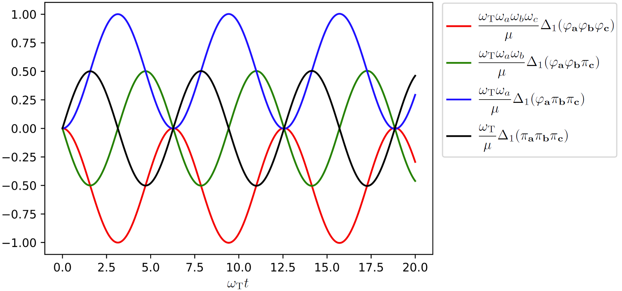
Figure 1: Evolutions of $\Delta_{1}(\varphi_{\mathbf{a}}\varphi_{\mathbf{b}}\varphi_{\mathbf{c}})$, $\Delta_{1}(\varphi_{\mathbf{a}}\varphi_{\mathbf{b}}\pi_{\mathbf{c}})$, $\Delta_{1}(\varphi_{\mathbf{a}}\pi_{\mathbf{b}}\pi_{\mathbf{c}})$, and $\Delta_{1}(\pi_{\mathbf{a}}\pi_{\mathbf{b}}\pi_{\mathbf{c}})$.

The above set forms a non-homogeneous linear ordinary differential equation system involving eight $\Delta_{1}^{(3)}$ equations with the initial condition

$$\Delta_{1}^{(3)}(t=0)=0.$$

For this initial condition, the solution is:

$$\omega_{a}\omega_{b}\omega_{c}\Delta_{1}(\varphi_{\mathbf{a}}\varphi_{\mathbf{b}}\varphi_{\mathbf{c}}) =\frac{\mu\left(\cos\omega_{\rm{T}}t-1\right)}{2\omega_{\rm{T}}}\tilde{\delta}_{\mathbf{a,b,c}},$$

$$\omega_{b}\omega_{c}\Delta_{1}(\pi_{\mathbf{a}}\varphi_{\mathbf{b}}\varphi_{\mathbf{c}}) =\omega_{c}\omega_{a}\Delta_{1}(\varphi_{\mathbf{a}}\pi_{\mathbf{b}}\varphi_{\mathbf{c}})=\omega_{a}\omega_{b}\Delta_{1}(\varphi_{\mathbf{a}}\varphi_{\mathbf{b}}\pi_{\mathbf{c}})=-\frac{\mu\sin\omega_{\rm{T}}t}{2\omega_{\rm{T}}}\tilde{\delta}_{\mathbf{a,b,c}},$$

$$\omega_{a}\Delta_{1}(\varphi_{\mathbf{a}}\pi_{\mathbf{b}}\pi_{\mathbf{c}}) =\omega_{b}\Delta_{1}(\varphi_{\mathbf{b}}\pi_{\mathbf{c}}\pi_{\mathbf{a}})=\omega_{c}\Delta_{1}(\varphi_{\mathbf{c}}\pi_{\mathbf{a}}\pi_{\mathbf{b}})=\frac{\mu(1-\cos\omega_{\rm{T}}t)}{2\omega_{\rm{T}}}\tilde{\delta}_{\mathbf{a,b,c}},$$

$$\Delta_{1}(\pi_{\mathbf{a}}\pi_{\mathbf{b}}\pi_{\mathbf{c}}) =\frac{\mu\sin\omega_{\rm{T}}t}{2\omega_{\rm{T}}}\tilde{\delta}_{\mathbf{a,b,c}},$$ (3.27)

where $\omega_{\rm{T}}=\omega_{a}+\omega_{b}+\omega_{c}$ is the inherent angular frequency of $\Delta^{(3)}$ s. The evolutions of these cubic fluctuations are depicted in Fig. 1.

These solutions demonstrate that, at the tree level in Minkowski spacetime, all $\Delta^{(3)}$ fluctuations are bounded and evolve harmonically. As discussed in Appendix B, the bounded and harmonic nature of tree-level quantum fluctuations is a characteristic feature of a Minkowski spacetime. In Section 4, we will observe that in a cosmological de Sitter spacetime, $\Delta^{(3)}_{1}$ fluctuations diverge in a $\varphi^{3}$-model as the conformal time $\eta$ approaches $0$, corresponding to the far-future of an exponentially expanding spacetime.

3.4.3 Quantum fluctuations at quantum-level

To conclude this section, we outline the typical quantum effects on the effective dynamics of the $\varphi^{3}$ model in the Minkowski spacetime. A more exhaustive study is ongoing.

We first examine the quantum effect on the classical variables $\langle\varphi_{\mathbf{a}}\rangle$ and $\langle\pi_{\mathbf{a}}\rangle$ at the $\mu^{1}$-order. Given the initial condition $\langle\varphi_{\mathbf{a}}\rangle=\langle\pi_{\mathbf{a}}\rangle=0$, their equations of motion (3.15) become:

$$\dot{\langle\varphi_{\mathbf{a}}\rangle}_{1} =\langle\pi_{\mathbf{a}}\rangle_{1},$$

$$\dot{\langle\pi_{\mathbf{a}}\rangle}_{1} =-\omega_{a}^{2}\langle\varphi_{\mathbf{a}}\rangle_{1}-\mu\int_{p}\Bigg{[}\langle\varphi_{\mathbf{p}}\rangle_{0}\langle\varphi_{\mathbf{a-p}}\rangle_{0}+\Delta_{0}(\varphi_{\mathbf{p}}\varphi_{\mathbf{a-p}})\Bigg{]}=-\omega_{a}^{2}\langle\varphi_{\mathbf{a}}\rangle_{1}-\frac{\mu}{2m}\tilde{\delta}_{\mathbf{a}}\int\frac{d^{3}k}{(2\pi)^{3}}.$$

These equations imply that $\langle\varphi_{\mathbf{a}}\rangle\neq 0$ only for $\mathbf{a}=0$. This scenario represents a homogeneous field strength $\langle\varphi(\mathbf{x})\rangle$, uniform across all positions $\mathbf{x}$. This expectation value is negative (under the assumption that $\mu>0$) and exhibits UV divergence. This divergence is anticipated, given that the $\mu\varphi^{3}$ term in the Hamiltonian, being unbounded from below, naturally pushes the field $\varphi$ towards infinite descent.

In quantum field theory, such a divergent field strength $\langle\varphi\rangle$ correlates with tadpole diagrams. Drawing from textbook quantum field theory, we know that tadpole terms break Lorentz invariance. It is conventional to redefine the field operator $\varphi$ by re-expanding it around its new expectation value $\langle\varphi\rangle$:

$$\varphi\to\varphi-\langle\varphi\rangle.$$

With this redefined field, the equations of motion for quantum fluctuations remain unchanged, resulting in

$$\langle\varphi_{\mathbf{a}}\rangle(t)=\langle\pi_{\mathbf{a}}\rangle(t)=0.$$

This is the reason for omitting the term $\Delta(\varphi_{\mathbf{k}}\varphi_{\mathbf{p}})\langle\varphi_{\mathbf{q}}\rangle$ in the fluctuation-part of the effective Hamiltonian, $H_{\text{Mink.},\Delta}$, as indicated in equation (3.6). This omission leads to the simplified form of the equations of motion presented in equation (3).

Then, as a simple yet nontrivial example, we consider an observable quantum effect — the $\mu^{2}$-order correction, $\Delta^{(2)}_{2}$, to the quadratic quantum fluctuations. Having determined all $\Delta_{1}^{(3)}$ in Eqs. (3.27), we can now express the $\mu^{2}$-order equations of motion for quadratic quantum fluctuations as follows:

$$\dot{\Delta}_{2}(\varphi_{\mathbf{a}}\varphi_{\mathbf{b}}) =\Delta_{2}(\pi_{\mathbf{a}}\varphi_{\mathbf{b}})+\Delta_{2}(\varphi_{\mathbf{a}}\pi_{\mathbf{b}}),$$

$$\dot{\Delta}_{2}(\varphi_{\mathbf{a}}\pi_{\mathbf{b}}) =\Delta_{2}(\pi_{\mathbf{a}}\pi_{\mathbf{b}})-\omega_{b}^{2}\Delta_{2}(\varphi_{\mathbf{a}}\varphi_{\mathbf{b}})-\mu\int_{p}{(2\pi)^{3}}\Delta_{1}(\varphi_{\mathbf{a}}\varphi_{\mathbf{p}}\varphi_{\mathbf{b-p}}),$$

$$=\Delta_{2}(\pi_{\mathbf{a}}\pi_{\mathbf{b}})-\omega_{b}^{2}\Delta_{2}(\varphi_{\mathbf{a}}\varphi_{\mathbf{b}})+\frac{\mu^{2}}{2}\tilde{\delta}_{\mathbf{a,b}}\int_{p}\frac{1-\cos\omega_{\rm{T}}t}{\omega_{\rm{T}}\omega_{a}\omega_{p}\omega_{|\mathbf{a+p}|}}$$

$$\dot{\Delta}_{2}(\pi_{\mathbf{a}}\pi_{\mathbf{b}}) =-\omega_{a}^{2}\Delta_{2}(\varphi_{\mathbf{a}}\pi_{\mathbf{b}})-\omega_{b}^{2}\Delta_{2}(\varphi_{\mathbf{a}}\pi_{\mathbf{b}})-\mu\int_{p}\left[\Delta_{1}(\pi_{\mathbf{a}}\varphi_{\mathbf{p}}\varphi_{\mathbf{b-p}})+\Delta_{1}(\pi_{\mathbf{b}}\varphi_{\mathbf{p}}\varphi_{\mathbf{a-p}})\right]$$

$$=-\omega_{a}^{2}\Delta_{2}(\varphi_{\mathbf{a}}\pi_{\mathbf{b}})-\omega_{b}^{2}\Delta_{2}(\varphi_{\mathbf{a}}\pi_{\mathbf{b}})+\mu^{2}\tilde{\delta}_{\mathbf{a,b}}\int_{p}\frac{\sin\omega_{\rm{T}}t}{\omega_{\rm{T}}\omega_{a}\omega_{|\mathbf{a+p}|}},$$

where

$$\omega_{\rm{T}}=\omega_{a}+\omega_{p}+\omega_{\mathbf{|\mathbf{a+p}|}}.$$

The RHS of these equations exhibit $\ln\Lambda$ UV divergence, where $\Lambda$ is the UV cutoff. Renormalization is necessary to address this divergence, resulting in $\mu^{2}$-order corrections to quadratic $\Delta^{(2)}_{0}$ in (3.24). The renormalization procedure remains a subject of ongoing investigations.

4 Fields on cosmological spacetimes

We have seen in the previous section that our framework can provide a consistent effective description of quantum fields in flat spacetime. The description allowed for analytical solutions to the $\varphi^{3}$-model without relying on any operator-method input..

For cosmological spacetimes, such as the exponentially expanding spacetime of inflation, solving the effective equations for an interacting field is not easy. Results from the in-in method [30] already suggest that for cubic fluctuations, the solution can at best only be written in terms of non-elementary complex integrals that integrate to the (conformal) time of interest $\eta$. It is only in the superhorizon limit can one hope to express the solutions in terms of elementary functions.

In our effective framework, we will soon see the obstruction to obtaining analytical solutions manifest in the form of time-dependent interaction strengths. In the $\varphi^{3}$-model on de Sitter, these will appear as functions $\Omega_{k}^{2}(\eta)$ for the quadratic interaction and $\lambda(\eta)$ for the cubic interaction. The analogue of (3.14) in an expanding spacetime will typically not be solvable analytically when these interaction strengths depend on $\eta$.

Fortunately, following the strategy outlined in Section 3.4, one could still numerically describe the evolution of 3-pt correlators. One simply needs to organize the solution in cubic-interaction strength and use the uncertainty principle to find the desired minimal-energy initial conditions. At the zeroth-order in cubic-interaction strength, the analogue of (3.13) can still be solved analytically despite the quadratic-interaction strength being time-dependent. As we will see, however, this process sees additional subtleties. The expansion of spacetime permits different choices of canonical variables that correspond to different minimal-energy initial conditions, even at the zeroth-order in cubic-interaction strength . The differences vanish if one sets initial conditions at past-infinity. But for inflation, it has been debated whether too much expansion could lead to the “trans-Planckian” problem [31]. Settling the debate is beyond the scope of this work. For demonstration purposes, we will instead simply pick a set of canonical variables to show that our effective framework is self-consistent and that one could arrive at the correct value for the cubic fluctuation $\Delta(\delta\varphi\delta\varphi\delta\varphi)$ (in the superhorizon limit) when compared with the in-in method outlined in [32].

4.1 Free field

Let us warm up by analyzing a free field on a fixed de Sitter background. The action of such a system is

$$S_{2}=\int d\eta d^{3}x\frac{1}{2}\sqrt{|g|}\Big{[}-g^{\mu\nu}\partial_{\mu}\varphi\partial_{\nu}\varphi\Big{]}\,.$$ (4.1)

We can split the field into a background (homogeneous) part and a perturbation (inhomogeneous) part

$$\varphi(\eta,\mathbf{x})=\bar{\varphi}(\eta)+\delta\varphi(\eta,\mathbf{x})\,.$$

Substituting this separation into action (4.1), and upon imposing the background equations of motion (for $\bar{\varphi}(\eta)$), the $O(\delta\varphi)$ term vanishes. We thus have an action where perturbation decouples from the background system

$$S_{2}|_{\mathrm{OS}}=\int d\eta d^{3}xa^{2}\frac{1}{2}\bar{\varphi}^{2}+\int d\eta d^{3}xa^{2}\frac{1}{2}\Big{[}(\delta\varphi^{\prime})^{2}-\frac{1}{2}\delta^{ij}\partial_{i}\delta\varphi\partial_{j}\delta\varphi\Big{]}\,,$$

where the subscript “$\mathrm{OS}$” means on-shell for the background system.

Now consider the $O(\delta\varphi^{2})$-part of the action

$$S_{\mathrm{Free}}=\int d\eta d^{3}xa^{2}\Big{[}\frac{1}{2}(\delta\varphi^{\prime})^{2}-\frac{1}{2}\delta^{ij}\partial_{i}\delta\varphi\partial_{j}\delta\varphi\Big{]}\,,$$ (4.2)

which we call the “free” part to separate it from the interacting part consisting of $O(\delta\varphi^{3})$-order and higher. (We wish to emphasize that the notion of the “free” part is ambiguous when there are $\delta\varphi^{\prime}$-type interactions, but it is not an issue here.)

The prescription for obtaining an effective Hamiltonian and its equations of motion is similar to the one outlined in Section 3. But there is a nuance in the case of a cosmological spacetime: There are at least three “natural” sets of canonical variables [22]. We must choose one before we can begin canonical quantization. Different choices cannot be expected to be physically equivalent [33], as we now address.

4.1.1 Different choices of variables and initial conditions

We claim that there are three “natural” sets of configuration variables because of two observations. First, canonically quantizing (4.2) “as is” and imposing an initial vacuum (associated with $\eta$-time slicing) lead to divergences at early times, which may make quantization inconsistent. Second, action (4.2) is not one that collects the familiar simple harmonic oscillators in Fourier space due to the $a^{2}$ factor. If one ignores these two issues, one could insist that the variables $\delta\varphi$ and $\pi=a^{2}\delta\varphi^{\prime}$ are natural and carry out the standard canonical quantization. Otherwise, one could find two other sets of variables, which we now introduce.

At the present level, the two issues highlighted above are mostly aesthetic, assuming that one imposes initial conditions at past infinity ($\eta\rightarrow-\infty$). The observables will not be affected. (Nevertheless, the situation will worsen a lot for generic non-Gaussian systems.) One might be tempted to make the system appear more like harmonic oscillators and its initial conditions more convergent with a change of variables to $f=a\delta\varphi$. The “$f$-variable” enables us to do two things. One, we can trade initial divergences for late-time divergences. The late time divergences are not as problematic because the system will have classicalized and one would not have to deal with infinities in Hilbert space. The correlators associated with $\delta\varphi$ will also remain finite. Two, we may refurbish our system into simple harmonic oscillators with one catch: We need to integrate by parts. The act of integration by parts affects nothing if one imposes quantum initial conditions at past infinity. But the situation will be different otherwise.

Let us be more specific. The first of the three natural variables we can pick is the original $\delta\varphi$ and its canonical momentum $\pi_{\delta\varphi}=\delta\varphi^{\prime}$. The other two options arise after changing to the variable $f=a\delta\varphi$. After switching to $f$-variables, one is faced with two possible actions, differentiated by our willingness to ignore a boundary term

$$\text{Option 1: }S_{\mathrm{free},1}=\int d\eta d^{3}x\frac{1}{2}\Big{[}(f^{\prime})^{2}-2\mathcal{H}ff^{\prime}+\mathcal{H}^{2}f^{2}-\delta^{ij}\partial_{i}f\partial_{j}f\Big{]}$$

$$\text{Canonical momentum: }\pi_{1}(\eta,\mathbf{x})=f^{\prime}(\eta,\mathbf{x})-\mathcal{H}f$$

$$\text{Option 2: }S_{\mathrm{free},2}=\int d\eta d^{3}x\frac{1}{2}\Big{[}(f^{\prime})^{2}+\frac{a^{\prime\prime}}{a}f^{2}-\delta^{ij}\partial_{i}f\partial_{j}f\Big{]}-\cancel{\frac{1}{2}\int d\eta d^{3}x(\mathcal{H}f^{2})^{\prime}}$$

$$\text{Canonical momentum: }\pi_{2}(\eta,\mathbf{x})=f^{\prime}(\eta,\mathbf{x})\,,$$ (4.3)

where $\mathcal{H}=a^{\prime}/a$ is the Hubble parameter in conformal time. The two options will introduce two distinct canonical momenta due to differences in terms with “velocity” $f^{\prime}$ in the Lagrangian.

The action from option 1 is completely equivalent to the original one (4.2), whereas the action from option 2 — which ignores the boundary term — resembles a set of simple harmonic oscillators, albeit with time-dependent “frequencies”. So in terms of picking a “natural” starting point for canonical quantization, neither of the options offers a significant merit over the other.

Does this mean one can pick any one of the two options? No, unless one sets initial conditions at past infinity. If one follows the standard canonical quantization and assumes an initial minimal-energy or Gaussian state (which includes the usual Bunch-Davies vacuum), what matters are the initial values for the quadratic expectation values

$$\langle ff\rangle\,,\;\langle f\pi\rangle\,,\;\langle\pi\pi\rangle\,,$$ (4.4)

where the $\pi$ above can be either $\pi_{1}$ or $\pi_{2}$. Clearly, since $\pi_{2}-\pi_{1}=\mathcal{H}f\sim-\eta^{-1}$ on de Sitter, the differences in quadratic expectation values for the two choices of momentum vanish only when $\eta\rightarrow-\infty$ at past infinity. (The situation will worsen when there is a “velocity” type non-Gaussian terms in the Lagrangian — the differences in initial expectation values may even diverge for different choices of canonical momentum.)

Our effective framework offers a more intuitive way to understand the discrepancy: Different canonical pairs correspond to different effective Hamiltonians, and hence, different minimal-energy conditions. In our case, the differences in minimal energy states vanish in the infinite-past limit.

In Fourier space, by applying our prescription for obtaining the effective Hamiltonian, we have

$$\text{Option 1: }H_{1,\Delta}=\int_{k}\Big{[}\frac{1}{2}\Delta(\pi_{1,\mathbf{k}}\pi_{1,\mathbf{-k}})+\mathcal{H}\Delta(f_{\mathbf{k}}\pi_{1,\mathbf{-k}})+\frac{1}{2}k^{2}\Delta(f_{\mathbf{k}}f_{\mathbf{-k}})\Big{]}$$

$$\text{Option 2: }H_{2,\Delta}=\int_{k}\Big{[}\frac{1}{2}\Delta(\pi_{2,\mathbf{k}}\pi_{2,\mathbf{-k}})+\frac{1}{2}(k^{2}+\frac{a^{\prime\prime}}{a})\Delta(f_{\mathbf{k}}f_{\mathbf{-k}})\Big{]}\,.$$

In de Sitter, both $a^{\prime\prime}/a$ and $\mathcal{H}$ vanish in the infinite-past limit ($\eta\rightarrow-\infty$), so the difference between the two effective Hamiltonians vanishes. One can use our uncertainty-principle prescription in Section 3.3 to find a common set of initial values for the two options — they correspond to the Minkowski vacuum in the operator/Hilbert-space Language. This is what modes feel in the subhorizon limit under Bunch-Davies initial conditions because their scales are too small to feel any effects from curvature.

But for a finite initial time $|\eta_{i}|<\infty$, there is no common set of initial values for the two options anymore. To find their minimal-energy conditions, one should use the uncertainty principle, per Section 3.3. The prescription outlined there tells us that the minima of the two Hamiltonians are

$$\text{Option 1: }H_{1,\Delta}\geq\int_{k}\Big{[}\mathcal{H}\Delta(f_{\mathbf{k}}\pi_{1,\mathbf{-k}})+k\sqrt{\Delta^{2}(f_{\mathbf{k}}\pi_{1,\mathbf{-k}})+\frac{1}{4}\tilde{\delta}(\mathbf{0})^{2}}\Big{]}\,.$$

$$\text{Option 2: }H_{2,\Delta}\geq\int_{k}\Big{[}(k^{2}-\frac{2}{\eta^{2}})^{1/2}\sqrt{\Delta^{2}(f_{\mathbf{k}}\pi_{2,\mathbf{-k}})+\frac{1}{4}\tilde{\delta}(\mathbf{0})^{2}}\Big{]}\,.$$

Note that $1/4\tilde{\delta}(\mathbf{0})^{2}\rightarrow\hbar^{2}/4\tilde{\delta}(\mathbf{0})^{2}$ if we restore $\hbar$, and $\tilde{\delta}(\mathbf{0})$ comes from $\tilde{\delta}(\mathbf{k-k})$. The smallest values of the two lower bounds are reached when

Option 1: $$k^{2}\Delta(f_{\mathbf{k}}f_{\mathbf{-k}})=\Delta(\pi_{1,\mathbf{k}}\pi_{1,\mathbf{-k}})=k\sqrt{\Delta^{2}(f_{\mathbf{k}}\pi_{1,\mathbf{-k}})+\frac{1}{4}\tilde{\delta}(\mathbf{0})^{2}}\,,\;$$

$$\Delta^{2}(f_{\mathbf{k}}\pi_{1,\mathbf{-k}})=\frac{1}{4}\frac{1}{(k/\mathcal{H})^{2}-1}\tilde{\delta}(\mathbf{0})^{2}\,.$$

Option 2: $$(k^{2}-\frac{2}{\eta^{2}})\Delta(f_{\mathbf{k}}f_{\mathbf{-k}})=\Delta(\pi_{2,\mathbf{k}}\pi_{2,\mathbf{-k}})=(k^{2}-\frac{2}{\eta^{2}})^{1/2}\sqrt{\Delta^{2}(f_{\mathbf{k}}\pi_{2,\mathbf{-k}})+\frac{1}{4}\tilde{\delta}(\mathbf{0})^{2}}\,,\;$$

$$\Delta^{2}(f_{\mathbf{k}}\pi_{2,\mathbf{-k}})=0\,.$$ (4.5)

In particular, when the effective Hamiltonians are minimized, the initial 2-pt functions,

$$\Delta(f_{\mathbf{k}}f_{\mathbf{-k}})|_{\text{option 1}}=\frac{1}{2}(k^{2}-\frac{1}{\eta_{i}^{2}})^{-1/2}\tilde{\delta}(\mathbf{0})\,,\;\Delta(f_{\mathbf{k}}f_{\mathbf{-k}})|_{\text{option 2}}=\frac{1}{2}(k^{2}-\frac{2}{\eta_{i}^{2}})^{-1/2}\tilde{\delta}(\mathbf{0})\,,$$ (4.6)

differ, significantly for long-wavelength modes. Nevertheless, they coincide when the initial time is taken to the $\eta_{i}\rightarrow-\infty$ limit.

Suppose one demands that the effective system (for either option 1 or option 2) rests in its minimal-energy configuration initially according to (4.5). Not all modes “feel” a Minkowski vacuum, as is commonly assumed in an operator/Hilbert-space framework [34]. The modes are actually in squeezed states [35], where the squeezing parameter depends on both the wavenumber $k$ and initial time $\eta_{i}$ in a non-polynomial way.

The use of non-Bunch-Davies initial conditions has observational consequences. This was discussed in [22] by employing different canonical variables and using an operator/Hilbert-space language. Alternatively, our effective framework provides an easier parameterization of initial conditions using quantum fluctuations as dynamical quantities. As a potential application in this direction, we would like to point out the possibility of explaining the large-angle anomaly in the CMB [36]. We see, for example in (4.6), that large-wavenumber modes deviate from the Minkowski vacuum the most. To explain the weakness of large-angle temperature correlations, we would require modes with large wavenumbers to contribute weaker power spectra compared with the standard Bunch-Davies result. In [22], squeezed initial conditions akin to (4.5) lead to a modified power spectrum that is ambiguous in whether it amplifies or weakens the large-angle sector of the power spectrum. So a squeezed initial state may not be enough to explain the anomaly. Using our method, however, one could parameterize more general hierarchies between fluctuations in an $\eta_{i}$- or $k$-dependent way. The ratio between the fluctuations $\Delta(ff)$ and $\Delta(\pi\pi)$, such as the ones in (4.5), are among the simplest parameterizations of a fluctuation-hierarchy — Our method provides a way to probe more complicated ones, potentially involving higher-order fluctuations. The examination of CBM anomalies using our effective framework is the subject of an ongoing investigation, which will be reported elsewhere.

4.1.2 The equations of motion and its solution

To demonstrate our effective framework without having to worry about ambiguity in variables, we will assume that initial conditions can be set at past infinity so that we are free to pick any one of the aforementioned canonical momenta. We will use option 2 in (4.3) for easier comparison with the flat-spacetime case of Section 3. That is, our effective Hamiltonian in Fourier space will be

$$H_{\mathrm{free},\Delta}=\int_{k}\frac{1}{2}\Big{[}\Delta(\pi_{\mathbf{k}}\pi_{\mathbf{-k}})+\Omega_{k}^{2}(\eta)\Delta(f_{\mathbf{k}}f_{\mathbf{-k}})\Big{]}\,,\;\pi_{\mathbf{k}}=f^{\prime}_{\mathbf{k}}\,,\;\Omega_{k}^{2}(\eta)=k^{2}-\frac{2}{\eta^{2}}\,,$$ (4.7)

where we have used a fixed de Sitter solution for $a^{\prime\prime}/a$.

To obtain initial conditions we again assume that the initial fluctuations follow a Gaussian hierarchy (where Wick’s theorem applies) and minimizes $H_{\mathrm{free},\Delta}$. The only initial free parameters we must find are the quadratic expectation values, which can be found with the uncertainty-principle prescription as before

$$\Delta(f_{\mathbf{p}}\pi_{\mathbf{q}})= 0\times\tilde{\delta}_{\mathbf{p,q}}$$

$$\Delta(f_{\mathbf{p}}f_{\mathbf{q}})= \frac{1}{2p}\tilde{\delta}_{\mathbf{p,q}}$$

$$\Delta(\pi_{\mathbf{p}}\pi_{\mathbf{q}})= \frac{p}{2}\tilde{\delta}_{\mathbf{p,q}}\,.$$ (4.8)

They look exactly like the Minkowski version, as is expected from a Bunch-Davies initial condition in the subhorizon limit.

With the Poisson bracket rules for the fluctuations, we can derive the equations of motion for $H_{\mathrm{free},\Delta}$ to be

$$\Delta^{\prime}(f_{\mathbf{p}}f_{\mathbf{q}})= \Delta(f_{\mathbf{p}}\pi_{\mathbf{q}})+\Delta(f_{\mathbf{q}}\pi_{\mathbf{p}})$$

$$\Delta^{\prime}(f_{\mathbf{p}}\pi_{\mathbf{q}})= \Delta(\pi_{\mathbf{p}}\pi_{\mathbf{q}})-\Omega_{q}^{2}(\eta)\Delta(f_{\mathbf{p}}f_{\mathbf{q}})$$

$$\Delta^{\prime}(\pi_{\mathbf{p}}\pi_{\mathbf{q}})= -\Omega_{q}^{2}(\eta)\Delta(\pi_{\mathbf{p}}f_{\mathbf{q}})-\Omega_{p}^{2}(\eta)\Delta(\pi_{\mathbf{q}}f_{\mathbf{p}})\,.$$ (4.9)

When one assumes statistical homogeneity and isotropy, the quadratic expectation values above are delta-functions times real functions of $\eta$. Imposing our initial conditions, these equations of motion can be solved by hand to be

$$\Delta(f_{\mathbf{p}}f_{\mathbf{q}})= \Big{(}\frac{1}{2p}+\frac{1}{2p^{3}\eta^{2}}\Big{)}\tilde{\delta}_{\mathbf{p,q}}$$

$$\Delta(f_{\mathbf{p}}\pi_{\mathbf{q}})= -\frac{1}{2(p\eta)^{3}}\tilde{\delta}_{\mathbf{p,q}}$$

$$\Delta(\pi_{\mathbf{p}}\pi_{\mathbf{q}})= \Big{(}\frac{p}{2}-\frac{1}{2p\eta^{2}}+\frac{1}{2p^{3}\eta^{4}}\Big{)}\tilde{\delta}_{\mathbf{p,q}}\,.$$ (4.10)

These solutions coincide with the expectation values obtained in an operator formalism, assuming Bunch-Davies initial conditions.

In particular, in the spatially-flat gauge, the comoving curvature perturbation $\mathcal{R}$ and the perturbation $\delta\varphi$ are related by

$$\mathcal{R}=\frac{\mathcal{H}}{\bar{\varphi}^{\prime}}\delta\varphi\,.$$

This gives the power spectrum of $\mathcal{R}$ to be

$$\langle\mathcal{R}_{\mathbf{p}}\mathcal{R}_{\mathbf{q}}\rangle=(\frac{\mathcal{H}}{a\bar{\varphi}^{\prime}})^{2}\langle f_{\mathbf{p}}f_{\mathbf{q}}\rangle\longrightarrow\frac{H^{2}}{\dot{\bar{\varphi}}^{2}}\frac{H^{2}}{2p^{3}}(2\pi)^{3}\delta^{3}(\mathbf{p+q})\,,$$ (4.11)

where the arrow indicates the superhorizon limit.

4.2 Interacting field: non-Gaussianities

In this section, we apply our formalism to the case of an interacting field on fixed de Sitter background. This system serves as a good approximation if one considers up to leading order in slow roll and assumes sufficient decoupling between metric and matter perturbations. Our goal is to compute the 3-pt function, or non-Gaussianity, of the theory. In passing, we demonstrate that our method is self-contained in the sense that nothing (from equations of motion to initial values to solution schemes) necessarily requires any operator-formalism input. The techniques developed in Section 3 suffice.

Let us first consider a generic matter action with potential $V(\varphi)$

$$S[\varphi]=\int d\eta d^{3}x\sqrt{|g|}\Big{[}-\frac{1}{2}g^{\mu\nu}\partial_{\mu}\varphi\partial_{\nu}\varphi-V(\varphi)\Big{]}\,.$$ (4.12)

We will again assume the following splitting and change of variables

$$\varphi(\eta,\mathbf{x})=\bar{\varphi}(\eta)+\delta\varphi(\eta,\mathbf{x})\,,\;f=a\delta\varphi(\eta,\mathbf{x})\,.$$ (4.13)

The action can then be split into a background part, containing only $\bar{\varphi}$, and perturbation part containing terms $O(f^{2},f^{3})$ or higher.

$$S[\varphi]|_{\mathrm{OS}}=S_{0}[\bar{\varphi}]+\int d\eta d^{3}x[\frac{1}{2}(f^{\prime})^{2}+\frac{1}{2}(\frac{2}{\eta^{2}}f^{2}-\delta^{ij}\partial_{i}f\partial_{j}f)-a^{4}\sum_{n=2}\frac{1}{n!}(\partial_{\phi}^{(n)}V)|_{\phi_{0}}(\frac{f}{a})^{n}]$$ (4.14)

To arrive at the above action, we have imposed the equation of motion for the background field $\bar{\varphi}$, as implied by the subscript “$\mathrm{OS}$” for on-shell. This makes terms linear in $\delta\varphi$ vanish and explains why the sum in the integration starts at $n=2$. Additionally, integration by parts is performed.

Now, consider the case for $V(\varphi)=\lambda_{0}\varphi^{3}/3$ where $\lambda_{0}$ is a time-dependent small parameter controlling the magnitude of non-Gaussianity. (The smallness is also necessary from the point of view of background spacetime stability.) Up to leading order in slow-roll, the $V_{\varphi\varphi}$ term in (4.14) is negligible compared to other terms, giving us the action

$$S[\varphi]|_{\mathrm{OS}}\approx S_{0}[\bar{\varphi}]+\int d\eta d^{3}x\Bigg{[}\frac{1}{2}(f^{\prime})^{2}+\frac{1}{2}\Big{(}\frac{2}{\eta^{2}}f^{2}-\delta^{ij}\partial_{i}f\partial_{j}f\Big{)}+\frac{\lambda_{0}}{3H}\frac{1}{\eta}f^{3}\Bigg{]}\,.$$ (4.15)

Viewed in Fourier space, the action resembles that of a $\varphi^{3}$-model on flat spacetime but with an effective time-dependent mass and cubic-interaction (for a mode with wavenumber $k=|\mathbf{k}|$)

$$\Omega_{k}^{2}(\eta)=k^{2}-\frac{2}{\eta^{2}}\,,\;\lambda(\eta)=-\frac{\lambda_{0}}{H\eta}.$$ (4.16)

The sign change for the coupling strength is due to the translation from the scale factor to conformal time, $a(\eta)=-1/(\eta H)$, on fixed de Sitter.

To apply our formalism to the system (4.15), we first notice that its $O(f^{2},f^{3})$-part does not “backreact” on $S_{0}[\bar{\varphi}]$ in the sense that $\bar{\varphi}$ and $f$ do not mix in the Lagrangian and the background spacetime is fixed regardless of how $f$ evolves. So in a Hamiltonian formalism, we only need to examine the $O(f^{2},f^{3})$-part of the action if we are only interested in the evolution of $f$.

Thus the Lagrangian and Hamiltonian governing variable $f$ are (in the Fourier space)

$$S_{f^{3}}\equiv S[\varphi]|_{\mathrm{OS}}-S_{0}[\bar{\varphi}]$$

$$= \int d\eta\int_{k}\Big{[}\frac{1}{2}f^{\prime}_{\mathbf{k}}f^{\prime}_{\mathbf{-k}}+\frac{1}{2}\Omega_{k}^{2}(\eta)f_{\mathbf{k}}f_{\mathbf{-k}}\Big{]}$$

$$+ \int d\eta\int_{k,p,q}\frac{\lambda(\eta)}{3}f_{\mathbf{k}}f_{\mathbf{p}}f_{\mathbf{q}}\tilde{\delta}_{\mathbf{k,p,q}}\,,$$

$$H_{f^{3}}= \int d\eta\int_{k}\Big{[}\frac{1}{2}\pi_{\mathbf{k}}\pi_{\mathbf{-k}}+\frac{1}{2}\Omega_{k}^{2}(\eta)f_{\mathbf{k}}f_{\mathbf{-k}}\Big{]}$$

$$+ \int d\eta\int_{k,p,q}\frac{\lambda(\eta)}{3}f_{\mathbf{k}}f_{\mathbf{p}}f_{\mathbf{q}}\tilde{\delta}_{\mathbf{k,p,q}}\,.$$

Since there are no velocity-type interactions, the canonical conjugate to $f_{\mathbf{k}}$ is simply $\pi_{\mathbf{k}}=f^{\prime}_{\mathbf{k}}$, with Fourier-space normalization $\{f_{\mathbf{k}},\pi_{\mathbf{p}}\}=\tilde{\delta}_{\mathbf{k,p}}$.

Upon employing our effective formalism, the fluctuation part of the effective Hamiltonian is

$$H_{\Delta}[H_{f^{3}}]\equiv H_{Q}[H_{f^{3}}]-H_{0}[H_{f^{3}}]$$

$$= \frac{1}{2}\int_{k}\Big{[}\Delta(\pi_{\mathbf{k}}\pi_{\mathbf{-k}})+\Omega_{k}^{2}(\eta)\Delta(f_{\mathbf{k}}f_{\mathbf{-k}})\Big{]}$$

$$+ \int_{k,p,q}\frac{\lambda(\eta)}{3}\Big{[}3\Delta(f_{\mathbf{k}}f_{\mathbf{p}})\langle f_{\mathbf{k}}\rangle+\Delta(f_{\mathbf{k}}f_{\mathbf{p}}f_{\mathbf{q}})\Big{]}\tilde{\delta}_{\mathbf{k,p,q}}\,,$$ (4.17)

where we have re-shuffled the integration variables to get the factor of the $O(\langle f\rangle)$ term in the third line.

For solutions respecting translational and rotational invariance on the level of quantum averages, linear-operator expectation values like $\langle f_{\mathbf{k}}\rangle,\langle\pi_{\mathbf{k}}\rangle$ will vanish. The cubic-$\Delta$ equations of motion are therefore

$$\Delta^{\prime}(f_{\mathbf{b}}f_{\mathbf{c}}f_{\mathbf{d}})= \Delta(f_{\mathbf{b}}f_{\mathbf{c}}\pi_{\mathbf{d}})+\Delta(f_{\mathbf{c}}f_{\mathbf{d}}\pi_{\mathbf{b}})+\Delta(f_{\mathbf{d}}f_{\mathbf{b}}\pi_{\mathbf{c}})$$

$$\Delta^{\prime}(f_{\mathbf{b}}f_{\mathbf{c}}\pi_{\mathbf{d}})= \Delta(f_{\mathbf{b}}\pi_{\mathbf{c}}\pi_{\mathbf{d}})+\Delta(f_{\mathbf{c}}\pi_{\mathbf{b}}\pi_{\mathbf{d}})-\Omega_{d}^{2}(\eta)\Delta(f_{\mathbf{b}}f_{\mathbf{c}}f_{\mathbf{d}})$$

$$+ \lambda(\eta)\int_{k,p,q}\tilde{\delta}_{\mathbf{k,p,q}}(-\tilde{\delta}_{\mathbf{d},\mathbf{k}})[\Delta(f_{\mathbf{b}}f_{\mathbf{c}}f_{\mathbf{p}}f_{\mathbf{q}})-\Delta(f_{\mathbf{p}}f_{\mathbf{q}})\Delta(f_{\mathbf{b}}f_{\mathbf{c}})]$$

$$\Delta^{\prime}(f_{\mathbf{b}}\pi_{\mathbf{c}}\pi_{\mathbf{d}})= \Delta(\pi_{\mathbf{b}}\pi_{\mathbf{c}}\pi_{\mathbf{d}})-[\Omega_{c}^{2}(\eta)\Delta(f_{\mathbf{b}}f_{\mathbf{c}}\pi_{\mathbf{d}})+(\mathbf{c}\leftrightarrow\mathbf{d})]$$

$$+ \lambda(\eta)\int_{k,p,q}\tilde{\delta}_{\mathbf{k,p,q}}[-\tilde{\delta}_{\mathbf{c,k}}(\Delta(f_{\mathbf{b}}f_{\mathbf{p}}f_{\mathbf{q}}\pi_{\mathbf{d}})-\Delta(f_{\mathbf{b}}\pi_{\mathbf{d}})\Delta(f_{\mathbf{p}}f_{\mathbf{q}}))+(\mathbf{c}\leftrightarrow\mathbf{d})]$$

$$\Delta^{\prime}(\pi_{\mathbf{b}}\pi_{\mathbf{c}}\pi_{\mathbf{d}})= -\Omega_{b}^{2}(\eta)\Delta(f_{\mathbf{b}}\pi_{\mathbf{c}}\pi_{\mathbf{d}})-\Omega_{c}^{2}(\eta)\Delta(f_{\mathbf{c}}\pi_{\mathbf{d}}\pi_{\mathbf{b}})-\Omega_{d}^{2}(\eta)\Delta(f_{\mathbf{d}}\pi_{\mathbf{b}}\pi_{\mathbf{c}})$$

$$+ \lambda(\eta)\int_{k,p,q}\tilde{\delta}_{\mathbf{k,p,q}}\Big{[}-\tilde{\delta}_{\mathbf{b,k}}(\Delta(\pi_{\mathbf{c}}\pi_{\mathbf{d}}f_{\mathbf{p}}f_{\mathbf{q}})-\Delta(\pi_{\mathbf{c}}\pi_{\mathbf{d}})\Delta(f_{\mathbf{p}}f_{\mathbf{q}}))$$

$$+ (\text{Two more terms cycling }\mathbf{b\rightarrow c\rightarrow d})\Big{]}$$

$$+ \frac{1}{2}\lambda(\eta)\tilde{\delta}_{\mathbf{b,c,d}}\,.$$ (4.18)

These equations look formally like the equations of motion (3.14) for the $\varphi^{3}$-model on Minkowski but with a time-dependent mass and cubic-interaction parameter.

4.2.1 Finding the solution

We will try to solve the cubic fluctuations perturbatively in $O(\lambda)$. Given a Gaussian initial condition, the cubic fluctuations vanish in $O(\lambda^{0})$. So to find the leading order non-trivial solution, we only need to go to $O(\lambda)$. What this means for the equation set (4.18) is that the even-order fluctuations inside integrals only need to be kept up to $O(\lambda^{0})$, i.e., its “free” solution.

Previously, the free solution is

$$\Delta(f_{\mathbf{k}}f_{\mathbf{p}})= \Big{(}\frac{1}{2k}+\frac{1}{2k^{3}\eta^{2}}\Big{)}\tilde{\delta}_{\mathbf{k,p}}$$

$$\Delta(f_{\mathbf{k}}\pi_{\mathbf{p}})= -\frac{1}{2(k\eta)^{3}}\tilde{\delta}_{\mathbf{k,p}}$$

$$\Delta(\pi_{\mathbf{k}}\pi_{\mathbf{p}})= \Big{(}\frac{k}{2}-\frac{1}{2k\eta^{2}}+\frac{1}{2k^{3}\eta^{4}}\Big{)}\tilde{\delta}_{\mathbf{k,p}}\,,$$

with all other fluctuations obtained via a Gaussian hierarchy, which in particular means that all odd-order fluctuations vanish.

With the initial values determined and free solutions specified, one can solve the cubic order fluctuations up to $O(\lambda)$. Because of the time dependence in $\Omega_{b}^{2}(\eta)$ and $\lambda(\eta)$, the solutions cannot be obtained analytically. We therefore use numerical evolution. The result for the 3-pt correlator $\langle\delta\varphi_{\mathbf{b}}\delta\varphi_{\mathbf{c}}\delta\varphi_{\mathbf{c}}\rangle$ is shown in Figure 2, where we also make the comparison with the superhorizon-limit expression obtained from the “in-in” method.

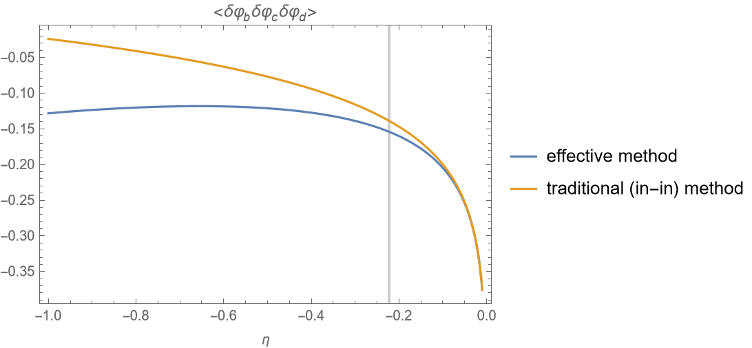
Figure 2: The comparison between the solution to (4.18) (blue) and the superhorizon limit of the ”in-in” result (yellow). (Namely, the accuracy of the yellow line in representing the 3-pt correlator becomes worse as one extends back into the subhorizon limit, or equivalently, larger $|\eta|$.) The gray vertical line represents the time of horizon crossing for the mode $k_{\mathrm{T}}\equiv|\mathbf{b}|+|\mathbf{c}|+|\mathbf{d}|$, which roughly acts as an effective wavenumber for the 3-pt correlator. The free solution used in (4.18) are that of (4.10), which reduces in the far-past to the Bunch-Davies initial condition commonly used for the “in-in” method. The external momenta used were $(\mathbf{b,c,d})=(H,2H,1.5H)$, where $H$ is the Hubble parameter. We have checked that other sets of external momenta also exhibits excellent agreement with the “in-in” result.

Our numerical evolution shows excellent agreement with the “in-in” method in the superhorizon limit, which exhibits a $\log[-(a+b+c)\eta]$ divergence originating from the fixed de Sitter background. For more realistic cosmological applications, we would treat gauge symmetry and the weak time dependence of the Hubble parameter more seriously. The 3-pt correlator of gauge-invariant variables would then be finite and slow-roll suppressed for most single-field inflation models.

5 Conclusions and discussions

We have introduced a systematic framework for describing a quantum-field system in an effective way, without invoking an operator-Hilbert space language. The effective description, originally developed in [1] for quantum mechanical systems, treats fluctuations $\Delta$ of canonical pairs as messengers of quantum effects. Via effective Poisson brackets (2.1), one obtains an effective Hamiltonian that governs the evolution of fluctuations. This provides us with a time-dependent description of how quantum fluctuations backreact on the classical part of the system. At second order in fluctuations, minimizing the effective Hamiltonian while respecting the uncertainty principle leads to the Coleman-Weinberg effective potential, which can be understood as a low-energy limit of the $H_{\Delta}$ that we constructed. We have shown that this way of obtaining the low-energy effective potential works for both quantum mechanics and quantum fields. In particular, the saturation of minimal uncertainty becomes a result rather than an assumption when one wishes to find the low-energy effective potential.

The novel part of our work lies in showing how one could go beyond the low-energy effective potential for interacting field systems by allowing fluctuations to evolve freely instead of taking fixed values that minimize energy. At first glance, a field system would give rise to infinitely many equations of motion for the fluctuations. By arguing from the perspective of minimal backreaction, we have motivated the use of translational and rotational symmetries and shown how to make finite the number of equations. Physically, we have thus shown that minimal backreaction helps maintain spatial symmetries, which decouple the evolution of fluctuations from both themselves and the inhomogeneous part of the classical background.

In flat space, one could even find analytical solutions by hand following the strategy outlined in Section 3. The key elements used were: (1) perturbation theory (in interaction strength); (2) a set of minimal-energy initial conditions found using the uncertainty principle; (3) an initial Gaussian hierarchy where Wick’s theorem applies. These three elements are also manifest in the core techniques of textbook quantum field theory — perturbation around a Gaussian system and the assumption of initial “free” vacuum, which together imply Wick’s theorem. In our framework, the three key elements are enough to completely fix the system of equations, allowing us to solve for the fluctuations by hand. We have demonstrated this with a $\varphi^{3}$-model. But the strategy also applies to systems with more generic interactions, even on curved spacetimes.

In particular, we have shown that for a $\varphi^{3}$-model on a de Sitter background our result for the 3-pt correlator (or bispectrum) agrees with the “in-in” result in the superhorizon limit. This gives us confidence to apply it to more realistic inflationary systems, with more complicated interactions and additional subtleties arising from gauge invariance. The systematic application of our method to the calculation of non-Gaussianities will be left for future work. We end by mentioning some opportunities and challenges in this direction.

Backreaction and stability of the background. Our framework naturally incorporates how time-dependent quantum fluctuations backreact on classical field variables. A preliminary investigation in this direction, using toy models and an approximate canonical map for second-order fluctuations, was carried out in [16]. In our work, we have extended the investigation to higher-order fluctuations for interacting fields on static and expanding backgrounds. We have shown that backreaction is minimized when spatially symmetric initial conditions are used. Nevertheless, the stability of spatial symmetries to quantum backreaction remains to be explored.

For inflationary cosmology, one could envision a scenario where a small deviation from initial homogeneity and isotropy causes the inhomogeneous background modes to couple to quantum fluctuations. The growth of these modes could further enhance the coupling and consequently also enhance the backreaction, causing more inhomogeneity growth. A positive feedback loop would then ensue to produce too much structure when inflation ends. This scenario is of course incompatible with the observation of a Gaussian primordial power spectrum. Therefore it did not occur in our universe. One would like to know why. Does its absence impose constraints on the allowed inflaton models or on initial quantum states? Is there some other unknown mechanism that suppresses the coupling between quantum fluctuations and the classical inhomogeneous background, perhaps related to the quantum-to-classical transition? The systematic framework developed in our paper can be used in search of answers to these questions.

Non-Gaussianities and the choice of canonical variables. As we have seen in Section 4, if one imposes initial conditions at large but finite times, the minimal-energy state would be different for canonical variables that seem equally “natural”. In particular, the initial values for a given fluctuation, such as $\Delta(ff)=a^{2}\Delta(\delta\varphi\delta\varphi)$, would be different. In this case, different choices of canonical variables, as pointed out in [22], may give rise to different predictions. This is true even when the canonical variables are related by only linear canonical transformations. Therefore, we expect the issue to be worse when one considers non-Gaussianities. The cubic interaction terms will open up the possibility of choices of canonical variables that are non-linearly related, as can be the case when there are “velocity-type” interactions, such as $\delta\varphi^{\prime}(\partial_{\mu}\delta\varphi\partial^{\mu}\delta\varphi)$ interaction terms that can appear in the $P(X,\varphi)$ theories [37]. When deriving the form of cubic interactions, the terms ignored by integration-by-parts may also complicate our choice of variables.

Our effective framework offers a way of understanding the difference arising from different variable choices. In the case of quadratic systems, different choices of variables give rise to different effective Hamiltonians. The uncertainty principle then selects out different minimal-energy configurations for the fluctuations, which eventually grow and classicalize to seed primordial perturbations. On the other hand, when non-Gaussian interactions are present, different choices of canonical variables can define different notions of a “free” Hamiltonian, around which one applies perturbation theory. What is considered to be “free” in one Hamiltonian, viz those composed of quadratic terms, might contain cubic interactions in a different Hamiltonian. This can happen when the two Hamiltonians are related by non-linear canonical transformation. The ambiguity existing in the notion of a “free” Hamiltonian may be mitigated by assigning initial values based on a minimization of the full effective Hamiltonian instead of just the free one.

Minimal-energy state and the uncertainty principle. If one wishes to minimize the full effective Hamiltonian, which contains cubic fluctuations or higher, one requires the uncertainty principle of higher-order fluctuations. These will be inequalities similar to the celebrated Heisenberg uncertainty principle for position and momentum, but instead contain $\Delta^{(n)}$ with $n\geq 3$. An interesting thing is: If one again uses the Cauchy-Schwarz inequality, the cubic moments would be on the RHS of the analogue of (3.17). That is, cubic fluctuations would be bounded from above by products of quartic and quadratic fluctuations, as opposed to having a lower bound. This conforms with intuition from classical analysis, where systems with only $\varphi^{3}$-interaction has no global minima, unless one includes a quartic interaction. If no other inequalities are constraining cubic fluctuations, it would seem to suggest that one should consider up to at least a fourth order in fluctuations if one wishes to find a minimal-energy state via the uncertainty principle. Fortunately, the inequalities constraining cubic and quartic fluctuations only need to be derived once because they are model-independent.

Quantum corrections to the power spectrum. Lastly, we wish to comment on quantum corrections to second-order fluctuations, which in our context are defined as correction terms that are, for example, $O(\mu^{2})$ or higher in (3.13). Taking (3.13) for instance, the leading order correction to the 2-pt correlators comes from the cubic fluctuations. To obtain the $O(\mu^{2})$ correction, one should solve the “tree-level” solution of cubic fluctuations, namely to $O(\mu)$. For higher order corrections, say to $O(\mu^{4})$, one ought to obtain the $O(\mu)$ solution for the quintic fluctuations, giving us $O(\mu^{2})$ solutions of the quartic fluctuations, further giving us the $O(\mu^{3})$ solutions of the cubic fluctuations and hence finally giving us the $O(\mu^{4})$ solutions to the quadratic fluctuations. For arbitrarily higher order, one simply iterates this process more, starting with the tree-level solution of the highest required order, which is also the easiest one to solve. See Section 3.4.

While the strategy is clear, as we substitute higher-order fluctuations into lower order ones, we encounter our version of “loop” integrals, defined as integrals over internal momenta that cannot be eliminated with delta-functions. One would need to resort to certain regularization scheme and renormalize the theory. This is difficult even at $O(\mu^{2})$ order for a $\varphi^{3}$-model on Minkowski, as shown in Section 3.4. For generic orders in $\mu$, we expect two main difficulties. First, different orders of fluctuations would be mixed in the equations of motion. Unless one can find a way to decouple equations of motion for different order of fluctuations, we might not be able to obtain analytical expressions for the integrand inside a loop-integral. Second, even if one obtains an analytical expression for the integrand, the loop-integral is still not guaranteed to be expressible using simple functions. Renormalization would remain difficult and deserve future study.

Appendix A Poisson bracket for fluctuations of arbitrary order

Here, give a prescription for finding arbitrary but specified fluctuations $\Delta^{(n)}$. The prescription is most useful for brackets between $\Delta^{(n)}$ that are at least both of cubic order or higher. (Quadratic-cubic brackets and quadratic-quadratic brackets can be easily “read out” using the Leibniz rule and intuition from classical Poisson brackets.) The key technique used here is the Baker-Campbell-Haussdorf (BCH) formula. We will therefore call the prescription derived in this section the BCH-Poisson bracket prescription — or BHC-PB prescription for short.

A naive adaptation of the quantum mechanical derivation in [1] — by turning the weighted sums of canonical variables into weighted integrals — does not work well in practice. This is because, with this naive implementation, one obtains integrated versions of Poisson brackets over momenta, as opposed to the form of (3.11). There is no good way to get rid of the integrals, especially when there are constant terms like the last line of the last equation in (3.11).

So, we will use an alternative strategy to obtain Poisson brackets without integrations over momenta. The only price we pay is that we have to repeat the prescription for each distinct bracket. Fortunately, once the Poisson brackets are derived for a given order, they can be used for any physical system up to that order. Additionally, there are not that many of them. For example, for any system with arbitrary cubic interactions, there are only eight non-trivial cubic-cubic Poisson brackets. (For $\varphi^{3}$-interactions, only three of these cubic-cubic brackets are needed.)

A.1 The derivation

Let us now proceed with the derivation. For simplicity of demonstration, we derive the prescription for the $\varphi_{1}\pi_{2}\pi_{3}-\pi_{a}\varphi_{b}\varphi_{c}$ bracket in $1+1$ dimensions

$$\{\Delta(\varphi_{1}\pi_{2}\pi_{3}),\Delta(\pi_{a}\varphi_{b}\varphi_{c})\}$$

and then apply the prescription in a few examples. (The subscripts $1,2,3,a,b,c$ label the momenta $k_{1},k_{2},k_{3},k_{a},k_{b},k_{c}$.)

To utilize the BCH formula, we further introduce the following notation

$$A(\alpha)= \langle e^{\alpha_{1}\delta\varphi_{1}+\alpha_{2}\delta\pi_{2}+\alpha_{3}\delta\pi_{3}}\rangle$$

$$B(\beta)= \langle e^{\beta_{a}\delta\pi_{a}+\beta_{b}\delta\varphi_{b}+\beta_{c}\delta\varphi_{c}}\rangle$$

$$e^{X}= e^{\alpha_{1}\hat{\varphi}_{1}+\alpha_{2}\hat{\pi}_{2}+\alpha_{3}\hat{\pi}_{3}}$$

$$e^{Y}= e^{\beta_{a}\hat{\pi}_{a}+\beta_{b}\hat{\varphi}_{b}+\beta_{c}\hat{\varphi}_{c}}$$

$$\delta\varphi_{i}= \hat{\varphi}_{i}-\langle\hat{\varphi}_{i}\rangle\equiv\hat{\varphi}_{i}-\bar{\varphi}_{i}\,,\;\delta\pi_{i}=\hat{\pi}_{i}-\langle\hat{\pi}_{i}\rangle\equiv\hat{\pi}_{i}-\bar{\pi}_{i}\,.$$

To clarify, there is no sum over repeated indices, and the objects $\delta\varphi_{i}$ and $\delta\pi_{i}$ here have nothing to do with the inhomogeneities in the main text. Note also that our definition of $A(\alpha),B(\beta),X,Y$ is specific to the brackets we wish to compute. This is what we meant previously when we claimed that the prescription needs to be repeated (with a different $A(\alpha)$ and $B(\beta)$) for each distinct bracket.

By construction, the quantities $A(\alpha)$ and $B(\beta)$ contain respectively the two Weyl-ordered cubic moments involved in the bracket that we want to compute

$$\alpha_{1}\alpha_{2}\alpha_{3}\langle\delta\varphi_{1}\delta\pi_{2}\delta\pi_{3}\rangle_{W}\subset \langle\sum_{n=0}\frac{1}{n!}(\alpha_{1}\delta\varphi_{1}+\alpha_{2}\delta\varphi_{2}+\alpha_{3}\delta\varphi_{3})^{n}\rangle=A(\alpha)$$

$$\beta_{a}\beta_{b}\beta_{c}\langle\delta\pi_{a}\delta\pi_{b}\delta\pi_{c}\rangle_{W}\subset \langle\sum_{n=0}\frac{1}{n!}(\beta_{a}\delta\pi_{a}+\beta_{b}\delta\varphi_{b}+\beta_{c}\delta\varphi_{c})^{n}\rangle=B(\beta)\,,$$

where the left-hand sides arise from picking out the $n=3$ terms of the sum. These terms naturally form a symmetrically ordered sum, and the overall coefficients are exactly $1$ when we write them into a Weyl-ordered notation $\langle\dots\rangle_{W}$. Thus the $O(\alpha_{1}\alpha_{2}\alpha_{3}\beta_{a}\beta_{b}\beta_{c})$ term (with overall coefficient 1) in $\{A(\alpha),B(\beta)\}$ will be exactly the bracket we want

$$\alpha_{1}\alpha_{2}\alpha_{3}\beta_{a}\beta_{b}\beta_{c}\{\Delta(\varphi_{1}\pi_{2}\pi_{3}),\Delta(\pi_{a}\varphi_{b}\varphi_{c})\}\subset_{1}\{A(\alpha),B(\beta)\}\,.$$

where the subscript of $\subset_{1}$ indicates the overall coefficient is $1$.

Now we wish to expand the exponential products in the bracket $\{A(\alpha),B(\beta)\}$ via the BCH formula. We first split the bracket between the generating functions $A(\alpha)$ and $B(\beta)$ into four parts

$$\{A(\alpha),B(\beta)\}= \{\langle e^{X}e^{-\bar{X}}\rangle,\langle e^{Y}e^{-\bar{Y}}\rangle\}$$

$$= \{\langle e^{X}\rangle,\langle e^{Y}\rangle\}e^{-\bar{X}}e^{-\bar{Y}}$$

$$+ \{\langle e^{X}\rangle,e^{-\bar{Y}}\}e^{-\bar{X}}\langle e^{Y}\rangle$$

$$+ \{e^{-\bar{X}},\langle e^{Y}\rangle\}\langle e^{X}\rangle e^{-\bar{Y}}$$

$$+ \{e^{-\bar{X}},e^{-\bar{Y}}\}\langle e^{X}\rangle\langle e^{Y}\rangle\,,$$

where the notation $\bar{X},\bar{Y}$ should be obvious — they are $\bar{X}=\alpha_{1}\bar{\varphi}_{1}+\alpha_{2}\bar{\pi}_{2}+\dots$ and analogously for $\bar{Y}$.

We then use the BCH formula to calculate the part that contains averages of exponentials.

$$\{\langle e^{X}\rangle,\langle e^{Y}\rangle\}= \frac{1}{i\hbar}\langle e^{X}e^{Y}-e^{Y}e^{X}\rangle$$

$$= \frac{1}{i\hbar}\langle e^{X+Y+[X,Y]/2}-e^{Y+X+[Y,X]/2}\rangle$$

$$= \frac{1}{i\hbar}\langle e^{X+Y}(e^{i(-i[X,Y]/2)}-e^{-i(-i[X,Y]/2)})\rangle$$

$$= \langle e^{X+Y}\rangle\frac{2}{\hbar}\sin(-\frac{i}{2}[X,Y])$$

$$\sin(-\frac{i}{2}[X,Y])= \sin(\pi\hbar(\alpha_{1}\beta_{a}\delta_{1a}-\alpha_{2}\beta_{b}\delta_{2b}-\alpha_{2}\beta_{c}\delta_{2c}-\alpha_{3}\beta_{b}\delta_{3b}-\alpha_{3}\beta_{c}\delta_{3c}))\,.$$

The notation of delta functions is $\delta_{1a}=\delta(k_{1}+k_{a})$. Every line but the last applies to any linear sum of canonical variables as $X,Y$. The last line is specific to the $\varphi\pi\pi-\pi\varphi\varphi$ bracket.

The two mixed brackets — containing an average of exponentials and exponentials of averages — can be calculated via (2.1). The first of such brackets gives

$$\{\langle e^{X}\rangle,e^{-\bar{Y}}\}= \{\langle e^{X}\rangle,(-\langle Y\rangle)\}e^{-\bar{Y}}$$

$$= \frac{1}{i\hbar}\langle e^{X}[X,-Y]\rangle e^{-\bar{Y}}$$

$$= \frac{1}{i\hbar}[X,-Y]\langle e^{X}\rangle e^{-\bar{Y}}\,.$$

In the second and third lines, we used the fact that $Y,X$ are linear in canonical variables. Similarly, the second mixed bracket gives

$$\{e^{-\bar{X}},\langle e^{Y}\rangle\}= e^{-\bar{X}}\{-\langle X\rangle,\langle e^{Y}\rangle\}$$

$$= \frac{1}{i\hbar}e^{-\bar{X}}\langle[-X,Y]e^{Y}\rangle$$

$$= \frac{1}{i\hbar}[-X,Y]\langle e^{Y}\rangle e^{-\bar{X}}\,.$$

Finally, the bracket between two exponentials of averages is most direct

$$\{e^{-\bar{X}},e^{-\bar{Y}}\}= e^{-\bar{X}}e^{-\bar{Y}}\{X,Y\}=\frac{1}{i\hbar}[X,Y]e^{-\bar{X}}e^{-\bar{Y}}\,.$$

Combining these brackets, we arrive at a key result of the BCH-PB prescription

$$\{A(\alpha),B(\beta)\}= \{\langle e^{X-\bar{X}}\rangle,\langle e^{Y-\bar{Y}}\rangle\}$$

$$= \langle e^{X-\bar{X}+Y-\bar{Y}}\rangle\frac{2}{\hbar}\sin(\frac{1}{2i}[X,Y])$$

$$-\frac{1}{i\hbar}[X,Y]A(\alpha)B(\beta)$$ (A.1)

$$[X,Y]= 2\pi i\hbar(\alpha_{1}\beta_{a}\delta_{1a}$$

$$-\alpha_{2}\beta_{b}\delta_{2b}-\alpha_{2}\beta_{c}\delta_{2c}$$

$$-\alpha_{3}\beta_{b}\delta_{3b}-\alpha_{3}\beta_{c}\delta_{3c})\,.$$

We stress that the formula (A.1) is still general, in the sense that as long as we adjust how the canonical variables in $X$ and $Y$ are summed, we can use (A.1) to compute any bracket. The specific form of $[X,Y]$ here is merely a consequence of our current intention of computing a $\varphi\varphi\pi-\pi\varphi\varphi$ type bracket. Let us now present some examples of applying the BCH-PB prescription.

A.2 Examples of using the generic BCH-PB formula

Here we use (A.1) to calculate some examples. For simplicity of bookkeeping orders of $\alpha$ and $\beta$ coefficients, we will write $[X,Y]=2\pi i\hbar\sum O(\alpha\beta)$ to indicate that it is linear in the coefficient-product $\alpha\times\beta$.

Example 1: The first example is the original $\varphi\pi^{2}-\pi\varphi^{2}$ bracket that we hoped to compute. This will be a very non-trivial test as the bracket is one of the most difficult cubic-cubic brackets to compute. It contains both $\pi$ and $\varphi$ in both slots of the bracket and has a counterintuitive $O(\hbar^{2})$ constant term.

Here $X,Y$ are the ones specified in the previous section

$$A(\alpha)= \langle e^{\alpha_{1}\delta\varphi_{1}+\alpha_{2}\delta\pi_{2}+\alpha_{3}\delta\pi_{3}}\rangle$$

$$B(\beta)= \langle e^{\beta_{a}\delta\pi_{a}+\beta_{b}\delta\varphi_{b}+\beta_{c}\delta\varphi_{c}}\rangle$$

$$e^{X}= e^{\alpha_{1}\hat{\varphi}_{1}+\alpha_{2}\hat{\pi}_{2}+\alpha_{3}\hat{\pi}_{3}}$$

$$e^{Y}= e^{\beta_{a}\hat{\pi}_{a}+\beta_{b}\hat{\varphi}_{b}+\beta_{c}\hat{\varphi}_{c}}\,.$$

As explained before, we already know that the $O(\alpha_{1}\dots\alpha_{3}\beta_{a}\dots\beta_{3})$ term in the direct expansion of the generating function in the bracket $\{A(\alpha),B(\beta)\}$ is multiplied by the $\varphi\varphi\pi-\pi\varphi\varphi$ bracket that we want (with an overall coefficient $1$). So now to compute said bracket in terms of fluctuations $\Delta$, we only need to find all the $O(\alpha_{1}\dots\alpha_{3}\beta_{a}\dots\beta_{c})$ term on the RHS of (A.1).

Consider the first line of (A.1)

$$\frac{2}{\hbar}\sin(\frac{1}{2i}[X,Y])\langle e^{X-\bar{X}+Y-\bar{Y}}\rangle= \frac{2}{\hbar}\left[\pi\hbar\sum O(\alpha\beta)-\frac{1}{3!}(\pi\hbar\sum O(\alpha\beta))^{3}+\dots\right]\langle e^{X-\bar{X}+Y-\bar{Y}}\rangle$$

$$= \frac{2}{\hbar}[\pi\hbar\sum O(\alpha\beta)\frac{1}{4!}\langle(X-\bar{X}+Y-\bar{Y})^{4}\rangle+\dots]$$

$$-\frac{2}{\hbar}\frac{1}{3!}[\pi^{3}\hbar^{3}(\sum O(\alpha\beta))^{3}\times 1+\dots]\,.$$

We immediately see the constant term arise in the last line. However, not every term of the last line should be included in the $\varphi\pi^{2}-\pi\varphi^{2}$ bracket, but only the ones with different indices, as we are looking for $O(\alpha_{1}\dots\alpha_{3}\beta_{a}\dots\beta_{c})$ terms. We will get back to this in a brief moment. Let us fist consider the $1/4!$-line above.

For the $1/4!$-line, not all the terms in the expectation value fit the indices-requirement — it depends on which terms in $\sum O(\alpha\beta)$ multiplies with the expectation value. For example, for $\alpha_{1}\beta_{a}\delta_{1a}\subset\sum O(\alpha\beta)$, we would obtain one of the desired fourth-order fluctuations

$$\sum O(\alpha\beta)\frac{1}{4!}\langle(X-\bar{X}+Y-\bar{Y})^{4}\rangle\supset_{1} \frac{1}{4!}\alpha_{1}\beta_{a}\delta_{1a}\langle[(\alpha_{2}\delta\pi_{2}+\alpha_{3}\delta\pi_{3}$$

$$+\beta_{b}\delta\varphi_{b}+\beta_{c}\delta\varphi_{c})+(\alpha_{1}\delta\varphi_{1}+\beta_{a}\delta\pi_{a})]^{4}\rangle$$

$$= \alpha_{1}\beta_{a}\delta_{1a}\frac{1}{4!}\langle(\alpha_{2}\delta\pi_{2}+\alpha_{3}\delta\pi_{3}+\beta_{b}\delta\varphi_{b}+\beta_{c}\delta\varphi_{c})^{4}\rangle+\dots$$

$$\supset_{1} \alpha_{1}\beta_{a}\delta_{1a}\alpha_{2}\alpha_{3}\beta_{b}\beta_{c}\langle(\delta\pi_{2}\delta\pi_{3}\delta\varphi_{b}\delta\varphi_{c})\rangle_{W}\,,$$

where all the “$\supset_{1}$” s imply the relation that the left-hand side contains the right-hand side with an overall coefficient of $1$. Repeating this logic, the terms in the $1/4!$-line relevant to our bracket are

$$\frac{2}{\hbar}[\pi\hbar\sum O(\alpha\beta)\frac{1}{4!}\langle(X-\bar{X}+Y-\bar{Y})^{4}\rangle+\dots]$$

$$\supset 2\pi\alpha_{1}\alpha_{2}\alpha_{3}\beta_{a}\beta_{b}\beta_{c}\times$$

$$[\delta_{1a}\Delta(\pi_{2}\pi_{3}\varphi_{a}\varphi_{b})-\delta_{2b}\Delta(\varphi_{1}\pi_{3}\pi_{a}\varphi_{c})-\delta_{2c}\Delta(\varphi_{1}\pi_{3}\pi_{a}\varphi_{b})-(2\leftrightarrow 3)]$$

The above contains all the $\Delta^{(4)}$ terms in the $\varphi\pi^{2}-\pi\varphi^{2}$ bracket with the correct overall coefficients (modulo the $\alpha_{1}\dots\beta_{c}$ factor) .

Now consider the $(\sum O(\alpha\beta))^{3}$ line. These terms will help us find the constant terms. Again, we do not need all the terms in this line. The sum contains $5$ terms and once cubed we only need the resulting product terms that contain all distinct indices. The $\alpha_{1}\beta_{a}$ factor must appear and always come from $\alpha_{1}\beta_{a}\delta_{1a}$, whereas the $\alpha_{2}\alpha_{3}\beta_{b}\beta_{c}$ can come in different ways. There are $3\times 2\times 1$ ways of getting $\alpha_{1}\beta_{a}\delta_{1a}\alpha_{2}\beta_{b}(-\delta_{2b})\alpha_{3}\beta_{c}(-\delta_{3c})$ and $\alpha_{1}\beta_{a}\alpha_{1a}\alpha_{2}\beta_{c}(-\delta_{2c})\alpha_{3}\beta_{b}(-\delta_{3b})$ respectively. Namely, we need 12 terms in $(\sum O(\alpha\beta)^{3})$. Specifically, the relevant terms in the $O(\sum O(\alpha\beta)^{3})$ line are

$$-\frac{2}{\hbar}\frac{1}{3!}[\pi^{3}\hbar^{3}(\sum O(\alpha\beta))^{3}\times 1+\dots]\supset-2\pi^{3}\hbar^{2}\alpha_{1}\dots\alpha_{3}\beta_{a}\dots\beta_{c}(\delta_{1a}\delta_{2b}\delta_{3c}+\delta_{1a}\delta_{2c}\delta_{3b})\,.$$ (A.2)

This concludes the search for relevant terms in the first line of (A.1).

Now consider the second line of (A.1), which gives us the $\Delta^{(2)}\Delta^{(2)}$ terms. Specifically, the relevant terms are

$$-\frac{1}{i\hbar}[X,Y]A(\alpha)B(\beta) \supset_{1}-2\pi\sum O(\alpha\beta)\frac{1}{2!}\langle(\alpha_{1}\varphi_{1}+\alpha_{2}\pi_{2}+\alpha_{3}\pi_{3})^{2}\rangle\langle(\beta_{a}\pi_{a}+\beta_{b}\varphi_{b}+\beta_{c}\varphi_{c})^{2}\rangle$$

$$= -2\pi\alpha_{1}\alpha_{2}\alpha_{3}\beta_{a}\beta_{b}\beta_{c}$$

$$\times[\delta_{1a}\Delta(\pi_{2}\pi_{3})\Delta(\varphi_{b}\varphi_{c})-(\delta_{2b}\Delta(\varphi_{1}\pi_{3})\Delta(\pi_{a}\varphi_{c})+\delta_{2c}\Delta(\varphi_{1}\pi_{3})\Delta(\pi_{a}\varphi_{b})$$

$$+(2\leftrightarrow 3))]\,.$$

Now we have collected all the possible $\alpha_{1}\alpha_{2}\alpha_{3}\beta_{a}\beta_{b}\beta_{c}$ terms of the RHS of (A.1). Matching this with the LHS — the $\alpha_{1}\alpha_{2}\alpha_{3}\beta_{a}\beta_{c}\beta_{b}\{\Delta(\varphi_{1}\pi_{2}\pi_{c}),\Delta(\pi_{a}\varphi_{b}\varphi_{c})\}$ term — we obtain the full result for the bracket

$$\{\Delta(\varphi_{1}\pi_{2}\pi_{3}),\Delta(\pi_{a}\varphi_{b}\varphi_{c})\}$$

$$= 2\pi[\delta_{1a}\Delta(\pi_{2}\pi_{3}\varphi_{a}\varphi_{b})-\delta_{2b}\Delta(\varphi_{1}\pi_{3}\pi_{a}\varphi_{c})-\delta_{2c}\Delta(\varphi_{1}\pi_{3}\pi_{a}\varphi_{b})-(2\leftrightarrow 3)]$$

$$-2\pi^{3}\hbar^{2}(\delta_{1a}\delta_{2b}\delta_{3c}+\delta_{1a}\delta_{2c}\delta_{3b})$$

$$-2\pi\times[\delta_{1a}\Delta(\pi_{2}\pi_{3})\Delta(\varphi_{b}\varphi_{c})$$

$$-\delta_{2b}\Delta(\varphi_{1}\pi_{3})\Delta(\pi_{a}\varphi_{c})-\delta_{2c}\Delta(\varphi_{1}\pi_{3})\Delta(\pi_{a}\varphi_{b})-(2\leftrightarrow 3)]$$

One can check that this reduces to the quantum mechanical result derived in [1] if we set all $2\pi\delta_{ij}$ to one.

Example 2: The second example is the $\varphi^{3}-\pi^{3}$ bracket, but we will only look for the constant (and counterintuitive) term of the last equation in (3.11) to show how it arises.

The direct expansion of the exponentials in $\{A(\alpha),B(\beta)\}$ contains the desired bracket between the fluctuations

$$\{A(\alpha),B(\beta)\}\supset_{1}\alpha_{1}\dots\alpha_{3}\beta_{a}\dots\beta_{c}\{\langle\delta\varphi_{1}\delta\varphi_{2}\delta\varphi_{3}\rangle_{W},\langle\delta\pi_{a}\delta\pi_{b}\delta\pi_{c}\rangle_{W}\}\,.$$ (A.3)

where “$\supset_{1}$” means “contains up to an overall coefficient $1$”.

The constant term of the bracket originates from the $\sin(\dots)$ term in (A.1). The relevant $O(\alpha_{1}\dots\alpha_{3}\beta_{a}\dots\beta_{c})$ terms are

$$\frac{2}{\hbar}\sin[\pi\hbar\sum O(\alpha\beta)]\supset_{1} -\frac{2}{\hbar}(\pi\hbar)^{3}\frac{1}{3!}$$

$$\times[\alpha_{1}\beta_{a}\delta_{1a}+\alpha_{1}\beta_{b}\delta_{1b}+\alpha_{1}\beta_{c}\delta_{1c}$$

$$+\alpha_{2}\beta_{a}\delta_{2a}+\alpha_{2}\beta_{b}\delta_{2b}+\alpha_{2}\beta_{c}\delta_{2c}$$

$$+\alpha_{3}\beta_{a}\delta_{3a}+\alpha_{3}\beta_{b}\delta_{3b}+\alpha_{3}\beta_{c}\delta_{3c}]^{3}$$

$$\supset_{1} -\frac{2}{\hbar}(\pi\hbar)^{3}\frac{1}{3!}$$

$$\times[3!\alpha_{1}\beta_{a}\delta_{1a}\alpha_{2}\beta_{b}\delta_{2b}\alpha_{3}\beta_{c}\delta_{3c}$$

$$+(\text{five more possible pairings between }1,2,3\leftrightarrow a,b,c)]\,.$$

Generalizing this to $3+1$ dimensions, via $(2\pi)\delta(\dots)\rightarrow(2\pi)^{3}\delta^{3}(\dots)$, we see that this constant term matches the one in (3.11) when $\hbar=1$.

Example 3. This example shows how “mirror-brackets” — such as $\{\Delta(\varphi\varphi\pi),\Delta(\varphi\varphi\pi)\}$ — are computed. These brackets vanish trivially in the quantum mechanical case due to the lack of Fourier-space labels. In the field case, the $\{\Delta(\varphi_{1}\varphi_{2}\pi_{3}),\Delta(\varphi_{a}\varphi_{b}\pi_{c})\}$ bracket is one of the two mirror brackets of the cubic-cubic type. (The other one is the $\varphi\pi\pi-\varphi\pi\pi$ type bracket.)

The linear sums $X$ and $Y$ in this case are

$$X= \alpha_{1}\varphi_{1}+\alpha_{2}\varphi_{2}+\alpha_{3}\pi_{3}\,,\;Y=\beta_{a}\varphi_{b}+\beta_{b}\varphi_{b}+\beta_{c}\pi_{c}\,,\;$$

$$[X,Y]= 2\pi i\hbar(\alpha_{1}\beta_{c}\delta_{1c}+\alpha_{2}\beta_{c}\delta_{2c}-\alpha_{3}\beta_{a}\delta_{3a}-\alpha_{3}\beta_{b}\delta_{3b})\,.$$

The bracket is contained in

$$\{A(\alpha),B(\beta)\}\supset_{1}\alpha_{1}\alpha_{2}\alpha_{3}\beta_{a}\beta_{b}\beta_{c}\{\langle\delta\varphi_{1}\delta\varphi_{2}\delta\pi_{3}\rangle_{W},\langle\delta\varphi_{a}\delta\varphi_{b}\pi_{c}\rangle_{W}\}.$$ (A.4)

We therefore need to look for $O(\alpha_{1}\alpha_{2}\alpha_{3}\beta_{a}\beta_{b}\beta_{c})$ terms.

The $O(\alpha_{1}\alpha_{2}\alpha_{3}\beta_{a}\beta_{b}\beta_{c})$ terms in the first line of the BCH-PB formula (A.1) are

$$\langle e^{X-\bar{X}+Y-\bar{Y}}\rangle\frac{2}{\hbar}\sin\left(\frac{1}{2i}[X,Y]\right)= \langle e^{X-\bar{X}+Y-\bar{Y}}\rangle\frac{2}{\hbar}$$

$$\times\frac{2}{\hbar}[\pi\hbar\sum O(\alpha\beta)-\frac{1}{3!}(\pi\hbar)^{3}\sum O(\alpha\beta)^{3}+O(\alpha^{5}\beta^{5})]\,.$$

It turns out that the $\sum O(\alpha^{3}\beta^{3})$ terms above excludes $O(\alpha_{1}\alpha_{2}\alpha_{3}\beta_{a}\beta_{b}\beta_{c})$ terms because in the sum the product $\alpha_{1}\alpha_{2}$ always comes with a factor of $\beta_{c}^{2}$, which is not the desired power of $\beta_{c}$. This is ultimately a consequence of the specific form of $[X,Y]$ for this bracket. So we only have

$$\langle e^{X-\bar{X}+Y-\bar{Y}}\rangle\frac{2}{\hbar}\sin\left(\frac{1}{2i}[X,Y]\right)\supset_{1} \langle e^{X-\bar{X}+Y-\bar{Y}}\rangle\frac{2}{\hbar}$$

$$\times\frac{2}{\hbar}[\pi\hbar\sum O(\alpha\beta)]\,.$$

Here the $\sum O(\alpha\beta)\propto[X,Y]$, so we simply need to pick the remaining $O(\alpha^{2}\beta^{2})$ terms from $\langle e^{X-\bar{X}+Y-\bar{Y}}\rangle$ (the $n=4$ term to be specific) for $O(\alpha_{1}\alpha_{2}\alpha_{3}\beta_{a}\beta_{b}\beta_{c})$. The terms in the exponential are naturally completely symmetrized and readily give $\Delta^{(4)}$’s.

In the end, we obtain the relevant terms

$$\langle e^{X-\bar{X}+Y-\bar{Y}}\rangle\frac{2}{\hbar}\sin\left(\frac{1}{2i}[X,Y]\right)\supset_{1}2\pi\alpha_{1}\alpha_{2}\alpha_{3}\beta_{a}\beta_{b}\beta_{c} [\Delta(\varphi_{2}\pi_{3}\varphi_{a}\varphi_{b})\delta_{1c}+\Delta(\varphi_{1}\pi_{3}\varphi_{a}\varphi_{b})\delta_{2c}$$

$$-\Delta(\varphi_{1}\varphi_{2}\varphi_{b}\pi_{c})\delta_{3a}-\Delta(\varphi_{1}\varphi_{2}\varphi_{a}\pi_{c})\delta_{3b}]\,.$$

The remaining $O(\alpha_{1}\dots\beta_{c})$ terms are in the second line of (A.1). The factor $[X,Y]$ gives us $O(\alpha\beta)$. We thus need $O(\alpha^{2})\subset A(\alpha)$ and $O(\beta^{2})\subset A(\beta)$. Picking out the right terms is straightforward. One eventually finds the remaining relevant terms to be

$$-\frac{1}{i\hbar}[X,Y]A(\alpha)B(\beta)\supset_{1}-\alpha_{1}\alpha_{2}\alpha_{3}\beta_{a}\beta_{b}\beta_{c}(2\pi) [\Delta(\varphi_{2}\pi_{3})\Delta(\varphi_{a}\varphi_{b})\delta_{1c}+\Delta(\varphi_{1}\pi_{3})\Delta(\varphi_{a}\varphi_{b})\delta_{2c}$$

$$-\Delta(\varphi_{1}\varphi_{2})\Delta(\varphi_{b}\pi_{c})\delta_{3a}-\Delta(\varphi_{1}\varphi_{2})\Delta(\varphi_{a}\varphi_{c})\delta_{3b}]\,.$$

Combining the relevant terms in $\langle e^{X-\bar{X}+Y-\bar{Y}}\rangle\frac{2}{\hbar}\sin\left(\frac{1}{2i}[X,Y]\right)$ and $-\frac{1}{i\hbar}[X,Y]A(\alpha)B(\beta)$, we obtain the results for $\{\Delta(\varphi_{1}\varphi_{2}\pi_{3}),\Delta(\varphi_{a}\varphi_{b}\pi_{c})\}$, which we list along with the other brackets in the next section.

A.3 Poisson brackets for quadratic and cubic fluctuations

Following the derivations presented above, we list all Poisson brackets between quadratic $\Delta^{(2)}$ and cubic $\Delta^{(3)}$ fluctuations relevant for the evolution in a $\varphi^{3}$-model. These brackets are essential for deriving the equations of motion (3.13) and (3.14). It can be verified that the brackets listed here align with the general bracket matching rules specified in (3.9), (3.7), and (3.10).

The non-vanishing Poisson brackets between two quadratic fluctuations $\Delta^{(2)}$ are as follows:

$$\{\Delta(\varphi_{\mathbf{k}}\varphi_{\mathbf{p}}),\Delta(\pi_{\mathbf{a}}\varphi_{\mathbf{b}})\} =\tilde{\delta}_{\mathbf{k,a}}\Delta(\varphi_{\mathbf{p}}\varphi_{\mathbf{b}})+\tilde{\delta}_{\mathbf{p,a}}\Delta(\varphi_{\mathbf{k}}\varphi_{\mathbf{b}})$$

$$\equiv\tilde{\delta}_{\mathbf{k,a}}\Delta(\varphi_{\mathbf{p}}\varphi_{\mathbf{b}})+(\mathbf{k\leftrightarrow p}),$$

$$\{\Delta(\varphi_{\mathbf{k}}\varphi_{\mathbf{p}}),\Delta(\pi_{\mathbf{a}}\pi_{\mathbf{b}})\} =\tilde{\delta}_{\mathbf{k,a}}\Delta(\varphi_{\mathbf{p}}\pi_{\mathbf{b}})+\tilde{\delta}_{\mathbf{p,a}}\Delta(\varphi_{\mathbf{k}}\pi_{\mathbf{b}})+\tilde{\delta}_{\mathbf{k,b}}\Delta(\varphi_{\mathbf{p}}\pi_{\mathbf{a}})+\tilde{\delta}_{\mathbf{p,b}}\Delta(\varphi_{\mathbf{k}}\pi_{\mathbf{a}})$$

$$\equiv\tilde{\delta}_{\mathbf{k,a}}\Delta(\varphi_{\mathbf{p}}\pi_{\mathbf{b}})+(\mathbf{k\leftrightarrow p},\mathbf{a\leftrightarrow b}),$$

$$\{\Delta(\pi_{\mathbf{k}}\pi_{\mathbf{p}}),\Delta(\varphi_{\mathbf{a}}\pi_{\mathbf{b}})\} =\Big{[}-\tilde{\delta}_{\mathbf{k,a}}\Delta(\pi_{\mathbf{p}}\pi_{\mathbf{b}})\Big{]}+(\mathbf{k\leftrightarrow p}),$$

$$\{\Delta(\pi_{\mathbf{k}}\pi_{\mathbf{p}}),\Delta(\varphi_{\mathbf{a}}\varphi_{\mathbf{b}})\} =\Big{[}-\tilde{\delta}_{\mathbf{k,a}}\Delta(\pi_{\mathbf{p}}\varphi_{\mathbf{b}})\Big{]}+(\mathbf{k\leftrightarrow p})(\mathbf{a\leftrightarrow b}).$$

The notation $(\mathbf{k\leftrightarrow p})$ implies a term identical to the preceding one but with momenta $\mathbf{k}$ and $\mathbf{p}$ interchanged. Similarly, $(\mathbf{k\leftrightarrow p})(\mathbf{a\leftrightarrow b})$ indicates three additional terms, analogous to the preceding term, with the pairs of momenta $(\mathbf{k},\mathbf{p})$ interchanged or $(\mathbf{a},\mathbf{b})$ exchanged, i.e., three new terms by permutating momenta $(\mathbf{k},\mathbf{p};\mathbf{a},\mathbf{b})$ to $(\mathbf{p},\mathbf{k};\mathbf{a},\mathbf{b})$, $(\mathbf{k},\mathbf{p};\mathbf{b},\mathbf{a})$, and $(\mathbf{p},\mathbf{k};\mathbf{b},\mathbf{a})$.

We now enumerate the non-zero Poisson brackets between a quadratic fluctuation $\Delta^{(2)}$ and a cubic fluctuation $\Delta^{(3)}$. For brevity, we only include brackets involving $\Delta(\varphi_{\mathbf{k}}\varphi_{\mathbf{p}})$ and $\Delta(\pi_{\mathbf{k}}\pi_{\mathbf{p}})$, as these are the only fluctuations appearing in the Hamiltonian (3.6) and contributing to the equations of motion. The relevant Poisson brackets are as follows:

$$\{\Delta(\varphi_{\mathbf{k}}\varphi_{\mathbf{p}}),\Delta(\pi_{\mathbf{a}}\varphi_{\mathbf{b}}\varphi_{\mathbf{c}})\} =\tilde{\delta}_{\mathbf{k,a}}\Delta(\varphi_{\mathbf{p}}\varphi_{\mathbf{b}}\varphi_{\mathbf{c}})+(\mathbf{k\leftrightarrow b}),$$

$$\{\Delta(\varphi_{\mathbf{k}}\varphi_{\mathbf{p}}),\Delta(\pi_{\mathbf{a}}\pi_{\mathbf{b}}\varphi_{\mathbf{c}})\} =\tilde{\delta}_{\mathbf{k,a}}\Delta(\varphi_{\mathbf{p}}\pi_{\mathbf{b}}\varphi_{\mathbf{c}})+(\mathbf{k\leftrightarrow p})(\mathbf{a\leftrightarrow b}),$$

$$\{\Delta(\varphi_{\mathbf{k}}\varphi_{\mathbf{p}}),\Delta(\pi_{\mathbf{a}}\pi_{\mathbf{b}}\pi_{\mathbf{c}})\} =\tilde{\delta}_{\mathbf{k,a}}\Delta(\varphi_{\mathbf{p}}\pi_{\mathbf{b}}\pi_{\mathbf{c}})+(\mathbf{k\leftrightarrow p})(\mathbf{a\to b\to c}),$$

$$\{\Delta(\pi_{\mathbf{k}}\pi_{\mathbf{p}}),\Delta(\varphi_{\mathbf{a}}\varphi_{\mathbf{b}}\varphi_{\mathbf{c}})\} =\Big{[}-\tilde{\delta}_{\mathbf{k,a}}\Delta(\pi_{\mathbf{p}}\varphi_{\mathbf{b}}\varphi_{\mathbf{c}})\Big{]}+(\mathbf{k\leftrightarrow p})(\mathbf{a\to b\to c}),$$

$$\{\Delta(\pi_{\mathbf{k}}\pi_{\mathbf{p}}),\Delta(\varphi_{\mathbf{a}}\varphi_{\mathbf{b}}\pi_{\mathbf{c}})\} =\Big{[}-\tilde{\delta}_{\mathbf{k,a}}\Delta(\pi_{\mathbf{p}}\varphi_{\mathbf{b}}\pi_{\mathbf{c}})\Big{]}+(\mathbf{k\leftrightarrow p})(\mathbf{a\leftrightarrow b}),$$

$$\{\Delta(\pi_{\mathbf{k}}\pi_{\mathbf{p}}),\Delta(\varphi_{\mathbf{a}}\pi_{\mathbf{b}}\pi_{\mathbf{c}})\} =\Big{[}-\tilde{\delta}_{\mathbf{k,a}}\Delta(\pi_{\mathbf{p}}\pi_{\mathbf{b}}\pi_{\mathbf{c}})\Big{]}+(\mathbf{k\leftrightarrow p}).$$

In the above, the notation $(\mathbf{k\to p\to q})$ signifies two additional terms similar to the preceding term, but with momenta $(\mathbf{k},\mathbf{p},\mathbf{q})$ cycled to $(\mathbf{p},\mathbf{q},\mathbf{k})$ and $(\mathbf{q},\mathbf{k},\mathbf{p})$ respectively.

Finally, we write the Poisson brackets between $\Delta(\varphi_{\mathbf{k}}\varphi_{\mathbf{p}}\varphi_{\mathbf{q}})$ and quadratic and cubic fluctuations.

$$\{\Delta(\varphi_{\mathbf{k}}\varphi_{\mathbf{p}}\varphi_{\mathbf{q}}),\Delta(\pi_{\mathbf{a}}\varphi_{\mathbf{b}})\} =\tilde{\delta}_{\mathbf{k,a}}\Delta(\varphi_{\mathbf{p}}\varphi_{\mathbf{q}}\varphi_{\mathbf{b}})+(\mathbf{k\to p\to q}),$$

$$\{\Delta(\varphi_{\mathbf{k}}\varphi_{\mathbf{p}}\varphi_{\mathbf{q}}),\Delta(\pi_{\mathbf{a}}\pi_{\mathbf{b}})\} =\tilde{\delta}_{\mathbf{k,a}}\Delta(\varphi_{\mathbf{p}}\varphi_{\mathbf{q}}\pi_{\mathbf{b}})+(\mathbf{k\to p\to q})(\mathbf{a\leftrightarrow b}),$$

$$\{\Delta(\varphi_{\mathbf{k}}\varphi_{\mathbf{p}}\varphi_{\mathbf{q}}),\Delta(\pi_{\mathbf{a}}\varphi_{\mathbf{b}}\varphi_{\mathbf{c}})\} =\tilde{\delta}_{\mathbf{k,a}}\Big{[}\Delta(\varphi_{\mathbf{p}}\varphi_{\mathbf{q}}\varphi_{\mathbf{b}}\varphi_{\mathbf{c}})-\Delta(\varphi_{\mathbf{p}}\varphi_{\mathbf{q}})\Delta(\varphi_{\mathbf{b}}\varphi_{\mathbf{c}})\Big{]}+(\mathbf{k\to p\to q}),$$

$$\{\Delta(\varphi_{\mathbf{k}}\varphi_{\mathbf{p}}\varphi_{\mathbf{q}}),\Delta(\pi_{\mathbf{a}}\pi_{\mathbf{b}}\varphi_{\mathbf{c}})\} =\tilde{\delta}_{\mathbf{k,a}}\Big{[}\Delta(\varphi_{\mathbf{p}}\varphi_{\mathbf{q}}\pi_{\mathbf{b}}\varphi_{\mathbf{c}})-\Delta(\varphi_{\mathbf{p}}\varphi_{\mathbf{q}})\Delta(\pi_{\mathbf{b}}\varphi_{\mathbf{c}})\Big{]}$$

$$\quad+(\mathbf{k\to p\to q})(\mathbf{a\leftrightarrow b}),$$

$$\{\Delta(\varphi_{\mathbf{k}}\varphi_{\mathbf{p}}\varphi_{\mathbf{q}}),\Delta(\pi_{\mathbf{a}}\pi_{\mathbf{b}}\pi_{\mathbf{c}})\} =\tilde{\delta}_{\mathbf{k,a}}\Big{[}\Delta(\varphi_{\mathbf{p}}\varphi_{\mathbf{q}}\pi_{\mathbf{b}}\pi_{\mathbf{c}})-\Delta(\varphi_{\mathbf{p}}\varphi_{\mathbf{q}})\Delta(\pi_{\mathbf{b}}\pi_{\mathbf{c}})\Big{]}$$

$$\quad+(\mathbf{k\to p\to q})(\mathbf{a\to b\to c})$$

$$\quad-\frac{\hbar^{2}}{4}\Big{[}\tilde{\delta}_{\mathbf{k,a}}\tilde{\delta}_{\mathbf{p,b}}\tilde{\delta}_{\mathbf{q,c}}+(\mathbf{k\to p\to q})(\mathbf{a\leftrightarrow b})\Big{]}.$$

The brackets above are enough to compute the evolution of quantum fluctuations of the $\varphi^{3}$-model in the main text.

Appendix B Tree-level dynamics of higher-order fluctuations

In this appendix, we provide an overview of the tree-level dynamics of higher-order fluctuations, that are $\Delta^{(n)}$ with $n>3$.

We begin by exploring the equations of motion for any $\Delta^{(n)}_{1}$ at the $\mu$-order. These equations of motion are easy to compute because they only rely on the $\mu^{0}$-order fluctuations $\Delta^{(n)}_{0}$ of a free theory and adhere to the following matching rules:

$$\dot{\Delta}_{1}(X\varphi_{\mathbf{a}}) =\cdots+\Delta_{1}(X\pi_{\mathbf{a}}),$$

$$\dot{\Delta}_{1}(X\pi_{\mathbf{a}}) =\cdots-\omega_{a}^{2}\Delta_{1}(X\varphi_{\mathbf{a}})-\mu\int_{p}\left[\Delta_{0}(X\varphi_{\mathbf{p}}\varphi_{\mathbf{a-p}})-\Delta_{0}(X)\Delta_{0}(\varphi_{\mathbf{p}}\varphi_{\mathbf{a-p}})\right],$$

$$\dot{\Delta}_{1}(X\pi_{\mathbf{a}}\pi_{\mathbf{b}}\pi_{\mathbf{c}}) =\cdots+\frac{\mu}{2}\tilde{\delta}_{\mathbf{a,b,c}}\Delta_{0}(X),$$

where $\Delta_{0}(\cdots)$ can be computed via Wick’s theorem as in Section 3.4.1.

Under the initial condition $\Delta_{1}(\cdots)=0$, we find that the solutions to these equations are generally expressed as

$$\Delta_{1}(X_{\mathbf{a}_{1}}X_{\mathbf{a}_{2}}X_{\mathbf{a}_{3}}\cdots X_{\mathbf{a}_{n}})=\sum_{1\leq i<j<k\leq n}\Delta_{1}(X_{\mathbf{a}_{i}}X_{\mathbf{a}_{j}}X_{\mathbf{a}_{k}})\ \times$$

$$\Delta_{0}(X_{\mathbf{a}_{1}}\cdots X_{\mathbf{a}_{i-1}}X_{\mathbf{a}_{i+1}}\cdots X_{\mathbf{a}_{j-1}}X_{\mathbf{a}_{j+1}}\cdots X_{\mathbf{a}_{k-1}}X_{\mathbf{a}_{k+1}}\cdots X_{\mathbf{a}_{n}}).$$ (B.1)

This indicates that for $\mu$-order $\Delta^{(n)}_{1}$ where $n>3$, there are no ”non-trivial” terms: All such fluctuations are essentially products of $\Delta^{(3)}_{1}$ and $\Delta^{(2)}_{0}$.

The evolution of any fluctuation $\Delta^{(n)}_{k}$ involving $n$ fields at $\mu^{k}$-order can be similarly deduced. For general $\mu^{k}$-order of $\Delta$,s, the evolution is described by:

$$\dot{\Delta}_{k}(X\varphi_{\mathbf{a}}) =\cdots+\Delta_{k}(X\pi_{\mathbf{a}}),$$

$$\dot{\Delta}_{k}(X\pi_{\mathbf{a}}) =\cdots-\omega_{a}^{2}\Delta_{k}(X\varphi_{\mathbf{a}})$$

$$\qquad+\mu\int_{p}\left[\sum_{l=0}^{\left[\frac{k}{2}\right]}\Delta_{k-1-2l}(X)\Delta_{2l}(\varphi_{\mathbf{p}}\varphi_{\mathbf{a-p}})-\Delta_{k-1}(X\varphi_{\mathbf{p}}\varphi_{\mathbf{a-p}})\right],$$

$$\dot{\Delta}_{k}(X\pi_{a}\pi_{b}\pi_{c}) =\cdots+\frac{\mu}{2}\tilde{\delta}_{\mathbf{a,b,c}}\Delta_{k-1}(X),$$

with $\Delta_{k}(\cdots)=0$ for $k>0$ as the initial condition. This implies the evolution of $\Delta_{k}^{(n)}$ depends on $\Delta_{<k}^{(\leq n+1)}$. With known solutions for $\mu^{0}$- and $\mu^{1}$-orders of $\Delta$,s, we can solve the evolution of $\Delta_{k}^{(n)}$ subsequently precisely.

In Section 3.4.3, we have shown that all $\Delta^{(n)}_{k}$ for $k\geq 2$ are subject to UV divergences. Recalling the solutions (B.1) for $\Delta_{1}^{(n)}$, it is conjectured that $\Delta^{(n)}_{k}$ contains many “trivial” terms, including the products of $\Delta^{(n^{\prime})}_{k^{\prime}}$ with lower $n^{\prime}<n$ and $k^{\prime}<k$. These “trivial” terms also contribute to the UV divergences in the solution of $\Delta_{k}^{(n)}$. The remained “significant” part of $\Delta_{k}^{(n)}$ should be

$$\tilde{\Delta}_{k}(X_{\mathbf{a}_{1}}X_{\mathbf{a}_{2}}X_{\mathbf{a}_{3}}\cdots X_{\mathbf{a}_{n}})=\Delta_{k}(X_{\mathbf{a}_{1}}X_{\mathbf{a}_{2}}X_{\mathbf{a}_{3}}\cdots X_{\mathbf{a}_{n}})$$

$$-\sum_{p=2}^{\left[\frac{n}{2}\right]}\sum_{q=0}^{k}\frac{1}{p!(n-p)!}\sum_{(i_{1}i_{2}\cdots i_{n})\in S_{n}}\tilde{\Delta}_{q}(X_{\mathbf{a}_{i_{1}}}X_{\mathbf{a}_{i_{2}}}\cdots X_{\mathbf{a}_{i_{p}}})\Delta_{k-q}(X_{\mathbf{a}_{i_{p+1}}}X_{\mathbf{a}_{i_{p+2}}}\cdots X_{\mathbf{a}_{i_{n}}}).$$

For example, for $\tilde{\Delta}_{2}^{(4)}$, we have

$$\tilde{\Delta}_{2}(\varphi_{\mathbf{a}}\varphi_{\mathbf{b}}\varphi_{\mathbf{c}}\varphi_{\mathbf{d}}) =\Delta_{2}(\varphi_{\mathbf{a}}\varphi_{\mathbf{b}}\varphi_{\mathbf{c}}\varphi_{\mathbf{d}})-\Bigg{\{}\Big{[}\Delta_{2}(\varphi_{\mathbf{a}}\varphi_{\mathbf{b}})\Delta_{0}(\varphi_{\mathbf{c}}\varphi_{\mathbf{d}})+\Delta_{0}(\varphi_{\mathbf{a}}\varphi_{\mathbf{b}})\Delta_{2}(\varphi_{\mathbf{c}}\varphi_{\mathbf{d}})\Big{]}$$

$$\hskip 120.0pt+(\mathbf{b\to c\to d})\Bigg{\}},$$

$$\tilde{\Delta}_{2}(\varphi_{\mathbf{a}}\varphi_{\mathbf{b}}\varphi_{\mathbf{c}}\pi_{\mathbf{d}}) =\Delta_{2}(\varphi_{\mathbf{a}}\varphi_{\mathbf{b}}\varphi_{\mathbf{c}}\pi_{\mathbf{d}})-\Big{[}\Delta_{0}(\varphi_{\mathbf{a}}\varphi_{\mathbf{b}})\Delta_{2}(\varphi_{\mathbf{c}}\pi_{\mathbf{d}})+(\mathbf{a\to b\to c})\Big{]},$$

$$\tilde{\Delta}_{2}(\varphi_{\mathbf{a}}\varphi_{\mathbf{b}}\pi_{\mathbf{c}}\pi_{\mathbf{d}}) =\Delta_{2}(\varphi_{\mathbf{a}}\varphi_{\mathbf{b}}\pi_{\mathbf{c}}\pi_{\mathbf{d}})-\Delta_{0}(\varphi_{\mathbf{a}}\varphi_{\mathbf{b}})\Delta_{2}(\pi_{\mathbf{c}}\pi_{\mathbf{d}})-\Delta_{2}(\varphi_{\mathbf{a}}\varphi_{\mathbf{b}})\Delta_{0}(\pi_{\mathbf{c}}\pi_{\mathbf{d}}),$$

$$\tilde{\Delta}_{2}(\varphi_{\mathbf{a}}\pi_{\mathbf{b}}\pi_{\mathbf{c}}\pi_{\mathbf{d}}) =\Delta_{2}(\varphi_{\mathbf{a}}\pi_{\mathbf{b}}\pi_{\mathbf{c}}\pi_{\mathbf{d}})-\Big{[}\Delta_{0}(\pi_{\mathbf{c}}\pi_{\mathbf{d}})\Delta_{2}(\varphi_{\mathbf{a}}\pi_{\mathbf{b}})+(\mathbf{b\to c\to d})\Big{]},$$

$$\tilde{\Delta}_{2}(\pi_{\mathbf{a}}\pi_{\mathbf{b}}\pi_{\mathbf{c}}\pi_{\mathbf{d}}) =\Delta_{2}(\pi_{\mathbf{a}}\pi_{\mathbf{b}}\pi_{\mathbf{c}}\pi_{\mathbf{d}})-\Bigg{\{}\Big{[}\Delta_{2}(\pi_{\mathbf{a}}\pi_{\mathbf{b}})\Delta_{0}(\pi_{\mathbf{c}}\pi_{\mathbf{d}})-\Delta_{0}(\pi_{\mathbf{a}}\pi_{\mathbf{b}})\Delta_{2}(\pi_{\mathbf{c}}\pi_{\mathbf{d}})\Big{]}$$

$$\hskip 120.0pt+(\mathbf{b\to c\to d})\Bigg{\}}$$

which satisfies the following UV finite equations of motion

$$\dot{\tilde{\Delta}}_{2}(\varphi_{\mathbf{a}}\varphi_{\mathbf{b}}\varphi_{\mathbf{c}}\varphi_{\mathbf{d}}) =\tilde{\Delta}_{2}(\pi_{\mathbf{a}}\varphi_{\mathbf{b}}\varphi_{\mathbf{c}}\varphi_{\mathbf{d}})+\tilde{\Delta}_{2}(\varphi_{\mathbf{a}}\pi_{\mathbf{b}}\varphi_{\mathbf{c}}\varphi_{\mathbf{d}})+\tilde{\Delta}_{2}(\varphi_{\mathbf{a}}\varphi_{\mathbf{b}}\pi_{\mathbf{c}}\varphi_{\mathbf{d}})+\tilde{\Delta}_{2}(\varphi_{\mathbf{a}}\varphi_{\mathbf{b}}\varphi_{\mathbf{c}}\pi_{\mathbf{d}}),$$

$$\dot{\tilde{\Delta}}_{2}(\pi_{\mathbf{a}}\varphi_{\mathbf{b}}\varphi_{\mathbf{c}}\varphi_{\mathbf{d}}) =-\omega_{a}^{2}\tilde{\Delta}_{2}(\varphi_{\mathbf{a}}\varphi_{\mathbf{b}}\varphi_{\mathbf{c}}\varphi_{\mathbf{d}})+\tilde{\Delta}_{2}(\pi_{\mathbf{a}}\pi_{\mathbf{b}}\varphi_{\mathbf{c}}\varphi_{\mathbf{d}})+\tilde{\Delta}_{2}(\pi_{\mathbf{a}}\varphi_{\mathbf{b}}\pi_{\mathbf{c}}\varphi_{\mathbf{d}})$$

$$+\tilde{\Delta}_{2}(\pi_{\mathbf{a}}\varphi_{\mathbf{b}}\varphi_{\mathbf{c}}\pi_{\mathbf{d}})-\mu\Bigg{[}\frac{1}{\omega_{b}}\Delta_{1}(\varphi_{\mathbf{a+b}}\varphi_{\mathbf{c}}\varphi_{\mathbf{d}})+(\mathbf{b\to c\to d)}\Bigg{]},$$

$$\dot{\tilde{\Delta}}_{2}(\pi_{\mathbf{a}}\pi_{\mathbf{b}}\varphi_{\mathbf{c}}\varphi_{\mathbf{d}}) =-\omega_{a}^{2}\tilde{\Delta}(\varphi_{\mathbf{a}}\pi_{\mathbf{b}}\varphi_{\mathbf{c}}\varphi_{\mathbf{d}})-\omega_{b}^{2}\tilde{\Delta}_{2}(\pi_{\mathbf{a}}\varphi_{\mathbf{b}}\varphi_{\mathbf{c}}\varphi_{\mathbf{d}})+\tilde{\Delta}_{2}(\pi_{\mathbf{a}}\pi_{\mathbf{b}}\pi_{\mathbf{c}}\varphi_{\mathbf{d}})$$

$$+\tilde{\Delta}_{2}(\pi_{\mathbf{a}}\pi_{\mathbf{b}}\varphi_{\mathbf{c}}\pi_{\mathbf{d}})-\mu\Bigg{[}\frac{\Delta_{1}(\varphi_{\mathbf{a+c}}\pi_{\mathbf{b}}\varphi_{\mathbf{d}})+\Delta_{1}(\varphi_{\mathbf{b+c}}\pi_{\mathbf{a}}\varphi_{\mathbf{d}})}{\omega_{c}}+(\mathbf{c\leftrightarrow d)}\Bigg{]},$$

$$\dot{\tilde{\Delta}}_{2}(\pi_{\mathbf{a}}\pi_{\mathbf{b}}\pi_{\mathbf{c}}\varphi_{\mathbf{d}}) =-\omega_{a}^{2}\tilde{\Delta}_{2}(\varphi_{\mathbf{a}}\pi_{\mathbf{b}}\pi_{\mathbf{c}}\varphi_{\mathbf{d}})-\omega_{b}^{2}\tilde{\Delta}_{2}(\pi_{\mathbf{a}}\varphi_{\mathbf{b}}\pi_{\mathbf{c}}\varphi_{\mathbf{d}})-\omega_{c}^{2}\tilde{\Delta}_{2}(\pi_{\mathbf{a}}\pi_{\mathbf{b}}\varphi_{\mathbf{c}}\varphi_{\mathbf{d}})$$

$$+\tilde{\Delta}_{2}(\pi_{\mathbf{a}}\pi_{\mathbf{b}}\pi_{\mathbf{c}}\pi_{\mathbf{d}})-\mu\Bigg{[}\frac{1}{\omega_{d}}\Delta_{1}(\varphi_{\mathbf{a+d}}\pi_{\mathbf{b}}\pi_{\mathbf{c}})+(\mathbf{a\to b\to c})\Bigg{]},$$

$$\dot{\tilde{\Delta}}_{2}(\pi_{\mathbf{a}}\pi_{\mathbf{b}}\pi_{\mathbf{c}}\pi_{\mathbf{d}}) =-\omega_{a}^{2}\tilde{\Delta}_{2}(\varphi_{\mathbf{a}}\pi_{\mathbf{b}}\pi_{\mathbf{c}}\pi_{\mathbf{d}})-\omega_{b}^{2}\tilde{\Delta}_{2}(\pi_{\mathbf{a}}\varphi_{\mathbf{b}}\pi_{\mathbf{c}}\pi_{\mathbf{d}})-\omega_{c}^{2}\tilde{\Delta}_{2}(\pi_{\mathbf{a}}\pi_{\mathbf{b}}\varphi_{\mathbf{c}}\pi_{\mathbf{d}})$$

$$-\omega_{d}^{2}\tilde{\Delta}_{2}(\pi_{\mathbf{a}}\pi_{\mathbf{b}}\pi_{\mathbf{c}}\varphi_{\mathbf{d}}).$$

With the initial condition $\tilde{\Delta}_{2}^{(4)}=0$, the resulting solutions demonstrate harmonic oscillations. The frequency of these oscillations is $\omega_{\rm{T}}=\omega_{a}+\omega_{b}+\omega_{c}+\omega_{d}$.

Generally, for $\tilde{\Delta}^{(n)}_{k}$, we conclude that:

• If $0\leq k<n-2$, then $\tilde{\Delta}^{(n)}_{k}=0$, meaning there are no non-trivial terms in $\tilde{\Delta}^{(n)}_{k}$ for $k<n-2$.

• If $k>n-2$, then $\tilde{\Delta}^{(n)}_{k}$ is UV divergent.

• If $k=n-2$, then $\tilde{\Delta}^{(n)}_{k}$ is finite and bounded. In particular, for $n>2$, given the vacuum initial condition (3.16), $\tilde{\Delta}_{n-2}(\varphi_{\mathbf{a}_{1}}\varphi_{\mathbf{a}_{2}}\cdots\varphi_{\mathbf{a}_{n}})$ oscillates harmonically with frequency $(\omega_{\mathbf{a}_{1}}+\omega_{\mathbf{a}_{2}}+\cdots+\omega_{\mathbf{a}_{n}})$.

The bounded nature of $\Delta^{(n)}_{n-2}$ for $n\geq 2$ is a characteristic of Minkowski spacetime. In Section 4, we will see that in cosmological de Sitter spacetime, $\Delta^{3}_{1}$ fluctuations diverge in $\varphi^{3}$ theory as the conformal time $\eta$ approaches $0$.

References

• [1] Martin Bojowald and Aureliano Skirzewski “Effective equations of motion for quantum systems” In Reviews in Mathematical Physics 18.07 World Scientific, 2006, pp. 713–745
• [2] Nabila Aghanim et al. “Planck 2018 results. VI. Cosmological parameters” In arXiv preprint arXiv:1807.06209, 2018
• [3] Alan H Guth “Inflationary universe: A possible solution to the horizon and flatness problems” In Physical Review D 23.2 APS, 1981, pp. 347
• [4] Viatcheslav F Mukhanov, Hume A Feldman and Robert Hans Brandenberger “Theory of cosmological perturbations” In Physics reports 215.5-6 Elsevier, 1992, pp. 203–333
• [5] Lev Kofman, Andrei Linde and Alexei A Starobinsky “Reheating after inflation” In Physical Review Letters 73.24 APS, 1994, pp. 3195
• [6] Dmitry Krotov and Alexander M Polyakov “Infrared sensitivity of unstable vacua” In Nuclear Physics B 849.2 Elsevier, 2011, pp. 410–432
• [7] AM Polyakov “Infrared instability of the de Sitter space” In arXiv preprint arXiv:1209.4135, 2012
• [8] Ulf Danielsson “The quantum swampland” In Journal of High Energy Physics 2019.4 Springer, 2019, pp. 1–14
• [9] G Jona-Lasinio “Relativistic field theories with symmetry-breaking solutions” In Nuovo Cimento 34.CERN-TH-450 CM-P00056946, 1964, pp. 1790–1795
• [10] Sidney Coleman and Erick Weinberg “Radiative corrections as the origin of spontaneous symmetry breaking” In Physical Review D 7.6 APS, 1973, pp. 1888
• [11] Roman Jackiw and A Kerman “Time-dependent variational principle and the effective action” In Physics Letters A 71.2-3 Elsevier, 1979, pp. 158–162
• [12] David J Mulryne, David Seery and Daniel Wesley “Moment transport equations for non-Gaussianity” In Journal of Cosmology and Astroparticle Physics 2010.01 IOP Publishing, 2010, pp. 024
• [13] David J Mulryne, David Seery and Daniel Wesley “Moment transport equations for the primordial curvature perturbation” In Journal of Cosmology and Astroparticle Physics 2011.04 IOP Publishing, 2011, pp. 030
• [14] Tanmay Vachaspati and George Zahariade “Classical-quantum correspondence and backreaction” In Physical Review D 98.6 APS, 2018, pp. 065002
• [15] Tanmay Vachaspati and George Zahariade “Classical-quantum correspondence for fields” In Journal of Cosmology and Astroparticle Physics 2019.09 IOP Publishing, 2019, pp. 015
• [16] Martin Bojowald and Ding Ding “Canonical description of cosmological backreaction” In Journal of Cosmology and Astroparticle Physics 2021.03 IOP Publishing, 2021, pp. 083
• [17] Martin Bojowald et al. “Multi-field inflation from single-field models” In Journal of Cosmology and Astroparticle Physics 2021.08 IOP Publishing, 2021, pp. 047
• [18] Martin Bojowald and Suddhasattwa Brahma “Canonical derivation of effective potentials” In arXiv preprint arXiv:1411.3636, 2014
• [19] David Brizuela and Unai Muniain “A moment approach to compute quantum-gravity effects in the primordial universe” In Journal of Cosmology and Astroparticle Physics 2019.04 IOP Publishing, 2019, pp. 016
• [20] David Brizuela and Irene De León “Mode coupling on a geometrodynamical quantization of an inflationary universe” In Journal of Cosmology and Astroparticle Physics 2021.07 IOP Publishing, 2021, pp. 054
• [21] David Brizuela and Tomasz Pawłowski “Quantum fluctuations and semiclassicality in an inflaton-driven evolution” In Journal of Cosmology and Astroparticle Physics 2022.10 IOP Publishing, 2022, pp. 080
• [22] Julien Grain and Vincent Vennin “Canonical transformations and squeezing formalism in cosmology” In Journal of Cosmology and Astroparticle Physics 2020.02 IOP Publishing, 2020, pp. 022
• [23] F Arickx, J Broeckhove, W Coene and P Van Leuven “Gaussian wave-packet dynamics” In International Journal of Quantum Chemistry 30.S20 Wiley Online Library, 1986, pp. 471–481
• [24] Oleg V Prezhdo “Quantized hamilton dynamics” In Theoretical Chemistry Accounts 116 Springer, 2006, pp. 206–218
• [25] Mainak Mukhopadhyay and Tanmay Vachaspati “Rolling classical scalar field in a linear potential coupled to a quantum field” In Physical Review D 100.9 APS, 2019, pp. 096018
• [26] Tanmay Vachaspati and George Zahariade “Classical-quantum correspondence and Hawking radiation” In Journal of Cosmology and Astroparticle Physics 2019.04 IOP Publishing, 2019, pp. 013
• [27] Bekir Baytaş, Martin Bojowald and Sean Crowe “Effective potentials from semiclassical truncations” In Physical Review A 99.4 APS, 2019, pp. 042114
• [28] Bekir Baytaş, Martin Bojowald and Sean Crowe “Faithful realizations of semiclassical truncations” In Annals of Physics 420 Elsevier, 2020, pp. 168247
• [29] Fabrizio Cametti, Giovanni Jona-Lasinio, Carlo Presilla and Fabio Toninelli “Comparison between quantum and classical dynamics in the effective action formalism” In arXiv preprint quant-ph/9910065, 1999
• [30] Xingang Chen “Primordial non-Gaussianities from inflation models” In Advances in Astronomy 2010 Hindawi, 2010
• [31] Jerome Martin and Robert H Brandenberger “Trans-Planckian problem of inflationary cosmology” In Physical Review D 63.12 APS, 2001, pp. 123501
• [32] Steven Weinberg “Quantum contributions to cosmological correlations” In Physical Review D 72.4 APS, 2005, pp. 043514
• [33] Stephen A Fulling “Nonuniqueness of canonical field quantization in riemannian space-time” In Physical Review D 7.10 APS, 1973, pp. 2850
• [34] Juan Maldacena “Non-Gaussian features of primordial fluctuations in single field inflationary models” In Journal of High Energy Physics 2003.05 IOP Publishing, 2003, pp. 013
• [35] Ulf H Danielsson “Note on inflation and trans-Planckian physics” In Physical Review D 66.2 APS, 2002, pp. 023511
• [36] Craig J Copi, Dragan Huterer, Dominik J Schwarz and Glenn D Starkman “Large-angle anomalies in the CMB” In Advances in Astronomy 2010 Hindawi, 2010
• [37] Jaume Garriga and Viatcheslav F Mukhanov “Perturbations in k-inflation” In Physics Letters B 458.2-3 Elsevier, 1999, pp. 219–225