Altermagnetic anomalous Hall effect emerging from electronic correlations

Abstract

While altermagnetic materials are characterized by a vanishing net magnetic moment, their symmetry in principle allows for the existence of an anomalous Hall effect (AHE). Here we introduce a model with altermagnetism in which the emergence of an AHE is driven by interactions. This model is grounded in a modified Kane-Mele framework with antiferromagnetic (AFM) spin-spin correlations. Quantum Monte Carlo simulations show that the system undergoes a finite temperature phase transition governed by a primary AFM order parameter accompanied by a secondary one of Haldane type. The emergence of both orders turns the metallic state of the system, away from half-filling, to an altermagnet with a finite anomalous Hall conductivity. A mean field ansatz corroborates these results, which pave the way into the study of correlation induced altermagnets with finite Berry curvature.

Introduction.— Ferromagnetic conductors are generally endowed with an observable anomalous Hall effect (AHE), where an electric current perpendicular to the magnetization gives rise to a transversal Hall potential [1]. Here the magnetization of the ferromagnet takes over the role of an external magnetic field that is the root cause of the standard Hall response in time-reversal invariant (i.e. non-magnetic) conductors. On this basis one might expect that in a fully compensated antiferromagnet the lack of a net magnetization forces the AHE response to vanish. Interestingly, a symmetry analysis shows that this is not necessarily the case – only time-reversal symmetry breaking by itself is a sufficient condition to allow for an AHE, also in the absence of a net ferromagnetic moment. However, the combination of time-reversal and translation symmetry, which characterizes most antiferromagnetic materials, implies a vanishing AHE. Altermagnets comprise the class of compensated collinear antiferromagnets without this combined symmetry [2, 3, 4, 5] and a large set of altermagnetic materials have been identified by first principles electronic structure calculations [6, 7]. They are characterized by a fully compensated magnetic order and therefore a zero net magnetic moment, but their symmetry properties reveal that this type of compensated magnetic order may induce an anomalous Hall effect [8, 9, 10, 11, 12, 13].

In spite of the clear ground-state symmetry considerations so far no interacting models have been proposed in which an altermagnetic AHE emerges. The latter requires a time-reversal invariant Hamiltonian in which time-reversal symmetry (TRS) is spontaneously broken with zero total moment and still finite anomalous Hall conductivity. Here we show that precisely such an altermagnetic order emerges in a modified Kane-Mele model with broken inversion symmetry and antiferromagnetic spin-spin interactions. Quantum Monte Carlo (QMC) calculations reveal that, at finite temperature, the primary antiferromagnetic (AFM) order parameter gives rise to a secondary altermagnetic one, inducing a finite AHE. The occurrence of these two order parameters is in full agreement with the recently developed Landau theory of altermagnetism [14]. The smoking gun of this emergent altermagnetic phase is a spin-split electronic band structure with an anomalous Hall conductivity that can be tuned by doping.

Interacting altermagnetic Kane-Mele model.— We start with a modified Kane-Mele (KM) model on a honeycomb lattice with a unit cell containing two sites denoted by A and B. In contrast to the canonical KM model, the sign of the complex phase of the hopping integrals between next nearest neighboring (NNN) sites is opposite on the two sublattices, as in Ref. [15]. The corresponding Hamiltonian is

$$\hat{H}_{0}= t\sum_{\langle i,j\rangle,s}\hat{c}_{i,s}^{\dagger}\hat{c}_{j,s}+\lambda\sum_{\langle\langle i,j\rangle\rangle,s}e^{is\Phi_{i,j}}\hat{c}_{i,s}^{\dagger}\hat{c}_{j,s}$$ (1)

$$- \mu\sum_{i}\hat{n}_{i},$$

where $\hat{c}_{i,s}$ is the annihilation operator of an electron of spin $s$ on a honeycomb lattice site, $\hat{n}_{i}\equiv\sum_{s}\hat{c}_{i,s}^{\dagger}\hat{c}^{\phantom{\dagger}}_{i,s}$ is the corresponding electronic density, and $\mu$ is the chemical potential. $t$ and $\lambda$ are the hopping integrals between the nearest neighboring (NN) and NNN sites, respectively. $\Phi_{i,j}=\pm\pi/2$ is the complex phase gained by an electron during a NNN hopping process according to the pattern shown in Fig. 1 (a). Effectively the $\lambda$ term introduces a pseudoscalar potential that offsets the Dirac cones for the two spin components, thus generating anisotropic spin-split electronic bands (see Fig. 1 (b)). For any finite value of $\lambda$, the SU(2) total spin symmetry is reduced to a U(1) one, and the inversion symmetry is broken, while TRS remains unbroken. For an altermagnetic state to emerge, spin-spin interactions must maintain zero net magnetization while they spontaneously break TRS. Accordingly we consider an AFM interaction term, ensuring that each spin on one sublattice is coupled exclusively to spins on the opposing sublattice. The total Hamiltonian, taking into account an appropriate interaction that realizes the aforementioned physical characteristics, reads

$$\hat{H}=\hat{H}_{0}-\frac{J_{z}}{2}\sum_{\langle i,j\rangle}\left(\hat{S}^{z}_{i}-\hat{S}^{z}_{j}\right)^{2},$$ (2)

where $\hat{S}^{z}_{i}=\frac{1}{2}\sum_{\sigma\sigma^{\prime}}\hat{c}_{i\sigma}^{\dagger}{\sigma}^{z}_{\sigma\sigma^{\prime}}\hat{c}_{i\sigma^{\prime}}$ is the fermion spin operator and $\boldsymbol{\sigma}$ corresponds to the vector of Pauli spin-1/2 matrices. We consider, $J_{z}>0$, such that the $\hat{S}^{z}_{i}\hat{S}^{z}_{j}$ term harbors the potential for the development of long-range AFM order in the spin-$z$ direction. In addition an effective on-site repulsion $U=\frac{3J_{z}}{4}$ is generated which preempts any local pairing instability.

Figure 1: (a) The model of fermions on the honeycomb lattice with hopping and interaction terms in Eq. (2). (b) Non-interacting band structure at $\lambda=0.1$ for the half-filled case. The red (blue) line corresponds to the spin up (down) component. Inset: the first Brillouin zone is depicted and the black lines indicate the scans considered here. (c) Quantum Monte Carlo average sign, $\langle\text{sign}\rangle$, as a function of $L$ for various electron density $n$ at temperature $T=1/20$.

Symmetry analysis.— To establish that the effective Landau theory of our model is of altermagnetic nature [14], we consider the continuum limit where the low energy effective Hamiltonian is

$$H^{\text{eff}}_{0}=\sum_{k}\boldsymbol{\Psi}^{\dagger}_{k}\left(k_{x}\tau^{x}\mu^{z}-k_{y}\tau^{y}\right)\boldsymbol{\Psi}^{\phantom{\dagger}}_{k}+\lambda\sum_{k}\boldsymbol{\Psi}^{\dagger}_{k}\mu^{z}\sigma^{z}\boldsymbol{\Psi}^{\phantom{\dagger}}_{k}.$$ (3)

Here $\boldsymbol{\Psi}^{\dagger}_{k}=\Psi^{\dagger}_{k,\tau,\mu,\sigma}$ and $\tau,\mu,\sigma$ account for the sub-lattice, valley and spin indices respectively on which the Pauli matrices $\tau^{\alpha},\mu^{\alpha},\sigma^{\alpha}$ act. The first term corresponds to the Dirac Hamiltonian of graphene with unit Fermi velocity and the second term to the next nearest neighbor hopping of the lattice model. Importantly, we note that this term differs from the quantum spin Hall mass, which takes the form $\sum_{k}\boldsymbol{\Psi}^{\dagger}_{k}\mu^{z}\tau^{z}\sigma^{z}\boldsymbol{\Psi}^{\phantom{\dagger}}_{k}$ [16]. It does not open a gap in the spectrum, but shifts the valleys in energy by $\lambda\mu_{z}\sigma_{z}$, as is seen in Fig. 1(b). The Hamiltonian is invariant under global U(1) spin rotations around the $z$-axis, while discrete symmetries include time reversal: $T^{-1}\alpha\Psi^{\dagger}_{k}T=\overline{\alpha}\Psi^{\dagger}_{-k}\mu^{x}i\sigma^{y}.$ Importantly, the $\lambda$-term breaks inversion symmetry: $T^{-1}_{I}\alpha\Psi^{\dagger}_{k}T_{I}=\alpha\Psi^{\dagger}_{-k}\tau^{x}\mu^{x}.$ The interaction term generates

$$H_{I}=-J_{z}\int d^{2}{\boldsymbol{x}}\left(\boldsymbol{\Psi}^{\dagger}(\boldsymbol{x})\sigma^{z}\tau^{z}\boldsymbol{\Psi}^{\phantom{\dagger}}(\boldsymbol{x})\right)^{2},$$ (4)

which does not lower the symmetry of the model, and clearly promotes antiferromagnetism. To proceed, we now consider a symmetry broken antiferromagnetic state in the spin-$z$ direction and an order parameter

$$N(\boldsymbol{x})=\left<\boldsymbol{\Psi}^{\dagger}(\boldsymbol{x})\sigma^{z}\tau^{z}\boldsymbol{\Psi}^{\phantom{\dagger}}(\boldsymbol{x})\right>.$$ (5)

This order parameter solely breaks TRS such that a Ginzburg-Landau theory accounting for this state can include even powers of $N(x)$. However, terms of the form $N(x)M(x)$ are also allowed in the Ginzburg-Landau functional provided that $M(x)$ is odd under time reversal and that $N(x)M(x)$ shares the same symmetries as the Hamiltonian. This requirement is fulfilled by the Haldane mass [17]

$$M(\boldsymbol{x})=\left<\boldsymbol{\Psi}^{\dagger}(\boldsymbol{x})\tau^{z}\mu^{z}\boldsymbol{\Psi}^{\phantom{\dagger}}(\boldsymbol{x})\right>$$ (6)

which indeed is odd under time reversal and generates the AHE. Since at $\lambda\neq 0$ the Hamiltonian does not enjoy inversion symmetry, $N(\boldsymbol{x})M(\boldsymbol{x})$ is allowed in the Ginzburg-Landau theory. As a consequence, as soon as $N(\boldsymbol{x})$ acquires a non-trivial expectation value, the Haldane mass is generated as a secondary order parameter [14]. We note that at half-band filling, characterized by the particle-hole symmetry $P^{-1}\alpha\boldsymbol{\Psi}^{\dagger}_{\boldsymbol{k}}P=\overline{\alpha}\boldsymbol{\Psi}_{\boldsymbol{k}}^{T}\tau^{z}\sigma^{x}$, the linear coupling between the two order parameters is forbidden since $N$ is even and $M$ is odd under this symmetry.

On the lattice, it is clear that the model harbors magnetism beyond simple AFM order as the collinear AFM ordered spin state on the two sublattices cannot be connected by a translation or inversion symmetry combined with time-reversal, due to the specific phase patterns in the NNN hopping Hamiltonian. However, the collinear AFM ordered spin state is invariant under time-reversal with a $C_{6}$ rotation around hexagon centers, a type of symmetry typical for altermagnets [3]. Indeed, we will show that this results into a finite total Berry curvature away from half-filling, in sync with the finite Haldane mass in the continuum description.

Quantum Monte Carlo results.— The Hamiltonian (2) was simulated using the ALF (Algorithms for Lattice Fermions) implementation [18, 19] of the grand-canonical, finite-temperature, auxiliary-field QMC method [20, 21, 22]. Results were obtained on lattices with $L\times L$ unit cells ($2L^{2}$ sites) and periodic boundary conditions. Henceforth, we use $t=1$ as the energy unit, set $\lambda=0.1$, $J_{z}=2$ and set the Trotter imaginary time step to $\Delta\tau=0.1$. The negative sign problem is absent at half-filling since in a Bogoliubov basis, $(\hat{\gamma}^{\dagger}_{{\mathbf{i}},\uparrow},\hat{\gamma}^{\dagger}_{{\mathbf{i}},\downarrow})=(\hat{c}^{\dagger}_{{\mathbf{i}},\uparrow},(-1)^{{\mathbf{i}}}\hat{c}_{{\mathbf{i}},\downarrow})$ , and after decoupling the perfect square term with a Hubbard-Stratonovitch transformation, time-reversal and U(1) charge symmetries are present for each field configuration [23]. Doping breaks this symmetry and the sign problem sets in. Nevertheless, for our specific implementation it turns out to be mild (see Fig. 1 (c)) such that large lattices and low temperatures can be reached. In particular, we are able to reveal an altermagnetic phase, as shown in Fig. 2.

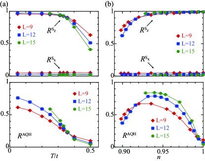
Figure 2: (a) Temperature dependence of correlation ratios for z-AFM and x-AFM orders (top panel) and AQH order (bottom panel) at doping $n=0.95$. Here, $L$ is the system size, $\lambda=0.1$ and $J_{z}=2$ in units of $t$. (b) Same as (a) for varying electron density $n$ at temperature $T=1/20$.

To verify the above low-energy theory, we measure equal-time correlation functions

$$C^{\alpha}(\mathbf{q})\equiv\frac{1}{L^{2}}\sum_{\mathbf{r},\mathbf{r}^{\prime}}\langle\hat{O}^{\alpha}_{\mathbf{r}}\hat{O}_{\mathbf{r}^{\prime}}^{\alpha}\rangle e^{i\mathbf{q}\cdot(\mathbf{r}-\mathbf{r}^{\prime})}$$ (7)

of fermion spin $\hat{O}_{\mathbf{r}}^{S_{z}(S_{xy})}=\hat{S}^{z(xy)}_{\mathbf{r},A}-\hat{S}^{z(xy)}_{\mathbf{r},B}$ with $\hat{S}^{\alpha}_{\mathbf{r}}=\frac{1}{2}\hat{c}^{\dagger}_{\mathbf{r}}\sigma^{\alpha}\hat{c}^{\phantom{\dagger}}_{\mathbf{r}}$, and the operator corresponding to the Haldane mass, $\hat{O}^{\text{AQH}}_{\boldsymbol{r}}=\sum_{\langle\langle\boldsymbol{\delta},\boldsymbol{\delta^{\prime}}\rangle\rangle,\sigma}e^{i\Phi_{\boldsymbol{r}+\boldsymbol{\delta},\boldsymbol{r}+\boldsymbol{\delta}^{\prime}}}\hat{c}^{\dagger}_{\boldsymbol{r}+\boldsymbol{\delta},\sigma}\hat{c}_{\boldsymbol{r}+\boldsymbol{\delta^{\prime}},\sigma}$. Here, $\boldsymbol{r}$ specifies a unit cell, or hexagon, and $\langle\langle\boldsymbol{\delta},\boldsymbol{\delta^{\prime}}\rangle\rangle$ runs over the next-nearest-neighbor sites of this hexagon. After computing the correlation functions, we extracted the renormalization-group invariant correlation ratios [24, 25]

$$R^{\alpha}=1-\frac{C^{\alpha}({\mathbf{q}_{0}}+\delta{\mathbf{q}})}{C^{\alpha}(\mathbf{q}_{0})}.$$ (8)

Here ${\mathbf{q}_{0}}$ is the ordering wave vector and ${\boldsymbol{q}}_{0}+\delta{\boldsymbol{q}}$ the longest wave-length fluctuation of the ordered state for a given lattice size. Long-range AFM and AQH orders here imply a divergence of the corresponding correlation functions $C^{\alpha}(\mathbf{q}_{0}=0)$. Accordingly, $R^{\alpha}\to 1$ for $L\to\infty$ in the ordered phase, whereas $R^{\alpha}\to 0$ in the disordered phase. At the critical point, $R^{\alpha}$ becomes scale-invariant for sufficiently large system size $L$, leading to a crossing of results for different $L$.

We find the altermagnetic phase in the range of parameters, specifically temperatures $T$ and electron densities $n$, shown in Fig. 2. Figure 2 (a) shows the results as a function of $T$ at $n=0.95$. The onset of the AFM in spin-$z$ ($x$) direction, termed $z$-AFM ($x$-AFM), is detected from the crossing of $R^{S_{z}}(R^{S_{x}})$, whereas the onset of the AQH order can be detected from $R^{\text{AQH}}$. As the temperature decreases, we observe the onset of the $z$-AFM order. We note that $z$-AFM only breaks time reversal symmetry such that ordering at finite temperature is allowed. A key feature is that its appearance coincides with the onset of the AQH order. Indeed, the data for $R^{\text{AQH}}$ are consistent with a finite-temperature phase transition to the $z$-AFM phase. Furthermore, within the range of parameters we investigated, we do not observe the emergence of the $x$-AFM order. Results as a function of $n$ for $T=1/20$ are presented in Fig 2(b). The consequence of the simultaneous emergence of both $z$-AFM and AQH orders persists against changes in electron density away from half filling. At half-filling the $z$-AFM ordering persists while AQH correlations are suppressed. This stands in agreement with our symmetry analysis that should the particle-hole symmetry forbids a linear coupling between the AQH and $z$-AFM orders in the Ginzburg-Landau functional.

AHE in mean field approximation.— Within a mean field approximation the AHE that emerges in the interacting modified Kane-Mele model can be accessed directly. Using the spin-dependent sublattice basis $\left(\psi_{A\uparrow},\psi_{B\uparrow},\psi_{A\downarrow},\psi_{B\downarrow}\right)$ it, the corresponding Hamiltonian, given by Eq. 2, reduces to

$$H^{\text{MF}}({\mathbf{k}})=(\epsilon-\mu)\sigma_{0}\tau_{0}+a_{\mathbf{k}}\tau_{0}\sigma_{z}+\mathbf{h}({\mathbf{k}},\sigma_{z})\cdot\boldsymbol{\tau},$$ (9)

where $h(\mathbf{k})=(b_{\mathbf{k}},c_{\mathbf{k}},h_{z})$, $h_{z}=-\Delta M^{\text{AFM}}_{z}\sigma_{z}$, $\Delta=\frac{3}{2}J_{z}+\frac{3}{4}|J_{z}|$, $\mu$ is the chemical potential, $\epsilon=\frac{3}{8}|J_{z}|(n-1)$, $n=n_{a}=n_{b}$ is the electron density of an atom A or B, with $n_{l}=\langle\hat{n}_{l\uparrow}\rangle+\langle\hat{n}_{l\downarrow}\rangle$, $l=a,\,b$ being the sublattice index. The antiferromagnetic $M^{\text{AFM}}_{z}$ order parameter along the $z$ direction is expressed in terms of the on-site magnetization as $M^{\text{AFM}}_{z}=\frac{1}{2}\left(m^{a}_{z}-m^{b}_{z}\right)$, where $m^{l}_{z}=\frac{1}{2}\left(\langle\hat{n}_{l\uparrow}\rangle-\langle\hat{n}_{l\downarrow}\rangle\right)$. The hopping terms $a_{\mathbf{k}}$, $b_{\mathbf{k}}$ and $c_{\mathbf{k}}$ are given by $a_{\mathbf{k}}=2\lambda\sum_{i=1}^{3}\sin\left(\mathbf{k}\cdot\mathbf{a}_{i}\right)$, $b_{\mathbf{k}}=t\sum_{i=1}^{3}\cos(\mathbf{k}\cdot\mathbf{\delta}_{i})$, $c_{\mathbf{k}}=t\sum_{i=1}^{3}\sin(\mathbf{k}\cdot\mathbf{\delta}_{i})$, $\mathbf{\delta}_{i}$ and $\mathbf{a}_{i}$ are, respectively, the vectors connecting NN and NNN sites; $\mathbf{a}_{1}=\sqrt{3}a(-\frac{1}{2},\frac{\sqrt{3}}{2})$, $\mathbf{a}_{2}=\sqrt{3}a(-\frac{1}{2},-\frac{{\sqrt{3}}}{2})$, $\mathbf{a}_{3}=\sqrt{3}a(1,0)$, $\mathbf{\delta}_{1}=a(\frac{\sqrt{3}}{2},\frac{1}{2})$, $\mathbf{\delta}_{2}=a(-\frac{\sqrt{3}}{2},\frac{1}{2})$, $\mathbf{\delta}_{3}=a(0,-1)$, where $a$ is the distance between NN sites. $\tau_{0}$ ($\sigma_{0}$) is the $2\times 2$ identity matrix in the sublattice (spin) space.

The energies of the mean field Hamiltonian (Eq. 9) are given by

$$E^{\text{MF}}_{\alpha,\sigma}({\mathbf{k}})=\epsilon-\mu+a_{\mathbf{k}}\sigma+\alpha\sqrt{b^{2}_{\mathbf{k}}+c^{2}_{\mathbf{k}}+\left(\Delta M^{\text{AFM}}_{z}\right)^{2}},$$

where $\alpha=\pm$ ($\sigma=\pm$) is the band (spin) index. The spin-dependent mass term $h_{z}$ in Eq. (9) breaks TRS and a non-vanishing Berry curvature (BC) is expected away from half-filling. For a given spin projection $\sigma$, the BC of a band $\alpha$ can be expressed as [26, 27]

$$\Omega^{\alpha}_{z}(\sigma,\mathbf{k})=-\frac{\alpha}{2|\mathbf{h}({\mathbf{k}})|^{3}}\mathbf{h}(\mathbf{k})\cdot\left[\partial_{k_{x}}\mathbf{h}(\mathbf{k})\times\partial_{k_{y}}\mathbf{h}(\mathbf{k})\right]$$

and the anomalous Hall (AH) conductivity [5] is given by the integral

$$\sigma_{\rm Hall}=-\frac{e^{2}}{\hbar}\frac{1}{(2\pi)^{2}}\sum_{\sigma,\alpha}\int_{BZ}d\mathbf{k}\;\Omega^{\alpha}_{z}(\sigma,\mathbf{k})f_{\alpha}(\mathbf{k},\mu),$$

$f_{\alpha}(\mathbf{k},\mu)$ being the Fermi-Dirac distribution function  [28]. $\sigma_{\rm Hall}$ can be computed using the values of the chemical potential and the AFM magnetization $M^{\text{AFM}}_{z}$ extracted from the mean field calculations. The results are depicted in Fig. 3 showing $\sigma_{\rm Hall}$ as function of the electronic density $n$.

The occurrence of a non-vanishing AH conductivity can be understood from the spin-valley dependence of the BC and the offset of the Dirac points induced by the modified Kane-Mele term $a_{\mathbf{k}}\sigma_{z}\tau_{0}$ (Eq. 9) which shifts oppositely the spin-split bands. To gain insights into these features, let us focus on the states $\mathbf{k}=\mu_{z}\mathbf{K}+\mathbf{q}$, ($\mathbf{q}\ll|\mathbf{K}|$) in the vicinity of the Dirac points $\mu_{z}\mathbf{K}$, where $\mu_{z}=\pm$ is the valley index. These states contribute mainly to the BC which reduces, around $\mu_{z}\mathbf{K}$, to

$$\Omega^{\alpha}_{z}(S_{z},\mathbf{q})=\operatorname{sgn}\frac{v_{F}\Delta M^{\text{AFM}}_{z}}{(\hbar v_{F}q)^{2}+\left(\Delta M^{\text{AFM}}_{z}\right)^{2}},$$ (10)

where $\operatorname{sgn}=-\alpha\mu_{z}\sigma$ is the sign of the BC and $\hbar v_{F}=\frac{3}{2}at$
Given the spin-dependent offset of the Dirac points, a spin-split sub-band $E^{\text{MF}}_{\alpha,\sigma}({\mathbf{k}})$ ($E^{\text{MF}}_{\alpha,-\sigma}({\mathbf{k}})$) of an occupied band $\alpha$, contributes to the BC by the states around the valley $\mu_{z}$ ($-\mu_{z}$), which results into a non-vanishing total BC, away from half filling.

The doping dependence of the AH conductivity (see Fig. 3) reflects the behavior of the secondary order parameter of Haldane type $N_{\rm AQH}$. At half-filling ($n=1$), $\sigma_{\rm Hall}$ vanishes as the bands below the Fermi level are fully occupied, resulting into a zero BC. By decreasing $n$ from half-filling, $\sigma_{\rm Hall}$ increases up to a maximum value, at a doping $n_{c}$, then it drops and vanishes below a critical doping value $n_{c0}$. The larger the coupling constant $J_{z}$, the smaller $n_{c0}$. For a fixed $J_{z}$, the increase of $\sigma_{\rm Hall}$ can be understood from the BC contribution which is enhanced as the area of the spin-polarized Fermi surface increases. The drop of $\sigma_{\rm Hall}$ is a consequence of the sharp decrease of $M^{\text{AFM}}_{z}$ below $n_{c}$, inducing a decrease of the BC The doping regime with a non-zero AH conductivity gets wider as $J_{z}$ increases, which results from the enhancement of the mass term $M^{\text{AFM}}_{z}$.

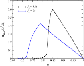
Figure 3: Anomalous Hall conductivity $\sigma_{\rm Hall}$ in units of $e^{2}/h$ as a function of the electron density $n$ for $J_{z}=1.6t$ and $J_{z}=2t$ using the mean field parameters for $n$ and $M^{\text{AFM}}_{z}$.

Conclusions and Outlook — We have shown how electronic interactions induce altermagnetism in a non-centrosymmetric system by stabilizing a primary AFM ordering that hosts a secondary one that directly induces the altermagnetic anomalous Hall effect. Specifically, our quantum Monte Carlo calculation on interacting modified Kane-Mele lattice model reveal a finite temperature phase transition into an altermagnetically ordered state, whose physical features are captured by its effective continuum theory. The interacting model may in principle be implemented in cold atoms in optical lattices which have been proposed to realize altermagnetism [29]. Interestingly, recently an experimental realization of a non-centrosymmetric 3D altermagnet has been reported in GdAlSi, a collinear antiferromagnetic Weyl semimetal [30]. This suggests generalization of the lattice model to higher dimensions to determine how electronic correlations generate Berry curvature in altermagnetic semi-metals that may as well harbor 3D electronic topology.