Probability vector representation of the Schrödinger equation
and noninvasive measurability for Leggett–Garg inequalities

Abstract

Leggett–Garg inequalities place bounds on the temporal correlations of a system based on the principles of macroscopic realism (MR) and noninvasive measurability (NM). Their conventional formulation relies on the ensemble-averaged products of observables measured at different instants of time. However, this expectation value based approach does not provide a clear definition of NM. A complete description that enables a precise understanding and captures all physically relevant features requires the study of probability distributions associated with noncommuting observables. In this article, we propose a scheme to describe the dynamics of generic $N$-level quantum systems via a probability vector representation of the Schrödinger equation and define a precise notion of NM for the probability distributions of noncommuting observables. This allows us to elucidate MR itself more clearly, eliminating any potential confusion. In addition, we introduce a measure to quantify violations of NM for arbitrary quantum states. For single-qubit systems, we pinpoint the pivotal relation that establishes a connection between the disturbance of observables incurred during a measurement and the resulting NM violation.

I Introduction

The distinction between classical and quantum phenomena has garnered considerable attention over the years. In contrast to the deterministic nature of classical mechanics, which accurately describes physical events on the macroscopic scales we experience in our day-to-day lives, quantum mechanics is fundamentally nondeterministic, and its precise role in the emergence of macroscopic phenomena is yet to be fully understood. To examine the breakdown of quantum coherence, Leggett and Garg devised an idealized experimental bound founded on the principles of macroscopic realism (MR) and noninvasive measurability (NM) [1]. MR posits that physical properties of macroscopic systems exist independent of our observation, i.e. measurements on macroscopic systems merely reveal stable preexisting values. In other words, the moon is there even if nobody looks [2]. In a trivial extension of quantum mechanics to large scales, macroscopic objects like Schrödinger’s cat are described by a superposition of distinct states, and MR is broken. A more general concept of realism within hidden variable theories encompasses MR as a subset. NM postulates that the measurement process has no bearing on the state of the system being measured, i.e. there is no backreaction of the measurement on the subsequent system dynamics.

Let us consider a non-quantum system $S$ which has a corresponding $N$-dimensional quantum system $S_{\text{QM}}$ that shares the same observables. Then, there exists a complete set of $N^{2}-1$ observables $\{Q,\bar{Q}_{1},\cdots,\bar{Q}_{N^{2}-2}\}$ for $S_{\text{QM}}$ that uniquely determine the quantum density operator $\hat{\rho}$ of $S_{\text{QM}}$ via quantum tomography. However, in quantum mechanics the operators associated with these observables do in general not commute. The observables are assumed to be observed in $S$, at least when they are measured at distinct points in time. In this article, NM measurements of an observable $Q$ of the system $S$ (not $S_{\text{QM}}$) are defined as measurements in which the probability distributions of all other observables $\bar{Q}_{n}$ remain unchanged while the initial probability distribution of $Q$ collapses into a more sharply peaked distribution. Such an NM measurement does not exist in quantum mechanics, but may be allowed in more general theories like hidden variable theories. We regard the collapse of the initial probability distribution of $Q$ as mere knowledge update about $Q$, not as disturbance against the fundamental degrees of freedom of $S$, including $Q$. This interpretation of updating information through measurement without causing a disturbance aligns with the standard approach for macroscopic objects in classical statistical mechanics.

Predicated on MR and NM, experimentally testable inequalities of the form derived in Ref. [1] (“Leggett–Garg inequalities”, abbrev. LGIs) bound the temporal correlations of a system in sequential measurements of observables. This is similar in spirit to the Bell [4] and CHSH inequalities [5], which place bounds on the correlations in measurements of spatially separated systems based on the principles of realism and locality. A naive extrapolation of quantum mechanics to the macroscopic regime violates both types of inequalities. Reciprocally, the dynamics of a system that violates either LGIs or Bell/CHSH-type inequalities cannot be understood within the framework of traditional classical mechanics [6, 7].

Various proposals amenable to experimental verification of LGIs have been explored, including but not limited to quasiprobabilistic approaches [8, 9, 10], continuous variable versions [11], and using expanded data sets obtained from finer-grained measurements [12]. Violations of LGIs have been confirmed in numerous experiments involving different physical systems and using different types of measurements [13, 14, 15, 16, 17] (see also Table 1 of Ref. [3]).

Nevertheless, the precise scale up to which we can detect the quantumness of macroscopic objects in experiments remains elusive. LGIs are one of the principal tools to investigate how quantum coherence in the form of superpositions and/or entanglement is lost in the macroscopic realm. In addition, the possibility of using LGIs to probe the quantumness of gravity through gravitationally induced violations has recently been put forward [10].

In certain LGIs, NM plays a more crucial role compared to MR. An example of this is found in the two-time LGIs for a single qubit. Let us consider a spin observable $Q=\pm 1$ for the qubit and perform measurements at $t_{1}$ and $t_{2}>t_{1}$, estimating the probability distribution $p(Q_{1}=Q(t_{1}),Q_{2}=Q(t_{2}))$. Here, we do not need to assume MR since the probability $p(Q_{1},Q_{2})$ is determined directly by the experiment. Then, the following inequality trivially holds:

$$\sum_{Q_{1}=\pm 1}\sum_{Q_{2}=\pm 1}(1+s_{1}Q_{1})(1+s_{2}Q_{2})p(Q_{1},Q_{2})\geqslant 0,$$ (1)

with $s_{1}=\pm 1$ and $s_{2}=\pm 1$. This inequality is rewritten as

$$1+s_{1}\langle Q_{1}\rangle+s_{2}\langle Q_{2}\rangle+s_{1}s_{2}\langle Q_{2}Q_{1}\rangle\geqslant 0,$$ (2)

where the bracket is defined such that $\langle f(Q_{1},Q_{2})\rangle\mathrel{\hbox to0.0pt{\raisebox{1.29167pt}{$\cdot$}\hss}\raisebox{-1.29167pt}{$\cdot$}}=\sum_{Q_{1},Q_{2}}f(Q_{1},Q_{2})p(Q_{1},Q_{2})$ for a function $f$ of $Q_{1}$ and $Q_{2}$. NM for the first measurement at $t=t_{1}$ implies $\langle Q_{2}\rangle=\langle Q_{2}\rangle_{\bar{1}}$, where

$$\langle Q_{2}\rangle_{\bar{1}}\mathrel{\hbox to0.0pt{\raisebox{1.29167pt}{$\cdot$}\hss}\raisebox{-1.29167pt}{$\cdot$}}=\!\!\sum_{Q_{2}=\pm 1}\!Q_{2}p_{\bar{1}}(Q_{2}),$$ (3)

and $p_{\bar{1}}(Q_{2})$ denotes the probability to observe $Q_{2}$ at $t=t_{2}$ without performing the measurement of $Q_{1}$ at $t=t_{1}$. This yields the two-time LGI [18, 9] given by

$$1+s_{1}\langle Q_{1}\rangle+s_{2}\langle Q_{2}\rangle_{\bar{1}}+s_{1}s_{2}\langle Q_{2}Q_{1}\rangle\geqslant 0.$$ (4)

The breakdown of the two-time LGI in Eq. (4) is caused by $\Delta Q_{2}\mathrel{\hbox to0.0pt{\raisebox{1.29167pt}{$\cdot$}\hss}\raisebox{-1.29167pt}{$\cdot$}}=\langle Q_{2}\rangle-\langle Q_{2}\rangle_{\bar{1}}\neq 0$ in experiments. If the first measurement at $t=t_{1}$ does not affect the second measurement at $t=t_{2}$, we obtain $\Delta Q_{2}=0$ as an NM result. In this case, the constraint $\Delta Q_{2}=0$ required for NM is more stringent than the bound set by the two-time LGI in Eq. (4), since the LGI can still hold even when $\Delta Q_{2}\neq 0$.

It is worth noting that the hidden variable theory for a single qubit proposed by J. S. Bell [4] precisely reproduces the same results of quantum mechanics by breaking NM. In his theory, all expectation values $\langle\sigma_{a}\rangle_{\text{HV}}$ of the spin component $\sigma_{a}$ with $a\in\{x,y,z\}$ are allowed as long as $\langle\sigma_{x}\rangle^{2}_{\text{HV}}+\langle\sigma_{y}\rangle^{2}_{\text{HV}}+\langle\sigma_{z}\rangle^{2}_{\text{HV}}\leqslant 1$ holds. Then, it is possible to define density matrices via the following tomography relation:

$$\hat{\rho}_{\text{HV}}\mathrel{\hbox to0.0pt{\raisebox{1.29167pt}{$\cdot$}\hss}\raisebox{-1.29167pt}{$\cdot$}}=\frac{1}{2}\left(\hat{I}+\langle\sigma_{x}\rangle_{\text{HV}}\hat{\sigma}_{x}+\langle\sigma_{y}\rangle_{\text{HV}}\hat{\sigma}_{y}+\langle\sigma_{z}\rangle_{\text{HV}}\hat{\sigma}_{z}\right),$$ (5)

where $\hat{I}$ denotes the two-dimensional identy matrix and $\hat{\sigma}_{a}$ are the Pauli matrices. Among the states described by $\hat{\rho}_{\text{HV}}$, there exist pure states denoted by $|\psi_{\text{HV}}\rangle\langle\psi_{\text{HV}}|$, which also appear in quantum mechanics. Similarly, all pure states in quantum mechanics are shared in Bell’s theory. Therefore, the “quantum coherence” of $|\psi_{\text{HV}}\rangle$ is reproduced by a superposition of two distinct states $|\pm_{\text{HV}}\rangle$ via $|\psi_{\text{HV}}\rangle=c_{+}|+_{\text{HV}}\rangle+c_{-}|-_{\text{HV}}\rangle$ with complex coefficients $c_{\pm}$, even though this is a hidden variable theory. In this realism (not MR) theory, the LGI for the single qubit in Eq. (4) is not satisfied in the same manner as in quantum mechanics, since the unavoidable backreaction of measurements leads to $\Delta Q_{2}\neq 0$.

In previous studies of LGIs, arguments related to NM have relied solely on the expectation values and ensemble averages of temporal correlations of observables. However, these quantities are secondary objects, derived from the probability distributions of observables in actual experiments. To provide a clearer and more fundamental definition of NM, we introduce a probability vector representation of the Schrödinger equation in this article. The concept of NM is unambiguously defined using the probability distributions in this representation. Based on this formalism, we precisely quantify the distinction between quantum mechanics and other theories in which NM holds. This ultimately allows us to better understand how fundamental differences between quantum mechanics and NM-compatible theories arise.

The remainder of this article is organized as follows: In Sec. II, we review mathematical preliminaries and derive the probability vector representation of the Schrödinger equation [Eq. (25)] which describes the evolution of a quantum system in terms of the probability distributions associated with its observables. In Sec. III, we highlight important differences between classical [Subsec. III.A] and quantum [Subsec. III.B] dynamics based on the description of a single-qubit system and introduce measures to quantify the violation of NM [Eq. (205)] caused by the backreaction of a measurement [Eq. (213)] and their interrelation [Eq. (218)]. The generalization to generic $N$-level systems is covered in Sec. IV. In Sec. V, we outline how the classification of quantum states as either NM-conforming or NM-violating could be performed by a machine learning algorithm in the case of very large $N$ (where a manual evaluation becomes infeasible in practice) and present a minimalistic proof-of-principle implementation. Lastly, we summarize our results and discuss their physical implications (Sec. VI).

II Probability vector Representation
      of the Schrödinger Equation

Our objective in this section is to derive a probability vector representation for quantum dynamics that is suitable for investigating violations of NM. The Schrödinger equation for an $N$-level system represented by the quantum state $\hat{\rho}(t)$ at time $t$ is given by

$$i\hbar\frac{d}{dt}\hat{\rho}(t)=\left[\hat{H},\hat{\rho}(t)\right],$$ (6)

where $\big{[}\hat{A},\hat{B}\big{]}\mathrel{\hbox to0.0pt{\raisebox{1.29167pt}{$\cdot$}\hss}\raisebox{-1.29167pt}{$\cdot$}}=\hat{A}\hat{B}-\hat{B}\hat{A}$ denotes the commutator of two operators $\hat{A}$ and $\hat{B}$. The generators $\hat{\lambda}_{n}$ of $\mathrm{SU(N)}$ satisfy

$$\hat{\lambda}_{n}^{{\dagger}}=\hat{\lambda}_{n},\quad\operatorname{Tr}\left[\hat{\lambda}_{n}\right]=0,\quad\operatorname{Tr}\left[\hat{\lambda}_{n}\hat{\lambda}_{n^{\prime}}\right]=N\delta_{nn^{\prime}},$$ (7)

where $n,n^{\prime}\in\{1,\dots,\mathrm{dim[SU(N)]}\}$ with $\mathrm{dim[SU(N)]}=N^{2}-1$. The corresponding Lie algebra is given by

$$\left[\hat{\lambda}_{n},\hat{\lambda}_{n^{\prime}}\right]=i\sum_{n^{\prime\prime}=1}^{N^{2}-1}\gamma_{nn^{\prime}}^{n^{\prime\prime}}\hat{\lambda}_{n^{\prime\prime}},$$ (8)

where $\gamma_{nn^{\prime}}^{n^{\prime\prime}}$ labels real-valued coefficients. Any $N$-level quantum state is decomposable in terms of the $\mathrm{SU(N)}$ generators $\hat{\lambda}_{n}$ via the so-called Bloch representation

$$\hat{\rho}(t)=\frac{1}{N}\left(\hat{I}+\sum_{n=1}^{N^{2}-1}\left\langle\lambda_{n}(t)\right\rangle\hat{\lambda}_{n}\right),$$ (9)

where $\hat{I}$ denotes the $N$-dimensional identity matrix, and the expectation values of the $\mathrm{SU(N)}$ generators are given by

$$\left\langle\lambda_{n}(t)\right\rangle=\operatorname{Tr}\left[\hat{\lambda}_{n}\hat{\rho}(t)\right].$$ (10)

Their time derivatives are computed as

$$\frac{d}{dt}\left\langle\lambda_{n}(t)\right\rangle =\operatorname{Tr}\left[\hat{\lambda}_{n}\frac{d}{dt}\hat{\rho}(t)\right]=\frac{1}{i\hbar}\operatorname{Tr}\left[\hat{\lambda}_{n}\left[\hat{H},\hat{\rho}(t)\right]\right]$$

$$=\frac{1}{i\hbar}\operatorname{Tr}\left[\hat{\rho}(t)\left[\hat{\lambda}_{n},\hat{H}\right]\right].$$ (11)

It is useful to introduce the real-valued coefficients

$$h_{nn^{\prime}} \mathrel{\hbox to0.0pt{\raisebox{1.29167pt}{$\cdot$}\hss}\raisebox{-1.29167pt}{$\cdot$}}=-\frac{i}{N}\operatorname{Tr}\left[\hat{\lambda}_{n^{\prime}}\left[\hat{\lambda}_{n},\hat{H}\right]\right]=\frac{i}{N}\operatorname{Tr}\left[\hat{H}\left[\hat{\lambda}_{n},\hat{\lambda}_{n^{\prime}}\right]\right]$$

$$=-\frac{1}{N}\sum_{n^{\prime\prime}=1}^{N^{2}-1}\gamma_{nn^{\prime}}^{n^{\prime\prime}}\operatorname{Tr}\left[\hat{H}\hat{\lambda}_{n^{\prime\prime}}\right].$$ (12)

One can then show that

$$\left[\hat{\lambda}_{n},\hat{H}\right]=i\sum_{n^{\prime}=1}^{N^{2}-1}h_{nn^{\prime}}\hat{\lambda}_{n^{\prime}}.$$ (13)

The Schrödinger equation in the form of Eq. (6) can thus be recast in terms of the expectation values $\left\langle\lambda_{n}(t)\right\rangle$ as follows:

$$\frac{d}{dt}\left\langle\lambda_{n}(t)\right\rangle=\frac{1}{\hbar}\sum_{n^{\prime}=1}^{N^{2}-1}h_{nn^{\prime}}\left\langle\lambda_{n^{\prime}}(t)\right\rangle.$$ (14)

This is a generalization of the standard Bloch equation for a single qubit [$N=2$] to arbitrary $N$. The spectral decomposition of the $\mathrm{SU(N)}$ generators $\hat{\lambda}_{n}$ is given by

$$\hat{\lambda}_{n}=\sum_{k=1}^{N}\lambda_{n}(k)\hat{P}_{n}(k),$$ (15)

where $\lambda_{n}(k)$ denote their eigenvalues and $\hat{P}_{n}(k)$ their projectors, respectively. The emergent probability of $\lambda_{n}(k)$ for the observable $\hat{\lambda}_{n}$ in the state $\hat{\rho}(t)$ is

$$p_{n}(k,t)=\operatorname{Tr}\left[\hat{P}_{n}(k)\hat{\rho}(t)\right]$$ (16)

and satisfies the normalization condition

$$\sum\limits_{k=1}^{N}p_{n}(k,t)=1.$$ (17)

The expectation values can be expressed in terms of their respective emergent probabilities, i.e.

$$\left\langle\lambda_{n}(t)\right\rangle=\sum\limits_{k=1}^{N}\lambda_{n}(k)p_{n}(k,t),$$ (18)

and their time derivatives are computed using

$$\frac{d}{dt}p_{n}(k,t) =\operatorname{Tr}\left[\hat{P}_{n}(k)\frac{d}{dt}\hat{\rho}(t)\right]=\frac{1}{i\hbar}\operatorname{Tr}\left[\hat{P}_{n}(k)\left[\hat{H},\hat{\rho}(t)\right]\right]$$

$$=\frac{1}{i\hbar}\operatorname{Tr}\left[\hat{\rho}(t)\left[\hat{P}_{n}(k),\hat{H}\right]\right].$$ (19)

Expanding the right-hand side of this equation with respect to the generators $\hat{\lambda}_{n}$ yields

$$\frac{1}{i\hbar}\left[\hat{P}_{n}(k),\hat{H}\right]=\sum\limits_{n^{\prime}=1}^{N^{2}-1}K_{nn^{\prime}}(k)\hat{\lambda}_{n^{\prime}},$$ (20)

with coefficients $K_{nn^{\prime}}(k)$ given by

$$K_{nn^{\prime}}(k)=\frac{1}{Ni\hbar}\operatorname{Tr}\left[\hat{\lambda}_{n^{\prime}}\left[\hat{P}_{n}(k),\hat{H}\right]\right].$$ (21)

Substituting the spectral decomposition of $\hat{\lambda}_{n^{\prime}}$ [cf. Eq. (15)] into Eq. (20), we obtain

$$\frac{1}{i\hbar}\left[\hat{P}_{n}(k),\hat{H}\right]=\sum_{n^{\prime}=1}^{N^{2}-1}\sum_{k^{\prime}=1}^{N}K_{nn^{\prime}}(k)\lambda_{n^{\prime}}(k^{\prime})\hat{P}_{n^{\prime}}(k^{\prime}).$$ (22)

Defining the coefficients

$$H_{nn^{\prime}}(k,k^{\prime}) \mathrel{\hbox to0.0pt{\raisebox{1.29167pt}{$\cdot$}\hss}\raisebox{-1.29167pt}{$\cdot$}}=\frac{\lambda_{n^{\prime}}(k^{\prime})}{Ni\hbar}\operatorname{Tr}\left[\hat{\lambda}_{n^{\prime}}\left[\hat{P}_{n}(k),\hat{H}\right]\right],$$ (23)

the following relation holds:

$$\frac{1}{i\hbar}\left[\hat{P}_{n}(k),\hat{H}\right]=\sum_{n^{\prime}=1}^{N^{2}-1}\sum_{k=1}^{N}H_{nn^{\prime}}(k,k^{\prime})\hat{P}_{n^{\prime}}(k^{\prime}).$$ (24)

Substitution of Eq. (24) into Eq. (19) reveals that the Schrödinger equation [cf. Eq. (6)] can be rewritten in the probability vector form [i.e. expressed in terms of the emergent probabilities $p_{n}(k,t)$] as follows:

$$\frac{d}{dt}p_{n}(k,t)=\sum_{n^{\prime}=1}^{N^{2}-1}\sum_{k^{\prime}=1}^{N}H_{nn^{\prime}}(k,k^{\prime})p_{n^{\prime}}(k^{\prime},t).$$ (25)

This formulation can be straightforwardly extended to the case of open quantum systems by considering the Lindblad master equation. The initial condition of Eq. (25) is chosen such that the underlying probability distribution describes a valid quantum state. Therefore, $p_{n}(k,0)=\operatorname{Tr}\big{[}\hat{P}_{n}(k)\hat{\rho}(0)\big{]}$ holds for an initial state described by the density matrix $\hat{\rho}(0)$. Using Eqs. (23), (25), and the fact that $\sum_{k=1}^{N}\hat{P}_{n}(k)=\hat{I}$, it is straightforward to show that

$$\frac{d}{dt}\sum_{k=1}^{N}p_{n}(k,t)=0,$$ (26)

and thus the normalization condition Eq. (17) holds at any time $t$:

$$\sum_{k=1}^{N}p_{n}(k,t)=\sum_{k=1}^{N}p_{n}(k)=1,$$ (27)

where $p_{n}(k)\equiv p_{n}(k,0)$. Let $\vec{p}(t)$ represent the $N(N^{2}-1)$-dimensional probability vector

$$\vec{p}(t)=\left[\begin{array}[c]{c}p_{1}(1,t)\\ \vdots\\ p_{1}(N,t)\\ \vdots\\ p_{N^{2}-1}(1,t)\\ \vdots\\ p_{N^{2}-1}(N,t)\end{array}\right].$$ (35)

Using the $N(N^{2}-1)\times N(N^{2}-1)$ matrix $H=\left[H_{nn^{\prime}}(k,k^{\prime})\right]$ whose elements are prescribed by Eq. (23), the solution of Eq. (25) is obtained as

$$\left[\begin{array}[c]{c}p_{1}(1,t)\\ \vdots\\ p_{1}(N,t)\\ \vdots\\ p_{N^{2}-1}(1,t)\\ \vdots\\ p_{N^{2}-1}(N,t)\end{array}\right]=\exp\left(tH\right)\left[\begin{array}[c]{c}p_{1}(1)\\ \vdots\\ p_{1}(N)\\ \vdots\\ p_{N^{2}-1}(1)\\ \vdots\\ p_{N^{2}-1}(N)\end{array}\right],$$ (50)

which can be rewritten in the series expansion form

$$\left[\begin{array}[c]{c}p_{1}(1,t)\\ \vdots\\ p_{1}(N,t)\\ \vdots\\ p_{N^{2}-1}(1,t)\\ \vdots\\ p_{N^{2}-1}(N,t)\end{array}\right]=\sum_{n=0}^{\infty}\frac{t^{n}}{n!}H^{n}\left[\begin{array}[c]{c}p_{1}(1)\\ \vdots\\ p_{1}(N)\\ \vdots\\ p_{N^{2}-1}(1)\\ \vdots\\ p_{N^{2}-1}(N)\end{array}\right].$$ (65)

The numerical computation of $H^{n}$ does not require the exact diagonalization of $H$ and only takes a brief amount of time. Consequently, the right-hand side of Eq. (65) can be calculated without facing significant obstacles even for sizable values of $N$.

For an NM measurement of $\hat{\lambda}_{n}$ at time $t=0$, the expectation values $\left\langle\lambda_{n}\right\rangle$ of $\hat{\lambda}_{n}$ are determined by [cf. Eq. (18)]

$$\left\langle\lambda_{n}\right\rangle=\sum_{k=1}^{N}\lambda_{n}(k)p_{n}(k).$$ (66)

If an NM measurement of $\hat{\lambda}_{1}$ is performed and the result $\lambda_{1}(1)$ is obtained, the $\lambda_{1}$ sector of the probability vector $\vec{p}$ induces a collapse of the state vector such that $p^{\prime}_{1}(k)_{1,1}=\delta_{k1}$, while the other sectors remain unaffected:

(100)

This provides a precise definition of NM for the probability distribution. Analogously, one can define probability distributions $p^{\prime}_{n^{\prime}}(k^{\prime})_{n,k}$ after an NM measurement of $\hat{\lambda}_{n}$ at time $t=0$ results in the observation of the eigenvalue $\lambda_{n}(k)$. The $\lambda_{n}$ sector of $\vec{p}$ induces a collapse of the state vector, while the other sectors remain unaffected:

$$p^{\prime}_{n^{\prime}}(k^{\prime})_{n,k}=\delta_{n^{\prime}n}\delta_{k^{\prime}k}+\left(1-\delta_{n^{\prime}n}\right)p_{n^{\prime}}(k^{\prime}).$$ (101)

However, it is not assured that the post-measurement probability vector $\vec{p}\mkern 2.0mu\vphantom{p}^{\prime}_{n,k}=[p^{\prime}_{n^{\prime}}(k^{\prime})_{n,k}]$ always represents a valid quantum state. The expectation values of $\hat{\lambda}_{n^{\prime}}$ are evaluated as

$$\left\langle\lambda_{n^{\prime}}\right\rangle^{\prime}_{n,k}=\sum_{k^{\prime}=1}^{N}\lambda_{n^{\prime}}(k^{\prime})p^{\prime}_{n^{\prime}}(k^{\prime})_{n,k}.$$ (102)

The post-measurement density matrix is given by

$$\hat{\rho}^{\prime}_{n,k}=\frac{1}{N}\left(\hat{I}+\sum_{n^{\prime}=1}^{N^{2}-1}\left\langle\lambda_{n^{\prime}}\right\rangle^{\prime}_{n,k}\hat{\lambda}_{n^{\prime}}\right)$$ (103)

and could possess negative eigenvalues, which would imply that the corresponding operator is no longer positive semidefinite (which, in a slight abuse of notation, may be denoted by $\hat{\rho}^{\prime}_{n,k}\ngeqslant 0$). In this sense, the presence of negative eigenvalues signifies the violation of NM.

Next, for an arbitary initial state $\hat{\rho}(0)$, let us introduce a measure $\gamma_{n,k}$ that quantifies the NM violation when a measurement of $\hat{\lambda}_{n}$ observes $\lambda_{n}(k)$. To this end, we first evaluate $p_{n^{\prime}}(k^{\prime})$ via $\operatorname{Tr}\big{[}\hat{P}_{n^{\prime}}(k^{\prime})\hat{\rho}(0)\big{]}$ [cf. Eq. (16)]. After the measurement, its $\lambda_{n}$ sector undergoes the following transition:

$$p_{n}(k^{\prime})\;\Rightarrow\;p^{\prime}_{n}(k^{\prime})=\delta_{k^{\prime}k}.$$ (104)

Then, the expectation value of $\hat{\lambda}_{n}$ is computed as

$$\left\langle\lambda_{n}\right\rangle^{\prime}_{n,k}=\sum_{k^{\prime}=1}^{N}\lambda_{n^{\prime}}(k^{\prime})p^{\prime}_{n}(k^{\prime})=\lambda_{n}(k).$$ (105)

For sectors $n^{\prime}\neq n$ on the other hand, the probabilities remain unchanged,

$$p_{n^{\prime}}(k)\;\Rightarrow\;p^{\prime}_{n^{\prime}}(k^{\prime})=p_{n^{\prime}}(k^{\prime}),$$ (106)

and the expectation value of $\hat{\lambda}_{n^{\prime}\neq n}$ is given by

$$\left\langle\lambda_{n^{\prime}}\right\rangle^{\prime}_{n,k}\equiv\left\langle\lambda_{n^{\prime}}\right\rangle=\operatorname{Tr}\left[\hat{\lambda}_{n^{\prime}}\hat{\rho}(0)\right].$$ (107)

For $\hat{\rho}(0)$ the pseudo-density matrix after the measurement can be defined as

$$\hat{\rho}^{\prime}_{n,k}=\frac{1}{N}\left(\hat{I}+\sum_{n^{\prime}=1}^{N^{2}-1}\left\langle\lambda_{n^{\prime}}\right\rangle^{\prime}_{n.k}\hat{\lambda}_{n^{\prime}}\right).$$ (108)

More specifically, it can be expressed as

$$\hat{\rho}^{\prime}_{n,k}=\frac{1}{N}\left(\hat{I}+\lambda_{n}(k)\hat{\lambda}_{n}+\sum_{n^{\prime}\neq n}\operatorname{Tr}\left[\hat{\lambda}_{n^{\prime}}\hat{\rho}(0)\right]\hat{\lambda}_{n^{\prime}}\right).$$ (109)

Let $p^{\prime}_{m}(n,k)$ label the eigenvalues in the spectral decomposition of $\hat{\rho}^{\prime}_{n,k}$, i.e.

$$\hat{\rho}^{\prime}_{n,k}=\sum_{m=1}^{N}p^{\prime}_{m}(n,k)\hat{P}^{\prime}_{m}(n,k).$$ (110)

The NM violation measure $\gamma(n,k)$ for $\hat{\rho}(0)$ is then defined as the sum of the absolute values of all negative eigenvalues:

$$\gamma_{n,k}\mathrel{\hbox to0.0pt{\raisebox{1.29167pt}{$\cdot$}\hss}\raisebox{-1.29167pt}{$\cdot$}}=\sum_{p^{\prime}_{m}(n,k)<0}\big{|}p^{\prime}_{m}(n,k)\big{|}.$$ (111)

The conclusion of this section warrants the following final remark: one can certainly verify the violation of NM by numerically diagonalizing $\hat{\rho}^{\prime}_{n,k}$, identifying the negative eigenvalues in its spectrum, and then confirming that $\gamma_{n,k}>0$. However, executing such a numerical diagonalization for large $N$ is a notably huge task that requires a significant amount of computational resources compared to the computation of $H^{n}$. Therefore, Eq. (65) provides a much more efficient way of investigating NM violations in large-$N$ systems. Some of the $p_{n^{\prime}}(k^{\prime},t)$ values in Eq. (65) can become negative at specific instances $t$ by taking $p_{n^{\prime}}(k^{\prime})=\operatorname{Tr}\big{[}\hat{P}_{n^{\prime}}(k^{\prime})\hat{\rho}^{\prime}_{n,k}\big{]}$ and an adequate Hamiltonian $\hat{H}$. By solving this equation, one can identify the presence of negative components within $p_{n^{\prime}}(k^{\prime},t)$, which serves as an indicator of the NM violation for $\hat{\rho}(0)$ in the large-$N$ case.

III Single-Qubit Systems

To account for the backreaction of quantum measurements on the probability distributions of observables for a single-qubit system, we first revisit the Bloch representation of quantum states. For a single qubit [$N=2$], the quantum state $\hat{\rho}$ is precisely specified by the expectation values $\langle\sigma_{x}\rangle$, $\langle\sigma_{y}\rangle$, $\langle\sigma_{z}\rangle$ of the three Pauli operators $\hat{\sigma}_{x}$, $\hat{\sigma}_{y}$, $\hat{\sigma}_{z}$ via

$$\hat{\rho}=\frac{1}{2}\left(\hat{I}+\langle\sigma_{x}\rangle\hat{\sigma}_{x}+\langle\sigma_{y}\rangle\hat{\sigma}_{y}+\langle\sigma_{z}\rangle\hat{\sigma}_{z}\right).$$ (112)

The state space is represented by a Bloch sphere (see Fig. 1), which is defined by the inequality

$$\langle\sigma_{x}\rangle^{2}+\langle\sigma_{y}\rangle^{2}+\langle\sigma_{z}\rangle^{2}\leqslant 1.$$ (113)

This condition guarantees that all eigenvalues of $\hat{\rho}$ remain nonnegative, which is commonly (again, in a slight abuse of notation) denoted as $\hat{\rho}\geqslant 0$. The emergent probabilities of the measurement outcomes $\pm 1$ for $\hat{\sigma}_{a}$ with $a\in\{x,y,z\}$ are computed as

$$p_{a}\left(\pm 1\right)=\operatorname{Tr}\left[\hat{P}_{a}(\pm 1)\hat{\rho}\right],$$ (114)

where the projection operator $\hat{P}_{a}(\pm 1)$ for $\hat{\sigma}_{a}$ is represented by $\hat{P}_{a}(\pm 1)\mathrel{\hbox to0.0pt{\raisebox{1.29167pt}{$\cdot$}\hss}\raisebox{-1.29167pt}{$\cdot$}}=\frac{1}{2}\big{(}\hat{I}\pm\hat{\sigma}_{a}\big{)}$. The Bloch sphere inequality of Eq. (113) can be rewritten in terms of the emergent probabilities as

$$\begin{aligned} &\big{(}p_{x}(+1)-p_{x}(-1)\big{)}^{2}+\big{(}p_{y}(+1)-p_{y}(-1)\big{)}^{2}\\ &\hskip 39.83385pt+\big{(}p_{z}(+1)-p_{z}(-1)\big{)}^{2}\leqslant 1.\end{aligned}$$ (115)

To examine violations of NM for a single-qubit system described by $\hat{\rho}$, it is convenient to consider the six-dimensional [in general $N(N^{2}-1)$-dimensional] real vector of emergent probabilities given by

$$\vec{p}=\left[\begin{array}[c]{c}p_{x}(+1)\\ p_{x}(-1)\\ p_{y}(+1)\\ p_{y}(-1)\\ p_{z}(+1)\\ p_{z}(-1)\end{array}\right].$$ (122)

The generic form of the time-independent Hamiltonian for a single qubit is given up to a constant by

$$\hat{H}=\frac{\hbar}{2}\left(B_{x}\hat{\sigma}_{x}+B_{y}\hat{\sigma}_{y}+B_{z}\hat{\sigma}_{z}\right),$$ (123)

where $B_{a}$ with $a\in\{x,y,z\}$ denote real parameters. In this case, the Schrödinger equation [cf. Eq. (6)] can be expressed through the ordinary Bloch equation [cf. Eq. (14)] as

$$\frac{d}{dt}\left[\begin{array}[c]{c}\langle\sigma_{x}(t)\rangle\\ \langle\sigma_{y}(t)\rangle\\ \langle\sigma_{z}(t)\rangle\end{array}\right]=\left[\begin{array}[c]{ccc}0&B_{z}&-B_{y}\\ -B_{z}&0&B_{x}\\ B_{y}&-B_{x}&0\end{array}\right]\left[\begin{array}[c]{c}\langle\sigma_{x}(t)\rangle\\ \langle\sigma_{y}(t)\rangle\\ \langle\sigma_{z}(t)\rangle\end{array}\right].$$ (133)

Before delving into the quantum probability vector representation, it is prudent to first revisit the analogous classical theory to ensure a comprehensive understanding of why the NM postulate is always satisfied by classical dynamics.

III.A Classical Dynamics

The classical equation of motion of a spin vector $\vec{S}=\big{[}S_{x}(t),S_{y}(t),S_{z}(t)\big{]}$ is given by

$$\frac{d}{dt}\left[\begin{array}[c]{c}S_{x}(t)\\ S_{y}(t)\\ S_{z}(t)\end{array}\right]=\left[\begin{array}[c]{ccc}0&B_{z}&-B_{y}\\ -B_{z}&0&B_{x}\\ B_{y}&-B_{x}&0\end{array}\right]\left[\begin{array}[c]{c}S_{x}(t)\\ S_{y}(t)\\ S_{z}(t)\end{array}\right],$$ (143)

where the initial condition is specified through the continuous real parameters $S_{0a}$ $\big{[}a\in\{x,y,z\}\big{]}$ as

$$\left[\begin{array}[c]{c}S_{x}(0)\\ S_{y}(0)\\ S_{z}(0)\end{array}\right]=\left[\begin{array}[c]{c}S_{0x}\\ S_{0y}\\ S_{0z}\end{array}\right].$$ (150)

In the following discussion, let the spin vector with its initial conditions be denoted by

$$\left[\begin{array}[c]{c}S_{x}(t)\\ S_{y}(t)\\ S_{z}(t)\end{array}\right]=\left[\begin{array}[c]{c}S_{x}(S_{0x},S_{0y},S_{0z},t)\\ S_{y}(S_{0x},S_{0y},S_{0z},t)\\ S_{z}(S_{0x},S_{0y},S_{0z},t)\end{array}\right].$$ (157)

Let $\rho_{0}\left(S_{0x},S_{0y},S_{0z}\right)$ be the classical probability distribution of the initial spin satisfying

$$\rho_{0}\left(S_{0x},S_{0y},S_{0z}\right)\geqslant 0,$$ (158)

and

$$\int\int\int\rho_{0}\left(S_{0x},S_{0y},S_{0z}\right)dS_{0x}dS_{0y}dS_{0z}=1.$$ (159)

The distribution $\rho\left(S_{x},S_{y},S_{z},t\right)$ at time $t$ is determined by

$$\begin{aligned} \rho\left(S_{x},S_{y},S_{z},t\right)&=\int\int\int\delta\big{(}S_{x}-S_{x}(S_{0x},S_{0y},S_{0z},t)\big{)}\delta\big{(}S_{y}-S_{y}(S_{0x},S_{0y},S_{0z},t)\big{)}\delta\big{(}S_{z}-S_{z}(S_{0x},S_{0y},S_{0z},t)\big{)}\\ &\hskip 189.21082pt\times\rho_{0}\left(S_{0x},S_{0y},S_{0z}\right)dS_{0x}dS_{0y}dS_{0z},\end{aligned}$$ (160)

and satisfies the equation of motion

$$\frac{\partial}{\partial t}\rho\left(S_{x},S_{y},S_{z},t\right)=-\left(S_{x},S_{y},S_{z}\right)\left[\begin{array}[c]{ccc}0&B_{z}&-B_{y}\\ -B_{z}&0&B_{x}\\ B_{y}&-B_{x}&0\end{array}\right]\left[\begin{array}[c]{c}\frac{\partial}{\partial S_{x}}\\ \frac{\partial}{\partial S_{y}}\\ \frac{\partial}{\partial S_{z}}\end{array}\right]\rho\left(S_{x},S_{y},S_{z},t\right).$$ (167)

Consider a measurement of $S_{a}$ $\big{[}a\in\{x,y,z\}\big{]}$ resulting in the observed spin $s=\pm 1$ of $S_{a}$ at $t=0$. The probability of $s$ for $S_{a}$ is computed via

$$\bar{p}_{a,s}=\int\int\int\Theta\left(sS_{0a}\right)\rho_{0}\left(S_{0x},S_{0y},S_{0z}\right)dS_{0x}dS_{0y}dS_{0z},$$ (168)

where $\Theta(x)$ denotes the Heaviside step function

$$\Theta(x)\mathrel{\hbox to0.0pt{\raisebox{1.29167pt}{$\cdot$}\hss}\raisebox{-1.29167pt}{$\cdot$}}=\begin{cases}\;1\quad\;\;x\geqslant 0\\ \;0\quad\;\;x<0\end{cases}.$$ (169)

The probability distribution subsequent to the measurement at $t=0$ is described by

$$\rho_{a,s}\left(S_{0x},S_{0y},S_{0z}\right)=\frac{\Theta\left(sS_{0a}\right)}{\bar{p}_{a,s}}\rho_{0}\left(S_{0x},S_{0y},S_{0z}\right).$$ (170)

From Eqs. (167) and (170), one can immediately ascertain that no backreaction from the measurement influences the

expectation value of any observable at a future time $t$. Since the relation

$$\begin{aligned} \rho\left(S_{x},S_{y},S_{z},t\right)&=\bar{p}_{a,+1}\rho_{a,+1}\left(S_{x},S_{y},S_{z},t\right)\\ &\hskip 22.19315pt+\bar{p}_{a,-1}\rho_{a,-1}\left(S_{x},S_{y},S_{z},t\right)\end{aligned}$$ (171)

is satisfied at time $t$, the expectation value

(172)

of a physical observable $O(S_{x},S_{y},S_{z})$ at time $t$ with measurement matches the expectation value $\int\int\int O(S_{x},S_{y},S_{z})\rho(S_{x},S_{y},S_{z},t)dS_{x}dS_{y}dS_{z}$ of that same observable without the measurement. This ensures the stability and predictability of the system even after measurements have been performed, thereby underscoring the classical nature of the described dynamics. Therefore, classical statistical mechanics is an example of an NM-compatible theory.

III.B Quantum Dynamics

To consider measurements and violations of NM in quantum dynamical systems, we introduce the six-dimensional probability vector $\vec{p}_{cl}$ as a comparison measure for the above-described classical theory by defining the discrete spin variables $\sigma_{a}=\pm 1$ as

$$\sigma_{x} =\epsilon\left(S_{x}\right)=\Theta\left(S_{x}\right)-\Theta\left(-S_{x}\right),$$ (173)

$$\sigma_{y} =\epsilon\left(S_{y}\right)=\Theta\left(S_{y}\right)-\Theta\left(-S_{y}\right),$$ (174)

$$\sigma_{z} =\epsilon\left(S_{z}\right)=\Theta\left(S_{z}\right)-\Theta\left(-S_{z}\right).$$ (175)

The classical probability vector $\vec{p}_{\mathrm{cl}}(t)$ at time $t$ is then given by [cf. Eq. (122)]

$$\vec{p}_{\mathrm{cl}}(t)=\left[\begin{array}[c]{c}\bar{p}_{x}(+1,t)\\ \bar{p}_{x}(-1,t)\\ \bar{p}_{y}(+1,t)\\ \bar{p}_{y}(-1,t)\\ \bar{p}_{z}(+1,t)\\ \bar{p}_{z}(-1,t)\end{array}\right]=\left[\begin{array}[c]{c}\sum_{\sigma_{y},\sigma_{z}}p_{\mathrm{cl}}(+1,\sigma_{y},\sigma_{z},t)\\ \sum_{\sigma_{y},\sigma_{z}}p_{\mathrm{cl}}(-1,\sigma_{y},\sigma_{z},t)\\ \sum_{\sigma_{x},\sigma_{z}}p_{\mathrm{cl}}(\sigma_{x},+1,\sigma_{z},t)\\ \sum_{\sigma_{x},\sigma_{z}}p_{\mathrm{cl}}(\sigma_{x},-1,\sigma_{z},t)\\ \sum_{\sigma_{x},\sigma_{y}}p_{\mathrm{cl}}(\sigma_{x},\sigma_{y},+1,t)\\ \sum_{\sigma_{x},\sigma_{y}}p_{\mathrm{cl}}(\sigma_{x},\sigma_{y},-1,t)\end{array}\right],$$ (176)

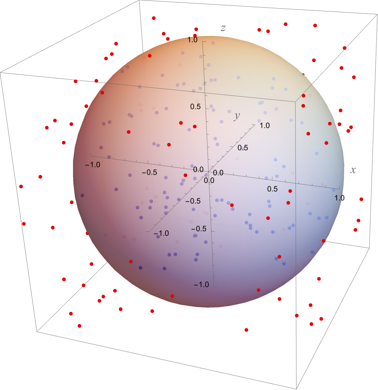
Figure 1: Illustration of the state space of a single qubit [$N=2$]. A random sample of 100 states that satsify the Bloch sphere inequality Eq. (113) is represented by the points in blue. Such points are necessarily located within the Bloch sphere. The red points correspond to a random sample of 100 states that satisfy Eq. (178), but do not satisfy the Bloch sphere inequality Eq. (113). Such points lie outside of the Bloch sphere, but within the classical state space defined by Eq. (178), which is bounded by the cube and includes the Bloch sphere as a subset.

where we use the bar to distinguish the classical probabilities $\bar{p}_{a}(s,t)$ from their quantum counterparts $p_{a}(s,t)$, and

$$p_{\mathrm{cl}}(\sigma_{x},\sigma_{y},\sigma_{z},t)=\int_{-\infty}^{\infty}\int_{-\infty}^{\infty}\int_{-\infty}^{\infty}\Theta(\sigma_{x}S_{x})\Theta(\sigma_{y}S_{y})\Theta(\sigma_{z}S_{z})\rho(S_{x},S_{y},S_{z},t)dS_{x}dS_{y}dS_{z}.$$ (177)

By definition, each component $\bar{p}_{a}(s,t)$ remains nonnegative at any arbitrary time $t$. Note that the classical state space defined by the set of points $\{\langle\sigma_{x}\rangle_{\mathrm{cl}},\langle\sigma_{y}\rangle_{\mathrm{cl}},\langle\sigma_{z}\rangle_{\mathrm{cl}}\}$, where

$$\langle\sigma_{a}\rangle_{\mathrm{cl}}\mathrel{\hbox to0.0pt{\raisebox{1.29167pt}{$\cdot$}\hss}\raisebox{-1.29167pt}{$\cdot$}}=(+1)\bar{p}_{a}(+1,t)+(-1)\bar{p}_{a}(-1,t),$$ (178)

is a cube with a side length of $2$, centered at the origin, with each side parallel to the $x$, $y$, and $z$ axis. Embedded within this cube is the Bloch sphere with a radius of $1$, making contact with the cube at its extremities, as illustrated in Fig. 1. Any point that is located inside of the cube, yet not within the Bloch sphere (such as those indicated in red in Fig. 1), corresponds to a probability distribution that does not align with our traditional understanding of quantum mechanics.

Returning to quantum dynamics as delineated by Eq. (25), the evolution of a single-qubit system is described by

$$\frac{d}{dt}\left[\begin{array}[c]{c}p_{x}(+1,t)\\ p_{x}(-1,t)\\ p_{y}(+1,t)\\ p_{y}(-1,t)\\ p_{z}(+1,t)\\ p_{z}(-1,t)\end{array}\right]=\left[\begin{array}[c]{cccccc}0&0&-B_{z}/2&B_{z}/2&B_{y}/2&-B_{y}/2\\ 0&0&B_{z}/2&-B_{z}/2&-B_{y}/2&B_{y}/2\\ B_{z}/2&-B_{z}/2&0&0&-B_{x}/2&B_{x}/2\\ -B_{z}/2&B_{z}/2&0&0&B_{x}/2&-B_{x}/2\\ -B_{y}/2&B_{y}/2&B_{x}/2&-B_{x}/2&0&0\\ B_{y}/2&-B_{y}/2&-B_{x}/2&B_{x}/2&0&0\end{array}\right]\left[\begin{array}[c]{c}p_{x}(+1,t)\\ p_{x}(-1,t)\\ p_{y}(+1,t)\\ p_{y}(-1,t)\\ p_{z}(+1,t)\\ p_{z}(-1,t)\end{array}\right].$$ (197)

In contrast to the probabilities $\bar{p}_{a}(s,t)$ in the case of classical dynamics described by Eq. (167), which are always nonnegative, $p_{a}(s,t)$ can take on negative values in the quantum dynamics described by Eq. (197), even when the same initial condition is chosen for both equations. The presence of negative probability components $p_{a}(s,t)$ constitutes a direct indication for the violation of NM in quantum dynamics for the initial state with $\vec{p}_{\mathrm{cl}}(0)$ in Eq. (176).

Next, let us reconsider the measure $\gamma_{n,k}$ introduced in Eq. (111) to quantify the violation of NM for a single qubit. Unlike the case of large $N$, we can easily determine its value for $N=2$. Let us assume that the initial state of the qubit is described by the probability vector $\vec{p}$ of Eq. (122). After performing a measurement of $\hat{\sigma}_{a}$ at $t=0$ and obtaining the result $s=\pm 1$, we define a pseudo-density matrix denoted by $\hat{\rho}_{a,s}^{\prime}$. As per Eq. (109), this matrix is described by the expression

$$\hat{\rho}^{\prime}_{a,s}=\frac{1}{2}\left(\hat{I}+s\hat{\sigma}_{a}+\sum_{a^{\prime}\neq a}\operatorname{Tr}\left[\hat{\sigma}_{a^{\prime}}\hat{\rho}(0)\right]\hat{\sigma}_{a^{\prime}}\right).$$ (198)

Expanding Eq. (198) with respect to the identity matrix and the Pauli matrices [cf. Eq. (112)] as

$$\hat{\rho}^{\prime}_{a,s}=\frac{1}{2}\left(\hat{I}+\left\langle\sigma_{x}\right\rangle^{\prime}_{a,s}\hat{\sigma}_{x}+\left\langle\sigma_{y}\right\rangle^{\prime}_{a,s}\hat{\sigma}_{y}+\left\langle\sigma_{z}\right\rangle^{\prime}_{a,s}\hat{\sigma}_{z}\right)$$ (199)

yields the following relations:

$$\left\langle\sigma_{a}\right\rangle^{\prime}_{a,s} =s,$$ (200)

$$\left\langle\sigma_{b\neq a}\right\rangle^{\prime}_{a,s} =\operatorname{Tr}\left[\hat{\sigma}_{b}\hat{\rho}(0)\right],$$ (201)

where $a,b\in\{x,y,z\}$ here and in what follows. Note that $\hat{\rho}_{a,s}^{\prime}$ can possess a negative eigenvalue. Indeed, the two eigenvalues of the $2\times 2$ matrix $\hat{\rho}^{\prime}_{a,s}(0)$ are given explicitly by

(202)

Consequently, the NM violation measure $\gamma_{a,s}$ of Eq. (111) with $s=\pm 1$ is evaluated as

The value of $\gamma_{a,s}$ quantifies the extent to which the NM post-measurement state differs from physical post-measurement states. Since some of the NM post-measurement states are not realized in the experiment, $\gamma_{a,s}$ itself does not qualify as a physical quantity. However, it is closely related to a physical quantity $\Delta$ which can be determined in experiments, as elucidated below.

It follows from Eqs. (200) and (201) that the squared expectation values of the Pauli matrices fulfill the following relation:

$$\begin{aligned} &\left(\left\langle\sigma_{x}\right\rangle^{\prime}_{a,s}\right)^{2}+\left(\left\langle\sigma_{y}\right\rangle^{\prime}_{a,s}\right)^{2}+\left(\left\langle\sigma_{z}\right\rangle^{\prime}_{a,s}\right)^{2}\\ &\hskip 28.45274pt=1+\sum\limits_{b\neq a}\Big{(}\!\operatorname{Tr}\left[\hat{\sigma}_{b}\hat{\rho}(0)\right]\!\Big{)}^{2}.\end{aligned}$$ (204)

Note that, since $\big{(}\!\left\langle\sigma_{x}\right\rangle^{\prime}_{a,s}\!\big{)}^{2}+\big{(}\!\left\langle\sigma_{y}\right\rangle^{\prime}_{a,s}\!\big{)}^{2}+\big{(}\!\left\langle\sigma_{z}\right\rangle^{\prime}_{a,s}\!\big{)}^{2}>1$, the vector $\big{[}\!\left\langle\sigma_{x}\right\rangle^{\prime}_{a,s},\left\langle\sigma_{y}\right\rangle^{\prime}_{a,s},\left\langle\sigma_{z}\right\rangle^{\prime}_{a,s}\!\big{]}$ lies outside of the Bloch sphere. From Eqs. (203) and (204), $\gamma_{a,-s}$ is found to be equivalent to $\gamma_{a,s}$. In what follows, we therefore let $\gamma_{a}$ represent $\gamma_{a,s}$ given by

$$\gamma_{a}\equiv\gamma_{a,s}\mathrel{\hbox to0.0pt{\raisebox{1.29167pt}{$\cdot$}\hss}\raisebox{-1.29167pt}{$\cdot$}}=\frac{1}{2}\left(\sqrt{1+\sum_{b\neq a}\big{(}\!\operatorname{Tr}\left[\hat{\sigma}_{b}\hat{\rho}(0)\right]\!\big{)}^{2}}-1\right).$$ (205)

The expectation values prior to the measurement are denoted by $\left\langle\sigma_{b}(0)\right\rangle=\operatorname{Tr}\left[\hat{\sigma}_{b}\hat{\rho}(0)\right]$. Upon solving Eq. (205), the following set of three equations is obtained:

$$\left\langle\sigma_{x}(0)\right\rangle^{2}+\left\langle\sigma_{y}(0)\right\rangle^{2} =4\gamma_{z}(1+\gamma_{z}),$$ (206)

$$\left\langle\sigma_{y}(0)\right\rangle^{2}+\left\langle\sigma_{z}(0)\right\rangle^{2} =4\gamma_{x}(1+\gamma_{x}),$$ (207)

$$\left\langle\sigma_{z}(0)\right\rangle^{2}+\left\langle\sigma_{x}(0)\right\rangle^{2} =4\gamma_{y}(1+\gamma_{y}).$$ (208)

The summation of Eqs. (206)–(208) yields

$$\left\langle\sigma_{x}(0)\right\rangle^{2}+\left\langle\sigma_{y}(0)\right\rangle^{2}+\left\langle\sigma_{z}(0)\right\rangle^{2}=2\sum_{a}\gamma_{a}(1+\gamma_{a}).$$ (209)

In conjunction with the Bloch sphere condition Eq. (113) for the initial state $\hat{\rho}(0)$ [i.e. the left-hand side of Eq. (209)], this relation establishes the following upper bound for the violation of NM:

$$\sum_{a}\gamma_{a}(1+\gamma_{a})\leqslant\frac{1}{2}.$$ (210)

Based on Eq. (209), it is possible to derive an analogous inequality for the measured observables. Upon observing $\hat{\sigma}_{a}$, the averaged post-measurement state is given by

$$\hat{\rho}_{a}=\sum_{s=\pm 1}\hat{P}_{a,s}\hat{\rho}(t=0)\hat{P}_{a,s},$$ (211)

where $\hat{P}_{a,s}=|s\rangle_{a}\langle s|_{a}$ are the projection matrices of $\hat{\sigma}_{a}$ associated with the eigenvalues $s=\pm 1$. The deviation of the expectation value of $\hat{\sigma}_{b}$ quantifies the backreaction of the measurement and is given by

$$\delta\sigma_{b}(a)=\left\langle\sigma_{b}\right\rangle^{\prime}_{a}-\left\langle\sigma_{b}(0)\right\rangle=\operatorname{Tr}\left[\hat{\sigma}_{b}\hat{\rho}_{a}\right]-\operatorname{Tr}\left[\hat{\sigma}_{b}\hat{\rho}(0)\right].$$ (212)

Based on this expression, we can introduce the measure $\Delta$ as follows:

$$\begin{aligned} \Delta&\mathrel{\hbox to0.0pt{\raisebox{1.29167pt}{$\cdot$}\hss}\raisebox{-1.29167pt}{$\cdot$}}=\frac{1}{3}\sum_{a}\sum_{b}\big{(}\delta\sigma_{b}(a)\big{)}^{2}\\ &=\frac{1}{3}\sum_{a}\sum_{b}\big{(}\!\left\langle\sigma_{b}\right\rangle^{\prime}_{a}-\left\langle\sigma_{b}(0)\right\rangle\!\big{)}^{2}.\end{aligned}$$ (213)

As alluded to previously, this quantity can be determined by experiments. Using Eq. (211) and the cyclic property of the matrix trace, we obtain

$$\delta\sigma_{b}(a)=\operatorname{Tr}\left[\left(\sum_{s=\pm 1}\hat{P}_{a,s}\hat{\sigma}_{b}\hat{P}_{a,s}-\hat{\sigma}_{b}\right)\hat{\rho}(0)\right].$$ (214)

It turns out that

$$\sum_{s=\pm 1}\hat{P}_{a,s}\hat{\sigma}_{b\neq a}\hat{P}_{a,s}=0$$ (215)

is satisfied for the Pauli matrices. From Eqs. (214)–(215), it follows that

$$\delta\sigma_{b}(a)=\left(\delta_{ab}-1\right)\left\langle\sigma_{b}(0)\right\rangle.$$ (216)

This yields

$$\sum_{a}\sum_{b}\big{(}\delta\sigma_{b}(a)\big{)}^{2}=2\left(\left\langle\sigma_{x}(0)\right\rangle^{2}+\left\langle\sigma_{y}(0)\right\rangle^{2}+\left\langle\sigma_{z}(0)\right\rangle^{2}\right).$$ (217)

From Eqs. (209), (213), and (217), we obtain a useful formula relating the abstract quantity $\gamma_{a}$ to the experimentally accessible $\Delta$ given by

$$\Delta=\frac{4}{3}\sum_{a}\gamma_{a}\left(1+\gamma_{a}\right).$$ (218)

If $\Delta>0$, the single qubit in the initial state $\hat{\rho}(0)$ does not conform to NM. Put simply, the relation in Eq. (218) quantifies the extent to which the quantum world differs from a world with $\gamma_{a}=0$ where NM holds.

Next, we present examples of qubit quantum states to check the breakdown of NM. First, consider the maximally mixed state described by $\hat{\rho}(0)=\hat{I}/2$. The corresponding probability vector is given by

$$\vec{p}=\left[\begin{array}[c]{c}p_{x}(+1,0)\\ p_{x}(-1,0)\\ p_{y}(+1,0)\\ p_{y}(-1,0)\\ p_{z}(+1,0)\\ p_{z}(-1,0)\end{array}\right]=\left[\begin{array}[c]{c}\text{\textonehalf}\\ \text{\textonehalf}\\ \text{\textonehalf}\\ \text{\textonehalf}\\ \text{\textonehalf}\\ \text{\textonehalf}\end{array}\right].$$ (231)

Prior to the measurement of $\hat{\sigma}_{a}$, all expectation values are null, i.e. $\left\langle\sigma_{a}(0)\right\rangle=p_{a}(+1,0)-p_{a}(-1,0)=\text{\textonehalf}-\text{\textonehalf}=0\;\forall a$. If the result $\sigma_{x}=+1$ is observed after an NM measurement of $\hat{\sigma}_{x}$ is performed, the probability vector becomes

$$\vec{p}\mkern 2.0mu\vphantom{p}^{\prime}_{x,+1}=\left[\begin{array}[c]{c}p_{x}^{\prime}(+1)_{x,+1}\\ p_{x}^{\prime}(-1)_{x,+1}\\ p_{y}^{\prime}(+1)_{x,+1}\\ p_{y}^{\prime}(-1)_{x,+1}\\ p_{z}^{\prime}(+1)_{x,+1}\\ p_{z}^{\prime}(-1)_{x,+1}\end{array}\right]=\left[\begin{array}[c]{c}1\\ 0\\ \text{\textonehalf}\\ \text{\textonehalf}\\ \text{\textonehalf}\\ \text{\textonehalf}\end{array}\right].$$ (244)

The associated state $\hat{\rho}_{x,+1}^{\prime}$ is an eigenstate given by $|+_{x}\rangle\langle+_{x}|$ of $\hat{\sigma}_{x}$, thus establishing it as a quantum state that is compatible with the NM postulate. Hence, the NM violation measure for this particular state vanishes, i.e. $\gamma_{x,+1}=0$, and thus also $\Delta_{x,+1}=0$ by virtue of Eq. (218). Similarly, measurements of other components $\hat{\sigma}_{a}$ yield analogous quantum states. A single-qubit system whose initial state is described by $\hat{\rho}(0)=\hat{I}/2$ is therefore compatible with NM.

On the other hand, if an NM measurement of $\hat{\sigma}_{y}$ is performed on the initial state $\hat{\rho}(0)=|+_{x}\rangle\langle+_{x}|$ and the result $\sigma_{y}=+1$ is observed, the probability vector becomes

$$\vec{p}\mkern 2.0mu\vphantom{p}^{\prime}_{y,+1}=\left[\begin{array}[c]{c}p_{x}^{\prime}(+1)_{y,+1}\\ p_{x}^{\prime}(-1)_{y,+1}\\ p_{y}^{\prime}(+1)_{y,+1}\\ p_{y}^{\prime}(-1)_{y,+1}\\ p_{z}^{\prime}(+1)_{y,+1}\\ p_{z}^{\prime}(-1)_{y,+1}\end{array}\right]=\left[\begin{array}[c]{c}1\\ 0\\ 1\\ 0\\ \text{\textonehalf}\\ \text{\textonehalf}\end{array}\right].$$ (257)

Similarly, if the result $\sigma_{y}=-1$ is observed instead of $\sigma_{y}=+1$, the probability vector becomes

$$\vec{p}\mkern 2.0mu\vphantom{p}^{\prime}_{y,-1}=\left[\begin{array}[c]{c}p_{x}^{\prime}(+1)_{y,-1}\\ p_{x}^{\prime}(-1)_{y,-1}\\ p_{y}^{\prime}(+1)_{y,-1}\\ p_{y}^{\prime}(-1)_{y,-1}\\ p_{z}^{\prime}(+1)_{y,-1}\\ p_{z}^{\prime}(-1)_{y,-1}\end{array}\right]=\left[\begin{array}[c]{c}1\\ 0\\ 0\\ 1\\ \text{\textonehalf}\\ \text{\textonehalf}\end{array}\right].$$ (270)

Since $\vec{p}\mkern 2.0mu\vphantom{p}^{\prime}_{y,\pm 1}$ does not adhere to the Bloch sphere condition prescribed by Eq. (115), the associated states $\hat{\rho}^{\prime}_{y,\pm 1}$ inevitably violate the NM postulate. Indeed, the corresponding NM violation measure $\gamma_{y,\pm 1}$ takes on positive values, namely

$$\gamma_{y,\pm 1}=\frac{\sqrt{2}-1}{2}.$$ (271)

In this case, under appropriate selection of $B_{a}$ in Eq. (123), solving Eq. (197) reveals that some negative probability components $p_{a}(s,t)$ appear at a future time $t$. The negativity of the probability components $p_{a}(s,t)$ therefore serves as evidence illustrating the violation of NM, and thus ultimately LGIs.

IV N-Level Systems

In a single-qubit system, every point contained within the Bloch sphere corresponds to a quantum state that can be realized in experiments. Analogous to the Pauli operators $\hat{\sigma}_{a}$ for $N=2$, one can introduce $N^{2}-1$ observables $\hat{\lambda}_{n}$ to describe the dynamics of generic $N$-level quantum systems, cf. Eqs. (7)–(11). The $N$-level generalization of the Bloch sphere defining inequality Eq. (113) is

$$\sum_{n=1}^{N^{2}-1}\left\langle\lambda_{n}\right\rangle^{2}\leqslant N-1.$$ (272)

Analogous to the single-qubit case with $N=2$, a saturation of this inequality corresponds to a pure quantum state. However, in contrast to the single-qubit case, a subset of the set of points $\{\left\langle\lambda_{1}\right\rangle,\ldots,\left\langle\lambda_{N^{2}-1}\right\rangle\}$ that satisfy the relation prescribed by Eq. (272) does not describe valid quantum states [19]. Consider, for instance, the quantum state described by $\hat{\rho}_{1}=\sum_{k}p_{k}|k\rangle\langle k|\geqslant 0$. Then, the vector $\vec{\lambda}_{1}=\left[\left\langle\lambda_{1}\right\rangle_{1},\ldots,\left\langle\lambda_{N^{2}-1}\right\rangle_{1}\right]$ defined by $\left\langle\lambda_{n}\right\rangle_{1}=\operatorname{Tr}\big{[}\hat{\lambda}_{n}\hat{\rho}_{1}\big{]}$ provides the Bloch representation of $\hat{\rho}_{1}$, i.e.

$$\hat{\rho}_{1}=\frac{1}{N}\hskip 1.42262pt\Bigg{(}\hat{I}+\sum_{n=1}^{N^{2}-1}\left\langle\lambda_{n}\right\rangle_{1}\hat{\lambda}_{n}\Bigg{)}.$$ (273)

Another quantum state $\hat{\rho}_{2}$ given by

$$\hat{\rho}_{2}=\frac{1}{N}\hskip 1.42262pt\Bigg{(}\hat{I}+\sum_{n=1}^{N^{2}-1}\left\langle\lambda_{n}\right\rangle_{2}\hat{\lambda}_{n}\Bigg{)}$$ (274)

should satisfy

$$\begin{aligned} \operatorname{Tr}\left[\hat{\rho}_{1}\hat{\rho}_{2}\right]&=\sum_{k}p_{k}\langle k|\hat{\rho}_{2}|k\rangle\\ &=\frac{1}{N}\hskip 1.42262pt\Bigg{(}1+\sum_{n=1}^{N^{2}-1}\left\langle\lambda_{n}\right\rangle_{1}\left\langle\lambda_{n}\right\rangle_{2}\Bigg{)}\geqslant 0.\end{aligned}$$ (275)

Hence $\vec{\lambda}_{2}=\left[\left\langle\lambda_{1}\right\rangle_{2},\ldots,\left\langle\lambda_{N^{2}-1}\right\rangle_{2}\right]$ obeys the following necessary condition:

$$\vec{\lambda}_{1}\cdot\vec{\lambda}_{2}=\sum_{n=1}^{N^{2}-1}\left\langle\lambda_{n}\right\rangle_{1}\left\langle\lambda_{n}\right\rangle_{2}\geqslant-1.$$ (276)

It follows from Eq. (276) that, when $\hat{\rho}_{1}$ is a pure state satisfying $\sum_{n=1}^{N^{2}-1}\left\langle\lambda_{n}\right\rangle^{2}_{1}=N-1$, a pure quantum state $\hat{\rho}_{2}$ which meets the condition $\left\langle\lambda_{n}\right\rangle_{2}=-\left\langle\lambda_{n}\right\rangle_{1}$ does not exist for $N\geqslant 3$. Consequently, the higher-dimensional generalization of the Bloch sphere inequality given in Eq. (272) does not suffice to guarantee physically viable quantum states described by a positive semidefinite operator $\hat{\rho}\geqslant 0$. The implication here is that the state space characterized by $\left[\left\langle\lambda_{1}\right\rangle,\ldots,\left\langle\lambda_{N^{2}-1}\right\rangle\right]$ is a rather intricate manifold. Therefore, for large values of $N$ it is in general quite difficult to determine whether a given vector $\left[\left\langle\lambda_{1}\right\rangle,\ldots,\left\langle\lambda_{N^{2}-1}\right\rangle\right]$ corresponds to a valid quantum state or not since this requires the numerical diagonalization of $\hat{\rho}^{\prime}(0)$. Similarly, for large $N$ it is a numerically difficult task to check if a given probability vector of the form of Eq. (35) describes a valid quantum state or not (recall that such a vector comprises $N(N^{2}-1)$ components). In order to alleviate this difficulty, we propose to adopt a machine learning method.

V State Classification
      with Machine Learning

The aim of our proposed machine learning method is to train an algorithm in the classification of quantum states as either NM-conforming or NM-violating based on their associated probability vectors of the form given by Eq. (35). Such vectors consist of $(N^{2}-1)$ probability tuples $[P_{1},\ldots,P_{N^{2}-1}]$, each containing $N$ entries $[p_{n}(1,t),\ldots,p_{n}(N,t)]$ satisfying [cf. Eqs. (16) and (17)]

$$\sum\limits_{k}^{N}p_{n}(k,t)=1,\quad p_{n}(k,t)>0\qquad\forall\;n,k$$ (277)

with $n\in\{1,\ldots,N^{2}-1\}$ and $k\in\{1,\ldots,N\}$. The first step in our approach is the generation of training data that can be used for supervised learning. Since our goal is to distinguish quantum states that conform to NM from those that violate NM, we generate two distinct probability vector training data sets; the first containing exclusively vectors associated with NM-conforming states, and the second containing exclusively vectors associated with NM-violating states.

V.A Training Data Generation

For any arbitrary $N\geqslant 2$, we work with the generalized Gell-Mann matrix basis (GGMMB) [20] and generate pseudo-density states according to the spectral decomposition of Eq. (110), where the projectors $\hat{P}^{\prime}_{m}(n,k)$ are constructed from pseudo-randomly generated $N$-dimensional vectors that are orthonormalized via the Gram-Schmidt process. The individual components of the probability vectors are then generated via Eq. (16), where this time the projectors $\hat{P}_{n}(k)$ are those associated with the elements of the GGMMB. The difference in the generation of probability vectors for the NM-conforming vs. the NM-violating data set lies in the pseudo-random generation of the coefficients $p^{\prime}_{m}(n,k)$ of Eq. (110): while the normalization condition Eq. (17) is always satisfied for each of the $N$ probability tuples in both data sets, negative values $p^{\prime}_{m}(n,k)<0$ are permitted in the generation of probability vectors associated with quantum states that violate the NM postulate to reflect the fact that the spectrum of the post-measurement density matrix [cf. Eq. (103)] may contain negative eigenvalues (and thus cannot describe a physically valid quantum state if NM is assumed to hold). This may ultimately result in probability vectors with negative components $p_{n}(k,t)<0$. However, since this contradicts the second requirement stipulated by Eq. (277), such vectors are then discarded, and only those satisfying both conditions are passed onto the NM-violating training data set. Fig. 2 illustrates the distribution of the NM violation measure $\gamma_{n,k}$ [Eq. (111)] for 1,000 pseudo-randomly generated probability vectors in the NM-violating data sets of $N\in\{2,3,4,5\}$.

V.B Supervised Learning and
        Probability Vector Classification

Supervised learning is a type of machine learning algorithm that infers a function from labeled training data. Training data sets are typically composed of pairs in which an input object is assigned a desired output value. For our purposes, the supervised learning task corresponds to a classification task, and the inferred function is a classifier function $\mathcal{C}$, i.e. a map $\mathrm{out}=\mathcal{C}(\mathrm{in})$ between input objects (i.e. probability vectors) and output values (i.e. the state classification).

An example implementation of our proposed machine learning methodology is openly available in the Github repository listed as Ref. [22], including a separate file documenting the statistical distributions underlying the pseudo-random generation of the coefficients $p^{\prime}_{m}(n,k)$ for both training data sets. The code provided in this repository is written in Mathematica 13 [23], and the supervised learning task is performed by Mathematica’s built-in “Classify[]” function. In our example implementation, the training data set is generated such that all probability vectors from the NM-conforming [NM-violating] data set are assigned the desired output value 0 [1]. The resulting classifier function takes then an $N(N^{2}-1)$-dimensional probability vector as input and returns either 0 or 1 based on whether it has determined the state associated with the input vector to be of the NM-conforming or the NM-violating type. As a sanity check and to test the robustness of the classifier, we can feed the classifier function probability vectors for which the classification is known a priori (e.g. through independent manual determination of NM conformity) and evaluate its performance based on the accuracy of its ouput classifications.

We stress that the sole intention of the provided code is to serve as a proof-of-principle implementation for our proposed machine learning methodology. As such, several refinements and extensions will be required in order to model real experimental applications and/or realistic large-$N$ systems.

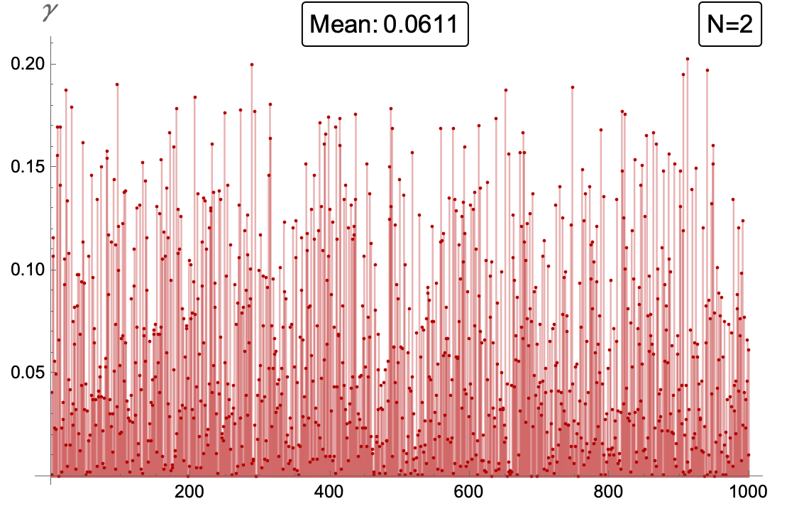
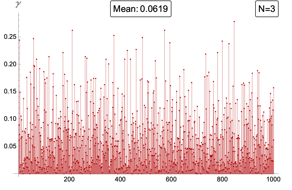
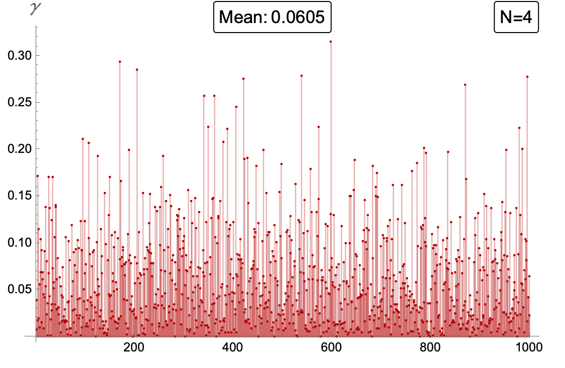
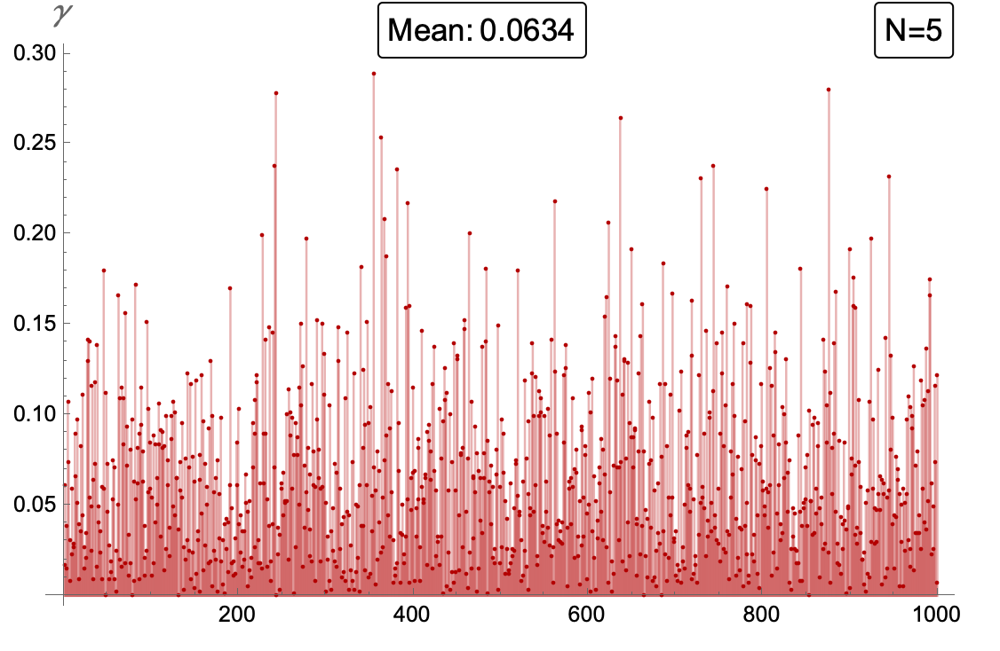
Figure 2: Distribution of the NM violation measure $\gamma_{n,k}$ [Eq. (111)] computed for 1,000 pseudo-randomly generated non-classical (i.e. NM-violating) states for $N\in\{2,3,4,5\}$ and their respective mean values $\bar{\gamma}=\frac{1}{1000}\sum_{i}^{1000}\gamma_{i}$.

VI Conclusions

Starting from the density operator form of the Schrödinger equation [Eq. (6)], we derive a formally equivalent probability vector representation [Eq. (25)] which describes the quantum dynamics of a system in terms of the probabilities associated with its observables. Our analysis demonstrates that the probability vector representation is uniquely suited to study features in the evolution of non-classical systems that are relevant with respect to the NM postulate and its possible violation. Due to the specific form of Eq. (65), an exact diagonalization of the Hamiltonian is not required in this formalism, which has many advantages when $N$ is large.

After an NM measurement is performed, the post-measurement density operator may no longer be positive semidefinite (as evidenced by the fact that its spectrum may contain negative eigenvalues), which is indicative of NM violations and a dynamical evolution that cannot be understood classically (in the sense of being compatible with both MR and NM). While the negativity of quasiprobabilities has previously been considered as an indicator of quantumness in the Wigner–Weyl representation [9], the difference in our approach is that all initial probabilities are always nonnegative for both classical and quantum dynamics. This allows us to pinpoint what physical consequences the requirement of no backreaction that is encoded in the NM postulate entails.

The extent to which NM is violated by quantum dynamics is ultimately determined by the evolution of probability distributions associated with the observables of the system under consideration and can be quantified using the measure defined in Eq. (111). For single-qubit systems, we derive its explicit relationship to the backreaction of a measurement (i.e. the deviation from the NM postulate) [Eqs. (205), (213), and (218)].

As motivated by our argumentation in Sec. II, we expect our scheme to be more efficient computationally compared to conventional equation-solving approaches, particularly for the dynamics of large-$N$ systems. In this regime, the exploration of machine learning techniques (especially big data methods) appears to hold a lot of promise. The explicit treatment of large-$N$ systems (e.g. $N\simeq 2^{10^{3}}\!\mathrm{-}2^{10^{4}}$ in condensed matter systems) including their possible experimental realization(s) will be considered in future works.