Unveiling diverse nature of core collapse supernovae

THESIS
Submitted For the Degree of
DOCTOR OF PHILOSOPHY
IN
PHYSICS
by
Amar Aryan
DEPARTMENT OF PHYSICS
DEEN DAYAL UPADHYAYA GORAKHPUR UNIVERSITY
GORAKHPUR-273009 (U.P.) INDIA

Research Centre
ARYABHATTA RESEARCH INSTITUTE OF OBSERVATIONAL SCIENCES (ARIES)
MANORA PEAK, NAINITAL-263001, INDIA

SEPTEMBER 2023

Dedicated to,

My Dada ji …

Acknowledgements

The Journey of my academic life commenced many years ago at “Middle School Kubri”, a government school in our village named “Kubri”. I vividly recall the unwavering encouragement and motivation I received from my teachers (among others) Sita Ram sir, Devnandan sir, and Sadhu sir. Subsequently, for my secondary education (10th), I got admission to “Gurukul Shikshalay”, a school near our village. I consider myself fortunate to have had the opportunity to learn from exceptional teachers, including Manoj sir, Deglal sir, Chandrika sir, Ravi sir, Akhilesh sir, Parvej sir, Pawan sir and others. They instilled a strong moral compass and laid the foundation within me for my academic success ahead.

In the pursuit of higher education, I came to Delhi in 2009. From my senior secondary (12th) school days through my bachelor’s and master’s degrees, I met numerous teachers and professors who provided unwavering support and motivation. I express my heartfelt gratitude to each one of them. I thank Meena sir from my senior secondary school for his support, motivation, and guidance. I am also grateful to Mukharjee sir for his assistance during my B.Sc college years. Moreover, I consider myself extremely fortunate to have attended lectures delivered by esteemed individuals such as Prof. Daya Shankar Kulshreshtha, Prof. Patrick Das Gupta, Prof. Shobhit Mahajan, Prof. H. P. Singh, Prof. T. R. Seshadri, Prof. Supriya Kar, Dr. Ashutosh Bhardwaj, Dr. Saurabh Sur, and others during my M.Sc program. I extend my heartfelt thanks to all the professors and lecturers who enriched my educational Journey during my M.Sc days.

Upon finishing my M.Sc., I commenced my Journey at Aryabhatta Research Institute of Observational Sciences (ARIES) on July 13th, 2018. I embarked as a Junior Research Fellow to pursue PhD, under the esteemed guidance of Dr. Shashi Bhushan Pandey. I extend my heartfelt gratitude to my PhD supervisor, Dr. Shashi Bhushan Pandey, as well as my co-supervisor, Prof. Sugriva Nath Tiwari, for their unwavering support, motivation, and guidance throughout this remarkable Journey. Their invaluable suggestions and directions were pivotal in completing this thesis. I am profoundly thankful to them for allowing me to explore the intellectual curiosity within my research and establish a solid foundation. I will forever appreciate the encouragement and excellent opportunities provided by my supervisor, Dr. S. B. Pandey, which allowed me to collaborate with eminent experts in the field of supernova research. I am grateful to Prof. Alexei V. Filippenko, Dr. Weikang Zheng, Prof. Keiichi Maeda, Prof. Jozsef Vinko, Prof. Dipankar Bhattacharya, and Prof. David A. H. Buckley for their constant support, suggestions and guidance throughout this beautiful Journey. I also acknowledge Prof. Craig Wheeler and Prof. Van Dyk Schuyler for valuable discussions regarding supernova observations and science. It was really a great experience for me to work in active collaboration with these eminent researchers.

I am very thankful to Ryoma Ouchi, Isaac Shivvers, Heechan Yuk, Sahana Kumar, Samantha Stegman, Goni Halevi, Timothy W. Ross, Carolina Gould, Sameen Yunus, Raphael Baer-Way, Asia deGraw, Dr. Abhay Pratap Yadav, Dr. Brajesh Kumar, Thomas G. Brink, Andrew Halle, Jeffrey Molloy, Charles D. Kilpatrick, Sanyum Channa, Maxime de Kouchkovsky, Michael Hyland, Minkyu Kim, Kevin Hayakawa, Kyle McAllister, Andrew Rikhter, Benjamin Stahl, and Yinan Zhu for their kind support and help at various stages during my PhD. I immensely thank Ryoma Ouchi for his support in several projects. I am also very thankful to Dr. Abhay Pratap Yadav for his motivation and support.

I thank all the faculty members (Prof. Dipankar Banerjee, Dr. Brijesh Kumar, Dr. Alok Chandra Gupta, Dr. Jeewan C. Pandey, Dr. Ramakant S. Yadav, Dr. Saurabh, Dr. Kuntal Misra, Dr. Neelam Panwar, Dr. Indranil Chattopadhyay, Dr. Snehlata, Dr. Santosh Joshi, Dr. Yogesh Chandra Joshi, Dr. Manish K. Naja, Dr. Narendra Singh, Prof. Shantanu Rastogi, Prof. Ravi Shankar Singh, and others), engineers (Mohit Joshi, Ashish Kumar, Krishna Reddy B., Sanjit Sahu and others), post-doctoral fellows, research scholars (Prayag Bhaiya, Rahul Bhaiya, Teekendra, Atul, Vishnu, Vaibhav, Bakhtawar, Sumit and others), and staff members (Abhishek Sharma, Himanshu Vidyarthi, Ram Dayal Bhatt, Amar Singh Meena, Hemant Kumar, and others) of ARIES Nainital and the Department of Physics of DDU Gorakhpur University Gorakhpur profusely for their kind support throughout my study. In addition, I acknowledge the financial support of the BRICS grant DST/IMRCD/BRICS/Pilotcall/ProFCheap/2017(G). I also acknowledge the financial support from the Council of Scientific & Industrial Research (CSIR), India, under file no. 09/948(0003)/2020-EMR-I.

I thank my group members (Rahul Gupta, Amit Kumar, and Amit Kumar Ror). I also thank my other batch-mates (Raj, Mahendar, Nikita, and Akanksha), seniors (Mukesh bhaiya, Mridweeka di, Anjasha di, Ashwani bhaiya, Vineet bhaiya, Pankaj bhaiya, Amit, Ankur, Arpan, Krishan, Prajjwal, Aditya, Vinit, Jaydeep, and others), Juniors (Devanand, Mrinmoy, Bhavya, Kiran, Rahul, Shubham, Tushar, Nitin, Gurpreet, Naveen, Aayushi, Upasna, Shivangi, Dibya, Karan, Tarak, Srinivas, Vikrant, Monalisa, and others) and canteen members (specially, Darshan, Jagdish dajyu, and Ravi dajyu) at ARIES and Devasthal campus, who have made this Journey even more memorable.

My family is my most valuable asset. Without their unwavering support, I can hardly imagine my fate. The words of wisdom by my Dadaji, Late Jagdish Ram, always consistently steered me on the path of life. A promise made by me to my Papa, Late Birendra Kumar Kashyap, encouraged me to achieve several milestones, with many more yet to come. The unwavering support, motivation, and encouragement from my mummy, Smt. Yashoda Devi, have been a constant presence in my life. The support from my bhaiya, Shri Hira Lal and bhabhi, Smt. Soni Kashyap can not be expressed in mere words. My brother went above and beyond, doing nothing less than a father would do for his son. My two nephews Astitva and Manas kept me happy and entertained all the time. I also thank my two elder sisters, Paro di and Kanchan di, for their unwavering support and unconditional care, treating me as if I were their own child. I am thankful to Deepak Jija Ji and Anil Jija Ji for all their love and support. Their kids Aditya, Krishna, Saurya Sankar, and Alok Ranjan have also been my constant entertainment source. Their presence filled my life with joy. In 2014, I felt blessed when I met my love Urvashi Rathore. She is an inexhaustible source of motivation and has continuously provided me with selfless support in every situation. Her presence in my life has been a source of great comfort and strength.

I can never forget the support of my dear uncles, Late Chander dev Kashayp, Shri Surendra Kashyap, Shri Rohit Kashyap, and Shri Bhuneshwar Kashyap. I am really in debt to their love and affection, especially Sanhjhle Papa (Shri Surendra Kashyap). I extend a special thank you to Chhote chacha, Shri Bhuneshwar Kashyap for standing on my side on many difficult occasions. I am also thankful to my dadi ji, Smt. Koyali Devi and aunties, Kanta Devi, Geeta Devi, Kiran Devi and Sarita Devi for all their love and blessings. I am glad to mention the names of my cousins, Bablu bhaiya, Baby di, Chhoti bhaiya, Moti bhaiya, Pankaj bhaiya, Priya di, Kajri di, Akash, Asha, Prabha, Paras, Puja, Guddu, Mansi and Golu for their everlasting love and support. I extend a special thank you to Moti bhaiya for standing by my side in hard times. I thank Pinky di for her support. She always inspired me to achieve my goals. Thanks to Rajesh, Phupha Ji and Phuwa Ji for their love. I am very thankful to my maternal uncles, Shri Vasudeo Pandit, Shri Mathura Pandit, and Shri Sita Ram Pandit. I am also very grateful to Badi Mami, Manjhli Mami, and Chhoti Mami for their unconditional love and affection. I am also overwhelmed to thank my cousins from the maternal side, Sunil bhaiya, Deepak bhaiya, Pankaj, Seemu, Dinesh, Jitu, and Nikhil, for their support. I am also very thankful to Dr. Shashi Bhushan Pandey’s wife (ma’am) and their children for giving me a family environment at ARIES and serving us tasty food on numerous occasions.

Friends play a significant role in our lives as they profoundly impact our emotional, social, and personal well-being. I thank my village friends, Rahul (Chacha), Vikram, Vijay, Rakesh Rana, Rahul Rana, Raja Rana, Dara, Panga, Ajit, Ayodhya, Brabha and others. They always cheered each of my movements ahead. I also thank my Delhi friends, especially Lokesh, for their support. I spent a lot of good times with my friends Nitesh, Ashish, and Mukesh during my M.Sc program. During my PhD journey, whenever I visited Delhi, I had a delightful time staying with Kapildev, Avnish, and Nitesh. Exploring Vijay Nagar with them added to the joy of my stay.

My research Journey has been an exhilarating adventure, marked by high phases and setbacks too. Maintaining my sanity throughout this entire endeavour proved to be a formidable task. However, I consistently relied on my abilities and confidently tackled each new challenge. I am immensely grateful to everyone who supported and assisted me along this Journey. This thesis is a result of blessings from several individuals. Last but not least, I thank the almighty God for everything. I look forward to reaching many more remarkable milestones in my life.

— Amar

PREFACE

Core-collapse supernovae (CCSNe) are catastrophic astrophysical phenomena that occur during the last evolutionary stages of massive stars having initial masses $\gtrsim$ 8 M_⊙. These catastrophic events play a pivotal role in enriching our Universe with heavy elements and are also responsible for the birth of Neutron stars and stellar mass Black holes. Knowledge of the possible progenitors of CCSNe is fundamental to understanding these transient events. Additionally, the underlying circumstellar environment around possible progenitors and the physical mechanism powering the light curves of these catastrophic CCSN events also require careful investigations to unveil their nature. Based on the spectroscopic observational features, the CCSNe are primarily divided into H-rich and H-deficient categories. The H-rich CCSNe display unambiguous H-features in their spectra, while H-deficient CCSNe don’t. Type Ib SNe are a subclass of H-deficient CCSNe that lack prominent H-features in their spectra but display distinct He-feature.

The research work within the context of the present thesis is an attempt to investigate the possible progenitors, ambient media around the progenitors, and powering mechanisms behind the light curve of CCSNe. Particularly, fractional contributions of different elements, including hydrogen, the key element discriminating Type Ib and Type IIb SNe, are studied in detail. We also employed several powering mechanisms to decipher underlying physical mechanisms behind Type Ib and Type IIb SNe. We have employed observational data from several telescopes, state-of-the-art simulation modules, and 1-dimensional hydrodynamic codes for such investigations.

In this thesis, we have investigated the photometric and spectroscopic properties of two Type Ib CCSNe, namely, SN 2015ap and SN 2016bau. We aim to gain insight into their possible progenitors, the circumstellar environment surrounding them, and the powering mechanism for their light curve. We have analysed the photometric characteristics of the CCSNe mentioned above, encompassing their colour evolution, bolometric luminosity, photospheric radius, temperature, and velocity evolution. By analysing their light curves, we have computed the ejecta mass, synthesised nickel mass, and ejecta kinetic energy. Thus, the time domain astronomy of CCSNe is crucial to get insight into their several physical properties. Furthermore, we have modelled the spectra of SN 2015ap and SN 2016bau at different stages of their development and also compared their spectra with several other similar SNe. The P Cygni profiles of different lines present in the spectra are utilised to understand the velocity evolution of several line-emitting regions. The 1-dimensional stellar modelling of the possible progenitors and the comparison of the results of synthetic hydrodynamic explosions with actual observations indicate a 12 M_⊙ progenitor exploding in a solar metallicity region as the potential progenitor for SN 2015ap. In contrast, a slightly less massive star exploding in a solar metallicity environment is the expected progenitor for SN 2016bau. At the pre-SN stage, the mass of the progenitor of SN 2016bau lies close to the boundary between the SN and a non-SN phase.

Type IIb SNe are another subclass of CCSNe and are thought to bridge the gap between H-rich and H-deficient CCSNe. At first, their spectra reveal noticeable H-features, but after a few weeks, the H-features diminish while prominent He-features begin to emerge. Type Ib/IIb CCSNe progenitors retain no to very small amounts of hydrogen during their explosions. However, the correct estimation of the amount of hydrogen retained before explosion by the underlying CCSN progenitor is subjected to contamination by the uncertainties associated with determining the extinction and distance of the CCSN. The photometric and spectroscopic investigations of Type IIb CCSNe are necessary to understand their progenitors, ambient medium, and powering mechanisms. Such analyses also decipher their link with the H-rich and H-deficient CCSNe.

In the present research work, we have performed the photometric and spectroscopic investigation of a Type IIb SN 2016iyc. Our findings indicate that SN 2016iyc lies towards the lower end of the distribution compared to similar CCSNe in terms of inherent brightness. The light curve analysis indicates that SN 2016iyc produces a relatively smaller amount of ejecta mass and suffers low nickel mass production. Based on the photometric and spectroscopic behaviour of SN 2016iyc, we performed the stellar evolution of models having initial zero-age main-sequence (ZAMS) masses in the range of 9–14 M_⊙. The synthetic explosions of ZAMS star models with mass in the range of 12–13 M_⊙ having the pre-SN radius, $R_{\mathrm{0}}$ within (240–300) R_⊙, produce bolometric luminosity light curves and photospheric velocities that match well with actual observations. Additionally, ejecta mass $M_{\rm ej}=$ (1.89–1.93) M_⊙, explosion energy $E_{\rm exp}=$ (0.28–0.35) $\times 10^{51}$ erg, and $M_{\rm Ni}<0.09$ M_⊙, are in good agreement with observed estimations; thus, SN 2016iyc probably exploded from a progenitor lying towards the lower mass limits for SNe IIb. Additional hydrodynamic simulations have also been conducted to investigate the explosions of SN 2016gkg and SN 2011fu, aiming to compare intermediate- and high-luminosity examples among the extensively studied SNe Type IIb. The results obtained from modelling the potential progenitors and simulating the explosions of SN 2016iyc, SN 2016gkg, and SN 2011fu reveal a range of progenitor masses for SNe IIb. The range of progenitor masses for Type IIb SNe identified under the present research work lies well within the established range of progenitor masses for CCSNe.

After discussing the properties of H-deficient SNe and the behaviour of a Type IIb SN retaining an intermediate amount of H-envelope, we provide interesting properties of H-rich and H-deficient SNe together that originate from progenitors, each having a mass of 25 M_⊙ at ZAMS and zero metallicity. CCSNe from massive Population III (Pop III) stars are thought to have had an enormous impact on the early Universe. The SNe from Pop III stars were responsible for the initial enrichment of the early Universe with heavy elements. Pop III stars played a key role in cosmic re-ionization. Thus, the investigations of the stellar evolution of Pop III stars and resulting SNe are essential. This thesis presents the results of 1-dimensional stellar evolution simulations of a rotating Pop III star having an initial mass of 25 M_⊙. Starting from ZAMS, the models are evolved until the onset of core collapse. The rapidly rotating models exhibit violent and intermittent mass loss episodes following the main sequence stage. Notably, the Pop III models exhibit smaller pre-SN radii compared to the model with solar metallicity. Further, with models at the stage of the onset of core collapse, we perform the hydrodynamic simulations of the resulting SNe. As a consequence of the mass losses due to corresponding rotations and stellar winds, the resulting SNe span a class from weak H-rich to H-deficient CCSNe. This analysis demonstrates the substantial influence of initial stellar rotation on the evolution of massive stars and their resulting transients. Additionally, we observe that the absolute magnitudes of CCSNe originating from Pop III stars are much fainter compared to the ones originating from the star with solar metallicity. Based on the outcomes of our simulations, we conclude that within the range of explosion energies and nickel masses considered, these transient events exhibit very low luminosities. Consequently, detecting them at high redshifts would be a significant challenge.

Beyond discussing the CCSNe resulting from progenitors having ZAMS masses of 25 M_⊙ or less, we have also studied the stellar evolution of a massive 100 M_⊙ ZAMS star up to the onset of core collapse. Based on initial mass, mass loss rate, rotation and metallicity, the resulting transient could fall into any category, PISN, PPISN, Type IIP-like SNe, and several H-rich/H-deficient SNe showing ejecta-CSM interaction signatures. However, in the presented thesis, we have investigated the consequences of a non-rotating 100 M_⊙ ZAMS progenitor exploding into Type IIP-like CCSNe. We also have explored the effect of the variation of explosion energy and nickel mass on the light curves of resulting CCSNe.

The research work presented here has paved the way for new avenues of exploration within astronomy and astrophysics. Ultimately, we summarise our significant findings and discuss the potential prospects. We attempt to highlight the role of observations and simulations in synergistic investigations of transients. The increasing number of progenitor detections in high-resolution pre-explosion images and further refinement of available state-of-the-art stellar evolution codes would certainly protrude the knowledge of CCSNe.

Abbreviations, Notations and symbols

$\alpha$	Right Ascension
Å	Angstrom
ARIES	Aryabhatta Research Institute of observational SciencES
Ca II	Singly ionized Calcium
CCD(s)	Charge Couple Device(s)
CCSN(e)	Core-Collapse SuperNova(e)
CSM	Circum Stellar Material
$\delta$	Declination
DAOPHOT	Dominion Astrophysical Observatory Photometry
DOT	Devasthal Optical Telescope
DFOT	Devasthal Fast Optical Telescope
Eq	Equation
$\epsilon_{nuc}$	Specific Luminosity due to nuclear reactions
Fe II	Singly ionized Iron
Fe-core	Iron-core
Fig	Figure
FITS	Flexible Image Transport System
FoV	Field of View
FWHM	Full Width at Half Maxima
GRBs	Gamma-Ray Bursts
HN(e)	HyperNova(e)
H I	Neutral Hydrogen
H-envelope	Hydrogen-envelope
H-rich	Hydrogen-rich
He I	Neutral Helium
He-core	He-core
He-envelope	Helium-envelope
He-rich	Helium-rich
HST	Hubble Space Telescope
IRAF	Image Reduction Analysis Facilities
K	Kelvin
KN(e)	KiloNova(e)
MESA	Modules for Experiments in Stellar Astrophysics
Mg II	Singly ionized Magnesium
MJD	Modified Julian Date
Mpc	Mega-parsec
Myr	Millionyear
M⊙	Solar Mass
Na I D	Neutral Sodium Doublet
NIR	Near-infrared
NS(s)	Neutron Star(s)
O I	Neutral Oxygen
PSF	Point Spread Function
PISN(e)	Pair-Instability SN(e)
PPISN(e)	Pulsational Pair-Instability SN(e)
R⊙	Solar Radius
S II	Singly ionized Sulpher
SED(s)	Spectral Energy Distribution(s)
Si II	Singly ionized Silicon
SN(e)	SuperNova(e)
SNEC	SuperNova Explosion Code
ST	Sampurnanand Telescope
UT	Universal Time
UV	Ultraviolet
WD(s)	White Dwarf(s)
ZAMS	Zero-Age Main-Sequence

“Life is like riding a bicycle. To keep your balance, you must keep moving.”

—– Albert Einstein

Chapter 1 Introduction

Supernovae (SNe) are extreme astrophysical transient events occurring either when a White Dwarf (WD) is triggered into a runaway thermonuclear burning (Colgate, 1971; Arnett, 1979; Khokhlov et al., 1997) or during the last evolutionary stages of massive stars (Wilson et al., 1986; Hashimoto et al., 1993; Thielemann et al., 1996; Matzner & McKee, 1999). These catastrophic explosions represent the dynamical disruption of an entire star (Wheeler, 2012). SNe are among the brightest astrophysical explosions; thus, they play a crucial role in determining cosmological distances and verifying cosmological models (Baklanov et al., 2013). An astrophysical explosion occurs when magnetic, gravitational, or thermonuclear energy is released on dynamical timescales. The dynamical timescale is typically the sound-crossing time for the underlying system (Wheeler, 2012). Besides SNe, numerous explosive phenomena are continuously occurring in the Universe, including solar and stellar flares, eruptive phenomena in accretion disks, thermonuclear combustion on the surfaces of WDs and neutron stars (NSs), violent magnetic reconnection in NSs, cosmic gamma-ray bursts (GRBs) and kilonovae (KNe). Each of these explosions represents a different type and a different amount of energy released.

Several transient events are associated with compact object binary systems involving NSs and/or Black holes (BHs). These transient events include X-ray novae (Chen et al., 1997), X-ray bursters (Lewin et al., 1993), and soft gamma-ray repeaters (Mereghetti, 2008). Short-GRBs originating from the merger of NS–NS or NS–BH are another example of transient events involving a binary system of NS or/and BH (Lee et al., 2005; Murguia-Berthier et al., 2017; Abbott et al., 2017a; Lipunov et al., 2017). Additionally, KNe are a class of transient events that are also associated with such binary merger events (Metzger, 2017, 2019).

In contrast to the compact object binary systems mentioned above, the binary systems composed of a WD orbiting a companion star form a class of variable objects known as cataclysmic variables (CVs). There are two mechanisms through which the outbursts of radiant energy in CVs occur. The mechanism involving an accretion disk results in a “dwarf nova” (Smak, 1971; Osaki, 1974) while the other mechanism involving thermonuclear burning on the surface of WD results in “classical novae and recurrent novae” (Starrfield et al., 1974; Schaefer, 2010; Kato & Hachisu, 2012). The outbursts in the accretion disk resulting in a “dwarf nova” is rather a dramatic event than an explosion as the energy released is not on a dynamic scale. SNe are much more powerful events than novae. A detailed review of SNe is presented in the next section.

1.1 Supernovae

SNe are extreme catastrophic stellar explosions whose effects pervade the whole of astronomy (Murdin & Murdin, 1985). SNe explosions are so bright that they can outshine their host galaxy. These cataclysmic transient events enrich the Universe by creating and spreading heavier chemical elements (Matteucci & Greggio, 1986; Kawata & Gibson, 2003; Greif et al., 2007), trigger the star formations (Herbst & Assousa, 1977, 1978; van Dyk, 1992; Chiaki et al., 2013), and are also responsible for the birth of several compact objects including, NSs and BHs (Schramm & Arnett, 1975; Baumgarte et al., 1995; Woosley & Timmes, 1996; Israelian et al., 1999; Beacom et al., 2001).

1.1.1 History of supernovae observations in ancient and modern astronomy

$\bullet$ Ancient SNe observations: According to Joglekar et al. (2011), the oldest possible supernova (SN) record dates back to around 4600 $\pm$ 2000 BC, observed by unknown Indian observers. The name of the possible recorded SN is “HB9” (Joglekar et al., 2011). Following Murdin & Murdin (1985), the SN in the year AD 185 occurred in the Centaurus constellation and is the oldest ever recorded SN by humankind. Evidence indicates that two Roman chronicles also reference the SN that the Chinese recorded in AD 185. Further, in the year AD 386, there are recorded pieces of evidence of another SN observation by Chinese observers in the Southern Dipper of the Sagittarius constellation (Clark & Stephenson, 1982). In the year AD 393, the Chinese observers recorded the appearance of another SN in the constellation of Scorpio (Clark & Stephenson, 1982; Hoffmann & Vogt, 2020). The SN 1006 appeared in AD 1006 in the constellation of Lupus and is considered probably the brightest one. This SN was so far south and below the horizon to the northern European observers; thus, records of SN 1006 are mainly found in Arabic, Japanese, and Chinese texts. Another very widely observed SN in ancient times is the SN 1054. It appeared in the constellation of Taurus, and the crab nebula is the remnant of this event. This SN was so bright that it could cast shadows and was visible even in the daylight for a few days (Brecher et al., 1983; Collins et al., 1999). Only a few observational records are available for another SN 1186 occurring in the constellation of Cassiopeia (Collins et al., 1999; Kothes, 2010). The pieces of evidence of its observations are found in Japanese and Chinese chronicles (Murdin & Murdin, 1985). Later, the Danish astronomer Tycho Brahe performed careful observations of a very bright SN that occurred in AD 1572 in the constellation of Cassiopeia. The corresponding SN is popularly known as “Tycho Brahe’s supernova” (Hanbury Brown & Hazard, 1952). The most recent SN to be seen through the naked eye in our Galaxy is the “Kepler’s supernova” (van den Bergh & Kamper, 1977) occurred in the year AD 1604 in the constellation of Ophiuchus.

$\bullet$  Modern-day SN astronomy: The word “super-novae” was used by Fritz Zwicky for the first time in a CalTech lecture course in 1931. However, in the year 1933, the word “super-novae” was used in public during the “December American Physical Society” meeting. The modern name “Supernova” first came into existence in the year of 1938 (Murdin & Murdin, 1985). The first SNe detection survey was started by Fritz Zwicky in 1933. With the help of a 45-cm Schmidt telescope at Palomar observatory, their group could discover twelve new SNe within three years. To discover the new SNe, they compared the new photographic plate images with the reference images of extragalactic space (Heilbron, 2005). Since then, humankind has made enormous progress in space- and ground-based astronomy for SNe and other transients. Currently, we are living in the era of Hubble Space Telescope (HST) and James Webb Space Telescope (JWST) (Gardner et al., 2023).

1.1.2 SN Classification based on the explosion mechanisms

Based on their explosion mechanism, the SNe are broadly classified into two main categories:

1) Thermonuclear SNe: These are the class of SNe resulting from the explosive thermonuclear burning causing the explosion of WDs (Wheeler & Harkness, 1990; Woosley & Weaver, 1986; Nomoto et al., 1997; Hillebrandt & Niemeyer, 2000). However, the actual progenitor that explodes as a thermonuclear SN is still debated. Currently, two progenitor scenarios have been proposed; first, the single degenerate system (Whelan & Iben, 1973) and second, the double degenerate system (Iben & Tutukov, 1984). The single degenerate scenario consists of a Carbon-Oxygen WD with a non-degenerate WD. The non-degenerate companion star transfers mass to the WD through Roche-lobe overflow. As soon as the WD approaches the Chandrasekhar mass limit, the fusion of Carbon/Oxygen develops that quickly consumes the entire WD, resulting in a thermonuclear SN (Murdin & Murdin, 1985; Könyves-Tóth et al., 2020; Han & Podsiadlowski, 2006; Hachisu et al., 2012; Nomoto & Leung, 2018). The double degenerate scenario consists of either two WDs merging or colliding to result in a subsequent explosion (van Rossum et al., 2016; Liu et al., 2018; Tanikawa et al., 2018).

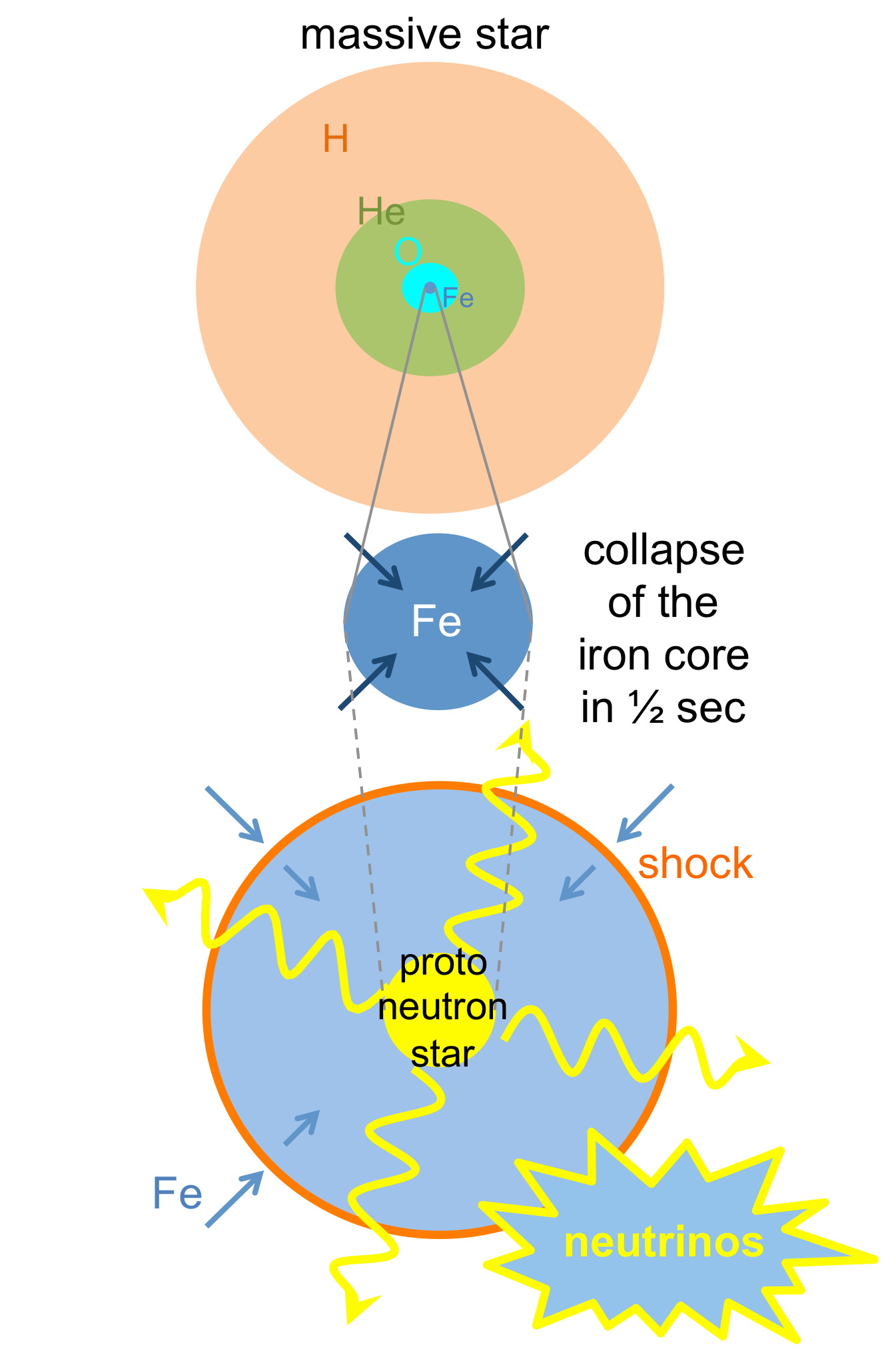
Figure 1.1: A visual representation of neutrino-driven explosion mechanism in CCSNe. The explosion mechanism relies on the absorption of neutrinos by the high-density post-shock gas. Figure credit: Foglizzo et al. (2015).

2) Core-collapse SNe (CCSNe): Massive stars having the ZAMS mass of $\geqslant$8 M_⊙ result into CCSNe as their terminating evolutionary stage (Gilmore, 2004; Woosley & Janka, 2005; Burrows & Vartanyan, 2021; Smartt, 2015; Foglizzo et al., 2015). Understanding the actual mechanism of the explosion for CCSNe is a long-standing problem. Theoretical studies spanning a period of more than half a century have been performed to understand these catastrophic phenomena, while much longer observational investigations are there. However, only recently has the mechanism of their explosion become a sharp focus. One of the most successful mechanisms in explaining the actual CCSNe process is the neutrino-driven explosion mechanism (Janka, 2012; Fryer & Kusenko, 2006; Burrows & Vartanyan, 2021; Janka, 2017). Massive stars evolve for a few million years (10 - 40 million years, depending upon initial mass) of age. During a massive star’s evolution, the star passes through successive burning phases of different elements. The massive star starts with burning Hydrogen in its core which continues for a major fraction of its entire evolution, and then it ignites Helium burning in the core. After that, successive burning of nuclear fusion reactions produces heavier nuclei, and the star develops an onion shell-like structure with heavier elements deeper in the star. During the last evolutionary stages, the massive star’s core primarily comprises inert Iron. The inert Iron-core of the massive star keeps growing until it reaches the Chandrasekhar mass limit of nearly 1.5 M_⊙, and becomes gravitationally unstable. Thus, after a few million years of evolution, the star’s dense core implodes as there is hardly any radiation pressure support to the self-gravity of the core. Within less than a second, the core obtains nearly nucleon densities while the stellar material surrounding the core also follows the infall (Figure 1.1). The central temperature is so high that it dissociates the Iron nuclei into protons and neutrons. Also, the densities are so high that the protons transform into neutrons and produce neutrinos. At this stage, an NS is born.

The infalling material encounters sudden and abrupt deceleration due to the stiff NS surface, which launches a shock wave. The shock propagates outwards until it stalls at a certain distance from the core. The stalled shock causes the wobble in the NS. This wobbling motion causes the asymmetric distribution of matter, modulating the flux of neutrinos leaking from the NS. This asymmetric wobbling motion of dense matter is capable of deforming the space-time fabric, which could be detected in the form of Gravitational-waves (GW) (Mezzacappa et al., 2020; Radice et al., 2019; Morozova et al., 2018; Andresen et al., 2017).

The wobbling shock starts rotating at the expense of the NS, which rotates in the opposite direction. The abundant densities are high enough to capture a few of the leaking neutrinos. The shock begins to expand in the direction where the matter below the shock catches the highest number of neutrinos. This is the decisive moment that marks the onset of the explosion. However, the shock will take some time to pass through the concentric envelopes of different elements and finally come out of the surface to mark an explosion. Meanwhile, the GWs and neutrinos have already propagated way ahead of the shock wave, and thus they are the first signals to come out of the surface of the collapsing star. After neutrino and GW signals, the shock break-out from the star’s surface provides the first observational electromagnetic signature of the collapse.

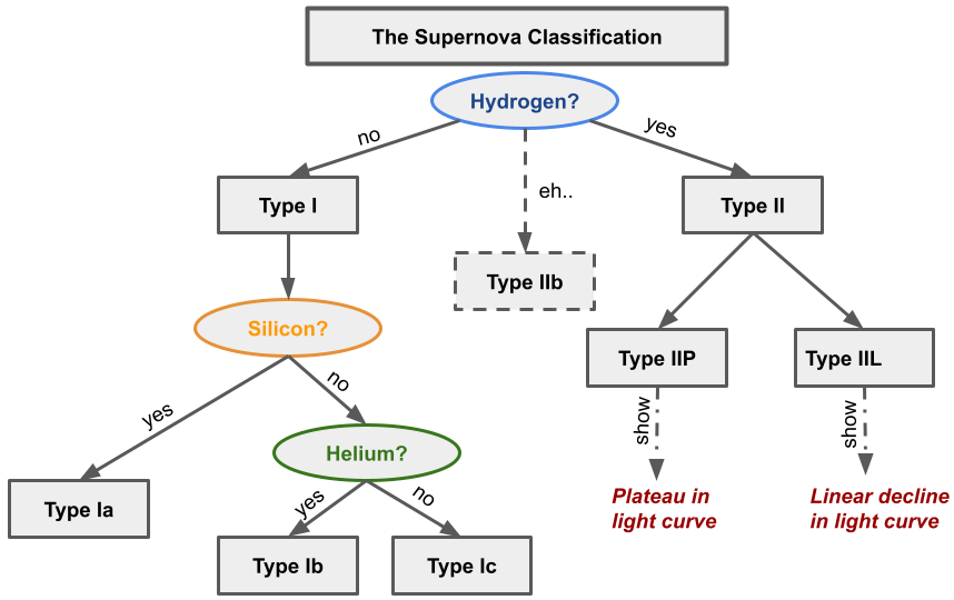
Figure 1.2: Classification of SNe primarily based on the observational features in their spectra and light curves using the results of (among others) Schlegel (1990), Filippenko (1997), and Gal-Yam (2017).

1.1.3 SN Classification on the basis of observational properties

Based on observational behaviour, SNe are primarily classified into two categories; First, H-rich Type II SNe, and Second, H-deficient Type I SNe. Figure 1.2 shows the various subclasses of Type II and Type I SNe. Figure 1.3 shows the classification of several types of SNe explicitly based on their spectroscopic observational features. Extensive reviews are provided in (among others) Filippenko (1997) and Gal-Yam (2017) on SNe classification. A brief of Type I and Type II SNe is provided below:

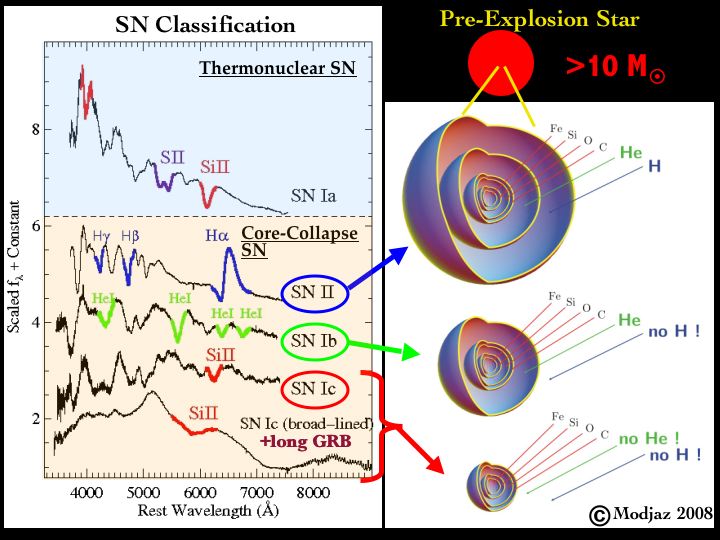
Figure 1.3: Spectra of several types of SNe (Left-hand panel). The thermonuclear SN Type Ia spectrum displays the strong features of S II and Si II and lacks any prominent H- or He-features. The Type II SN spectrum displays prominent features of hydrogen. Type Ib SN spectrum is well decorated with unambiguous He-features. Type Ic SNe spectra lack any prominent H- or He-features. Among CCSNe, the presence or absence of H- or He-features in the spectra depends upon the level of stripping their progenitor stars have gone through (Right-hand panel). The progenitors of Type II SNe suffer minimal stripping and retain most of their H-envelope; thus, they display prominent H-features in their spectra. Unlike Type II SNe, the progenitors of Type Ib SNe lose almost all of their H-envelopes through strong stellar winds or binary interaction; thus, their spectra lack any prominent H-feature but display strong He-features. Progenitors of Type Ic SNe suffer tremendous mass losses, and they cannot retain their outer H- as well as He-envelopes. Thus the spectra of Type Ic SNe are devoid of any prominent H- or He-features. Figure credit: Prof. Maryam Modjaz.

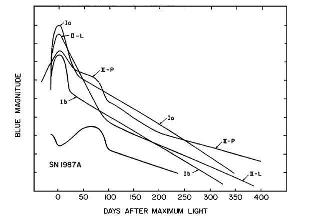
Figure 1.4: The light curves of various classes of SNe. The light curve of Type Ib SN represents the average of the light curves of Type Ib and Type Ic SNe. Figure credit: Filippenko (1997).

1) Type I SNe: These SNe lack prominent H-features in their spectra. Type I SNe display a wide range of spectroscopic features that are used to further sub-divide them into various categories; Type Ia SNe display strong Silicon features in their spectra, Type Ib SNe lack prominent Silicon features, but strong He-features dominate their spectra, Type Ic SNe neither display strong Silicon features nor prominent He-features. Rather the spectra are dominated by the prominent features of heavier elements/ions, including Calcium II near-IR triplet, Oxygen I $\lambda$ 7777 absorptions, and Ca II H&K absorption.

There exist a few more classes of interacting SNe among Type I. Type Ibn (Chugai, 2009; Pastorello et al., 2015; Maeda & Moriya, 2022; Moriya & Maeda, 2016; Shivvers et al., 2016; Metzger, 2022) and Type Icn (Metzger, 2022; Perley et al., 2022) are the rare classes of Type Ib and Type Ic SNe respectively, which show narrow emission interaction features of Carbon and/or Oxygen in their spectra. Type Ic-BL is another class of SNe belonging to Type Ic SNe displaying broad absorption features in the spectra (Valenti et al., 2008a; Mazzali et al., 2013; Chen et al., 2017a). Type Ic-BL SNe are thought to be associated with Long-GRBs (among many others, Mazzali et al., 2013). Intense investigations have been performed to understand the possible connections of GRBs and CCSNe (e.g.,Wang & Wheeler 1998; Bloom et al. 1999; Sokolov 2001; Cano et al. 2017; Hu et al. 2021; Kumar et al. 2022a).

2) Type II SNe: These SNe are identified by the strong presence of H-features in their spectra. They exhibit a wide range of spectroscopic and photometric behaviour. Type II SNe are further subdivided into two main categories, Type IIP and Type IIL, depending upon the shape of their light curves (Barbon et al., 1979; Doggett & Branch, 1985). Type IIP SNe display a plateau in their light curves, and Type IIL SNe show a linear decline in their light curves after maximum brightness (Figure 1.4).

Besides these two main subcategories of Type II SNe, a few more subclasses also exist; Type IIn SNe are the subclass of Type II SNe which display narrow emission lines in their spectra (Schlegel, 1990; van Dyk et al., 1996; Leonard et al., 2000; Moriya & Maeda, 2014; Smith, 2017; Ransome et al., 2021), Type IIb SNe initially display strong H-feature and in a few weeks their spectra are gradually dominated by He-features. Thus, Type IIb SNe are thought to be the link between H-deficient Type I and H-rich Type II SNe (Swartz et al., 1993). Beyond Type I and Type II SNe, there exists a class of superluminous SNe (SLSNe) having luminosities about 10–100 times greater than above mentioned canonical SNe (Nicholl, 2021).

1.2 Powering Mechanisms of Core-Collapse Supernovae

Several models have been proposed as the possible powering mechanism for CCSNe. In this section, we provide short explanations of different powering mechanisms.

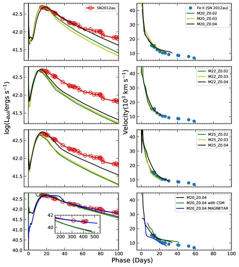
Figure 1.5: The results of the hydrodynamic modelling of SN 2012au, assuming the “Radioactive decay model”, “Circumstellar interaction model”, and the “Magnetar-driven model”. The “Magnetar-driven model” seems best to match the observed quasi-bolometric light curve of SN 2012au. Figure is adapted from Pandey et al. (2021).

1.2.1 Radioactive decay model

The radioactive decay of ⁵⁶Ni and ⁵⁶Co has been used to explain the observed light curves of SNe (Arnett, 1979, 1980, 1982; Mazzali et al., 1997; Elmhamdi et al., 2003; Stritzinger et al., 2006). In the process of the radioactive decay, ⁵⁶Ni decays to ⁵⁶Co which finally decays to stable ⁵⁶Fe (Nadyozhin, 1994). The deposition of gamma-rays resulting from the radioactive decay of ⁵⁶Ni and ⁵⁶Co are expected to thermalise in the homologously expanding SN ejecta and, after that, radiatively released to explain the light curves of several types of SNe including, Type Ia, Type Ib/c and Type II also (e.g., as found by (among many others), Pandey et al., 2003; Aryan et al., 2021b, 2022c; Vinkó et al., 2003; Zheng et al., 2022). The generalised mathematical expression governing the form of the output luminosity light curve is provided in Valenti et al. (2008a); Chatzopoulos et al. (2009, 2012).

1.2.2 Magnetar-driven model

The “Magnetar-driven model” has been very successful in explaining the light curves of SLSNe (Dessart et al., 2012b; Nicholl, 2021). In this model, the energy input by the spin-down of a magnetar sitting in the centre of the SN ejecta governs the output luminosity light curve of the corresponding SN (Ostriker & Gunn, 1971; Arnett & Fu, 1989; Maeda et al., 2007; Metzger et al., 2015; Kasen & Bildsten, 2010; Woosley, 2010). The mathematical expression governing the output luminosity light curve is given in Chatzopoulos et al. (2012) and Chatzopoulos et al. (2013). Beyond SLSNe, a few other Type I and Type II SNe have also been thought to be powered by a “Magnetar-driven” model. In Maeda et al. (2007), the authors have suggested the “Magnetar-driven” model as the possible powering mechanism for a peculiar Type Ib SN 2005bf. In another recent work by (Pandey et al., 2021), the photometric and spectroscopic properties combined with the hydrodynamic modelling of the exceptionally bright Type Ib SN 2012au indicated a ”Magnetar-driven model” for the powering of the light curves as shown in the Figure 1.5. Many studies demonstrate the “Magnetar-driven model” as the possible powering mechanism for several classes of CCSNe (e.g., Taddia et al., 2019; Sukhbold & Thompson, 2017; Chen et al., 2017a; Wang et al., 2016a).

1.2.3 Circumstellar interaction model

The “Circumstellar interaction model” is accepted as one of the dominant powering mechanisms for some SLSNe and other interacting SNe which display circumstellar interaction features. Several Type Ibn SNe have shown the interaction features of their ejecta with the circumstellar material (CSM) (e.g., among others, Karamehmetoglu et al., 2017a; Shivvers et al., 2017; Vallely et al., 2018; Sun et al., 2020). Unambiguous features of SN ejecta interacting with the CSM have also been identified in recent (among few other) Type Icn SN 2021csp (Perley et al., 2022), SN 2022ann (Davis et al., 2022), and SN 2021ckj (Nagao et al., 2023). In some cases, the SNe progenitors are surrounded by the dense CSM. The CSM is produced due to the continuous or intermittent pre-explosion mass losses from the progenitor. Upon the occurrence of the explosion, the SN ejecta may vigorously interact with the surrounding CSM (Chevalier, 1982; Chevalier & Fransson, 1994) resulting in the creation of a dual shock configuration; a forward shock moving in the CSM and a reverse shock that moves back into the SN ejecta. The kinetic energy from these shocks is transferred to the material, which is then released as radiation to power the light curves. The mathematical expression for the output luminosity light curve is given in Chatzopoulos et al. (2012) and Chatzopoulos et al. (2013).

1.2.4 Hybrid models

In some cases, the individual models mentioned above fail to reproduce the observed light curves of SNe, and one has to consider the contributions from more than one powering mechanism. Such a model, constituted out of two or more powering mechanisms to explain the light curves, is known as the “hybrid model” (please see, Chatzopoulos et al., 2012, 2013; Chatzopoulos & Tuminello, 2019; Moriya et al., 2018). Several combinations of two or more models are possible:

$\bullet$  Chatzopoulos et al. (2012, 2013) presented a “hybrid model” where the final luminosity light curve has the combined contribution from the “Radioactive decay model” and “Circumstellar interaction model”. Using this “hybrid model”, they attempted to explain the observed luminosity light curves of several SLSNe and Type IIn SNe.

$\bullet$  In another scenario, the authors of Chen et al. (2017b) and Inserra et al. (2017) have constituted the “hybrid model” by taking into account the collective contribution from “Magnetar-driven model” and the “Circumstellar interaction model” to explain the luminosity light curves of several SLSNe.

$\bullet$  A collective contribution from the “Radioactive decay model” and the “Magnetar-driven model” has been utilised to explain the light curves of several SLSNe (Bersten et al., 2016; Blanchard et al., 2019).

$\bullet$  To explain the light curve of a peculiar SLSN iPTF13ehe, the authors of Wang et al. (2016b) formulated a “hybrid model” by taking collective contributions from three mechanisms, namely, “Magnetar-driven model”, “Radioactive decay model”, and the “Circumstellar interaction model”.

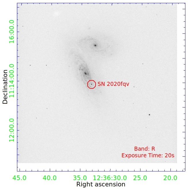
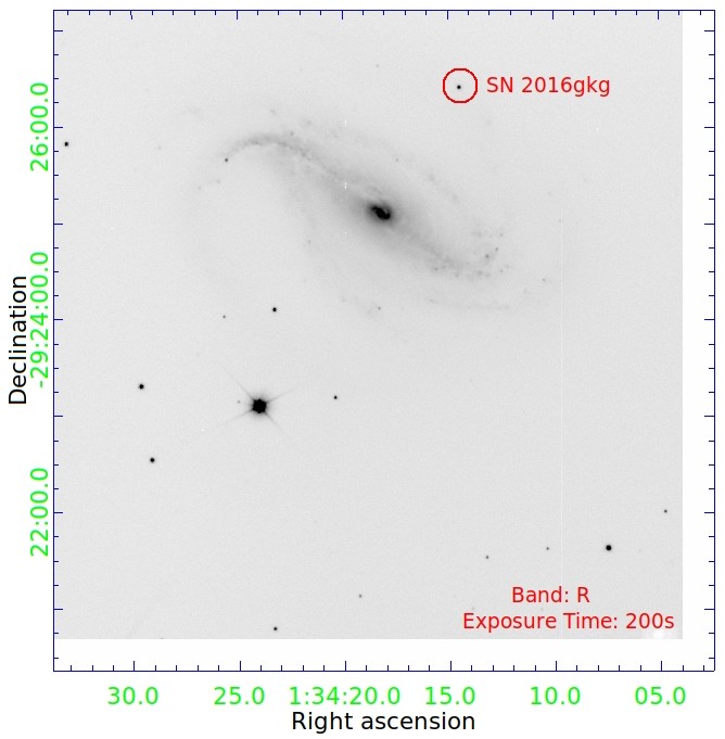
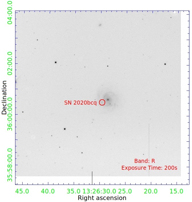
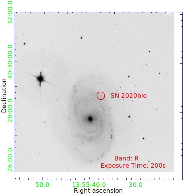
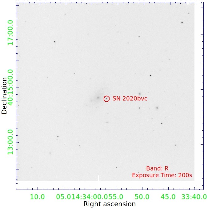
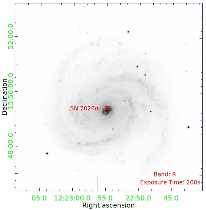
Figure 1.6: The first row shows the $R$-band images of SN 2020fqv and SN 2016gkg obtained using the 4K$\times$4K CCD imager (Pandey et al., 2018; Kumar et al., 2022b) mounted on the axial port of 3.6 m DOT (details of 3.6 m DOT are provided in Chapter 2). The remaining rows show the $R$-band images of SN 2020bcq, SN2020bio, SN2020bvc, and SN 2020oi using the 4K$\times$4K CCD imager.

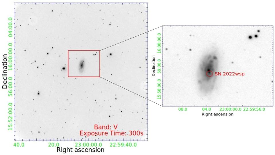
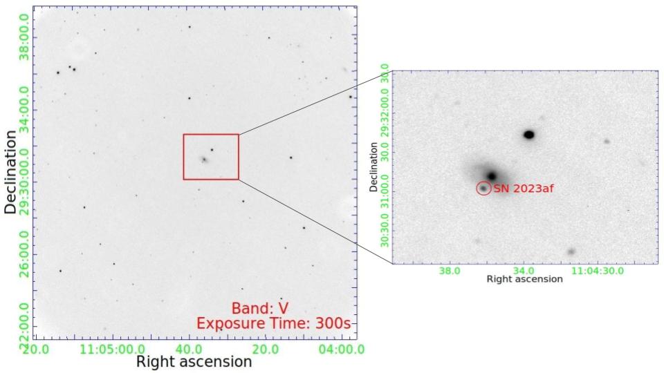
Figure 1.7: $V$-band images of SN 2020wsp and SN 2023af using the 2K$\times$2K CCD camera mounted at the axial port of 1.3 m DFOT (details of 1.3 m DFOT are provided in Chapter 2).

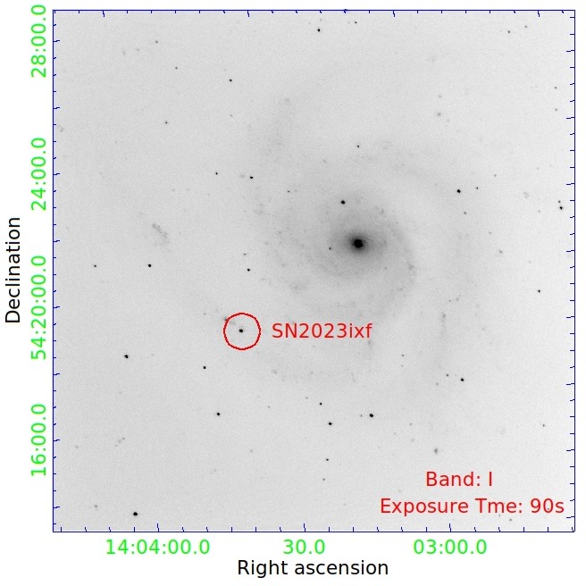
Figure 1.8: $I$-band images of SN 2023gfo and SN 2023ixf obtained using the 4K$\times$4K CCD camera mounted on the axial port of 1.04 m ST (details of 1.04 m ST are provided in Chapter 2).

1.3 Possible Progenitors and Ambient Environments of Core-Collapse Supernovae

Understanding the physical properties of possible progenitors of CCSNe and their ambient surroundings is the prime focus of current research among the SN community. Researchers and scientists primarily depend on observations and observation-complemented simulations to unveil the nature of the possible progenitors and the surrounding media. Figures 1.6, 1.7, and 1.8 show the diversity in host galaxies for the occurrence of several CCSNe.

1.3.1 Observational constraints on the progenitors and their surroundings

Knowledge of the possible progenitors of CCSNe is among the most fundamental aspects of understanding these catastrophic explosions. The most efficient way to investigate the likely progenitors of CCSNe and their physical properties is by directly detecting progenitors in high-resolution pre-explosion images from space- and ground-based telescopes. Such a detection would provide direct evidence of the mass, luminosity, temperature, and other physical properties of the underlying progenitor (e.g., Van Dyk et al., 2003b; Smartt et al., 2004; Li et al., 2006).

$\bullet$  Type IIP and Type IIL CCSNe

With the help of the direct detections of red supergiant (RSG) progenitors of Type IIP SNe and the most massive WD progenitors in pre-explosion images, a star requires to have a mass of at least 8$\pm$1 M_⊙ to finally terminate its life as a CCSN (Smartt, 2009). Although the direct detection of progenitors in the pre-explosion images is the most efficient way to understand them, only a few such detections have been obtained due to the uncertainties associated with the temporal and spatial position of the occurrence of an SN. It is impossible to predict the actual location and timing of the occurrence of an SN. As per the review provided in (Smartt, 2015), there are only 18 detections of precursor objects and 27 upper limits in archival images from the ground- and space-based telescopes. Among these, most of the detections of progenitor stars are for Type IIP, IIL, or IIb SNe. Additionally, only one detection for Type Ib SN progenitor is available. Beyond these detections, 14 upper limits are also there for Type Ibc CCSNe.

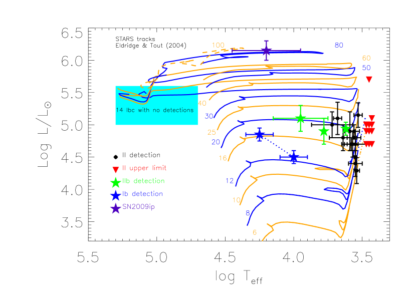
Figure 1.9: The positions of all the detected Type II and Type Ibc SNe progenitors. Upper limits to the detections are also shown. Two positions connected by dashed lines correspond to two progenitors presented by Bersten et al. (2014) and Eldridge et al. (2015). There is a debate over SN 2009ip to be a genuine CCSN, although it had a very massive progenitor (Smith et al., 2010; Foley et al., 2011; Smith, 2011; Mauerhan et al., 2013; Prieto et al., 2013; Fraser et al., 2013). The stellar evolutionary tracks in this figure are from Eldridge & Tout (2004). Figure credit: Smartt (2015).

In the volume-limited calculations, the frequency of the occurrence of Type IIP SNe is highest among several Types of SNe (Smartt et al., 2009; Li et al., 2007; Prieto et al., 2008; Cappellaro et al., 1999); therefore, Type IIP SNe progenitor population is currently the best understood observationally with the help of available direct detections and upper limits. A few Type IIP SNe having clear detections of their progenitors are discussed here. The first example is SN 2003gd from a nearby galaxy, M74. Through the archival images of M74 imaged some 6–9 months before the explosion utilising the Hubble Space Telescope and the Gemini North telescope, researchers could identify the possible progenitor of SN 2003gd (Van Dyk et al., 2003b). The identified progenitor has a $V$-band magnitude of 25.8$\pm$0.15 (Smartt, 2009). Further investigations by (Smartt et al., 2004) reveal that the possible progenitor of SN 2003gd is an RSG. The initial mass of the identified progenitor likely lies in the range of 8${}^{+4}_{-2}$ M_⊙. The metallicity at the SN 2003gd explosion site was probably near solar (Smartt, 2009).

The following Type IIP SN with progenitor detection in pre-explosion images is SN 2005cs, which occurred in the whirlpool galaxy, M51. The investigations of HST images by Maund et al. (2005) and Li et al. (2006) constrain the progenitor to be an RSG again having a mass of 8$\pm$2 M_⊙. SN 2008bk is another Type IIP SN with its progenitor detection in pre-explosion images having a significant confidence level. Mattila et al. (2008) could constrain the progenitor to be an RSG with a mass of 8.5$\pm$1.0 M_⊙. The metallicity of the host galaxy at the SN 2008bk explosion site lies between the metallicity of Small Magellanic Cloud (SMC) and Large Magellanic Cloud (LMC) (Smartt, 2009).

Unlike the vast majority of CCSNe in the local Universe exploding in the star-forming regions (Van Dyk et al., 2003a), SN 2004dj and SN 2004am are the examples of CCSNe originating in star clusters (Smartt et al., 2009). The SN 2004dj occurred in a well-studied star cluster Sandage 96 (Maíz-Apellániz et al., 2004). The authors of Maíz-Apellániz et al. (2004) estimated the age of the cluster to be nearly 14 Myr and the corresponding initial mass of the identified progenitor to be around 15 M_⊙. In another work, Wang et al. (2005) estimated an initial progenitor mass of 12 M_⊙. A main-sequence mass in the range of 12–20 M_⊙ is inferred for the identified progenitor by the calculations of Vinkó et al. (2009). Like SN 2004dj, the SN 2004am exploded in another super star cluster L in M82. The identified progenitor is estimated to have an initial mass of 12${}^{+7}_{-3}$ M_⊙ (Smartt, 2009) derived from the star cluster age of 18${}^{+17}_{-8}$ Myr (Lançon et al., 2008). A list of Type II CCSNe with secure progenitor detections and upper limits on detection are given in Smartt (2015) in Table 1 and Table 2 there.

There are detections of progenitors for three more Type IIP SNe, namely, SN 1999ev, SN 2004A, and SN 2004et, but the significance level of their detections could be better. Following Maund & Smartt (2005), if the detected progenitor for SN 1999ev is an RSG then the corresponding mass of the progenitor is around 15–18 M_⊙. For SN 2004A, Hendry et al. (2006) suggests the initial mass of an RSG progenitor to be 9${}^{+3}_{-2}$ M_⊙. Further, a yellow supergiant star of initial mass around 15 M_⊙ is claimed to be the possible progenitor of SN 2004et by Li et al. (2005), but later Smartt et al. (2009) questioned its identification as the detected object was visible at the same luminosity even after around four years later since the SN explosion. Finally, Smartt et al. (2009) suggested a supergiant star having an initial mass of 9${}^{+5}_{-1}$ M_⊙ as the detected progenitor of SN 2004et. A few more detections of Type IIP SNe progenitors were claimed in pre-explosion images, but those detections are debatable (please see, Li et al., 2007; Leonard et al., 2008; Smartt et al., 2009).

Following Smartt et al. (2009), the occurrence frequency of Type IIL SNe is lowest. These SNe have very short or no plateau in their light curves, probably due to low-mass H-envelope not being capable of sustaining a longer duration of recombination (Smartt, 2009). A Type IIL SN progenitor could lose mass through strong stellar winds or binary interaction, resulting in a corresponding low-mass H-envelope. A higher mass progenitor than the Type IIP SNe progenitor is expected if the mass loss occurs through stellar winds (Smartt, 2009). There are two incidences of progenitor detections for Type IIL SNe as tabulated by Smartt (2015). The authors of Elias-Rosa et al. (2011) could constrain the properties of the progenitor of SN 2009hd using the pre-explosion HST images. The estimated magnitude and colour limits indicate a luminous RSG star with the possibility that the progenitor star could have been rather yellow than red. The investigations by Fraser et al. (2010) and Elias-Rosa et al. (2010) utilising the archival HST images claim the progenitor detection for SN 2009kr. The authors of Fraser et al. (2010) claim a yellow supergiant (YSG) star having a mass of 15${}^{+5}_{-4}$ M_⊙ while the estimated initial mass of the YSG progenitor by Elias-Rosa et al. (2010) is 18–24 M_⊙.

Last but not least, the recent discovery of one of the nearest H-rich Type II SN 2023ixf in the pinwheel galaxy (M101) has opened new avenues to understanding the possible progenitors of H-rich CCSNe. The analysis by Kilpatrick et al. (2023) indicate towards an RSG progenitor of 11 M_⊙ for SN 2023ixf.

$\bullet$  Type IIb CCSNe

Type IIb SNe begin by displaying unambiguous signatures of H-features in their spectra and later evolve to exhibit strong He-features along with weaker H-features (Filippenko, 1997). For Type IIb SNe also, a few cases have been reported (Smartt, 2015) where the progenitor stars are detected in pre-explosion images:

(a) Crockett et al. (2008) identified the progenitor star for SN 2008ax in the pre-explosion images from HST archival images. Based on their detections, they proposed two possible scenarios for the progenitor; First, a single massive star that has stripped off most of its H-envelope utilising radiatively driven mass-loss mechanisms. Finally, the exploding progenitor is an He-rich Wolf-Rayet (WR) star retaining only a tenuous H-envelope. Second, an interacting binary progenitor system where the mass loss primarily due to binary interaction is responsible for the production of stripped progenitor.

(b) Maund et al. (2011) and Van Dyk et al. (2011) have claimed to identify the progenitor of SN 2011dh in pre-explosion archival images obtained through HST. By comparing the position of the detected progenitor on the HR diagram with several stellar evolution tracks, Maund et al. (2011) propose a single YSG star at the end of core Carbon-burning having an initial mass of 13$\pm$3 M_⊙ as the possible progenitor for SN 2011dh. While comparing the position of the detected object on HR diagram with several stellar evolution tracks, Van Dyk et al. (2011) propose an initial mass in the range of 17–19 M_⊙.

(c) SN 2013df is another Type IIb SN with its progenitor detected in the pre-explosion images with a significant confidence level. Van Dyk et al. (2014) have claimed to confirm the detection of progenitor star of SN 2013df in pre-explosion archival images from HST obtained around 14 years before the actual SN explosion. The identified progenitor is a YSG star with an initial mass of 13–17 M_⊙. The positions of detected progenitors of Type II CCSNe on the HR diagram are shown in Figure 1.9. The upper limits are also shown there.

$\bullet$  Type Ibc CCSNe

Following Smartt (2015), only one case of progenitor identification has been reported for a Type Ibc SN. For the site of SN iPTF13bvn, the HST pre-explosion images indicate the presence of a blue star. But, Cao et al. (2013) indicated that the detected progenitor was not within the 1$\sigma$ error circle in their alignment of a ground-based image having significantly high resolution. Still, the detection could not be strongly rejected as the detection was well within 3$\sigma$. Later, utilising the alignment with HST images, Eldridge et al. (2015) supported the argument mentioned above and suggested it to be the first-ever detection of a progenitor for Type Ibc SN (particularly Type Ib). Further analysis by Cao et al. (2013) and Groh et al. (2013) proposed that the identified progenitor probably was a single massive with an initial mass of around 30 M_⊙ that later evolved into a WN star. Alternatively, binary progenitor scenarios with initial masses of 20 + 19 M_⊙ or 10 + 8 M_⊙ were also proposed (Bersten et al., 2014; Eldridge et al., 2015). Figure 1.9 shows the corresponding positions of proposed progenitors.

1.3.2 Simulation-based investigations on the possible progenitors and surroundings

As mentioned in the previous subsection, direct detection of progenitors in pre-explosion images is the most successful method to constrain their physical properties and the ambient environment around them. With the help of observationally derived parameters, reliable progenitor models can be built for several classes of SNe. With the help of many state-of-the-art simulation tools, those models can be evolved up to their late evolutionary stages. Such simulation-based studies are essential to explain and understand the physics behind observed phenomena.

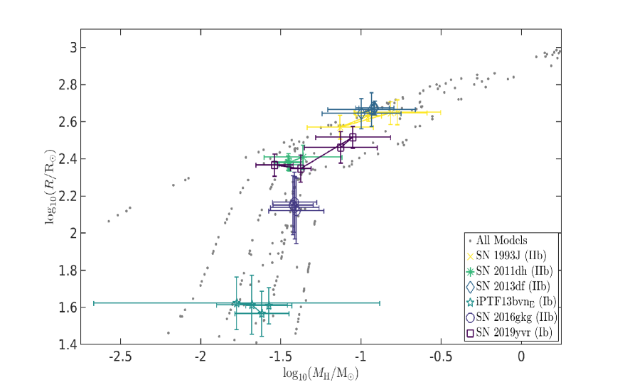
Figure 1.10: Mean hydrogen mass as a function of mean progenitor stellar radius along with their standard deviation. Figure credit: Gilkis & Arcavi (2022).

Utilising the 1-dimensional hydrodynamic simulations, Fuller (2017) attempts to explain the pre-explosion outbursts activities in RSG progenitors via wave heating. The author also finds that the wave heating in massive stars could explain some flash-ionised SNe and a few diversity observed in Type IIP and IIL CCSNe. As the surface abundances play an essential role in decorating the spectrum with the features of several elements/ions, authors of Davies & Dessart (2019) attempt to investigate the surface abundances of RSG stars utilising 1-dimensional simulations. In another work, Fuller & Ro (2018) examine the effect of wave heating in massive H-poor stars serving as the progenitors of Type IIb/Ib CCSNe. They find that only a subset of these progenitors is expected to experience pre-explosion outbursts due to wave heating. Type Ib/IIb CCSNe are stripped SNe that arise from progenitors that have retained very little to no hydrogen at the time of their explosions. However, the uncertainties associated with determining the extinction and distance of the underlying CCSN affect the correct estimation of the amount of hydrogen retained by the progenitor at the pre-explosion stage. While studying the progenitor channels for Type IIb CCSNe, Gilkis & Arcavi (2022) find that the post-interaction mass-loss rate plays a vital role on the amount of hydrogen retained in the envelope by the underlying progenitor at the time of the explosion. Figure 1.10 shows the mean of the amount of hydrogen as a function of the mean stellar progenitor radius for all the models in their study, including several Type Ib/IIb CCSNe. Earlier, the authors of Sravan et al. (2019) also explored the impact of single- vs binary-progenitor systems for Type IIb CCSNe. They found that both the progenitor systems contributed to roughly the same number of Type IIb SNe at solar metallicity. However, at lower metallicities, the binary-progenitor channel dominated over single. At the time of investigating the evolution of He-rich progenitor stars through 1-dimensional simulations, Kleiser et al. (2018) find that the amount of ⁵⁶Ni synthesised plays a key role in separating rapidly fading Type I SNe with normal Type Ibc SNe.

1-dimensional stellar evolutions are helpful in investigating the pre-explosion activities, while post-explosion properties, including bolometric or multi-band light curves, are explored with the help of synthetic explosions of stellar models on the verge of core collapse. Utilising several state-of-the-art 1-dimensional stellar evolution codes, artificial models are computed based on the observational behaviour of the underlying SN. The stellar-model is evolved through various stages of its life until it reached the onset of core collapse. Further, the model on the stage of the beginning of core collapse is exploded synthetically to produce simulated bolometric light curves, multi-band light curves, and many other photospheric properties. These simulated properties are compared with actual observations. Such a comparison of simulated results with actual results further helps to put important constraints on the physical properties of the underlying SN progenitor.

Exploring the lack of consensus over the progenitor masses of Type IIP CCSNe, Utrobin (2007) could put important constraints over pre-explosion characteristics of the exploding star and several SN properties with the help of hydrodynamic and time-dependent atmosphere models. They estimate that the exploding progenitor of the Type IIP SN 1999em had a pre-SN radius of 500$\pm$200 R_⊙. It ejected an enormous amount of matter as indicated by an ejecta mass of 19.0$\pm$1.2 M_⊙. The estimated explosion energy and the amount of ⁵⁶Ni synthesised were (1.3$\pm$0.1)$\times$10⁵¹ erg and 0.036$\pm$0.009 M_⊙, respectively. They attempted to derive approximate connections between basic physical and observationally-obtained parameters and concluded that the hydrodynamic and atmospheric models needed more consistency. They also concluded that the hydrogen recombination event in all the Type IIP SNe is time-dependent at their photospheric epochs.

The hydrodynamic simulations are essential to investigate the shortcomings of the proposed model and the effect of multi-dimensions. In Utrobin & Chugai (2009), the authors find out that the inferred progenitor mass of SN 2004et through hydrodynamic simulations is much higher than obtained through pre-explosion images earlier. The mismatch between the progenitor mass estimates through pre-explosion images and hydrodynamic simulations was speculated to be the multi-dimensional effect.

With time, attempts to incorporate the improvements suggested in previous studies to make more realistic models were made. Bersten et al. (2011) presented bolometric light curves of Type IIP SNe obtained using a 1-dimensional Lagrangian hydrodynamic code that utilises flux-limited radiation diffusion approximation (Levermore & Pomraning, 1981). Utilising their code, the authors obtained remarkable agreement between the observationally-obtained parameters and simulated results for SN 1999em. In another work by Dall’Ora et al. (2014), the authors presented hydrodynamic modelling of a Type IIP SN 2012aw utilising accurate spectroscopic and photospheric observations. They estimated that the underlying progenitor had an envelope mass of around 20 M_⊙, progenitor radius of $\sim$430 R_⊙, explosion energy of $\sim$1.5$\times$10⁵¹ erg and initial ⁵⁶Ni mass of around 0.06 M_⊙. In Pumo et al. (2017), the authors attempted to improve the current understanding of the possible progenitors of under luminous CCSNe Type IIP through radiation hydrodynamics modelling. Their investigations indicated that the low luminosity Type IIP CCSNe originated from relatively lower mass progenitors, and the catastrophic explosions were less energetic than intermediate luminosity Type IIP CCSNe. In a recent work, the authors of Martinez et al. (2020) attempted to estimate the physical parameters of Type II SNe. Using statistical interference techniques, they simultaneously fitted the bolometric light curve and the corresponding photospheric velocity evolution to hydrodynamic models. They found that the progenitor mass constraints were in very well agreement with the progenitor mass limits derived through pre-explosion images. Finally, they displayed that hydrodynamic modelling of progenitors can be used to put robust constraints over the physical properties of Type II SNe. In relatively recent work, Martinez et al. (2022) performed a similar study and estimated the physical parameter distribution of an ensemble containing 53 Type II SNe through hydrodynamic modelling. Their analysis indicated a range of physical parameters for Type II SNe considered in their study with ejecta mass lying in the range of (7.9–14.8) M_⊙, explosion energies lying between 0.15$\times$10⁵¹ erg and 1.40$\times$10⁵¹ erg. Additionally, the inferred ⁵⁶Ni mass for the SNe in the sample lies in the range of (0.006–0.069) M_⊙. A few studies have also attempted to perform the hydrodynamic simulations of Type IIn (Li & Morozova, 2022; Kuriyama & Shigeyama, 2020; Dessart et al., 2015) and Type IIL SNe (Bostroem et al., 2019; Sukhbold et al., 2016) also.

Compared to other Type CCSNe, the literature is significantly populated with hydrodynamic modelling of Type IIP SNe. Specifically, the hydrodynamic modelling of Type IIP SNe is relatively more straightforward than other CCSNe since the former occurs in an environment with very low density (Baron et al., 2000; Chevalier et al., 2006). Additionally, the progenitors of Type IIP SNe have extended and nearly spherically symmetric outer H-envelopes, which suppress any inhomogeneities arising from diverse explosions (Leonard & Filippenko, 2005). Unlike Type IIP SNe, stripped-envelope CCSNe of Type Ibc and Type IIb have relatively compact progenitors. The complicated stages of envelope burning in them make it very difficult to perform their stellar evolution and then compute the hydrodynamic simulations of their explosions. Only a handful of such studies have been performed for stripped-envelope CCSNe.

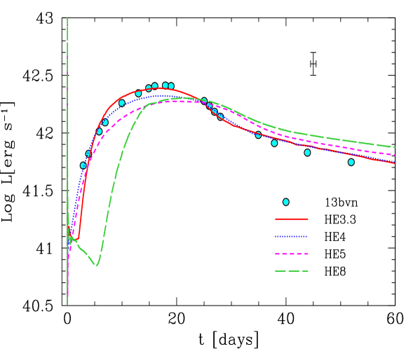
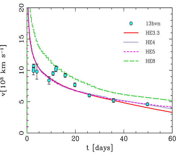
Figure 1.11: Hydrodynamic modelling outcomes for iPTF13bvn. The model names correspond to the progenitor star’s pre-SN mass (e.g., for HE3.3, the pre-SN mass is 3.3,M_⊙). A comparison was made between the model bolometric light curves (displayed in the left panel) and the evolution of photospheric velocity (shown in the right panel) with the actual observations. The model featuring a 3.3,M_⊙ pre-SN mass exhibited the closest agreement with the observed data. Figure credit: Bersten et al. (2014).

After confirming the location of the progenitor candidate of the SN iPTF13bvn, the authors of Fremling et al. (2014) perform hydrodynamic modelling of the bolometric light curve to constrain the amount of ⁵⁶Ni synthesised and the ejecta mass. They find that iPTF13bvn synthesised an amount 0.05 M_⊙ of ⁵⁶Ni and the corresponding ejecta mass was 1.9 M_⊙. They also find that the bolometric light curve does not follow the single massive WR-star possible progenitor scenario as predicted in earlier studies. In another work by Bersten et al. (2014) also, the authors predict a binary interacting progenitor system for iPTF13bvn and perform the evolutionary calculations. Their models could explain the light curve shape (left panel in Figure 1.11), photospheric velocity evolution (right panel in Figure 1.11), the absence of Hydrogen, and also the pre-SN photometry. The results from their hydrodynamic modelling suggest that the pre-SN stage mass of the progenitor was $\approx$ 3.3 M_⊙ and the initial mass of the progenitor could not be larger than $\approx$ 8 M_⊙. Later, Eldridge et al. (2015) also incorporated a set of several binary progenitor models to put constraints over the probable binary system of iPTF13bvn. According to their investigations, the two companions in the binary progenitor system of iPTF13bvn would have masses of 10 M_⊙ and 20 M_⊙.

A few studies have presented the stellar evolution of the possible progenitors of Type IIb SNe also and have performed the hydrodynamic simulations of their explosions. Bersten et al. (2012) utilised a set of several hydrodynamic models to explore the properties of underlying progenitor. According to their estimates, SN 2011dh probably exploded from a large progenitor star with a radius of $\sim$ 200 R_⊙. The exploding star probably had an He-core of 3–4 M_⊙ and retained a thin H-envelope at the pre-SN stage. The corresponding initial mass estimate for the progenitor was in the range of 12–15 M_⊙. They estimated an ejecta mass of around 2 M_⊙, explosion energy of (6–10)$\times$10⁵⁰ erg, and about 0.06 M_⊙ of ⁵⁶Ni synthesised. The small initial progenitor mass constraints ruled out the possibility of a single-star evolution scenario as the progenitor of SN 2011dh.

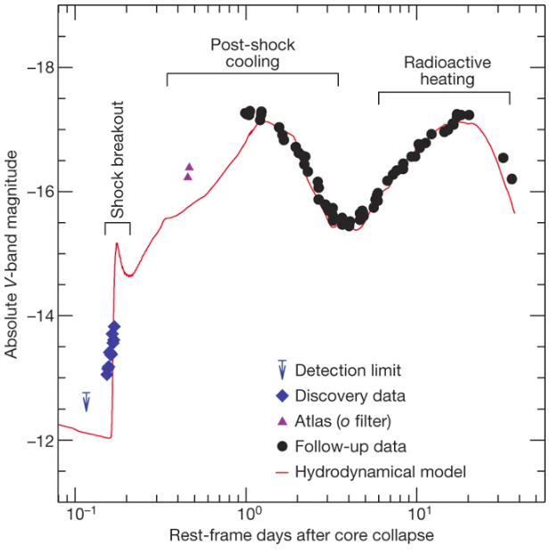
Figure 1.12: The outcome of hydrodynamic modelling for SN 2016gkg successfully replicated its distinct phases: the initial shock-breakout phase, the subsequent peak during shock cooling, and the later peak arising from the radioactive decay of ⁵⁶Ni and ⁵⁶Co. Figure credit: Bersten et al. (2018).

The authors of Morales-Garoffolo et al. (2015) performed hydrodynamic simulations to model the pseudo-bolometric light curve and the photospheric velocity evolution of SN 2011fu. Their analysis indicates that the SN 2011fu exploded from a progenitor star having an initial mass of 13–18 M_⊙. Further, they found that the exploding star released a kinetic energy of 1.3$\times$10⁵¹ erg, and the amount of ⁵⁶Ni synthesised was 0.15 M_⊙.

The serendipitous identification of Type IIb SN 2016gkg in its extremely early stages served the purpose of performing unprecedented explorations on CCSNe. It revealed a rapid brightening in optical wavelengths of nearly 40 magnitudes per day during the very early phases of detection (Bersten et al., 2018). In Bersten et al. (2018), authors performed the hydrodynamic modelling of the explosion to account for the different phases of the evolving SN (the preferred model is shown in Figure 1.12). The preferred model in their work had an initial mass of 18 M_⊙ with solar abundances and a pre-SN mass of 5 M_⊙. The object in the preferred model had an H-rich envelope of radius 320 R_⊙ and the corresponding mass of the H-rich envelope was found to be 0.01 M_⊙.

1.4 Core-Collapse Supernovae from Population III stars

The birth of the very first generation of stars, known as the Population III (Pop III) stars, marked the end of cosmic dark ages as they were responsible for generating fundamental modifications to the early Universe through the production of ionizing photons and enrichment with heavy elements (Bromm, 2013). There are multiple investigations which indicate that the Pop III stars were intrinsically very massive (e.g., Carr et al., 1984; McDowell, 1986); however, a few studies have also investigated the possibilities of the existence of relatively low mass Pop III stars (e.g., Turk et al., 2009; Ishiyama et al., 2016; Wollenberg et al., 2020). Pop III stars have been postulated to have multiple cosmological consequences, including production of 3 K microwave background radiation (Rees, 1978), chemical enrichment (e.g., Kirihara et al., 2020), dust formation (e.g., Todini & Ferrara, 2001), cosmic reionization (e.g., Hogan, 1979), etc.

Due to their cosmological importance, Pop III stars are fascinating objects of research despite their non-observance to date. It has been established through numerical studies that sufficiently large, very massive stars directly collapse to form BHs, while there is a tendency to explode in smaller ones (Carr et al., 1984). The authors of Nomoto et al. (2004) mentions that massive stars with masses greater than around 20 – 25 M_⊙ form BHs to terminate their life. The stars with non-rotating BHs collapse to result in faint SNe, while the rotating BH case can produce highly energetic SNe popularly known as hypernovae (HNe) (Nomoto et al., 2004). Several studies are there to understand the evolution of massive Pop III stars. The authors of Marigo et al. (2003) investigate the evolution of massive Pop III stars in the mass range of [120 – 1000] M_⊙ and the consequences of mass losses. The evolutions of two single Pop III stars and one binary system of Pop III stars are studied in Lawlor et al. (2008). Based on the sample of available models in their work, they find that Pop III SNe have a fainter peak but long plateau phase in their light curves. In another work, Heger & Woosley (2010) have studied the evolution and explosion of Pop III stars in the mass range of [10–100] M_⊙. Their studies indicate that most of the non-rotating Pop III stars become blue supergiants (BSGs) at the end of their life to result in SNe resembling the light curve of SN 1987A finally; however, a few are found to become RSGs, and the light curves of resulting SNe resemble Type IIP SNe.

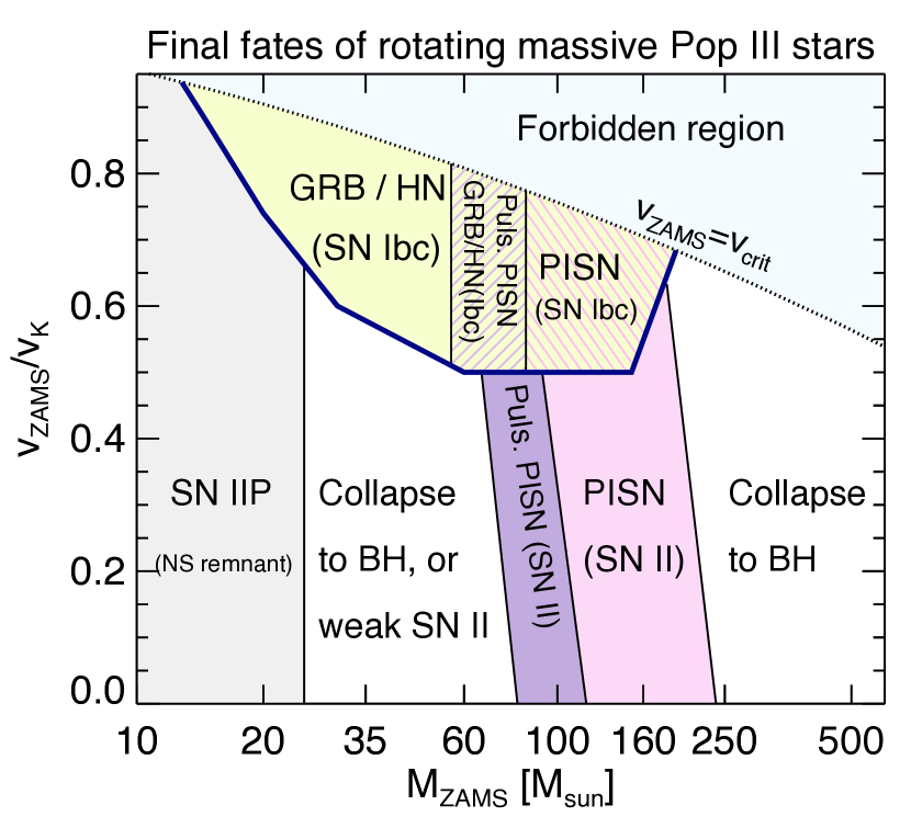
Figure 1.13: Phase diagram depicting the terminating fates of massive Pop III stars. In the regions above the dotted line, surface rotational velocity surpasses the critical threshold, thus that is the forbidden region. Further, the chemically homogeneous evolution is effective in the mass range of around [13 – 190] M_⊙, indicated by the thick (blue) solid line. Figure credit: Yoon et al. (2012).

In Yoon et al. (2012), the authors investigated the effect of including rotation and magnetic fields on the evolution of massive Pop III stars in the mass grid covering a range of [10–1000] M_⊙. In the considered mass grid, the authors identified the effect of chemically homogeneous evolution for a limited mass and rotational velocity range. They find that the effect of chemically homogeneous mixing is not seen beyond a ZAMS mass of 190 M_⊙. Depending upon the rotational velocity and ZAMS mass, the final fates of the Pop III stars could span a wide range of transient events, including several classes of SNe, GRBs, HNe, PISNs, PPISNs, or collapse directly to form a BH. A corresponding phase diagram in the plane of ZAMS mass and rotational velocity at ZAMS is depicted in Figure 1.13. To determine the signatures of detection and identification of Pop III SNe, the authors of Tolstov et al. (2016) performed a multicolour light curve simulation of several Pop III CCSN model resulting from Pop III stars having mass in the range of [25 – 100] M_⊙. They find that the multicolour light curves could be significantly helpful in identifying the Pop III SNe through current and future transient surveys. For the past few decades, researchers have been trying hard to find observational signatures of Pop III SNe (e.g., Frost et al., 2009; Ishigaki et al., 2014; Moriya et al., 2019; Yoshii et al., 2022; Padmanabhan & Loeb, 2022; Ezzeddine et al., 2019; Matsumoto et al., 2016).

1.5 Thesis Layout

There are seven Chapters in this thesis. The research work under the presented thesis investigates the photometric and spectroscopic behaviour of a number of CCSNe of different types. An attempt to understand the underlying progenitor, possible powering mechanisms, and surrounding environments has been made by utilising the photometric and spectroscopic data from several national and international telescopes. The research work under this thesis also uses several state-of-the-art simulation tools to perform the 1-dimensional stellar evolution of the possible progenitors and simulate their explosions to replicate the actual SN explosions. Part of the research work in this thesis contains observational data-based research work complemented by simulation-based analysis for a subset of new CCSNe. In contrast, some parts involve simulation-based investigations of the evolution and explosion of proposed SN models from the literature. A brief overview of each Chapter is provided below:

Chapter 1: In this Chapter, we present a comprehensive perspective on the existing knowledge within the research field, focusing on the powering mechanisms, potential progenitors, and surrounding environments of catastrophic CCSNe. This introductory Chapter also provides an overview of SNe’s historical observations, current progress in the field, and persisting issues of active research to set the context of present research work.

Chapter 2: Data from several telescopes and numerous state-of-the-art simulation tools are required to address issues outlined in Chapter 1, concerning the possible progenitors, powering mechanisms, and ambient media around CCSNe. The details of observations, data reduction, and modelling tools employed to carry out the research work in the presented thesis are discussed in Chapter 2. We also provide the details of several national and international telescopes utilised to obtain the photometric and spectroscopic data.

Chapter 3: Understanding the possible progenitors of CCSNe is one of the most fundamental tasks in understanding these catastrophic explosions. Therefore, within Chapter 3, we aim to illuminate the origins of the underlying progenitors of two Type Ib CCSNe, SN 2015ap and SN 2016bau, by performing their photometric and spectroscopic analyses. Our analyses show that SN 2015ap has intermediate luminosity among a subset of similar SNe, while SN 2016bau suffers very high host galaxy extinction and appears relatively less luminous. With the help of synergistic investigations utilising optical data from several telescopes and state-of-the-art simulation tools, we find that SN 2015ap originated from a 12 M_⊙ ZAMS progenitor, while a slightly less massive ZAMS progenitor is expected for SN 2016bau. Both the SNe seem to originate at the solar metallicity abundance sites of their corresponding host galaxies. The results of this work are published in Aryan et al. (2021b) and Aryan et al. (2022a).

Chapter 4: Having discussed the properties of two H-deficient Type Ib SNe in Chapter 3, we perform the photometric and spectroscopic investigations of a Type IIb SN 2016iyc in this Chapter. Type IIb SNe are thought to be the interconnecting link between H-rich and H-deficient CCSNe. Thus, the strategic investigations of Type IIb SNe are essential to enlighten the possible connections between H-rich and H-deficient CCSNe. The progenitors of Type Ib/IIb CCSNe retain very little to no hydrogen at the time of their explosions. However, the correct estimation of the amount of hydrogen retained before explosion by the underlying CCSN progenitor is subjected to contamination by the uncertainties associated with determining the extinction and distance of the CCSN.

In this Chapter, we investigate the photometric and spectroscopic analysis of a Type IIb SN 2016iyc. Our studies indicate SN 2016iyc lies towards the fainter luminosity regions among a subset of similar types of SNe. Based on the photometric and spectroscopic behaviours, the stellar evolution of progenitor models with ZAMS mass in the range of (9–14) M_⊙ is performed. Finally, the comparison of simulation-produced light curves and photospheric velocity evolution indicate that SN 2016iyc probably originated from a star having ZAMS mass in the range of (12–13) M_⊙. Our analysis also suggests that the host galaxy metallicity at the site of the occurrence of SN 2016iyc is probably solar. This Chapter also presents the hydrodynamic modelling of two other Type IIb SNe, SN 2011fu and SN 2016gkg. Based on the analysis conducted in this Chapter, we also find that Type IIb SNe progenitors preserve some trace amount of hydrogen at their pre-SN phase. This hydrogen mass appears to fall somewhere between the amount retained by the progenitors of H-rich and H-deficient SNe during their pre-SN stages. The results are published in Aryan et al. (2022c).

Chapter 5: After discussing the properties of H-deficient SNe in Chapter 3, the behaviour of a Type IIb SN retaining an intermediate amount of H-envelope in Chapter 4, this Chapter discusses H-rich and H-deficient SNe together that originate from progenitors each starting with a mass of 25 M_⊙ at ZAMS and zero metallicity. CCSNe from massive Pop III stars are postulated to have had an enormous impact on the early Universe. The SNe from Pop III stars were responsible for the initial enrichment of the early Universe with heavy elements, and they also played a pivotal role in cosmic reionization. This Chapter comprises pure simulation-based results of the stellar evolution of a 25 M_⊙ ZAMS progenitor with zero metallicity and investigates the effects of rotation on the resulting SNe. The hydrodynamic simulation of the resulting CCSNe is also presented in this Chapter. The rapidly rotating models display violent mass losses after their main-sequence phases compared to non-rotating and slowly rotating models. Further, the light curves of rapidly rotating models resemble Type Ib/c SNe, while slowly rotating models mimic the light curves of Type IIP SNe. These results are published in Aryan et al. (2023).

Chapter 6: Chapter 3, Chapter 4, and Chapter 5 discuss the properties of canonical CCSNe arising from progenitors having ZAMS masses of 25 M_⊙ or less. However, in this Chapter, we present the pure simulation-based results of the stellar evolution of a 100 M_⊙ ZAMS progenitor star and discuss the resulting transient. Depending upon the initial mass, mass loss rate, rotation and metallicity, the resulting transient could fall into any category, PISN, PPISN, Type IIP-like SNe, and several H-rich/H-deficient SNe showing ejecta-CSM interaction signatures. Starting from ZAMS, the 100 M_⊙ ZAMS model is evolved up to the onset of core collapse. The evolution of various physical parameters, including radius, temperature, and density, are discussed as the model star passes through various stages of its life. Finally, the consequences of the model exploding as Type IIP SNe are explored. The results are published in Aryan et al. (2022b).

Chapter 7: This Chapter provides a comprehensive summary of the presented thesis along with its potential future prospects.

Chapter 2 Observations, Data analysis, and Modelling tools

2.1 Introduction

As outlined in Chapter 1, the research work under the presented thesis focuses on unveiling the diverse nature of CCSNe, including their progenitors, powering mechanisms, and surrounding media, with the help of numerous telescopes and state-of-the-art simulation tools. Telescopes help us to capture the electromagnetic signals emitted during and after the SN explosion. Observations from various ground- and space-based telescopes are essential to understand the fundamental aspects of these catastrophic transients. In the current era, telescopes equipped with delicate back-end instruments and detectors allow scientists to capture and analyse the photons across the electromagnetic spectrum, including radio, optical, ultraviolet (UV), X-ray, and gamma-ray. With the steady progress of telescope technology, our understanding of SNe has significantly expanded, shedding light on their progenitors, the processes that drive these calamitous cosmic explosions, and their impact on the persistent surrounding.

As mentioned above, the role of telescope-based observations in SN astronomy is essential. Similarly, state-of-the-art simulation tools and techniques are essential for understanding these catastrophic explosions. Simulations help scientists understand and synthetically recreate the complex mechanisms resulting in SNe by incorporating nuclear reactions, hydrodynamics, radiative transfer processes, and gravity. Also, with the help of multi-dimensional simulations, we can explore the effects of initial stellar mass, metallicity (Z), rotations, etc., on the resulting SNe. Utilising simulation tools, we can model a massive star and study detailed evolution through various stages of its life to eventually analyse its explosion into a synthetic SN.

Furthermore, simulations can complement the interpretation of observational data by providing theoretical frameworks for comparison. Utilising observational data and simulation-based investigations together, people have refined their understanding of SNe, validated theoretical models, and made predictions for future observations. In short, simulation tools play a pivotal role in advancing our knowledge of SNe and contribute towards enhancing the understanding of stellar evolution, nucleosynthesis, and the dynamics of the universe.

In this Chapter, we provide details of the telescopes and back-end instruments utilised to obtain the photometric and spectroscopic data to carry out the research meeting the goals specified in the synopsis. We also present a detailed explanation of photometric and spectroscopic data reduction processes. Ultimately, we discuss the simulation tools to perform progenitor modelling and simulate the synthetic explosions.

2.2 Details of Telescopes and Instrumental Setups

To meet the goals specified in the synopsis, we required a significant amount of photometric and spectroscopic data from several national and international telescopes equipped with modern back-end instruments. We primarily utilised data from 3.6 m Devasthal optical telescope, 3.0 m Shane telescope, 1.3 m Devasthal fast optical telescope, 1.04 m Sampurnanand telescope, 1.0 m Nickel Telescope, 0.76 m Katzmann Automatic Imaging Telescope. Additionally, for the case of SN 2015ap, we could obtain the host galaxy images from the Hubble space telescope. Furthermore, we also utilised the archival $U$-band data for SN 2015ap from the UV/optical telescope (UVOT) onboard Swift. Below are the details of each telescope, along with a summary of available back-end instruments.

2.2.1 3.6 m Devasthal Optical Telescope (DOT)

The 3.6 m Devasthal Optical Telescope is a remarkable, custom-built instrument that stands tall in the awe-inspiring Devasthal region of India. It is a national facility commissioned in the year 2016. The 3.6 m DOT is maintained and operated by the Aryabhatta research institute of observational sciences (ARIES) in the Nainital district of Uttarakhand, India. With its sizeable primary mirror spanning 3.6 meters in diameter, this telescope is the country’s largest steerable optical telescope, offering an exceptional capacity to follow and study numerous celestial objects with remarkable clarity and precision. Due to the longitudinal advantage of the telescope’s strategic location in the Devasthal region coupled with its favourable weather conditions and low light pollution, the telescope is a heaven for astronomers and researchers willing to work on unravelling the mysteries of the cosmos. The 3.6 m DOT is an almost perfect fusion of engineering, scientific expertise, and natural scenic beauty, making it a beacon of astronomical follow-up and discovery.

Figure 2.1: The 3.6 m DOT situated at Devasthal site of ARIES, Nainital, Uttarakhand, India. Image credit: 3.6 m DOT

Equipped with advanced optics and modern technology, the 3.6 m DOT provides astronomers and researchers with an exceptional view of the cosmos. Its high-resolution imaging capabilities enable detailed observations of transient events, distant galaxies, stars, and planetary bodies, to unveil the secrets of the Universe. The 3.6 m DOT offers three Cassegrain ports for instrument mounting; one main-axial port and two side ports, namely, side-port1 and side-port2. Currently, the 3.6 m DOT is utilised with four available back-end instruments depending upon the observing time requested from the accepted proposals.

The 4K$\times$4K CCD imager is an optical imaging instrument mounted on the main axial port of the 3.6 m DOT that covers a wavelength range of (400–900) nm. It has a plate scale of nearly 0.1^′′ pixel^-1 and offers a field of view (FoV) of 6.5^′ $\times$ 6.5^′. The Bessell $UBVRI$ photometric filters (Bessell, 1990) and SDSS $ugriz$ photometric filters (Fukugita et al., 1996) are available with the 4K$\times$4K CCD imager. Extensive details on the calibration and characterisation of 4K$\times$4K CCD imager are given in Pandey et al. (2018) and Kumar et al. (2022b).

TIRCAM2 is another imaging instrument mounted on the side-port2 of 3.6 m DOT. It can provide near-infrared photometric observations in the wavelength range of (1–3.7) $\mu$m. Utilising the InSb array, it has a plate scale of around 0.17^′′ pixel^-1 and offers an FoV of 86.5^′′ $\times$ 86.5^′′. The broadband $J$, $H$, $K$ and narrow-band BrG, $K$-cont, nbL filters are available with the TIRCAM2. The details of TIRCAM2 are described in the instrument paper (Baug et al., 2018).

ADFOSC is a low-resolution optical spectrograph and camera available with 3.6 m DOT. The details about ADFOSC are provided in Omar et al. (2019). Further, TANSPEC is a medium-resolution spectrograph and camera effective in the wavelength range of (550–2540) nm. The details of TANSPEC can be found in Sharma et al. (2022).

2.2.2 3.0 m Shane Telescope at Lick Observatory

The Shane Telescope is one of the largest telescopes at the Lick observatory with the primary mirror spanning a diameter of around 3 m ($\sim$120 inches). It was built with an equatorial fork mount to follow celestial objects moving across the sky. This telescope has an adaptable 3-foci design (prime focus, Cassegrain focus, and coudé focus). The adaptable 3-foci design allows several kinds of instruments to be used that favour a variety of observations and research.

Figure 2.2: Left: The 3 m Shane telescope at the Lick observatory. Image credit: 3 m Shane Telescope; Right: The 1.3 m DFOT at the Devasthal site of ARIES. Image credit: 1.3 m DFOT

The Kast double spectrograph mounted at the Cassegrain focus is among the most important instruments available with the Shane Telescope. As the name suggests, it combines two separate spectrographs, one optimised for the red and the other for the blue wavelengths. Both spectrographs are housed in a single structure and share some components. The approximate range of good performance for the blue lens is in the wavelength range of (300–700) nm with an approximate range of resolution within (700–1700), while the red lens is optimised to show good performance in the wavelength range of (400–1100) nm offering an approximate resolution within the range of (500–3000). one can visit its homepage comprising a complete list of the available instruments with the 3.0 m Shane telescope.

2.2.3 1.3 m Devasthal Fast Optical Telescope (DFOT)

The 1.3 m Devasthal fast optical telescope is a modern Ritchey-Chretien Cassegrain telescope with a 1.3 m diameter primary mirror and a focal ratio of f/4 offering an unvignetted FoV of diameter 66^′ at its axial port. It has an equatorial-fork mounting requiring the rotation of only one axis while tracking the celestial objects in the sky. An in-house developed motorised filter changer is equipped with the telescope, capable of hosting eight filters out of the available filters at a time. The available filters are Bessel $UBVRI$, SDSS $ugriz$, and narrow-band H_α, O[III], Si[III] interference filters. This telescope has provided extensive support to researchers by providing optical photometric data for research works involving transient astronomy, star clusters, AGNs, stellar variability, etc. Owing to the darkness and very good seeing conditions at the Devasthal site, the telescope has significantly contributed to the follow-up of faint objects despite its relatively smaller size of the primary mirror in the international context.

The 1.3 m DFOT can be equipped with two available CCDs depending upon the requirement of the observers. The primary instrument that serves the purpose for most of the observers is the 2K$\times$2K CCD camera. It is a conventional back-illuminated and thermoelectrically cooled CCD with a pixel size of 13.5 $\mu$m. It provides a plate scale of around 0.54^′′ pixel^-1. The other 512$\times$512 pixels CCD is also available for mounting on the axial port of 1.3 m DFOT depending upon the requirement of the observer. This is also a back-illuminated and thermoelectrically cooled CCD with a pixel size of 16 $\mu$m. Extensive details on the telescope and the available instruments can be found in Sagar et al. (2012); Joshi et al. (2022).

2.2.4 1.04 m Sampurnanand Telescope (ST)

The 1.04 m Sampurnanand telescope is among one of the oldest telescopes in the country. Installed in 1972, it is an RC reflector with a Cassegrain focus and possesses a primary parabolic mirror spanning a diameter of 1.04 m. It is mounted on an equatorial two-pier English mount. With f/13 focal ratio, it produces an FoV of 45^′ with corrector at the Cassegrain end. Additionally, there are three finder telescopes available alongside the 1.04 m ST with diameters of 264 mm (reflector telescope with focal ratio of f/14), 200 mm (refractor telescope with focal ratio of f/15), and 110 mm (refractor having focal ratio of f/7), respectively. The 200 mm refractor telescope covering an FoV of around 20^′ is usually utilised for guiding the main 1.04 m telescope. The telescope has already displayed its scientific importance with its involvement in research on transients, star clusters, young star-forming regions, HII regions, AGNs, etc. As per the information on the telescope’s homepage, the data from 1.04 m ST have been utilised in nearly 364 scientific research papers and 45 PhD theses.

Currently, the observations at the 1.04 m ST are primarily carried out through two major instruments, namely, the 4K$\times$4K CCD imager and ARIES Imaging Polarimeter (AIMPOL). The 4K$\times$4K CCD imager is similar to the one equipped at the main axial port of the 3.6 m DOT. The broadband $UBVRI$ filters can be incorporated with the back-end instruments. The plate scale with the 4K$\times$4K CCD imager is around 0.23^′′ pixel^-1. The 4K$\times$4K CCD is used to obtain multi-band photometry, while the AIMPOL offering an FoV of around 8^′ is utilised to measure the liner polarisation in the specified broadband filters.

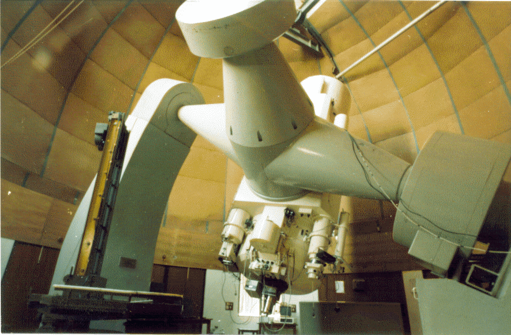
Figure 2.3: The 1.04 m ST at Nainital campus of ARIES. Image credit: 1.04 m ST

2.2.5 1.0 m Nickel Telescope at Lick Observatory

The 1.0 m Nickel telescope is one of the newer telescopes at the Lick observatory. It was built within the Lick observatory workshops at the University of California, Santa Cruz. It has the same optical features as the Cassegrain focus of the 3.0 m Shane telescope mentioned above so that instrument can be shared between these two telescopes. Similar optical features allow instruments designed for the 3 m Shane telescope to be tested at the 1 m Nickel telescope so that the earlier one could be free for research purposes.

The 1 m Nickel telescope has a focal ratio of f/17. Unlike the 3-foci Shane telescope, the f/17 cassegrain focus is the only port available for instrument mounting. This telescope has a modern direct imaging CCD camera of 2K$\times$2K pixels. The CCD has 15 $\mu$m pixels, a plate scale of 0.184^′′ pixel^-1 providing a square FoV of 6.3^′. The available filter wheel with the detector system offers five filter-holding positions. Out of five positions, one is always empty, and the remaining four positions are used to hold the available filters. The $UBVRI$ filters are most commonly employed with this 1 m the available CCD camera. Extensive details on the CCD camera are available at the detector’s homepage.

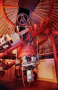
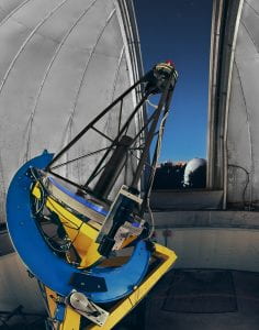
Figure 2.4: Left: The 1 m Nickel telescope at the Lick observatory. Image credit:1 m Nickel; Right: The 0.76 m KAIT at the Lick observatory. Image credit: 0.76 m KAIT.

2.2.6 0.76 m Katzmann Automatic Imaging Telescope (KAIT) at Lick Observatory

The Katzmann Automatic Imaging Telescope is a robotic telescope with a primary mirror spanning a diameter of around 76 cm equipped with a CCD imaging camera. It has a focal ratio of f/8.2 with a plate scale of around 33.2^′′ mm^-1 at its focal plane. It requires minimum human support to look for SNe in the sky throughout each day of the year. This telescope has been optimised to facilitate the early discovery of SNe.

The operation of the 0.76 m KAIT is well organised. It first checks the weather and analyses if the weather conditions are satisfactory for the observations to begin. After that, KAIT opens its dome and starts to observe a preprogrammed list of galaxies to look for new SNe. The newly observed data are compared with previous data from the surveyed area to look for changes. If there are changes that indicate any possible new SN, KAIT automatically emails the astronomers at the University of California, Berkeley. The astronomers at the University of California, Berkeley, follow up by making their own observations to verify the probable SN event. After finishing the observations on the arrival of morning lights, KAIT closes its dome and suspends the activities until the upcoming evening. Extensive details on the KAIT system are provided in Filippenko et al. (2001).

2.2.7 Hubble Space Telescope (HST)

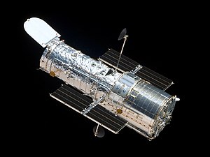
Figure 2.5: The Hubble Space Telescope, figure credit: Hubble Space Telescope.

The Hubble space telescope is the first ever astronomical observatory to be placed in space to orbit around Earth. It is a 2.4 m, f/24 Ritchey-Chretien telescope that can observe near-ultraviolet to optical to near-infrared wavelength range. It utilises two primary camera systems, namely, Advance Camera for Surveys (ACS; installed on HST in 2002) and Wide Field Camera 3 (WFC3; installed on HST in 2009), to obtain photometric observations. Beyond the photometric cameras, the HST is also equipped with several spectrographs. The Space Telescope Imaging Spectrograph (STIS) and the Cosmic Origin Spectrograph (COS) are two complementary instruments mounted on HST that provide detailed spectra of several astronomical sources. Extensive details on the available photometric and spectroscopic instruments systems are provided on the HST instruments homepage.

2.3 Photometric Data Reduction

Photometric data reduction refers to the process of extracting useful information for the sources of interest from photospheric observations stored in raw Flexible Image Transport System (FITS) files. The FITS files store information on the intensity or flux of the astronomical sources. A careful process is required to extract the information by eliminating the spurious signals from the actual signals of interest originating from the desired sources. In this section, we discuss the details of the process of photometric data reduction for the SNe considered in this thesis.

2.3.1 Pre-processing

The raw FITS files from photometric observations are contaminated due to several unwanted signals. The sources of the contaminating signals may be of electric origin or extragalactic. One needs to account for and eliminate these spurious signals from science FITS files to obtain a precise measure of the flux or intensity. The process of removing unwanted signals of electric or extragalactic origin from science frames is known as pre-processing. There are several elements in pre-processing, discussed in detail below:

$\bullet$ Bias correction

The bias is referred to an offset signal present in each pixel of the CCD, even without any incident light. The bias signal act as a source of contamination or noise to the original signal obtained by exposing the CCD for a desired duration and must be subtracted from each frame of interest before any further cleaning.

The process of bias correction starts by obtaining multiple bias frames throughout the course of entire observations in an observing night. A bias frame is acquired with zero-exposure time, keeping the other settings of CCD the same as for obtaining the science images but with the shutter closed. Minor fluctuations in the bias signal level can be eliminated by median combining the multiple bias frames and forming a master-bias frame. To median-combine several bias frames and obtain a master-bias frame, we use the $ZEROCOMBINE$ task from IRAF (Tody, 1986, 1993).

The master-bias frame is then subtracted from each frame obtained through non-zero exposure time. The bias correction process involves the pixel-wise subtraction of the bias value from the corresponding pixel in all other frames with non-zero exposure time. To obtain the bias-corrected frames by subtracting the master-bias from all the non-zero exposure frames, we utilise the $IMARITH$ or $CCDPROC$ task from IRAF. After bias correction, images are free from bias signal and left with astronomical signals containing other sources of noise. Bias correction is an important step as it eliminates the instrumental signature from the data that allows precise measurements of the astronomical signal. It also helps to improve the signal-to-noise ratio (SNR).

$\bullet$ Flat-field correction

Flat correction is another critical step in pre-processing of photometric observational images. When a CCD is exposed to uniform light, all the pixels of the CCD are exposed to nearly the same number of photons. In an ideal case, all the pixels of the CCD should return the same counts, provided they all have similar pixel sensitivity. But, in real scenarios, pixel sensitivity varies. The sources of pixel sensitivity variation are associated with pixel-to-pixel size disparity, deposition of dust grains over the pixels, vignetting effects, etc. Thus, the process of flat correction aims to correct for the uneven illumination and pixel-to-pixel sensitivity variations across the CCD, which can lead to systematic errors in the data.

To correct the pixel-to-pixel sensitivity variation, we must perform the flat-field correction. We obtain several flat frames in different filters by exposing the CCD to a uniform source of light, e.g., the twilight sky during evening and morning. In some cases, dome flat frames are also preferred. The flat frames are obtained in as many filters as the science frames because the responses of the telescope optics system and dust grains are wavelength dependent. Due to this reason, we can not use the flat frames in one filter for other frames with different filters. The flat and science frames are obtained with similar CCD settings. However, exposure durations can be different.

All the flat frames in different filters are first subjected to bias correction. As mentioned earlier, the bias correction is performed through the IRAF tasks $IMARITH$ or $CCDPROC$. Once the bias correction is applied to all the flat frames, we generate the normalised master flat frame for each filter incorporating the $FLATCOMBINE$ task in the IRAF. As a next step, the bias-corrected science frames in each filter are divided by the normalised master flat frame of the corresponding filter. To perform this step, we utilise the $IMARITH$ and $CCDPROC$ tasks in the IRAF. Similar to bias correction, flat correction is exceptionally crucial to perform accurate measurements of astronomical sources.

$\bullet$ Cosmic rays removal

Cosmic rays are highly energetic and charged particles (e.g., positively charged protons, muons, negatively charged electrons, etc.) originating beyond our solar system. These charged particles continuously shower onto our Earth’s atmosphere. The cosmic rays can easily penetrate the dome and telescope system and fall on several CCD pixels producing huge counts in suffering pixels. As the cosmic rays are continuously falling on Earth from several directions all the time, it is very unlikely that any CCD exposure would not suffer from the cosmic ray hits. Cosmic ray removal is an essential step in the pre-processing process for science images, as cosmic rays can create spurious signals affecting astronomical measurements’ accuracy.

The number of cosmic rays hitting a CCD frame depends on the exposure time, although bias frames having zero exposure durations also display some cosmic ray hit features. As mentioned above, cosmic ray hits cause a large count on a single pixel, resulting in a bright spot with different profiles, unlike stellar ones. We utilise the IRAF tasks $COSMICRAYS$ or $CRMEDIAN$ to remove the cosmic rays from all the observed frames. Another option to remove the cosmic rays from photometric frames is by median combining multiple frames as cosmic rays from random directions hit the CCD chip in random positions.

$\bullet$ Image stacking

In several cases, the sources of our interest are not visible in single frames, and we need to stack multiple images of the same filter to detect the source. To detect the source of interest with significant SNR in the science frames, we first need to align and then combine the images of individual filters. To align the science images of a particular band, we utilise the $IMALIGN$ task while the $IMCOMBINE$ task from IRAF is used to stack the aligned images.

$\bullet$ Template subtraction

There are several incidences when an SN occurs close to nuclei or explodes in the bright spiral arm of the host galaxy. In such cases, the SN flux can be significantly contaminated with the flux of the corresponding host galaxy. This situation becomes even more problematic as the SN fades with time. In such situations, magnitude estimations will be erratic if the host galaxy contribution is not eliminated; hence, template subtraction becomes essential to remove the host galaxy contribution. To perform the template subtraction, we need to either obtain the pre-explosion template FITS files of the SN field from the sky surveys or, if the archival template FITS files from sk surveys are unavailable, the template can also be obtained by observing the same supernova field under good observing conditions, once the SN has gone beyond the detection limit of the employed telescope.

With the template image available, we need to do a few checks before subtracting the science images from the template image. First, we need to subtract the median sky background for each science and template image. The sky background counts for the template and science frames are determined at the locations in the images free from any sources. After that, the mean Full-Width-at-Half-Maximum (FWHM) values are constrained for the template and science frames using several bright enough isolated field stars. Between template and science frames, the frame with better FWHM is convolved to match the FWHM of the other so that the two images have similar point spread functions (PSFs). Once the FWHM matching is done, the next task is to match the flux of several sources in the template and science frames near the SN field. Then, a flux scaling factor between the science and template frames is determined. If the flux scaling factor is $>$1, we multiply the scaling factor with the frame with the lower flux or divide it from the frame with the higher flux. As a final step, we subtract the science frame from the template frame, as the science and template frames have achieved similar FWHM and flux values. The final image, resulting from template subtraction, is now ready for photometry.

2.3.2 Photometry

Once pre-processing of the raw data is performed, the science images are ready for photometry to estimate the brightness of the source SN of our interest. Photometry is a fundamental technique in astronomy involving the measurement of the flux of electromagnetic radiation emitted by astronomical sources. It plays an essential role in understanding the behaviours of stars, galaxies, transient events, and other astronomical phenomena. The estimated flux values can be expressed in terms of magnitude units that can be further employed to extract valuable information about the brightness, colour, variability, and other properties of the astronomical sources of interest. Two techniques are there to perform the photometry on a pre-processed science image depending upon the crowding in the considered field:

$\bullet$ Aperture photometry

Aperture photometry is a beneficial and handy technique to estimate the total flux of an astronomical source within a defined aperture. Aperture photometry is preferred to estimate the magnitudes of sources in sparse astronomical fields consisting of uncrowded astronomical sources. In this photometry technique, we select an aperture of a suitable radius around the source of our interest to estimate the associated flux. The selected aperture could be a circular or annular region centred on the source of interest. However, a circular aperture is preferred over an annular one for aperture photometry because the field stars exhibit PSF profiles with functional Moffat, modified Lorentzian, or Gaussian. To find the coordinates of the centre of the selected aperture, we utilise the $CENTERPARS$ task using DAOPHOT available in IRAF. This task fits one of the three functions mentioned above to determine the centre of the selected aperture. The total flux in the defined aperture also consists of sky fluxes; thus, one has to remove the sky fluxes to measure the source flux precisely. To remove the sky background, we use the DAOPHOT $FITSKYPARS$ task in IRAF.

Selecting an appropriate size of the aperture is essential to perform precise photometry. The chosen aperture should be big enough to collect almost all the flux from the source of interest, but at the same time, it should not be very big to introduce additional noises from the sky background and nearby sources. For example, assuming a Gaussian function for the stellar profile, an aperture with a radius of around 3 to 4 times the FWHM of PSF is sufficient to collect more than 99% of the star flux. When estimating the total flux, one can apply an aperture correction to account for the uncertainties associated with determining the appropriate aperture size. One can use the $PHOT$ task of DAOPHOT in IRAF to perform the aperture photometry.

We can summarise the aperture photometry as follow. We identify our source of interest in the field and select an appropriate aperture size. After that, we estimate the sky contributions and subtract that from the total flux in the defined aperture. We can also apply aperture corrections to account for the uncertainties of selecting an appropriate aperture radius. Finally, we perform the aperture photometry with the help of $PHOT$ task of DAOPHOT available with IRAF.

$\bullet$ PSF photometry

Using aperture photometry in a crowded field is unsuitable since the nearby stars can contaminate the photometry of the source of our interest. Additionally, aperture photometry’s linear sky background assumption is invalid in a crowded field. The sources in a crowded field can be so close that their PSFs may overlap, leading to erratic aperture photometry. With these limitations of aperture photometry, PSF photometry is the preferred technique to obtain reliable photometry in a crowded field. The stellar profile extends to several pixels due to atmospheric extinction. The Moffat, modified Lorentzian, or Gaussian functions are used to fit the stellar profiles in the PSF photometry. One of these three functions generates a standard fit to the PSF image by choosing a few bright and isolated field stars. One should be careful that the selected bright star is not saturated. This process of choosing appropriate stars to form the PSF is done using the DAOPHOT task $PSTSELECT$, and the formation of the standard PSF is performed using the DAOPHOT task $PSF$ in IRAF. The FWHM of the stellar profile is utilised to determine the fitting radius, while the fitting parameters are adjusted to match the observed PSF. Additionally, the standard PSF image is scaled to match the PSF in the observed image and subsequently subtracted to isolate the source flux. The PSF magnitude of the object of interest is then estimated using the DAOPHOT $ALLSTAR$ task in the IRAF.

2.3.3 Atmospheric extinction

Atmospheric extinction refers to the phenomena of absorption or scattering of light from astronomical objects by the Earth’s atmosphere. This causes significant attenuation in the observed brightness of those celestial sources. The effect of atmospheric extinction is particularly significant for ground-based observatories. The amount of decrement in the brightness of incoming light passing through Earth’s atmosphere is primarily a function of the wavelength of incoming light, the altitude of the site, and the constituents of the atmosphere. There are two prime mechanisms in Earth’s atmosphere contributing to atmospheric extinction:

$\bullet$ Scattering: Earth’s atmosphere consists of several molecules, aerosols, and other particles capable of scattering the incoming light from celestial objects in all directions. Two types of scattering phenomena occur in Earth’s atmosphere that significantly decrease the intensity of incoming light. The first one is Rayleigh scattering. The coefficient of Rayleigh scattering varies inversely to the fourth power of the incoming light. As a result, blue and violet suffer more scattering than other longer wavelength lights, e.g., red and infrared light. Another type is the aerosol scattering arising from aerosols in Earth’s atmosphere.

$\bullet$ Absorption: A few atmospheric constituents, including ozone, water vapour, and a few other gasses, can selectively absorb specific wavelengths of light. For example, the ozone layer at a height of around 15 to 40 km in the stratosphere significantly absorbs the incoming ultraviolet radiation.

Thus, atmospheric extinction has three main contributors; two from scattering (i.e., Rayleigh and aerosol scattering) and one from absorption. The total extinction coefficient is the sum of these three extinction coefficients. Extensive detail on atmospheric extinction is provided in Hayes & Latham (1975).

In addition to the atmospheric extinction, the local atmospheric conditions of any observatory on several seasons also affect the observations. The relation between the observed magnitude, m($\lambda$,$z$) of any celestial object on the Earth and its magnitude, m₀($\lambda$), outside the Earth’s atmosphere is given by the famous Bouguer’s linear formula as follow:

$$m(\lambda,z)=m_{o}(\lambda)+1.086\times A_{\lambda}\times M(z)$$ (2.1)

Here, $A_{\lambda}$ denotes the wavelength-dependent extinction coefficient, $z$ is the zenith angle, and $M(z)$ represents the airmass at a zenith distance of $z$. Airmass refers to the extent of the Earth’s atmosphere that the light from a celestial object has to traverse when observed from the surface of the Earth along the line of sight. The airmass for a specific astronomical source, assuming a plane-parallel atmosphere, can be obtained using the object’s declination ($\delta$), the observer’s latitude ($\phi$), the zenith angle ($z$), and the hour angle ($h$) at the time of observation. The formula to estimate the airmass is as follows:

$$M(z)=sec(z)=(sin\phi\leavevmode\nobreak\ sin\delta\leavevmode\nobreak\ +\leavevmode\nobreak\ cos\phi\leavevmode\nobreak\ cos\delta\leavevmode\nobreak\ cosh)^{-1}$$ (2.2)

The assumption of a plane-parallel geometry for Earth’s atmosphere is not true. Thus a correction term $\Delta$X is applied in the above Eq. to account for the curvature of the atmosphere. The correction term is given by:

$$\Delta X=0.00186[sec(z)-1]+0.002875[sec(z)-1]^{2}+0.0008083([sec(Z)-1]^{3}$$ (2.3)

With the correction term $\Delta$X, the final airmass equation takes the form as:

$$M(z)=sec(z)-\Delta X$$ (2.4)

Eq. 2.4 indicates that light from any celestial object close to the zenith has to traverse a shorter path than when the same source is near the horizon. As a result, the source at the later position suffers from a higher extinction. In general, the extinction of a celestial source is directly related to the airmass and is also influenced by the wavelength of the incoming light. As mentioned earlier, it is necessary to account for atmospheric extinction and airmass when calculating instrumental magnitudes using aperture or PSF photometry techniques. This correction is applied to transform the measured magnitudes to what they would be if the observations were conducted outside the atmosphere. The formula for this correction is as follows:

$$m_{\lambda}^{0}=m_{\lambda}-A_{\lambda}\times M(z)$$ (2.5)

In this Eq., $m_{\lambda}^{0}$ represents the instrumental magnitude at zero airmass (corresponding to the value if the observations were conducted outside the Earth’s atmosphere), $m_{\lambda}$ represents the instrumental magnitude at a specific airmass.

2.3.4 Photometric Calibration

The instrumental magnitude of a source obtained through different photometric systems would be different. A photometric system comprises a telescope equipped with a filter and detector system at any observatory. We need to transform or calibrate the instrumental magnitudes to some standard system to use those magnitudes from different photometric systems together. The process of converting photometric system-dependent instrumental magnitudes to an independent standard system is known as photometric calibration. Once calibrated to a standard system, the magnitudes from several photometric systems can be used together for further analysis.

Along with the science frames, several photometric standard stars with a range of colours and brightnesses should also be observed under good observing conditions. The transformation from instrumental to calibrated magnitudes can be done through colour-colour or colour-magnitude transformation equations. In the present thesis, we have mainly employed the transformation equations from Stahl et al. (2019) and Kumar et al. (2022b).

2.4 Spectroscopic Data Reduction

Spectroscopy in astronomy refers to the study of the variation of the flux of a celestial object in small wavelength bins. When light passes through a medium (e.g., gas or a cloud of dust), it interacts with the atoms, ions, and molecules present in the medium. These interactions cause certain wavelengths of light to be absorbed or emitted, which are reflected as absorption or emission feature in the spectrum. This is the basic principle behind spectroscopy. To observe and record the spectra of a source, spectrographs are attached with the telescopes. Spectrographs are instruments with the ability to disperse light into its component wavelengths. Spectroscopy is an excellent method for exploring the chemical composition of celestial sources and extracting crucial information such as surface gravity, radial velocities, redshift, metallicity, and many more. Under the context of the present thesis, we have conducted a comprehensive analysis utilising slit-based low-resolution spectroscopic data of several CCSNe. These observations were made possible through the utilisation of many telescopes and detectors, enabling a detailed investigation of the physical and chemical properties of these catastrophic explosions.

The spectrograph receives light from the celestial object, which is then dispersed perpendicular to the slit axis, referred to as the “dispersion axis”. The slit serves the purpose of blocking unwanted light and selectively collecting light from the source of our interest. In a specific observation, the optimal width of the slit is selected to match the seeing-limited FWHM. The dispersion axis carries valuable information about the distribution of flux along the spatial axis of the CCD.

To ensure precise wavelength and flux calibrations, the spectra from arc lamps such as Fe-Ar, Fe-Ne, and Neon, as well as standard star spectra, are also obtained. Additionally, bias and flat frames are also acquired to facilitate preprocessing of the raw CCD data. The subsequent subsections will outline the primary steps followed during the process of spectroscopic data reduction.

2.4.1 Pre-processing

As mentioned previously, while discussing the pre-processing of photometric data, it is also mandatory to preprocess the raw spectroscopic data to eliminate the CCD artefacts and cosmic ray hits. Thus, the spectroscopic data also deal with bias, flat, and cosmic ray corrections. Techniques similar to photometric data preprocessing are employed for bias and cosmic ray hit corrections. However, instead of using uniformly illuminated twilight sky flat frames, halogen lamp spectra are obtained for applying the flat correction.

To create the master flat frame, multiple bias-corrected halogen lamp frames are median combined using the $FLATCOMBINE$ task in IRAF. The next step involves generating a normalised flat frame. This is achieved by fitting a high-order spline function to the halogen spectrum extracted from the master flat frame, utilising the $RESPONSE$ task in IRAF. The fitted function is then divided to the master flat frame to produce the normalised master flat frame.

Applying the flat correction involves dividing the normalised master flat frame from the bias-corrected arc-lamp frames, standard star frames, and science frames. This is accomplished using the $IMARITH$ task in IRAF. Additionally, to account for the non-linear behaviour typically observed at the edges of the CCD, any necessary trimming of the 2-dimensional spectrum edges can be performed using the $IMCOPY$ task in IRAF.

2.4.2 Spectrum extraction

In this section, we discuss the process of extracting a 1-dimensional spectrum from a pre-processed 2-dimensional spectroscopic image. The first step for extracting the spectrum involves the identification of a dispersion line. Generally, the dispersion line is expected to be located in the middle of the spatial axis. However, to determine its precise location, a cut is made along the spatial axis, and the peak coordinates of the Gaussian profile are recorded. Once we identify the centre of the dispersion line, the next step involves extracting the aperture and subtracting the background.

The aperture, characterised by its base-to-base width and peak, can be easily traced as the cross-section of the dispersion line or the stellar profile has a Gaussian-like shape. Background windows are selected on either side of the Gaussian peak. A low-order “Chebyshev function” is employed to estimate the background profile, which is then subtracted from the aperture along that column.

It is important to consider that the dispersion line is not exactly perpendicular to the spatial axis of the CCD due to geometric distortions caused by telescope optics, grating alignment, and the gradient of atmospheric refraction with respect to the wavelength. Consequently, we generate the 1-dimensional spectrum along the dispersion axis by extracting the peak counts along the dispersion axis and subsequently summing them across the spatial axis.

All the above-mentioned tasks to extract the 1-dimensional spectrum can be performed using the $APALL$ task in IRAF. Extracting the standard star spectra observed on the same night also follows a similar procedure. However, the extraction of arc lamp spectra for the wavelength calibration of the object and standard star spectra is performed with the same trace and centring position. To obtain this, the $APALL$ task is used again, with the object or standard star spectrum as the reference. The extracted spectrum of the source of interest consists of pixel numbers versus count values, which need to be converted into wavelength and flux. We perform the wavelength and flux calibration tasks to achieve these conversions.

2.4.3 Wavelength and Flux calibration

$\bullet$ Wavelength calibration

This task aims to transform the pixel numbers on the x-axis of the extracted spectrum into wavelength units. The arc-lamp spectra have several characteristic emission features with precisely known corresponding wavelengths. Utilising the $IDENTIFY$ task in IRAF, these emission features can be easily identified. The line identification output data are fitted using low-order polynomials to prepare the pixel-to-wavelength mapping solution. Further, we use the fitted polynomial onto other 1-dimensional spectra of the source and standard stars utilising the $DISPCOR$ task in IRAF. As a result, we obtain the wavelength-calibrated spectra of the source of interest and standard stars.

$\bullet$ Flux calibration

The flux calibration task aims to transform the y-axis instrumental counts of the wavelength-calibrated spectrum to flux units (i.e., in units of erg s^-1 cm^-2 Å^-1). To establish the relationship between CCD counts and flux at different wavelengths, we utilise the standard-star spectra and employ splines to fit the continua. This fitting process gives sensitivity functions that provide a mapping from CCD counts to flux for each specific wavelength. Finally, these sensitivity functions are utilised to calibrate and adjust the flux values in each individual spectrum of the source of our interest. The detailed processes of wavelength and flux calibration are achieved utilising IRAF routines and custom Python and IDL-based scripts. These processes are explicitly described in Silverman et al. (2012).

2.5 Supernova Progenitor Modelling Using the Modules for Experiments in Stellar Astrophysics (MESA)

MESA, the acronym for the Modules for Experiments in Stellar astrophysics (Paxton et al., 2011, 2013, 2015, 2018, 2019; Jermyn et al., 2023) represents a collection of powerful, open-source libraries designed to serve to a diverse range of computational needs within the realm of stellar astrophysics. These libraries are well known for their reliability, efficiency, and ability to operate seamlessly in multi-threaded environments. MESA can tackle a diverse range of astrophysical situations. It is capable of performing the stellar evolution of very low mass stars to very old ages, can evolve massive stars from pre-main sequence up to the core-collapse stage, evolve very massive stars to the PISN or PPISN stages depending upon their masses, and also capable of simulating the evolution of accretion onto an NS. Thus, MESA can mimic various astrophysical events ongoing in our Universe. However, within the context of the research work in the presented thesis, we have utilised MESA to evolve massive stars (M_ZAMS $>$ 8 M_⊙) from pre-main sequence up to the onset of core collapse. These models at the stage of the beginning of core collapse serve the purpose of inputting pre-SN models to other simulation tools that simulate their synthetic, hydrodynamic explosions.

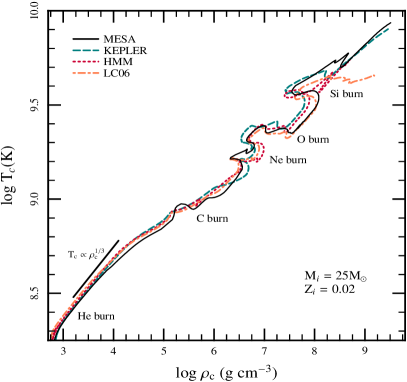
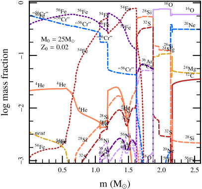
Figure 2.6: Left: The variation of the core temperature against core density as the 25 M_⊙ model with Z $=$ 0.02 evolves through various stages of burning in its core is shown. The results of other available evolutionary codes are also shown for comparison. Right: The mass fractions of several species at the stage of the onset of core collapse are shown. The figures are adapted from Paxton et al. (2011).

The capability of MESA to simulate the stellar evolution of a massive star starting from pre-main sequence up to the onset of core collapse is well documented in Paxton et al. (2011). The authors of Paxton et al. (2011) have evolved a 25 M_⊙ ZAMS mass star up to the onset core collapse stage. They have studied the evolution of the model on the HR diagram. The authors have also investigated the variation of the core-temperature versus core-density curve (as shown in the left-hand panel of Figure 2.6) throughout the entire evolution of the model. They have also studied models’ mass fractions (as shown in the right-hand panel of Figure 1.2) at the onset of the core collapse stage. With these capabilities, MESA caters to excellent opportunities to investigate the entire evolution of massive stars.

2.6 Tools to Simulate the Synthetic Explosions of pre-SN Models

Once the models have arrived at the stage of the onset of core collapse, we can utilise the output of MESA in appropriate form as input to other SN explosion codes capable of simulating the synthetic explosions of the MESA pre-SN models. There are several codes available to simulate synthetic explosions from pre-SN models. However, we have utilised two codes for the research work performed in the present thesis mentioned below:

2.6.1 SuperNova Explosion Code (SNEC)

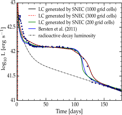
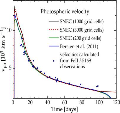
Figure 2.7: Left: The comparison of SNEC generated bolometric light curves with actual observations of SN 1999em are shown. The effect of increasing grid cells is also explored. Right: The comparison of corresponding SNEC generated velocity evolutions is compared with actual Fe II line velocities of SN 1999em. The results of Bersten et al. (2011) are also shown for comparison purposes. Figure credit: Morozova et al. (2015).

SNEC, the acronym for SuperNova Explosion Code Morozova et al. (2015) is a publicly available, 1-dimensional Lagrangian hydrodynamic code. SNEC solves the radiation energy transport equation within the flux-limited diffusion approximation to simulate the synthetic explosion of pre-SN models. To synthetically explode the pre-SN model, SNEC requires structure and chemical composition information. Thus, once a certain mass ZAMS model has reached the onset of the core collapse stage using MESA, the pieces of information regarding the structure and chemical composition of the pre-SN model are mapped in the appropriate form, and those pieces of information serve as input to SNEC, that explodes the pre-SN model.

The setups for the explosion in SNEC are controlled by a file named parameters. The type of explosion, explosion energy, ⁵⁶Ni mass, ⁵⁶Ni distribution within the model, the mass of the excised core, number of grid cells, duration upto which the light curves are generated etc., are controlled by the user in the parameters file. For the explicit details on the working of SNEC and underlying explosion parameters, one should consider Morozova et al. (2015). After finishing the calculation, the code generates the bolometric light curve, multi-band light curves, and the photospheric velocity evolution of the SN, along with a few more physical and chemical characteristics. The model-generated light curves and velocity evolution are compared with actual observations as shown in the left- and right-hand panels of Figure 2.7.

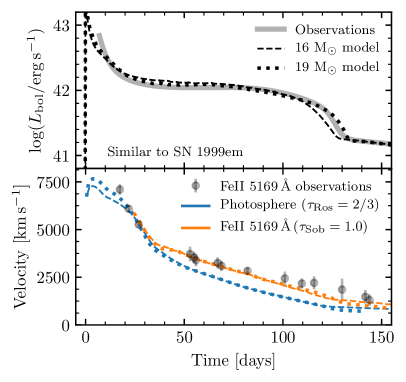
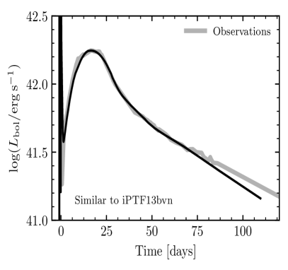
Figure 2.8: Left: The comparison of STELLA generated bolometric light curves with actual observations (top panel) of SN 1999em are shown. The comparison of corresponding velocity evolution is also shown (bottom panel). Right: The capacity of STELLA to model a few stripped envelope is displayed. This figure compares the STELLA produced bolometric light curve with a Type Ib SN iPTF13bvn observations. Figure credit: Paxton et al. (2018).

2.6.2 STELLA

STELLA (Blinnikov et al., 1998, 2000, 2006) is another 1-dimensional multi-group radiation hydrodynamics code. A simplified version of STELLA is available publicly in MESA. In contrast to SNEC, it tackles the radiative transfer equations through the intensity momentum approximation in each frequency bin. Within MESA, the utilisation of STELLA commonly involves employing a maximum of 40 frequency groups. This selection of 40 frequency bins equips STELLA with the ability to generate SEDs of exploding models; however, with 40 frequency bins, STELLA fails to produce complete spectra. Extensive details on massive star explosions and utilisation of STELLA to generate bolometric luminosity light curves, multi-band light curves, and velocity evolutions are well documented in Paxton et al. (2018). The utilisation of STELLA to model the observations of H-rich and H-deficient CCSNe is shown in the left- and right-hand panels of Figure 2.8.

Chapter 3 Constraints on the progenitor masses of two Type Ib Supernovae, SN 2015ap and SN 2016bau

3.1 Current Understanding in the Research Area

As detailed in earlier Chapters 1 and 2, CCSNe are among the most powerful astronomical explosions, occurring during the final stellar evolutionary stages of massive stars having initial mass $\geqslant$8 M_⊙ (Gilmore, 2004; Woosley & Janka, 2005; Groh, 2017)). Knowledge of the possible progenitors of CCSNe is one of the most fundamental tasks in understanding these catastrophic explosions. Therefore, in this Chapter, we aim to explore the origins of the underlying progenitors of two Type Ib CCSNe by analysing their photometric and spectroscopic data along with simulations involving hydrodynamic modelling of their explosions.

Due to the limited understanding of the potential progenitors of H-stripped CCSNe, people have started paying special attention to this research area. For SNe Ib/c, broadly, two scenarios are proposed for their progenitor system. The first involves relatively low-mass progenitors ($>$ 11 M_⊙) in binary systems (Podsiadlowski et al., 1992; Nomoto et al., 1995; Smartt, 2009), where the primary star lost its H-envelope through the transfer of mass to a companion star. The second considers massive WR stars ($>$ 20–25 M_⊙) that lose mass via stellar winds (e.g., Gaskell et al., 1986; Eldridge et al., 2011; Groh et al., 2013). For a Type Ib SN iPTF13bvn, the authors of Cao et al. (2013) reported the detection of a possible progenitor in pre-explosion images within a 2$\sigma$ error radius, consistent with a massive WR progenitor star. Stellar evolutionary models also support the massive WR progenitor scenario. Based on observational evidence from early- and nebular-phase spectroscopy of SNe Ib, both massive WR stars and interacting binary progenitors are proposed. The hydrodynamic modelling of the possible progenitors (identified either via direct imaging as in the case of iptf13bvn (Cao et al., 2013) or indirect methods which include nebular-phase spectral modelling Jerkstrand et al. 2015; Uomoto 1986) and simulating their synthetic explosions can be vital to understanding their nature, physical conditions, circumstellar environment, and chemical compositions. Unfortunately, only a handful of such studies have been performed in the cases of stripped-envelope SNe, including the Type Ib SN iptf13bvn (Cao et al., 2013; Bersten et al., 2014; Paxton et al., 2018), the famous Type IIb SN 2016gkg (Bersten et al., 2018), and the Type IIb SN 2011dh (Bersten et al., 2012). Our work takes such studies one step further as we perform the stellar evolution of the possible progenitors of two new SNe Ib and simulate their synthetic explosions.

Another aspect of CCSNe is understanding the underlying powering mechanisms behind their light curves. The main powering mechanism in normal SNe Ib/c is radioactive decay of ⁵⁶Ni and ⁵⁶Co, leading to the deposition of energetic gamma rays that thermalise in the homologously expanding ejecta (e.g., Arnett, 1980, 1982, 1996; Nadyozhin, 1994; Chatzopoulos et al., 2013; Nicholl et al., 2017). Some SNe Ib (e.g., SN 2005bf, Maeda et al. 2007) have also shown evidence for the light curves being powered by the spin-down of a young magnetar (e.g., Ostriker & Gunn, 1971; Arnett & Fu, 1989; Maeda et al., 2007; Kasen & Bildsten, 2010; Woosley, 2010; Chatzopoulos et al., 2013; Nicholl et al., 2017). In the post-photospheric phase, when the SN ejecta become optically thin, the light curves of CCSNe are powered by energy deposition from the radioactive decay of ⁵⁶Ni to ⁵⁶Co and finally to ⁵⁶Fe. In many cases, however, the SN progenitor is embedded within dense circumstellar matter (CSM), so when the SN explosion occurs, the SN ejecta may violently interact with the CSM, resulting in the formation of forward and reverse shocks that deposit their kinetic energy into the material which is radiatively released and thus powers the light curve (e.g., Chevalier, 1982; Chevalier & Fransson, 1994; Moriya et al., 2011; Ginzburg & Balberg, 2012; Chatzopoulos et al., 2013; Nicholl et al., 2017).

In this Chapter, we explore the photometric and spectroscopic behaviour of SN 2015ap and SN 2016bau, primarily using the data obtained using the KAIT, Nickel, and Shane telescopes at Lick Observatory. Based on the analysis, we model and attempt to place constraints on the properties of the progenitors of these two SNe. In Sec. 3.2, details about various telescopes and reduction procedures are presented. Sec. 3.3 provides methods to correct for the Milky Way and the host-galaxy extinction. Photometric properties of the two SNe, such as their bolometric light curve, temperature, radius, and velocity evolution, are also discussed. Sec. 3.4 includes the analysis describing the spectral evolution of SN 2015ap and SN 2016bau, as well as comparisons with other similar and well-studied SNe; we also model the spectra of these SNe using SYN++. In Sec. 3.5, we have modelled the multi-band light curves of SN 2015ap and SN 2016bau utilising MOSFiT. Further, quasi-bolometric light-curve modelling is performed in Sec. 3.6; light curves corresponding to various powering mechanisms of SNe are fitted to the observed quasi-bolometric light curves. The assumptions and methods for modelling the possible progenitors of the two SNe and their evolution until the onset of core-collapse using MESA are presented in Sec. 3.7. We discuss the assumptions and methods for producing the synthetic explosions using SNEC and STELLA in Sec. 3.8; here, the comparisons between the parameters obtained through synthetic explosions and observed ones are presented. In Sec. 3.9, we discuss our analysis’s major results and findings. Finally, in Sec. 3.10, we summarise our work by briefly discussing the major outcomes and providing concluding remarks.

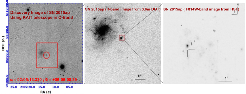
Figure 3.1: Left panel: The discovery image of SN 2015ap using the KAIT telescope in $C$-filter. The SN is marked inside the red circle. Middle panel: A zoomed version of an $R$-band image with $2^{\prime}\times 2^{\prime}$ FoV obtained on 6 Oct. 2020 using the 4K$\times$4K CCD imager mounted on the 3.6 m DOT. Right panel: A further zoomed, about $6^{\prime\prime}\times 6^{\prime\prime}$ FoV of the location of SN 2015ap taken on 12 Aug. 2020 using the HST in the F814W filter. The SN seems to be fainter than the detection limit of the HST at this time. A log of HST observations is included in the Appendix.

3.2 Data acquisition and reduction

SN 2015ap was discovered by KAIT as part of the Lick Observatory Supernova Search (LOSS; Filippenko et al., 2001), in an 18 s unfiltered image (close to the $R$ band; see Li et al. 2003) taken at 11:16:31 on 2015 Sep. 08 (Ross et al., 2015), at 17.41$\pm$0.06 mag. The object was also marginally detected one day earlier on Sep. 07.47 with 18.07$\pm$0.22 mag. We measure its J2000.0 coordinates to be $\alpha=02^{\rm h}05^{\rm m}13.^{\rm s}32$, $\delta=+06^{\circ}06^{{}^{\prime}}08.^{{}^{\prime\prime}}4$, with an uncertainty of $0.^{{}^{\prime\prime}}5$ in each coordinate. SN 2015ap is $28.^{{}^{\prime\prime}}3$ west and $16.^{{}^{\prime\prime}}2$ south of the nucleus of its host galaxy IC 1776, which has a redshift of $z$ = 0.011375$\pm$0.000017 (Chengalur et al., 1993) and a barred-spiral (SB(s)d) morphology as mentioned in de Vaucouleurs et al. 1991. SN 2016bau was discovered by Ron Arbour in an unfiltered image taken at 23:22:33 on 2016 Mar. 13 (Arbour, 2016), at 17.8 mag. Its J2000.0 coordinates are given as $\alpha=11^{\rm h}20^{\rm m}59.^{\rm s}02$, $\delta=+53^{\circ}10^{{}^{\prime}}25^{{}^{\prime\prime}}6$. SN 2016bau is $35.^{{}^{\prime\prime}}3$ west and $15.^{{}^{\prime\prime}}2$ north of the nucleus of its host galaxy NGC 3631, which has $z$ = 0.00384$\pm$0.00014 (Falco et al., 1999) and a morphology of SAc C (Ann et al., 2015). Both of these SNe were classified as SN Ib based on well-developed features of He I, Fe II (blended), and Ca II, a few days after maximum brightness.

Figure 3.1 shows finder charts of SN 2015ap obtained with different telescopes. In the HST image, for the location of SN 2015ap and the cluster from which it came, astrometry was done between the ground-based image (picked up from the ESO archive) and the HST image. A coordinate transformation was performed between the two images, which allowed the position of the SN to be found. Then, photometry was done using DOLPHOT (Dolphin, 2000, 2016), a photometry pipeline developed for HST data. While the SN was not found in this finder chart, we outlined only the star cluster close to the reported position of SN 2015ap.

The $B$, $V$, $R$, and $I$ follow-up images of SN 2015ap and SN 2016bau were obtained with both the 0.76 m KAIT and the 1 m Nickel telescope at the Lick Observatory. We reduced all the images using a custom pipeline detailed by Stahl et al. (2019). Here, we briefly summarise the process of photometry. Image subtraction techniques were employed to eliminate the background light from the host galaxy, utilising supplementary images acquired subsequent to the SN’s decline below our detection threshold. Point-spread-function (PSF) photometry was executed through the utilization of DAOPHOT (Stetson, 1987) from the IDL Astronomy User's Library. Three nearby stars were chosen from the Pan-STARRS1 catalogue for calibration. The magnitudes of these objects were initially converted to Landolt (1992) magnitudes using the empirical prescription presented by Tonry et al. (2012, Eq. 6) and thereafter converted to the KAIT/Nickel natural system. We measured all the apparent magnitudes in the KAIT4/Nickel2 natural system. The ultimate outcomes were then transformed to the standard system using local reference sources and accounting for colour terms for KAIT4 and Nickel2, as documented by Stahl et al. (2019). In addition, the $U$-band photometry was obtained from the Swift Optical/Ultraviolet Supernova Archive (SOUSA; https://archive.stsci.edu/prepds/sousa/; Brown et al. 2014).

There are a total of 17 spectra of SN 2015ap; 15 of them were taken with the Kast spectrograph (Miller & Stone, 1993) on the 3 m Shane telescope at Lick Observatory and the other 2 were taken with LRIS (Oke et al., 1995) on the Keck-I 10 m telescope. Except for the earliest spectrum taken on 10.531 Sep. 2015 (UT dates are used throughout this Chapter) using the Lick Shane/Kast system, 16 spectra in this Chapter were published by Shivvers et al. (2019); refer to that paper for details of the observations. Also, there are 8 spectra of SN 2016bau, all obtained with the Lick Shane/Kast system. We used the 600/4310 grism on the blue side, the 300/7500 grating on the red side, the d5500 dichroic, and a long slit $2^{\prime\prime}$ wide. For LRIS we used the 600/4000 grism on the blue side, the 400/8500 grating on the red side, and a $1^{\prime\prime}$ slit. The spectra were binned to 2 Å pixel^-1.

3.3 Photometric Properties

In this section, we discuss various photometric properties of SN 2015ap and SN 2016bau, including their colour evolution, extinction, quasi-bolometric light curves, and various blackbody parameters.

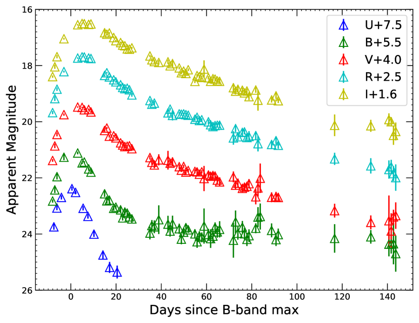
Figure 3.2: $UBVRI$ light curves of SN 2015ap, where $BVRI$ data were obtained with KAIT while the $U$-band data were taken from the UVOT mounted on Swift (https://swift.gsfc.nasa.gov).

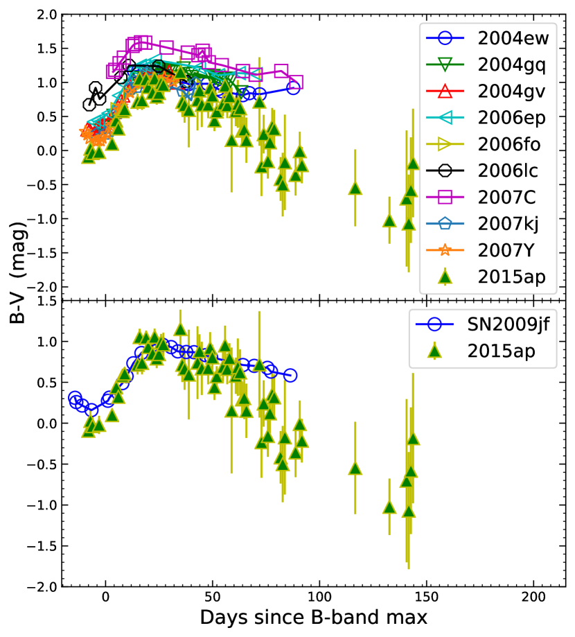
Figure 3.3: The top panel shows a comparison of the $(B-V)$ colour of SN 2015ap (corrected for Milky Way extinction) with that of other Type Ib SNe. The data for SNe other than SN 2015ap are taken from Stritzinger et al. (2018). The bottom panel shows the $(B-V)$ colour curves of SN 2015ap and SN 2009jf (both corrected for Milky Way extinction).

3.3.1 Photometric behaviour of SN 2015ap

Most of the analysis in this Chapter has been performed with respect to $B$-band maximum brightness. To find its date, we fit a sixth-order polynomial to the $B$ data sampling the photospheric phase. The resulting date of $B$-band maximum is MJD 57282.47$\pm$2.56. To determine the explosion epoch ($t_{\rm exp}$) of SN 2015ap, we use $R$-band data. The $R$ magnitudes are converted into fluxes, and a sixth-order polynomial is fitted. We extrapolate the polynomial, and the epoch corresponding to zero flux is taken as the explosion epoch, MJD 57272.72$\pm$1.49, which is in good agreement with Prentice et al. (2019).

Figure 3.2 shows the $UBVRI$ light curves of SN 2015ap. The rising rate for the $U$-band light curve is faster than that of other bands, and similarly, the $U$ decline rate is faster, making the $U$ light curve much narrower compared to other bands. As we go to longer wavelengths, we see that the light curves become broader, with the $I$-band light curve being the broadest.

$\bullet$ Colour evolution and extinction correction

Distances are taken from the NASA Extragalctic Database (NED), and a cosmological model with H₀ = 73.8 km s^-1 Mpc^-1, $\Omega_{m}$ = 0.3, and $\Omega_{\Lambda}$ = 0.7 is assumed throughout. For SN 2015ap, we corrected for Milky Way (MW) extinction using NED following Schlafly & Finkbeiner (2011). In the direction of SN 2015ap, the Galactic extinctions for the $U$, $B$, $V$, $R$, and $I$ bands are 0.185, 0.154, 0.117, 0.092, and 0.064 mag, respectively.

The top panel of Figure 3.3 shows a comparison of the $(B-V)$ colour of SN 2015ap with that of other Type Ib SNe (all corrected for MW extinction). SN 2015ap seems to be the least reddened and lies below nearly all of the other SNe Ib.

Following Prentice et al. (2019), the host-galaxy contamination is negligible and hence ignored. To further support this assumption, the $(B-V)$ colour curve of SN 2009jf (Sahu et al., 2011) is shown in the bottom panel of Figure 3.3, corrected for an MW colour excess of $E(B-V)_{\rm MW}=$ 0.112 mag (host extinction is negligible). In order to match the ($B-V$) colour curve of SN 2009jf, we need not apply any shift to the MW-corrected SN 2015ap $(B-V)$ colour curve.

Figure 3.4 illustrates the position of SN 2015ap in the Miller diagram (Richardson et al., 2014). The distance modulus ($\mu$) of SN 2015ap is 33.269 mag; thus, SN 2015ap appears to be a normal SN Ib. For SN 2016bau, we calculate $\mu=$ 32.65 mag; based on its position in Figure 3.4, it seems to be a moderately luminous, normal SN Ib.

$\bullet$ Quasi-bolometric and bolometric light curves

To obtain the quasi-bolometric light curves, we used the superbol code (Nicholl, 2018). We first provided the extinction-corrected $U$, $B$, $V$, $R$, and $I$ data to superbol. Thereafter, it mapped the light curve in each filter to a common set of times through the processes of interpolation and extrapolation. It then fits blackbody curve to the spectral energy distribution (SED) at each epoch, up to the observed wavelength, to give the quasi-bolometric light curve by performing trapezoidal integration. The peak quasi-bolometric luminosity obtained through integrating the flux over a wavelength range of 4000–10,000 Å  is $10^{(42.548\pm 0.019)}$ erg s^-1, in agreement with Prentice et al. (2019).

Figure 3.5 shows a comparison of the quasi-bolometric light curve of SN 2015ap with that of other H-stripped CCSNe. The code superbol also provides the bolometric light curve, including the additional blackbody corrections to the observed quasi-bolometric light curve, by fitting a single blackbody to observed fluxes at a particular epoch and integrating the fluxes trapezoidally for a wavelength range of 100–25,000 Å. The top panel of Figure 3.6 provides the resulting quasi-bolometric and bolometric light curves of SN 2015ap.

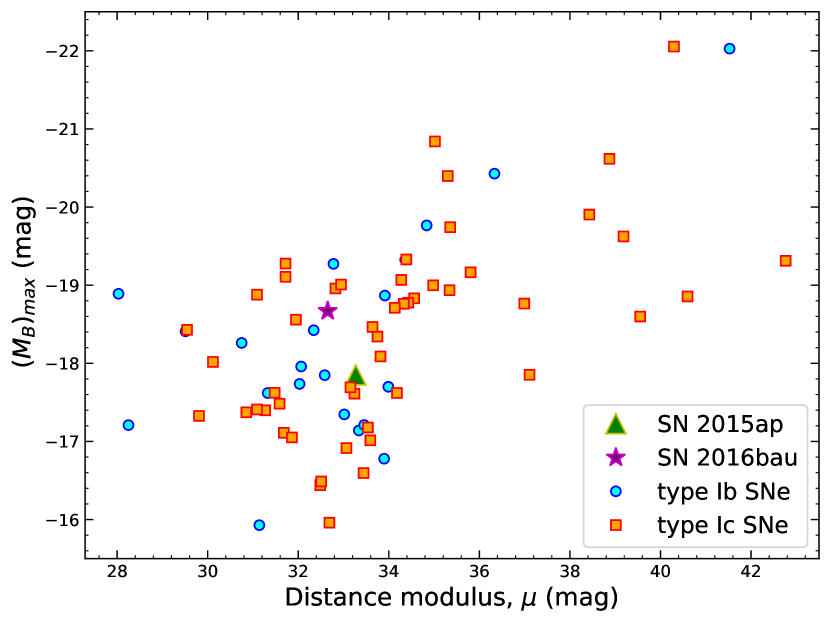
Figure 3.4: The position of SN 2015ap and SN 2016bau in the Miller diagram.

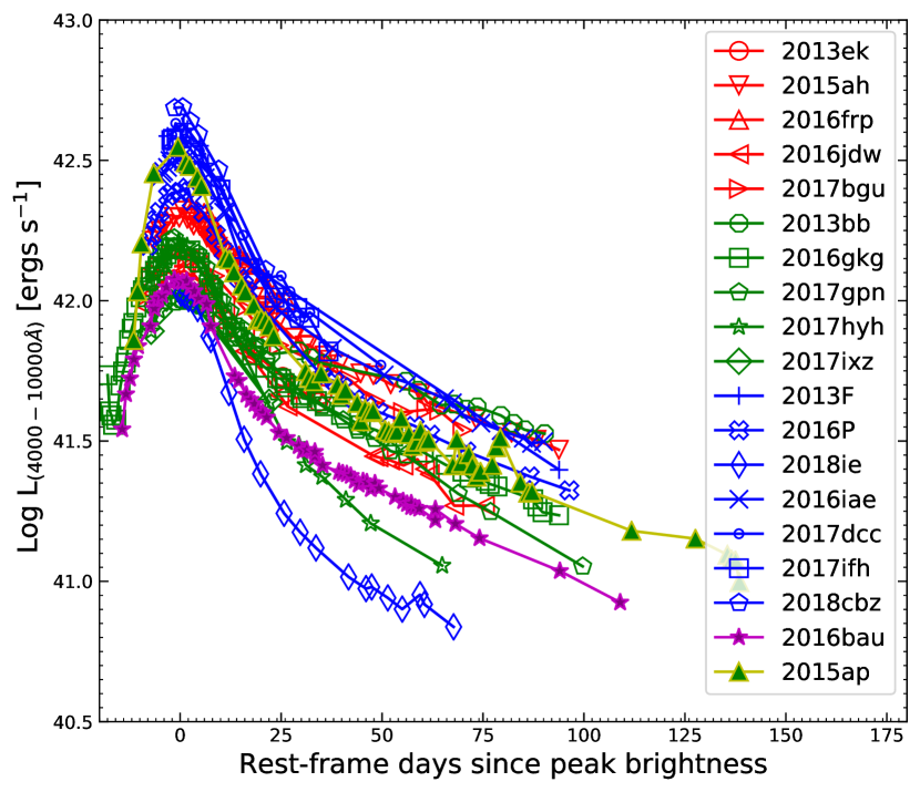
Figure 3.5: Comparison of quasi-bolometric light curves of SN 2015ap and SN 2016bau, obtained by fitting a blackbody to the SED and integrating the fluxes over the wavelength range of 4000–10,000 Å  with other stripped-envelope CCSNe. Symbols are colour coded: red, green, and blue correspond to Type Ib, IIb, and Ic SNe, respectively.

$\bullet$ Temperature, radius, and velocity evolution

From superbol, the photospheric temperature ($T_{\rm BB}$) and radius ($R_{\rm BB}$) evolution of SN 2015ap are also obtained. During the initial phases, the photospheric temperature is high, reaching about 11,400 K at $-6.18$ d. Further, as the SN ejecta expand, cooling occurs and the temperature tends to fall, dropping to 4490 K on +21.66 d, then remaining nearly constant (Fig. 3.6, second panel from top). A conventional evolution in radius is also seen. Initially, at an epoch of -8 d, the photospheric radius is 4.14$\times$ 10¹⁴ cm. Thereafter, the SN expands and its radius increases, reaching a maximum radius of 3.27$\times$10¹⁵ cm, beyond which the photosphere seems to recede into the SN ejecta (Fig. 3.6, third panel from top). From the prior knowledge of the explosion epoch and radii at various epochs, we can estimate the photospheric velocity evolution of this SN, using $v_{\rm ph}=R_{\rm BB}/t$, where $t$ is the time since the explosion. The bottom panel of Figure 3.6 shows the velocity evolution of SN 2015ap.

From the known value of $t_{\rm exp}$, a rise time ($t_{\rm rise}$) of 14.8$\pm$2.2 d is obtained. The photospheric velocity near maximum light is 9000 km s^-1 (Prentice et al., 2019). With the known values of $t_{\rm rise}$, the photospheric velocity near maximum light, and a constant opacity ($\kappa$) of 0.07 cm² g^-1, we also obtain the ejecta mass ($M_{\rm ej}$) and kinetic energy ($E_{\rm ke}$) from the Arnett (1982) model by following Equations (1) and (3) of Wheeler et al. (2015): 2.2$\pm$0.6 M_⊙ and (1.05$\pm$0.31)$\times$10⁵¹ erg, respectively. Our derived ejecta mass is slightly higher than that of Prentice et al. (2019), but less than Gangopadhyay et al. (2020). Corresponding to a peak luminosity of (3.53$\pm$0.16)$\times$10⁴² erg s^-1, the amount of ⁵⁶Ni synthesised is 0.14$\pm$0.02 M_⊙, calculated following Prentice et al. (2016). Precise measurement of the amount of ⁵⁶Ni generated in a CCSN is vital in deducing various progenitor scenarios and explosion processes associated with different CCSNe, as it heavily relies on both the explosion characteristics and the core structure of the underlying progenitor. Consequently, the measurement of nickel production plays an essential role in understanding the progenitors of CCSNe and their explosion mechanisms (Suwa et al., 2019).

Figure 3.6: The top panel shows the bolometric and quasi-bolometric light curves of SN 2015ap. Second panel: the temperature evolution of SN 2015ap. Third and fourth panels: the radius and velocity evolutions (respectively) obtained using blackbody fits.

3.3.2 Photometric properties of SN 2016bau

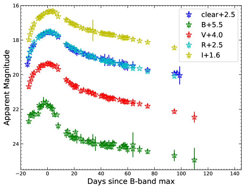
Figure 3.7: $BVRI$ and Clear filter light curves of SN 2016bau.

Following a method similar to that for SN 2015ap, the $B$-band maximum and the explosion epochs of SN 2016bau were determined to be MJD 57477.37$\pm$1.99 and MJD 57462.54$\pm$0.97, respectively. Figure 3.7 shows the $BVRI$ and Clear ($C$) filter light curves of SN 2016bau. Light curves in the shorter-wavelength bands are narrower compared to those in the longer-wavelength bands, following a trend similar to that of SN 2015ap. Also, the $C$ filter almost exactly replicates the $R$-band light curve, as expected (Li et al., 2003).

$\bullet$ Colour evolution and extinction correction

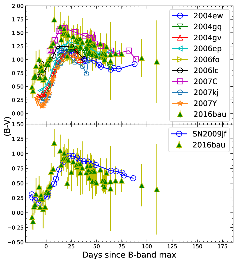
Figure 3.8: The top panel shows a comparison of the $(B-V)$ colour of SN 2016bau with that of other SNe Ib (all corrected for MW extinction). The data for the other SNe are taken from Stritzinger et al. (2018). The bottom panel shows the $(B-V)$ colour curves of SN 2016bau and SN 2009jf, both corrected for MW extinction. To match the SN 2009jf colour curve, a shift of 0.566 mag is required for the SN 2016bau colour curve.

Similar to SN 2015ap, we corrected for MW extinction using NED following Schlafly & Finkbeiner (2011). In the direction of SN 2016bau, the Galactic extinction for the $B$, $V$, $R$, and $I$ bands is 0.060, 0.045, 0.036, and 0.025 mag, respectively. The top panel of Figure 3.8 shows a comparison of the $(B-V)$ colour of SN 2016bau with that of other SNe Ib. SN 2016bau seems to be heavily reddened and lies above nearly all of the other SNe Ib. To correct the host-galaxy extinction, we made use of the colour curve of SN 2009jf. We calculated the differences in the colours of the two SNe and took their weighted mean. In this calculation, we made use of data only in the range 0 to +20 d for the reasons mentioned by Stritzinger et al. (2018). The resulting host-galaxy extinction is $E(B-V)_{\rm host}=$ 0.566$\pm$0.046 mag. Thus, in order to match the SN 2009jf $(B-V)$ colour curve, we need to shift the MW-corrected $(B-V)$ colour curve of SN 2016bau downward by 0.566 mag, as shown in the bottom panel of Figure 3.8.

$\bullet$ Quasi-bolometric and bolometric light curves

To obtain the quasi-bolometric and bolometric light curves of SN 2016bau, we used superbol, as in the case of SN 2015ap. The extinction-corrected $B$, $V$, $R$, and $I$ data were given as input to superbol. The top panel of Figure 3.9 shows the quasi-bolometric and bolometric light curves of SN 2016bau. Figure 3.5 shows the comparison of the quasi-bolometric light curve of SN 2016bau obtained by integrating the flux over the wavelength range 4000–10,000 Å  with other H-stripped CCSNe from Prentice et al. (2019). Here, SN 2016bau also seems to lie on the moderately bright end.

$\bullet$ Temperature, radius, and velocity evolution

Figure 3.9 also shows the evolution of the photospheric temperature ($T_{\rm BB}$) and radius ($R_{\rm BB}$) of SN 2016bau, obtained using superbol. During the initial phases, the photospheric temperature is very high, reaching about 17,000 K near 0 d. Thereafter, as the SN ejecta expand, cooling occurs and the temperature falls, reaching 6000 K at around +20 d, then remaining nearly constant (Fig. 3.9, second panel from top). A conventional evolution in radius is also seen (Fig. 3.9, third panel from top). Initially, at an epoch of around $-6$ d, the photospheric radius is 0.28$\times$ 10¹⁵ cm. Following this, the supernova expands and its radius increases, reaching a maximum radius of 0.96$\times$10¹⁵ cm, beyond which the photosphere seems to recede within the SN ejecta.

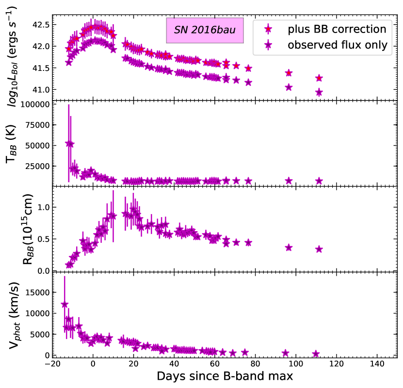
Figure 3.9: The top panel shows the bolometric and quasi-bolometric light curves of SN 2016bau. Second panel: the temperature evolution of SN 2016bau. Third and fourth panels: the radius and velocity evolution (respectively) obtained using blackbody fits.

From the prior knowledge of explosion epoch and radii at various epochs, we estimate the photospheric velocity evolution of this SN in the same way as for SN 2015ap. The bottom panel of Figure 3.9 shows the velocity evolution of SN 2016bau.

From the prior knowledge of $t_{\rm exp}$, a rise time ($t_{\rm rise}$) of 17.09$\pm$1.29 d is obtained. The photospheric velocity near maximum light is $\sim$ 5000 km s^-1, obtained from a blackbody fit. With the known values of $t_{\rm rise}$, the photospheric velocity near maximum light, and a constant opacity ($\kappa$) 0.07 cm² g^-1, we obtain the ejecta mass ($M_{\rm ej}$) and kinetic energy ($E_{\rm ke}$) following Eq. (1) and Eq. (3) of Wheeler et al. (2015); the results are 1.6$\pm$ 0.3 M_⊙ and (0.24$\pm$0.04)$\times$ 10⁵¹ erg, respectively. Following Prentice et al. (2016), an amount of 0.055$\pm$0.006 M_⊙ of ⁵⁶Ni is synthesised, corresponding to a peak luminosity of (1.19$\pm$0.08)$\times$10⁴² erg s^-1.

3.4 Spectral Properties

In this section, we discuss the spectral features of SN 2015ap and SN 2016bau and further compare their properties with other similar SNe. We modelled the spectra of these two SNe at different epochs using SYN++ (Branch et al., 2007; Thomas et al., 2011) and performed the spectral matching of the 12, 13, and 17 M_⊙ spectral models given by Jerkstrand et al. (2015) with the spectra of SN 2015ap and SN 2016bau at phases around 100 d past explosion. In this section, we also estimate the velocities of various lines present in the spectra, using their absorption troughs.

3.4.1 Spectroscopic nature of SN 2015ap

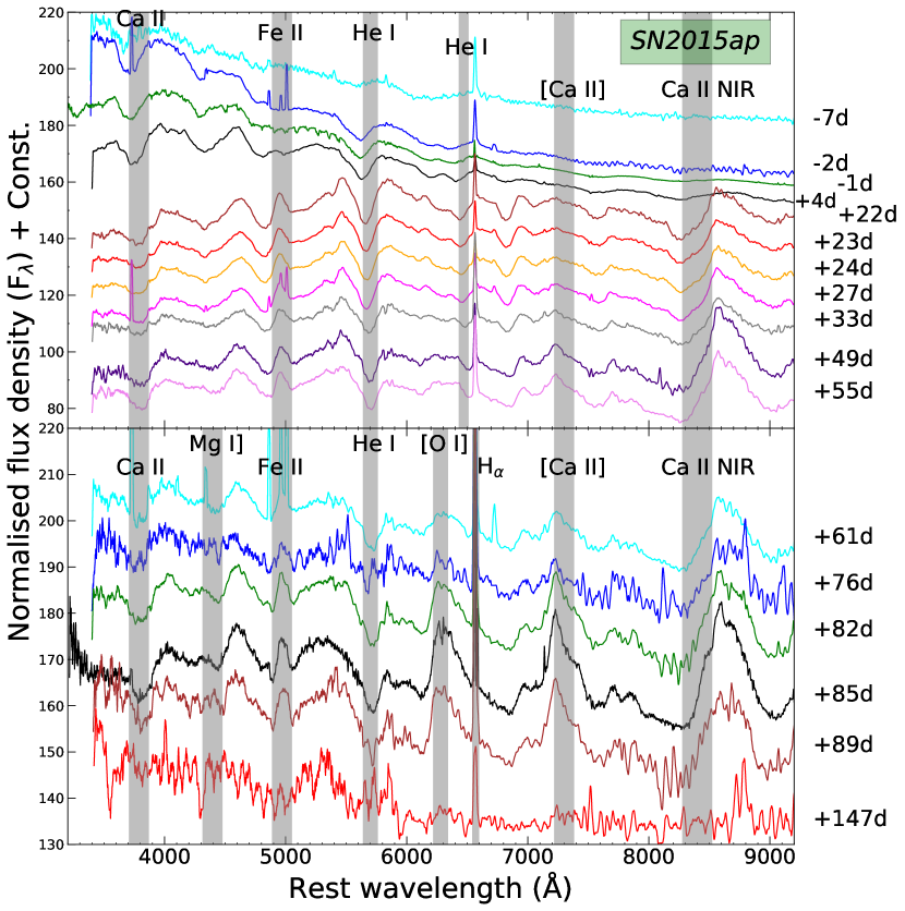
Figure 3.10: Top panel: the early-phase spectra up to +55 d. Bottom panel: the spectral evolution beyond +55 d since $B_{\rm max}$ of SN 2015ap.

The top and bottom panels of Figure 3.10 show the early phases (-7 d to +55 d) and late phases (+61 d to +147 d) spectral evolution, respectively. It is quite evident from the top panel of Figure 3.10 that initially SN 2015ap shows broad-lined features (at -7 d and -2 d), which later evolve to spectra of a normal Type Ib SN. The characteristic He I line at 5876 Å  of a typical SN Ib is clearly seen in the spectra of SN 2015ap. We also see unambiguous He I features at 6678 Å  and 7065 Å, but these two lines are not as prominent as the one at 5876 Å. In the very early phases (up to +4 d), the He I line at 7065 Åis hard to identify. We see that the He I absorption at 5876 Å  is stronger than any other absorption features, and it is present in every spectrum up to +147 d. The Fe II feature near 5169 Å  is very hard to be identified, and it seems to be highly blended with He I 5016 Å.

The spectral evolution also shows the Ca II near-infrared (NIR) feature, which is almost absent in the very early phases (-7 d to +4 d), but starts to develop very strongly from +22 d onward. It is so strong that each spectrum on and after +22 d shows it, even the lowest-SNR spectrum at +147 d. The forbidden [Ca II] feature near 7300 Å  is almost absent at very early phases (-7 d to +4 d), then begins to develop very obviously in the spectra from +22 d, and is present up to +89 d. This [Ca II] feature can also get blended with [O II] emission at 7320 Å  and 7330 Å. It almost disappears in the spectrum at +147 d, though its absence may not be real owing to the very poor SNR of that spectrum. We also see the Ca II H&K feature near 3934 Å, which is present in every spectrum. From the bottom panel of Figure 3.10, we see that as the spectra evolve, the absorption features of different lines tend to disappear and the emission features become more prominent. We see a very weak semiforbidden Mg I] line, at 4571 Å. However, we can clearly see the forbidden emission lines of [O I] and [Ca II], which indicates the onset of the nebular phase.

$\bullet$ Spectral comparison

To investigate the spectroscopic behaviour of SN 2015ap, we compare its spectral features with those of other well-studied SNe Ib such as SN 2004gq (Modjaz et al., 2014), SN 2008D (Modjaz et al., 2014), SN 2012au (Pandey et al., 2021), SN 2009jf (Sahu et al., 2011; Modjaz et al., 2014), iPTF13bvn (Srivastav et al., 2014), SN 2007uy (Modjaz et al., 2014; Milisavljevic et al., 2010), SN 2007gr (Valenti et al., 2008b; Modjaz et al., 2014), and SN 2005bf (Modjaz et al., 2014).

The top panel of Figure 3.11 shows the early phase (-7 d) spectral comparison of SN 2015ap with these well-studied SNe Ib. The spectral features of SN 2015ap look similar to those of SN 2008D and SN 2012au, compared to other SNe Ib. We can see that the Ca II H&K feature, the Mg II feature, and the He I P Cygni profile match very well with those of SN 2008D, while in other SNe in the comparison sample, these features are much more developed. The blue end of the spectrum matches nicely with SN 2008D, while the redder part is featureless and much closer to SN 2012au and SN 2005bf. The He I 5876 Å  feature of SN 2015ap is completely different from that of SN 2007uy, but resembles that of SN 2008D and seems to be less evolved compared to that of SN 2004gq, SN 2012au, SN 2009jf, and iptf13bvn. The Fe II profile in SN 2015ap is hard to detect, which may be due to a very high initial optical opacity. We try to estimate the velocities using the various absorption features. As the spectrum at this epoch is continuum dominated, only a few absorption features were visible. The velocity estimated using He I absorption lines is $\sim$ 14,100 km s^-1.

Figure 3.11: Spectral comparison of the spectra of SN 2015ap and SN 2016bau at epochs -7 d (top panel), +33 d (middle panel), and +61 d (bottom panel). Various important SN Ib features have been compared with those of other similar-type SNe.

Further, we compare the +33 d spectrum of SN 2015ap with our comparison sample (middle panel of Figure 3.11). At this epoch, the spectrum of SN 2015ap shows various P Cygni profiles. We see that it almost exactly replicates the +22 d spectrum of SN 2008D. The blended He I and Fe II profiles near 5016 Å  well match those of other SNe Ib, except for SN 2007uy, where the peak is almost absent, and for SN 2005bf, where it is double-peaked. The He I feature at 5876 Å  matches well with other SNe Ib except for the cases of SN 2007uy and SN 2005bf, where the absorption features seem to be much broader. Here, once again, SN 2007uy seems to match much less and SN 2008D seems to best match the +22 d spectrum of SN 2015ap. The velocities estimated using the Ca II NIR triplet and He I absorption features are $\sim$ 7800 km s^-1 and 10000 km s^-1, respectively.

For a much clear comparison, we compared the +61 d spectrum of SN 2015ap (bottom panel of Fig. 3.11) with spectra of other well-studied SNe Ib. At this epoch also, the spectrum is still much closer to that of SN 2008D compared to other SNe Ib. The blended Fe II and He I features near 5016 Å  show an almost similar profile to that of SN 2008D. However, the 5876 Å  He I profile is narrower in SN 2015ap compared to SN 2008D. We can see the onset of the appearance of the [O I] line in SN 2015ap, which differs from SN 2008D. The He I profile is well matched in the cases of SN 1999dn and SN 2009jf, but the Ca II NIR triplet of these SNe differs from that of SN 2015ap. Here the velocities estimated using the Ca II NIR triplet and He I absorption features are $\sim$ 6900 km s^-1 and 8100  km s^-1, respectively.

$\bullet$ Spectral modelling

After confidently identifying the features present in the spectra of SN 2015ap and comparing them with those of other well-studied SNe, we tried to model a few spectra at various epochs using SYN++. The top panel in Figure 3.12 shows the early-phase (-7 d) spectrum of SN 2015ap. This spectrum displays weak and broad P Cygni profiles of He I, Ca II H&K, and the Ca II NIR triplet, and also some blended features of Fe II. We also show the best-matching synthetic spectrum, generated by SYN++. The absorption features due to Ca II H&K, Ca II NIR triplet, He I, and Fe II multiplets are easily reproduced. The photospheric velocity and blackbody temperature associated with the best-fit spectrum are 12,000 km s^-1 and 12,000 K, respectively. We perform SYN++ matching to four additional spectra from epochs -2 d to +33 d (Fig. 3.12). With the passage of time, the SN expands, cools gradually, and its expansion velocity decreases slowly, so we see a gradual decrease in the values of these fitted parameters. The photospheric velocities during the phase of -7 d to +33 d vary from 13,000 km s^-1 to 6800 km s^-1, and the blackbody temperature varies from 12,000 K to 4500 K, which are in good agreement with those obtained photometrically from blackbody fits. Owing to the local thermodynamic equilibrium (LTE) approximation, SYN++ does not work well for the later epochs and cannot be used to fit the spectra.

To get an estimate of the progenitor mass, we used the +98.75 d post-explosion spectrum of SN 2015ap and plotted it along with the 12, 13, and 17 M_⊙ model spectra from Jerkstrand et al. (2015) at 100 d, after scaling by a factor of exp$(-2\times\Delta t/111.4)$ (Jerkstrand et al., 2015), where $\Delta t$ = 1.25, is the time difference between the epoch of the model spectrum and the epoch of the observed spectrum. We can see that the 12 M_⊙ and 17 M_⊙ model spectra seem to reproduce the observed spectrum of SN 2015ap. The 12 M_⊙ spectrum very nicely matches the observed spectrum throughout the entire wavelength range, while the 17 M_⊙ spectrum slightly overproduces the flux near the Ca II NIR triplet close to 8500 Å. However, the 13 M_⊙ model spectrum fails to explain the observed fluxes throughout the entire wavelength range. Thus, based on this analysis, a range of 12–17 M_⊙ is expected for the possible progenitor mass of SN 2015ap, in agreement with that described by Gangopadhyay et al. (2020).

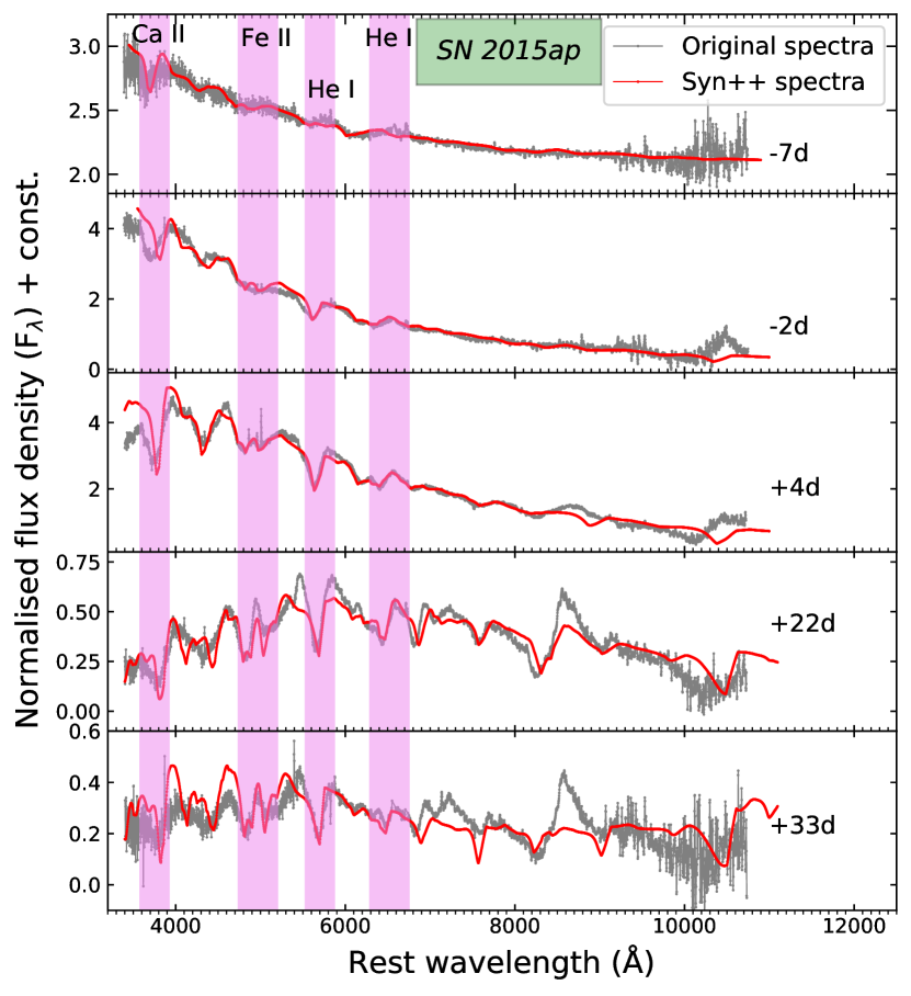
Figure 3.12: SYN++ modelling of the spectra of SN 2015ap at epochs -7 d, -2 d, +4 d, +22 d, and +33 d. Prominent He I features could be produced nicely.

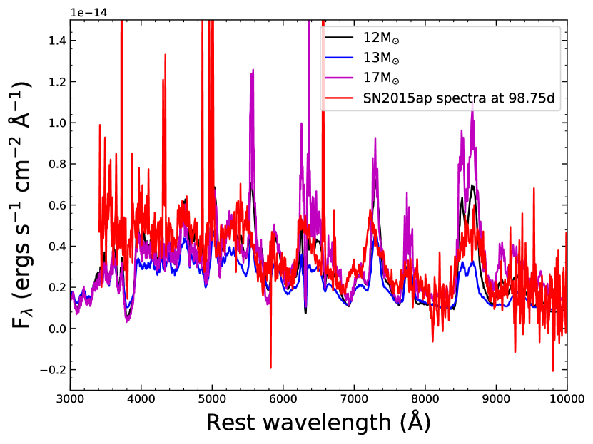
Figure 3.13: The $t=$+98.75 d spectrum of SN 2015ap plotted along with the 12, 13, and 17 M_⊙ models from Jerkstrand et al. (2015) at 100 d scaled with an exponential factor exp$(-2\times 1.25/111.4)$. The 12 M_⊙ and 17 M_⊙ models seem to best match the observed spectrum of SN 2015ap.

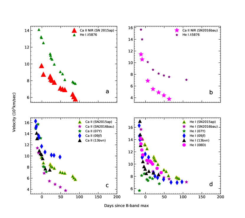
Figure 3.14: (a) The temporal evolution of velocities of He I 5876 Å  and the Ca II NIR triplet for SN 2015ap. (b) Same as (a) but for SN 2016bau. The bottom two panels show the comparison of these line velocities of SN 2015ap and SN 2016bau with SNe 2007Y (Stritzinger et al., 2009), 2009jf (Sahu et al., 2011), iPTF13bvn (Srivastav et al., 2014), and 2008D (Modjaz et al., 2014).

$\bullet$ Velocity evolution of various lines of SN 2015ap

We used the blue-shifted absorption minima of P Cygni profiles and the special-relativistic Doppler formula (Sher, 1968) to obtain the velocities of several lines. Figure 3.14$a$ shows the He I and the Ca II NIR triplet velocity evolution of SN 2015ap. In the initial few days, the line velocities tend to decrease rapidly. At an epoch of +24 d, the velocities estimated using He I 5876 Å  and the Ca II NIR triplet are $\sim$ 10,600 km s^-1 and 8200 km s^-1, respectively. The velocities estimated using these two lines drop to $\sim$ 9100 km s^-1 and 7100 km s^-1 (respectively) at an epoch of +49 d. In the late phases, the velocities decline gradually.

Figure 3.14$c,d$, show comparisons of velocities obtained using the Ca II NIR triplet and He I 5876 Å  features with other well-studied SNe. Initially the Ca II NIR line velocity of SN 2015ap evolves in a manner similar to iptf13bvn, thereafter it decays slowly, attaining a velocity of $\sim$ 7600 km s^-1 at +89 d. We see that the ejecta velocity of SN 2015ap obtained using He I 5876 Å  is higher than that of other SNe Ib but closer to SN 2008D.

3.4.2 Spectral properties of SN 2016bau

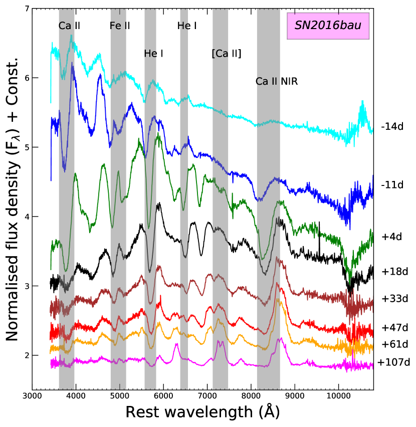
Figure 3.15: Various line identifications in the overall spectral evolution of SN 2016bau. Strong He I features along with other important lines are indicated.

Figure 3.15 shows the spectral evolution of SN 2016bau for a period of -14 d to +107 d. In the first spectrum (-14 d), we see well-developed He I features (5876, 6678, and 7065 Å). Also, the spectrum on this particular epoch displays a weak and broad Ca II NIR feature, but with the passage of time (beyond $\sim$+33 d), prominent Ca II NIR features start to appear. We also see that in the initial phases, there is a strong Ca II H $\&$ K feature, but it becomes progressively weaker in later phases. As the phase approaches the date of $B$-band maximum brightness, the He I features start to appear much more strongly, as seen in the spectra at -11 d, +4 d, and +18 d. Beyond $-11$ d, the longer wavelengths exhibit strong Ca II NIR features. The spectra also display very strong P Cygni profiles of He I at 5016 Å  after $t=$ -11 d. The emergence of very strong features of He I in the early-time spectra confirms this SN to be of Type Ib.

$\bullet$ Spectral comparison

To investigate the spectroscopic behaviour of SN 2016bau, we have compared its spectral features with those of other well-studied SNe Ib. We used a sample similar to that for SN 2015ap. The top panel of Figure 3.11 shows the early-phase (-11 d) spectral comparison of SN 2016bau with other well-studied H-stripped CCSNe. The spectral features of SN 2016bau look much more similar to those of SN 2012au, SN 2009jf, and SN 1999dn compared to other SNe. we can see that the Ca II  H&K feature, the Mg II feature, and the He I P Cygni profile of SN 2016bau match very well those of SN 2012au, SN 2009jf, and SN 1999dn. The He I 5876 Å  feature of SN 2016bau is completely different from that of SN 2007uy, SN 2015ap, and SN 2008D. As with SN 2015ap, the blended Fe II profile in SN 2016bau is hard to detect, which may be due to a very high initial optical opacity. The spectrum at this epoch has nicely developed He I features. The velocity estimated using the He I 5876 Å  absorption line is $\sim$ 15,600 km s^-1.

The middle panel of Figure 3.11 shows the +33 d spectral comparison of SN 2016bau with other well-studied SNe Ib. The spectrum at this epoch contains many P Cygni profiles of various lines. These spectral features look most similar to those of SN 2008D and SN 2015ap, compared to other SNe Ib. We see that the Ca II NIR feature, the Fe II feature, and the He I P Cygni profile match very well those of SN 2008D and SN 2015ap, compared to other SNe. SN 2009jf also seems to match nicely in the redder part of the spectrum. The He I 5876 Å  feature of SN 2016bau is completely different from those of SN 2007uy, SN 2005bf, SN 2004gq, and SN 2007gr, but resembles those of SN 2008D, SN 2015ap, and SN 2009jf. The He I 5876 Å  profile of SN 2016bau seems to be more asymmetric and narrower than that of iptf13bvn. At this epoch, the velocities estimated using the absorption features of He I and the Ca II NIR triplet are $\sim$ 8100 km s^-1 and 4900 km s^-1, respectively.

For much clearer comparisons, we also compared the +61 d spectrum of SN 2016bau (bottom panel of Figure. 3.11) with other well-studied H-stripped CCSNe spectra. At this epoch, the bluer part of the spectrum is much closer to SN 2008D compared to other SNe Ib. Here the blended Fe II and He I feature near 5016 Å  shows a nearly similar profile to those of SN 2008D and SN 2009jf. However, the 5876 Å  He I profile is broader in SN 2016bau compared with SN 2008D. We can see that the onset of the appearance of [O I] in SN 2016bau is slightly different from that of SN 2008D, while it matches nicely that of SN 2009jf. The He I profile is well matched in the case of SN 2008D. Here the velocities estimated using the Ca II NIR and He I absorption features are $\sim$ 3700 km s^-1 and 7600 km s^-1, respectively.

$\bullet$ Spectral modelling

After confidently identifying various spectral features, we tried to model the spectra of SN 2016bau at different epochs using SYN++. The top panel of Figure 3.16 shows the early-phase (-14 d) spectrum of SN 2016bau. It contains many broad P Cygni profiles of He I, Ca II H&K, the Ca II NIR triplet, and also some blended features of Fe II. In this figure, we have also presented the best-matching synthetic spectrum generated by SYN++. The modelled spectrum easily reproduces the absorption features of Ca II H&K, Ca II NIR, He I, and the Fe II multiplet. The photospheric velocity and blackbody temperature associated with the best-fit spectrum are 16,000 km s^-1 and 9000 K respectively. We performed SYN++ matching for four additional spectra which covers a period of -11 d to +33 d (subsequent panels of Fig. 3.16). With the passage of time, the SN expands and cools gradually, and its expansion velocity decreases slowly, so we see a gradual decrease in the fit parameters such as velocity and temperature in the later phases. The photospheric velocity during the phase of -14 d to +33 d varies from 16,000 km s^-1 to 8000 km s^-1 and the blackbody temperature ranges from 9000 K to 4000 K, in good agreement with values obtained photometrically from blackbody fits.

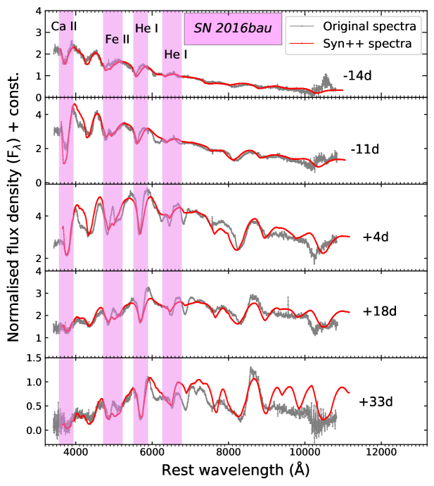
Figure 3.16: SYN++ modelling of the spectra of SN 2016bau at epochs -14 d, -11 d, +4 d, +18 d, and +33 d.

We also try to match the +121 d spectrum of SN 2016bau with the 12 M_⊙, 13 M_⊙, and 17 M_⊙ model spectra at +100 d from Jerkstrand et al. (2015), scaled with a factor of exp$(-2\times\Delta t/111.4)$ (Jerkstrand et al., 2015), where $\Delta t$ = 21, is the time difference of the epoch of model spectrum and the epoch of observed spectrum. We can see that all three models over–predict the observed fluxes from 3000 Å  to around 6000 Å, beyond which the 12 M_⊙ model spectrum seems to best describe the observed spectrum. It could nicely explain the [Ca II] emission near 7300 Å  and the Ca II NIR feature near 8500 Å. The 13 M_⊙ model spectrum also produces the [Ca II] emission but fails to explain the observed fluxes near the Ca II-NIR triplet. The 17 M_⊙ model spectrum overpredicts the flux throughout the entire wavelength range and thus fails to explain the spectrum of SN 2016bau. Hence, based on our analysis, a slightly low-mass progenitor ($\leq$12 M_⊙) is expected.

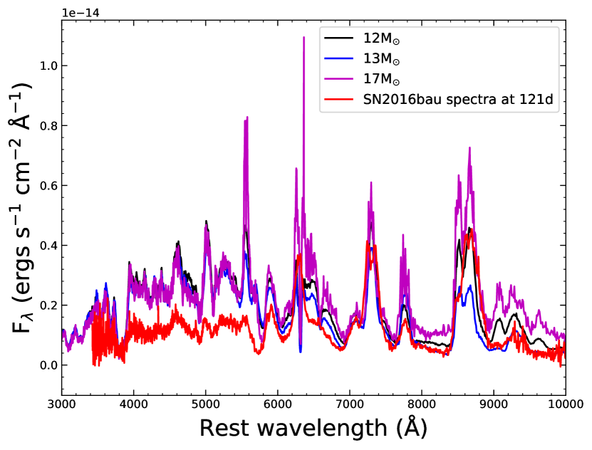
Figure 3.17: The $t=$+121 d spectrum of SN 2016bau plotted along with the 12, 13, and 17 M_⊙ models from Jerkstrand et al. (2015) at 100 d scaled with an exponential factor exp$(-2\times 21/111.4)$. The 12 M_⊙ model seems to best match the spectrum of SN 2016bau.

$\bullet$ Velocity evolution of Various lines of SN 2016bau

We used the blue-shifted absorption minima of P Cygni profiles to obtain the velocities of He I and Ca II NIR lines. Figure 3.14$b$ shows the He I and Ca II NIR velocity evolution of SN 2016bau. In the initial few days, the line velocities tend to decrease rapidly, but in later phases, the velocities decline gradually. At an early epoch of -14 d, the velocities estimated using He I 5876 Å  and the Ca II NIR triplet are $\sim$ 15,600 km s^-1 and $\sim$ 11,400 km s^-1, respectively. The velocities estimated using these two lines drop to $\sim$ 7800 km s^-1 and $\sim$ 4400 km s^-1 (respectively) at an epoch of +47 d. Beyond +47 d, the velocities continue to decline at a slower rate as compared to the initial decline rate. Figure 3.14$c,d$ show the comparison of these two line velocities with other well-studied SNe. Initially, the Ca II NIR velocity declines very fast but in the later epochs, only a gradual decline is seen. It evolves in a manner very similar to iPTF13bvn, but in the late phases, the velocities are slower than other SNe. The velocities obtained using He I 5876 Å of SN 2016bau evolve in a manner similar to that of other SNe Ib, but much closer to SN 2009jf and iPTF13bvn. The He I line velocity of SN 2016bau at +33 d reaches $\sim$ 8200 km s^-1, nearly equal to those of SN 2009jf and iPTF13bvn.

3.5 Fitting the Multi-band Light Curves using MOSFiT

MOSFiT(Guillochon et al., 2018) is a Python-based package that downloads data from openly available online catalogues, generates the Monte Carlo ensembles of semi-analytical light curve fits to the downloaded data sets along with their associated Bayesian parameter posteriors and provides the fitting results back. Besides fitting data downloaded from openly available online catalogues, one can also perform a similar analysis to the private data sets. MOSFiT employs various powering mechanisms for the light curves of different types of SNe. Some of them are; a) default model incorporating the Nickel-Cobalt decay (Nadyozhin, 1994), b) magnetar model that takes a magnetar engine with simple spectral energy distribution (Nicholl et al., 2017), and c) csm model which is interacting CSM–SNe (Chatzopoulos et al., 2013; Villar et al., 2017). A detailed description of all the models available through MOSFiT is provided in Guillochon et al. (2018).

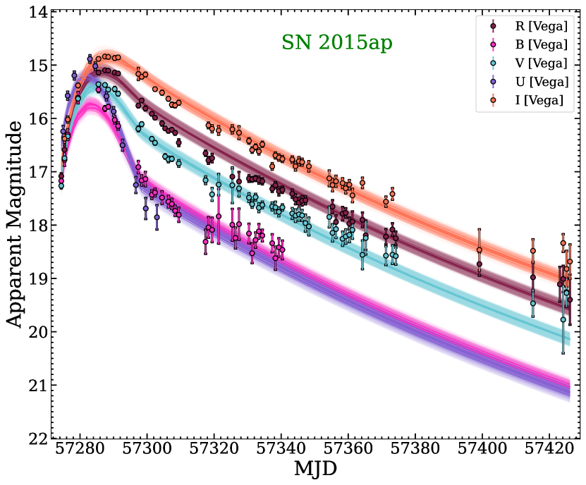
Figure 3.18: The results of MOSFiT fittings to the multi band light curves of SN 2015ap. For Type Ib SNe, the radioactive decay of nickel and cobalt is considered to be the prominent powering mechanism for their light curves. Thus, the default model from MOSFiT has been employed to fit the light curves.

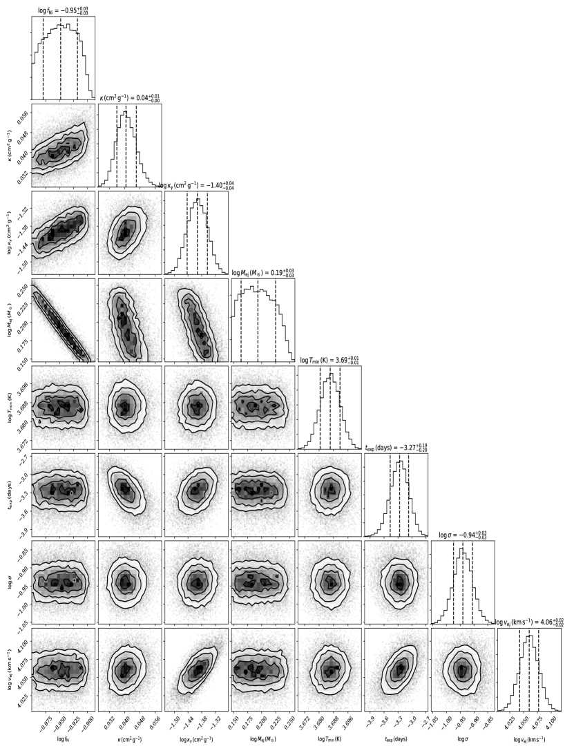
Figure 3.19: The corner plot of the fitting parameters from the default model for SN 2015ap using MOSFiT.

$\bullet$  For SN 2015ap: The default model incorporating the Nickel-Cobalt decay is considered the prominent powering mechanism for the Type Ib SNe. Thus, we tried to fit the multi-band light curves of SN 2015ap utilising the default model. The multi-band light curves were corrected for total extinction (host galaxy plus Milky Way). The results of MOSFiT fittings utilising the default models are displayed in Figure 3.18. A corresponding corner plot is also shown in Figure 3.19. The ejecta mass obtained through MOSFiT fitting is $\sim$1.5 M_⊙ which is close to the value obtained by Prentice et al. (2019). The detailed fitting parameters are tabulated in 3.1.

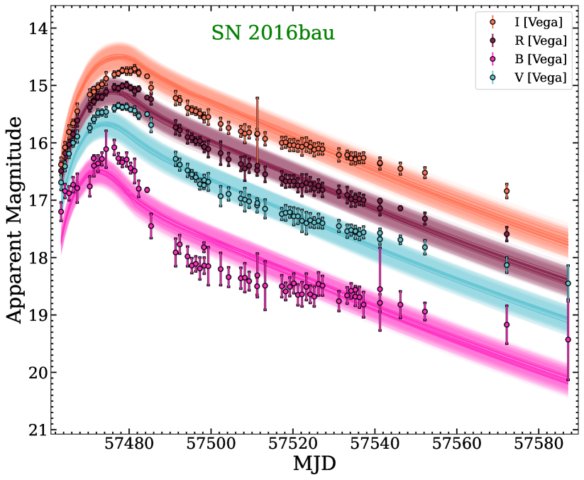
Figure 3.20: The results of MOSFiT fittings to the multi band light curves of SN 2015ap. For Type Ib SNe, the radioactive decay of nickel and cobalt is considered to be the prominent powering mechanism for their light curves. Thus, the default model from MOSFiT has been employed to fit the light curves.

Source name	$\log\,M_{\rm ej}$ (M${}_{\odot})$	$\log\,f_{\rm Ni}$	$\kappa\,({\rm cm}^{2}\,{\rm g}^{-1})$	$\log\,\kappa_{\gamma}\,({\rm cm}^{2}\,{\rm g}^{-1})$	$\log\,v_{\rm ej}\,({\rm km\,s}^{-1})$	$\log\,T_{\min}\,{\rm(K)}$	$\log\,\sigma$	$t_{\rm exp}\,{\rm(days)}$
SN2015ap	0.19${}_{-0.03}^{+0.03}$	-0.95${}_{+0.03}^{-0.03}$	0.04${}_{-0.00}^{+0.01}$	-1.40${}_{-0.04}^{+0.04}$	4.06${}_{-0.02}^{+0.02}$	3.69${}_{-0.01}^{+0.01}$	-0.94${}_{+0.03}^{-0.03}$	-3.27${}_{+0.19}^{-0.20}$
SN2015ap∗	0.25${}_{-0.12}^{+0.16}$	-0.24${}_{+0.15}^{-0.22}$	0.10${}_{-0.03}^{+0.05}$	1.73${}_{-1.58}^{+1.48}$	4.45${}_{-0.03}^{+0.03}$	3.41${}_{-0.25}^{+0.24}$	-0.80${}_{+0.07}^{-0.05}$	-3.64${}_{+0.29}^{-0.40}$
SN2016bau	0.19${}_{+0.02}^{-0.01}$	-0.94${}_{+0.02}^{-0.02}$	0.05${}_{-0.00}^{+0.00}$	-1.46${}_{-0.06}^{+0.06}$	3.95${}_{-0.02}^{+0.02}$	3.82${}_{-0.01}^{+0.01}$	-0.65${}_{+0.02}^{-0.02}$	-4.88${}_{+0.14}^{-0.06}$
SN2016bau∗	-0.51${}_{+0.23}^{-0.18}$	-1.01${}_{+0.21}^{-0.25}$	0.10${}_{-0.03}^{+0.04}$	2.45${}_{-3.41}^{-2.48}$	3.58${}_{-0.02}^{+0.14}$	3.55${}_{-0.38}^{+0.31}$	-1.72${}_{+0.23}^{-0.18}$	-4.41${}_{+0.29}^{-0.36}$

Table 3.1: Best-fit parameters and 68 % uncertainties for the default model. The parameters for the source with * are the results from Meyer et al. (2020) presented here for comparison with our studies. In this table, $M_{ej}$ is the ejecta mass, $f_{Ni}$ is the nickel mass fraction, $\kappa$ is the Thomson electron scattering opacity, $\kappa_{\gamma}$ is gamma-ray opacity of the SN ejecta, $v_{ej}$ represents the ejecta velocity, $T_{min}$ is an additional parameter for temperature floor [ please see Nicholl et al. (2017), for further details ], $\sigma$ is an additional variance parameter which is added to each uncertainty of the measured magnitude so that the reduced $\chi^{2}$ approaches 1, and $t_{\rm exp}$ is the epoch of explosion since first detection.

$\bullet$  For SN 2016bau: Similar to SN 2015ap, the default model is employed for the multi-band light curves of SN 2016bau after correcting for the total extinction. The fitting results are displayed in Figure 3.20. The detailed fitting parameters are tabulated in Table 3.1.

3.6 MINIM Modelling of the Quasi-bolometric Light Curve

In this section, we fit the radioactive decay (RD) and the magnetar (MAG) powering mechanisms, as discussed by Chatzopoulos et al. 2013 (see also Wheeler et al. 2017; Kumar et al. 2020, 2021), by employing the MINIM (Chatzopoulos et al., 2013) code. MINIM is a $\chi^{2}$-minimisation fitting code that utilises the Price algorithm (Brachetti et al., 1997). In the RD model, the radioactive decay of ⁵⁶Ni and ⁵⁶Co leads to the deposition of energetic gamma-rays that are assumed to thermalise in the homologously expanding SN ejecta and thus powering the light curve. In the MAG model, the light curves are powered by the energy released by the spin-down of a young magnetar located in the centre of the SN ejecta. Following Prentice et al. (2019), we have adopted a constant opacity, $\kappa$ = 0.07 cm² g^-1, for both SN 2015ap and SN 2016bau.

3.6.1 SN 2015ap

Figure 3.21 shows the results of RD and MAG model fittings to the quasi-bolometric light curve of SN 2015ap. The fitted and calculated parameters are listed in Tables 3.2 and 3.3. The ejecta mass ($M_{\rm ej}$) in the RD and MAG models was calculated using Eq. 1 from Wheeler et al. (2015). Although the RD model seems to reasonably fit the observed quasi-bolometric light curve, it seems unable to reproduce not only the observed peak luminosity but also the light curve at late phases, after +50 d. The nickel mass and ejecta mass obtained from these models are somewhat smaller than the ones inferred directly from the observed rise time and peak luminosity in Sec.3.5. As the RD model is the prominent powering mechanism for normal SNe Ib, we tried to fit the RD model only up to a relatively early phase ($\sim$ +20 d). In the inset of Figure 3.21, we see that the early phase is nicely fitted in this case. A nickel mass ($M_{\rm Ni}$) of 0.181$\pm$ 0.006 M_⊙ and an ejecta mass ($M_{\rm ej}$) of 2.1$\pm$0.09 M_⊙ obtained through this fitting are close to the observed values listed in Sec.3.5. The fitted and calculated values from the photospheric phase are collected in Table 3.2.

The MAG model fits the whole observed light curve, both around peak brightness as well as during the late phase, better than the RD model. However, the fitted parameters seem to be unphysical, particularly the very slow initial rotation ($P_{i}\approx$40 ms) and the very low initial rotational energy ($E_{p}\approx$10⁴⁹ erg). This is not surprising given that the magnetar model contains two timescales, one for the rising part and another for the declining part of the light curve (Chatzopoulos et al., 2013). Thus, the possibility of SN 2015ap powered by spin-down of a magnetar is less likely.

Table 3.2: Minimum $\chi^{2}$/dof parameters for SN 2015ap and SN 2016bau for the RD model.

	$M_{\mathrm{Ni}}$a	$t_{\mathrm{d}}$b	$A_{\mathrm{\gamma}}$c	$M_{\mathrm{ej}}$b	$\chi^{2}/\mathrm{dof}$
	(M⊙)	(days)		(M⊙)
SN 2015ap
whole light curve	0.094 $\pm$ 0.004	8.0 $\pm$ 2.0	30.05 $\pm$ 1.05	0.64 $\pm$ 0.3	6.2
+20 d data	0.181 $\pm$ 0.006	14.5 $\pm$ 0.3	5.3 $\pm$ 0.3	2.1 $\pm$ 0.09	1.2
SN 2016bau
whole light curve	0.08 $\pm$ 0.01	20.5 $\pm$ 0.7	7.8 $\pm$ 0.5	2.8 $\pm$ 0.2	22.7
+20 d data	0.065 $\pm$ 0.001	18.09 $\pm$ 0.3	9.95 $\pm$ 0.4	1.81 $\pm$ 0.07	1.2

$a$, mass of ⁵⁶Ni synthesised; $b$, effective diffusion timescale; $c$, optical depth for the $\gamma$-rays measured 10 d after the explosion; $d$, ejecta mass, with $\kappa=$0.07 cm² g^-1.

3.6.2 SN 2016bau

Figure 3.22 shows the results of the RD and MAG model fittings to the quasi-bolometric light curve of SN 2016bau. The fitted and calculated parameters are listed in Tables 3.2 and 3.3. The RD model can fit the observed peak luminosity, but huge deviations from the observed light curve are seen in the later phases. The model also fails to match the observed stretch factor of the light curve. Like SN 2015ap, we also tried to fit only the early part, before +20 d post-peak (see the inset in Fig. 3.22). In this case, the fitted parameters, such as the nickel mass of 0.065$\pm$0.002 M_⊙ and the ejecta mass of 1.81$\pm$0.07 M_⊙ (see Table 3.2), are very close to the observed values in Section 3.8. Similar to SN 2015ap, the slow rotation ($P_{i}\approx$70 ms), low magnetar rotational energy ($E_{p}\approx$10⁴⁸ erg), and very high progenitor radius ($\sim$ 1200 R_⊙) make the MAG model physically unrealistic for SN 2016bau, despite the better fit to the whole light curve in Figure 3.22.

Table 3.3: Minimum $\chi^{2}$/dof parameters for SN 2015ap and SN 2016bau for the MAG model.

	$R_{0}$a	$E_{p}$b	$t_{d}$c	$t_{p}$d	$v_{\rm exp}$e	$M_{\rm ej}$f	$P_{i}$g	$B$h	$\chi^{2}/\mathrm{dof}$
	($10^{13}$ cm)	($10^{51}$ erg)	(days)	(days)	($10^{3}$ km s-1)	(M⊙)	(ms)	($10^{14}$ G)
SN 2015ap
	0.594 $\pm$ 0.003	0.01210 $\pm$ 0.00007	8.7 $\pm$ 0.1	12.06 $\pm$ 0.08	6.03 $\pm$ 0.02	0.75$\pm$ 0.02	40.6 $\pm$0.1	25.5$\pm$ 0.2	1.54
SN 2016bau
	7.9 $\pm$ 0.7	0.00403 $\pm$ 0.00007	8.5 $\pm$ 0.1	15.1 $\pm$ 0.1	6.2 $\pm$ 0.5	1.26$\pm$ 0.02	70.4$\pm$ 0.6	52.6$\pm$ 0.8	1.4

$a$, progenitor radius; $b$, magnetar rotational energy; $c$, effective diffusion timescale (in days); $d$, magnetar spin-down timescale; $e$, SN expansion velocity; $f$, $\kappa=$0.07 cm² g^-1 is used; $g$, initial period of the magnetar; $h$, magnetic field of the magnetar.

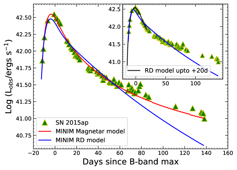
Figure 3.21: MINIM modelling of the quasi-bolometric light curve of SN 2015ap. The inset shows the RD model fitting only for the early phase (up to +20 d).

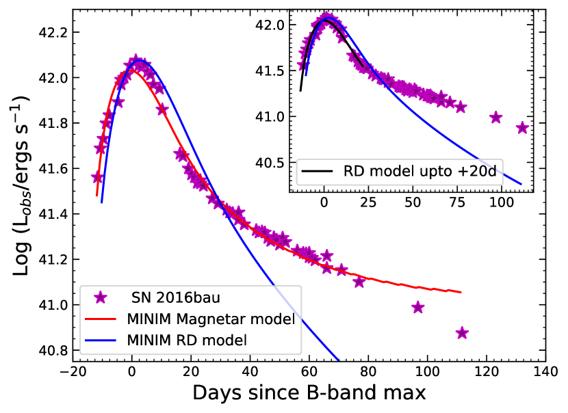
Figure 3.22: MINIM modelling of the quasi-bolometric light curve of SN 2016bau. The figure in the inset shows the RD model fitting only for the early phase (up to +20 d).

3.6.3 Summary of MINIM modelling

The failure of the semi-analytical RD models to simultaneously fit the early and late parts of the light curves of SN 2015ap and SN 2016bau highlights the issues related to the validity of such kinds of models in the case of stripped-envelope SNe. The difficulty in explaining the late-phase decline rate with the assumed diffusion model has already been explored by Wheeler et al. (2015).

Figures 3.21 and 3.22 reveal another issue: the model light curve is steeper after +30–40 d than the observed one. This indicates that the early- and late-phase data cannot be fitted simultaneously with the same model parameters. Even though the nickel mass of the second model fits (insets in Figs. 3.21 and 3.22) the observed peak luminosity, the decline rate, which is related to the ejecta mass (as in Eq. 1 of Wheeler et al. 2015) is clearly too fast, suggesting an underestimated $M_{\rm ej}$.

This issue is very probably related to the assumption of the constant ejecta density profile (and also the constant opacity). The less steep late part of the light curve needs more ejecta mass to trap the heating gamma-rays originating from the Ni and Co decay. The early part, however, suggests ejecta that dilute much faster than what can fit the late part. Within the context of the constant-density model, this dichotomy means that fitting only the early part results in a lower ejecta mass compared to fitting only the late part (Figure 3.23).

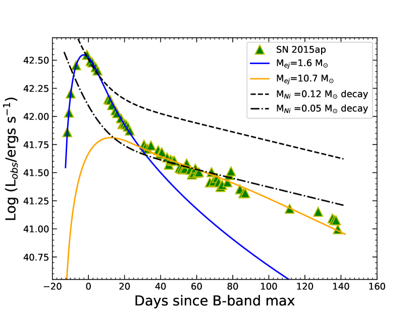
Figure 3.23: Detailed MINIM modelling to the quasi-bolometric light curve of SN 2015ap. All of the models with different $M_{\rm ej}$ and $M_{\rm Ni}$ are shown together. The models with $M_{\rm ej}=$1.6 M_⊙ and 10.7 M_⊙ show the RD model fittings considering only the early- and late-phase data, respectively. The other two models show the effect of the amount of nickel present.

Since this issue cannot be solved self-consistently with the constant-density model, and it can plague the mass estimates that consider only the early or late part of the light curve, we investigate it further in the following sections by applying more realistic models for the progenitors and the SN light curves.

3.7 MESA Modelling of a 12 M_⊙ ZAMS Progenitor Star

Adoption of a 12 M_⊙ ZAMS progenitor star for SN 2015ap is primarily based on the results of comparison of the three models from Jerkstrand et al. (2015) and also in the literature; in addition, it supports the observed amount of ejecta mass for SN 2015ap. The ejecta mass for SN 2016bau was calculated to be $\sim$ 1.6 M_⊙. On account of such an ejecta mass and the result of Jerkstrand et al. (2015) spectral model matching, we also choose a 12 M_⊙ ZAMS star as a possible progenitor for SN 2016bau.

We first evolve the 12 M_⊙ ZAMS star until the onset of core-collapse, using the 1-dimensional stellar evolution code MESA, version 11701(Paxton et al., 2011, 2013, 2015, 2018). We do not consider rotation and assume an initial metallicity of Z = 0.02. Convection is modelled using the mixing theory of Henyey et al. (1965), adopting the Ledoux criterion. We set the mixing-length parameters to $\alpha$ = 3.0 in the region where the mass fraction of hydrogen is greater than 0.5, and set it to 1.5 in the other regions. Semi-convection is modelled following Langer et al. (1985) with an efficiency parameter of $\alpha_{\mathrm{sc}}$ = 0.01. For the thermohaline mixing, we follow Kippenhahn et al. (1980), and set the efficiency parameter as $\alpha_{\mathrm{th}}$ = 2.0. We model the convective overshooting with the diffusive approach of Herwig (2000), with $f$= 0.01 and $f_{0}$ = 0.004 for all the convective core and shells. We use the ‘Dutch’ scheme for the stellar wind, with a scaling factor of 1.0. The ‘Dutch’ wind scheme in MESA combines results from several papers. Specifically, when $T_{\mathrm{eff}}>$10⁴ K and the surface mass fraction of hydrogen is greater than 0.4, the results of Vink et al. (2001) are used, and when $T_{\mathrm{eff}}>$10⁴ K and the surface mass fraction of hydrogen is less than 0.4, the results of Nugis & Lamers (2000) are used. In the case when $T_{\mathrm{eff}}<$10⁴ K, the de Jager et al. (1988) wind scheme is used.

SNe Ib have been considered to originate from massive stars which lose almost all of their H-envelope, most probably due to binary interaction (e.g., Yoon et al., 2010; Dessart et al., 2012a; Eldridge & Maund, 2016; Ouchi & Maeda, 2017). Here, to produce such a stripped model, we artificially strip the H-envelope, mimicking the binary interaction. Specifically, after evolving the model until the exhaustion of helium, we impose an artificial mass-loss rate of $\dot{M}\gtrsim$10^-4 M_⊙ yr^-1 until the total hydrogen mass of the star goes down to 0.01 M_⊙. After the hydrogen mass reaches the specified limit, we switch off the artificial mass loss and evolve the model until the onset of core collapse. At the time of the core collapse, our model has a total mass of 3.42 M_⊙.

3.8 Synthetic Explosions of Modelled Progenitors Using SNEC and STELLA

In this section we briefly discuss the assumptions and setups to produce artificial explosions using SNEC and STELLA for SN 2015ap and SN 2016bau.

3.8.1 Results of synthetic explosions for SN 2015ap

Using the progenitor model on the verge of core-collapse obtained through MESA, we have conducted the radiation hydrodynamic simulations. For this purpose, we use the publicly available codes SNEC and STELLA.

SNEC is a 1-dimensional Lagrangian hydrodynamic code, which also solves radiation energy transport with the flux-limited diffusion approximation. The code generates the bolometric light curve and the photospheric velocity evolution of the SN, along with a few other observed parameters. The setup for the calculation using SNEC closely follows Ouchi & Maeda (2019). Here, we briefly summarise the important parameters and modifications made to Ouchi & Maeda (2019). First, we excise the innermost 1.4 M_⊙ before the explosion, assuming it collapses to form an NS. The number of cells is set to be 70. Although this number is relatively small, we have confirmed that the SN’s light curve and photospheric velocity are well converged in the time domain of interest. We tried following two possible powering mechanisms for SN 2015ap using SNEC, as follows.

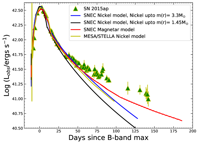
Figure 3.24: Comparison of the quasi-bolometric light curve of SN 2015ap with those obtained using SNEC by considering the Ni–Co decay and the magnetar model. This figure also depicts the result of the Ni–Co decay model obtained using STELLA.

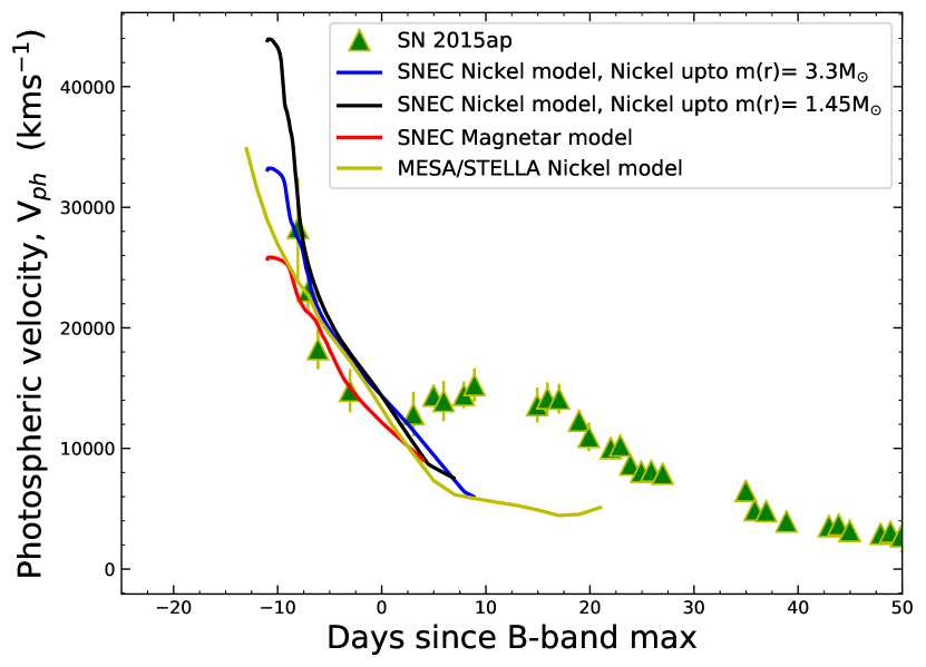
Figure 3.25: Comparison of the observed velocity evolution of SN 2015ap with that produced by SNEC and STELLA for the two models employed.

$\bullet$ Ni–Co decay

The radioactive decay of Ni and Co is considered to be the most prominent mechanism for the powering of light curves of SNe Ib (e.g., Karamehmetoglu et al., 2017b). SNEC incorporates this model by default. Here, we provide the setup of the explosion parameters to incorporate the Ni–Co decay model. The code does not include a nuclear-reaction network, and ⁵⁶Ni is given by hand. We considered two scenarios of nickel distribution. In one case, the mass of Ni is set to be $M_{\mathrm{Ni}}$ = 0.135 M_⊙ and distributed from the inner boundary up to the mass coordinate $m(r)$ = 3.3 M_⊙. For this model, the explosion is simulated as a piston, with the first two computational cells of the profile boosted outward with a velocity of 4.0$\times$10⁹ cm s^-1 for a time interval of 0.01 s. The total energy ($E_{\rm tot}$) of the model is 3.7$\times$10⁵¹ erg. For the second case, the mass of Ni is set to be $M_{\mathrm{Ni}}$ = 0.1 M_⊙ and distributed near the centre, from the inner boundary up to the mass coordinate of $m(r)$ = 1.45 M_⊙. The explosion is simulated as a piston, with the first two computational cells of the profile boosted outward with a velocity of 5.0$\times$10⁹ cm s^-1 for a time interval of 0.01 s. The total energy of the model, in this case, is 6.5$\times$10⁵¹ erg. Thus, our results provide a range of $M_{\mathrm{Ni}}$ and total energy, depending on the distribution of nickel mass.

$\bullet$ Spin-down of a magnetar

We also tried a magnetar-powering mechanism for the light curve as SN 2015ap; it shows some resemblance to SN 2008D, which has broader features in its early-time spectra and also some X-ray emission in the later phases. The magnetar models also explain a few SNe Ib, one such example being SN 2005bf (Maeda et al., 2007). For this model, the explosion is the piston type, with the first two computational cells of the profile boosted outward with a velocity of 3.3$\times$10⁹ cm s^-1 for a time interval of 0.01 s. The total energy of the model, in this case, is 2.2$\times$10⁵¹ erg. The most important change made to Ouchi & Maeda (2019) is that we add the magnetar heat to the ejecta.

Following Metzger et al. (2015), the magnetar spin-down luminosity is given by

$$L_{\mathrm{sd}}=L_{\mathrm{sd_{i}}}(1+t/t_{\mathrm{sd}})^{-2}.$$

Here, $L_{\mathrm{sd_{i}}}$ is the spin-down luminosity at $t$ = 0, and $t_{\mathrm{sd}}$ is the initial spin-down time. We inject this luminosity into the whole ejecta above the mass cut uniformly in mass. For the initial spin-down luminosity, we assume $L_{\mathrm{sd{{}_{i}}}}$ = 1.3$\times$10⁴³ erg s^-1, while for the initial spin-down time, we assume $t_{\mathrm{sd}}$ = 12 d. In this model, we do not include the effect of Ni heating. Following Metzger et al. (2015) (Equations 2 and 3), corresponding to $L_{\mathrm{sd{{}_{i}}}}$ = 1.3$\times$10⁴³ erg s^-1 and $t_{\mathrm{sd}}$ = 12 d, we obtain a magnetic field ($B$) of 5.1$\times$10 ¹⁴ G and an initial period ($P_{i}$) of 43.06 ms for the modelled magnetar. These values of $B$ and $P_{i}$ are very close to those obtained using MINIM.

We also use the public version of STELLA, available with MESA. The default radioactive decay of ⁵⁶Ni and ⁵⁶Co as a powering mechanism is used for SN 2015ap. Nearly similar parameters as in the case of SNEC are used for STELLA. The MESA setups are unchanged for STELLA calculations. We use a total energy after explosion of 3.6$\times$10⁵¹ erg and a ⁵⁶Ni mass of $0.193$ M_⊙, which is slightly more than the ⁵⁶Ni mass used in SNEC. To avoid the numerical problem caused by the high-velocity material, we removed the outer layer of the progenitor where the density is less than 10^-5 g cm^-3 (see also Moriya et al., 2020).

$\bullet$ Summary of the modelling

Figure 3.24 shows the comparison of the observed quasi-bolometric luminosity with that produced by SNEC. We find that the radioactive decay models with ⁵⁶Ni mass in the range 0.1–0.135 M_⊙ and total energy in the range (3.7–6.5)$\times$10⁵¹ erg could nicely explain the light curve. Our results also signify that the distribution of ⁵⁶Ni mass plays an important role for explaining the observed light curves. The magnetar model could also explain the quasi-bolometric light curve, but we do not see very strong evidence that SN 2015ap is powered by a magnetar. This figure also shows the results of STELLA calculations. We see that, although the explosion energy is similar, we need a slightly higher amount of nickel to properly match the observed light curve of SN 2015ap.

Figure 3.25 illustrates a comparison of observed photospheric velocity evolution produced by blackbody fitting with that produced by SNEC. We see that the Ni–Co decay and magnetar models initially show higher velocities, but in the later epochs, they replicate the observed photospheric velocities well. This figure also shows the Fe II 5169 Å  velocity evolution produced by STELLA. Owing to the unambiguous absence of Fe II 5169 Å  features in SN 2015ap, we used the photospheric velocity obtained through a blackbody fit for our comparison of Fe II 5169 Å  line velocities. We can see a very good match between the STELLA velocities and observed ones. The modelling parameters, along with the observed values, are listed in Table 3.4.

3.8.2 Comparison of synthetic explosions with observations of SN 2016bau

Using a similar progenitor model on the verge of core-collapse, obtained through MESA, as in the case of SN 2015ap, we carried out the radiation hydrodynamic simulations using SNEC and STELLA. For calculations using SNEC, the setup closely follows that of Ouchi & Maeda (2019). First, we excise the innermost 1.53 M_⊙ before the explosion, assuming it collapses to form an NS. The number of cells is set to 70. We try two possible powering mechanisms for SN 2016bau using SNEC, as follows.

Table 3.4: Observed and modelled parameters for SN 2015ap and SN 2016bau

	$M_{\mathrm{Ni}}$	$M_{\mathrm{ej}}$	$E_{\mathrm{tot}}$
	(M⊙)	(M⊙)	$10^{51}$ erg
SN 2015ap
Arnett’s modela	0.14 $\pm$ 0.02	2.2 $\pm$ 0.6	*
SNEC (Ni distributed up to $M(r)=3.3\,M_{\odot}$)	0.135	2.02	3.7
SNEC (Ni distributed up to $M(r)=1.45\,M_{\odot}$)	0.1	2.02	6.5
SNEC Magnetar model	0.0	2.02	2.2
From STELLA	0.193	1.92	3.6
SN 2016bau
Arnett’s modela	0.055 $\pm$ 0.006	1.6 $\pm$ 0.3	**
SNEC (Ni distributed up to $M(r)=3.3\,M_{\odot}$)	0.045	1.89	1.23
SNEC (Ni distributed up to $M(r)=1.57\,M_{\odot}$)	0.03	1.89	1.93
SNEC Magnetar model	0.0	1.89	0.8
From STELLA	0.065	1.89	1.6

$a$: Calculated using $t_{\rm rise}$, $\kappa=0.07$ cm² g^-1, and $L_{\rm peak}$.
$*$: Instead, a kinetic energy of the ejecta $(E_{k})$ = 1.05$\times$ 10⁵¹ erg is obtained.
$**$: Instead, a kinetic energy of the ejecta $(E_{k})$ = 0.24$\times$10⁵¹ erg is obtained.

$\bullet$ Ni–Co decay

The setup for the calculation using SNEC is similar to that of SN 2015ap. Considering the radioactive decay of Ni–Co the most prominent mechanism for powering light curves of SNe Ib, we employed this model as the powering mechanism for SN 2016bau. Here we briefly describe the setup of the explosion parameters incorporated in the Ni–Co decay model.

We considered two cases of ⁵⁶Ni mass distribution. In the first case, the mass of ⁵⁶Ni synthesised is set to be $M_{\mathrm{Ni}}$ = 0.045 M_⊙. Then, it is distributed from the inner boundary up to the mass coordinate of $M(r)$ = 3.3 M_⊙. Thereafter, we simulate the explosion as a piston, with the first two computational cells of the profile boosted outward with a velocity of 4.2$\times$10⁹ cm s^-1 for a time interval of 0.01 s. The model has a total energy of 1.3$\times$10⁵¹ erg. For the second case, the mass of ⁵⁶Ni synthesised is set to be $M_{\mathrm{Ni}}$ = 0.03 M_⊙ and distributed from the inner boundary up to the mass coordinate of $M(r)$ = 1.57 M_⊙. Thereafter, we simulate the explosion as a piston, with the first two computational cells of the profile boosted outward with a velocity of 4.9$\times$10⁹ cm s^-1 for a time interval of 0.01 s, and the model has a total energy of 1.93$\times$10⁵¹ erg. We find that, depending on the $M_{\mathrm{Ni}}$ distribution, the radioactive decay models with ⁵⁶Ni mass in the range 0.03–0.045 M_⊙ and total energy in the range (1.23–1.93)$\times$10⁵¹ erg can nicely explain the light curve.

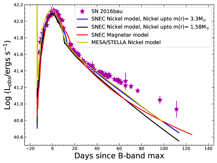
Figure 3.26: Comparison of the quasi-bolometric light curve of SN 2016bau and light curves produced by SNEC and STELLA, considering the radioactive decay model.

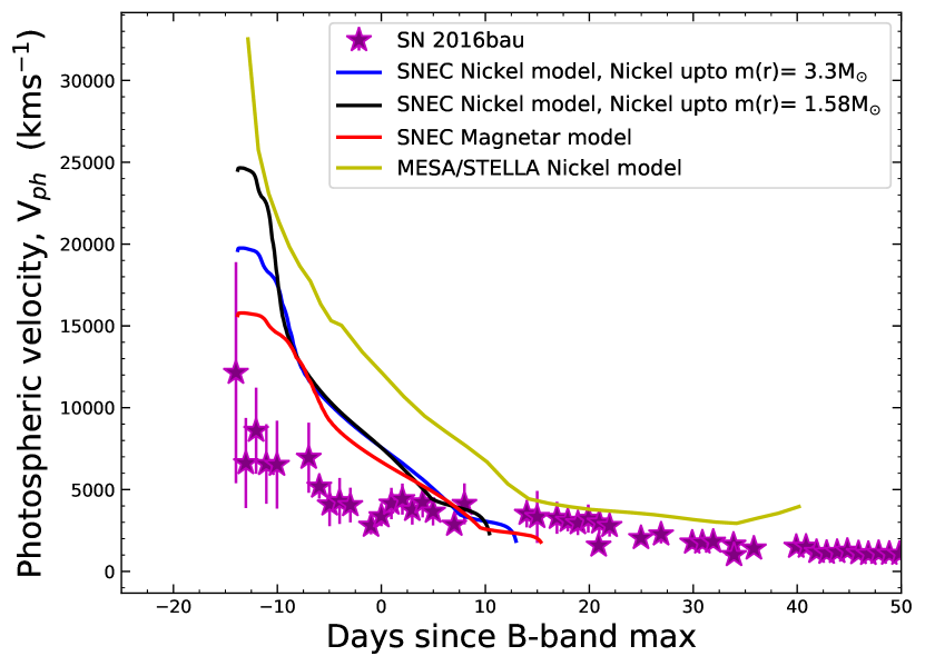
Figure 3.27: Comparison between the observed velocity evolution of SN 2016bau and the photometric velocity evolution produced by SNEC and STELLA, considering the radioactive decay model.

$\bullet$ Spin-down of a magnetar

We also tried the magnetar powering mechanism for SN 2016bau. The explosion is simulated as a piston, with the first two computational cells of the profile boosted outward with a velocity of 3.6$\times$10⁹ cm s^-1 for a duration of 0.01 s and a total model energy of 0.8$\times$10⁵¹ erg. Like SN 2015ap, we inject $L_{\mathrm{sd_{i}}}$ = 0.4$\times$10⁴³ erg s^-1 to the ejecta above the mass cut uniformly in mass. We assume $t_{\mathrm{sd}}$ = 16.0 d and do not include the effect of Ni heating. Corresponding to $L_{\mathrm{sd{{}_{i}}}}$ = 0.4$\times$10⁴³ erg s^-1 and $t_{\mathrm{sd}}$ = 16 d, we obtain a magnetic field ($B$) of 7.9$\times$10¹⁴ G and an initial period ($P_{i}$) of 71.8 ms for the modelled magnetar. These values of $B$ and $P_{i}$ are very close to those obtained using MINIM.

We also perform STELLA calculations for SN 2016bau by employing the default radioactive decay of ⁵⁶Ni and ⁵⁶Co powering mechanism. We used similar parameters as in the case of SNEC and STELLA. The MESA setups are unchanged for STELLA calculations. We used a total energy after explosion of 1.6$\times$10⁵¹ erg and a ⁵⁶Ni mass of 0.065 M_⊙, slightly above the ⁵⁶Ni mass used in SNEC.

$\bullet$ Summary of the modelling

Figure 3.26 shows the comparison of the observed quasi-bolometric luminosity with that produced by SNEC for the radioactive decay and magnetar spin-down models. We find that the radioactive decay model from SNEC could successfully explain the light curve. The magnetar model also shows a good match, but we do not see any significant signs of SN 2016bau being powered by a magnetar. This figure also shows the results of STELLA calculations; they also match the observed light curve of SN 2016bau nicely, with parameters similar to those of SNEC.

Figure 3.27 shows a comparison of the observed photospheric velocity evolution produced by blackbody fitting with that produced by the radioactive decay model and the magnetar spin-down model using SNEC. Here, the models show high initial velocities, which drop at later epochs. We see that the velocities produced by the models initially deviate from the observed photospheric velocities but tend to follow velocities similar to the observed ones at later epochs. The figure also shows a comparison of the Fe II 5169 Åline velocity obtained using STELLA with the photospheric velocity obtained through blackbody fits. Similar to the case of SN 2015ap, this SN also lacks unambiguous features of the Fe II 5169 Åline.

From Figure 3.27, it is evident that our model overestimates the velocity by a factor of nearly two. The $M_{\rm ej}$ from Arnett’s model is $\sim$ 1.6 M_⊙. The diffusion time is given by $(M^{3}/E)^{1/4}$. Since this combination is fixed, $M^{3}/E$ is roughly constant. But $M^{3}/E\approx M^{3}/(Mv^{2})=M^{2}/v^{2}\approx$ constant. Thus, we have $M\approx v$ to meet the observational constraints. So, if we need to decrease the velocity by a factor of two, the ejecta mass would also decrease by the same factor. Then the He star mass is likely $\sim$ 2–2.5 M_⊙, which is at the boundary between an SN and a non-SN. Since $E\approx Mv^{2}\approx v^{3}$, the energy may go down quite substantially in this case.

3.9 Discussion

We present a detailed photometric and spectroscopic analysis of two Type Ib SNe, namely SN 2015ap and SN 2016bau. From our analysis, SN 2015ap is an intermediate-luminosity normal SN Ib, while SN 2016bau is highly extinguished by host-galaxy dust. In this section, we discuss the major outcomes of our present analysis.

The photometric properties of both the SNe were analysed by determining the bolometric luminosity of their light curves. For SN 2015ap, we calculate a ⁵⁶Ni mass of 0.14$\pm$0.02 M_⊙ and an ejecta mass of 2.2$\pm$0.6 M_⊙, while for SN 2016bau, the ⁵⁶Ni mass and ejecta mass were 0.055$\pm$0.006 M_⊙ and 1.6$\pm$0.3 M_⊙, respectively. The photospheric temperature, radius, and velocity evolution for both SNe were also explored. Based on the derived physical quantities from the temporal evolution of these two SNe, we tried to constrain possible powering mechanisms using a semi-analytical model called MINIM. We found that the semi-analytical RD model failed to simultaneously fit both SNe’s early and late phases, raising issues related to the validity of such models in the case of stripped-envelope SNe. One solution to such a situation is to fit the early-phase and late-phase data with different sets of model parameters. Another cause for the failure of the RD model can be attributed to the assumption of the constant ejecta density profile. For the MAG model, the fitted parameters seemed to be unphysical in both SNe, especially the very slow initial rotation (for SN 2015ap, $P_{i}\approx$ 40 ms, and for SN 2016bau, $P_{i}\approx$ 70 ms) and the very low initial rotational energy (for both SNe, $E_{p}\approx$10⁴⁹ erg). Also, no signs of these SNe powered by a magnetar mechanism were evident either from photometry or spectroscopy, so this possibility was discarded.

The spectroscopic behaviour of both SNe was also studied using the present and archival data. These SNe showed unambiguous He I features from very early to late phases, confirming them to be SNe Ib. Their spectral features match those of other well-studied SNe Ib. Additionally, SN 2015ap closely resembled SN 2008D, which had shown X-ray emission. The spectra of our two SNe at various epochs were modelled using SYN++. For SN 2015ap, the spectral modelling indicated a range of photospheric temperatures and velocities from 13,000 km s^-1 to 6800 km s^-1 and from 12,000 K to 4500 K (respectively) during the time interval -7 d to +33 d. For SN 2016bau, these two parameters ranged from 16,000 km s^-1 to 8000 km s^-1 and from 9000 K to 4000 K (respectively) during the time interval -14 d to +33 d. The spectra of these two SNe at particular epochs were compared with model spectra of 12, 13, and 17 M_⊙ progenitor stars. For SN 2015ap, the 12 M_⊙ and 17 M_⊙ model spectra showed reasonable matches, indicating a progenitor in the mass range 12–17 M_⊙; for SN 2016bau, the 12 M_⊙ model spectrum could explain the observed spectrum to some extent better than other models, indicating a $\leq$ 12 M_⊙ progenitor.

Based on the photometric and spectroscopic properties described above, a 12 M_⊙ ZAMS star was chosen as the possible progenitor for both SNe. This 12 M_⊙ ZAMS progenitor was evolved up to the onset of core collapse using MESA. The MESA outputs on the onset of core collapse were fed as input to SNEC and STELLA, which simulate the synthetic explosions. The RD and MAG models were employed using SNEC while only the RD model was employed in STELLA. Here also, the models failed to fit the late part of the light curve simultaneously. The cause can be attributed to the various assumptions, including the spherically symmetrical explosions and the use of constant ejecta density profiles throughout. Similar to the case of MINIM, the MAG model provided unphysical parameters during the SNEC analysis.

Our analysis favours a 12 M_⊙ ZAMS star as a possible progenitor for SN 2015ap based on outputs of the models reasonably explaining the bolometric luminosity light curve and the photospheric velocity. However, in the case of SN 2016bau, the model velocities are higher by a factor of almost 2, demanding that the ejecta mass be lower by a similar factor. This would imply a helium star of mass $\sim$ 2–2.5 M_⊙, which is at the boundary for exploding as an SN. Thus, a slightly lower mass ZAMS star could also be the possible progenitor of SN 2016bau. Hydrodynamic evolution models of such low-mass stars to reach the stage of core collapse and then undergo synthetic explosions are extremely difficult to perform, but this can be taken as a challenge for the future.

3.10 Conclusions

Photometric and spectroscopic analyses of the Lick/KAIT-discovered Type Ib SN 2015ap and another Type Ib SN 2016bau, both having extensive follow-up observations made with various telescopes, are discussed. For both SNe, photometric data corrected for the Milky Way and host-galaxy extinction were used to estimate the quasi-bolometric luminosity light curves and study the photospheric radius, temperature, and velocity evolution. Spectral properties of SN 2015ap and SN 2016bau were then explored in detail. We modelled the spectra, studied the spectral evolution, and compared the spectra at various epochs with those of other well-studied SNe Ib, which further confirmed that these two SNe are Type Ib SN.

We attempted to determine the progenitor masses of SN 2015ap and SN 2016bau. Our results support 12 M_⊙ progenitors for these two SNe. The 12 M_⊙ ZAMS progenitor was evolved up to the onset of core-collapse using MESA. The output of MESA was incorporated as input to SNEC and STELLA, which produced the artificial explosions replicating the actual SN explosions. Considering the decay of Ni and Co to be the most prominent powering mechanism for SNe Ib, we tried this powering mechanism for SN 2015ap and SN 2016bau, using SNEC and STELLA. We found that the quasi-bolometric luminosity could nicely be explained by our models, while the velocity evolution obtained from SNEC and STELLA satisfactorily agrees with the observed one. We also explored the effect of the distribution of nickel mass near the centre and up to near the surface. Lower amounts of nickel were required to match the light curve for the case of centrally distributed nickel in comparison to the case where the nickel was distributed up to near the surface. Based on the above conclusions, our analysis supports a star having $M_{\rm ZAMS}$ = 12 M_⊙ as the possible progenitor for SN 2015ap. For SN 2016bau, a slightly lower ZAMS progenitor is expected.

Chapter 4 Low-luminosity Type IIb SN 2016iyc arising from a low mass progenitor

4.1 Introduction

After studying the temporal and spectral properties of two H-deficient Type Ib SNe followed by the stellar evolution and synthetic explosions of their possible progenitors in Chapter 3, we perform the photometric and spectroscopic analyses of a Type IIb SN in this Chapter. Type IIb SNe are a subclass of catastrophic CCSNe. These SNe form a transition class of objects that link H-rich Type II and H-deficient Type Ib SNe (Filippenko 1988; Matheson et al. 1993; Filippenko 1997; Smartt 2009). Their early-phase spectra show strong H features and distinct He-features start to appear a few weeks later; thus, these SNe are thought to be partially stripped by retaining some trace H-envelope, and the He core is exposed once the envelope becomes optically thin. It is relevant to mention that SNe Type Ib/IIb are differentiated just on the basis of the presence of some trace amount of hydrogen in the exploding star. However, the correct estimation of the retained amount of hydrogen is difficult due to the uncertainties associated with determining the extinction and distance of underlying CCSNe (Gilkis & Arcavi, 2022).

The predominant powering mechanisms in SNe IIb are the radioactive decay of ⁵⁶Ni and the deposition of internal energy by the shock in the ejecta (e.g., Arnett, 1980, 1982, 1996; Nadyozhin, 1994; Chatzopoulos et al., 2013; Nicholl et al., 2017). In a few cases, the SN progenitors are also surrounded by dense CSM; thus, the SN ejecta may violently interact with the CSM. The interaction of CSM with the SN ejecta results in the formation of a two-component shock structure: a forward shock moving into the CSM and a reverse shock moving back into the SN ejecta. Both of these shocks deposit their kinetic energies into the material that is radiatively released, powering the light curves of the SNe (e.g., Chevalier, 1982; Chevalier & Fransson, 1994; Moriya et al., 2011; Ginzburg & Balberg, 2012; Chatzopoulos et al., 2013; Nicholl et al., 2017).

Understanding the possible progenitors of stripped or partially-stripped CCSNe is a challenging task. Methods to investigate the SN progenitors and their properties include (a) direct detections of objects in pre-explosion images and (b) modelling of certain mass ZAMS stars as the possible progenitors based on the observed photometric and spectroscopic properties of the SNe. Direct detections of progenitors are rare owing to the uncertainty associated with the spatial positions and the infrequent occurrence of these transient phenomena. One has to be very lucky to get such pre-explosion images. However, for SNe IIb, four cases of the direct detection of objects in pre-explosion images have been claimed. These include SN 1993J (Richmond et al., 1993; Aldering et al., 1994), SN 2008ax (Crockett et al., 2008), SN 2011dh (Maund et al., 2011; Van Dyk et al., 2011), and SN 2013df (Van Dyk et al., 2014), indicating either massive Wolf-Rayet (WR) stars ($M_{\rm ZAMS}\approx 10$–28 M_⊙; Crockett et al. 2008) or more extended yellow supergiants (YSGs) with $M_{\rm ZAMS}$ = 12–17 M_⊙ (Van Dyk et al., 2013; Folatelli et al., 2014; Smartt, 2015) as SN IIb progenitors. Following Smartt et al. (2009) and Van Dyk (2017), there have only been $\sim 34$ cases of direct CCSNe progenitor detections. With these direct detections, the progenitors of SNe IIP are red supergiants (RSGs); SN IIn progenitors are luminous blue variables; the progenitors of SNe IIL are still debated, with only the case of SN 2009kr suggesting RSG or yellow supergiant progenitors; and the progenitors of SNe Ib/c are either low-mass stars in a binary system (Podsiadlowski et al., 1992; Nomoto et al., 1995; Smartt, 2009) or a single massive WR star (e.g., Gaskell et al., 1986; Eldridge et al., 2011; Groh et al., 2013).

The second method, progenitor modelling using stellar evolution codes to constrain the nature of the possible progenitors of stripped or partially-stripped CCSNe, identified either via direct imaging as in the case of iPTF13bvn (Cao et al., 2013) or indirect methods including nebular-phase spectral modelling (Jerkstrand et al., 2015; Uomoto, 1986), and simulating the synthetic explosions of their pre-SN models, is also vital to understand their nature, physical conditions, circumstellar environment, and chemical compositions. But, the progenitor modelling of such objects using various stellar evolution codes is difficult due to the complicated shell-burning stages. Another problem associated with such modelling is the obscure nature of the mixing-length-theory parameter ($\alpha_{\rm MLT}$). The basis of $\alpha_{\rm MLT}$ has no physical origin (Joyce & Chaboyer, 2018; Viani et al., 2018). Furthermore, Joyce & Chaboyer (2018) mentions that $\alpha_{\rm MLT}$ is neither a physical constant nor a computational one; it is rather a free parameter, so the value of $\alpha_{\rm MLT}$ must be determined individually in each stellar evolution code.

Owing to the above-mentioned difficulties, only a handful of such studies, including progenitor modelling followed by their synthetic explosions, have been performed in the case of stripped or partially-stripped CCSNe, including the Type Ib SN iPTF13bvn (Cao et al., 2013; Bersten et al., 2014; Paxton et al., 2018), the famous Type IIb SN 2016gkg (Bersten et al., 2018), a few other Type IIb SNe including SN 2011dh (Bersten et al., 2012), SN 2011fu (Morales-Garoffolo et al., 2015), two Type Ib SNe 2015ap and 2016bau (results presented in Chapter 3), and another Type Ib SN 2012au (Pandey et al., 2021).

Considering these limited studies, our work goes one step further, as we perform the 1-dimensional stellar evolution of the possible progenitor models for the low-luminosity Type IIb SN 2016iyc and simulate synthetic explosions. Our studies in this work point toward SN 2016iyc originating from the lower-mass end of the ZAMS progenitor systems observed for Type IIb CCSNe.

This Chapter is divided into eight sections, including an introduction in Sec. 4.1. Sec. 4.2 provides details about various telescopes and reduction procedures, including the discovery of SN 2016iyc using the KAIT at Lick Observatory as well as recalibrated photometry of SN 2016gkg. In Sec. 4.3, methods to correct for the extinction, photometric properties, including the bolometric light curve, blackbody temperature, and radius evolutions, are discussed. We present the analyses describing the spectral properties and comparisons with other similar and well-studied SNe in Sec. 4.4; we also model the spectra of these SNe using SYN++. The assumptions and methods for modelling the possible progenitor of SN 2016iyc and the evolution of the models until the onset of core collapse using MESA are presented in Sec. 4.5. Further, in this section, we discuss the assumptions and methods for simulating the synthetic explosions using SNEC and STELLA. Here, comparisons between the parameters obtained through synthetic explosions and observations are presented. We also perform hydrodynamic modelling of the synthetic explosions of SN 2016gkg and SN 2011fu in Sec. 4.6. In Sec. 4.7, we discuss our major results and findings. We summarise our work and provide concluding remarks in Sec. 4.8.

4.2 Data acquisition and reduction

SN 2016iyc was discovered by Kouchkovsky et al. (2016) in an 18 s unfiltered image taken at 03:28:00 on 2016 Dec. 18 (UT dates are used throughout this Chapter) by the 0.76 m KAIT as part of the Lick Observatory Supernova Search (LOSS). Its brightness was $17.81\pm 0.11$ mag, and the object was not detected earlier on Dec. 04.14 with an upper limit of 19.0 mag. We measure its J2000.0 coordinates to be $\alpha=22^{\rm h}09^{\rm m}14.^{\rm s}29$, $\delta=+21^{\circ}31^{{}^{\prime}}17.^{{}^{\prime\prime}}3$, with an uncertainty of $0.^{{}^{\prime\prime}}5$ in each coordinate. SN 2016iyc is $14.^{{}^{\prime\prime}}0$ west and $10.^{{}^{\prime\prime}}4$ north of the nucleus of the host galaxy UGC 11924, which has redshift $z$ = 0.012685$\pm$0.000017 (Giovanelli & Haynes, 1993), with a spiral morphology (Sd).

$B$, $V$, $R$, and $I$ multiband follow-up images of SN 2016iyc were obtained with both KAIT and the 1 m Nickel telescope at Lick Observatory; KAIT also obtained additional unfiltered (Clear (C)-band) images. Although unfiltered and thus nonstandard, $C$ is most similar to the $R$ band (Li et al., 2003), and has been widely used for SN observations by KAIT.

All images were reduced using a custom pipeline detailed by Stahl et al. (2019). Here we briefly summarise the photometric procedure. Image subtraction was conducted to remove the host-galaxy contribution, using additional images obtained after the SN had faded below the detection limit. Point-spread-function (PSF) photometry was obtained using DAOPHOT (Stetson, 1987) from the IDL Astronomy User’s Library. Several nearby stars were chosen from the Pan-STARRS1 catalogue for calibration purpose; their magnitudes were first transformed into the Landolt (1992) system using the empirical prescription presented by Tonry et al. (2012, Eq. 6), and then into the KAIT/Nickel natural system. All apparent magnitudes were measured in the KAIT4/Nickel2 natural system. The final results were transformed to the standard system using local calibrators and colour terms for KAIT4 and Nickel2 (Stahl et al., 2019).

The same method was adopted to reprocess the LOSS data of SN 2016gkg (originally published by Bersten et al. 2018), except that no subtraction procedure was applied to SN 2016gkg; the calibration source was also chosen from the Pan-STARRS1 catalogue. Photometry of SN 2016gkg at two epochs was also obtained with the 3.6 m Devasthal optical telescope (DOT) using the 4K$\times$4K CCD Imager. SN 2016gkg was the first SN detected by the 3.6 m DOT during its initial commissioning phases. For the data obtained from the 3.6 m DOT, the Landolt (1992) photometric standard fields PG 0918, PG 1633, and PG 1657 were observed on 2021 Feb. 07 along with the SN field in the $UBVRI$ bands under good photometric conditions. These three Landolt fields have standard stars with a $V$-band magnitude range of 12.27–15.26 mag and a $B-V$ colour range of $-$0.27 to +1.13 mag. The SN fields observed in 2021 were used for template subtraction to remove the host-galaxy contributions from the source images. Template subtraction was performed with standard procedures by matching the full width at half-maximum intensity (FWHM) and flux values of respective images. The optical photometric data reduction and calibration were made with a standard process discussed by Kumar et al. (2021) and Python scripts hosted on RedPipe (Singh, 2021). The average atmospheric extinction values in the $U$, $B$, $V$, $R$, and $I$ bands for the Devasthal site were adopted from Kumar et al. (2022b). The recalibrated KAIT data of SN 2016gkg, along with those observed at later epochs using the 4K$\times$4K CCD Imager mounted at the axial port of the 3.6 m DOT were utilised for the construction of bolometric light curves as described in the following sections.

A single optical spectrum of SN 2016iyc was obtained on 2016 Dec. 23 with the Kast double spectrograph mounted on the 3 m Shane telescope at Lick Observatory. The 2700 s exposure was taken at or near the parallactic angle to minimise slit losses caused by atmospheric dispersion (Filippenko, 1982). The observations were conducted with a $2^{\prime\prime}$-wide slit, 600/4310 grism on the blue side, and 300/7500 grating on the red side. This instrument configuration has a combined wavelength range of $\sim 3500$–10,400 Åand spectral resolving power of $R\approx 800$. Data reduction followed standard techniques for CCD processing and spectrum extraction (Silverman et al., 2012) utilising IRAF routines and custom Python and IDL codes. Low-order polynomial fits to comparison-lamp spectra were used to calibrate the wavelength scale, and small adjustments derived from night-sky lines in the target frames were applied. Observations of appropriate spectrophotometric standard stars were used to flux calibrate the spectrum.

4.3 Photometric Properties

In this section, we discuss the photometric properties of SN 2016iyc, including colour evolution, extinction, bolometric light curves, and various blackbody parameters. Most of the analyses in this Chapter have been performed with respect to the phase of $V$-band maximum brightness. The photometric data of SN 2016iyc lack dense coverage near peak brightness; thus, to find the phase of $V$-band maximum, we used the $V$-band light curve of SN 2013df as a template having a rising timescale similar to that of SN 2016iyc (Figure B.1). We fit a fourth-order polynomial to the template light curve and find the date of $V$ maximum to be MJD $57752.7\pm 0.2$. The left panel of Figure 4.1 shows the $BVRI$- and $C$-band light curves of SN 2016iyc. The characteristic extended shock-breakout (hereafter, extended-SBO) feature typically observed in SNe IIb is seen in all of the bands. Multiple mechanisms and/or ejecta/progenitor properties have been theorised to explain such enhancement in the luminosity before the primary peak, including an increase in the progenitor radius up to a few 100 R_⊙ (e.g. Nomoto et al., 1993; Podsiadlowski et al., 1993; Woosley et al., 1994); an interaction with CSM similar to the case of Type IIn SNe (Schlegel, 1990); in a close-binary system, the interaction with the companion (Kasen & Bildsten, 2010; Moriya et al., 2015); and sometimes enhanced ⁵⁶Ni mixing into the outer ejecta (e.g., Arnett & Fu, 1989). The right-hand panel of Figure 4.1 shows the $BVRI$ and $C$ light curves along with the late-time upper limits in each band. These upper limits are very useful in constraining the upper limit on $M_{\rm Ni}$.

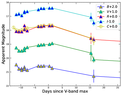
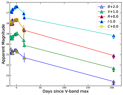
Figure 4.1: Left: The $BVRI$- and $C$-band light curves of SN 2016iyc, obtained with KAIT. The generic extended-SBO feature of SNe IIb is visible in each band. Right: The $BVRI$ and $C$ light curves along with the upper limits in each band using the Las Cumbres Observatory global telescope network. The upper limits in the last epoch are extremely useful for setting an upper limit on $M_{\rm Ni}$.

4.3.1 Distance estimation of SN 2016iyc

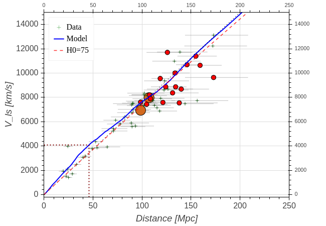
Figure 4.2: Distance estimation for the nearby ($z$ = 0.012685) SN 2016iyc using the method described by Kourkchi et al. (2020) with Graziani et al. (2019) models. The distance value estimated with this method is $\sim 10$ Mpc ($\sim 20$%) nearer than that reported using the published redshift value (Planck Collaboration et al., 2016) for SN 2016iyc.

Distance determinations from redshifts ($z$) are severely biased for nearby SNe because of the peculiar motions of nearby galaxies that are comparable to the Hubble flow. So, the redshift-based distance estimates can be used only for SNe having $z$ $>$ 0.1. Hence, the redshift-based distance for SN 2016iyc, published by Planck Collaboration et al. (2016), could be spurious. SN 2016iyc being nearby ($z$ = 0.012685), we cross-verified the redshift-based distance estimate (56.6837 Mpc as mentioned by Planck Collaboration et al. 2016) with an advanced tool (Figure 4.2) recently featured by Kourkchi et al. (2020), known as the Distance-Velocity ($D$–$V$) Calculator. Corresponding to a heliocentric velocity $V_{\rm h}\approx 3804$ km s^-1, the observed velocity ($V_{\rm ls}$) at the location of SN 2016iyc is found to be $\sim 4089$ km s^-1 by utilising Eq. 5 of Kourkchi et al. (2020). Corresponding to $V_{\rm ls}=4089$ km s^-1, the $D$–$V$ Calculator gives a distance of $\sim 46$ Mpc, which is $\sim 20$% less than Planck Collaboration et al. (2016). The distance modulus for SN 2016iyc corresponding to this distance is 33.31 mag and is adopted for all further analyses in this Chapter. The distances for the SNe used as a comparison sample are well established in the literature and are used as such for the estimation of their respective bolometric luminosities. The distance of each SN in the comparison sample, along with the corresponding distance modulus is presented in Table 4.1.

Table 4.1: The adopted total extinction values, distances, and corresponding distance moduli of a subset of SNe considered here.

SN name	$E(B-V)_{\rm tot}$	Adopted distance	Distance modulus	$V_{\rm max}$	log $(L_{BVRI})_{p}$
	(mag)	(Mpc)	(mag)	(mag)	(erg s-1)
SN 1987A	0.16 (Bose et al., 2021)	0.05 (Bose et al., 2021)	18.44	$-15.52\pm 0.02$	42.555 $\pm$ 0.004
SN 1993J	0.18 (Richmond et al., 1996)	3.68 (Bose et al., 2021)	27.82	$-16.97\pm 0.03$	42.01 $\pm$ 0.01
SN 2003bg	0.02 (Mazzali et al., 2009)	24 (Mazzali et al., 2009)	31.90	-17.8$\pm$0.2	42.31 $\pm$ 0.03
SN 2008ax	0.3 (Tsvetkov et al., 2009)	9.6 (Pastorello et al., 2008)	29.92	$-16.35\pm 0.05$	42.07 $\pm$ 0.03
SN 2011dh	0.035 (Sahu et al., 2013)	8.4 (Sahu et al., 2013)	29.62	$-17.06\pm 0.02$	41.99 $\pm$ 0.03
SN 2011fu	0.22 (Kumar et al., 2013)	77.0 (Kumar et al., 2013)	34.46	$-17.51\pm 0.03$	42.426 $\pm$ 0.006
SN 2011hs	0.17 (Bufano et al., 2014)	23.44∗	31.85	$-16.03\pm 0.03$	41.74 $\pm$ 0.02
SN 2013df	0.098 (Morales-Garoffolo et al., 2015)	16.6 (Van Dyk et al., 2014)	31.1	$-16.47\pm 0.05$	41.87 $\pm$ 0.01
SN 2016gkg	0.017 (Bersten et al., 2018)	26.4 (Kilpatrick et al., 2017)	32.11	$-17.03\pm 0.05$	41.98 $\pm$ 0.02
SN 2016iyc	0.137	46.0	33.31	$-15.32\pm 0.05$	41.44 $\pm$ 0.01

The sources for the $BVRI$ light curves for SNe in the comparison sample are as follows. SN 1987A, Menzies et al. (1987) and Makino et al. (1987); SN 1993J, Zhang et al. (2004); SN 2003bg, Hamuy et al. (2009); SN 2008ax, Pastorello et al. (2008); SN 2011dh, Sahu et al. (2013); SN 2011fu, Kumar et al. (2013); SN 2011hs, Bufano et al. (2014); SN 2013df, Morales-Garoffolo et al. (2015). Adopted distances have been used to calculate the distance moduli. The total extinction correction and distance moduli for all the SNe in the comparison sample have been considered while calculating the bolometric light curves. ^∗For SN 2011hs, the distance modulus is 31.85 mag (Bufano et al., 2014), which is used to back-calculate a distance of 23.44 Mpc.

4.3.2 Colour evolution and extinction correction

For SN 2016iyc, we corrected for the Milky Way (MW) extinction using NED, following Schlafly & Finkbeiner (2011). In the direction of SN 2016iyc, $E(B-V)_{\rm MW}=0.067$ mag, so the MW extinction corrections for the $B$, $V$, $R$, and $I$ bands are 0.278, 0.207, 0.155, and 0.099 mag, respectively.

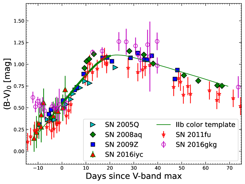
Figure 4.3: The total-extinction-corrected $(B-V)_{0}$ colour curves of SN 2016iyc, SN 2011fu, and SN 2016gkg, plotted along with other SNe IIb. The data for SN 2005Q, SN 2008aq, and SN 2009Z were taken from Stritzinger et al. (2018), with these three SNe analysed to have negligible host-galaxy extinction. The green curve shows the template $(B-V)_{0}$ curve for SNe IIb having negligible host-galaxy extinction. The thick portion of the template curve shows the 0 to +20 d period that should be considered when determining the colour excess for the reasons mentioned by Stritzinger et al. (2018).

Only one spectrum of SN 2016iyc is available, and it does not exhibit a clear Na I D absorption line produced by gas in the host galaxy, suggesting that there is negligible host-galaxy extinction. However, neglecting host-galaxy extinction based on only the absence of obvious Na I D could be spurious. In a Lick/KAIT data-release paper for various stripped-envelope SNe, Zheng et al. (2022) performed a comprehensive analysis to determine the host-galaxy contamination and found $E(B-V)_{\rm host}=0.07$ mag for SN 2016iyc. We also performed a simple analysis to put an upper limit on the host-galaxy extinction. Five early epochs were selected, and the spectral energy distribution (SED) was fitted with blackbody curves by assuming different $E(B-V)_{\rm host}$ values (Figure B.2). We found that going beyond 0.07 mag of host-galaxy extinction results in blackbody temperature exceeding 11,200 K. Such high temperatures are generally not seen in SNe IIb. Following Ben-Ami et al. (2015), the early-time blackbody temperatures associated with SN 1993J, SN 2011dh, and SN 2013df are 8200 K, 8200 K, and 7470 K, respectively. There have been only a few cases where the early blackbody temperature exceeds 11,000 K; one such example is SN 2001ig Ben-Ami et al. (2015), but this SN may have come from a compact WR binary progenitor system(Ryder et al., 2004).

Based on the above analyses and the results of Zheng et al. (2022), we adopt a host-galaxy extinction of 0.07 mag throughout this Chapter. Thus, a total (Milky Way + host-galaxy) extinction of $E(B-V)_{\rm tot}=0.137$ mag is adopted for SN 2016iyc. Figure 4.3 shows the comparison of total extinction corrected $(B-V)_{0}$ colour of SN 2016iyc with other similar SNe.

4.3.3 Bolometric light curves

Before computing the bolometric light curves, the absolute $V$-band light curve of SN 2016iyc is compared with a few other similar SNe IIb. The left panel of Figure 4.4 shows that SN 2016iyc lies toward the fainter end of the distribution.

Furthermore, to obtain the quasi-bolometric light curve, we make use of the SUPERBOL code (Nicholl, 2018). The extinction-corrected $B$, $V$, $R$, and $I$ data are provided as input to SUPERBOL. The light curve in each filter is then mapped to a common set of times through the processes of interpolation and extrapolation. Thereafter, SUPERBOL fits blackbody curves to the SED at each epoch, up to the observed wavelength range (4000–9000 Å), to give the quasi-bolometric light curve by performing trapezoidal integration.

The right-hand panel of Figure 4.4 shows the comparison of the quasi-bolometric light curve of SN 2016iyc with other well-studied SNe IIb as listed in Table 4.1. The peak quasi-bolometric luminosity (log $(L_{BVRI})_{p}$) of each SN has also been calculated by fitting a third-order polynomial to the quasi-bolometric light curve. As indicated by the right-hand panel of Figure 4.4, SN 2016iyc lies toward the fainter limit of SNe IIb in the comparison sample. It is also worth mentioning that the low-luminosity SNe with low ⁵⁶Ni yields are thought to arise from progenitors having masses near the threshold mass for producing a CCSN (Smartt et al., 2009).

Furthermore, the bolometric luminosity light curve of SN 2016iyc is also produced after considering the additional blackbody corrections to the observed $BVRI$ quasi-bolometric light curve by fitting a single black body to observed fluxes at a particular epoch and integrating the fluxes trapezoidally for a wavelength range of 100–25,000 Å using SUPERBOL. Figure B.3 shows the blackbody fits to the SED of SN 2016iyc. The top panel of Figure 4.5 shows the resulting quasi-bolometric and bolometric light curves of SN 2016iyc.

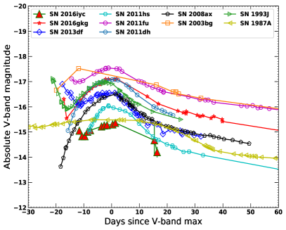
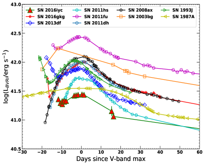
Figure 4.4: Left: Comparison of the absolute $V$-band light curves of SN 2016iyc and SN 2016gkg with other well-studied SNe IIb ( the peculiar Type II SN 1987A, included in the sample because of its low luminosity). Right: Comparison of the quasi-bolometric light curves of SN 2016iyc and SN 2016gkg with other well-studied SNe IIb obtained by integrating the fluxes over the $BVRI$ bands. SN 2016iyc lies toward the faint end of SNe IIb. The total extinction correction and distance moduli for all the SNe in the comparison sample have been taken into account while calculating these light curves.

Figure 4.5: The top panel shows the bolometric and quasi-bolometric light curves of SN 2016iyc. The luminosity corresponding to the late upper limits on $BVRI$ is shown later. The second and third panels from the top display the blackbody temperature and radius evolutions of SN 2016iyc, respectively.

4.3.4 Temperature and radius evolution

From SUPERBOL, the blackbody temperature ($T_{\rm BB}$) and radius ($R_{\rm BB}$) evolution of SN 2016iyc are also obtained. During the initial phases, the photospheric temperature is high, reaching $\sim 10,900$ K at $-10.63$ d. Furthermore, the SN seems to evolve very rapidly; its temperature quickly drops to $\sim 7600$ K in only a few days around $-7.7$ d and then remains nearly constant (Figure 4.5, second panel from top). Along with SN 2016iyc, the temperature evolutions of a few more similar SNe IIb are also shown in this panel. The blackbody temperature of SN 2016iyc seems to follow the typical temperature evolution as seen in SNe IIb.

A conventional evolution in radius is also seen. Initially, at an epoch of $-10.63$ d, the blackbody radius is $2.64\times 10^{14}$ cm. Thereafter, the SN expands and its radius increases, reaching a maximum radius of $\sim$ $5.8\times 10^{14}$ cm, beyond which the photosphere seems to recede into the SN ejecta (Figure 4.5, third panel from top). Along with SN 2016iyc, the blackbody radius evolutions of a few more similar SNe IIb are also shown. SN 2016iyc seems to exhibit anomalous behaviour, with its blackbody radii at various epochs being the smallest among other similar SNe IIb. This result can be attributed to the low ejecta velocity of SN 2016iyc.

4.4 Spectral Studies of SN 2016iyc

In this section, we identify the signatures of various lines by modelling the only available spectrum of SN 2016iyc using SYN++ (Branch et al., 2007; Thomas et al., 2011). We discuss various spectral features of SN 2016iyc, and the spectrum is also compared with other similar SNe.

4.4.1 Spectral modelling

A single optical spectrum of SN 2016iyc was obtained on 2016 Dec. 23 with the Kast double spectrograph (Miller & Stone, 1993) mounted on the 3 m Shane telescope at Lick Observatory. Figure 4.6 shows the spectral modelling of it, corresponding to a phase of $-6.6$ d. The individual lines corresponding to various elements and ions are also indicated for better identification of the features. The profiles of H$\alpha$ near 6563 Å, He I near 5876 Å, and Ca II H&K are very nicely reproduced by SYN++ modelling. A very strong H$\alpha$ feature near 6563 Å classifies SN 2016iyc as an SN IIb. The observed velocities obtained using H$\alpha$, He I, and Fe II features in the spectrum are $\sim 10,000$ km s^-1, $\sim 6700$ km s^-1, and $\sim 6100$ km s^-1 (respectively), while the respective velocities of these lines from SYN++ modelling are 10,100 km s^-1, 6800 km s^-1, and 6100 km s^-1, very close to the observed ones. The parameterisation velocity and photospheric velocity used to produce the SYN++ model are 6000 km s^-1 and 6100 km s^-1, respectively. Also, a photospheric temperature of 6300 K is employed to produce the model spectrum.

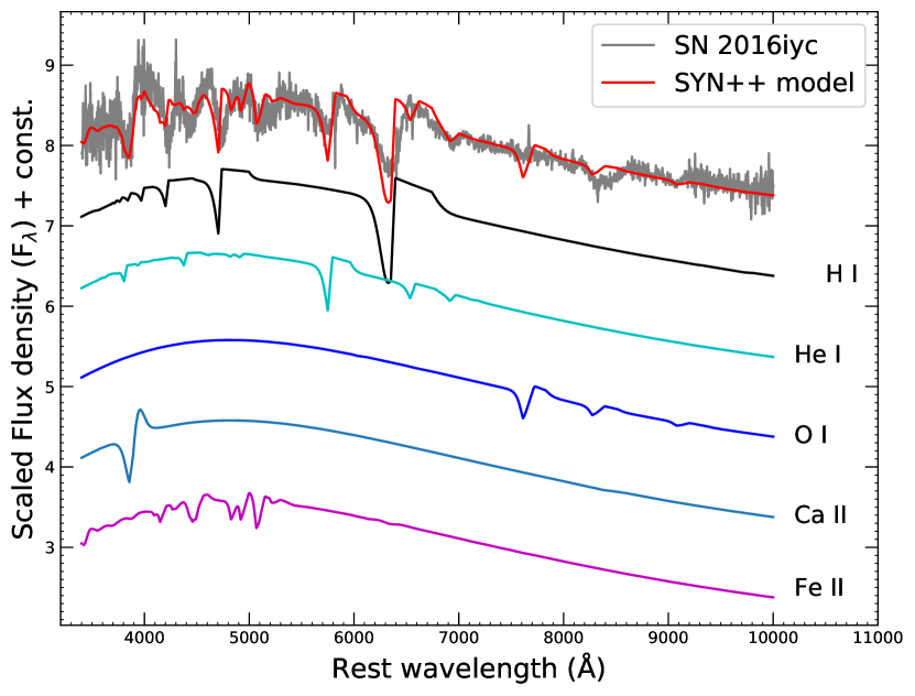
Figure 4.6: SYN++ modelling of the spectrum of SN 2016iyc at a phase of $-6.6$ d. The effects of various elements present in the SN ejecta and contributing to the spectrum are also displayed individually.

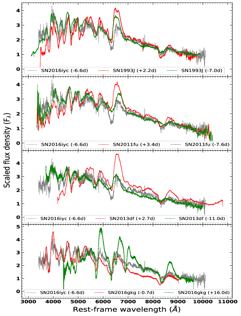
Figure 4.7: Comparison of the $-6.6$ d spectrum of SN 2016iyc with spectra of other well-studied SNe IIb, including SN 1993J, SN 2011fu, SN 2013df, and SN 2016gkg.

4.4.2 Spectral comparison

Figure 4.7 shows a comparison of the normalised spectrum of SN 2016iyc with other well-studied SNe IIb. The top plot displays the comparison with the spectra of SN 1993J at +2.3 d and $-7.0$ d; we see that the spectral features of SN 2016iyc closely resemble those of SN 1993J spectra. In the second panel from the top, the spectrum of SN 2016iyc is compared with the spectra of SN 2011fu at +3.4 d and $-7.0$ d; the match is close, except for the H$\alpha$ feature where the spectra of SN 2011fu are slightly off. The third panel from the top shows the spectral comparison of SN 2016iyc with spectra of SN 2013df at epochs of +2.7 d and $-11.0$ d, revealing a good match with the $-11.0$ d spectrum. The progenitor of SN 2013df is also thought to be arising from the lower-mass end. In the bottom panel, the spectrum of SN 2016iyc is compared with the spectra of SN 2016gkg at epochs of $-0.7$ d and +16 d. The $-0.7$ d spectrum of SN 2016gkg resembles the spectrum of SN 2016iyc toward the bluer side, while features in the redder part of the spectrum are slightly off. The +16 d spectrum of SN 2016gkg does not show a good resemblance with the spectrum of SN 2016iyc. From Figure 4.7, we conclude that the spectrum of SN 2016iyc shows a close resemblance with the spectra of other well-studied SNe IIb, thereby providing good evidence for the classification of SN 2016iyc as an SN IIb.

4.5 Possible Progenitor Modelling and the Results of Synthetic Explosions for SN 2016iyc

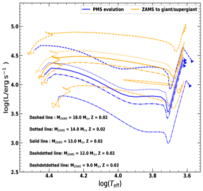
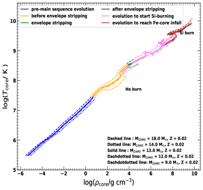
Figure 4.8: Left: The evolution of 9.0 M_⊙, 12 M_⊙, 13 M_⊙, 14 M_⊙, and 18.0 M_⊙ ZAMS progenitors with Z = 0.02 on the HR diagram. The models begin evolution on the pre-main sequence (blue curve), then reach the main sequence and evolve until they become giants/supergiants with being ready to strip their outer envelopes (orange curve). Right: The variation of core-temperature with a core-density as the models evolve through various phases on the HR diagram. The core-He and core-Si burning phases are marked. The onset of Fe-core infall in the models is marked by the core temperatures and core densities reaching above $10^{10}$ K and $10^{10}$ g cm^-3, respectively.

To constrain the physical properties of the possible progenitor of SN 2016iyc, we attempted several progenitor models. Following the available literature, SN 2016iyc lies near the faint limit (see Table 4.1), with $M_{\rm ej}$ also close to the lowest limit (Table 4.2). As mentioned earlier, low-luminosity SNe with low ⁵⁶Ni production are thought to arise from progenitors having masses near the threshold mass for producing CCSNe (Smartt, 2009). With low $M_{\rm ej}$ among typical SNe IIb and having intrinsically low luminosity, we started with the nearly lowest possible ZAMS progenitor mass of 9 M_⊙ for a Type IIb SN. Starting from the pre-main sequence, the model could be evolved up to the onset of core collapse. But the 9 M_⊙ model at the pre-SN phase in our simulation is very compact, having a radius of only 0.14 R_⊙. Such a compact progenitor cannot generate the generic extended-SBO feature of typical SNe IIb. Furthermore, no direct observational signatures have been found for an SN IIb arising from a progenitor having ZAMS mass $\leq 11$ M_⊙, so we do not make any further attempt to model progenitors having masses $\leq 11$ M_⊙. Thus, we select models having ZAMS masses of 12, 13, and 14 M_⊙, and evolve them up to the onset of core collapse. Such models originating from the lower limits of progenitor mass systems lack sufficiently strong winds to suffer much stripping; thus, the models are artificially stripped to mimic the effect of a binary companion. A brief description of our models is provided below.

Table 4.2: Ejecta masses of various SNe IIb and SN 2016iyc.

SN name	$M_{\rm ej}$	source
SN 1993J	1.9–3.5	Young et al. (1995)
SN 2003bg	4	Mazzali et al. (2009)
SN 2008ax	2–5	Taubenberger et al. (2011)
SN 2011dh	1.8–2.5	Bersten et al. (2012)
SN 2011fu	3.5	Morales-Garoffolo et al. (2015)
SN 2011hs	1.8	Bufano et al. (2014)
SN 2013df	0.8–1.4	Morales-Garoffolo et al. (2014)
SN 2016gkg	3.4	Bersten et al. (2018)
SN 2016iyc	1.2	Zheng et al. (2022)

We first evolve the nonrotating 9, 12, 13, and 14 M_⊙ ZAMS stars until the onset of core collapse, using the 1-dimensional stellar evolution code MESA (Paxton et al., 2011, 2013, 2015, 2018).

For the 9 M_⊙ model, $\alpha_{\rm MLT}=2.0$ is used throughout the evolution, except for the phase when the model evolves to reach the beginning of core-Si burning (i.e., in the inlist_to_si_burn file), where $\alpha_{\rm MLT}=0.01$ is used. At this phase, the evolution of the models is extremely sensitive to this $\alpha_{\rm MLT}$, since even a slight change (say, 0.02) results in the failure of the beginning of core-Si burning. Although $\alpha_{\rm MLT}=0.01$ seems to be very low, this is required for the successful evolution of considered models through the last phases of their evolution. Furthermore, as mentioned by Joyce & Chaboyer (2018), $\alpha_{\rm MLT}$ is neither a physical constant nor a computational one; it is rather a free parameter, so its value must be determined on an individual basis in each stellar evolution code. Thus, as $\alpha_{\rm MLT}=0.01$ is helpful for evolving the models beyond the beginning of core-Si burning, it is acceptable. For the 12, 13, and 14 M_⊙ models, $\alpha_{\rm MLT}=3.0$ is used throughout the evolution.

Convection is modelled using the mixing theory of Henyey et al. (1965), adopting the Ledoux criterion. Semiconvection is modelled following Langer et al. (1985) with an efficiency parameter of $\alpha_{\mathrm{sc}}=0.01$. For the thermohaline mixing, we follow Kippenhahn et al. (1980), and set the efficiency parameter as $\alpha_{\mathrm{th}}=2.0$. We model the convective overshoot with the diffusive approach of Herwig (2000), with $f=0.001$ and $f_{0}=0.007$ for all the convective cores and shells. We use the “Dutch” scheme for the stellar wind, with a scaling factor of 1.0. The “Dutch” wind scheme in MESA combines results from several papers. Specifically, when $T_{\mathrm{eff}}>10^{4}$ K and the surface mass fraction of H is greater than 0.4, the results of Vink et al. (2001) are used, and when $T_{\mathrm{eff}}>10^{4}$ K and the surface mass fraction of H is less than 0.4, the results of Nugis & Lamers (2000) are used. In the case when $T_{\mathrm{eff}}<10^{4}$ K, the de Jager et al. (1988) wind scheme is used.

SNe IIb have been considered to originate from massive stars which have retained a significant amount of their H-envelope. We have adopted a mass-loss rate of $\dot{M}\gtrsim 10^{-4}$ M${}_{\odot}\,\mathrm{yr}^{-1}$ to artificially strip the models until the final $M_{\rm H}$ reaches in range of (0.013–0.055) M_⊙. Such extensive mass loss rates are supported by the studies performed by Ouchi & Maeda (2017), where they mention that the binary scenario for the progenitors of SNe IIb leads to such high mass-loss rates. Furthermore, van Loon et al. (2005) have also reported extensive mass-loss rates reaching $\dot{M}=10^{-4}$ M${}_{\odot}\,\mathrm{yr}^{-1}$, solely by a single stellar wind.

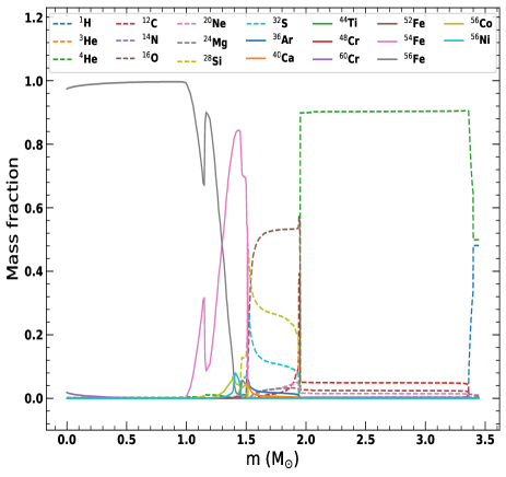
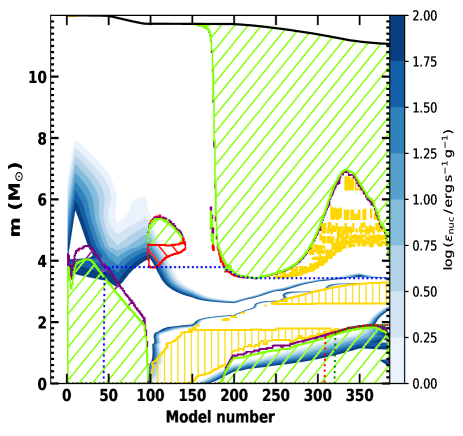
Figure 4.9: Left: The mass fractions of a few key elements when the 12 M_⊙ ZAMS progenitor model with Z = 0.02 has just reached the stage of Fe-core infall. Notice the very high mass fraction of ⁵⁶Fe in the core compared to other species. Right: The Kippenhahn diagram of the same model for a period from the beginning of main-sequence evolution to the stage when the model is ready to be stripped.

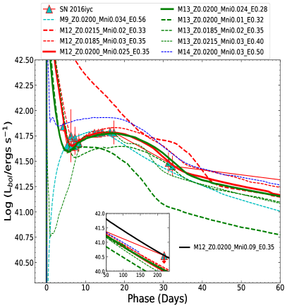
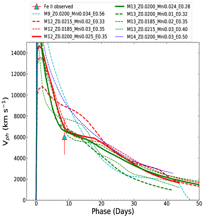
Figure 4.10: The results of the synthetic explosions produced using STELLA/SNEC by assuming 9 M_⊙, 12 M_⊙, 13 M_⊙, and 14 M_⊙ ZAMS stars as the possible progenitors for SN 2016iyc. Left: The bolometric luminosity light curves corresponding to different models having different metallicities, explosion energies, and nickel masses compared with the observed bolometric light curve of SN 2016iyc. Right: The corresponding photospheric velocity evolution comparison. In both the panels, the “Phase” is (approximate) days since the explosion. Following Zheng et al. (2022), the adopted phase of explosion is $-4.64^{+0.67}_{-0.76}$ since first detection that corresponds to MJD $57736.47^{+0.67}_{-0.76}$. The velocities produced by the models are well within the error bar of the observed photospheric velocities indicated by the Fe II line velocity.

Once the models have stripped off up to the specified limit of the H-envelope, we switch off the artificial mass loss and further evolve the models until the onset of core collapse. Corresponding to various ZAMS masses, the amount of remaining H varies. Massive progenitors with a similar rate of stripping as less-massive progenitors will retain a larger amount of H. In our simulations, the specified limit on H mass depends primarily on (a) the model’s ability to evolve up to the stage of core collapse by retaining the specified amount of H (also, there is a limit on stripping), and (b) the radius of the pre-SN progenitor. If we need a compact progenitor, the amount of retained H is less, and if pre-SN progenitors are required to have extended envelopes, the amount of retained H is more.

The evolution of the models using MESA takes place in various steps. The models start to evolve on the pre-main sequence and reach the main sequence. The arrival of the models on the main sequence is marked when the ratio of the luminosity due to nuclear reactions and the total luminosity of the models is 0.8. Later, the models further evolve on the main sequence, becoming giants or supergiants. As a next step, artificial stripping of the models is performed, after which they are allowed to settle down. Once the stripping of the models reaches the specified H-envelope mass limit and the models have settled down, they further evolve until the ignition of Si burning in their core. Once the Si burning has started in the core, the models begin to develop an inert iron core, which is responsible for their cores to collapse.

The evolution of such models having ZAMS masses of 9, 12, 13, and 14 M_⊙ with metallicity Z = 0.0200 on the Hertzsprung-Russell (HR) diagram is illustrated in the left panel of Figure 4.8. We simulated a total of 9 models covering progenitor masses of 9–14 M_⊙ and also covering subsolar to supersolar metallicity wherever necessary. The pre-explosion properties using MESA and explosion properties using STELLA/SNEC are listed in Table 4.3. The models have been so named that they include the pieces of information of ZAMS mass, metallicity, $M_{\rm Ni}$, and $E_{\rm exp}$. Thus, the model M9.0_Z0.0200_Mni0.034_E0.56 has a ZAMS mass of 9 M_⊙, Z = 0.0200, $M_{\rm Ni}=0.034$ M_⊙, and $E_{\rm exp}=0.56\times 10^{51}$ erg.

The right-hand panel of Figure 4.8 shows the variation of core temperature ($T_{\rm core}$) with core density ($\rho_{\rm core}$) as the models evolve through various phases on the HR diagram. The core-He and core-Si burning phases are marked. The onset of core collapse is marked by $T_{\rm core}$ and $\rho_{\rm core}$ reaching above $\sim 10^{10}$ K and $10^{10}$ g cm^-3, respectively. The left panel of Figure 4.9 shows the mass fractions of various species present when the 12 M_⊙ model (with Z = 0.0200) has achieved Fe-core infall. The core comprises ⁵⁶Fe with negligible fractions of other species. Significant fractions of heavier metals are seen toward the surface of the pre-explosion progenitor. The right-hand panel of Figure 4.9 shows the Kippenhahn diagram for the 12 M_⊙ model (with Z = 0.0200) for a period from the beginning of main-sequence evolution to the stage when the model is ready to begin envelope stripping. In this figure, the convective regions are marked by the hatchings with the logarithm of the specific nuclear energy generation rate ($\epsilon_{\rm nuc}$) inside the stellar interiors marked with blue colours. The dark-yellow regions indicate the stellar interior where the thermohaline mixing is going on.

Table 4.3: MESA model and STELLA/SNEC explosion parameters of various models for SN 2016iyc.

Model Name	$M_{\rm ZAMS}$	Z	$M_{\mathrm{H}}^{a}$	$R_{\mathrm{0}}^{b}$	$f_{ov}^{c}$	$M_{\mathrm{f}}^{d}$	$M_{\mathrm{ci}}^{e}$	$M_{\mathrm{cf}}^{f}$	$M_{\mathrm{ej}}^{g}$	$M_{\mathrm{Ni}}^{h}$	$E_{\mathrm{exp}}^{i}$
	(M⊙)		(M⊙)	(R⊙)		(M⊙)	(M⊙)	(M⊙)	(M⊙)	(M⊙)	($10^{51}$ erg)
M9.0_Z0.0200_Mni0.034_E0.56	9.0	0.0200	0.013	0.14	0.007	2.17	1.4	1.4	0.77	0.034	0.56
M12.0_Z0.0215_Mni0.02_E0.33	12.0	0.0215	0.035	596	0.007	3.96	1.54	1.54	2.42	0.02	0.33
M12.0_Z0.0185_Mni0.03_E0.35	12.0	0.0185	0.055	315	0.007	3.49	1.46	1.46	2.03	0.03	0.35
M12.0_Z0.0200_Mni0.025_E0.35	12.0	0.0200	0.05	300	0.007	3.45	1.52	1.52	1.93	0.025	0.35
M12.0_Z0.0200_Mni0.09_E0.35	12.0	0.0200	0.05	300	0.007	3.45	1.52	1.52	1.93	0.09	0.35
M13.0_Z0.0200_Mni0.024_E0.28	13.0	0.0200	0.04	204	0.007	3.79	1.64	1.90	1.88	0.024	0.28
M13.0_Z0.0200_Mni0.01_E0.32	13.0	0.0200	0.04	204	0.007	3.79	1.64	1.64	2.15	0.01	0.32
M13.0_Z0.0185_Mni0.02_E0.35	13.0	0.0185	0.06	318	0.007	3.92	1.53	1.56	2.36	0.02	0.35
M13.0_Z0.0215_Mni0.03_E0.40	13.0	0.0215	0.015	10	0.007	3.81	1.61	1.62	2.19	0.03	0.40
M14.0_Z0.0200_Mni0.03_E0.50	14.0	0.0200	0.03	55	0.007	4.23	1.54	1.54	2.69	0.03	0.50

^aAmount of hydrogen retained after stripping. ^bpre-SN progenitor radius. ^cOvershoot parameter. ^dFinal mass of pre-SN model. ^eInitial mass of the central remnant. ^fFinal mass of the central remnant. ^gEjecta mass. ^hNickel mass. ⁱExplosion energy.

Using the progenitor models on the verge of core-collapse obtained through MESA, we carried out radiation hydrodynamic calculations to simulate the synthetic explosions. For this purpose, we used STELLA(Blinnikov et al., 1998, 2000, 2006) and SNEC (Morozova et al., 2015). STELLA solves the radiative transfer equations in the intensity momentum approximation in each frequency bin, while SNEC is a 1-dimensional Lagrangian hydrodynamic code that solves the radiation energy transport equations in the flux-limited diffusion approximation. STELLA and SNEC, both generate the bolometric light curve and the photospheric velocity evolution of the SN, along with a few other observed parameters. The radioactive decay of ⁵⁶Ni to ⁵⁶Co is considered to be one of the prominent mechanisms for powering the primary peak of SNe IIb. Both of these codes incorporate this model by default. Thus in this section, we model the entire bolometric light curve of the SN 2016iyc assuming this powering mechanism. Here, we provide the setup of the explosions to incorporate the Ni–Co decay model. The setups for simulating the synthetic explosion using SNEC and STELLA closely follow Ouchi & Maeda (2019) and the settings used in Chapter 3, respectively. Here, we briefly summarise the important parameters and modifications.

We simulate the synthetic explosions of the 9 M_⊙ model using SNEC. First, the innermost 1.4 M_⊙ is excised before the explosion, assuming that the model collapses to form NSs. The number of grid cells is set to be 1000 so that the light curves and photospheric velocities of the SNe from synthetic explosions are well converged in the time domain of interest.

For the M9.0_Z0.0200_Mni0.034_E0.56 model, the synthetic explosion is carried out using SNEC. The explosion is simulated as a Thermal_Bomb by adding $0.56\times 10^{51}$ erg of energy in the inner 0.1 M_⊙ of the model for a duration of 0.1 s. SNEC does not include a nuclear-reaction network, so the amount of ⁵⁶Ni is set by hand. A total of 0.034 M_⊙ of ⁵⁶Ni is distributed from the inner boundary up to the mass coordinate $m(r)=2.0$ M_⊙.

For the models having ZAMS masses of 12, 13, and 14 M_⊙, we used STELLA to simulate the synthetic explosions. The pre-SN model masses from 12 M_⊙ models lie in the range of (3.45–3.96) M_⊙, while from 13 M_⊙ models, the pre-SN model masses lie in the range (3.79–3.81) M_⊙. Furthermore, the 14 M_⊙ model has a pre-SN mass of 4.23 M_⊙ and is thus prone to produce a much higher $M_{\rm ej}$ than required for SN 2016iyc. For producing the synthetic explosions, the hydrodynamic simulations are performed using Thermal_Bomb-type explosion. Various explosion parameters, including the ejecta masses, synthesised nickel masses, and explosion energies corresponding to different models, are presented in Table 4.3

The results of the hydrodynamic simulations are shown in Figure 4.10. The left panel of Figure 4.10 shows the comparison of the SNEC- and STELLA-calculated bolometric light curves with the observed bolometric light curve (see Sec. 4.3.3 for details on bolometric light curves) produced by fitting black bodies to the SEDs and integrating the fluxes over the wavelength range of 100–25,000 Å, while the right-hand panel shows the comparison of the corresponding photospheric velocities with the photospheric velocity obtained using the only available spectrum indicated by the Fe II line velocity. The M9 M_Z0.0200_Mni_0.034_E0.56 model could match the observed stretch factor and the peak of the bolometric light curve, but it fails to reproduce the early extended SBO feature. The failure in producing the generic extended-SBO feature could be associated to the compactness of the pre-SN model having a radius of only 0.14 R_⊙.

Moreover, all of the remaining models generate the generic extended-SBO feature. Still, only the M12.0_M_Z0.0200_Mni0.025_E0.35 could generate the extended-SBO and overall bolometric light curve that could match with the actual bolometric light curve of SN 2016iyc. Another model that could nearly match the SN 2016iyc bolometric light curve is M13.0_M_Z0.0200_Mni0.024_E0.28. The remaining models deviate largely from the observed bolometric light curve of SN 2016iyc (left panel, Figure 4.10). From the right-hand panel of Figure 4.10, we find that the photospheric velocity evolution generated by the models, M13.0_M_Z0.0200_Mni0.01_E0.25 and M12.0_M_Z0.0200_Mni0.025_E0.35 pass closely to the observed line velocity from Fe II which is a good indicator of observed photospheric velocity.

We also have an upper limit on the bolometric luminosity of SN 2016iyc at a phase nearly 220 d since the explosion. In order to match the upper limit of the luminosity at that epoch, the model M12.0_M_Z0.0200_Mni0.025_E0.35 requires $M_{\rm Ni}=0.09$ M_⊙ (please take a look at the inset plot in the left panel of Figure 4.10; M12.0_M_Z0.0200_Mni0.09_E0.35 is the corresponding model), serving as an upper limit on the synthesised nickel in SN 2016iyc.

Anderson (2019) has estimated a median value of 0.102 M_⊙ for the nickel mass by considering 27 SNe IIb. Moreover, Afsariardchi et al. (2021) have also estimated the Ni mass for eight SNe IIb and found that except for SN 1996cb ($M_{\rm Ni}=0.04\pm 0.01$ M_⊙) and SN 2016gkg ($M_{\rm Ni}=0.09\pm 0.02$ M_⊙), each SN IIb has higher $M_{\rm Ni}$ than 0.09 M_⊙. These comparisons show that SN 2016iyc definitely suffered low nickel production. Thus, the 1-dimensional stellar evolution of various models, along with the hydrodynamic simulations of their explosions, suggest that a ZAMS progenitor having mass in the range 12–13 M_⊙ with $M_{\rm ej}$ in the range (1.89–1.93) M_⊙, $M_{\rm Ni}<0.09$ M_⊙, and $E_{\rm exp}$ = (0.28–0.35) $\times 10^{51}$ erg could be the possible progenitor of SN 2016iyc.

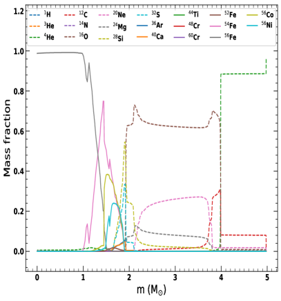
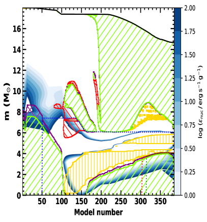
Figure 4.11: Left: The mass fractions of a few key elements when the 18 M_⊙ ZAMS progenitor model with Z = 0.02 has just reached the stage of Fe-core infall. The mass fraction of ⁵⁶Fe in the centre is much higher compared to other species. Right: The Kippenhahn diagram of the model for a period from the beginning of main-sequence evolution to the stage when the model is ready to be stripped.

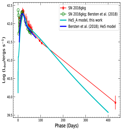
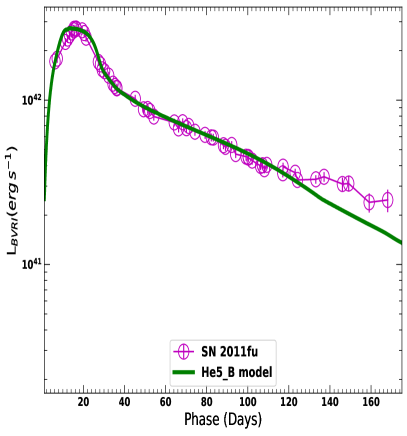
Figure 4.12: The results of 1-dimensional stellar evolution of models using MESA and their synthetic explosion using SNEC for SN 2016gkg and SN 2011fu. Left: Comparison of the quasi-bolometric light curve of SN 2016gkg with that obtained using SNEC by taking into account the ⁵⁶Ni and ⁵⁶Co decay model and keeping the parameters close to those of Bersten et al. (2018). Right: Result of a similar analysis for SN 2011fu.

Recent studies suggest the masses of possible progenitors of Type IIb CCSNe to be usually higher than 9 M_⊙, lying in the range 10–18 M_⊙ (Van Dyk et al., 2013; Folatelli et al., 2014; Smartt, 2015). However, there has been no direct observational evidence of an SN IIb arising from a ZAMS progenitor of $\lesssim 12$ M_⊙. The present analysis indicates that SN 2016iyc arises from the lower-mass end of the SN IIb progenitor channel. As part of our study, we also performed the 1-dimensional stellar evolutions of the possible progenitors of SN 2016gkg and SN 2011fu, and we simulated their hydrodynamic explosions in the next section to cover the range of faintest (SN 2016iyc), intermediate (SN 2016gkg), and highest (SN 2011fu) luminosity SNe in the comparison sample.

4.6 Stellar Modelling and Synthetic Explosions for SN 2016gkg and SN 2011fu

In this section, we perform hydrodynamic simulations of explosions from the possible progenitors of an intermediate-luminosity SN 2016gkg and the most-luminous SN 2011fu in the comparison sample to cover the higher end of the progenitor masses of SNe IIb. After modelling their progenitors using MESA, we simulate the synthetic explosions using SNEC and match the SNEC produced bolometric light curves with the observed ones.

To construct the bolometric light curve of SN 2016gkg, we used the recalibrated $BVRI$ KAIT data along with the data from the 3.6 m DOT at two epochs and incorporated SUPERBOL. The photometric data of SN 2016gkg in this work are presented in Table B.3 and Table B.4. Previously, Bersten et al. (2018) also used KAIT data calibrated from an older KAIT reduction pipeline. Figure B.4 shows the comparison between the KAIT data used by Bersten et al. (2018) and the recalibrated KAIT data. To construct the bolometric light curve of SN 2011fu, we make use of SUPERBOL as we did in earlier sections by incorporating the $BVRI$ data from Kumar et al. (2013).

To model the possible progenitor of SN 2016gkg, we closely follow the HE5 model from Bersten et al. (2018). Also, Morales-Garoffolo et al. (2015) suggests a nearly similar model for the possible progenitor of SN 2011fu. An 18 M_⊙ ZAMS progenitor mass is employed for both SNe. The modelling and explosion parameters are listed in Table B.1. Starting from the ZAMS, the model is evolved up to the stage where the core starts to collapse. The evolution of the model on the HR diagram is shown in the left panel of Figure 4.8. Various physical processes during the evolution on the HR diagram have been indicated. Also, the right-hand panel displays the variation of $T_{\rm core}$ with $\rho_{\rm core}$. It is indicated that during the last evolutionary phases, the core density and temperatures have reached over $10^{10}$ g cm^-3 and $10^{10}$ K, respectively. Such high core density and temperatures mark the onset of core collapse. The left panel of Figure 4.11 shows the mass fractions of various elements at the stage when the model has just reached the stage of Fe-core infall. As another piece of evidence for the onset of core collapse, we can see that the core is mainly composed of inert ⁵⁶Fe. The right-hand panel of Figure 4.11 shows the Kippenhahn diagram of the model for a period from the beginning of main-sequence evolution to the stage when the model is ready to be stripped.

Models He5_A and He5_B are used for SN 2016gkg and SN 2011fu, respectively. Although the parameters, including the ZAMS mass, metallicity, rotation, and overshoot parameter, are the same for these two models, different explosion parameters are employed using SNEC to simulate the synthetic explosions.

The left panel of Figure 4.12 illustrates the comparison of our hydrodynamic simulation of synthetic explosions for SN 2016gkg with the results of Bersten et al. (2018). The difference between the bolometric light curve from Bersten et al. (2018) and calculated using KAIT revised photometry are within the error bars. Our model could explain the bolometric light curve of SN 2016iyc very well. Furthermore, the right-hand panel of Figure 4.12 shows the comparison of the SNEC-calculated bolometric light curve with the observed quasi-bolometric light curve of SN 2011fu. The 1-dimensional stellar modelling of possible progenitors using MESA along with their hydrodynamic simulation of explosions using SNEC explain the observed light curves of SN 2016gkg and SN 2011fu very well. Now, we have performed the stellar modelling of the possible progenitors and the hydrodynamic explosions of SN 2016iyc, SN 2016gkg, and SN 2011fu to cover a range of faintest (SN 2016iyc), intermediate (SN 2016gkg), and highest (SN 2011fu) luminosity SNe in the comparison sample.

4.7 Discussion on Findings

Detailed photometric and spectroscopic analyses of the low-luminosity Type IIb SN 2016iyc are performed in this work. The extinction-corrected data of SN 2016iyc are used to construct the quasi-bolometric and bolometric light curves using SUPERBOL. Comparisons of the absolute $V$-band and quasi-bolometric light curves of SN 2016iyc with other well-studied SNe IIb indicate that SN 2016iyc lies toward the faint limit of this subclass. Low-luminosity SNe IIb with low ⁵⁶Ni production are thought to arise from progenitors having masses near the threshold mass for producing a CCSN.

Our study indicates that among the comparison sample in this work, SN 2016iyc has the smallest blackbody radius at any given epoch. This anomalous behaviour could be attributed to its low ejecta velocity.

Based on the low $M_{\rm ej}$ and the lowest intrinsic brightness among SNe in the comparison sample, 9–14 M_⊙ ZAMS progenitors are modelled as the possible progenitor of SN 2016iyc using MESA. The results of synthetic explosions simulated using STELLA and SNEC are in good agreement with the observed ones.

The 1-dimensional stellar modelling of the possible progenitor using MESA and simulations of hydrodynamic explosions using SNEC/STELLA indicate that SN 2016iyc originated from a (12–13) M_⊙ ZAMS progenitor, near the lower end of progenitor masses for SNe IIb. The models show a range of parameters for SN 2016iyc, including $M_{\rm ej}=$ (1.89–1.93) M_⊙ and $E_{\rm exp}=$ (0.28–0.35) $\times 10^{51}$ erg. We also put an upper limit of 0.09 M_⊙ on the amount of nickel synthesised by the SN. The pre-SN radius of the progenitor of SN 2016iyc is (240–300) R_⊙.

Stellar evolution of the possible progenitors and hydrodynamic simulations of synthetic explosions of SN 2016gkg and SN 2011fu have also been performed to compare the intermediate- and high-luminosity ends among well-studied SNe IIb using MESA and SNEC. The results of stellar modelling and synthetic explosions for SN 2016iyc, SN 2016gkg, and SN 2011fu exhibit a diverse range of mass of the possible progenitors for SNe IIb.

4.8 Summary and Conclusions

We performed detailed photometric and spectroscopic analyses of SN 2016iyc, a Type IIb SN discovered by LOSS/KAIT. The observed photometric properties of SN 2016iyc were unique in many ways: low luminosity, low ejecta mass, and small blackbody radius. Attempts to model the possible progenitor were made using the 1-dimensional hydrodynamic code MESA. As a part of the present work, hydrodynamic modelling of the synthetic explosion of an intermediate-luminosity Type IIb SN 2016gkg using recalibrated KAIT data and late-time data from the 3.6 m DOT, along with an optically very luminous Type IIb SN 2011fu, were also performed. The main results based on the present analysis are as follows.

1. Based on the low value of $M_{\rm ej}$, ZAMS stars having masses of 9–14 M_⊙ were adopted to model the possible progenitor of SN 2016iyc using MESA. The results of synthetic explosions simulated using SNEC and STELLA were in good agreement with observed properties for ZAMS progenitor masses of 12–13 M_⊙ having a pre-SN radius of (240–300) R_⊙. Thus, SN 2016iyc likely had a progenitor arising from the lower end of the progenitor mass channel of an SN IIb.
   

2. We concluded that the overall detailed hydrodynamic simulations of the explosions from various models showed a range of parameters for SN 2016iyc, including an $M_{\rm ej}$ of (1.89–1.93) M_⊙, an $E_{\rm exp}$ of (0.28–0.35) $\times 10^{51}$ erg, and an upper limit of $<0.09$ M_⊙ on the amount of nickel synthesised by SN 2016iyc.
   

3. Finally, 1-dimensional stellar evolution models of possible progenitors and the hydrodynamic explosions of SN 2016gkg and SN 2011fu were also performed to compare intermediate- and high-luminosity examples among well-studied SNe IIb. The results for SN 2016iyc, SN 2016gkg, and SN 2011fu showed a diverse range of mass [(12.0–18.0) M_⊙] for the possible progenitors of SNe IIb considered in this work. Discovery of more such events through survey projects in the near future should provide additional data with which to establish the lower mass limits of such explosions.

Chapter 5 Investigating the evolutions of Rotating, Population III star of 25 M_⊙ and the strength of Resulting Supernovae

5.1 Pop III Stars and their Impact in the Early Universe

Having comprehensively discussed the temporal and spectral properties of H-deficient Type Ib SNe in Chapter 3 followed by the detailed photometric and spectroscopic analysis of a Type IIb SN retaining an intermediate amount of H-envelope in Chapter 4, this Chapter discusses H-rich and H-deficient CCSNe together that originate from progenitors each starting with a mass of 25 M_⊙ at ZAMS and zero metallicity. The first generations of stars formed out of uncontaminated matter, initially comprised only of the first two stable elements, hydrogen and helium, from the periodic table, are considered population III (Pop III) stars.

Due to the insufficiency of coolants in the primordial gas, it is hypothesised that the Pop III stars were massive intrinsically (Silk, 1983; Tegmark et al., 1997; Bromm et al., 1999; Nakamura & Umemura, 2001; Abel et al., 2002; Brook et al., 2007; Salvadori et al., 2010; Hirano et al., 2015). However, there have been multiple studies to apprehend the possibility of the existence of Pop III stars having low masses. In recent simulations, it has been found that the formation of pristine, metal-free stars at low to intermediate masses could potentially be due to the fragmented accretion disks around massive Pop III protostars (Turk et al., 2009; Stacy et al., 2010; Hosokawa et al., 2011; Clark et al., 2011; Greif et al., 2012; Hirano et al., 2014, 2015; Stacy et al., 2016; Riaz et al., 2018; Wollenberg et al., 2020). On the-low mass Pop III stars, Ishiyama et al. (2016) have found that the Pop III stars having masses $<$ 0.8 M_⊙ would have longer lifetimes as compared to the cosmic time; therefore such low-mass stars could linger around to be detected in our Milky Way itself.

Further, Pop III stars were responsible for the enrichment of the early universe by spreading metals heavier than He through violent supernova (SN) explosions or possibly through sporadic mass losses due to vigorous stellar winds (Ferrara et al., 2000; Abia et al., 2001). The study by Chiaki et al. (2018) shows that a CCSN from a Pop III star could cause the minihalo to undergo internal-enrichment. This causes the metallicity to be -5 $\lesssim$ [Fe/H] $\lesssim$-3 in the recollapsing region. Thus, internal-enrichment caused by a CCSN from a Pop III star can explain the stars which are extremely metal-poor. In relatively recent work, the authors of Kirihara et al. (2020) have estimated the dose of heavy elements introduced by massive Pop III stars. In doing so, they considered the amount of heavy elements synthesised only from PISNe or CCSNe explosions of massive Pop III stars. They found that the heavy elements introduced by Pop III stars are usually much more than those from galaxies found in the low-density regions. Besides the above-mentioned studies involving Pop III stars, there have also been investigations to recognise the influence of Pop III stars on cosmic reionization (e.g., Haiman et al., 1997; Tumlinson & Shull, 2000; Barkana & Loeb, 2001; Ciardi et al., 2001; Bromm, 2013), and dust formation (Todini & Ferrara, 2001).

There have been multiple studies to understand the evolution of the Pop III stars. Marigo et al. (2003) and Ekström et al. (2008) have studied the evolution of Pop III stars by assuming solid-body and differential rotation, respectively. Heger & Woosley (2010) have discussed the nucleosynthesis and evolutions of non-rotating Pop III stars. They also generated the light curves of the resulting transients from the non-rotating models corresponding to different explosion energies. Yoon et al. (2012) have discussed the evolution of massive Pop III stars having masses in the range of [10 – 1000] M_⊙ and have investigated the consequences of including rotation and magnetic fields. Due to the chemically homogeneous evolution, the rapidly rotating high-mass stars could result in a class of energetic transients, including Type Ib/c SNe, GRBs, HNe, and PISNe. In their work, Yoon et al. (2012) have prepared a phase diagram in the plane of mass and rotational velocity at ZAMS and discussed the culminating fates of Pop III stars. The authors of Windhorst et al. (2018) have investigated the evolutions of non-rotating Pop III stars in the mass range of [1 – 1000] M_⊙ considering no mass loss and have also discussed chances of the observability of an individual Pop III star. In recent work, Murphy et al. (2021) have studied a grid of Pop III models having masses in the range of [1.7 – 120] M_⊙ and explored the effect of changing the initial rotational velocity from 0 to 40 per cent of critical rotational velocity.

Taking such studies one step further, in this work, we study the entire evolution (from ZAMS up to the stage of the onset of core collapse) of a 25 M_⊙ Pop III star and investigate the effect of rotation on the final fates. Following the phase diagram in Yoon et al. (2012), the resulting supernovae (SNe) from a 25 M_⊙ ZAMS star will either be weak Type II or Type Ib/c depending upon the initial rotations. For the first time in this work, we have evolved the rotating and non-rotating Pop III models together up to the onset of core collapse. We further performed the hydrodynamic simulations of their synthetic explosions, showing the light curves of resulting transients.

We have divided this Chapter into four sections. After providing a brief introduction of literature in Section 5.1, we discuss the numerical setups and physical properties of the models in Section 5.2. The numerical setups to simulate the hydrodynamic explosion of models are discussed in Section 5.3. Finally, the major outcomes from the entire evolutions of the models, along with their synthetic explosions, are discussed in Section 5.4. In this Section, we also provide the implications and discussions of the simulation results presented in the underlying work.

5.2 Stellar Evolution Using MESA

5.2.1 Numerical setups

We employ one of the state-of-the-art and 1-dimensional stellar evolution codes, MESA to perform the stellar evolutions of 25 M_⊙ ZAMS stars with zero metallicity (Z = 0.00) and different initial rotations. In this simulation work, we have utilised the MESA version r22.05.1 (Paxton et al., 2011, 2013, 2015, 2018). We start with a non-rotating, zero metallicity model and increase the angular rotational velocity ($\Omega$) in units of 0.2 times the critical angular rotational velocity ($\Omega_{\rm crit}$) up to $\Omega$ / $\Omega_{\rm crit}$ $=$ 0.8. Following Paxton et al. (2013), the critical angular rotational velocity is expressed as $\Omega_{\rm crit}^{2}=(1-L/L_{\rm edd})GM/R^{3}$, where $L_{\rm edd}$ is the Eddington luminosity. As specified in the default MESA setups, when the ratio of the luminosity from nuclear processes and the overall luminosity of the model at a particular stage reaches 0.4 (set by Lnuc_div_L_zams_limit = 0.4 in MESA), the model is assumed to have reached ZAMS. Adopting the Ledoux criterion, convection is modelled utilising the mixing theory of Henyey et al. (1965). We have adopted a mixing-length-theory parameter ($\alpha_{\rm MLT}$) $=$ 2.0 in the whole analysis. Following Langer et al. (1985), semi-convection is modelled by setting an efficiency parameter of $\alpha_{\mathrm{sc}}$ = 0.01. To model the thermohaline mixing, we follow Kippenhahn et al. (1980) by fixing the efficiency parameter to $\alpha_{\mathrm{th}}$ = 2.0. To model the convective overshooting, we use the diffusive approach as presented in Herwig (2000) and set $f=0.004$ and $f_{0}=0.001$ for all convective cores and shells. The stellar winds from rotating Pop III stars are also theorised to make contributions to the enrichment of the early universe with heavy metals, so to model the stellar winds of the Pop III stars in our study, we use the ’Dutch’ wind scheme (Glebbeek et al., 2009) and set the scaling factor ($\eta$) to 0.5. This wind scheme incorporates the outcomes from multiple works for different situations, with m_H representing the surface mass fraction of hydrogen, (a) when the effective temperature, T${}_{\rm eff}>10^{4}$ K along with m_H being greater than 0.4, the outcomes of Vink et al. (2001) are used; (b) when T${}_{\rm eff}>10^{4}$ K combined with the m_H being lesser than 0.4, the results of Nugis & Lamers (2000) are used; and finally (c) the wind scheme presented in de Jager et al. (1988) is used in MESA for the condition with T${}_{\rm eff}<10^{4}$ K.

Starting from the pre-ZAMS, the 1-dimensional stellar evolutions of the Pop III models are performed till they reach the stage of the onset of the Iron core collapse. The onset of core collapse is marked when the infall velocity of the Iron core exceeds the specified Iron core infall velocity limit of 100 km s^-1 (set by fe_core_infall_limit = 1d7 in MESA). In this work, the models have been named in a way that they contain the pieces of information, including the ZAMS mass, metallicity, and rotation ($\Omega$ / $\Omega_{\rm crit}$ indicated by “Rot”). For example, the model M25_Z0.00_Rot0.0 indicates a 25 M_⊙ ZAMS star with Z = 0.00, and $\Omega$ / $\Omega_{\rm crit}$ = 0.0. For comparison purposes, we have also performed the evolution of a solar metallicity (Z = 0.02) model with the same ZAMS mass of 25 M_⊙.

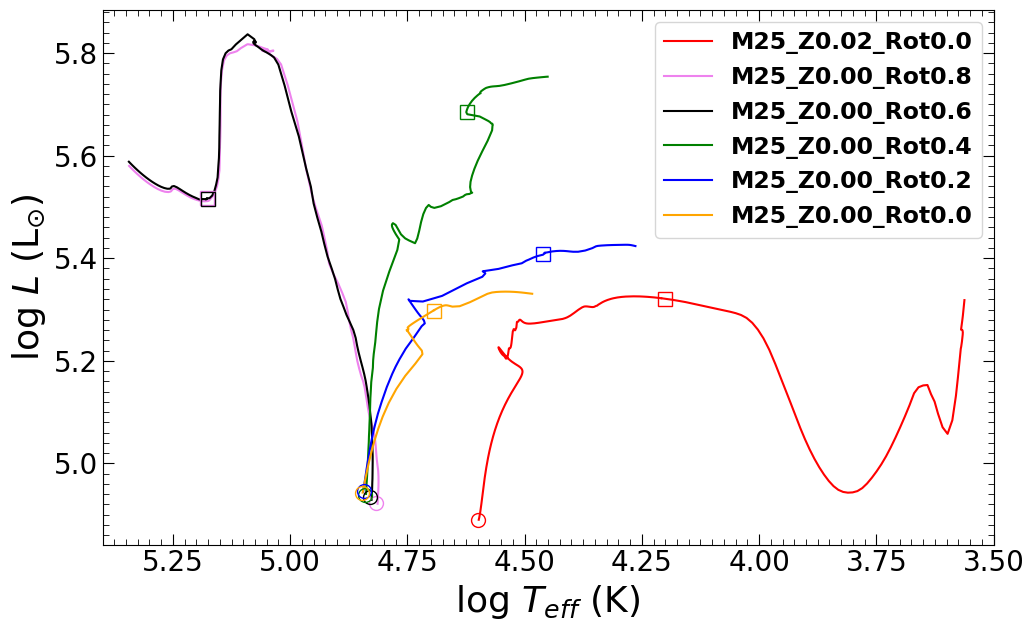
Figure 5.1: Evolution of the Pop III models having different rotations on the HR diagram. The arrivals of the models on ZAMS are shown by hollow circles, while the core-He exhaustion stages of the models have been marked by hollow squares. The solar metallicity (Z = 0.02) model evolutionary track has also been shown for comparison.

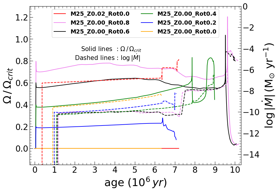
Figure 5.2: The evolution of angular rotational velocity ($\Omega$) in units of critical angular rotational velocity ($\Omega_{\rm crit}$) along with corresponding mass loss rate (log $|\dot{M}|$) evolution.

5.2.2 Physical properties of the models

Figure 5.1 displays the evolutions of Pop III models with 25 M_⊙ ZAMS mass each, on the Hertzsprung–Russell (HR) diagram along with a similar ZAMS mass model having solar metallicity (Z = 0.02) for comparison purposes. Compared to a solar metallicity model, the Pop III models reach the ZAMS at higher effective temperatures ($T_{\rm eff}$) but show nearly similar ZAMS luminosities. Thus, the Pop III models are bluer than the solar metallicity model. Among Pop III models, at ZAMS, the models with higher initial angular rotational velocities possess lower luminosities and lower effective temperatures; a well-known effect of rotation as mentioned in Ekström et al. (2008). It is also evident from this figure that beyond ZAMS, the models with higher initial angular rotational velocities possess higher luminosities and higher effective temperatures as well for most of their evolutionary paths. Similar results were also obtained in the case of Yoon et al. (2012).

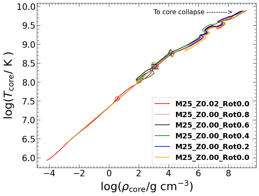
Figure 5.3: The variations of core-temperature ($T_{\rm core}$) vs core-density ($\rho_{\rm core}$) curves throughout the course of evolution of the models on the HR Diagram. The arrival on the ZAMS, exhaustion of core-He burning, and exhaustion of core-C burning have been marked by hollow circles, squares, and diamonds, respectively.

Figure 5.2 shows the variations of $\Omega$ / $\Omega_{\rm crit}$ and corresponding mass loss rates (log $|\dot{M}|$) as the models evolve up to the stage of the onset of core collapse. Initially, the models touch the specified $\Omega$ / $\Omega_{\rm crit}$ values and then settle to new $\Omega$ / $\Omega_{\rm crit}$ values as they evolve further. This shows that a perturbation imposed on an equilibrium model experiences a transient response before the system settles into a new equilibrium configuration. During the last evolutionary stages, the rapidly rotating models (with $\Omega$ / $\Omega_{\rm crit}$ = 0.6 and 0.8) show chaotic rotations exceeding the critical rotational velocities which are responsible for the dynamic events to occur as indicated by corresponding heavy mass loss rates during these phases. Our rapidly rotating massive Pop III stars dredge up a large amount of CNO elements up to the surface during the core-He burning stage. It dramatically increases the surface metallicity, which eventually strongly boosts the radiative mass loss through a mechanism similar to that discussed in Hirschi (2007). Thus, the rapidly rotating models are significantly stripped compared to the slow- or non-rotating models. We have also shown the Kippenhahn diagram for one slow-rotating model (M25_Z0.00_Rot0.2) and one rapidly rotating model (M25_Z0.00_Rot0.8) in Figure C.1. A few more important physical properties, including radii and effective temperatures ($T_{\rm eff}$) at various stages, are listed in Table 5.1.

The overall variations of the core-density ($\rho_{\rm core}$) vs core-temperature ($T_{\rm core}$) curves for the entire evolutions of the models up to the onset of core collapse are shown in Figure 5.3. The arrival of the models on ZAMS, the exhaustion of core-He burning phases, and the exhaustion of core-C burning stages have been indicated by the hollow circles, squares, and diamonds, respectively. Compared to a solar metallicity model, the Pop III models ignite the H-burning in their respective cores at higher $\rho_{\rm core}$ and $T_{\rm core}$, which is due to the lack of CNO elements in Pop III stars needed to ignite the CNO cycle (Ekström et al., 2008). During the last evolutionary stages, all the models have exceeded the core temperatures of $\sim$10^9.9 K; the perfect condition for the cores to collapse under their own gravity. Thus, the models have now reached the stage of the onset of core collapse.

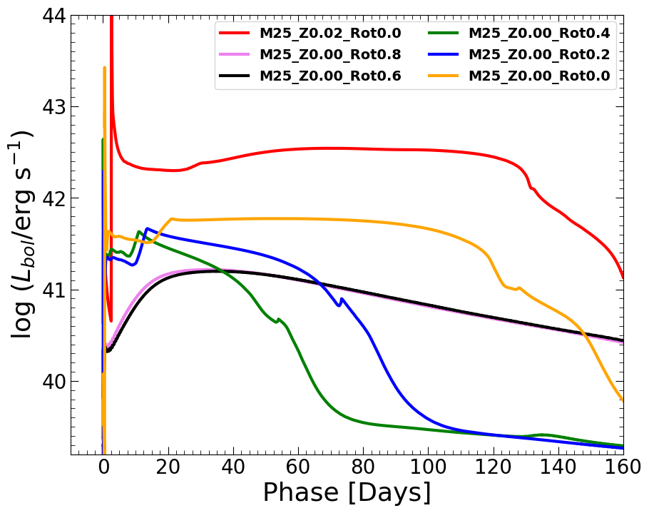
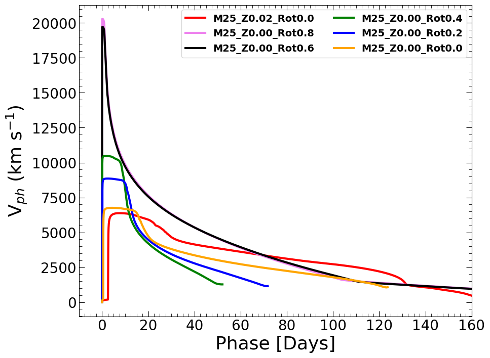
Figure 5.4: Left: The bolometric luminosity light curves resulting from the synthetic explosions of models using SNEC. Right: Corresponding photospheric velocity evolutions. Results of the non-rotating solar metallicity model are also shown for comparison.

Table 5.1: The ZAMS and pre-SN properties of the Pop III models using MESA along with the SNEC explosion parameters.

		ZAMS					pre-SN			Explosion
Model Name	$M_{\rm ZAMS}^{a}$	$T_{\mathrm{eff}}$	$R_{\mathrm{ZAMS}}^{b}$	$L_{\rm ZAMS}^{c}$	$M_{\rm pre-SN}^{d}$	$T_{\mathrm{eff}}$	$R_{\mathrm{pre-SN}}^{e}$	$L_{\rm pre-SN}^{f}$	$M_{\mathrm{c}}^{g}$	$M_{\mathrm{ej}}^{h}$	$M_{\mathrm{Ni}}^{i}$	$E_{\mathrm{exp}}^{j}$
	(M⊙)	K	(R⊙)	(L⊙)	(M⊙)	K	(R⊙)	(L⊙)	(M⊙)	(M⊙)	(M⊙)	($10^{51}$ erg)
M25_Z0.00_Rot0.0	25.0	70069	2.01	4.94	24.99	10319	195	5.58	1.70	23.29	0.001	1.0
M25_Z0.00_Rot0.2	25.0	69877	2.02	4.94	24.99	17216	57	5.42	2.00	22.99	0.001	1.0
M25_Z0.00_Rot0.4	25.0	68882	2.07	4.94	24.96	29784	32	5.87	1.80	23.16	0.001	1.0
M25_Z0.00_Rot0.6	25.0	67069	2.16	4.93	11.94	140668	1.5	5.90	2.10	9.84	0.05	1.0
M25_Z0.00_Rot0.8	25.0	65107	2.26	4.91	11.79	175858	0.6	5.53	2.10	9.69	0.05	1.0
M25_Z0.02_Rot0.0	25.0	3962	5.91	4.88	22.64	3623	1219	5.36	1.90	22.74	0.001	1.0

^aMass at ZAMS. ^bProgenitor radius at ZAMS, ^cLuminosity at ZAMS, ^dFinal mass of pre-SN model, ^epre-SN phase radius, ^fpre-SN phase luminosity, ^gMass of the central remnant in simulation, ^hEjecta mass, ⁱAmount of synthesised nickel used in the explosion, ^jExplosion energy.

5.3 Synthetic Explosions Using SNEC

Once the models have reached the stage of core collapse marked by the infall velocity exceeding the specified Iron-core infall velocity, the outputs of MESA in appropriate forms are provided as input to SNEC (Morozova et al., 2015). SNEC is a 1-dimensional Lagrangian hydrodynamic code that simulates the synthetic explosions of the stellar models at the stage of the onset of their core collapse. SNEC solves the radiation energy transport equations within the flux-limited diffusion approximation to simulate the explosions.

Further, in this work, to simulate the synthetic explosions of the models which have already arrived at the stage of the onset of core collapse, we closely follow the setups of Ouchi & Maeda (2019) along with Aryan et al. (2021b, 2022c) for SNEC. However, the major changes are summarised here. First, for each model, the innermost mass $M_{\rm c}$ representing the mass of the central remnant is excised before the explosion by assuming that the model will finally collapse to form an NS. The central remnant mass is decided by the final mass of the Iron-core when the model has reached the stage of the onset of core collapse. Further, a set of 800 grid cells are used to simulate the synthetic explosion of the model. With 800 grid cells, the light curves and photospheric velocities of the resulting SN from simulations are very well converged in the interested domains of time. The explosion of each model is simulated as thermal bomb by adding $E_{\rm exp}$ amount of energy for a duration of 0.1 s in the inner 0.1 M_⊙ section of the model. As discussed in Morozova et al. (2015), SNEC lacks a nuclear-reaction network; thus, the synthesised amount of nickel (⁵⁶Ni) in an SN is decided and fixed by the individual user. For each model, an amount of ⁵⁶Ni specified by corresponding $M_{\rm Ni}$ in Table 5.1, is distributed between the excised central remnant mass ($M_{\rm c}$) cut and the chosen mass coordinate which is close to the outer surface of the selected model. For models with $\Omega$ / $\Omega_{\rm crit}$ $\leq$ 0.4, the amount of ⁵⁶Ni is set to 0.001 M_⊙ while the remaining models with heavy rotations and suffering significant mass losses, the amount of ⁵⁶Ni is set to 0.05 M_⊙. Choosing a slightly greater amount of $M_{\rm Ni}$ for stripped models is followed by Afsariardchi et al. (2021). The ejecta mass ($M_{\rm ej}$) for each CCSN is estimated by finding the difference between the pre-SN mass ($M_{\rm Pre-SN}$) and $M_{\rm c}$. The detailed explosion parameters are listed in Table 5.1.

Finally, the $UBVRI$ -bands light curves generated through synthetic explosions are shown in Figure C.2. As shown in this figure, the slow-rotating models (i.e., models M25_Z0.00_Rot0.0, M25_Z0.00_Rot0.2, M25_Z0.00_Rot0.4, and the solar metallicity model M25_Z0.02_Rot0.0) retaining a significant amount of their outer H-envelope result into Type II CCSNe. In contrast, the rapidly rotating models result in CCSNe Type Ib/c. These results are also complementing the results as predicted in the phase diagram of Yoon et al. (2012) (in Figure 12). In Figure C.2, a few important simulation results of the H-rich Pop III CCSNe (i.e. models with $\Omega$ / $\Omega_{\rm crit}$ $\leq$ 0.4) are also displayed; First, the peak magnitudes of the shock breakout (SBO) features from these models are much fainter than a typical solar metallicity H-rich CCSN; second, the absolute magnitudes of the plateau of the H-rich Pop III CCSNe are at least 1.5 magnitudes fainter than the solar metallicity H-rich CCSN; thus the H-rich Pop III CCSNe are pretty faint within the considered limits of $E_{\rm exp}$ and $M_{\rm Ni}$ in this study. The effect of bolometric light curves becoming less luminous as metallicity decreases has been explored in Kasen & Woosley (2009) and Paxton et al. (2018). The primary cause of this behaviour is associated with the smaller pre-SN radius and less total mass loss as an effect of lower metallicity. However, in their work, they have not calculated the light curves corresponding to Z = 0.00; and the third, surprisingly, although the pre-SN radius of the non-rotating H-rich Pop III model is much smaller than a non-rotating solar metallicity H-rich model, the earlier model shows almost a similar plateau duration. The non-rotating solar model has a larger pre-SN radius compared to the M25_Z0.00_Rot0.0 model, but the latter has a more massive H-envelope. From Figure C.3, the M25_Z0.02_Rot0.0 model has an H-envelope starting from a mass coordinate, m(M_⊙)$\sim$8 M_⊙ while the M25_Z0.00_Rot0.0 has a more-massive H-envelope starting from m(M_⊙)$\sim$5 M_⊙. Thus, the presence of extra hydrogen could be responsible for the increased plateau duration in the non-rotating Pop III model. Finally, the rapidly rotating H-less Pop III models result into much fainter Type Ib/c SNe. These explosions are fainter because of the less explosion energy (and an M_Ni of 0.05 M_⊙) considered in our study. With higher explosion energies and more nickel production, they might result in more luminous SNe or HNe (Nomoto et al., 2013). SNEC could also produce the bolometric luminosity light curves and the corresponding photospheric velocity evolutions for all the models as shown in the left and the right panels of Figure 5.4, respectively. In the left panel, the bolometric light curves of the Pop III CCSNe display a similar behaviour as earlier in the case of $UBVRI$ -bands light curves comparison with the solar metallicity model. In the right panel, as expected, the stripped models display higher photospheric velocities compared to the H-rich models.

5.4 Results and Discussion

In this work, we have performed the 1-dimensional stellar evolutions of Pop III models up to the stage of the onset core collapse and then simulated their synthetic explosions. Utilising the 1-dimensional simulations performed in this work, we summarise our findings below:

1. The peak absolute magnitudes of the SBO features of Pop III CCSNe are much smaller than that of a CCSN, resulting from a solar Type model with similar ZAMS mass.

2. The H-rich CCSNe from Pop III models are fainter than the H-rich SN resulting from a solar metallicity model. The plateau magnitudes of Pop III star H-rich CCSNe are at least 1.5 magnitudes fainter than the latter. In the earlier epochs, the stripped CCSNe from Pop III models are much fainter than SNe resulting from H-rich Pop III models.

3. One of the most intriguing results from our simulations is that although the pre-SN radius of a non-rotating H-rich Pop III model is much smaller than a non-rotating H-rich solar Type model, both models show nearly similar plateau durations. One of the reasons for the increased plateau duration, despite a relatively smaller pre-SN radius in non-rotating Pop III CCSNe, could be associated with the increased amount of hydrogen mass.

4. Among the discussed Pop III models, SN resulting from the non-rotating H-rich model is the brightest. It has a nearly constant absolute magnitude of around -16.5 mag in the V-band for the plateau phase. This would correspond to an apparent magnitude of $\sim$35.5 mag at a redshift of $z$ = 10 (using the cosmology of a Hubble constant, H₀ = 73, $\Omega_{\rm M}$ = 0.3, and $\Omega_{\rm vac}$ = 0.7). Currently, no ground- or space-based observatory can go this faint to detect a Pop III CCSN resulting from an individual star; however, with the major advancement in observational technologies having large diameters could possibly detect such events in the near future.

5. Thus, through our work, we find that within the considered limits of explosion energies and nickel masses, these transient events are very faint, making it difficult for them to be detected at high redshifts.

Chapter 6 Evolution of a non-rotating 100 M_⊙ ZAMS star resulting in to Type IIP-like supernovae

6.1 Final Fates of Very Massive Stars

Chapters 3, 4, and 5 discuss the properties of canonical CCSNe arising from progenitors having ZAMS masses of 25 M_⊙ or less. However, in this Chapter, we present the pure simulation-based results of the stellar evolution of a 100 M_⊙ ZAMS progenitor star and discuss the resulting transients.

In this work, we take a 100 M_⊙ ZAMS star with metallicity, Z = 0.01, and evolve it up to the stage of core-collapse, and finally, the synthetic explosions are simulated. Depending on the mass loss rate, rotation, and even on metallicity, such a heavy progenitor could result in various transients, including PISN, PPISN, Type IIp, Type IIn, Type Ibn, and Type Icn SNe also (Sukhbold et al., 2016; Woosley, 2017). The numerical simulations of such heavy progenitors are always a challenging task. With the mass loss and rotation included, the simulations are further complicated. The Type IIp SNe progenitors suffer minimal mass loss (as they retain almost all of their H-envelope) and possess (very) low rotation. Thus, to keep things simple yet close to reality, we try to model a massive ZAMS progenitor that can result in a Type IIP-like SN. One very recent study by Nicholl et al. (2020) indicates a total (SN ejecta + CSM) mass likely exceeding 50–100 M_⊙ for a Type II superluminous SN 2016aps. Attempts are underway to simulate such massive progenitors with much lower metallicities close to zero and even models with zero metallicity to understand the internal structure and resulting transients in the future. Although a few studies have been performed in this direction by (among others) Ohkubo et al. (2006), such studies are going to be extremely useful in understanding the final fates of massive primordial stars. The primary reason to choose a 100 M_⊙ ZAMS progenitor is that the mass ranges, including such heavy progenitors, are least explored. Only a handful of studies (eg. Sukhbold et al., 2016; Woosley, 2017) have been performed which discuss the evolution and final fates of such massive zero-age main-sequence progenitors. This study is a preliminary step to enhance our understanding of CCSNe originating from very high mass progenitors. Further, as mentioned above, a recent study by Nicholl et al. (2020) indicates a total (SN ejecta + CSM) mass exceeding 50–100 M_⊙, so our study is also going to be important to look into the progenitors of such events. Moreover, in the coming TMT, ELT and other large telescopes, such massive stars are likely to be discovered; thus, it will always be an interesting task to compare the simulations with the actual observations. All the analyses performed in this work make use of publicly available tools. A very nice review has been provided (among others) in Aryan et al. (2021a) depicting the usefulness of publicly available tools and how these tools can be a boon to the transient community.

This Chapter has been divided into six sections. The basic assumptions and methods of modelling the 100 M_⊙ progenitor have been discussed in section 6.2, thereafter the properties and parameters to synthetically simulate the explosions are discussed in section 6.3. The results of synthetic explosions have been discussed in section 6.4. Later, we discuss the major outcomes of our studies in section 6.5 and provide our concluding remarks in section 6.6.

6.2 1-dimensional stellar evolution of the 100 M_⊙ ZAMS progenitor using MESA

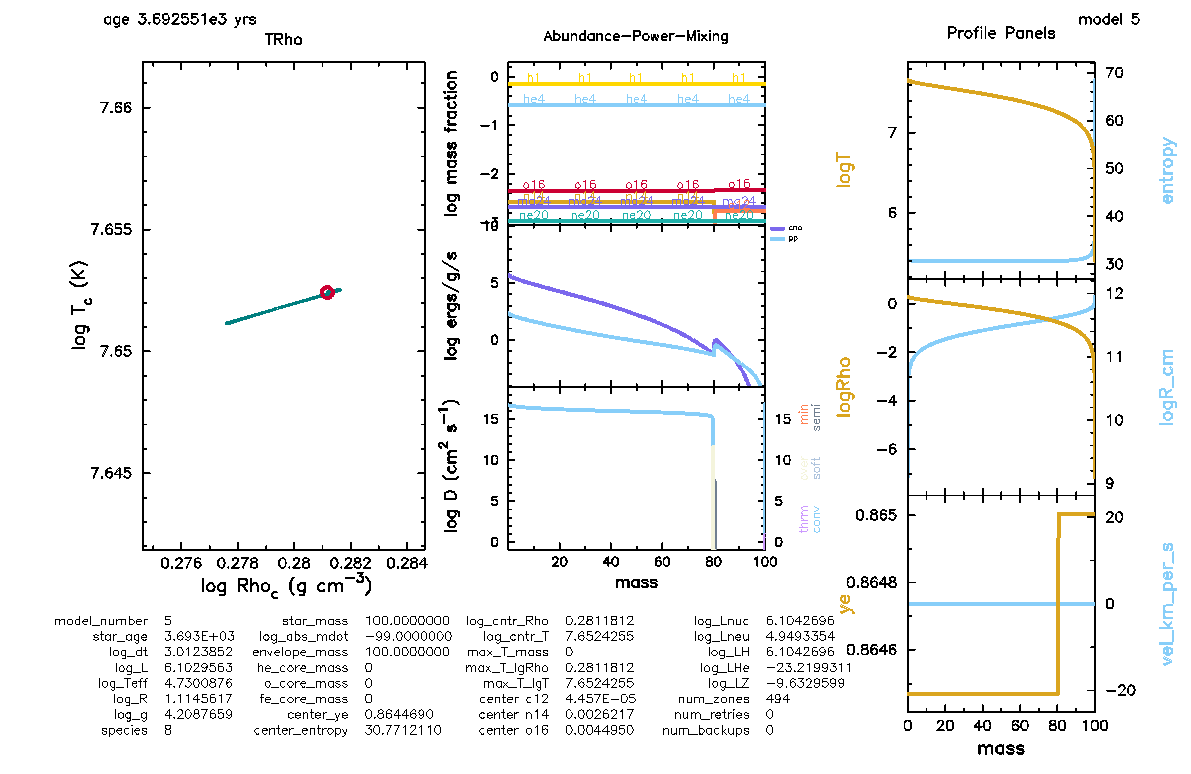
Figure 6.1: The physical condition and chemical engineering of our model when it has just arrived on the ZAMS. This figure is one of the many figures generated by MESA while the evolution of the models through various evolutionary phases.

In this work, we have taken a 100 M_⊙ ZAMS progenitor and evolved it up to the onset of core-collapse using MESA (version r11701). For this purpose, we used the default example_make_pre_ccsn directory available in MESA. Most of the settings closely follow Aryan et al. (2021b) and Pandey et al. (2021) with only a few minor deviations. We do not consider rotation and assume an initial metallicity of Z = 0.01. Convection is modelled using the mixing theory of Henyey et al. (1965) by adopting the Ledoux criterion. We set the mixing-length parameters to $\alpha$ = 3.5 in the region where the mass fraction of hydrogen exceeds 0.5 and set it to 1.5 in the other regions. Semi-convection is modelled following Langer et al. (1985) with an efficiency parameter of $\alpha_{\mathrm{sc}}$ = 0.01. For the thermohaline mixing, we follow Kippenhahn et al. (1980), and set the efficiency parameter as $\alpha_{\mathrm{th}}$ = 2.0. We model the convective overshooting with the diffusive approach of Herwig (2000), with $f$= 0.004 and $f_{0}$ = 0.001 for all the convective core and shells. We do not consider the presence of any strong stellar winds and hence consider no progenitor moss loss before the core collapse.

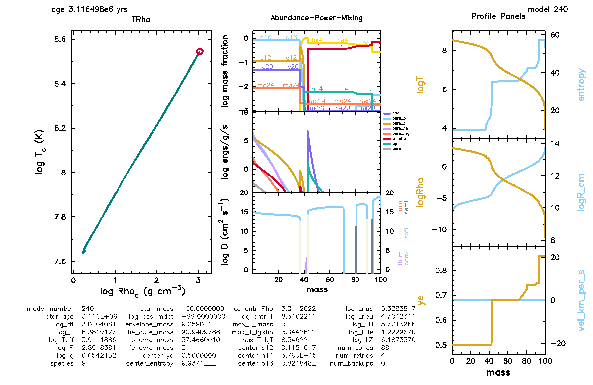
Figure 6.2: Same as fig. 6.1, but at the stage when the model has evolved through the main sequence and has become red supergiant.

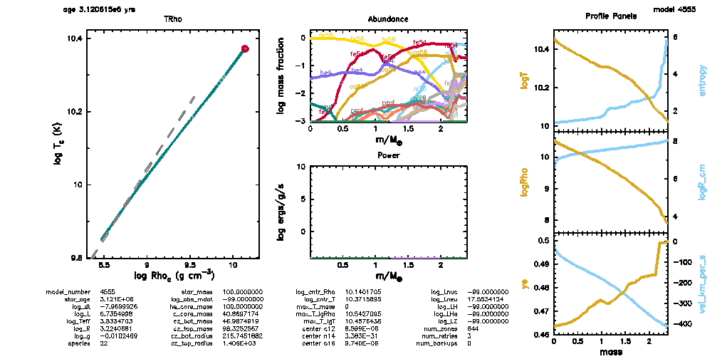
Figure 6.3: A glimpse of the physical and chemical structure of our model star just when the Iron-core infall has been achieved. We could see that the core-temperature and core-density have reached in excess of $10^{10}$ K and $10^{10}$ g cm^-3 respectively, which are supposed to be the perfect conditions for the core to collapse.

Further, we briefly explain the evolution of our models through the various stages. Landing on the ZAMS, our model evolves through the main-sequence, becomes supergiant, and finally approaches its death by developing an inert Fe-core in its centre. Figure 6.1 displays the physical condition and chemical engineering of our model when it has just landed on the main sequence. The arrival of our model on the main sequence is marked by the control parameter Lnuc_div_L_zams_limit, which checks the ratio of luminosity due to nuclear reactions and total luminosity at ZAMS. Once this ratio is $\sim$ 0.8, the onset of the main-sequence phase is marked. The leftmost panel of figure 6.1 shows the variation of the core-temperature (log T_c) and core density (log Rho_c) as the model evolves in time. On the beginning of main-sequence, the log T_c is $\sim$ 7.65 K and log Rho_c is $\sim$ 0.281 g cm^-3. The top plot in the middle panel of figure 6.1 displays the mass fraction of various elements present in the star. We can see that as the model has just arrived on the main-sequence, the fractions of H and He are much larger than any other heavy metals depending on the metallicity of our model. The middle plot in the middle panel of figure 6.1 shows the specific luminosity corresponding to the various processes inside the star. It can be seen that only two processes have kicked in as our model star is just beginning its journey through the main-sequence. The bottom plot in the middle panel shows the variation of the kinematic viscosity inside our model star. Now the rightmost panel of figure 6.1 shows various physical properties of our model star. Here, the topmost plot shows the variation of temperature and entropy with the mass coordinate, the middle plot shows the variation of density (logRho) and radius (logR_cm) of the model star with the mass coordinate, and finally, the bottom plot shows the variation of baryon fraction (ye) and convectional velocity (vel_km_per_s) inside the star.

The figure 6.2 shows similar properties as in figure 6.1, but at a stage when our model star has evolved through main-sequence and has become a supergiant. The leftmost panel in figure 6.2 shows that now the core temperature and density have risen considerably. Here, the top plot in the middle panel of figure 6.2 indicates the presence of heavier elements near the core while H and He are present in the envelope towards the higher mass coordinates. The middle plot in the middle panel of figure 6.2 shows that multiple energy generation processes have kicked in, while the bottom plot shows the further variation of kinematic viscosity inside our model star. Now, the rightmost panel of figure 6.2 depicts the variation of various physical parameters. From the radius plot, we can see that the model star has swollen up to $\sim$ 10¹⁴ cm, which is roughly around 1400 R_⊙ while from the temperature plot, we can see that the temperature (logT plot) near the surface is $\sim$ 10000 K. Such radius and temperature clearly indicate that our model is currently in the supergiant phase.

Finally, figure 6.3 shows similar properties but at a stage when the core of our model star is about to collapse. The leftmost panel of figure 6.3 shows the log T_c and log Rho_c have reached in excess of 10¹⁰ K and 10¹⁰ gm cm^-3 respectively. Such core temperatures and core densities are thought to be the perfect conditions for the core to undergo collapse. Thus, the core of our model star is about to collapse. The mass fraction and specific luminosity plots in the middle panel of figure 6.3 also depict perfect conditions for the core to collapse. In the mass fraction plot, a very high fraction of ⁵⁶Fe is seen, which indicates that the model star has developed an inert Fe-core, also in the specific luminosity plot, the absence of any energy generation process is seen. The plots in the rightmost panels of figure 6.3 show the physical properties of the inner–core regions. All these plots indicate the arrival of the stage of core collapse.

Post core-collapse, our model is evolved from a few seconds after the central explosion triggered by core-collapse to a time just before the outgoing shock reaches the stellar surface as discussed in Paxton et al. (2018). For this purpose, the default directory example_ccsn_IIp from MESA is used.

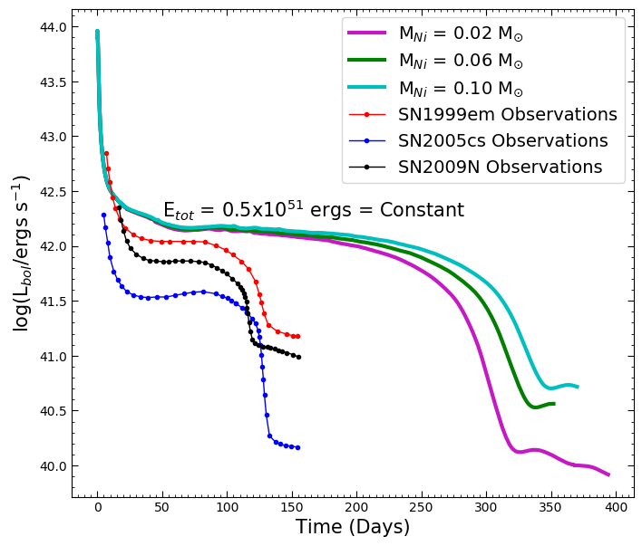
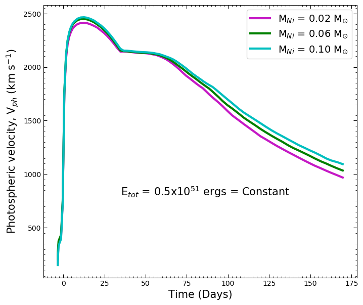
Figure 6.4: Results of the synthetic explosions simulated by STELLA, for comparison of the plateau phase, the bolometric light curves of three normal Type IIP SNe, namely SN1999em, SN2005cs, and SN2009N have also been plotted. The explosion energy has been kept fixed at 0.5$\times$10⁵¹ erg and the nickel mass is varied to 0.10 M_⊙, 0.06 M_⊙, and 0.02 M_⊙. Left: The behaviour of the bolometric light curve by the variation of nickel mass with the explosion energy kept constant has been displayed. The duration of the plateau increases with the increase in nickel mass. Right: The effect on the photospheric velocity when the nickel mass is varied, and the explosion energy is kept constant. Minimal changes are seen in the photospheric velocities.

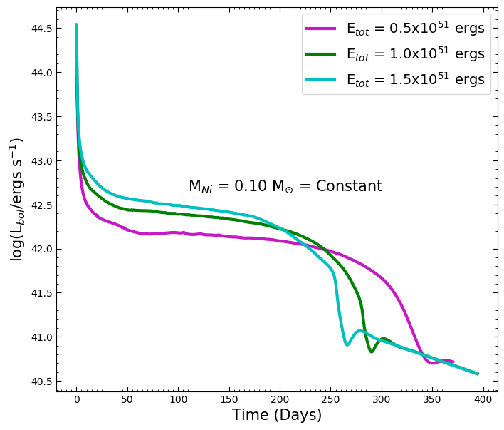
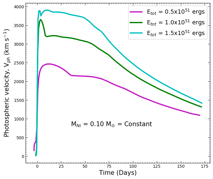
Figure 6.5: Results of the synthetic explosions simulated by STELLA. The nickel mass has been kept fixed to 0.10 M_⊙ and the explosion energy is varied to 0.5$\times$10⁵¹ erg, 1.0$\times$10⁵¹ erg and, 1.5$\times$10⁵¹ erg. Left: The behaviour of the bolometric light curve by the variation of explosion energy with the nickel mass kept constant has been displayed. The overall plateau luminosity increases with an increase in explosion energy, while the plateau duration decreases with an increase in explosion energy. Right: The effect on the photospheric velocity when the explosion energy is varied, and the nickel mass is kept constant. The photospheric velocities increase with the increase in explosion energy.

6.3 Synthetic Explosions Using STELLA

The output of MESA when the shock has reached just before the stellar surface, is fed as input to STELLA, which is a hydrodynamic code used to simulate the energetic CCSN explosions by evolving the model through shock-breakout. It solves the radiative transfer equations in the intensity momentum approximation in each frequency bin. In MESA, STELLA is run using 40 frequency groups, which is enough to produce spectral energy distribution, but insufficient to produce spectra. The opacity is computed based on over 153,000 spectral lines from Kurucz & Bell (1995) and Verner et al. (1996). To calculate the overall opacity, the code uses 16 species, which include H, He, C, N, O, Ne, Na, Mg, Al, Si, S, Ar, Ca, a sum of stable Fe and radioactive ⁵⁶Co, stable Ni and radioactive ⁵⁶Ni. The expansion opacity formalism from Eastman & Pinto (1993) is used to compute the line opacity by considering the effect of high-velocity gradients. The photo-ionization, electron scattering, and free-free absorption are also the sources of opacity that are included. Local thermodynamic equilibrium (LTE) is assumed in the plasma so that the Boltzmann-Saha distribution for ionization and level populations can be used. No nuclear networks except radioactive decay of ⁵⁶Ni to ⁵⁶Co which further decays to ⁵⁶Fe, are used. The energy from the radioactive decay of ⁵⁶Ni and ⁵⁶Co is deposited into positrons and gamma-photons. This energy is treated in a one-group transport approximation as suggested by Swartz et al. (1995).

In STELLA, a Lagrangian co-moving grid is used to solve the 1-dimensional equations for mass, momentum, and total energy. The artificial viscosity comprising of the standard von Neumann artificial viscous pressure is used for stabilising solution (Von Neumann & Richtmyer, 1950) and a so-called cold artificial viscosity is used to smear shocks (Blinnikov & Panov, 1996). So, STELLA enables one to properly compute the shock propagation along the ejecta and the shock breakout event. The coupled equations of radiation hydrodynamics are solved through an implicit high-order predictor–corrector procedure based on the methods of Brayton et al. (1972) (more details in Blinnikov & Panov 1996).

Our STELLA calculations include the synthetic explosions of a 100 M_⊙ ZAMS progenitor by assuming a set of explosion energies (E_tot) and nickel masses (M_Ni). The radioactive decay of ⁵⁶Ni and ⁵⁶Co powering mechanism has been employed in STELLA. We explored the effect on the bolometric light curve and photospheric velocity by changing one variable out of (E_tot) and (M_Ni) and keeping the other constant. In the first case, the explosion energy is kept constant to 0.5$\times$10⁵¹ erg while the nickel mass is changed to 0.10 M_⊙, 0.06 M_⊙, and 0.02 M_⊙. The masses of the central remnants for these cases were $\sim$41 M_⊙. For the second case, the nickel mass is kept constant to 0.10 M_⊙ and the explosion energy is varied to 0.5$\times$10⁵¹ erg, 1.0$\times$10⁵¹ erg and, 1.5$\times$10⁵¹ erg. The masses of the central remnants were different corresponding to different explosion energies. Corresponding to the explosion energies of 0.5$\times$10⁵¹ erg, 1.0$\times$10⁵¹ erg and, 1.5$\times$10⁵¹ erg, the masses of the central remnants were $\sim$ 41 M_⊙, 38 M_⊙ and 31 M_⊙ respectively.

6.4 Result of Synthetic Explosions

We evolved a 100 M_⊙ ZAMS progenitor up to the onset of core-collapse using MESA, and the synthetic explosions of the model are simulated using STELLA. The effects of explosion energy and nickel mass variations on the bolometric luminosity and photospheric velocity are explored. The left and right panels of figure 6.4 show the effect of variation of nickel mass by keeping the explosion energy fixed on the bolometric light curve and photospheric velocity evolutions, respectively. First, an increased duration of the plateau is noticed in comparison to normal Type IIP SNe. Such an increased plateau duration is attributed to the huge, inflated H-envelope of the model star. For comparison purposes, we have also plotted three normal Type IIP SNe, namely, SN 1999em, SN 2005cs, and SN 2009N (the light curves have been taken from Paxton et al. 2019) in the left panel of figure 6.4. From modelling their bolometric light curves, Paxton et al. (2019) found that their progenitors have masses in the range 13 M_⊙ to 19 M_⊙. These SNe have a much lower extent of H-envelope than our 100 M_⊙, so they have a much lower plateau phase. Thus, the H-envelope of an SN progenitor plays a very important role in determining the length of the plateau phase.

Further, it is noticed that with the increase in the nickel mass, the duration of the plateau is also increased (left panel of figure 6.4). Due to the increased amount of nickel, there is an increase in the energy deposition in the expanding ejecta by the gamma-rays produced by the radioactive decay of ⁵⁶Ni and ⁵⁶Co, which prolongs the plateau duration. Since the explosion energy is kept fixed, the ejecta move with nearly similar velocity for each case of different nickel mass; thus, minimal variation is seen on the photospheric velocities ( right panel of figure 6.4).

Figure 6.5 shows the effect of variation of explosion energy by keeping nickel mass constant on the bolometric luminosity and photospheric velocity evolutions. In the left panel of figure 6.5, we can see two prominent effects when the nickel mass is kept fixed and the explosion energy is varied; first, the overall increase in the luminosity of the plateau phase and second, the decrease in the plateau duration with an increase in explosion energy. Due to the increase in the explosion energy, the supernova is intrinsically bright and powerful, which is why the intrinsic brightness during the plateau phase increases with the increase in explosion energy. Also, higher explosion energy implies an increase in the kinetic energy of ejecta; as a result, the SN expands and cools faster. Thus the reionizing front that is responsible for the plateau is extinguished early, and the duration of the plateau decreases. With the increase in the explosion energy, the kinetic energy of ejecta also increases, resulting in faster-moving ejecta, which is clearly evident in the right panel of figure 6.5.

6.5 Discussion of the Present Work

In this work, a 100 M_⊙ ZAMS progenitor model has been evolved from ZAMS up to the stage where it can undergo core-collapse with the help of publicly available tool MESA. The output of MESA is fed as input to STELLA, which simulates the synthetic explosions. Based on the mass loss rate, rotation and metallicity, such a heavy progenitor could result in various transients, including PISN, PPISN, Type IIp, Type IIn, Type Ibn and Type Icn also. Still, for our case, we explored the possible outcomes when such a massive ZAMS progenitor undergoes a Type IIP like CCSNe by displaying a huge plateau in the light curves. Such heavy stars under prevailing physical circumstances might lead towards exploding as superluminous SNe, but analysis of such types of explosions is beyond the scope of the present thesis. In the following points, we briefly summarise our present work :

1) A 100 M_⊙ ZAMS progenitor model has a much larger H-envelope compared to the typical progenitors of Type IIP SNe, due to which an extended duration of the plateau is seen.

2) The effect of variation of nickel mass is explored. On increasing the nickel mass while keeping the explosion energy constant, the duration of the plateau in the light curve is increased. This behaviour due to the increase in nickel mass is attributed to the increase in the energy deposition in the expanding ejecta by the gamma-rays that are produced by the radioactive decay of ⁵⁶Ni and ⁵⁶Co. Also, minor changes are seen in the photospheric velocity evolution. This behaviour of photospheric velocity is attributed to the constant explosion energy. Due to the constant energy of the explosion, the kinetic energy of the ejecta having different nickel masses is nearly similar, resulting in nearly similar photospheric velocities.

3) The effect of variation of explosion energy is also explored. On increasing the explosion energy and keeping the nickel mass constant, the overall plateau luminosity increases but the duration of the plateau decreases. Such behaviour is attributed to the supernova becoming intrinsically bright and powerful with the increase in explosion energy. Due to the supernova becoming intrinsically bright, the luminosity of the plateau phase is increased. Also, with the increase in the explosion energy, the supernova expands and cools faster. Because of this, the reionizing front that is responsible for the creation of the plateau gets extinguished faster, and the plateau duration decreases.

6.6 Conclusion

We could simulate synthetic CCSN explosions from a 100 M_⊙ ZAMS progenitor. As discussed earlier, based on the mass loss rate, rotation and metallicity, such a heavy progenitor could result in various transients, including PISN, PPISN, Type IIp, Type IIn, Type Ibn and Type Icn also. In this work, we explored the outcomes of the synthetic explosions from a 100 M_⊙ ZAMS progenitor resulting in Type IIP-like SNe. The presence of a very large H-envelope before the supernova explosion resulted in an extremely large plateau for the SNe. The effects of the variation of explosion energy and nickel mass on the bolometric luminosity and photospheric velocity were also explored.

Chapter 7 Summary and future prospects

7.1 Summary

Knowledge about possible progenitors of CCSNe is the most fundamental aspect towards understanding the physics behind these catastrophic transients. The possible progenitors of Type Ib/IIb SNe are primarily connected to the absence/presence of a small amount of hydrogen at the pre-explosion stages. The amount of hydrogen and its depletion before the explosion is also connected to the assumption of the single vs binary channel of the evolution of the progenitor system. The present understanding of the single vs binary channels is highly biased because of the incomplete sample of such observed SNe in the nearby universe. The most appropriate way to shed light upon the possible progenitors of underlying CCSNe will be the detection of the progenitors in high-resolution pre-explosion images. But, obtaining pre-explosion images of the progenitors is highly uncertain because one can not predict the temporal and spatial position of the occurrence of an SN. Owing to these uncertainties, only a handful of pre-explosion detections are there in archival images.

It is also relevant to mention here that the uncertainty in the estimation of the amount of hydrogen retained by the CCSNe progenitors at their pre-explosion stages is directly connected to observational uncertainties in the estimation of extinction and distance of the well-known sample set of available Type Ib and Type IIb SNe. The pre-explosion mass-loss history of the underlying progenitor also plays an important role on the amount of hydrogen retained. Correct estimation of the amount of hydrogen at the pre-explosion stage affects not only the peak luminosity but also the stretch of the light curve and spectral parameters that are directly related to underlying physical mechanisms leading to these energetic explosions.

To address above mentioned yet least explored but important problems shedding light on connections between Type Ib and Type IIb SNe and their possible channels of progenitors, we adopted an amalgamation of optical observations (both photometric and spectroscopic) and 1-dimensional hydrodynamical simulations of a sample of Ib/IIb SNe. We also extended our studies to understand the nature of explosions of Pop III stars and massive stars up to 100 M_⊙ under similar physical conditions to shed some light on such energetic transients expected to be discovered using future missions.

Within the context of the research work in this thesis, we attempted to unveil various properties of CCSNe, including the possible progenitors, powering mechanisms and the surrounding environments. We utilised photometric and spectroscopic data of several Type Ib/IIb SNe acquired using multiple national and international telescopes to meet the goals specified in the proposed synopsis. As a large part of the work, we also utilised multiple analysis tools, including MINIM, MOSFiT, MESA, STELLA, SNEC, etc., for the research works conducted under this thesis. With the combination of photometric and spectroscopic analysis coupled with the simulations involving 1-dimensional stellar evolutions of possible progenitors and the hydrodynamic simulations of their synthetic explosions, we attempted to explore the specified goals in the proposed synopsis for several CCSNe.

To achieve some of the goals mentioned above, the first project consisted of thorough investigations of the photometric and spectroscopic properties of two stripped, H-deficient Type Ib SNe, namely, SN 2015ap and SN 2016bau. The SN 2015ap proved to have intermediate luminosity among the subset of similar types of SNe, while SN 2016bau showed to be highly extinguished due to large host galaxy extinction. The photometric and spectroscopic analysis, in conjunction with the hydrodynamic simulations of synthetic explosions, indicated a 12 M_⊙ ZAMS star as the possible progenitor for SN 2015ap. At the same time, SN 2016bau proved to be originated from a slightly less massive progenitor. To understand aspects like the role of hydrogen mass and the evolution of light curves and spectral features providing direct evidence to establish overlap between Type Ib and Type IIb SNe, we investigated the photometric and spectroscopic behaviour of a partially stripped Type IIb SN 2016iyc. A detailed study by Sravan et al. (2019) explored the impact of single- and binary-progenitor channels for Type IIb CCSNe and found that at solar metallicity, the single- or binary-channels contributed to nearly the same number of Type IIb CCSNe. Further, the binary-progenitor channel dominates at lower metallicities. Recent studies by Gilkis & Arcavi (2022) also investigated the possible progenitor channels for Type IIb and the amount of hydrogen retained by them. The authors found that the post-interaction mass-loss rate played an important role in the amount of hydrogen retained in the envelope by the Type IIb CCSNe progenitors at the time of the explosion. For SN 2016iyc, we attempted several single-progenitor models having ZAMS mass in the range of (9–14) M_⊙. Our analysis could put important constraints on the ZAMS mass of the possible progenitor for SN 2016iyc. Additionally, the amount of hydrogen retained by SN 2016iyc was found to be somewhere between that of Type Ib and hydrogen-rich Type II SNe. Besides, under this project, we also modelled the likely progenitors of two other Type IIb SNe, namely SN 2016gkg and SN 2011fu. By doing so, we modelled three Type IIb SNe spanning a range of luminosity and found that the Type IIb SNe exhibit a diverse range of progenitor masses. Further, utilising the learnings from progenitor modelling and the observational properties of Type Ib/IIb SNe, we investigated the important aspects of the evolutions of the very first-generation stars having a range of initial rotations. In this work, we performed the 1-dimensional stellar evolutions of 25 M_⊙ with different initial rotations and no-metal content, starting from ZAMS up to the stage of the onset of core collapse and investigated their terminating fates. Owing to their initial rotations, the resulting transients fell under weak Type II and Type Ib/c SNe. Finally, we also extended our studies to perform the stellar evolution of a 100 M_⊙ ZAMS star and simulated the synthetic explosions by providing a range of explosion energy and amount of nickel synthesised. Depending upon mass loss rates, initial rotations and the specified metallicity, such a massive star can terminate its life as various classes of transients, including PISN, PPISN, Type IIP-like, Type IIn-like and Type Icn-like SNe too. We investigated its behaviour when the 100 M_⊙ would die as Type IIP-like SNe. These studies have been able to achieve the goals mentioned in the synopsis to a large extent.

Further, we provide a comprehensive summary of each project carried out as part and partial of the thesis:

$\bullet$ Chapter 3 provides the details of the photometric and spectroscopic analysis of two Type Ib SNe, SN 2015ap and SN 2016bau. The photometric comparison of these two SNe with a set of similar SNe revealed that SN 2015ap had an intermediate luminosity while SN 2016bau was heavily extinguished due to extensive host galaxy contamination. We utilised the extinction-corrected multi-band data of these SNe to calculate their bolometric/quasi-bolometric luminosity light curves. From our analysis, we found that SN 2015ap synthesised an amount of 0.14$\pm$0.02 M_⊙ of ⁵⁶Ni mass while for SN 2016bau, the amount of ⁵⁶Ni synthesised was 0.055$\pm$0.006 M_⊙. Determining the amount of ⁵⁶Ni generated in a CCSN is crucial to understand the progenitor scenarios and explosion processes associated with different CCSNe, as it heavily relies on both the explosion characteristics and the core structure of the underlying progenitor. As a consequence, the measurement of the amount of synthesised nickel is very important to comprehend the progenitors of CCSNe and their explosion mechanisms (Suwa et al., 2019). Additionally, the estimated ejecta masses for SN 2015ap and SN 2016bau were 2.2$\pm$0.6 M_⊙ and 1.6$\pm$0.3 M_⊙, respectively. We also studied the evolutions of a number of blackbody parameters, including the radius, temperature and velocity for both the SNe.

Further, the spectra of SN 2015ap and SN 2016bau at various epochs displayed strong He I features near 5876 Å  confirming their Type Ib nature. The spectra of these two SNe were also compared with other similar SNe. The spectra of both these SNe at various epochs evolved similarly to other SNe of similar types. We also modelled their spectra at various epochs using SYN++ and found that the strong He I features were produced nicely, further confirming the Type Ib nature of these two SNe. Matching (after appropriate flux-scaling due to the phase differences) the 100 d spectrum for various ZAMS mass progenitors from Jerkstrand et al. (2015) with the +98.75 d spectrum of SN 2015ap and the +121 d spectrum of SN 2016bau, we found that these two SNe had originated from progenitors having ZAMS masses close to 12 M_⊙.

After performing spectroscopic analysis and modelling, the semi-analytical light curve fittings were also performed using MINIM to fit the quasi-bolometric light curves of SN 2015ap and SN 2016bau assuming different powering mechanisms for the light curves of these two SNe. The Ni-Co radioactive decay model is considered the prominent powering mechanism for Type Ib SNe, so we utilised the RD model to fit the quasi-bolometric light curves of SN 2015ap and SN 2016bau. We found that for both these SNe, the semi-analytical RD model fails to fit the early and late parts of their corresponding quasi-bolometric light curves. This issue was later attributed to the assumption of the constant ejecta density profile and also to the constant opacity assumed in MINIM code. In earlier studies, the light curves of a few Type Ib SNe were also found to be powered by the spin-down of a magnetar model. However, utilising the spin-down of a magnetar model using MINIM as the powering mechanisms for SN 2015ap and SN 2016bau resulted in unphysical parameters. For SN 2015ap, we obtained a very slow initial rotation of the magnetar with an initial period, $P_{i}\approx 40\,ms$ and a low magnetar rotational energy, $E_{p}\approx 10^{49}$ erg. Similarly, for SN 2016bau, we obtained a further slow $P_{i}\approx 70\,ms$ and an order less $E_{p}\approx 10^{48}$ erg. The unphysical parameters obtained for the MAG model discarded the possibilities of SN 2015ap and SN 2016bau powered by the magnetar spin-down.

Utilising the observational parameters obtained through the photometric and spectroscopic studies, we tried to model the possible progenitors of SN 2015ap and SN 2016bau using MESA. To obtain a significantly stripped pre-SN model in MESA, we were required to artificially strip the models by specifying a mass loss rate $\geq$ 10^-4 M_⊙ yr^-1. A hybrid mass loss mechanism has been proposed to account for such high mass loss rates for Type Ib SNe progenitor in (Sun et al., 2022) where the mass losses due to the binary interaction and stellar winds are considered. The synthetic explosions of the pre-SN models were also simulated using STELLA and SNEC. The comparisons of the STELLA/SNEC produced bolometric light curves and velocity evolutions with actual observations indicated a 12 M_⊙ ZAMS progenitor for SN 2015ap while SN 2016bau proved to originate from a progenitor with slightly less ZAMS mass.

$\bullet$  Type IIb SNe are thought to be the interconnecting link between H-rich and H-deficient CCSNe. Thus, after discussing the properties of two stripped, H-deficient Type Ib SNe in Chapter 3, we performed a detailed photometric and spectroscopic analysis of a partially stripped Type IIb SN 2016iyc in Chapter 4. The total extinction corrected $BVRI$-bands light curves were utilised to compute the bolometric/quasi-bolometric light curve. The comparisons of the absolute $V$-band light curve and the quasi-bolometric light curve with other similar SNe indicated that SN 2016iyc lied towards the faint limit of Type IIb SNe. Additionally, SN 2016iyc also suffered from low nickel production. The faint SNe suffering low nickel production are thought to result from the explosions of low-mass ZAMS stars.

For SN 2016iyc, the blackbody parameters, including the temperature and radius evolutions, were also studied and compared with other similar SNe. The blackbody temperature showed a conventional evolution like similar SNe. Further, the comparison of the blackbody radius evolution indicated an anomalous behaviour as the blackbody radius of SN 2016iyc at each epoch was smallest among other SNe Type IIb. This behaviour in the blackbody radius evolution can be associated with low ejecta velocity.

Further, we identified the spectral features present in the only available spectrum of SN 2016iyc utilising SYN++. The spectrum displayed prominent features of H_α near 6563 Å  and He I near 5876 Å  which strongly supported the Type IIb classification of SN 2016iyc. The line velocities associated with the H_α, He I, and Fe II in SYN++ were $\sim$10,100, $\sim$6800, and $\sim$6100 km s^-1, respectively. These model-produced velocities were very close to the observed velocities. The photospheric velocity, photospheric temperature, and the parameterisation velocity employed to produce the model spectrum using SYN ++ were 6100 km s^-1, 6300 K and 6000 km s^-1, respectively. The comparison of the only available spectrum of SN 2016iyc showed a close resemblance with the spectra of other well-studied Type IIb SNe.

Based on the low ejecta mass and low nickel mass from literature along with SN 2016iyc lying towards the fainter limit of Type IIb SNe in the comparison sample, 9–14 M_⊙ ZAMS progenitors were modelled as the possible progenitor using MESA up to the stage of the onset of core collapse. Thereafter, the synthetic explosions of the models at the stage of the core collapse were simulated using STELLA and SNEC. The outcomes of STELLA/SNEC were compared with the actual observations. Collectively, the 1-dimensional stellar modelling of the possible progenitor using MESA and simulations of hydrodynamic explosions using SNEC/STELLA indicated that SN 2016iyc probably originated from a (12–13) M_⊙ ZAMS progenitor, near the lower end of progenitor masses for SNe IIb. The pre-SN radius of the progenitor of SN 2016iyc was likely in the range of (240–300) R_⊙. Further, the models showed a range of parameters for SN 2016iyc, including $M_{\rm ej}=$ (1.89–1.93) M_⊙ and $E_{\rm exp}=$ (0.28–0.35) $\times 10^{51}$ erg. An upper limit of 0.09 M_⊙ on the amount of nickel synthesised by the SN was estimated.

Finally, the stellar evolution of the possible progenitors and hydrodynamic simulations of the synthetic explosions of SN 2016gkg and SN 2011fu were performed to compare the intermediate- and high-luminosity ends among well-studied SNe IIb using MESA and SNEC. The results of stellar modelling and synthetic explosions for SN 2016iyc, SN 2016gkg, and SN 2011fu exhibited a diverse range of mass of the possible progenitors for Type IIb SNe.

Our studies involving possible progenitor modelling of Type Ib (in Chapter 3) and Type IIb SNe using MESA indicate that the Type Ib SNe originate from significantly stripped stars retaining only a negligible amount of hydrogen, while the Type IIb SNe originate from more extended stars having radii of a few 100 R_⊙ retaining some trace amount of hydrogen.

$\bullet$  We presented a discussion on two H-deficient Type Ib SNe in Chapter 3, followed by extensive details on a partially stripped Type IIb SN in Chapter 4. Thus, in Chapter 5, we attempted to utilise our experience to build physical models of H-rich and H-deficient CCSNe, originating from massive Pop III stars. Each model star had a mass of 25 M_⊙ at ZAMS and different initial rotations. Pop III stars were thought to play an important role in cosmic re-ionization. These hypothetical objects were also responsible for the enrichment of the early universe by spreading heavier metals through violent SNe explosions or possibly through sporadic mass losses through stellar winds. This Chapter provided extensive details of the 1-dimensional stellar evolutions of rotating, 25 M_⊙, Pop III stars up to the onset of core collapse utilising MESA. The hydrodynamic simulations of the resulting CCSNe were also simulated using SNEC.

The models with different initial rotations were evolved from ZAMS up to the onset of core collapse. Comparing their evolutions on the HR diagram, we found that the Pop III models reach the ZAMS at higher effective temperatures in comparison to the solar metallicity (i.e., Z$=$0.02) model. Among Pop III models, at ZAMS, the model with higher initial angular rotational velocities possessed lower luminosity and lower effective temperature, a well-known effect of rotation as also found by Ekström et al. (2008) earlier. We also explored the evolutions of the angular rotational velocities and corresponding mass loss rates for Pop III models. We discovered that the rapidly rotating models suffered chaotic mass losses beyond their main-sequence phases once they ignited core-He burning. The extensive mass losses in the rapidly rotating models were attributed to the dramatic increase in their surface metallicities due to the deposition of a large amount of CNO elements due to strong mixing. In turn, the dramatic rise in surface metallicities of the models was responsible for the chaotic increase in corresponding mass loss rates. The evolutions of the core-temperature and core-density curves for different models were also explored. During the last evolutionary stages, all the models had exceeded the core-temperature of $\sim$ 10^9.9; the perfect condition for the cores to collapse under their own gravity.

Once the models arrived at the stage of the onset of core collapse, the outputs of MESA were provided as input to SNEC in appropriate forms. The hydrodynamic simulations of the synthetic explosions of the models on the verge of core-collapse were simulated using SNEC. Depending upon the initial rotations, the resulting transients spanned a class of SNe from weak Type II and Type Ib/c. The non-rotating and slowly rotating models suffered minimal mass losses and retained a larger H-envelope at their pre-SN stage. The resulting SNe from these models displayed a plateau in their multi-band light curves resembling H-rich, Type IIP SNe. Contrary to the slow-rotating models, the rapidly rotating models suffered tremendous mass losses and stripped off all of their H-envelopes. The resulting light curves from the SNEC simulations closely resembled Type Ib/c SNe. Heavy metals dominated the outer layers of the rapidly rotating models at their pre-SN stages, and thus, their spectra would be dominated by the corresponding heavy metal features.

Among the Pop III models, SN resulting from the non-rotating H-rich model proved to be the brightest. It had a nearly constant absolute magnitude of around -16.5 mag in the $V$-band for the plateau phase that resulted to an apparent magnitude of $\sim$35.5 mag at a redshift of z = 10 (using the cosmology of a Hubble constant, H₀ = 73, $\Omega_{\rm M}$ = 0.3, and $\Omega_{\rm vac}$ = 0.7). Currently, no ground- or space-based observatory can go this faint to detect a Pop III CCSN resulting from an individual star; however, with the major advancement in observational technologies having large diameters, such events could possibly be detected in the future. Based on the present research, we found that within the specified limits of the explosion energies and nickel masses, these transient events were potentially very faint, making it difficult for them to be detected at high redshifts.

$\bullet$  Chapter 3, Chapter 4, and Chapter 5 provided details of the properties of CCSNe arising from progenitors having ZAMS masses of 25 M_⊙ or less. Thus, in Chapter 6, we performed the 1-dimensional stellar evolution of a 100 M_⊙ ZAMS star using MESA and studied its final fates as Type IIP-like SNe. Depending upon initial rotations, mass loss, and metallicity, such a massive star could serve as a progenitor for several types of transient events, including PISNe, PPISNe, Type IIP, Type IIn, Type Ibn, Type Icn, etc. types of SNe. Starting from the ZAMS, the model star evolved to the onset of core collapse, and the synthetic explosions were later simulated using STELLA. In this Chapter, the effects of changing the explosion energy and nickel mass over the resulting CCSNe light curves were explored. In comparison to typical Type IIP SNe progenitor at the pre-SN stage, the 100 M_⊙ model had retained a much larger amount of hydrogen; as a result, the Type IIP SN from 100 M_⊙ model displayed much larger plateau in its light curve.

The study investigated the impact of varying the nickel mass on the light curve and velocity evolution. By maintaining a constant explosion energy and increasing the nickel mass, it was observed that the duration of the plateau in the light curve extended. This behaviour arising due to the increase in nickel mass could be attributed to the increase in the energy deposition in the expanding ejecta by the gamma-rays produced by the radioactive decay of ⁵⁶Ni and ⁵⁶Co. Additionally, minor changes were observed in the evolution of the photospheric velocity. This behaviour of photospheric velocity could be linked to the constant energy of the explosion. Since the explosion energy remained constant, the kinetic energy of the ejecta with varying nickel masses remained nearly identical, leading to similar photospheric velocities.

Moreover, the study also investigated the impact of varying the explosion energy. By increasing the explosion energy and keeping nickel mass constant, the overall luminosity of the plateau increased. However, a corresponding decrease in the duration of the plateau was observed. This behaviour could be ascribed to the SN becoming inherently luminous and powerful with the increase in the explosion energy. Additionally, as the explosion energy increased, the SN expanded and consequently cooled faster. As a result, the re-ionizing front responsible for the formation of the plateau in the light curves extinguished faster, consequently reducing the plateau duration.

As part of the present thesis, we explored the possible connections between Type Ib and Type IIb CCSNe originating due to the difference in the amount of hydrogen retained by their progenitor at the pre-explosion stages. However, the correct estimation of hydrogen retained by the exploding progenitors is dubious owing to the uncertainties associated with determining the extinction and distance of underlying CCSNe. We utilised an amalgamation of observational analysis and hydrodynamic modelling to constrain the physical properties of the progenitors of a set of Type Ib/IIb CCSNe. Further, utilising our learnings from these projects, we extended our analysis to study the evolution and explosions of massive Pop III stars. The research work presented here as a part of the thesis has not only addressed open issues related to the nature of progenitors of diverse sets of CCSNe but also shed light on new avenues of exploration about the properties of Pop III and very massive stars. In the following section, we provide a comprehensive overview of the potential future prospects arising from this thesis.

7.2 Future prospects

The research works in the context of the underlying thesis have investigated various aspects of CCSNe with the help of photometric and spectroscopic data from multiple national and international telescopes. This thesis has also demonstrated the importance of various publicly and privately available analysis tools to understand the diverse nature of catastrophic CCSNe. The research works under this thesis have now opened new doors not limited to CCSNe only. Provided below are a few future prospects that originated as a result of the research in the context of the presented thesis:

$\bullet$  3-dimensional modelling of CCSNe

Despite the remarkable progress made in CCSN observations and physics, the majority of studies conducted thus far have been significantly constrained by their dependence on spherically symmetric progenitors as the starting point. Furthermore, all simulation works featured in the current thesis have been limited to 1-dimensional models. It is essential to recognise that the final outcome of an SN explosion is intricately associated with the specific characteristics of the structure of the underlying progenitor.

To advance the field of CCSNe further, a critical and imperative next step is to investigate the impact of multidimensional progenitors before the collapse phase. Understanding the role of such complex progenitor structures will be instrumental in significantly progressing our comprehension of CCSNe. A few state-of-the-art 3-dimensional tools, including FORNAX (Skinner et al., 2019) and FLASH (Fryxell et al., 2000) have begun to enhance our comprehension of these catastrophic transients significantly.

$\bullet$  Simulations of possible the progenitors of long-Gamma Ray Bursts’ progenitors

There have been multiple incidences of the CCSNe association with long-duration gamma-ray bursts (LGRBS) as reported earlier in (among many others) Galama et al. (1998); Bloom et al. (1999) and recently in (among many others) Hu et al. (2021); Kumar et al. (2022a). Such associations have indicated that a fraction of LGRBs results from the collapsar model (i.e., death of massive stars) as reported in Cano et al. (2017) and references therein. The spin-down of a millisecond magnetar produced in the core of a massive dying star and working as a central engine is one of the prominent powering mechanisms for the GRBs; however, a thorough understanding of the detailed nature of the underlying mechanism is still lacking. With the ability of MESA to evolve the massive stars up to the stage of core collapse, an attempt to understand the nature of such events can be made. As a result of the collapse of a massive star, a proto-Neutron star might be born in the centre. Considering the iron-core masses as the baryonic mass of the Neutron star, a number of parameters, including the initial spin rate ($P_{NS}$), the gravitational mass ($M_{NS}$), and the average surface magnetic field ($B_{NS}$) can be estimated for the millisecond magnetar powering the GRBs. These parameters can be compared with the actual observations. Such types of studies are going to be exceptionally vital in improving the current understanding of the possible progenitors of GRBs. People have already started working in this direction. One example of such type of study is presented in Song & Liu (2023).

$\bullet$  Study of the compact binary merger event progenitor systems

A few years ago, the detection of the first high-frequency gravitational wave (GW) signals from the merger of two black holes started a new era of astrophysics. The corresponding event GW150914 was reported in Abbott et al. (2016). Thereafter, multiple merger events have been detected where the merging members are either two black holes (Abbott et al., 2021a) or two neutron stars (Abbott et al., 2017b, 2020). Beyond these two scenarios, mixed (one black and one neutron star) events (Abbott et al., 2021b) have also been detected. With the help of MESA, Jiang et al. (2021) have investigated a possible progenitor system for the double neutron star merger event GW170817. In comparison to a total mass of 2.74${}^{+0.04}_{-0.01}$ M_⊙ for the GW170817, their double neutron star progenitor system had a total mass of 2.79 M_⊙. There are only a handful of such studies available to explore the progenitor channels for GW events. Therefore, the studies to understand the progenitor channel for the GW events utilising MESA will prove to be very crucial in the future.

$\bullet$  Search for the Pop III stars or associated transients

The research works under this thesis have also touched upon the evolution of massive Pop III stars and resulting transients. With major advancements in observational technologies starting with the era of the Thirty Meter Telescope (TMT), Giant Magellan Telescope (GMT) and Extremely Large Telescope (ELT), OverWhelmingly Large (OWL) Telescope in the coming future, we expect the search for the very first generations of metal-free stars and resulting transients to grow.

$\bullet$  To shed light on Type IIL SNe progenitors

Among H-rich Type II CCSNe, the Type IIL SNe display linear decay in their light curves after maximum brightness, while the Type IIP SNe show plateau in their light curves (Barbon et al., 1979). The plateau in Type IIP SN light curves is attributed to the presence of a large H-envelope in the corresponding progenitor. Initially, in a Type IIP SN, the H-envelope is almost totally ionized, and only the photons from the outermost surfaces can escape. Later, as the SN cools, the ionized hydrogen recombines, and the photons from the inner layers become visible. The temperature of recombination is nearly constant, so as the SN expands and cools, the re-ionization front continues to recede more inwards, and a plateau is displayed in its light curves. On the contrary to a Type IIP SN, even after being H-rich, the Type IIL SNe lack such a plateau in their light curves. This aspect of Type IIL SNe is not very well explored, and it has been theorised that their progenitors have smaller H-envelopes (Grassberg et al., 1971; Young & Branch, 1989; Blinnikov & Bartunov, 1993). With the help of MESA, we can model the possible progenitors of Type IIL SNe and simulate their synthetic explosions using STELLA, and SNEC to match the simulated light curves and velocity evolutions with the observations. Such studies would help us to understand the possible progenitors of Type IIL SNe more robustly. People have already started working in this direction; however, there have been only a handful of such studies where observations and simulations complement each other. One such type of study is presented in Bostroem et al. (2019).

$\bullet$  Use the combination of MESA, STELLA and SNEC to model more CCSNe progenitors

Understanding the possible progenitor of various classes of CCSNe is a challenging task. The thesis presented here tried to make a small attempt in the relevant direction utilising the photometric/spectroscopic data in combination with MESA, STELLA, and SNEC. With our simulations complementing the observations, we could slightly enhance the current understanding of the progenitor system for a few stripped/partially-stripped and H-rich CCSNe. In the coming future, we plan to model the observational data for more CCSNe using MESA, STELLA, and SNEC to enhance further the comprehension of physical and chemical aspects of the possible progenitors.

Appendix A Constraints on the progenitor masses of two Type Ib Supernovae, SN 2015ap and SN 2016bau

A.1 Logs of spectroscopic and photometric observations

Table A.1: Spectroscopic observations of SN 2016bau.

Note: All spectra were taken with the Kast spectrograph on the 3.0 m Shane telescope at Lick Observatory.

UT Date	MJD
2016/03/16	57463.719
2016/03/19	57466.919
2016/04/03	57481.671
2016/04/17	57495.902
2016/05/02	57510.671
2016/05/16	57524.860
2016/05/30	57538.741
2016/07/15	57584.710

Table A.2: Photometric observations of SN 2015ap.

MJD	$B$	$V$	$R$	$I$	Telescope
	(mag)	(mag)	(mag)	(mag)	(mag)
57274.4258	17.35 $\pm$ 0.09	17.28 $\pm$ 0.07	17.07 $\pm$ 0.05	16.75 $\pm$ 0.06	KAIT
57275.3867	16.94 $\pm$ 0.09	16.83 $\pm$ 0.06	16.67 $\pm$ 0.05	16.39 $\pm$ 0.06	KAIT
57276.3516	16.40 $\pm$ 0.17	16.40 $\pm$ 0.11	16.39 $\pm$ 0.08	16.05 $\pm$ 0.07	KAIT
57279.4336	15.79 $\pm$ 0.11	15.84 $\pm$ 0.06	15.64 $\pm$ 0.05	15.39 $\pm$ 0.05	KAIT
57283.4375	15.44 $\pm$ 0.01	15.26 $\pm$ 0.01	15.14 $\pm$ 0.01	14.93 $\pm$ 0.01	Nickel
57285.5078	15.64 $\pm$ 0.08	15.44 $\pm$ 0.04	15.20 $\pm$ 0.03	14.90 $\pm$ 0.03	KAIT
57286.4062	15.70 $\pm$ 0.04	15.48 $\pm$ 0.03	15.14 $\pm$ 0.02	14.87 $\pm$ 0.02	KAIT
57287.4375	15.91 $\pm$ 0.05	15.47 $\pm$ 0.03	15.18 $\pm$ 0.03	14.87 $\pm$ 0.03	KAIT
57288.4102	15.89 $\pm$ 0.05	15.51 $\pm$ 0.03	15.17 $\pm$ 0.03	14.86 $\pm$ 0.03	KAIT
57290.3555	16.07 $\pm$ 0.07	15.55 $\pm$ 0.05	15.20 $\pm$ 0.03	14.87 $\pm$ 0.03	KAIT
57291.3594	16.30 $\pm$ 0.09	15.58 $\pm$ 0.04	15.19 $\pm$ 0.03	14.88 $\pm$ 0.013	KAIT
57297.4023	17.06 $\pm$ 0.20	16.27 $\pm$ 0.07	15.71 $\pm$ 0.04	15.19 $\pm$ 0.04	KAIT
57298.3906	17.30 $\pm$ 0.12	16.20 $\pm$ 0.04	15.75 $\pm$ 0.03	15.23 $\pm$ 0.03	KAIT
57299.5039	17.35 $\pm$ 0.15	16.53 $\pm$ 0.05	15.91 $\pm$ 0.03	15.22 $\pm$ 0.03	KAIT
57301.4258	17.52 $\pm$ 0.11	16.48 $\pm$ 0.04	15.98 $\pm$ 0.03	15.35 $\pm$ 0.03	KAIT
57302.3125	17.43 $\pm$ 0.01	16.37 $\pm$ 0.01	15.86 $\pm$ 0.01	15.33 $\pm$ 0.01	Nickel
57302.3672	17.47 $\pm$ 0.08	16.52 $\pm$ 0.04	16.05 $\pm$ 0.03	15.46 $\pm$ 0.03	KAIT
57304.4727	17.68 $\pm$ 0.12	16.76 $\pm$ 0.07	16.19 $\pm$ 0.04	15.57 $\pm$ 0.03	KAIT
57305.3828	17.90 $\pm$ 0.12	16.76 $\pm$ 0.05	16.27 $\pm$ 0.03	15.61 $\pm$ 0.03	KAIT
57306.3516	17.88 $\pm$ 0.18	16.84 $\pm$ 0.06	16.26 $\pm$ 0.04	15.65 $\pm$ 0.04	KAIT
57307.3438	17.74 $\pm$ 0.01	16.72 $\pm$ 0.01	16.18 $\pm$ 0.01	15.63 $\pm$ 0.01	Nickel
57307.3945	17.82 $\pm$ 0.13	16.86 $\pm$ 0.04	16.27 $\pm$ 0.03	15.76 $\pm$ 0.04	KAIT
57308.3633	17.82 $\pm$ 0.12	16.83 $\pm$ 0.05	16.34 $\pm$ 0.03	15.75 $\pm$ 0.04	KAIT

Table A.3: Photometric observations of SN 2015ap, continued…

MJD	$B$	$V$	$R$	$I$	Telescope
	(mag)	(mag)	(mag)	(mag)	(mag)
57309.4609	17.91 $\pm$ 0.16	16.89 $\pm$ 0.08	16.35 $\pm$ 0.04	15.73 $\pm$ 0.04	KAIT
57317.3047	17.98 $\pm$ 0.02	17.10 $\pm$ 0.01	16.64 $\pm$ 0.01	15.99 $\pm$ 0.01	Nickel
57317.4492	18.31 $\pm$ 0.24	17.25 $\pm$ 0.08	16.75 $\pm$ 0.05	16.02 $\pm$ 0.04	KAIT
57318.3008	18.19 $\pm$ 0.27	17.30 $\pm$ 0.09	16.72 $\pm$ 0.05	16.12 $\pm$ 0.05	KAIT
57319.3984	18.22 $\pm$ 0.20	17.48 $\pm$ 0.12	16.80 $\pm$ 0.05	16.12 $\pm$ 0.07	KAIT
57325.4297	18.25 $\pm$ 0.38	17.14 $\pm$ 0.14	17.15 $\pm$ 0.09	16.19 $\pm$ 0.07	KAIT
57326.3594	18.42 $\pm$ 0.29	17.43 $\pm$ 0.07	17.03 $\pm$ 0.05	16.35 $\pm$ 0.04	KAIT
57327.4297	17.98 $\pm$ 0.26	17.40 $\pm$ 0.12	-	-	KAIT
57330.3906	18.37 $\pm$ 0.22	17.58 $\pm$ 0.08	17.20 $\pm$ 0.06	16.46 $\pm$ 0.05	KAIT
57331.3359	18.63 $\pm$ 0.22	17.72 $\pm$ 0.08	17.16 $\pm$ 0.04	16.59 $\pm$ 0.05	KAIT
57332.3047	18.21 $\pm$ 0.01	17.47 $\pm$ 0.01	17.11 $\pm$ 0.01	16.47 $\pm$ 0.01	Nickel
57332.3555	18.31 $\pm$ 0.18	17.57 $\pm$ 0.07	17.21 $\pm$ 0.04	16.56 $\pm$ 0.04	KAIT
57333.3477	18.19 $\pm$ 0.17	17.73 $\pm$ 0.09	17.23 $\pm$ 0.06	16.56 $\pm$ 0.05	KAIT
57334.3789	18.35 $\pm$ 0.16	17.66 $\pm$ 0.08	17.25 $\pm$ 0.06	16.51 $\pm$ 0.05	KAIT
57337.3281	18.33 $\pm$ 0.20	18.01 $\pm$ 0.18	17.33 $\pm$ 0.05	16.85 $\pm$ 0.06	KAIT
57338.2852	18.62 $\pm$ 0.28	17.79 $\pm$ 0.12	17.30 $\pm$ 0.05	16.73 $\pm$ 0.05	KAIT
57339.3125	18.45 $\pm$ 0.22	17.83 $\pm$ 0.08	17.46 $\pm$ 0.05	16.75 $\pm$ 0.06	KAIT
57339.3438	18.28 $\pm$ 0.02	17.64 $\pm$ 0.01	17.27 $\pm$ 0.02	16.66 $\pm$ 0.01	Nickel
57340.3594	18.52 $\pm$ 0.18	17.76 $\pm$ 0.07	17.40 $\pm$ 0.06	16.73 $\pm$ 0.06	KAIT
57343.3906	18.31 $\pm$ 0.02	17.66 $\pm$ 0.01	17.38 $\pm$ 0.02	16.64 $\pm$ 0.01	Nickel
57347.3164	18.51 $\pm$ 0.03	17.73 $\pm$ 0.01	17.51 $\pm$ 0.02	17.02 $\pm$ 0.02	Nickel
57361.2656	18.55 $\pm$ 0.02	18.14 $\pm$ 0.01	17.93 $\pm$ 0.02	17.19 $\pm$ 0.01	Nickel
57425.1641	19.22 $\pm$ 0.06	19.63 $\pm$ 0.07	-	-	Nickel
57431.1250	19.51 $\pm$ 0.10	19.48 $\pm$ 0.10	19.05 $\pm$ 0.34	-	Nickel
57444.1328	19.67 $\pm$ 0.09	20.06 $\pm$ 0.10	19.82 $\pm$ 0.09	18.93 $\pm$ 0.06	Nickel

Table A.4: Log of HST observations of SN 2015ap.

Note: All exposures were 710 s and there were no detections.

UT Date	Filter
2017/08/16	F555W
2017/02/19	F814W
2016/04/03	F555W
2016/04/17	F814W

Table A.5: Photometric observations of SN 2016bau

MJD	$B$	$V$	$R$	$clear$	$I$	Telescope
	(mag)	(mag)	(mag)	(mag)	(mag)
57462.384	-	-	-	16.896 $\pm$ 0.190	-
57463.381	17.196 $\pm$ 0.160	16.691 $\pm$ 0.131	16.488 $\pm$ 0.165	16.553 $\pm$ 0.226	16.381 $\pm$ 0.124	KAIT
57464.338	16.843 $\pm$ 0.119	16.408 $\pm$ 0.080	16.180 $\pm$ 0.102	16.199 $\pm$ 0.103	16.079 $\pm$ 0.086	KAIT
57465.324	16.879 $\pm$ 0.120	16.192 $\pm$ 0.066	16.027 $\pm$ 0.070	15.967 $\pm$ 0.131	15.809 $\pm$ 0.106	KAIT
57466.310	16.726 $\pm$ 0.134	16.005 $\pm$ 0.057	15.852 $\pm$ 0.055	15.838 $\pm$ 0.105	15.661 $\pm$ 0.063	KAIT
57467.330	16.787 $\pm$ 0.253	15.890 $\pm$ 0.103	15.608 $\pm$ 0.098	15.767 $\pm$ 0.156	15.451 $\pm$ 0.128	KAIT
57470.385	16.762 $\pm$ 0.165	15.741 $\pm$ 0.071	15.376 $\pm$ 0.074	15.374 $\pm$ 0.061	15.165 $\pm$ 0.091	KAIT
57471.397	16.401 $\pm$ 0.176	15.589 $\pm$ 0.059	15.278 $\pm$ 0.053	15.288 $\pm$ 0.062	15.114 $\pm$ 0.056	KAIT
57472.397	16.358 $\pm$ 0.140	15.477 $\pm$ 0.061	15.202 $\pm$ 0.051	15.254 $\pm$ 0.065	15.031 $\pm$ 0.055	KAIT
57473.355	16.282 $\pm$ 0.114	15.467 $\pm$ 0.049	15.196 $\pm$ 0.049	15.206 $\pm$ 0.072	14.982 $\pm$ 0.055	KAIT
57474.383	16.106 $\pm$ 0.315	15.464 $\pm$ 0.083	15.107 $\pm$ 0.063	15.154 $\pm$ 0.075	14.882 $\pm$ 0.114	KAIT
57476.373	16.079 $\pm$ 0.131	15.398 $\pm$ 0.048	15.026 $\pm$ 0.049	15.067 $\pm$ 0.079	14.806 $\pm$ 0.052	KAIT
57477.367	16.274 $\pm$ 0.088	15.348 $\pm$ 0.042	15.048 $\pm$ 0.042	15.073 $\pm$ 0.046	14.787 $\pm$ 0.042	KAIT
57478.332	16.340 $\pm$ 0.082	15.376 $\pm$ 0.044	15.005 $\pm$ 0.042	15.055 $\pm$ 0.080	14.744 $\pm$ 0.040	KAIT
57479.395	16.290 $\pm$ 0.123	15.365 $\pm$ 0.054	14.989 $\pm$ 0.053	15.039 $\pm$ 0.089	14.750 $\pm$ 0.060	KAIT
57480.345	16.440 $\pm$ 0.087	15.422 $\pm$ 0.034	15.037 $\pm$ 0.038	15.062 $\pm$ 0.045	14.753 $\pm$ 0.056	KAIT
57481.338	16.487 $\pm$ 0.207	15.444 $\pm$ 0.070	15.102 $\pm$ 0.065	15.105 $\pm$ 0.073	14.713 $\pm$ 0.062	KAIT
57482.341	16.801 $\pm$ 0.142	15.527 $\pm$ 0.053	15.057 $\pm$ 0.045	15.132 $\pm$ 0.065	14.784 $\pm$ 0.049	KAIT
57485.358	17.453 $\pm$ 0.207	15.691 $\pm$ 0.115	15.237 $\pm$ 0.093	15.320 $\pm$ 0.090	15.039 $\pm$ 0.090	KAIT
57491.352	17.914 $\pm$ 0.243	16.282 $\pm$ 0.118	15.730 $\pm$ 0.119	15.744 $\pm$ 0.141	15.224 $\pm$ 0.116	KAIT
57492.352	17.765 $\pm$ 0.159	16.376 $\pm$ 0.103	15.776 $\pm$ 0.085	15.824 $\pm$ 0.137	15.262 $\pm$ 0.073	KAIT
57494.257	17.979 $\pm$ 0.169	16.484 $\pm$ 0.108	15.896 $\pm$ 0.111	15.941 $\pm$ 0.148	15.392 $\pm$ 0.125	KAIT
57495.299	18.142 $\pm$ 0.134	16.553 $\pm$ 0.069	15.914 $\pm$ 0.071	16.018 $\pm$ 0.095	15.427 $\pm$ 0.064	KAIT
57496.272	18.106 $\pm$ 0.131	16.603 $\pm$ 0.065	15.970 $\pm$ 0.063	16.048 $\pm$ 0.093	15.445 $\pm$ 0.058	KAIT
57497.268	18.194 $\pm$ 0.186	16.721 $\pm$ 0.086	15.966 $\pm$ 0.065	16.100 $\pm$ 0.084	15.492 $\pm$ 0.067	KAIT
57498.330	18.137 $\pm$ 0.145	16.646 $\pm$ 0.094	16.065 $\pm$ 0.087	16.129 $\pm$ 0.114	15.557 $\pm$ 0.079	KAIT
57499.317	18.147 $\pm$ 0.329	16.675 $\pm$ 0.149	16.111 $\pm$ 0.141	16.193 $\pm$ 0.230	15.555 $\pm$ 0.131	KAIT

Table A.6: Photometric observations of SN 2016bau, continued…

MJD	$B$	$V$	$R$	$clear$	$I$	Telescope
	(mag)	(mag)	(mag)	(mag)	(mag)
57502.338	18.204 $\pm$ 0.277	16.935 $\pm$ 0.170	16.180 $\pm$ 0.204	16.201 $\pm$ 0.147	15.674 $\pm$ 0.095	KAIT
57504.271	18.340 $\pm$ 0.173	16.893 $\pm$ 0.111	16.291 $\pm$ 0.114	16.313 $\pm$ 0.165	15.738 $\pm$ 0.095	KAIT
57505.327	-	-	-	16.297 $\pm$ 0.148	-	KAIT
57507.265	18.362 $\pm$ 0.179	16.974 $\pm$ 0.109	16.372 $\pm$ 0.116	16.408 $\pm$ 0.184	15.803 $\pm$ 0.089	KAIT
57508.241	18.348 $\pm$ 0.248	16.993 $\pm$ 0.197	16.445 $\pm$ 0.210	16.408 $\pm$ 0.237	15.837 $\pm$ 0.163	KAIT
57509.285	18.414 $\pm$ 0.156	17.023 $\pm$ 0.110	16.401 $\pm$ 0.119	16.441 $\pm$ 0.181	15.825 $\pm$ 0.098	KAIT
57510.229	-	-	-	16.458 $\pm$ 0.172	-	KAIT
57511.236	18.498 $\pm$ 0.154	17.092 $\pm$ 0.121	16.484 $\pm$ 0.086	16.447 $\pm$ 0.178	15.848 $\pm$ 0.087	KAIT
57513.195	18.490 $\pm$ 0.417	17.150 $\pm$ 0.163	16.552 $\pm$ 0.134	16.517 $\pm$ 0.195	15.929 $\pm$ 0.112	KAIT
57517.272	18.501 $\pm$ 0.189	17.238 $\pm$ 0.104	16.619 $\pm$ 0.116	16.594 $\pm$ 0.221	16.001 $\pm$ 0.096	KAIT
57518.210	18.590 $\pm$ 0.151	17.221 $\pm$ 0.129	16.668 $\pm$ 0.114	16.591 $\pm$ 0.139	15.993 $\pm$ 0.094	KAIT
57519.223	18.514 $\pm$ 0.156	17.211 $\pm$ 0.094	16.671 $\pm$ 0.095	16.612 $\pm$ 0.127	16.043 $\pm$ 0.101	KAIT
57520.193	18.453 $\pm$ 0.167	17.284 $\pm$ 0.148	16.669 $\pm$ 0.099	16.651 $\pm$ 0.349	16.039 $\pm$ 0.102	KAIT
57521.203	18.651 $\pm$ 0.179	17.276 $\pm$ 0.126	16.737 $\pm$ 0.121	16.699 $\pm$ 0.119	16.057 $\pm$ 0.093	KAIT
57522.186	18.638 $\pm$ 0.215	17.359 $\pm$ 0.186	16.744 $\pm$ 0.190	16.727 $\pm$ 0.263	16.074 $\pm$ 0.155	KAIT
57523.259	18.510 $\pm$ 0.235	17.396 $\pm$ 0.194	16.697 $\pm$ 0.149	16.672 $\pm$ 0.322	16.029 $\pm$ 0.118	KAIT
57524.206	18.643 $\pm$ 0.147	17.346 $\pm$ 0.121	16.717 $\pm$ 0.116	16.753 $\pm$ 0.229	16.068 $\pm$ 0.102	KAIT
57525.193	18.675 $\pm$ 0.168	17.392 $\pm$ 0.090	16.802 $\pm$ 0.118	16.729 $\pm$ 0.134	16.117 $\pm$ 0.110	KAIT
57526.218	18.464 $\pm$ 0.205	17.358 $\pm$ 0.120	16.748 $\pm$ 0.113	16.739 $\pm$ 0.243	16.097 $\pm$ 0.101	KAIT
57527.200	18.490 $\pm$ 0.166	17.401 $\pm$ 0.092	16.824 $\pm$ 0.116	16.846 $\pm$ 0.201	16.115 $\pm$ 0.089	KAIT
57531.212	18.761 $\pm$ 0.175	17.450 $\pm$ 0.096	16.854 $\pm$ 0.102	16.832 $\pm$ 0.221	16.214 $\pm$ 0.114	KAIT
57533.227	18.663 $\pm$ 0.143	17.541 $\pm$ 0.109	16.914 $\pm$ 0.143	16.848 $\pm$ 0.249	16.209 $\pm$ 0.075	KAIT
57534.202	18.583 $\pm$ 0.130	17.519 $\pm$ 0.085	16.984 $\pm$ 0.133	16.933 $\pm$ 0.264	16.271 $\pm$ 0.102	KAIT
57535.215	18.683 $\pm$ 0.163	17.558 $\pm$ 0.110	16.998 $\pm$ 0.112	16.975 $\pm$ 0.277	16.269 $\pm$ 0.105	KAIT

Table A.7: Photometric observations of SN 2016bau, continued…

MJD	$B$	$V$	$R$	$clear$	$I$	Telescope
	(mag)	(mag)	(mag)	(mag)	(mag)
57536.219	18.693 $\pm$ 0.177	17.587 $\pm$ 0.101	16.981 $\pm$ 0.103	16.958 $\pm$ 0.257	16.275 $\pm$ 0.076	KAIT
57537.232	18.818 $\pm$ 0.224	17.562 $\pm$ 0.098	17.001 $\pm$ 0.093	17.010 $\pm$ 0.270	16.257 $\pm$ 0.093	KAIT
57541.231	18.793 $\pm$ 0.151	17.682 $\pm$ 0.086	17.137 $\pm$ 0.117	16.981 $\pm$ 0.263	16.355 $\pm$ 0.097	KAIT
57552.211	18.943 $\pm$ 0.150	17.819 $\pm$ 0.124	17.316 $\pm$ 0.100	17.231 $\pm$ 0.070	16.525 $\pm$ 0.088	KAIT
57572.191	19.171 $\pm$ 0.331	18.126 $\pm$ 0.132	17.587 $\pm$ $\pm$0.117	17.422 $\pm$ 0.139	16.842 $\pm$ 0.118	KAIT
57574.190	-	-	-	17.403 $\pm$ 0.091	-	KAIT
57576.191	-	-	-	17.544 $\pm$ 0.519	-	KAIT
57471.326	16.267 $\pm$ 0.022	15.589 $\pm$ 0.015	15.274$\pm$ 0.019	-	15.065 $\pm$ 0.027	KAIT
57484.382	16.823 $\pm$ 0.029	15.501 $\pm$ 0.034	15.213 $\pm$ 0.014	-	14.842 $\pm$ 0.022	KAIT
57498.264	17.822 $\pm$ 0.081	16.741 $\pm$ 0.057	16.069 $\pm$ 0.031	-	15.551 $\pm$ 0.035	KAIT
57511.285	18.314 $\pm$ 0.376	17.054 $\pm$ 0.046	16.397 $\pm$ 0.025	-	15.843 $\pm$ 0.616	KAIT
57535.248	18.563 $\pm$ 0.058	17.544 $\pm$ 0.035	16.948 $\pm$ 0.044	-	16.289 $\pm$ 0.072	KAIT
57541.241	18.555 $\pm$ 0.719	17.565 $\pm$ 0.070	17.014 $\pm$ 0.034	-	16.347 $\pm$ 0.028	KAIT
57546.216	18.816 $\pm$ 0.229	17.691 $\pm$ 0.070	17.139 $\pm$ 0.028	-	16.447 $\pm$ 0.099	KAIT
57587.185	19.431 $\pm$ 0.701	18.453 $\pm$ 0.309	-	-	-	KAIT

Appendix B Low-luminosity Type IIb SN 2016iyc arising from a low mass progenitor

B.1 Additional Figures and Tables

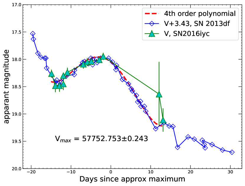
Figure B.1: Estimation of $V$-band maximum.

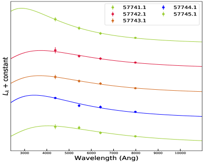
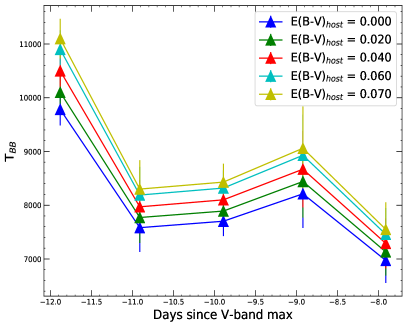
Figure B.2: Fitting black-body curves to a few early epochs of SN 2016iyc by assuming different host-galaxy extinctions. The top-left and right panels show black-body fits to a few early-epoch SEDs of SN 2016iyc corresponding to host-galaxy extinctions of 0.00 mag and 0.02 mag, respectively. The middle-left and right panels show black-body fits to a few early-epoch SEDs of SN 2016iyc corresponding to host-galaxy extinctions of 0.04 mag and 0.06 mag, respectively. The bottom-left panel shows black-body fits to a few early-epoch SEDs of SN 2016iyc corresponding to a host-galaxy extinction of 0.07 mag, while the bottom-right panel shows the variation of the black-body temperature obtained using black-body fits to the SEDs corresponding to different host-galaxy extinctions.

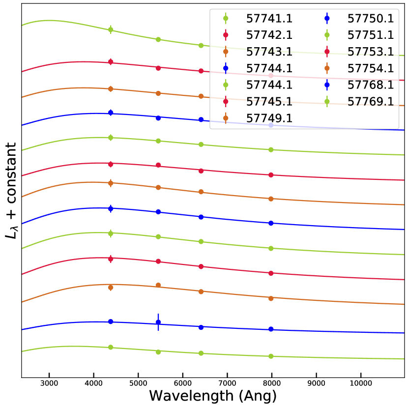
Figure B.3: The black-body fits to the SED of SN 2016iyc to estimate the bolometric light curve generated from SUPERBOL.

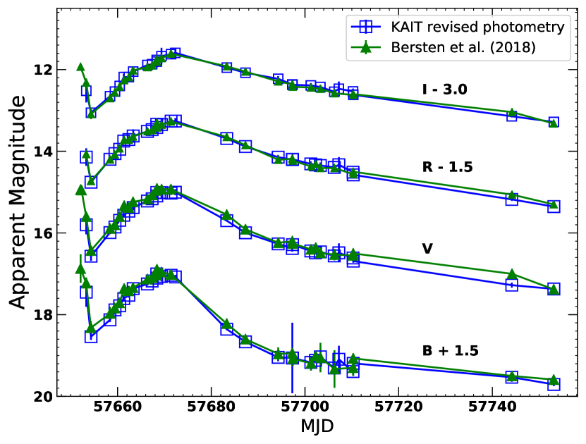
Figure B.4: Comparison between the KAIT revised photometry and the KAIT data used by Bersten et al. (2018) for SN 2016gkg.

Table B.1: MESA model and SNEC explosion parameters of SN 2011fu and SN 2016gkg.

SN name	Model Name	$M_{\rm ZAMS}$	$Z$	$f_{ov}^{a}$	$M_{\mathrm{f}}^{b}$	$M_{\mathrm{c}}^{c}$	$M_{\mathrm{ej}}^{d}$	$M_{\mathrm{Ni}}^{e}$	$E_{\mathrm{exp}}^{f}$
		(M⊙)			(M⊙)	(M⊙)	(M⊙)	(M⊙)	($10^{51}$ erg)
SN 2016gkg	He5_A	18.0	0.0200	0.01	5.00	1.6	3.40	0.087	1.30
SN 2011fu	He5_B	18.0	0.0200	0.01	5.00	1.5	3.50	0.140	1.25

^aOvershoot parameter. ^bFinal mass of the pre-SN model. ^cFinal mass of the central remnant ^dEjecta mass. ^eNickel mass ^fExplosion energy.

Table B.2: Photometry of SN 2016iyc

MJD	$B$	$V$	$R$	$C$	$I$	Telescope
	(mag)	(mag)	(mag)	(mag)	(mag)
57740.144	…	…	…	17.807 $\pm$ 0.111	…	KAIT
57741.116	18.473 $\pm$ 0.075	18.262 $\pm$ 0.074	18.081 $\pm$ 0.091	17.985 $\pm$ 0.048	17.875 $\pm$ 0.103	KAIT
57742.089	18.774 $\pm$ 0.149	18.484 $\pm$ 0.118	18.102 $\pm$ 0.147	18.057 $\pm$ 0.149	17.832 $\pm$ 0.148	KAIT
57743.109	18.875 $\pm$ 0.114	18.484 $\pm$ 0.111	18.105 $\pm$ 0.117	17.987 $\pm$ 0.135	17.949 $\pm$ 0.142	KAIT
57744.087	18.796 $\pm$ 0.139	18.451 $\pm$ 0.113	17.957 $\pm$ 0.113	17.957 $\pm$ 0.143	17.731 $\pm$ 0.126	KAIT
57744.091	18.787 $\pm$ 0.054	18.299 $\pm$ 0.050	17.933 $\pm$ 0.067	– $\pm$ –	17.656 $\pm$ 0.119	Nickel
57745.092	18.865 $\pm$ 0.129	18.237 $\pm$ 0.084	18.038 $\pm$ 0.106	17.855 $\pm$ 0.115	17.658 $\pm$ 0.114	KAIT
57749.111	18.568 $\pm$ 0.105	18.090 $\pm$ 0.081	17.728 $\pm$ 0.098	17.742 $\pm$ 0.131	17.524 $\pm$ 0.130	KAIT
57750.090	18.582 $\pm$ 0.100	18.050 $\pm$ 0.075	17.735 $\pm$ 0.080	17.693 $\pm$ 0.092	17.433 $\pm$ 0.084	KAIT
57751.095	18.567 $\pm$ 0.085	18.037 $\pm$ 0.063	17.693 $\pm$ 0.070	17.665 $\pm$ 0.055	17.439 $\pm$ 0.073	KAIT
57751.095	18.567 $\pm$ 0.085	18.037 $\pm$ 0.063	17.693 $\pm$ 0.070	17.665 $\pm$ 0.055	17.439 $\pm$ 0.073	KAIT
57753.099	18.578 $\pm$ 0.083	18.009 $\pm$ 0.061	17.679 $\pm$ 0.063	17.635 $\pm$ 0.091	17.408 $\pm$ 0.082	KAIT
57754.091	18.724 $\pm$ 0.137	17.947 $\pm$ 0.066	17.678 $\pm$ 0.067	17.653 $\pm$ 0.090	17.409 $\pm$ 0.093	KAIT
57768.107	…	18.638 $\pm$ 0.059	18.582 $\pm$ 0.395	18.570 $\pm$ 0.242	18.069 $\pm$ 0.321	KAIT
57769.105	19.295 $\pm$ 0.464	19.111 $\pm$ 0.214	18.666 $\pm$ 0.194	18.784 $\pm$ 0.282	18.466 $\pm$ 0.232	KAIT
57956.471	$>$21.490	$>$21.336	$>$21.542	…	$>$20.631	Nickel

Table B.3: Revised KAIT photometry of SN 2016gkg along with 3.6 m DOT data

MJD	$B$	$V$	$R$	$C$	$I$	Telescope
	(mag)	(mag)	(mag)	(mag)	(mag)
57653.315	15.949 $\pm$ 0.357	15.799 $\pm$ 0.234	15.642 $\pm$ 0.214	15.661 $\pm$ 0.069	15.518 $\pm$ 0.286	KAIT
57654.322	17.039 $\pm$ 0.079	16.569 $\pm$ 0.113	16.257 $\pm$ 0.053	16.272 $\pm$ 0.030	16.056 $\pm$ 0.068	KAIT
57658.373	16.626 $\pm$ 0.054	15.990 $\pm$ 0.038	15.696 $\pm$ 0.045	15.745 $\pm$ 0.045	15.652 $\pm$ 0.050	KAIT
57659.444	16.383 $\pm$ 0.049	15.854 $\pm$ 0.041	15.557 $\pm$ 0.053	15.630 $\pm$ 0.042	15.539 $\pm$ 0.063	KAIT
57660.444	16.282 $\pm$ 0.047	15.690 $\pm$ 0.018	15.450 $\pm$ 0.022	15.429 $\pm$ 0.083	15.401 $\pm$ 0.045	KAIT
57661.316	16.106 $\pm$ 0.066	15.566 $\pm$ 0.052	15.249 $\pm$ 0.061	15.482 $\pm$ 0.071	15.183 $\pm$ 0.079	KAIT
57662.408	16.024 $\pm$ 0.060	15.466 $\pm$ 0.053	15.213 $\pm$ 0.059	15.238 $\pm$ 0.062	15.182 $\pm$ 0.085	KAIT
57663.334	15.861 $\pm$ 0.074	15.378 $\pm$ 0.068	15.125 $\pm$ 0.162	15.145 $\pm$ 0.068	15.049 $\pm$ 0.109	KAIT
57666.368	15.748 $\pm$ 0.039	15.217 $\pm$ 0.034	15.013 $\pm$ 0.045	14.992 $\pm$ 0.033	14.887 $\pm$ 0.049	KAIT
57667.373	15.676 $\pm$ 0.037	15.162 $\pm$ 0.038	14.969 $\pm$ 0.051	14.931 $\pm$ 0.025	14.868 $\pm$ 0.050	KAIT
57668.362	15.504 $\pm$ 0.035	15.009 $\pm$ 0.012	14.838 $\pm$ 0.011	…	14.763 $\pm$ 0.013	KAIT
57668.375	15.605 $\pm$ 0.117	15.093 $\pm$ 0.060	14.916 $\pm$ 0.132	14.830 $\pm$ 0.084	14.805 $\pm$ 0.146	KAIT
57669.369	15.565 $\pm$ 0.117	15.011 $\pm$ 0.139	14.845 $\pm$ 0.128	14.758 $\pm$ 0.180	14.671 $\pm$ 0.024	KAIT
57671.420	15.536 $\pm$ 0.058	15.024 $\pm$ 0.043	14.760 $\pm$ 0.051	14.759 $\pm$ 0.063	14.621 $\pm$ 0.069	KAIT
57672.330	15.576 $\pm$ 0.048	15.003 $\pm$ 0.074	14.760 $\pm$ 0.072	14.723 $\pm$ 0.054	14.590 $\pm$ 0.090	KAIT
57683.307	16.856 $\pm$ 0.023	15.699 $\pm$ 0.016	15.187 $\pm$ 0.014	…	14.951 $\pm$ 0.014	KAIT
57687.298	17.165 $\pm$ 0.040	15.995 $\pm$ 0.017	15.383 $\pm$ 0.016	…	15.076 $\pm$ 0.016	KAIT
57694.279	17.545 $\pm$ 0.096	16.266 $\pm$ 0.049	15.645 $\pm$ 0.054	15.692 $\pm$ 0.053	15.226 $\pm$ 0.069	KAIT
57696.255	17.544 $\pm$ 0.021	16.302 $\pm$ 0.016	15.716 $\pm$ 0.023	…	…	3.6 m DOT
57697.300	17.560 $\pm$ 0.863	16.379 $\pm$ 0.076	15.703 $\pm$ 0.020	…	15.363 $\pm$ 0.019	KAIT
57697.350	17.562 $\pm$ 0.106	16.286 $\pm$ 0.106	15.697 $\pm$ 0.118	15.815 $\pm$ 0.016	15.372 $\pm$ 0.120	KAIT
57701.256	17.669 $\pm$ 0.081	16.440 $\pm$ 0.052	15.809 $\pm$ 0.059	15.891 $\pm$ 0.040	15.387 $\pm$ 0.059	KAIT
57702.253	17.617 $\pm$ 0.038	16.487 $\pm$ 0.018	15.833 $\pm$ 0.018	…	…	KAIT
57703.289	17.532 $\pm$ 0.108	16.463 $\pm$ 0.095	15.847 $\pm$ 0.071	15.884 $\pm$ 0.055	15.426 $\pm$ 0.053	KAIT
57706.262	17.805 $\pm$ 0.156	16.562 $\pm$ 0.071	15.894 $\pm$ 0.059	15.965 $\pm$ 0.086	15.543 $\pm$ 0.071	KAIT

Table B.4: Revised KAIT photometry of SN 2016gkg along with 3.6 m DOT data, continued…

MJD	$B$	$V$	$R$	$C$	$I$	Telescope
	(mag)	(mag)	(mag)	(mag)	(mag)
57707.237	17.592 $\pm$ 0.329	16.486 $\pm$ 0.232	15.829 $\pm$ 0.186	16.023 $\pm$ 0.037	15.469 $\pm$ 0.178	KAIT
57710.259	17.893 $\pm$ 0.085	16.612 $\pm$ 0.055	16.011 $\pm$ 0.063	16.050 $\pm$ 0.046	15.535 $\pm$ 0.070	KAIT
57710.312	16.692 $\pm$ 0.084	16.689 $\pm$ 0.038	16.077 $\pm$ 0.035	…	15.617 $\pm$ 0.021	KAIT
57744.149	18.032 $\pm$ 0.109	17.277 $\pm$ 0.061	16.678 $\pm$ 0.035	…	16.143 $\pm$ 0.027	KAIT
57753.135	18.208 $\pm$ 0.039	17.371 $\pm$ 0.089	16.854 $\pm$ 0.029	…	16.282 $\pm$ 0.026	KAIT
58080.168	22.541 $\pm$ 0.258	21.751 $\pm$ 0.225	20.821 $\pm$ 0.03	…	20.137 $\pm$ 0.055	3.6 m DOT

Appendix C Investigating the evolutions of Rotating, Population III star of 25 M_⊙ and the strength of Resulting Supernovae

C.1 Additional Figures

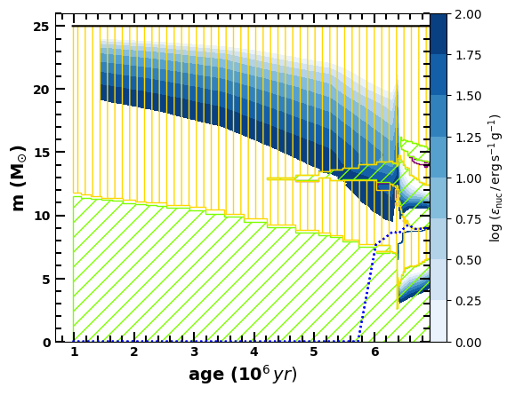
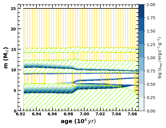
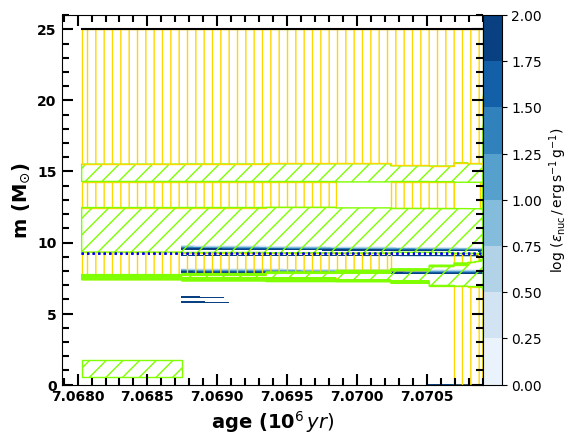
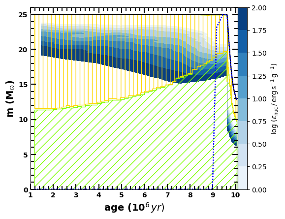
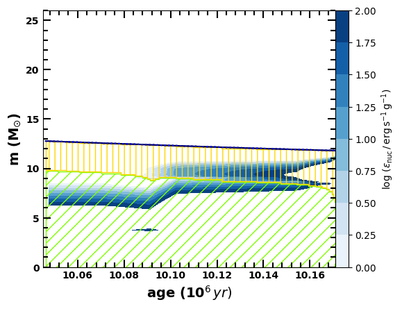
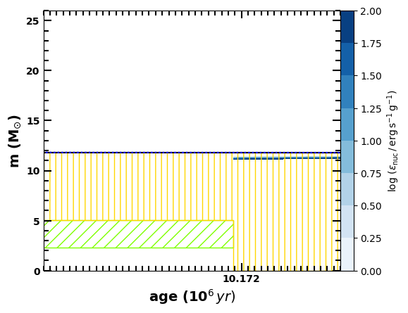
Figure C.1: The kippenhahn diagrams of the models M25_Z0.00_Rot0.2 (top) and M25_Z0.00_Rot0.8 (bottom) for a period between ZAMS to close to the pre-SN stage. Here, the green hatchings indicate the convective regions and the dark-yellow regions mark the stellar interiors where the thermohaline mixing is going on. Also, the logarithm of the specific nuclear energy generation rate ($\epsilon_{\rm nuc}$) inside the stellar interiors is indicated by the blue colour gradients. The rapidly rotating model is significantly stripped.

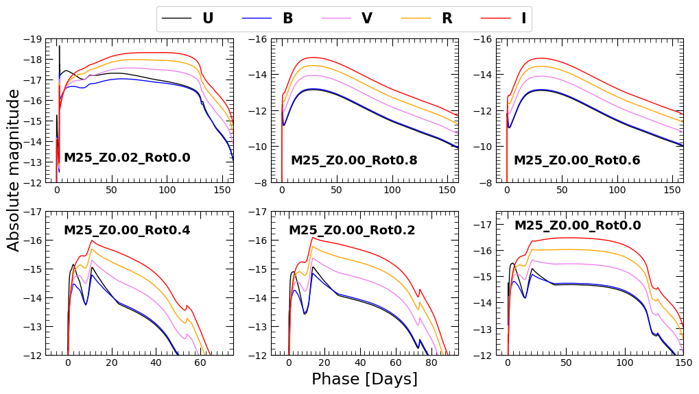
Figure C.2: The U, B, V, R, and I band light curves resulting from the synthetic explosions of Pop III models using SNEC. The non-rotating and slowly rotating models ($\Omega\,\leq\,0.4\,\Omega_{\rm crit}$) form a class of weak Type II SNe, while the rapidly rotating models ($\Omega\,\geq\,0.6\,\Omega_{\rm crit}$) result into Type Ib/c SNe within the specified limits of explosion energies and Nickel masses. The light curves resulting from the non-rotating, solar metallicity model are also shown for comparison.

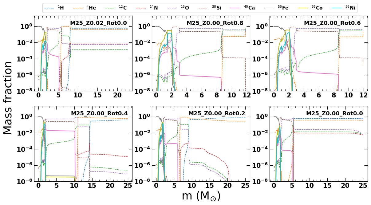
Figure C.3: A combined plot showing the mass fractions of various elements for the models in this study at a stage when the models have reached the stage of the onset of core collapse.

References

- Abbott et al. (2016) Abbott B. P., Abbott R., Abbott T. D., et al., 2016, Phys. Rev. Lett., 116, 6, 061102
- Abbott et al. (2017a) Abbott B. P., Abbott R., Abbott T. D., et al., 2017a, ApJ, 848, 2, L13
- Abbott et al. (2017b) Abbott B. P., Abbott R., Abbott T. D., et al., 2017b, Phys. Rev. Lett., 119, 16, 161101
- Abbott et al. (2020) Abbott B. P., Abbott R., Abbott T. D., et al., 2020, ApJ, 892, 1, L3
- Abbott et al. (2021a) Abbott R., Abbott T. D., Abraham S., et al., 2021a, Physical Review X, 11, 2, 021053
- Abbott et al. (2021b) Abbott R., Abbott T. D., Abraham S., et al., 2021b, ApJ, 915, 1, L5
- Abel et al. (2002) Abel T., Bryan G. L., Norman M. L., 2002, Science, 295, 5552, 93
- Abia et al. (2001) Abia C., Domínguez I., Straniero O., Limongi M., Chieffi A., Isern J., 2001, ApJ, 557, 1, 126
- Afsariardchi et al. (2021) Afsariardchi N., Drout M. R., Khatami D. K., Matzner C. D., Moon D.-S., Ni Y. Q., 2021, ApJ, 918, 2, 89
- Aldering et al. (1994) Aldering G., Humphreys R. M., Richmond M., 1994, AJ, 107, 662
- Anderson (2019) Anderson J. P., 2019, A&A, 628, A7
- Andresen et al. (2017) Andresen H., Müller B., Müller E., Janka H. T., 2017, MNRAS, 468, 2, 2032
- Ann et al. (2015) Ann H. B., Seo M., Ha D. K., 2015, ApJS, 217, 2, 27
- Arbour (2016) Arbour R., 2016, Transient Name Server Discovery Report, 2016-215, 1
- Arnett (1996) Arnett D., 1996, Supernovae and Nucleosynthesis: An Investigation of the History of Matter from the Big Bang to the Present
- Arnett (1979) Arnett W. D., 1979, ApJ, 230, L37
- Arnett (1980) Arnett W. D., 1980, ApJ, 237, 541
- Arnett (1982) Arnett W. D., 1982, ApJ, 253, 785
- Arnett & Fu (1989) Arnett W. D., Fu A., 1989, ApJ, 340, 396
- Aryan et al. (2023) Aryan A., Pandey S. B., Gupta R., Ror A. K., 2023, MNRAS, 521, 1, L17
- Aryan et al. (2022a) Aryan A., Pandey S. B., Kumar A., et al., 2022a, Journal of Astrophysics and Astronomy, 43, 2, 87
- Aryan et al. (2021a) Aryan A., Pandey S. B., Kumar A., Gupta R., Castro-Tirado A. J., Tiwari S. N., 2021a, in Revista Mexicana de Astronomia y Astrofisica Conference Series, vol. 53 of Revista Mexicana de Astronomia y Astrofisica Conference Series, 215–224
- Aryan et al. (2022b) Aryan A., Pandey S. B., Yadav A. P., Gupta R., Tiwari S. N., 2022b, Journal of Astrophysics and Astronomy, 43, 1, 2
- Aryan et al. (2021b) Aryan A., Pandey S. B., Zheng W., et al., 2021b, MNRAS, 505, 2, 2530
- Aryan et al. (2022c) Aryan A., Pandey S. B., Zheng W., et al., 2022c, MNRAS, 517, 2, 1750
- Baklanov et al. (2013) Baklanov P. V., Blinnikov S. I., Potashov M. S., Dolgov A. D., 2013, Soviet Journal of Experimental and Theoretical Physics Letters, 98, 7, 432
- Barbon et al. (1979) Barbon R., Ciatti F., Rosino L., 1979, A&A, 72, 287
- Barkana & Loeb (2001) Barkana R., Loeb A., 2001, Phys. Rep., 349, 2, 125
- Baron et al. (2000) Baron E., Branch D., Hauschildt P. H., et al., 2000, ApJ, 545, 1, 444
- Baug et al. (2018) Baug T., Ojha D. K., Ghosh S. K., et al., 2018, Journal of Astronomical Instrumentation, 7, 1, 1850003
- Baumgarte et al. (1995) Baumgarte T. W., Shapiro S. L., Teukolsky S. A., 1995, ApJ, 443, 717
- Beacom et al. (2001) Beacom J. F., Boyd R. N., Mezzacappa A., 2001, Phys. Rev. D, 63, 7, 073011
- Ben-Ami et al. (2015) Ben-Ami S., Hachinger S., Gal-Yam A., et al., 2015, ApJ, 803, 1, 40
- Bersten et al. (2011) Bersten M. C., Benvenuto O., Hamuy M., 2011, ApJ, 729, 1, 61
- Bersten et al. (2014) Bersten M. C., Benvenuto O. G., Folatelli G., et al., 2014, AJ, 148, 4, 68
- Bersten et al. (2012) Bersten M. C., Benvenuto O. G., Nomoto K., et al., 2012, ApJ, 757, 1, 31
- Bersten et al. (2016) Bersten M. C., Benvenuto O. G., Orellana M., Nomoto K., 2016, ApJ, 817, 1, L8
- Bersten et al. (2018) Bersten M. C., Folatelli G., García F., et al., 2018, Nature, 554, 7693, 497
- Bessell (1990) Bessell M. S., 1990, PASP, 102, 1181
- Blanchard et al. (2019) Blanchard P. K., Nicholl M., Berger E., et al., 2019, ApJ, 872, 1, 90
- Blinnikov et al. (2000) Blinnikov S., Lundqvist P., Bartunov O., Nomoto K., Iwamoto K., 2000, ApJ, 532, 2, 1132
- Blinnikov & Bartunov (1993) Blinnikov S. I., Bartunov O. S., 1993, A&A, 273, 106
- Blinnikov et al. (1998) Blinnikov S. I., Eastman R., Bartunov O. S., Popolitov V. A., Woosley S. E., 1998, ApJ, 496, 1, 454
- Blinnikov & Panov (1996) Blinnikov S. I., Panov I. V., 1996, Astronomy Letters, 22, 1, 39
- Blinnikov et al. (2006) Blinnikov S. I., Röpke F. K., Sorokina E. I., et al., 2006, A&A, 453, 1, 229
- Bloom et al. (1999) Bloom J. S., Kulkarni S. R., Djorgovski S. G., et al., 1999, Nature, 401, 6752, 453
- Bose et al. (2021) Bose S., Dong S., Kochanek C. S., et al., 2021, MNRAS, 503, 3, 3472
- Bostroem et al. (2019) Bostroem K. A., Valenti S., Horesh A., et al., 2019, MNRAS, 485, 4, 5120
- Brachetti et al. (1997) Brachetti P., De Felice Ciccoli M., Di Pillo G., Lucidi s., 1997, J. Glob. Optim., 10, 165
- Branch et al. (2007) Branch D., Parrent J., Troxel M. A., et al., 2007, in The Multicolored Landscape of Compact Objects and Their Explosive Origins, edited by T. di Salvo, G. L. Israel, L. Piersant, L. Burderi, G. Matt, A. Tornambe, M. T. Menna, vol. 924 of American Institute of Physics Conference Series, 342–349
- Brayton et al. (1972) Brayton R., Gustavson F., Hachtel G., 1972, Proceedings of the IEEE, 60, 1, 98
- Brecher et al. (1983) Brecher K., Fesen R. A., Maran S. P., Brandt J. C., 1983, The Observatory, 103, 106
- Bromm (2013) Bromm V., 2013, Reports on Progress in Physics, 76, 11, 112901
- Bromm et al. (1999) Bromm V., Coppi P. S., Larson R. B., 1999, ApJ, 527, 1, L5
- Brook et al. (2007) Brook C. B., Kawata D., Scannapieco E., Martel H., Gibson B. K., 2007, ApJ, 661, 1, 10
- Brown et al. (2014) Brown P. J., Breeveld A. A., Holland S., Kuin P., Pritchard T., 2014, Ap&SS, 354, 1, 89
- Bufano et al. (2014) Bufano F., Pignata G., Bersten M., et al., 2014, MNRAS, 439, 2, 1807
- Burrows & Vartanyan (2021) Burrows A., Vartanyan D., 2021, Nature, 589, 7840, 29
- Cano et al. (2017) Cano Z., Wang S.-Q., Dai Z.-G., Wu X.-F., 2017, Advances in Astronomy, 2017, 8929054
- Cao et al. (2013) Cao Y., Kasliwal M. M., Arcavi I., et al., 2013, ApJ, 775, 1, L7
- Cappellaro et al. (1999) Cappellaro E., Evans R., Turatto M., 1999, A&A, 351, 459
- Carr et al. (1984) Carr B. J., Bond J. R., Arnett W. D., 1984, ApJ, 277, 445
- Chatzopoulos & Tuminello (2019) Chatzopoulos E., Tuminello R., 2019, ApJ, 874, 1, 68
- Chatzopoulos et al. (2009) Chatzopoulos E., Wheeler J. C., Vinko J., 2009, ApJ, 704, 2, 1251