Multinomial Link Models

Abstract

We propose a unified multinomial link model for analyzing categorical responses. It not only covers the existing multinomial logistic models and their extensions as a special class, but also allows the observations with NA or Unknown responses to be incorporated as a special category in the data analysis. We provide explicit formulae for computing the likelihood gradient and Fisher information matrix, as well as detailed algorithms for finding the maximum likelihood estimates of the model parameters. Our algorithms solve the infeasibility issue of existing statistical software on estimating parameters of cumulative link models. The applications to real datasets show that the proposed multinomial link models can fit the data significantly better, and the corresponding data analysis may correct the misleading conclusions due to missing data.

Key words and phrases: Categorical data analysis, Cumulative link model, Feasible parameter space, Missing not at random, Multinomial logistic model, Partial proportional odds

1 Introduction

We consider experiments or observational studies with categorical responses, which naturally arise in many different scientific disciplines (Agresti, 2018). When the response is binary, generalized linear models have been commonly used (McCullagh and Nelder, 1989; Dobson and Barnett, 2018) to analyze the data. When responses have three or more categories, multinomial logistic models have been widely used in the literature (Glonek and McCullagh, 1995; Zocchi and Atkinson, 1999; Bu et al., 2020), which cover four kinds of logit models, baseline-category, cumulative, adjacent-categories, and continuation-ratio logit models.

Following the notations of Bu et al. (2020), there are $d$ covariates and $m\geq 2$ distinct covariate settings ${\mathbf{x}}_{i}=(x_{i1},\ldots,x_{id})^{T}$, $i=1,\ldots,m$. At the $i$th setting, $n_{i}>0$ categorical responses are collected i.i.d. from a discrete distribution with $J$ categories, which are summarized into a multinomial response ${\mathbf{Y}}_{i}=(Y_{i1},\cdots,Y_{iJ})^{T}\sim{\rm Multinomial}(n_{i};\pi_{i1},\cdots,\pi_{iJ})$, where $\pi_{ij}$ is the probability that the response falls into the $j$th category at the $i$th setting. Throughout this paper, we assume $\pi_{ij}\in(0,1)$ for all $i=1,\ldots,m$ and $j=1,\ldots,J$. The four logit models with partial proportional odds (ppo, see Lall et al. (2002); Bu et al. (2020)) can be written as follows:

$$\log\left(\frac{\pi_{ij}}{\pi_{iJ}}\right) = {\mathbf{h}}_{j}^{T}({\mathbf{x}}_{i})\boldsymbol{\beta}_{j}+{\mathbf{h}}_{c}^{T}({\mathbf{x}}_{i})\boldsymbol{\zeta}~{},\>\mbox{baseline-category}$$ (1)

$$\log\left(\frac{\pi_{i1}+\cdots+\pi_{ij}}{\pi_{i,j+1}+\cdots+\pi_{iJ}}\right) = {\mathbf{h}}_{j}^{T}({\mathbf{x}}_{i})\boldsymbol{\beta}_{j}+{\mathbf{h}}_{c}^{T}({\mathbf{x}}_{i})\boldsymbol{\zeta}~{},\>\mbox{cumulative}$$ (2)

$$\log\left(\frac{\pi_{ij}}{\pi_{i,j+1}}\right) = {\mathbf{h}}_{j}^{T}({\mathbf{x}}_{i})\boldsymbol{\beta}_{j}+{\mathbf{h}}_{c}^{T}({\mathbf{x}}_{i})\boldsymbol{\zeta}~{},\>\mbox{adjacent-categories}$$ (3)

$$\log\left(\frac{\pi_{ij}}{\pi_{i,j+1}+\cdots+\pi_{iJ}}\right) = {\mathbf{h}}_{j}^{T}({\mathbf{x}}_{i})\boldsymbol{\beta}_{j}+{\mathbf{h}}_{c}^{T}({\mathbf{x}}_{i})\boldsymbol{\zeta}~{},\>\mbox{continuation-ratio}$$ (4)

where $i=1,\ldots,m$, $j=1,\ldots,J-1$, ${\mathbf{h}}_{j}^{T}(\cdot)=(h_{j1}(\cdot),\ldots,h_{jp_{j}}(\cdot))$ are known predictor functions associated with the parameters $\boldsymbol{\beta}_{j}=(\beta_{j1},\ldots,\beta_{jp_{j}})^{T}$ for the $j$th response category, and ${\mathbf{h}}_{c}^{T}(\cdot)=(h_{1}(\cdot),\ldots,h_{p_{c}}(\cdot))$ are known predictor functions associated with the parameters $\boldsymbol{\zeta}=(\zeta_{1},\ldots,\zeta_{p_{c}})^{T}$ that are common for all categories. As special cases, ${\mathbf{h}}_{j}^{T}({\mathbf{x}}_{i})\equiv 1$ leads to proportional odds (po) models assuming the same parameters for different categories (McCullagh, 1980), and ${\mathbf{h}}_{c}^{T}({\mathbf{x}}_{i})\equiv 0$ leads to nonproportional odds (npo) models allowing all parameters to change across categories (Agresti, 2013). The corresponding expressions for po and npo models could be found in the Supplementary Materials (Sections S.7 and S.8) of Bu et al. (2020).

In the literature, the baseline-category logit model (1) is also known as the (multiclass) logistic regression model (Hastie et al., 2009), which is commonly used for nominal responses that do not have a natural ordering (Agresti, 2013). Models (2), (3), and (4) are typically used for ordinal or hierarchical responses with either a natural ordering or a hierarchical structure. According to Wang and Yang (2023), however, even for nominal responses, one can use the Akaike Information Criterion (AIC, Hirotsugu (1973); Hastie et al. (2009)) or Bayesian information criterion (BIC, Hastie et al. (2009)) to choose a working order of the response categories, treat the responses as ordinal ones, and apply models (2), (3), and (4), which may significantly improve the prediction accuracy.

The four logit models (1), (2), (3), (4) can be rewritten into a unified form (Glonek and McCullagh, 1995; Zocchi and Atkinson, 1999; Bu et al., 2020)

$${\mathbf{C}}^{T}\log({\mathbf{L}}{\bar{\boldsymbol{\pi}}}_{i})={\mathbf{X}}_{i}{\boldsymbol{\theta}},\qquad i=1,\cdots,m$$ (5)

where ${\mathbf{C}}$ is a $J\times(2J-1)$ constant matrix, ${\mathbf{L}}$ is a $(2J-1)\times J$ constant matrix depending on (1), (2), (3), and (4), $\bar{\boldsymbol{\pi}}_{i}=(\pi_{i1},\ldots,\pi_{iJ})^{T}$, ${\mathbf{X}}_{i}$ is a $J\times p$ matrix depending on ${\mathbf{h}}_{j}^{T}({\mathbf{x}}_{i})$, $j=1,\ldots,J-1$ and ${\mathbf{h}}_{c}^{T}({\mathbf{x}}_{i})$, $p=p_{1}+\cdots+p_{J-1}+p_{c}$, and $\boldsymbol{\theta}=(\boldsymbol{\beta}_{1}^{T},\ldots,\boldsymbol{\beta}_{J-1}^{T},\boldsymbol{\zeta}^{T})^{T}$.

Along another line in the literature, cumulative logit models (2) have been extended to cumulative link models or ordinal regression models (McCullagh, 1980; Agresti, 2013; Yang et al., 2017). In our notations, the cumulative link models can be written as

$$g\left(\pi_{i1}+\cdots+\pi_{ij}\right)={\mathbf{h}}_{j}^{T}({\mathbf{x}}_{i})\boldsymbol{\beta}_{j}+{\mathbf{h}}_{c}^{T}({\mathbf{x}}_{i})\boldsymbol{\zeta}$$ (6)

where the link function $g(\rho)$ could be logit, probit, log-log, complementary log-log, and cauchit (see Table 1). Note that the cumulative link model (6) with logit link is the same as the cumulative logit model (2).

Baseline-category logit model (1) has been extended with probit link, known as multinomial probit model (Aitchison and Bennett, 1970; Agresti, 2013; Greene, 2018). In our notations,

$$g\left(\frac{\pi_{ij}}{\pi_{ij}+\pi_{iJ}}\right)={\mathbf{h}}_{j}^{T}({\mathbf{x}}_{i})\boldsymbol{\beta}_{j}+{\mathbf{h}}_{c}^{T}({\mathbf{x}}_{i})\boldsymbol{\zeta}$$ (7)

where the link function $g(\rho)$ could be logit or probit. Model (7) with logit link is the same as the baseline-catetory logit model (1). Examples could be found in Agresti (2010, 2013).

Continuation-ratio logit model (4) has been extended with complementary log-log link by O’Connell (2006) for data analysis. In our notations,

$$g\left(\frac{\pi_{ij}}{\pi_{ij}+\cdots+\pi_{iJ}}\right)={\mathbf{h}}_{j}^{T}({\mathbf{x}}_{i})\boldsymbol{\beta}_{j}+{\mathbf{h}}_{c}^{T}({\mathbf{x}}_{i})\boldsymbol{\zeta}$$ (8)

where the link function $g(\rho)$ could be logit or complementary log-log. Note that model (8) with logit link is the same as the continuation-ratio logit model (4).

Given so many models have been proposed or extended for categorical responses, nevertheless, they are not flexible enough for many real applications (see Section 5). In this paper, we propose a unified categorical model, called the multinomial link model, which not only covers all the models mentioned above, but also allows more flexible model structures, mixed link functions, and response categories in multiple groups. More specifically, it allows the observations with NA or unknown responses to be incorporated as a special category and corrects misleading conclusions due to missing data.

2 Multinomial Link Models

Inspired by the unified form (5) of multinomial link models, in this section, we propose a more flexible multinomial model, called the multinomial link model, as well as its three special classes, mixed-link models allowing separate link functions for different categories, two-group models allowing multi-grouped response categories, and po-npo mixture models allowing more flexible model structures.

2.1 Multinomial link models in a unified form

In matrix form, the multinomial link model can be written as

$${\mathbf{g}}\left(\frac{{\mathbf{L}}{\boldsymbol{\pi}}_{i}}{{\mathbf{R}}\boldsymbol{\pi}_{i}+\pi_{iJ}{\mathbf{b}}}\right)={\boldsymbol{\eta}}_{i}={\mathbf{X}}_{i}{\boldsymbol{\theta}}$$ (9)

where ${\mathbf{g}}=(g_{1},\ldots,g_{J-1})^{T}$ is a vector of $J-1$ link functions, ${\mathbf{L}}$ and ${\mathbf{R}}$ are $(J-1)\times(J-1)$ constant matrices, ${\mathbf{b}}\in\mathbb{R}^{J-1}$ is a constant vector, ${\boldsymbol{\pi}}_{i}=(\pi_{i1},\ldots,\pi_{i,J-1})^{T}\in\mathbb{R}^{J-1}$, $\pi_{iJ}=1-\sum_{j=1}^{J-1}\pi_{ij}$, ${\boldsymbol{\eta}}_{i}=(\eta_{i1},\ldots,\eta_{i,J-1})^{T}\in\mathbb{R}^{J-1}$, ${\mathbf{X}}_{i}=({\mathbf{f}}_{1}({\mathbf{x}}_{i}),\ldots,{\mathbf{f}}_{J-1}({\mathbf{x}}_{i}))^{T}\in\mathbb{R}^{(J-1)\times p}$ with ${\mathbf{f}}_{j}({\mathbf{x}}_{i})=(f_{j1}({\mathbf{x}}_{i}),\ldots,f_{jp}({\mathbf{x}}_{i}))^{T}$, and the regression parameter vector $\boldsymbol{\theta}=(\theta_{1},\ldots,\theta_{p})^{T}$ consists of $p$ unknown parameters in total. Note that the vector ${\mathbf{g}}$ of link functions applies to the ratio of two vectors component-wise, which can be denoted as ${\mathbf{g}}\left(({\mathbf{L}}{\boldsymbol{\pi}}_{i})\oslash({\mathbf{R}}{\boldsymbol{\pi}}_{i}+\pi_{iJ}{\mathbf{b}})\right)$ with the notation of element-wise division “$\oslash$” (also known as Hadamard division). That is, if we denote ${\mathbf{L}}=({\mathbf{L}}_{1},\ldots,{\mathbf{L}}_{J-1})^{T}$, ${\mathbf{R}}=({\mathbf{R}}_{1},\ldots,{\mathbf{R}}_{J-1})^{T}$ and ${\mathbf{b}}=(b_{1},\ldots,b_{J-1})^{T}$, then the multinomial link model (9) can be written in its equation form

$$g_{j}\left(\frac{{\mathbf{L}}^{T}_{j}\boldsymbol{\pi}_{i}}{{\mathbf{R}}^{T}_{j}\boldsymbol{\pi}_{i}+\pi_{iJ}b_{j}}\right)=\eta_{ij}={\mathbf{f}}_{j}^{T}({\mathbf{x}}_{i})\boldsymbol{\theta},\quad j=1,\ldots,J-1$$ (10)

To simplify the notations, we define

$$\rho_{ij}=\frac{{\mathbf{L}}^{T}_{j}\boldsymbol{\pi}_{i}}{{\mathbf{R}}^{T}_{j}\boldsymbol{\pi}_{i}+\pi_{iJ}b_{j}},\quad j=1,\ldots,J-1$$ (11)

and thus $\boldsymbol{\rho}_{i}=(\rho_{i1},\ldots,\rho_{i,J-1})^{T}=\left({\mathbf{L}}{\boldsymbol{\pi}}_{i}\right)\oslash\left({\mathbf{R}}\boldsymbol{\pi}_{i}+\pi_{iJ}{\mathbf{b}}\right)$. Note that the notations of $\boldsymbol{\pi}_{i}$, $\boldsymbol{\eta}_{i}$, ${\mathbf{X}}_{i}$ are different from those in Bu et al. (2020). Special classes of the multinomial link models (9) or (10) with explicit ${\mathbf{L}}$, ${\mathbf{R}}$, and ${\mathbf{b}}$ can be found in Sections S.1 and S.2 in the Supplementary Materials.

2.2 Link functions and mixed-link models

For multinomial link models (9) or (10), we need that (i) the link functions $g_{1},\ldots,g_{J-1}$ are well defined from $\rho\in(0,1)$ to $\eta\in(-\infty,\infty)$, which are part of the model assumptions. In this paper, we also require that (ii) $g_{1}^{-1},\ldots,g_{J-1}^{-1}$ exist and are differentiable from $\eta\in(-\infty,\infty)$ to $\rho\in(0,1)$; and (iii) $g_{j}^{-1}(\eta)>0$ for all $\eta\in(-\infty,\infty)$ and $j=1,\ldots,J-1$.

In the literature, many link functions have been proposed. For examples, logit, probit, log-log, and complementary log-log links were used by McCullagh and Nelder (1989) for binary responses; cauchit link could be tracked back to Morgan and Smith (1992) for distributions with many extreme values; $t$ link was suggested first by Albert and Chib (1993) and also connected to robit regression (Liu, 2004) and Gosset link family (Koenker and Yoon, 2009); Pregibon link family (Pregibon, 1980; Koenker and Yoon, 2009; Smith et al., 2020) was introduced as a two-parameter generalization of the logit link. We skip Pregibon link in this paper since its image usually does not cover the whole real line.

In Table 1 we list possible link functions considered for multinomial link models. It should be noted that the $t$ link family $g(\rho)=F_{\nu}^{-1}(\rho)$ incorporates logit, which could be approximated by $F_{7}$ according to Liu (2004), and probit as a limit when $\nu$ goes to $\infty$. Note that $F_{\nu}$ and $f_{\nu}$ are the cumulative distribution function (cdf) and probability density function (pdf) of $t$-distribution with degrees of freedom $\nu$, respectively.

Name	$\eta=g(\rho)$	$\rho=g^{-1}(\eta)$	$\left(g^{-1}\right)^{\prime}(\eta)$
logit	$\log\left(\frac{\rho}{1-\rho}\right)$	$\frac{e^{\eta}}{1+e^{\eta}}$	$\frac{e^{\eta}}{(1+e^{\eta})^{2}}=\rho(1-\rho)$
probit	$\Phi^{-1}(\rho)$	$\Phi(\eta)$	$\phi(\eta)=\frac{1}{\sqrt{2\pi}}e^{-\frac{\eta^{2}}{2}}$
log-log	$-\log(-\log(\rho))$	$\exp\{-e^{-\eta}\}$	$\exp\{-e^{-\eta}-\eta\}=\rho e^{-\eta}$
complementary log-log	$\log(-\log(1-\rho))$	$1-\exp\{-e^{\eta}\}$	$\exp\{-e^{\eta}+\eta\}=(1-\rho)e^{\eta}$
cauchit	$\tan(\pi(\rho-1/2))$	$\frac{1}{2}+\frac{{\rm arctan}(\eta)}{\pi}$	$\frac{1}{\pi(1+\eta^{2})}$
t/robit/Gosset, $\nu>0$	$F_{\nu}^{-1}(\rho)$	$F_{\nu}(\eta)$	$f_{\nu}(\eta)=\frac{\Gamma\left(\frac{\nu+1}{2}\right)}{\sqrt{\nu\pi}\ \Gamma\left(\frac{\nu}{2}\right)}\left(1+\frac{\eta^{2}}{\nu}\right)^{-\frac{\nu+1}{2}}$

Table 1: Commonly Used Link Functions

In this section, we introduce a special class of the multinomial link models (10), which allows separate links for different categories. We will show later in Section 5.2 that a multinomial model with mixed links can fit some real data much better.

Example 2.1.

Mixed-link models with ppo Inspired by the extended models (6), (7), (8), we can extend models (1), (2), (3), and (4) by allowing mixed links to the following mixed-link models with ppo:

$$g_{j}\left(\rho_{ij}\right)={\mathbf{h}}_{j}^{T}({\mathbf{x}}_{i})\boldsymbol{\beta}_{j}+{\mathbf{h}}_{c}^{T}({\mathbf{x}}_{i})\boldsymbol{\zeta}$$ (12)

where $i=1,\ldots,m$, $j=1,\ldots,J-1$, $g_{1},\ldots,g_{J-1}$ are given link functions, and

$$\rho_{ij}=\left\{\begin{array}[]{cl}\frac{\pi_{ij}}{\pi_{ij}+\pi_{iJ}}&\mbox{, for baseline-category mixed-link model}\\ \pi_{i1}+\cdots+\pi_{ij}&\mbox{, for cumulative mixed-link model}\\ \frac{\pi_{ij}}{\pi_{ij}+\pi_{i,j+1}}&\mbox{, for adjacent-categories mixed-link model}\\ \frac{\pi_{ij}}{\pi_{ij}+\cdots+\pi_{iJ}}&\mbox{, for continuation-ratio mixed-link model}\end{array}\right.$$ (13)

The mixed-link model (12)+(13) actually covers all models mentioned in Section 1. It can also be verified that it is a special class of the multinomial link models (9) or (10) (see Section S.1 of the Supplementary Materials). $\Box$

2.3 NA category and two-group models

In practice, it is fairly common to encounter observations with NA or Unknown responses. If the missing mechanism is not at random, the analysis after removing those observations could be misleading (see, for example, Bland (2015)). Inspired by Wang and Yang (2023), one may treat NA as a special category and use AIC or BIC to choose a working order of the response categories including NA. Nevertheless, for some real applications, one working order of all response categories may not fit the data well (see Section 5.1).

In this section, we introduce a special class of the multinomial link models (9) or (10), which allows the response categories consisting of two overlapped groups, called a two-group model. One group of $k+1\geq 2$ categories are controlled by a baseline-category mixed-link model and the other group of $J-k\geq 3$ categories are controlled by a cumulative, adjacent-categories, or continuation-ratio mixed-link model. The two groups are assumed to share a same category so that all categories are connected. A special case of two-group models is that the two groups share the same baseline category $J$ (see Example S.2.1 in the Supplementary Materials). A general two-group model can be described as follows.

Example 2.2.

Two-group models with ppo In this model, we assume that the response categories consist of two groups. The first group $\{1,\ldots,k,s\}$ is controlled by a baseline-category mixed-link model with the baseline category $s$, where $1\leq k\leq J-3$ and $k+1\leq s\leq J$, while the other group $\{k+1,\ldots,J\}$ is controlled by a cumulative, adjacent-categories, or continuation-ratio mixed-link model with $J$ as the baseline category. The two groups share the category $s$ to connect all the $J$ categories. The two-group model with ppo is defined by equation (12) plus

$$\rho_{ij}=\left\{\begin{array}[]{cl}\frac{\pi_{ij}}{\pi_{ij}+\pi_{is}}&\mbox{ for }j=1,\ldots,k\\ \frac{\pi_{i,k+1}+\cdots+\pi_{ij}}{\pi_{i,k+1}+\cdots+\pi_{iJ}}&\mbox{ for baseline-cumulative and }j=k+1,\ldots,J-1\\ \frac{\pi_{ij}}{\pi_{ij}+\pi_{i,j+1}}&\mbox{ for baseline-adjacent and }j=k+1,\ldots,J-1\\ \frac{\pi_{ij}}{\pi_{ij}+\cdots+\pi_{iJ}}&\mbox{ for baseline-continuation and }j=k+1,\ldots,J-1\end{array}\right.$$ (14)

The two-group model (12)+(14) consists of three classes, baseline-cumulative, baseline-adjacent, and baseline-continuation mixed-link models with ppo, which are all special cases of the multinomial link models (9) or (10) (see Section S.2 of the Supplementary Materials for justifications and explicit expressions of ${\mathbf{L}}$, ${\mathbf{R}}$, and ${\mathbf{b}}$). $\Box$

Other structures, such as cumulative-continuation (two-group), three-group or multi-group models, can be defined similarly, which still belong to the multinomial link models.

2.4 Partially equal coefficients and po-npo mixture models

If we check the right hands of models (1), (2), (3), (4), (6), (7), (8), ppo (Lall et al., 2002; Bu et al., 2020) is currently the most flexible model structure, which allows that the parameters of some predictors are the same across different categories (the po component ${\mathbf{h}}_{c}^{T}({\mathbf{x}}_{i})\boldsymbol{\zeta}$), while the parameters of some other predictors are different across the categories (the npo component ${\mathbf{h}}_{j}^{T}({\mathbf{x}}_{i})\boldsymbol{\beta}_{j}$).

For some applications (see Section 5.3), nevertheless, it could be significantly better if we allow some (but not all) categories share the same regression coefficients of some particular predictors. For example, only the first and second categories sharing the same regression coefficients of $x_{i1}$ and $x_{i2}$, that is, follow a po model, while the third and fourth categories have their own coefficients of $x_{i1}$ and $x_{i2}$, that is, follow a npo model. The corresponding model matrix can be written as

$${\mathbf{X}}_{i}=\begin{pmatrix}1&&&&&&&&x_{i1}&x_{i2}\\ &1&&&&&&&x_{i1}&x_{i2}\\ &&1&x_{i1}&x_{i2}&&&&&\\ &&&&&1&x_{i1}&x_{i2}&&\\ \end{pmatrix}$$

with the regression parameters $\boldsymbol{\theta}=(\beta_{11},\beta_{21},\beta_{31},\beta_{32},\beta_{33},\beta_{41},\beta_{42},\beta_{43},\zeta_{1},\zeta_{2})^{T}$. Such an ${\mathbf{X}}_{i}$ does not belong to ppo models.

In this section, we introduce a special class of the multinomial link models (9) or (10), called po-npo mixture models, which allows the regression coefficients/parameters for a certain predictor to be partially equal, that is, equal across some, but not all, categories.

Example 2.3.

Po-npo mixture model We assume model (9) with the model matrix

$${\mathbf{X}}_{i}=\begin{pmatrix}{\mathbf{h}}_{1}^{T}({\mathbf{x}}_{i})&&&{\mathbf{h}}_{c1}^{T}({\mathbf{x}}_{i})\\ &\ddots&&\vdots\\ &&{\mathbf{h}}_{J-1}^{T}({\mathbf{x}}_{i})&{\mathbf{h}}_{c,J-1}^{T}({\mathbf{x}}_{i})\end{pmatrix}\>\in\mathbb{R}^{(J-1)\times p}$$ (15)

where ${\mathbf{h}}_{cj}({\mathbf{x}}_{i})=(h_{cj1}({\mathbf{x}}_{i}),\ldots,h_{cjp_{c}}({\mathbf{x}}_{i}))^{T}$ are known functions to determine the $p_{c}$ predictors associated with the $j$th category. If we write $\boldsymbol{\theta}=(\boldsymbol{\beta}_{1}^{T},\ldots,\boldsymbol{\beta}_{J-1}^{T},\boldsymbol{\zeta}^{T})^{T}$, the po-npo mixture model can be written as

$$g_{j}\left(\rho_{ij}\right)={\mathbf{h}}_{j}^{T}({\mathbf{x}}_{i})\boldsymbol{\beta}_{j}+{\mathbf{h}}_{cj}^{T}({\mathbf{x}}_{i})\boldsymbol{\zeta}$$ (16)

where $\rho_{ij}$ is given by (11).

A special case with ${\mathbf{h}}_{c1}({\mathbf{x}}_{i})=\cdots={\mathbf{h}}_{c,J-1}({\mathbf{x}}_{i})\equiv{\mathbf{h}}_{c}({\mathbf{x}}_{i})$ leads to the classical ppo model (see (S.1) in the Supplementary Materials). $\Box$

3 Parameter, Information Matrix, and Selection

3.1 Feasible parameter space

It is known that the parameter estimates $\hat{\boldsymbol{\theta}}$ found by R or SAS for cumulative logit models (2) could be infeasible. That is, $\pi_{ij}(\hat{\boldsymbol{\theta}})<0$ or $\pi_{ij}(\hat{\boldsymbol{\theta}})\notin(0,1)$ for some $i=1,\ldots,m$ and $j=1,\ldots,J$. For examples, Wang and Yang (2023) reported in their simulation studies that $44$ out of $1000$ fitted parameters by SAS PROC LOGISTIC command for cumulative logit models were not feasible.

In this section, we provide explicit formulae for $\pi_{ij}$’s as functions of parameters $\boldsymbol{\theta}$ and ${\mathbf{x}}_{i}$’s under the multinomial link models (9) or (10), and characterize the space of feasible parameters for searching parameter estimates.

Given the parameters $\boldsymbol{\theta}\in\mathbb{R}^{p}$ and a setting ${\mathbf{x}}_{i}\in\mathbb{R}^{d}$, $\eta_{ij}={\mathbf{f}}_{j}^{T}({\mathbf{x}}_{i})\boldsymbol{\theta}\in(-\infty,\infty)$ according to (10), and $\rho_{ij}=g_{j}^{-1}(\eta_{ij})\in(0,1)$ as defined in (11), $j=1,\ldots,J-1$. To generate multinomial responses under given link functions, we require $\pi_{ij}\in(0,1)$, $j=1,\ldots,J$. To solve $\boldsymbol{\pi}_{i}=(\pi_{i1},\ldots,\pi_{i,J-1})^{T}$ and $\pi_{iJ}$ from $\boldsymbol{\rho}_{i}=(\rho_{ij},\ldots,\rho_{i,J-1})^{T}$, we denote ${\mathbf{D}}_{i}={\rm diag}\left(\boldsymbol{\rho}_{i}^{-1}\right){\mathbf{L}}-{\mathbf{R}}\in\mathbb{R}^{(J-1)\times(J-1)}$, where ${\rm diag}\left(\boldsymbol{\rho}_{i}^{-1}\right)={\rm diag}\{\rho_{i1}^{-1},\ldots,\rho_{i,J-1}^{-1}\}\in\mathbb{R}^{(J-1)\times(J-1)}$. The explicit formulae are provided as follows.

Lemma 3.1.

Suppose $\rho_{ij}\in(0,1),j=1,\ldots,J-1$; ${\mathbf{D}}_{i}^{-1}$ exists; and all the $J-1$ coordinates of ${\mathbf{D}}_{i}^{-1}{\mathbf{b}}$ are positive. Then model (9) implies a unique $\boldsymbol{\pi}_{i}$ as a function of $\boldsymbol{\rho}_{i}$:

$$\boldsymbol{\pi}_{i}=\frac{{\mathbf{D}}_{i}^{-1}{\mathbf{b}}}{1+{\mathbf{1}}^{T}_{J-1}{\mathbf{D}}_{i}^{-1}{\mathbf{b}}}$$ (17)

as well as $\pi_{iJ}=\left(1+{\mathbf{1}}^{T}_{J-1}{\mathbf{D}}_{i}^{-1}{\mathbf{b}}\right)^{-1}$ such that $\boldsymbol{\pi}_{ij}\in(0,1)$ for all $j=1,\ldots,J$, where ${\mathbf{1}}_{J-1}$ is a vector consisting of $J-1$ ones.

The proof of Lemma 3.1, as well as other proofs, is relegated to Section S.5 of the Supplementary Materials.

According to Lemma 3.1, it is sufficient for $\pi_{ij}\in(0,1)$ to let ${\mathbf{D}}_{i}^{-1}$ exist and all the $J-1$ coordinates of ${\mathbf{D}}_{i}^{-1}{\mathbf{b}}$ to be positive. Given the data with the observed set of distinct settings $\{{\mathbf{x}}_{1},\ldots,{\mathbf{x}}_{m}\}$, we define the feasible parameter space of model (9) or (10) as

$$\boldsymbol{\Theta}=\left\{\boldsymbol{\theta}\in\mathbb{R}^{p}\mid{\mathbf{D}}_{i}^{-1}\mbox{ exists, all coordinates of }{\mathbf{D}}_{i}^{-1}{\mathbf{b}}\mbox{ are positive},i=1,\ldots,m\right\}$$ (18)

Note that $\boldsymbol{\Theta}$ itself is either $\mathbb{R}^{p}$ or an open subset of $\mathbb{R}^{p}$. Nevertheless, for typical applications, we may use a bounded subset of $\boldsymbol{\Theta}$, which is expected to cover the true $\boldsymbol{\theta}$ as an interior point, as the working parameter space to achieve desired theoretical properties.

Theorem 3.1.

Consider the mixed-link models (12)+(13) with the observed set of distinct settings $\{{\mathbf{x}}_{1},\ldots,{\mathbf{x}}_{m}\}$ and parameters $\boldsymbol{\theta}=(\boldsymbol{\beta}_{1}^{T},\ldots,\boldsymbol{\beta}_{J-1}^{T},\boldsymbol{\zeta}^{T})^{T}\in\mathbb{R}^{p}$.

• For baseline-category, adjacent-categories, and continuation-ratio mixed-link models, the feasible parameter space $\boldsymbol{\Theta}=\mathbb{R}^{p}$.

• For cumulative mixed-link models, $\boldsymbol{\Theta}=\{\boldsymbol{\theta}\in\mathbb{R}^{p}\mid\rho_{i1}<\cdots<\rho_{i,J-1},i=1,\ldots,m\}$, where $\rho_{ij}=g_{j}^{-1}({\mathbf{h}}_{j}^{T}({\mathbf{x}}_{i})\boldsymbol{\beta}_{j}+{\mathbf{h}}_{cj}^{T}({\mathbf{x}}_{i})\boldsymbol{\zeta})$.

• For cumulative mixed-link models, if $g_{1}=\cdots=g_{J-1}=g$ and $g$ is strictly increasing, then $\boldsymbol{\Theta}=\{\boldsymbol{\theta}\in\mathbb{R}^{p}\mid{\mathbf{h}}_{j}^{T}({\mathbf{x}}_{i})\boldsymbol{\beta}_{j}<{\mathbf{h}}_{j+1}^{T}({\mathbf{x}}_{i})\boldsymbol{\beta}_{j+1},j=1,\ldots,J-2,i=1,\ldots,m\}$.

$\Box$

Theorem 3.1 shows that the feasible parameter space defined in (18) for the multinomial link models (9) or (10) is consistent with the one for the classical cumulative link models (6), which require all $\pi_{ij}\in(0,1)$. Note that if $g$ is strictly decreasing in Theorem 3.1(iii), then $\boldsymbol{\Theta}=\{\boldsymbol{\theta}\in\mathbb{R}^{p}\mid{\mathbf{h}}_{j}^{T}({\mathbf{x}}_{i})\boldsymbol{\beta}_{j}>{\mathbf{h}}_{j+1}^{T}({\mathbf{x}}_{i})\boldsymbol{\beta}_{j+1},j=1,\ldots,J-2,i=1,\ldots,m\}$.

For general multinomial link models especially with a cumulative component involved, for example, in a two-group model (12)+(14), one can always use (18) to validate the feasibility of $\boldsymbol{\theta}$.

3.2 Fisher information matrix

There are many reasons that we need to calculate the Fisher information matrix ${\mathbf{F}}(\boldsymbol{\theta})$, for examples, when finding the maximum likelihood estimate (MLE) $\hat{\boldsymbol{\theta}}$ of $\boldsymbol{\theta}$ using the Fisher scoring method (see Section 4.1), constructing confidence intervals of $\boldsymbol{\theta}$ (see Section 3.4), or finding optimal designs (Atkinson et al., 2007; Bu et al., 2020). Inspired by Theorem 2.1 in Bu et al. (2020) for multinomial logistic models (5), in this section, we provide explicit formulae for calculating ${\mathbf{F}}(\boldsymbol{\theta})$, $\boldsymbol{\theta}\in\boldsymbol{\Theta}$ for general multinomial link models (9) or (10).

Suppose for distinct ${\mathbf{x}}_{i},i=1,\cdots,m$, we have independent multinomial responses ${\mathbf{Y}}_{i}=(Y_{i1},\cdots,Y_{iJ})^{T}\sim{\rm Multinomial}(n_{i};\pi_{i1},\cdots,\pi_{iJ})$, where $n_{i}=\sum_{j=1}^{J}Y_{ij}$. Then the log-likelihood for the multinomial model is

$$l(\boldsymbol{\theta})=\log\prod_{i=1}^{m}\frac{{n_{i}}!}{{Y_{i1}}!\cdots{Y_{iJ}}!}\pi_{i1}^{Y_{i1}}\cdots\pi_{iJ}^{Y_{iJ}}=\sum_{i=1}^{m}{\mathbf{Y}}_{i}^{T}\log\bar{\boldsymbol{\pi}}_{i}+\sum_{i=1}^{m}\log(n_{i}!)-\sum_{i=1}^{m}\sum_{j=1}^{J}\log(Y_{ij}!)$$

where $\bar{\boldsymbol{\pi}}_{i}=(\pi_{i1},\ldots,\pi_{iJ})^{T}=(\boldsymbol{\pi}_{i}^{T},\pi_{iJ})^{T}$, $\log\bar{\boldsymbol{\pi}}_{i}=(\log\pi_{i1},\cdots,\log\pi_{iJ})^{T}$.

Using matrix differentiation formulae (see, for example, Seber (2008, Chapter 17)), we obtain the score vector $\partial l/\partial\boldsymbol{\theta}^{T}$ and the Fisher information matrix for general model (9) as follows (please see Section S.3 of the Supplementary Materials for more details).

Theorem 3.2.

Consider the multinomial link model (9) with distinct settings ${\mathbf{x}}_{1},\ldots,{\mathbf{x}}_{m}$ and independent response observations. Suppose $\boldsymbol{\theta}\in\boldsymbol{\Theta}$. Then the score vector

$$\frac{\partial l}{\partial\boldsymbol{\theta}^{T}}=\sum_{i=1}^{m}{\mathbf{Y}}_{i}^{T}{\rm diag}(\bar{\boldsymbol{\pi}}_{i})^{-1}\frac{\partial\bar{\boldsymbol{\pi}}_{i}}{\partial\boldsymbol{\theta}^{T}}$$ (19)

satisfying $E(\partial l/\partial\boldsymbol{\theta}^{T})=0$, and the Fisher information matrix

$${\mathbf{F}}=\sum_{i=1}^{m}n_{i}{\mathbf{F}}_{i}$$ (20)

where

$${\mathbf{F}}_{i} = \left(\frac{\partial\bar{\boldsymbol{\pi}}_{i}}{\partial\boldsymbol{\theta}^{T}}\right)^{T}{\rm diag}(\bar{\boldsymbol{\pi}}_{i})^{-1}\frac{\partial\bar{\boldsymbol{\pi}}_{i}}{\partial\boldsymbol{\theta}^{T}}$$ (21)

$$\frac{\partial\bar{\boldsymbol{\pi}}_{i}}{\partial\boldsymbol{\theta}^{T}} = {\mathbf{E}}_{i}{\mathbf{D}}_{i}^{-1}\cdot{\rm diag}\left({\mathbf{L}}\boldsymbol{\pi}_{i}\right)\cdot{\rm diag}\left(\boldsymbol{\rho}_{i}^{-2}\right)\cdot{\rm diag}\left(\left({\mathbf{g}}^{-1}\right)^{\prime}\left(\boldsymbol{\eta}_{i}\right)\right)\cdot{\mathbf{X}}_{i}$$ (22)

$${\mathbf{E}}_{i} = \left[\begin{array}[]{c}I_{J-1}\\ {\mathbf{0}}_{J-1}^{T}\end{array}\right]-\bar{\boldsymbol{\pi}}_{i}{\mathbf{1}_{J-1}^{T}}\quad\in\mathbb{R}^{J\times(J-1)}$$ (25)

${\rm diag}(\left({\mathbf{g}}^{-1}\right)^{\prime}\left(\boldsymbol{\eta}_{i}\right))={\rm diag}\{\left(g_{1}^{-1}\right)^{\prime}\left(\eta_{i1}\right),\ldots,\left(g_{J-1}^{-1}\right)^{\prime}\left(\eta_{i,J-1}\right)\}\in\mathbb{R}^{(J-1)\times(J-1)}$, $I_{J-1}$ is the identity matrix of order $J-1$, ${\mathbf{0}}_{J-1}$ is a vector of zeros in $\mathbb{R}^{J-1}$, and ${\mathbf{1}}_{J-1}$ is a vector of ones in $\mathbb{R}^{J-1}$. $\Box$

Theorem 3.2 covers the conclusion of Theorem 2.1 in Bu et al. (2020) as a special case.

3.3 Positive definiteness of Fisher information matrix

In this section, we explore when the Fisher information matrix ${\mathbf{F}}$ is positive definite, which is critical not only for the existence of ${\mathbf{F}}^{-1}$, but also for the existence of unbiased estimates of a feasible parameter $\boldsymbol{\theta}$ with finite variance (Stoica and Marzetta, 2001) and relevant optimal design problems (Bu et al., 2020).

To investigate the rank of ${\mathbf{F}}$, we denote a $J\times(J-1)$ matrix

$${\mathbf{C}}_{i}\stackrel{{\scriptstyle\triangle}}{{=}}\left({\mathbf{c}}_{i1},\ldots,{\mathbf{c}}_{i,J-1}\right)={\mathbf{E}}_{i}{\mathbf{D}}_{i}^{-1}\cdot{\rm diag}\left({\mathbf{L}}\boldsymbol{\pi}_{i}\right)\cdot{\rm diag}\left(\boldsymbol{\rho}_{i}^{-2}\right)\cdot{\rm diag}\left(\left({\mathbf{g}}^{-1}\right)^{\prime}\left(\boldsymbol{\eta}_{i}\right)\right)$$ (26)

where ${\mathbf{c}}_{i1},\ldots,{\mathbf{c}}_{i,J-1}\in\mathbb{R}^{J}$ are its column vectors. Then $\partial\bar{\boldsymbol{\pi}}_{i}/\partial\boldsymbol{\theta}^{T}={\mathbf{C}}_{i}{\mathbf{X}}_{i}$ according to (22). We further denote a $(J-1)\times(J-1)$ matrix ${\mathbf{U}}_{i}\stackrel{{\scriptstyle\triangle}}{{=}}\left(u_{st}(\boldsymbol{\pi}_{i})\right)_{s,t=1,\ldots,J-1}={\mathbf{C}}_{i}^{T}{\rm diag}(\bar{\boldsymbol{\pi}}_{i})^{-1}{\mathbf{C}}_{i}$ whose $(s,t)$th entry $u_{st}(\boldsymbol{\pi}_{i})={\mathbf{c}}_{is}^{T}{\rm diag}(\bar{\boldsymbol{\pi}}_{i})^{-1}{\mathbf{c}}_{it}$ . Then ${\mathbf{F}}_{i}={\mathbf{X}}_{i}^{T}{\mathbf{U}}_{i}{\mathbf{X}}_{i}$ according to Theorem 3.2.

Lemma 3.2.

Suppose $\boldsymbol{\theta}\in\boldsymbol{\Theta}$. Then ${\rm rank}({\mathbf{U}}_{i})=J-1$ and ${\rm rank}({\mathbf{F}}_{i})={\rm rank}({\mathbf{X}}_{i})$. $\Box$

We further define an $m(J-1)\times m(J-1)$ matrix ${\mathbf{U}}=({\mathbf{U}}_{st})_{s,t=1,\ldots,J-1}$ with ${\mathbf{U}}_{st}={\rm diag}\{n_{1}u_{st}({\boldsymbol{\pi}}_{1}),\ldots,n_{m}u_{st}({\boldsymbol{\pi}}_{m})\}$. Recall that the model matrix for general multinomial link models (9) is

$${\mathbf{X}}_{i}=({\mathbf{f}}_{1}({\mathbf{x}}_{i}),\ldots,{\mathbf{f}}_{J-1}({\mathbf{x}}_{i}))^{T}=(f_{jl}({\mathbf{x}}_{i}))_{j=1,\ldots,J-1;l=1,\ldots,p}$$ (27)

To explore the positive definiteness of ${\mathbf{F}}$, we define a $p\times m(J-1)$ matrix

$${\mathbf{H}}=({\mathbf{f}}_{1}({\mathbf{x}}_{1}),\ldots,{\mathbf{f}}_{1}({\mathbf{x}}_{m}),\ldots,{\mathbf{f}}_{J-1}({\mathbf{x}}_{1}),\ldots,{\mathbf{f}}_{J-1}({\mathbf{x}}_{m}))=\left[\begin{array}[]{ccc}{\mathbf{F}}_{11}^{T}&\cdots&{\mathbf{F}}_{J-1,1}^{T}\\ \vdots&\cdots&\vdots\\ {\mathbf{F}}_{1p}^{T}&\cdots&{\mathbf{F}}_{J-1,p}^{T}\end{array}\right]$$ (28)

where ${\mathbf{F}}_{jl}=(f_{jl}({\mathbf{x}}_{1}),\ldots,f_{jl}({\mathbf{x}}_{m}))^{T}\in\mathbb{R}^{m}$.

Example 3.1.

General ppo model For ppo models including Examples 2.1 and 2.2

$${\mathbf{H}}=\left(\begin{array}[]{ccc}{\mathbf{H}}_{1}&&\\ &\ddots&\\ &&{\mathbf{H}}_{J-1}\\ {\mathbf{H}}_{c}&\cdots&{\mathbf{H}}_{c}\end{array}\right)\>\in\>\mathbb{R}^{p\times m(J-1)}$$

where ${\mathbf{H}}_{j}=({\mathbf{h}}_{j}({\mathbf{x}}_{1}),\cdots,{\mathbf{h}}_{j}({\mathbf{x}}_{m}))\in\mathbb{R}^{p_{j}\times m}$, and ${\mathbf{H}}_{c}=({\mathbf{h}}_{c}({\mathbf{x}}_{1}),\cdots,{\mathbf{h}}_{c}({\mathbf{x}}_{m}))\in\mathbb{R}^{p_{c}\times m}$. $\Box$

Example 2.3 (continued) For po-npo mixture models,

$${\mathbf{H}}=\left(\begin{array}[]{ccc}{\mathbf{H}}_{1}&&\\ &\ddots&\\ &&{\mathbf{H}}_{J-1}\\ {\mathbf{H}}_{c1}&\cdots&{\mathbf{H}}_{c,J-1}\end{array}\right)\>\in\>\mathbb{R}^{p\times m(J-1)}$$

where ${\mathbf{H}}_{j}=({\mathbf{h}}_{j}({\mathbf{x}}_{1}),\ldots,{\mathbf{h}}_{j}({\mathbf{x}}_{m}))\in\mathbb{R}^{p_{j}\times m}$, and ${\mathbf{H}}_{cj}=({\mathbf{h}}_{cj}({\mathbf{x}}_{1}),\ldots,{\mathbf{h}}_{cj}({\mathbf{x}}_{m}))\in\mathbb{R}^{p_{c}\times m}$. $\Box$

Theorem 3.3.

For the multinomial link model (9) with $n_{i}>0$ independent observations at distinct setting ${\mathbf{x}}_{i}$, $i=1,\ldots,m$, its Fisher information matrix ${\mathbf{F}}={\mathbf{H}}{\mathbf{U}}{\mathbf{H}}^{T}$. Since $\left(g_{j}^{-1}\right)^{\prime}(\eta_{ij})\neq 0$ for all $i=1,\ldots,m$ and $j=1,\ldots,J-1$, then ${\mathbf{F}}$ at a feasible parameter $\boldsymbol{\theta}$ is positive definite if and only if ${\mathbf{H}}$ is of full row rank.

According to Theorem 3.3, the positive definiteness of ${\mathbf{F}}$ at a feasible $\boldsymbol{\theta}$ depends only on the predictor functions and the distinct settings ${\mathbf{x}}_{1},\ldots,{\mathbf{x}}_{m}$. From a design point of view, one needs to collect observations from a large enough set $\{{\mathbf{x}}_{1},\ldots,{\mathbf{x}}_{m}\}$ of distinct experiments settings. From a data analysis point of view, given the data with the set $\{{\mathbf{x}}_{1},\ldots,{\mathbf{x}}_{m}\}$ of distinct settings, there is a limit of model complexity beyond which not all parameters are estimable.

3.4 Confidence intervals and hypothesis tests for $\boldsymbol{\theta}$

In this paper, we use maximum likelihood for estimating $\boldsymbol{\theta}$. That is, we look for $\hat{\boldsymbol{\theta}}$ which maximizes the likelihood function $L(\boldsymbol{\theta})$ or the log-likelihood function $l(\boldsymbol{\theta})$, known as the maximum likelihood estimate (MLE, see, for example, Section 1.3.1 in Agresti (2013) for justifications on adopting MLE).

Under regularity conditions (see, for example, Section 5f in Rao (1973) or Chapter 18 in Ferguson (1996)), asymptotically we have $\hat{\boldsymbol{\theta}}$ is unbiased, normally distributed with ${\rm Cov}(\hat{\boldsymbol{\theta}})={\mathbf{F}}(\boldsymbol{\theta})^{-1}$. Denoting ${\mathbf{F}}(\hat{\boldsymbol{\theta}})^{-1}=\left(\hat{\sigma}_{ij}\right)_{i,j=1,\ldots,p}$, we construct approximate confidence intervals $\theta_{i}\in(\hat{\theta}_{i}-z_{\alpha/2}\sqrt{\hat{\sigma}_{ii}},\ \hat{\theta}_{i}+z_{\alpha/2}\sqrt{\hat{\sigma}_{ii}})$ with $\boldsymbol{\theta}=(\theta_{1},\ldots,\theta_{p})^{T}$ and $\hat{\boldsymbol{\theta}}=(\hat{\theta}_{1},\ldots,\hat{\theta}_{p})^{T}$, where $z_{\alpha/2}$ is the upper $(\alpha/2)$th quantile of $N(0,1)$.

To test $H_{0}:\boldsymbol{\theta}=\boldsymbol{\theta}_{0}$, we may use Wald statistic (Wald, 1943; Agresti, 2013), which asymptotically is $W=(\hat{\boldsymbol{\theta}}-\boldsymbol{\theta}_{0})^{T}{\mathbf{F}}(\hat{\boldsymbol{\theta}})(\hat{\boldsymbol{\theta}}-\boldsymbol{\theta}_{0})\stackrel{{\scriptstyle H_{0}}}{{\sim}}\chi^{2}_{p}$ .

Suppose $\boldsymbol{\theta}=(\boldsymbol{\theta}_{0}^{T},\boldsymbol{\theta}_{1}^{T})^{T}$ with $\boldsymbol{\theta}_{0}\in\mathbb{R}^{r}$ and $\boldsymbol{\theta}_{1}\in\mathbb{R}^{p-r}$. To test $H_{0}:\boldsymbol{\theta}_{0}={\mathbf{0}}$, we may use the likelihood-ratio test (Wilks, 1935, 1938; Agresti, 2013)

$$\Lambda=-2\log\frac{\max_{\boldsymbol{\theta}_{1}}L(\boldsymbol{\theta}_{1})}{\max_{\boldsymbol{\theta}}L(\boldsymbol{\theta})}\stackrel{{\scriptstyle H_{0}}}{{\sim}}\chi^{2}_{r}$$

asymptotically, which can be used before removing more than one predictors simultaneously for variable selection purposes.

3.5 Model selection

Given data $({\mathbf{x}}_{i},{\mathbf{y}}_{i}),i=1,\cdots,m$, where ${\mathbf{y}}_{i}=(y_{i1},\cdots,y_{iJ})^{T}$ satisfying $n_{i}=\sum_{j=1}^{J}y_{ij}$. Suppose the MLE $\hat{\boldsymbol{\theta}}\in\mathbb{R}^{p}$ has been obtained. Following Lemma 3.1, we obtain $\hat{\pi}_{ij}=\pi_{ij}(\hat{\boldsymbol{\theta}})$, $i=1,\ldots,m$, $j=1,\ldots,J$. Then the maximized log-likelihood

$$l(\hat{\boldsymbol{\theta}})=\sum_{i=1}^{m}\log(n_{i}!)+\sum_{i=1}^{m}{\mathbf{y}}_{i}^{T}\log\hat{\bar{\boldsymbol{\pi}}}_{i}-\sum_{i=1}^{m}\sum_{j=1}^{J}\log(y_{ij}!)$$

where $\log\hat{\bar{\boldsymbol{\pi}}}_{i}=(\log\hat{\pi}_{i1},\cdots,\log\hat{\pi}_{iJ})^{T}$. We may use AIC or BIC to choose the most appropriate model (see, for example, Hastie et al. (2009), for a good review). More specifically,

$${\rm AIC} = -\frac{2}{n}\cdot l(\hat{\boldsymbol{\theta}})+2\cdot\frac{p}{n}$$

$${\rm BIC} = -2\cdot l(\hat{\boldsymbol{\theta}})+(\log n)\cdot p$$

where $n=\sum_{i=1}^{m}n_{i}$. Note that a smaller AIC or BIC value indicates a better model.

4 Formulae and Algorithms

For facilitate the readers, we provide a summary of notations for specifying a multinomial link model in Section S.4 of the Supplementary Materials. In this section, we provide detailed formulae and algorithms for finding the MLE of $\boldsymbol{\theta}$ for a general multinomial link model (9) or (10), given a dataset in its summarized form $\{({\mathbf{x}}_{i},{\mathbf{y}}_{i})\mid i=1,\ldots,m\}$, where ${\mathbf{x}}_{i}\in\mathbb{R}^{d},i=1,\ldots,m$ are distinct settings, ${\mathbf{y}}_{i}=(y_{i1},\ldots,y_{iJ})^{T},i=1,\ldots,m$ are vectors of nonnegative integers with $\sum_{j=1}^{J}y_{ij}=n_{i}>0$, $i=1,\ldots,m$. We also provide a backward selection algorithm for finding the most appropriate po-npo mixture model.

4.1 Fisher scoring method for estimating $\boldsymbol{\theta}$

For numerically finding the MLE $\hat{\boldsymbol{\theta}}$, we adopt the Fisher scoring method described, for example, in Osborne (1992) or Chapter 14 in Lange (2010). That is, if we have $\boldsymbol{\theta}^{(t)}$ at the $t$th iteration, we obtain

$$\boldsymbol{\theta}^{(t+1)}=\boldsymbol{\theta}^{(t)}+\delta\left({\mathbf{F}}(\boldsymbol{\theta}^{(t)})\right)^{-1}\frac{\partial l}{\partial\boldsymbol{\theta}^{T}}(\boldsymbol{\theta}^{(t)})$$

at the $(t+1)$th iteration, where $\delta\in(0,1]$ is a step length which is chosen to let $l({\boldsymbol{\theta}}^{(t+1)})>l({\boldsymbol{\theta}}^{(t)})$ and $\pi_{ij}(\boldsymbol{\theta}^{(t+1)})\in(0,1)$ for all $i=1,\ldots,m$ and $j=1,\ldots,J$, ${\mathbf{F}}(\boldsymbol{\theta}^{(t)})$ is the Fisher information matrix at $\boldsymbol{\theta}=\boldsymbol{\theta}^{(t)}$, and $\frac{\partial l}{\partial\boldsymbol{\theta}^{T}}(\boldsymbol{\theta}^{(t)})$ is expression (19) evaluated at $\boldsymbol{\theta}=\boldsymbol{\theta}^{(t)}$. Theoretical justifications and more discussions on the Fisher scoring method could be found in Osborne (1992), Lange (2010), and references therein.

Algorithm 1.

Fisher scoring algorithm for finding $\hat{\boldsymbol{\theta}}$

• Input: Data ${\mathbf{x}}_{i}=(x_{i1},\ldots,x_{id})^{T},{\mathbf{y}}_{i}=(y_{i1},\ldots,y_{iJ})^{T}$, $i=1,\ldots,m$; the tolerance level of relative error $\epsilon>0$ (e.g., $\epsilon=1\times 10^{-6}$); and the step length $\delta\in(0,1)$ of linear search (e.g., $\delta=0.5$).

• Obtain an initial parameter estimate ${\boldsymbol{\theta}}^{(0)}\in\boldsymbol{\Theta}\subseteq\mathbb{R}^{p}$ (see Algorithms 2 and 3).

• Given ${\boldsymbol{\theta}}^{(t)}$, calculate the gradient $\left.\frac{\partial l}{\partial\boldsymbol{\theta}}\right|_{\boldsymbol{\theta}={\boldsymbol{\theta}}^{(t)}}$ and the Fisher information matrix ${\mathbf{F}}({\boldsymbol{\theta}}^{(t)})$ (see Algorithm 4).

• Set the initial power index $s=0$ for step length; calculate the maximum change

  $$\Delta\boldsymbol{\theta}={\mathbf{F}}(\boldsymbol{\theta}^{(t)})^{-1}\left.\frac{\partial l}{\partial\boldsymbol{\theta}^{T}}\right|_{\boldsymbol{\theta}=\boldsymbol{\theta}^{(t)}}$$

  and its Euclidean length $\|\Delta\boldsymbol{\theta}\|$.

• Calculate the parameter estimate candidate $\boldsymbol{\theta}^{*}={\boldsymbol{\theta}}^{(t)}+\delta^{s}\cdot\Delta\boldsymbol{\theta}$.

• If $\frac{\delta^{s}\|\Delta\boldsymbol{\theta}\|}{\max\{1,\|{\boldsymbol{\theta}}^{(t)}\|\}}<\epsilon$, go to Step $7^{\circ}$;
  else if $\boldsymbol{\theta}^{*}\notin\boldsymbol{\Theta}$, then replace $s$ with $s+1$ and go back to Step $4^{\circ}$;
  else if $\frac{l(\boldsymbol{\theta}^{*})-l(\boldsymbol{\theta}^{(t)})}{\max\{1,|l(\boldsymbol{\theta}^{(t)})|\}}<\epsilon$, then replace $s$ with $s+1$ and go back to Step $4^{\circ}$.

• Let $\boldsymbol{\theta}^{(t+1)}=\boldsymbol{\theta}^{*}$, replace $t$ with $t+1$, and go back to Step $2^{\circ}$.

• Output $\hat{\boldsymbol{\theta}}=\boldsymbol{\theta}^{(t)}$ as the maximum likelihood estimate of $\boldsymbol{\theta}$.

It can be verified that Algorithm 1 is valid. First of all, according to, for example, Section 14.3 of Lange (2010), $l(\boldsymbol{\theta}^{*})>l(\boldsymbol{\theta}^{(t)})$ for large enough $s$ or small enough $\delta^{s}$ if ${\mathbf{F}}(\boldsymbol{\theta}^{(t)})$ is positive definite. Secondly, since $\boldsymbol{\Theta}$ is open (see Section 3.1), $\boldsymbol{\theta}^{(t)}\in\boldsymbol{\Theta}$ must be an interior point, then $\boldsymbol{\theta}^{*}\in\boldsymbol{\Theta}$ for large enough $s$.

It should also be noted that it could be tricky to calculate ${\mathbf{F}}(\boldsymbol{\theta}^{(t)})^{-1}$ numerically while keeping its positive definiteness, especially when some eigenvalues of ${\mathbf{F}}(\boldsymbol{\theta}^{(t)})$ are tiny, which should be continuously monitored.

4.2 Finding initial parameter values

Step $1^{\circ}$ of Algorithm 1 is critical and nontrivial for multinomial link models when a cumulative component involved. In this section we first provide Algorithm 2 for finding a possible initial estimate $\boldsymbol{\theta}^{(0)}$ of $\boldsymbol{\theta}$, which is expected not far away from the MLE $\hat{\boldsymbol{\theta}}$. One needs to use (18) to check whether the $\boldsymbol{\theta}^{(0)}$ obtained by Algorithm 2 is feasible. If not, we provide Algorithm 3 to pull $\boldsymbol{\theta}^{(0)}$ back to the feasible domain $\boldsymbol{\Theta}$.

Algorithm 2.

Finding an initial estimate of $\boldsymbol{\theta}$ for model (9) or (10)

• Input: ${\mathbf{x}}_{i}=(x_{i1},\ldots,x_{id})^{T},{\mathbf{y}}_{i}=(y_{i1},\ldots,y_{iJ})^{T}$, $i=1,\ldots,m$.

• Calculate $n_{i}=\sum_{j=1}^{J}y_{ij}>0$ and $\pi_{ij}^{(0)}=\frac{y_{ij}+1}{n_{i}+J}$, $j=1,\ldots,J$, and denote $\boldsymbol{\pi}_{i}^{(0)}=(\pi_{i1}^{(0)},\ldots,\pi_{i,J-1}^{(0)})^{T}\in\mathbb{R}^{J-1}$, $i=1,\ldots,m$.

• Calculate $\rho_{ij}^{(0)}=\frac{{\mathbf{L}}_{j}^{T}{\boldsymbol{\pi}}_{i}^{(0)}}{{\mathbf{R}}_{j}^{T}\boldsymbol{\pi}_{i}^{(0)}+\pi_{iJ}^{(0)}b_{j}},j=1,\ldots,J-1$ and denote $\boldsymbol{\rho}_{i}^{(0)}=(\rho_{i1}^{(0)},\ldots,\rho_{i,J-1}^{(0)})^{T}$, $i=1,\ldots,m$.

• Calculate $\eta_{ij}^{(0)}=g_{j}(\rho_{ij}^{(0)})$, $j=1,\ldots,J-1$ and denote $\boldsymbol{\eta}_{i}^{(0)}=(\eta_{i1}^{(0)},\ldots,\eta_{i,J-1}^{(0)})^{T}\in\mathbb{R}^{J-1}$, $i=1,\ldots,m$.

• Calculate ${\mathbf{X}}_{i},i=1,\ldots,m$ according to (27) and $\boldsymbol{\theta}^{(0)}=(\mathbb{X}^{T}\mathbb{X})^{-}\mathbb{X}^{T}\mathbb{Y}$, where

  $$\mathbb{X}=\left[\begin{array}[]{c}{\mathbf{X}}_{1}\\ \vdots\\ {\mathbf{X}}_{m}\end{array}\right]\in\mathbb{R}^{m(J-1)\times p},\>\>\>\mathbb{Y}=\left[\begin{array}[]{c}\boldsymbol{\eta}_{1}^{(0)}\\ \vdots\\ \boldsymbol{\eta}_{m}^{(0)}\end{array}\right]\in\mathbb{R}^{m(J-1)}$$

  and $(\mathbb{X}^{T}\mathbb{X})^{-}$ is Moore inverse of $\mathbb{X}^{T}\mathbb{X}$, which is the same as $(\mathbb{X}^{T}\mathbb{X})^{-1}$ when it exists.

• Report $\boldsymbol{\theta}^{(0)}\in\mathbb{R}^{p}$ as a possible initial value.

Essentially, Algorithm 2 finds an initial estimate $\boldsymbol{\theta}^{(0)}$ of $\boldsymbol{\theta}$, which approximately leads to $\hat{\pi}_{ij}=(y_{ij}+1)/(n_{i}+J)$. Such a $\boldsymbol{\theta}^{(0)}$ is computational convenient but may not be feasible.

For typically applications, model (10) has an intercept for each $j$, that is, $f_{jl_{j}}({\mathbf{x}}_{i})\equiv 1$ for some $l_{j}\in\{1,\ldots,p\}$, which indicates $\theta_{l_{j}}$ to be the intercept of the $j$th category. Note that $l_{1},\ldots,l_{J-1}$ are typically distinct (otherwise, two categories share the same intercept). In that case, we recommend the following algorithm to find a feasible initial estimate of $\boldsymbol{\theta}$.

Algorithm 3.

Finding a feasible initial estimate of $\boldsymbol{\theta}$ for model (9) with intercepts

• Input: ${\mathbf{x}}_{i}=(x_{i1},\ldots,x_{id})^{T},{\mathbf{y}}_{i}=(y_{i1},\ldots,y_{iJ})^{T}$, $i=1,\ldots,m$, an infeasible $\boldsymbol{\theta}^{(0)}=(\theta_{1}^{(0)},\ldots,\theta_{p}^{(0)})^{T}$ obtained by Algorithm 2, and the step length $\delta=0.5$.

• Calculate $\pi_{j}^{(0)}=\frac{\sum_{l=1}^{m}y_{lj}+m}{n+mJ}\in(0,1)$, $j=1,\ldots,J$, and let $\boldsymbol{\pi}^{(0)}=(\pi_{1}^{(0)},\ldots,\pi_{J-1}^{(0)})^{T}$.

• Calculate $\rho_{j}^{(0)}=\frac{{\mathbf{L}}_{j}^{T}{\boldsymbol{\pi}}^{(0)}}{{\mathbf{R}}_{j}^{T}\boldsymbol{\pi}^{(0)}+\pi_{J}^{(0)}b_{j}},j=1,\ldots,J-1$.

• Calculate $\eta_{j}^{(0)}=g_{j}(\rho_{j}^{(0)})$, $j=1,\ldots,J-1$.

• Denote $\boldsymbol{\theta}^{(00)}=(\theta_{1}^{(00)},\ldots,\theta_{p}^{(00)})^{T}$ with $\theta_{j}^{(00)}=\eta_{j}^{(0)}$ if $j\in\{l_{1},\ldots,l_{J-1}\}$; and $0$ otherwise. It can be verified that $\boldsymbol{\theta}^{(00)}\in\boldsymbol{\Theta}$, which is an open set in $\mathbb{R}^{p}$.

• Let $\Delta\boldsymbol{\theta}=\boldsymbol{\theta}^{(0)}-\boldsymbol{\theta}^{(00)}$, and $\boldsymbol{\theta}^{(0,s)}=\boldsymbol{\theta}^{(00)}+\delta^{s}\Delta\boldsymbol{\theta}$, $s=0,1,\ldots$.

• Let $s^{*}$ be the smallest $s$ such that $\boldsymbol{\theta}^{(0,s)}\in\boldsymbol{\Theta}$.

• Report $\boldsymbol{\theta}^{(0,s^{*})}$ as a feasible initial estimate of $\boldsymbol{\theta}$.

For some circumstances, model (10) may not have intercept for some or all categories, for example, for $j\in I_{0}$ with $\emptyset\subset I_{0}\subseteq\{1,\ldots,J-1\}$. In that case, we define $\eta_{j}^{(0)}=0,j\in I_{0}$ and thus $\rho_{j}^{(0)}=g_{j}^{-1}(0),j\in I_{0}$. More specifically, we use the following four steps to replace Step $1^{\circ}$ of Algorithm 3 to find consistent $\pi_{j}^{(0)}$’s.
    $1a^{\circ}$ Calculate $\pi_{j}^{(00)}=\frac{\sum_{l=1}^{m}Y_{lj}+m}{n+mJ}\in(0,1)$, $j=1,\ldots,J$, and let $\boldsymbol{\pi}^{(00)}=(\pi_{1}^{(00)},\ldots,\pi_{J-1}^{(00)})^{T}$;
    $1b^{\circ}$ Calculate $\rho_{j}^{(00)}=\frac{{\mathbf{L}}_{j}^{T}{\boldsymbol{\pi}}^{(00)}}{{\mathbf{R}}_{j}^{T}\boldsymbol{\pi}^{(00)}+\pi_{J}^{(00)}b_{j}},j=1,\ldots,J-1$;
    $1c^{\circ}$ Define $\rho_{j}^{(0)}=g_{j}^{-1}(0)$ for $j\in I_{0}$, and $\rho_{j}^{(0)}=\rho_{j}^{(00)}$ for $j\notin I_{0}$;
    $1d^{\circ}$ Calculate $\pi_{j}^{(0)}$, $j=1,\ldots,J$ from $\rho_{1}^{(0)},\ldots,\rho_{J-1}^{(0)}$ based on Lemma 3.1 given that ${\mathbf{D}}_{i}^{-1}$ exists and all coordinates of ${\mathbf{D}}_{i}^{-1}{\mathbf{b}}$ are positive for each $i=1,\ldots,m$.

Based on our experience, the provided algorithms in this section work well for all examples that we explore for this paper.

4.3 Calculating gradient and Fisher information matrix at $\boldsymbol{\theta}$

In this section, we provide detailed formulae for Step $2^{\circ}$ of Algorithm 1.

Algorithm 4.

Calculating gradient and Fisher information matrix at $\boldsymbol{\theta}$

• Input: ${\mathbf{X}}_{i}\in\mathbb{R}^{(J-1)\times p}$ according to (27), ${\mathbf{y}}_{i}$, $i=1,\ldots,m$; an feasible $\boldsymbol{\theta}\in\boldsymbol{\Theta}$.

• Obtain $\boldsymbol{\eta}_{i}={\mathbf{X}}_{i}\boldsymbol{\theta}$, $i=1,\ldots,m$. Note that $\boldsymbol{\eta}_{i}=(\eta_{i1},\ldots,\eta_{i,J-1})^{T}\in\mathbb{R}^{J-1}$.

• Obtain $\rho_{ij}=g_{j}^{-1}(\eta_{ij})$, $j=1,\ldots,J-1$ and $\boldsymbol{\rho}_{i}=(\rho_{i1},\ldots,\rho_{i,J-1})^{T}\in\mathbb{R}^{J-1}$, $i=1,\ldots,m$.

• Calculate ${\mathbf{D}}_{i}^{-1}=\left[{\rm diag}\left(\boldsymbol{\rho}_{i}^{-1}\right){\mathbf{L}}-{\mathbf{R}}\right]^{-1}\in\mathbb{R}^{(J-1)\times(J-1)}$ (avoid calculating the inverse matrix directly whenever an explicit formula is available) and ${\mathbf{D}}_{i}^{-1}{\mathbf{b}}$, $i=1,\ldots,m$.

• Calculate $\boldsymbol{\pi}_{i}=\frac{{\mathbf{D}}_{i}^{-1}{\mathbf{b}}}{1+{\mathbf{1}}^{T}_{J-1}{\mathbf{D}}_{i}^{-1}{\mathbf{b}}}\in\mathbb{R}^{J-1}$, $\pi_{iJ}=\left(1+{\mathbf{1}}^{T}_{J-1}{\mathbf{D}}_{i}^{-1}{\mathbf{b}}\right)^{-1}\in\mathbb{R}$ and thus $\bar{\boldsymbol{\pi}}_{i}=(\boldsymbol{\pi}_{i}^{T},\pi_{iJ})^{T}=(\pi_{i1},\ldots,\pi_{i,J-1},\pi_{iJ})^{T}\in\mathbb{R}^{J}$, $i=1,\ldots,m$.

• Calculate ${\mathbf{C}}_{i}={\mathbf{E}}_{i}{\mathbf{D}}_{i}^{-1}\cdot{\rm diag}\left(({\mathbf{L}}\boldsymbol{\pi}_{i})\circ(\boldsymbol{\rho}_{i}^{-2})\circ\left({\mathbf{g}}^{-1}\right)^{\prime}(\boldsymbol{\eta}_{i})\right)\in\mathbb{R}^{J\times(J-1)}$, where

  $${\mathbf{E}}_{i} = \left[\begin{array}[]{c}I_{J-1}\\ {\mathbf{0}}_{J-1}^{T}\end{array}\right]-\bar{\boldsymbol{\pi}}_{i}{\mathbf{1}_{J-1}^{T}}\>\in\>\mathbb{R}^{J\times(J-1)}$$

  $$\boldsymbol{\rho}_{i}^{-2} = \left(\rho_{i1}^{-2},\ldots,\rho_{i,J-1}^{-2}\right)^{T}\>\in\>\mathbb{R}^{J-1}$$

  $$\left({\mathbf{g}}^{-1}\right)^{\prime}\left(\boldsymbol{\eta}_{i}\right) = \left((g_{1}^{-1})^{\prime}(\eta_{i1}),\ldots,(g_{J-1}^{-1})^{\prime}(\eta_{i,J-1})\right)^{T}\>\in\>\mathbb{R}^{J-1}$$

  ${\mathbf{L}}\boldsymbol{\pi}_{i}\in\mathbb{R}^{J-1}$, “$\circ$” denotes the element-wise product (also known as Hadamard product), $I_{J-1}$ is the identify matrix of order $J-1$, ${\mathbf{0}}_{J-1}$ is the vector of $J-1$ zeros, and ${\mathbf{1}}_{J-1}$ is the vector of $J-1$ ones, $i=1,\ldots,m$.

• Calculate the gradient $\frac{\partial l}{\partial\boldsymbol{\theta}^{T}}=\sum_{i=1}^{m}{\mathbf{y}}_{i}^{T}{\rm diag}(\bar{\boldsymbol{\pi}}_{i})^{-1}{\mathbf{C}}_{i}{\mathbf{X}}_{i}$ at $\boldsymbol{\theta}$.

• Calculate the Fisher information ${\mathbf{F}}_{i}={\mathbf{X}}_{i}^{T}{\mathbf{C}}_{i}^{T}{\rm diag}(\bar{\boldsymbol{\pi}}_{i})^{-1}{\mathbf{C}}_{i}{\mathbf{X}}_{i}$ at ${\mathbf{x}}_{i}$, $i=1,\ldots,m$ and then the Fisher information matrix ${\mathbf{F}}(\boldsymbol{\theta})=\sum_{i=1}^{m}n_{i}{\mathbf{F}}_{i}$ at $\boldsymbol{\theta}$.

• Report $\partial l/\partial\boldsymbol{\theta}^{T}$ and ${\mathbf{F}}(\boldsymbol{\theta})$.

4.4 Most appropriate po-npo mixture model

Inspired by the backward selection strategy for selecting a subset of covariates (Hastie et al., 2009; Dousti Mousavi et al., 2023), in this section we provide a backward selection algorithm for finding the most appropriate po-npo mixture model (Example 2.3) for a given dataset. It aims to identify a good (if not the best) po-npo mixture model by iteratively merging the closest pair of parameters according to AIC.

Algorithm 5.

Backward selection for most appropriate po-npo mixture model

• First fit the corresponding npo model and get the fitted parameters $\hat{\boldsymbol{\beta}}^{(0)}\in\mathbb{R}^{(J-1)\times p}$ with the corresponding AIC value $\textsc{AIC}^{(0)}$. Denote the initial set of constraints on $\boldsymbol{\beta}^{(0)}$ be ${\mathcal{C}}_{0}=\emptyset$.

• For $t\geq 1$, given the set of constraints ${\mathcal{C}}_{t-1}$ on $\boldsymbol{\beta}^{(t-1)}$, and the corresponding parameter estimate $\hat{\boldsymbol{\beta}}^{(t-1)}$ under ${\mathcal{C}}_{t-1}$, for each $s=1,\ldots,p$, do

  • Find the pair $1\leq a<b\leq J-1$ such that $|\hat{\beta}_{as}^{(t-1)}-\hat{\beta}_{bs}^{(t-1)}|$ attains the minimum among all nonzero differences;

  • Let ${\mathcal{C}}_{t}^{s}={\mathcal{C}}_{t-1}\cup\{\beta_{as}=\beta_{bs}\}$

  • Fit the corresponding po-npo mixture model under constraints ${\mathcal{C}}_{t}^{s}$ and obtain $\hat{\boldsymbol{\beta}}_{s}^{(t)}$ and $\textsc{AIC}_{s}^{(t)}$.

  • Let $s_{*}={\rm argmin}_{s}{\rm AIC}_{s}^{(t)}$.

• If $\textsc{AIC}_{s_{*}}^{(t)}<\textsc{AIC}^{(t-1)}$, let $\hat{\boldsymbol{\beta}}^{(t)}=\hat{\boldsymbol{\beta}}_{s_{*}}^{(t)}$, ${\mathcal{C}}_{t}={\mathcal{C}}_{t}^{s_{*}}$ and $t\leftarrow t+1$, then go to Step $2^{\circ}$. Otherwise go to Step $4^{\circ}$.

• Report the po-npo mixture model corresponding to constraints ${\mathcal{C}}_{t-1}$ as the most appropriate model with fitted parameters $\hat{\boldsymbol{\beta}}^{(t-1)}$.

5 Applications

In this section, we use real data examples to show that the proposed multinomial link models can be significantly better than existing models and may correct misleading conclusions due to missing data.

5.1 Metabolic syndrome dataset with NA responses

In this section, we use a metabolic syndrome dataset discussed by Musa et al. (2023) to illustrate that the proposed two-group models (see Example 2.2) can be used for analyzing data with missing categorical responses.

For this metabolic syndrome dataset, the goal is to explore the association between FBS (fasting blood sugar) and the covariates, hpt (hypertension status, yes or no), cholesterol (total cholesterol, rounded to 0,1,…,23 in mmol/L), and weight (body weight, rounded to 30, 40,…,190 in kilogram). In Musa et al. (2023), the response FBS was treated as a categorical variable with categories Normal (less than 6.1 mmol/L), IFG (Impaired Fasting Glucose, between 6.1 mmol/L to 6.9 mmol/L), DM (Diabetis Mellitus, 7.00 mmol/L or higher), as well as $251$ NA’s among the $4,282$ observations.

Having removed the observations with NA responses, a main-effects baseline-category logit model (1) with npo was used in Musa et al. (2023) as an illustration. Without the NA category, we adopt by AIC a main-effects continuation-ratio logit model (4) with npo and its natural order $\{$Normal, IFG, DM$\}$, called the Model without NA for this dataset.

To check whether the conclusions are consistent with or without the NA category, we first follow Wang and Yang (2023) and use AIC to choose the most appropriate order for the four categories including NA, called a working order. The best model chosen by AIC is a main-effects continuation-ratio npo model with the working order $\{$Normal, IFG, DM, NA$\}$, whose AIC value is $930.40$ with the cross-entropy loss $3539.40$ based on a five-fold cross-validation (Hastie et al., 2009; Dousti Mousavi et al., 2023). For illustration purposes, we then explore the two-group models with npo and logit link (that is, $g_{1}=g_{2}=g_{3}={\rm logit}$). The best two-group model with npo and logit link that we find is to assume a baseline-category sub-model (1) on one group $\{$DM, IFG$\}$ and a continuation-ratio sub-model (4) to the other group $\{$Normal, IFG, NA$\}$, which has AIC value $927.56$ and cross-entropy loss $3537.97$. According to Burnham and Anderson (2004), the chosen two-group model is significantly better than Wang and Yang (2023)’s model with a single group $\{$Normal, IFG, DM, NA$\}$. We call the selected two-group model the Model with NA for this dataset.

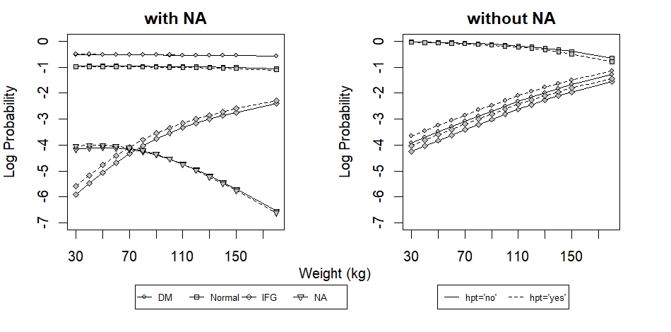
Figure 1: Log-scale Categorical Probability against Weight Based on Models with or without NA Category for the Metabolic Syndrome Dataset

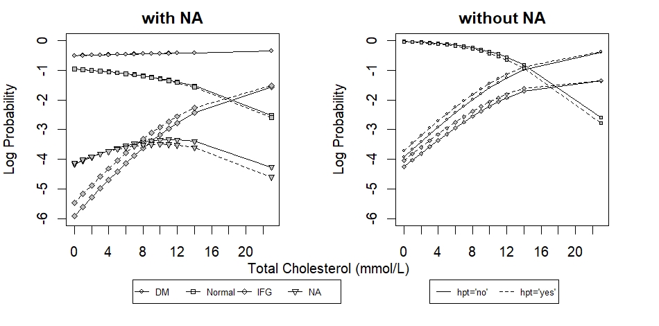
Figure 2: Log-scale Categorical Probability against Cholesterol Based on Models with or without NA Category for the Metabolic Syndrome Dataset

Figure 1 shows how $\log\hat{\pi}_{ij}$ changes against weight based on the fitted Model with or without the NA category. When weight increases, the probability of Normal or IFG category changes with a similarly pattern with or without NA. However, the patterns of DM category are quite different. If we remove the NA category, the conclusion would be that the risk of DM increases significantly along with weight; while with NA category included the risk of DM is fairly flat and seems not so relevant to weight. Similar story occurs for the risk of DM against cholesterol with or without NA (see Figure 2).

In other words, if we remove all observations with NA responses, we may conclude that both cholesterol and weight heavily affect the risk of DM; while with the complete data, the effects of cholesterol and weight are actually not that important. One possible explanation is that according to the Log Probability against weight with NA (see Figure 1, left panel), the chance of NA significantly decreases along with weight. In other words, the responses were not missing at random.

5.2 Trauma clinical trial with mixed-link models

In this section, we use a trauma clinical data discussed by Chuang-Stein and Agresti (1997) to show that the proposed mixed-link models (see Example 2.1) can be significantly better than the traditional logit models.

Chuang-Stein and Agresti (1997) studied a trauma clinical trial with $n=802$ of trauma patients with five ordered response categories, Death, Vegetative state, Major disability, Minor disability, and Good recovery, known as the Glasgow Outcome Scale (GOS) in the literature of critical care (Jennett and Bond, 1975). An extended dataset (Table V in Chuang-Stein and Agresti (1997)) consists of $802$ observations with two covariates, trauma severity ($x_{1}=0,1$) and dose level ($x_{2}=1,2,3,4$). In the literature, a main-effects cumulative logit model (2) with po was applied to this dataset (Chuang-Stein and Agresti, 1997), where the logit link was assumed for all categories.

In this study, we allow separate links for different categories and use a main-effects mixed-link model with po. For illustration purposes, we use logit, probit, loglog, and cloglog as our candidate set of link functions. The best model that we find for this dataset applies log-log, probit, log-log, and logit links to $j=1,2,3,4$, respectively. This multi-link model achieves BIC $198.43$, while the original logit model has a BIC value $252.74$.

To further show that the improvement is significant, we use five-fold cross-validations with cross-entropy loss (Hastie et al., 2009; Dousti Mousavi et al., 2023) and $200$ randomly generated partitions. As showed in Figure 3, our multi-link model is significantly better than the original logit model in terms of prediction accuracy.

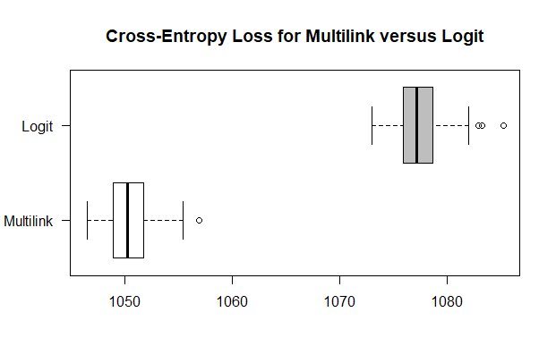
Figure 3: Boxplots of 5-Fold Cross-Validations with Cross-Entropy Loss and $200$ Random Partitions for Modeling Extended Trauma Data

5.3 Police data with po-npo mixture model

In this section, we use a police data discussed by Wang and Yang (2023) to show that the po-npo mixture model (see Example 2.3) can be significantly better than the traditional ppo models.

The police data (Wang and Yang, 2023) consists of summarized information of $n=12,483$ suspects’ Armed status (gun, other, or unarmed), Gender (0 or 1), Flee (0 or 1), Mental illness (0 or 1), as well as the responses of police with four categories, Tasered, Shot, Shot & Tasered, and Other, which do not have a natural ordering. According to Wang and Yang (2023), a continuation-ratio logit model (4) with npo and the working order $\{$Tasered, Shot, Other, Shot & Tasered$\}$ chosen by AIC is significantly better than the baseline-category models (1) or multiclass logistic model. The best model reported in Wang and Yang (2023) has the AIC value $192.01$.

To find the most appropriate po-npo mixture model, we run Algorithm 5 with iterations $t=1,\ldots,6$. The corresponding AIC values after the six iterations are $190.36,188.47,$ $187.96,187.04,185.04,186.07$, respectively. Since the $6$th iteration leads to an increased AIC value, then we report the fitted po-npo mixture model right after the $5$th iteration. The fitted parameters are listed in Table 2 with equal parameters per column in bold.

$j$	Intercept	Armed Status	Armed Status	Gender	Flee	Mental Illness
	$\hat{\beta}_{j1}$	$\hat{\beta}_{j2}$ (Other)	$\hat{\beta}_{j3}$ (Unarmed)	$\hat{\beta}_{j4}$	$\hat{\beta}_{j5}$	$\hat{\beta}_{j6}$
1	-5.987	-0.561	2.025	1.173	-10.958	1.328
2	6.655	-2.432	-1.089	-0.769	-1.552	-0.589
3	-1.784	-0.561	2.025	-0.769	-10.958	1.328

Table 2: Estimated Parameters for Police Data under Po-Npo Mixture Model

Compared with the AIC value $192.01$ of Wang and Yang (2023)’s npo model, the AIC value $185.04$ of the reported po-npo mixture model is significantly better according to Burnham and Anderson (2004).

5.4 House flies experiment with predictor selection

In this section, we use a house flies data discussed by Zocchi and Atkinson (1999) to show that the confidence intervals and hypothesis tests described in Section 3.4 can be used for predictor or variable selection.

Reported by Itepan (1995), the emergence of house flies data consists of summarized responses from $n=3,500$ pupae under a radiation experiment with the only covariate $x_{i}$, Dose of radiation. There are $J=3$ possible response categories, Unopened, Opened but died (before completing emergence), and Completed emergence, which have a nested or hierarchical structure.

Zocchi and Atkinson (1999) proposed a continuation-ratio logit model for the emergence of house flies data as follows (see also Bu et al. (2020)):

$$\log\left(\frac{\pi_{i1}}{\pi_{i2}+\pi_{i3}}\right)=\beta_{11}+\beta_{12}x_{i}+\beta_{13}x_{i}^{2},\>\>\>\log\left(\frac{\pi_{i2}}{\pi_{i3}}\right)=\beta_{21}+\beta_{22}x_{i}$$ (30)

where $x_{i}\in[80,200]$ is the radiation level in units Gy. By utilizing Algorithm 1, we obtain the fitted parameters $\hat{\boldsymbol{\beta}}=(\hat{\beta}_{11},\hat{\beta}_{12},\hat{\beta}_{13},\hat{\beta}_{21},\hat{\beta}_{22})^{T}=(-1.935,-0.02642,0.0003174,$ $-9.159,0.06386)^{T}$, which is consistent with the values reported in Zocchi and Atkinson (1999).

As described in Section 3.4, we further compute the Fisher information matrix ${\mathbf{F}}(\hat{\boldsymbol{\theta}})$, the confidence intervals of $\boldsymbol{\theta}$, and find that only the $95\%$ confidence interval $(-0.0541,$ $0.0013)$ for $\beta_{12}$ contains $0$, which implies a reduced continuation-ratio model as follows:

$$\log\left(\frac{\pi_{i1}}{\pi_{i2}+\pi_{i3}}\right)=\beta_{11}+\beta_{13}x_{i}^{2},\>\>\>\log\left(\frac{\pi_{i2}}{\pi_{i3}}\right)=\beta_{21}+\beta_{22}x_{i}$$ (31)

which is significantly better than Model (30). Actually, in terms of BIC values (see Section 3.5), Model (31)’s $108.17$ is also better than Model (30)’s $112.91$.

6 Conclusion

The proposed multinomial link model is much more flexible than existing multinomial models. It allows separate link functions for different categories (see Example 2.1) and more flexible model structures (see Example 2.3) than ppo models. More importantly, by arranging the response categories into two or more groups and finding working orders for each group, the proposed model can incorporate the observations with missing categorical responses into data analysis, which is often not missed at random. As shown in Section 5.1, the proposed two-group model can not only predict the probability or risk of a regular category, but also check if the NA category is due to randomness. In the example of metabolic syndrome data, it clearly shows that the chance of NA category decreases as weight increases, which is not at random.

The algorithms for finding the MLE and the formulae on computing the gradient and information matrix are developed for the unified form of (9) or (10), and are therefore applicable for all multinomial link models, including the mixed link models (Example 2.1), two-group models (Example 2.2), po-npo mixture models (Example 2.3), and others.

The proposed algorithms, especially Algorithms 1 and 3, solve the infeasibility issue of cumulative link models in existing statistics software. We also provide easy-to-use conditions (18) for general multinomial link models, which covers the classical cumulative link models as special cases.

SUPPLEMENTARY MATERIAL

S.1 More on mixed-link models:

Technical details that make mixed-link models a special class of multinomial link models;

S.2 More on two-group models:

Technical details that make two-group models a special class of multinomial link models;

S.3 More on Fisher information matrix:

Technical details on deriving Fisher information matrix;

S.4 Summary of notations for multinomial link models:

Summary of notations for specifying a multinomial link model;

S.5 Proofs:

Proofs for lemmas and theorems.

Ackowledgement The authors gratefully acknowledge the support from the U.S. NSF grant DMS-1924859.

Multinomial Link Models

Tianmeng Wang¹, Liping Tong², and Jie Yang¹

¹University of Illinois at Chicago and ²Advocate Aurora Health

Supplementary Materials

S.1 More on mixed-link models: Technical details that make mixed-link models a special class of multinomial link models;
S.2 More on two-group models: Technical details that make two-group models a special class of multinomial link models;
S.3 More on Fisher information matrix: Technical details on deriving Fisher information matrix;
S.4 Summary of notations for multinomial link models: Summary of notations for specifying a multinomial link model;
S.5 Proofs: Proofs for lemmas and theorems.

S.1 More on mixed-link models

The mixed-link models (12)+(13) introduced in Example 2.1 include four classes of models, baseline-category mixed-link models, cumulative mixed-link models, adjacent-categories mixed-link models, and continuation-ratio mixed-link models.

In this section, we show the technical details that make the mixed-link models (12)+(13) a special class of the multinomial link models (9) or (10).

By letting the model matrix ${\mathbf{X}}_{i}$ in (9) or (10) take the following specific form

$${\mathbf{X}}_{i}=\begin{pmatrix}{\mathbf{h}}_{1}^{T}({\mathbf{x}}_{i})&&&{\mathbf{h}}_{c}^{T}({\mathbf{x}}_{i})\\ &\ddots&&\vdots\\ &&{\mathbf{h}}_{J-1}^{T}({\mathbf{x}}_{i})&{\mathbf{h}}_{c}^{T}({\mathbf{x}}_{i})\end{pmatrix}\>\in\mathbb{R}^{(J-1)\times p}$$ (S.1)

with the regression parameter vector $\boldsymbol{\theta}=(\boldsymbol{\beta}_{1}^{T},\cdots,\boldsymbol{\beta}_{J-1}^{T},\boldsymbol{\zeta}^{T})^{T}$ consists of $p=p_{1}+\cdots+p_{J-1}+p_{c}$ unknown parameters in total, model (9) with ppo can be written as

$$g_{j}\left(\frac{{\mathbf{L}}^{T}_{j}\boldsymbol{\pi}_{i}}{{\mathbf{R}}^{T}_{j}\boldsymbol{\pi}_{i}+\pi_{iJ}b_{j}}\right)=\eta_{ij}={\mathbf{h}}_{j}^{T}({\mathbf{x}}_{i})\boldsymbol{\beta}_{j}+{\mathbf{h}}_{c}^{T}({\mathbf{x}}_{i})\boldsymbol{\zeta},\quad j=1,\ldots,J-1$$ (S.2)

In the rest of this section, we specify the $(J-1)\times(J-1)$ matrices ${\mathbf{L}}$, ${\mathbf{R}}$ and the vector ${\mathbf{b}}$ in model (9) (or equivalently the vectors ${\mathbf{L}}_{j}$, ${\mathbf{R}}_{j}$, and the numbers $b_{j}$ in model (10)) for each of the four classes of mixed-link models.

For facilitate the readers (see Step $3^{\circ}$ of Algorithm 4), we also provide the explicit formulae for ${\mathbf{D}}_{i}^{-1}$ and ${\mathbf{D}}_{i}^{-1}{\mathbf{b}}$, which are critical for computing the Fisher information matrix and the fitted categorical probabilities, where ${\mathbf{D}}_{i}={\rm diag}(\boldsymbol{\rho}_{i}^{-1}){\mathbf{L}}-{\mathbf{R}}$.

S.1.1 Baseline-category mixed-link models

In this case, ${\mathbf{L}}={\mathbf{R}}=I_{J-1}$, the identity matrix of order $J-1$, and ${\mathbf{b}}={\mathbf{1}}_{J-1}$, the vector of all ones with length $J-1$. A special case is $g_{1}=\cdots=g_{J-1}=g$. Then

$${\mathbf{D}}_{i}^{-1} = {\rm diag}\left(\boldsymbol{\rho}_{i}/(1-\boldsymbol{\rho}_{i})\right)={\rm diag}\left\{\frac{\rho_{i1}}{1-\rho_{i1}},\ldots,\frac{\rho_{i,J-1}}{1-\rho_{i,J-1}}\right\}$$

$${\mathbf{D}}_{i}^{-1}{\mathbf{b}} = \boldsymbol{\rho}_{i}/(1-\boldsymbol{\rho}_{i})=\left(\frac{\rho_{i1}}{1-\rho_{i1}},\ldots,\frac{\rho_{i,J-1}}{1-\rho_{i,J-1}}\right)^{T}$$

A special case is when $J=2$, $\boldsymbol{\rho}_{i}=\boldsymbol{\pi}_{i}=\pi_{i1}\in\mathbb{R}$.

S.1.2 Cumulative mixed-link models

In this case,

$${\mathbf{L}}=\left[\begin{array}[]{cccc}1&&&\\ 1&1&&\\ \vdots&\vdots&\ddots&\\ 1&1&\cdots&1\end{array}\right]\quad\in\mathbb{R}^{(J-1)\times(J-1)}$$

${\mathbf{R}}={\mathbf{1}}_{J-1}{\mathbf{1}}_{J-1}^{T}$, ${\mathbf{b}}={\mathbf{1}}_{J-1}$. A special case is $g_{1}=g_{2}=\cdots=g_{J-1}=g$. Then

$${\mathbf{D}}_{i}^{-1}=\left[\begin{array}[]{cccccc}\rho_{i1}&0&0&\cdots&0&\frac{\rho_{i,J-1}\rho_{i1}}{1-\rho_{i,J-1}}\\ -\rho_{i1}&\rho_{i2}&0&\cdots&0&\frac{\rho_{i,J-1}(\rho_{i2}-\rho_{i1})}{1-\rho_{i,J-1}}\\ 0&-\rho_{i2}&\rho_{i3}&\cdots&0&\frac{\rho_{i,J-1}(\rho_{i3}-\rho_{i2})}{1-\rho_{i,J-1}}\\ \vdots&\vdots&\vdots&\ddots&\vdots&\vdots\\ 0&0&0&\cdots&\rho_{i,J-2}&\frac{\rho_{i,J-1}(\rho_{i,J-2}-\rho_{i,J-3})}{1-\rho_{i,J-1}}\\ 0&0&0&\cdots&-\rho_{i,J-2}&\frac{\rho_{i,J-1}(1-\rho_{i,J-2})}{1-\rho_{i,J-1}}\end{array}\right]\quad\in\mathbb{R}^{(J-1)\times(J-1)}$$

exists, ${\mathbf{D}}_{i}^{-1}{\mathbf{b}}=(1-\rho_{i,J-1})^{-1}(\rho_{i1},\rho_{i2}-\rho_{i1},\ldots,$ $\rho_{i,J-2}-\rho_{i,J-3},$ $\rho_{i,J-1}-\rho_{i,J-2})^{T}$, and ${\mathbf{1}}_{J-1}^{T}{\mathbf{D}}_{i}^{-1}{\mathbf{b}}=\rho_{i,J-1}/(1-\rho_{i,J-1})$.

One special case is when $J=2$, $\boldsymbol{\rho}_{i}=\boldsymbol{\pi}_{i}=\pi_{i1}\in\mathbb{R}$.

Another special case is when $J=3$,

$${\mathbf{D}}_{i}^{-1}=\left[\begin{array}[]{cc}\rho_{i1}&\frac{\rho_{i2}\rho_{i1}}{1-\rho_{i2}}\\ -\rho_{i1}&\frac{\rho_{i2}(1-\rho_{i1})}{1-\rho_{i2}}\end{array}\right]\quad\in\mathbb{R}^{2\times 2}$$

exists, ${\mathbf{D}}_{i}^{-1}{\mathbf{b}}=(1-\rho_{i2})^{-1}(\rho_{i1},\rho_{i2}-\rho_{i1})^{T}$.

S.1.3 Adjacent-categories mixed-link models

In this case, ${\mathbf{L}}=I_{J-1}$,

$${\mathbf{R}}=\left[\begin{array}[]{ccccc}1&1&&&\\ &1&1&&\\ &&1&\ddots&\\ &&&\ddots&1\\ &&&&1\end{array}\right]\in\mathbb{R}^{(J-1)\times(J-1)},\quad{\mathbf{b}}=\left[\begin{array}[]{c}0\\ 0\\ \vdots\\ 0\\ 1\end{array}\right]\in\mathbb{R}^{J-1}$$

A special case is $g_{1}=\cdots=g_{J-1}=g$. Then ${\mathbf{D}}_{i}^{-1}=(a_{st})_{s,t=1,\ldots,J-1}$ exists with

$$a_{st}=\left\{\begin{array}[]{cl}\prod_{l=s}^{t}\frac{\rho_{il}}{1-\rho_{il}}&\mbox{ if }s\leq t\\ 0&\mbox{ if }s>t\end{array}\right.$$

All elements of

$${\mathbf{D}}_{i}^{-1}{\mathbf{b}}=\left(\prod_{l=1}^{J-1}\frac{\rho_{il}}{1-\rho_{il}},\ \prod_{l=2}^{J-1}\frac{\rho_{il}}{1-\rho_{il}},\ \ldots,\ \prod_{l=J-1}^{J-1}\frac{\rho_{il}}{1-\rho_{il}}\right)^{T}\in\mathbb{R}^{J-1}$$

are positive.

One special case is when $J=2$, ${\mathbf{L}}={\mathbf{R}}={\mathbf{b}}=1$ and then $\boldsymbol{\rho}_{i}=\boldsymbol{\pi}_{i}=\pi_{i1}\in\mathbb{R}$.

Remark S.1.1.

For adjacent-categories logit models, the vglm function in the R package VGAM calculates $\log\left(\frac{\pi_{i,j+1}}{\pi_{ij}}\right)$ instead of $\log\left(\frac{\pi_{ij}}{\pi_{i,j+1}}\right)$. This will lead to $\boldsymbol{\theta}$ discussed in our paper is different from $\boldsymbol{\theta}^{vglm}$ calculated from vglm function, but $\boldsymbol{\hat{\pi}}_{i}$ and log-likelihood will be the same for both $\boldsymbol{\theta}$ and $\boldsymbol{\theta}^{vglm}$.

S.1.4 Continuation-ratio mixed-link models

In this case, ${\mathbf{L}}=I_{J-1}$,

$${\mathbf{R}}=\left[\begin{array}[]{cccc}1&1&\cdots&1\\ &1&\cdots&1\\ &&\ddots&\vdots\\ &&&1\end{array}\right]\in\mathbb{R}^{(J-1)\times(J-1)}$$

${\mathbf{b}}={\mathbf{1}}_{J-1}$. A special case is $g_{1}=\cdots=g_{J-1}=g$. Then ${\mathbf{D}}_{i}^{-1}=(a_{st})_{s,t=1,\ldots,J-1}$ exists with

$$a_{st}=\left\{\begin{array}[]{cl}\rho_{is}\rho_{it}\prod_{l=s}^{t}(1-\rho_{il})^{-1}&\mbox{ if }s<t\\ \rho_{is}(1-\rho_{is})^{-1}&\mbox{ if }s=t\\ 0&\mbox{ if }s>t\end{array}\right.$$

All elements of

$${\mathbf{D}}_{i}^{-1}{\mathbf{b}}=\left(\frac{\rho_{i1}}{\prod_{l=1}^{J-1}(1-\rho_{il})},\ \frac{\rho_{i2}}{\prod_{l=2}^{J-1}(1-\rho_{il})},\ \ldots,\ \frac{\rho_{i,J-1}}{\prod_{l=J-1}^{J-1}(1-\rho_{il})}\right)^{T}\in\mathbb{R}^{J-1}$$

are positive. It can be verified that ${\mathbf{1}}_{J-1}^{T}{\mathbf{D}}_{i}^{-1}{\mathbf{b}}=\prod_{l=1}^{J-1}(1-\rho_{il})^{-1}-1$.

One special case is when $J=2$, $\boldsymbol{\rho}_{i}=\boldsymbol{\pi}_{i}=\pi_{i1}\in\mathbb{R}$.

S.2 More on two-group models

In this section, we show the technical details that make the two-group models (12)+(14) introduced in Example 2.2 a special class of the multinomial link models (9) or (10).

Similar as in Section S.1 for Example 2.1, the model matrix ${\mathbf{X}}_{i}$ in (9) or (10) take the form of (S.1); and the regression parameter vector $\boldsymbol{\theta}=(\boldsymbol{\beta}_{1}^{T},\cdots,\boldsymbol{\beta}_{J-1}^{T},\boldsymbol{\zeta}^{T})^{T}$ consists of $p=p_{1}+\cdots+p_{J-1}+p_{c}$ unknown parameters in total. Then model (9) can be written as (S.2).

In the rest of this section, we specify the $(J-1)\times(J-1)$ matrices ${\mathbf{L}}$, ${\mathbf{R}}$ and the vector ${\mathbf{b}}$ in model (9) (or equivalently the vectors ${\mathbf{L}}_{j}$, ${\mathbf{R}}_{j}$, and the numbers $b_{j}$ in model (10)) for each of the three classes of two-group models. Similarly as in Section S.1 for Example 2.1, we also provide the explicit formulae for ${\mathbf{D}}_{i}^{-1}$ and ${\mathbf{D}}_{i}^{-1}{\mathbf{b}}$.

First, we focus on a special class of two-group models whose two groups share the same baseline category $J$. That is, $s=J$ in this case, which leads to simplified notations.

Example S.2.1.

Two-group models with shared baseline category Under (12), the same form as in the mixed-link models (Example 2.1), we further assume that there exists an integer $k$, such that, $1\leq k\leq J-3$ and

$$\rho_{ij}=\left\{\begin{array}[]{cl}\frac{\pi_{ij}}{\pi_{ij}+\pi_{iJ}}&\mbox{ for }j=1,\ldots,k\\ \frac{\pi_{i,k+1}+\cdots+\pi_{ij}}{\pi_{i,k+1}+\cdots+\pi_{iJ}}&\mbox{ for baseline-cumulative and }j=k+1,\ldots,J-1\\ \frac{\pi_{ij}}{\pi_{ij}+\pi_{i,j+1}}&\mbox{ for baseline-adjacent and }j=k+1,\ldots,J-1\\ \frac{\pi_{ij}}{\pi_{ij}+\cdots+\pi_{iJ}}&\mbox{ for baseline-continuation and }j=k+1,\ldots,J-1\end{array}\right.$$ (S.3)

It indicates that the response categories form two groups, $\{1,\ldots,k,J\}$ and $\{k+1,\ldots,J-1,J\}$, which share the same baseline category $J$.

The two-group models (12)+(S.3) also consist of three classes, baseline-cumulative, baseline-adjacent, and baseline-continuation mixed-link models with shared baseline category, which are all special cases of the multinomial link models (9) or (10) (see Sections S.2.1, S.2.2, and S.2.3). $\Box$

S.2.1 Baseline-cumulative mixed-link models with shared baseline category

There are two groups of response categories in this model. One group of $k+1\geq 2$ categories are controlled by a baseline-category mixed-link model and the other group of $J-k\geq 3$ categories are controlled by a cumulative mixed-link model. The two groups share the same baseline category $J$. More specifically, let $1\leq k\leq J-3$ and

$$\rho_{ij}=\left\{\begin{array}[]{cl}\frac{\pi_{ij}}{\pi_{ij}+\pi_{iJ}}&\mbox{ for }j=1,\ldots,k\\ \frac{\pi_{i,k+1}+\cdots+\pi_{ij}}{\pi_{i,k+1}+\cdots+\pi_{iJ}}&\mbox{ for }j=k+1,\ldots,J-1\end{array}\right.$$

As for link functions, a special case is $g_{1}=\cdots=g_{k}=g_{a}$ and $g_{k+1}=\cdots=g_{J-1}=g_{b}$ . Then

$${\mathbf{L}}=\left[\begin{array}[]{ccccc}I_{k}&&&&\\ &1&&&\\ &1&1&&\\ &\vdots&\vdots&\ddots&\\ &1&1&\cdots&1\end{array}\right],\>\>\>{\mathbf{R}}=\left[\begin{array}[]{ccccc}I_{k}&&&&\\ &1&1&\cdots&1\\ &1&1&\cdots&1\\ &\vdots&\vdots&\ddots&\vdots\\ &1&1&\cdots&1\end{array}\right]$$

${\mathbf{b}}={\mathbf{1}}_{J-1}$. Then

$${\mathbf{D}}_{i}^{-1}=\left[\begin{array}[]{ccccccccc}\frac{\rho_{i1}}{1-\rho_{i1}}&&&&&&&&\\ &\ddots&&&&&&&\\ &&\frac{\rho_{ik}}{1-\rho_{ik}}&&&&&&\\ &&&\rho_{i,k+1}&0&0&\cdots&0&\frac{\rho_{i,J-1}\rho_{i,k+1}}{1-\rho_{i,J-1}}\\ &&&-\rho_{i,k+1}&\rho_{i,k+2}&0&\cdots&0&\frac{\rho_{i,J-1}(\rho_{i,k+2}-\rho_{i,k+1})}{1-\rho_{i,J-1}}\\ &&&0&-\rho_{i,k+2}&\rho_{i,k+3}&\cdots&0&\frac{\rho_{i,J-1}(\rho_{i,k+3}-\rho_{i,k+2})}{1-\rho_{i,J-1}}\\ &&&\vdots&\vdots&\vdots&\ddots&\vdots&\vdots\\ &&&0&0&0&\cdots&\rho_{i,J-2}&\frac{\rho_{i,J-1}(\rho_{i,J-2}-\rho_{i,J-3})}{1-\rho_{i,J-1}}\\ &&&0&0&0&\cdots&-\rho_{i,J-2}&\frac{\rho_{i,J-1}(1-\rho_{i,J-2})}{1-\rho_{i,J-1}}\end{array}\right]$$

$${\mathbf{D}}_{i}^{-1}{\mathbf{b}} = \left(\frac{\rho_{i1}}{1-\rho_{i1}},\ldots,\frac{\rho_{ik}}{1-\rho_{ik}},\frac{\rho_{i,k+1}}{1-\rho_{i,J-1}},\frac{\rho_{i,k+2}-\rho_{i,k+1}}{1-\rho_{i,J-1}},\ldots,\frac{\rho_{i,J-1}-\rho_{i,J-2}}{1-\rho_{i,J-1}}\right)^{T}$$

$${\mathbf{1}}_{J-1}^{T}{\mathbf{D}}_{i}^{-1}{\mathbf{b}} = \sum_{l=1}^{k}\frac{\rho_{il}}{1-\rho_{il}}+\frac{\rho_{i,J-1}}{1-\rho_{i,J-1}}$$

One special case is when $J=4$ and $k=1$,

$${\mathbf{D}}_{i}^{-1}=\left[\begin{array}[]{ccc}\frac{\rho_{i1}}{1-\rho_{i1}}&&\\ &\rho_{i2}&\frac{\rho_{i3}\rho_{i2}}{1-\rho_{i3}}\\ &-\rho_{i2}&\frac{\rho_{i3}(1-\rho_{i2})}{1-\rho_{i3}}\end{array}\right]$$

S.2.2 Baseline-adjacent mixed-link models with shared baseline category

There are two groups of response categories in this model. One group of $k+1\geq 2$ categories are controlled by a baseline-category mixed-link model and the other group of $J-k\geq 3$ categories are controlled by an adjacent-categories mixed-link model. The two groups share the same baseline category $J$. More specifically, let $1\leq k\leq J-3$ and

$$\rho_{ij}=\left\{\begin{array}[]{cl}\frac{\pi_{ij}}{\pi_{ij}+\pi_{iJ}}&\mbox{ for }j=1,\ldots,k\\ \frac{\pi_{ij}}{\pi_{ij}+\pi_{i,j+1}}&\mbox{ for }j=k+1,\ldots,J-1\end{array}\right.$$

As for link functions, a special case is $g_{1}=\cdots=g_{k}=g_{a}$ and $g_{k+1}=\cdots=g_{J-1}=g_{b}$ . Then ${\mathbf{L}}=I_{J-1}$,

$${\mathbf{R}}=\left[\begin{array}[]{cccccc}I_{k}&&&&&\\ &1&1&&&\\ &&1&1&&\\ &&&1&\ddots&\\ &&&&\ddots&1\\ &&&&&1\end{array}\right]\in\mathbb{R}^{(J-1)\times(J-1)},\quad{\mathbf{b}}=\left[\begin{array}[]{c}{\mathbf{1}}_{k}\\ 0\\ \vdots\\ 0\\ 1\end{array}\right]\in\mathbb{R}^{J-1}$$

Then

$${\mathbf{D}}_{i}^{-1}=\left[\begin{array}[]{cccccccc}\frac{\rho_{i1}}{1-\rho_{i1}}&&&&&&&\\ &\ddots&&&&&&\\ &&\frac{\rho_{ik}}{1-\rho_{ik}}&&&&&\\ &&&\prod_{l=k+1}^{k+1}\frac{\rho_{il}}{1-\rho_{il}}&\prod_{l=k+1}^{k+2}\frac{\rho_{il}}{1-\rho_{il}}&\cdots&\prod_{l=k+1}^{J-2}\frac{\rho_{il}}{1-\rho_{il}}&\prod_{l=k+1}^{J-1}\frac{\rho_{il}}{1-\rho_{il}}\\ &&&&\prod_{l=k+2}^{k+2}\frac{\rho_{il}}{1-\rho_{il}}&\cdots&\prod_{l=k+2}^{J-2}\frac{\rho_{il}}{1-\rho_{il}}&\prod_{l=k+2}^{J-1}\frac{\rho_{il}}{1-\rho_{il}}\\ &&&&&\ddots&\vdots&\vdots\\ &&&&&&\prod_{l=J-2}^{J-2}\frac{\rho_{il}}{1-\rho_{il}}&\prod_{l=J-2}^{J-1}\frac{\rho_{il}}{1-\rho_{il}}\\ &&&&&&&\prod_{l=J-1}^{J-1}\frac{\rho_{il}}{1-\rho_{il}}\end{array}\right]$$

All elements of

$${\mathbf{D}}_{i}^{-1}{\mathbf{b}}=\left(\frac{\rho_{i1}}{1-\rho_{i1}},\ \cdots,\ \frac{\rho_{ik}}{1-\rho_{ik}},\ \prod_{l=k+1}^{J-1}\frac{\rho_{il}}{1-\rho_{il}},\ \ldots,\ \prod_{l=J-1}^{J-1}\frac{\rho_{il}}{1-\rho_{il}}\right)^{T}\in\mathbb{R}^{J-1}$$

are positive.

S.2.3 Baseline-continuation mixed-link models with shared baseline category

There are two groups of response categories in this model. One group of $k+1\geq 2$ categories are controlled by a baseline-category mixed-link model and the other group of $J-k\geq 3$ categories are controlled by a continuation-ratio mixed-link model. The two groups share the same baseline category $J$. More specifically, let $1\leq k\leq J-3$ and

$$\rho_{ij}=\left\{\begin{array}[]{cl}\frac{\pi_{ij}}{\pi_{ij}+\pi_{iJ}}&\mbox{ for }j=1,\ldots,k\\ \frac{\pi_{ij}}{\pi_{ij}+\cdots+\pi_{iJ}}&\mbox{ for }j=k+1,\ldots,J-1\end{array}\right.$$

As for link functions, a special case is $g_{1}=\cdots=g_{k}=g_{a}$ and $g_{k+1}=\cdots=g_{J-1}=g_{b}$ . Then ${\mathbf{L}}=I_{J-1}$,

$${\mathbf{R}}=\left[\begin{array}[]{ccccc}I_{k}&&&&\\ &1&1&\cdots&1\\ &&1&\cdots&1\\ &&&\ddots&\vdots\\ &&&&1\end{array}\right]\in\mathbb{R}^{(J-1)\times(J-1)}$$

${\mathbf{b}}={\mathbf{1}}_{J-1}$. Then

$${\mathbf{D}}_{i}^{-1}=\left[\begin{array}[]{cccccccc}\frac{\rho_{i1}}{1-\rho_{i1}}&&&&&&&\\ &\ddots&&&&&&\\ &&\frac{\rho_{ik}}{1-\rho_{ik}}&&&&&\\ &&&\frac{\rho_{i,k+1}}{\prod_{l=k+1}^{k+1}(1-\rho_{il})}&\frac{\rho_{i,k+1}\rho_{i,k+2}}{\prod_{l=k+1}^{k+2}(1-\rho_{il})}&\cdots&\frac{\rho_{i,k+1}\rho_{i,J-2}}{\prod_{l=k+1}^{J-2}(1-\rho_{il})}&\frac{\rho_{i,k+1}\rho_{i,J-1}}{\prod_{l=k+1}^{J-1}(1-\rho_{il})}\\ &&&&\frac{\rho_{i,k+2}}{\prod_{l=k+2}^{k+2}(1-\rho_{il})}&\cdots&\frac{\rho_{i,k+2}\rho_{i,J-2}}{\prod_{l=k+2}^{J-2}(1-\rho_{il})}&\frac{\rho_{i,k+2}\rho_{i,J-1}}{\prod_{l=k+2}^{J-1}(1-\rho_{il})}\\ &&&&&\ddots&\vdots&\vdots\\ &&&&&&\frac{\rho_{i,J-2}}{\prod_{l=J-2}^{J-2}(1-\rho_{il})}&\frac{\rho_{i,J-2}\rho_{i,J-1}}{\prod_{l=J-2}^{J-1}(1-\rho_{il})}\\ &&&&&&&\frac{\rho_{i,J-1}}{\prod_{l=J-1}^{J-1}(1-\rho_{il})}\end{array}\right]$$

All elements of

$${\mathbf{D}}_{i}^{-1}{\mathbf{b}}=\left(\frac{\rho_{i1}}{1-\rho_{i1}},\ \ldots,\ \frac{\rho_{ik}}{1-\rho_{ik}},\ \frac{\rho_{i,k+1}}{\prod_{l=k+1}^{J-1}(1-\rho_{il})},\ \ldots,\ \frac{\rho_{i,J-1}}{\prod_{l=J-1}^{J-1}(1-\rho_{il})}\right)^{T}\in\mathbb{R}^{J-1}$$

are positive. It can be verified that

$${\mathbf{1}}_{J-1}^{T}{\mathbf{D}}_{i}^{-1}{\mathbf{b}}=\sum_{l=1}^{k}\frac{\rho_{il}}{1-\rho_{il}}+\prod_{l=k+1}^{J-1}(1-\rho_{il})^{-1}-1$$

S.2.4 More on two-group models in Example 2.2

For the two-group model introduced in Example 2.2, the ${\mathbf{L}}$ matrix is exactly the same as in Section S.2.1, S.2.2 and S.2.3 for the corresponding link models. The ${\mathbf{R}}$ matrix can be obtained by adding more $1$’s to the corresponding ${\mathbf{R}}$ matrix in Section S.2.1, S.2.2 or S.2.3. More specifically, we only need to change the $0$’s at the $(1,s),(2,s),\ldots,(k,s)$th entries of ${\mathbf{R}}$ to $1$’s.

The vector ${\mathbf{b}}=(b_{1},\ldots,b_{J-1})^{T}$ is quite different though. Actually,

$${\mathbf{b}}=\left\{\begin{array}[]{cl}({\mathbf{0}}_{k}^{T},{\mathbf{1}}_{J-k-1}^{T})^{T}&\mbox{ for baseline-cumulative}\\ ({\mathbf{0}}_{J-2}^{T},1)^{T}&\mbox{ for baseline-adjacent}\\ ({\mathbf{0}}_{k}^{T},{\mathbf{1}}_{J-k-1}^{T})^{T}&\mbox{ for baseline-continuation}\end{array}\right.$$

where ${\mathbf{0}}_{k}=(0,\ldots,0)^{T}\in\mathbb{R}^{k}$ and ${\mathbf{1}}_{k}=(1,\ldots,1)^{T}\in\mathbb{R}^{k}$.

As an illustrative example, a baseline-cumulative mixed-link model with $J=5$, $k=1$, and $s=3$ has two groups of categories $\{1,3\}$ (with baseline $3$) and $\{2,3,4,5\}$ (with baseline $5$), as well as

$${\mathbf{L}}=\left[\begin{array}[]{cccc}1&&&\\ &1&&\\ &1&1&\\ &1&1&1\end{array}\right],\>\>\>{\mathbf{R}}=\left[\begin{array}[]{cccc}1&&1&\\ &1&1&1\\ &1&1&1\\ &1&1&1\end{array}\right],\>\>\>{\mathbf{b}}=\left(\begin{array}[]{c}0\\ 1\\ 1\\ 1\end{array}\right)$$

S.3 More on Fisher information matrix

In this section, we provide more technical details about Section 3.2.

Recall that given distinct ${\mathbf{x}}_{i},i=1,\cdots,m$, we have independent multinomial responses

$${\mathbf{Y}}_{i}=(Y_{i1},\cdots,Y_{iJ})^{T}\sim{\rm Multinomial}(n_{i};\pi_{i1},\cdots,\pi_{iJ})$$

where $n_{i}=\sum_{j=1}^{J}Y_{ij}$. The log-likelihood for the multinomial model is

$$l(\boldsymbol{\theta})=\log\prod_{i=1}^{m}\frac{{n_{i}}!}{{Y_{i1}}!\cdots{Y_{iJ}}!}\pi_{i1}^{Y_{i1}}\cdots\pi_{iJ}^{Y_{iJ}}=\sum_{i=1}^{m}{\mathbf{Y}}_{i}^{T}\log\bar{\boldsymbol{\pi}}_{i}+\sum_{i=1}^{m}\log(n_{i}!)-\sum_{i=1}^{m}\sum_{j=1}^{J}\log(Y_{ij}!)$$

where $\bar{\boldsymbol{\pi}}_{i}=(\pi_{i1},\ldots,\pi_{iJ})^{T}=(\boldsymbol{\pi}_{i}^{T},\pi_{iJ})^{T}$, $\log\bar{\boldsymbol{\pi}}_{i}=(\log\pi_{i1},\cdots,\log\pi_{iJ})^{T}$.

Recall that $g_{1}^{-1},\ldots,g_{J-1}^{-1}$ are all differentiable. Then the score vector

$$\frac{\partial l}{\partial\boldsymbol{\theta}^{T}}=\sum_{i=1}^{m}{\mathbf{Y}}_{i}^{T}{\rm diag}(\bar{\boldsymbol{\pi}}_{i})^{-1}\frac{\partial\bar{\boldsymbol{\pi}}_{i}}{\partial\boldsymbol{\theta}^{T}}$$

with

$$\frac{\partial\bar{\boldsymbol{\pi}}_{i}}{\partial\boldsymbol{\theta}^{T}}=\frac{\partial\bar{\boldsymbol{\pi}}_{i}}{\partial\boldsymbol{\rho}_{i}^{T}}\cdot\frac{\partial\boldsymbol{\rho}_{i}}{\partial\boldsymbol{\eta}_{i}^{T}}\cdot\frac{\partial\boldsymbol{\eta}_{i}}{\partial\boldsymbol{\theta}^{T}}\\ =\frac{\partial\bar{\boldsymbol{\pi}}_{i}}{\partial\boldsymbol{\rho}_{i}^{T}}\cdot{\rm diag}\left(\left({\mathbf{g}}^{-1}\right)^{\prime}\left(\boldsymbol{\eta}_{i}\right)\right)\cdot{\mathbf{X}}_{i}$$

where $\boldsymbol{\rho}_{i}=(\rho_{i1},\ldots,\rho_{i,J-1})^{T}\in\mathbb{R}^{J-1}$, $\boldsymbol{\eta}_{i}=(\eta_{i1},$ $\ldots,$ $\eta_{i,J-1})^{T}$ $\in$ $\mathbb{R}^{J-1}$, ${\rm diag}\left(\left({\mathbf{g}}^{-1}\right)^{\prime}\left(\boldsymbol{\eta}_{i}\right)\right)={\rm diag}\left\{\left(g_{1}^{-1}\right)^{\prime}\left(\eta_{i1}\right),\ldots,\left(g_{J-1}^{-1}\right)^{\prime}\left(\eta_{i,J-1}\right)\right\}\in\mathbb{R}^{(J-1)\times(J-1)}$. As for $\partial\bar{\boldsymbol{\pi}}_{i}/\partial\boldsymbol{\rho}_{i}^{T}$, Lemma S.3.1 provides a formula for $\partial\boldsymbol{\pi}_{i}/\partial\boldsymbol{\rho}_{i}^{T}$.

Lemma S.3.1.

Suppose $\boldsymbol{\theta}\in\boldsymbol{\Theta}$. Then

$$\frac{\partial\boldsymbol{\pi}_{i}}{\partial\boldsymbol{\rho}_{i}^{T}}=\left(I_{J-1}-\boldsymbol{\pi}_{i}{\mathbf{1}}_{J-1}^{T}\right){\mathbf{D}}_{i}^{-1}\cdot{\rm diag}\left({\mathbf{L}}\boldsymbol{\pi}_{i}\right)\cdot{\rm diag}\left(\boldsymbol{\rho}_{i}^{-2}\right)$$

$\Box$

Proof of Lemma S.3.1: Applying the chain rule of vector differentiation and matrix differentials (see, for example, Chapter 17 in Seber (2008)) to (17), we obtain

$$\frac{\partial\boldsymbol{\pi}_{i}}{\partial\boldsymbol{\rho}_{i}^{T}} = \frac{\partial\boldsymbol{\pi}_{i}}{\partial({\mathbf{D}}_{i}^{-1}{\mathbf{b}})^{T}}\cdot\frac{\partial({\mathbf{D}}_{i}^{-1}{\mathbf{b}})}{\partial\boldsymbol{\rho}_{i}^{T}}$$

$$= \frac{1}{1+{\mathbf{1}}^{T}_{J-1}{\mathbf{D}}_{i}^{-1}{\mathbf{b}}}\left(I_{J-1}-\boldsymbol{\pi}_{i}{\mathbf{1}}_{J-1}^{T}\right)\cdot{\mathbf{D}}_{i}^{-1}{\rm diag}\left({\mathbf{L}}{\mathbf{D}}_{i}^{-1}{\mathbf{b}}\right){\rm diag}\left(\boldsymbol{\rho}_{i}^{-2}\right)$$

$$= \left(I_{J-1}-\boldsymbol{\pi}_{i}{\mathbf{1}}_{J-1}^{T}\right)\cdot{\mathbf{D}}_{i}^{-1}{\rm diag}\left({\mathbf{L}}\boldsymbol{\pi}_{i}\right){\rm diag}\left(\boldsymbol{\rho}_{i}^{-2}\right)$$

$\Box$

Since $\pi_{iJ}=1-{\mathbf{1}}_{J-1}^{T}\boldsymbol{\pi}_{i}$,

$$\frac{\partial\pi_{iJ}}{\partial\boldsymbol{\rho}_{i}^{T}}=-{\mathbf{1}}_{J-1}^{T}\frac{\partial\boldsymbol{\pi}_{i}}{\partial\boldsymbol{\rho}_{i}^{T}}=\left({\mathbf{0}}_{J-1}^{T}-\pi_{iJ}{\mathbf{1}}_{J-1}^{T}\right){\mathbf{D}}_{i}^{-1}\cdot{\rm diag}\left({\mathbf{L}}\boldsymbol{\pi}_{i}\right)\cdot{\rm diag}\left(\boldsymbol{\rho}_{i}^{-2}\right)$$

By combining $\partial\boldsymbol{\pi}_{i}/\partial\boldsymbol{\rho}_{i}^{T}$ and $\partial\pi_{iJ}/\partial\boldsymbol{\rho}_{i}^{T}$, we obtain

$$\frac{\partial\bar{\boldsymbol{\pi}}_{i}}{\partial\boldsymbol{\rho}_{i}^{T}}={\mathbf{E}}_{i}{\mathbf{D}}_{i}^{-1}\cdot{\rm diag}\left({\mathbf{L}}\boldsymbol{\pi}_{i}\right)\cdot{\rm diag}\left(\boldsymbol{\rho}_{i}^{-2}\right)$$ (S.4)

where ${\mathbf{E}}_{i}$ is defined in (25).

Lemma S.3.2.

$\bar{\boldsymbol{\pi}}_{i}^{T}{\rm diag}(\bar{\boldsymbol{\pi}}_{i})^{-1}{\mathbf{E}}_{i}={\mathbf{1}}_{J}^{T}{\mathbf{E}}_{i}={\mathbf{0}}$. $\Box$

Proof of Lemma S.3.2: Since $\pi_{i1}+\cdots+\pi_{iJ}=1$, then $\bar{\boldsymbol{\pi}}_{i}^{T}{\rm diag}(\bar{\boldsymbol{\pi}}_{i})^{-1}{\mathbf{E}}_{i}={\mathbf{1}}_{J}^{T}{\mathbf{E}}_{i}={\mathbf{1}}_{J-1}^{T}-{\mathbf{1}}_{J-1}^{T}={\mathbf{0}}_{J-1}^{T}$. $\Box$

Since the product of two diagonal matrices is exchangeable, then

$${\rm diag}\left({\mathbf{L}}\boldsymbol{\pi}_{i}\right)\cdot{\rm diag}\left(\boldsymbol{\rho}_{i}^{-2}\right)={\rm diag}\left((1-\boldsymbol{\rho}_{i})/\boldsymbol{\rho}_{i}\right)\cdot{\rm diag}\left({\mathbf{L}}\boldsymbol{\pi}_{i}\right)\cdot{\rm diag}\left(\boldsymbol{\rho}_{i}(1-\boldsymbol{\rho}_{i})\right)^{-1}$$

where ${\rm diag}\left((1-\boldsymbol{\rho}_{i})/\boldsymbol{\rho}_{i}\right)={\rm diag}\left\{(1-\rho_{i1})/\rho_{i1},\ldots,(1-\rho_{i,J-1})/\rho_{i,J-1}\right\}$ and
${\rm diag}\left(\boldsymbol{\rho}_{i}(1-\boldsymbol{\rho}_{i})\right)^{-1}={\rm diag}\left\{\rho_{i1}^{-1}(1-\rho_{i1})^{-1},\ldots,\rho_{i,J-1}^{-1}(1-\rho_{i,J-1})^{-1}\right\}$. Thus an equivalent formula of (S.4) is

$$\frac{\partial\bar{\boldsymbol{\pi}}_{i}}{\partial\boldsymbol{\rho}_{i}^{T}}={\mathbf{E}}_{i}{\mathbf{D}}_{i}^{-1}\cdot{\rm diag}\left(\frac{1-\boldsymbol{\rho}_{i}}{\boldsymbol{\rho}_{i}}\right)\cdot{\rm diag}\left({\mathbf{L}}\boldsymbol{\pi}_{i}\right)\cdot{\rm diag}\left(\boldsymbol{\rho}_{i}(1-\boldsymbol{\rho}_{i})\right)^{-1}$$

It can be verified that ${\mathbf{E}}_{i}{\mathbf{D}}_{i}^{-1}\cdot{\rm diag}\left((1-\boldsymbol{\rho}_{i})/\boldsymbol{\rho}_{i}\right)\cdot{\rm diag}\left({\mathbf{L}}\boldsymbol{\pi}_{i}\right)$ is consistent with the first $(J-1)$ columns of $\left({\mathbf{C}}^{T}{\mathbf{D}}_{i}^{-1}{\mathbf{L}}\right)^{-1}$ in Bu et al. (2020) for multinomial logitistic models, although their notations ${\mathbf{D}}_{i}$ and ${\mathbf{L}}$ are different from here. Therefore, Lemma S.5 in the Supplementary Materials of Bu et al. (2020) is a direct conclusion of Lemma S.3.2 here.

As another direct conclusion of Lemma S.3.2,

$$E\left(\frac{\partial l}{\partial\boldsymbol{\theta}^{T}}\right)=\sum_{i=1}^{m}n_{i}\bar{\boldsymbol{\pi}}_{i}^{T}{\rm diag}(\bar{\boldsymbol{\pi}}_{i})^{-1}\frac{\partial\bar{\boldsymbol{\pi}}_{i}}{\partial\boldsymbol{\theta}^{T}}={\mathbf{0}}$$

S.4 Summary of notations for multinomial link models

In this section, we summarize the notations for specifying a multinomial link model.

A general multinomial link model takes its matrix form as in (9) or its equation form as in (10). It consists of two components. The left hand side $g_{j}\left(\frac{{\mathbf{L}}^{T}_{j}\boldsymbol{\pi}_{i}}{{\mathbf{R}}^{T}_{j}\boldsymbol{\pi}_{i}+\pi_{iJ}b_{j}}\right)$ of (10) indicates the model is a baseline-category mixed-link model (see Section S.1.1), a cumulative mixed-link model (see Section S.1.2), an adjacent-categories mixed-link model (see Section S.1.3), a continuation-ratio mixed-link model (see Section S.1.4), a baseline-cumulative mixed-link model (see Section S.2.1), a baseline-adjacent mixed-link model (see Section S.2.2), a baseline-continuation mixed-link model (see Section S.2.3), or others. The right hand side ${\mathbf{f}}_{j}^{T}({\mathbf{x}}_{i})\boldsymbol{\theta}$ of (10) indicates that the model is with proportional odds (po, with $\beta_{j}+{\mathbf{h}}_{c}^{T}({\mathbf{x}}_{i})\boldsymbol{\zeta}$, $j=1,\ldots,J-1$), nonproportional odds (npo, with ${\mathbf{h}}_{j}^{T}({\mathbf{x}}_{i})\boldsymbol{\beta}_{j}$), partial proportional odds (ppo, with ${\mathbf{h}}_{j}^{T}({\mathbf{x}}_{i})\boldsymbol{\beta}_{j}+{\mathbf{h}}_{c}^{T}({\mathbf{x}}_{i})\boldsymbol{\zeta}$, see Example 3.1), po-npo mixture (with ${\mathbf{h}}_{j}^{T}({\mathbf{x}}_{i})\boldsymbol{\beta}_{j}+{\mathbf{h}}_{cj}^{T}({\mathbf{x}}_{i})\boldsymbol{\zeta}$, see Example 2.3), or other structures. Overall, the model is called, for example, a cumulative mixed-link model with proportional odds, a baseline-cumulative mixed-link model with po-npo mixture, etc. To specify such a model, we need to know

• Constant matrices ${\mathbf{L}},{\mathbf{R}}\in\mathbb{R}^{(J-1)\times(J-1)}$ and constant vector ${\mathbf{b}}\in\mathbb{R}^{J-1}$;

• Link functions $g_{1},\ldots,g_{J-1}$, as well as their inverses $g_{1}^{-1},\ldots,g_{J-1}^{-1}$ and the corresponding first-order derivatives $(g_{1}^{-1})^{\prime},\ldots,(g_{J-1}^{-1})^{\prime}$ (see Table 1 for relevant formulae);

• Predictor functions ${\mathbf{f}}_{j}({\mathbf{x}}_{i})=(f_{j1}({\mathbf{x}}_{i}),\ldots,f_{jp}({\mathbf{x}}_{i}))^{T}$ with $\boldsymbol{\theta}=(\theta_{1},\ldots,\theta_{p})^{T}$ in general; ${\mathbf{h}}_{j}({\mathbf{x}}_{i})=(h_{j1}({\mathbf{x}}_{i}),\ldots,h_{jp_{j}}({\mathbf{x}}_{i}))^{T}$, $j=1,\ldots,J-1$ and ${\mathbf{h}}_{c}({\mathbf{x}}_{i})=(h_{1}({\mathbf{x}}_{i}),\ldots,$ $h_{p_{c}}({\mathbf{x}}_{i}))^{T}$ or ${\mathbf{h}}_{cj}({\mathbf{x}}_{i})=(h_{cj1}({\mathbf{x}}_{i}),\ldots,h_{cjp_{c}}({\mathbf{x}}_{i}))^{T}$ with parameters $\boldsymbol{\theta}=(\boldsymbol{\beta}_{1}^{T},$ $\ldots,\boldsymbol{\beta}_{J-1}^{T},$ $\boldsymbol{\zeta}^{T})^{T}\in\mathbb{R}^{p_{1}+\cdots+p_{J-1}+p_{c}}$ for ppo model or po-npo mixture model; ${\mathbf{h}}_{j}({\mathbf{x}}_{i})\equiv 1$, $j=1,\ldots,J-1$, $p_{1}=\cdots=p_{J-1}=1$ with $\boldsymbol{\theta}=(\beta_{1},\ldots,\beta_{J-1},$ $\boldsymbol{\zeta}^{T})^{T}\in\mathbb{R}^{J-1+p_{c}}$ for po models; ${\mathbf{h}}_{c}({\mathbf{x}}_{i})\equiv 0$, $p_{c}=0$ and $\boldsymbol{\theta}=(\boldsymbol{\beta}_{1}^{T},\ldots,\boldsymbol{\beta}_{J-1}^{T})^{T}\in\mathbb{R}^{p_{1}+\cdots+p_{J-1}}$ for npo models.

Once (i), (ii) and (iii) are given, the model is specified. We can further calculate

• The model matrix ${\mathbf{X}}_{i}\in\mathbb{R}^{(J-1)\times p}$ according to (27) for general models. Special cases include (15) for po-npo mixture model (see Example 2.3), (S.1) for ppo model,

  $${\mathbf{X}}_{i}=\begin{pmatrix}1&&&{\mathbf{x}}_{i}^{T}\\ &\ddots&&\vdots\\ &&1&{\mathbf{x}}_{i}^{T}\end{pmatrix}\>\in\mathbb{R}^{(J-1)\times(d+J-1)}$$

  for main-effects po models (in this case, $p_{1}=\cdots=p_{J-1}=1$, $p_{c}=d$, $p=d+J-1$),

  $${\mathbf{X}}_{i}=\begin{pmatrix}1\ {\mathbf{x}}_{i}^{T}&&\\ &\ddots&\\ &&1\ {\mathbf{x}}_{i}^{T}\end{pmatrix}\>\in\mathbb{R}^{(J-1)\times(d+1)(J-1)}$$

  for main-effects npo models (in this case, $p_{1}=\cdots=p_{J-1}=d+1$, $p_{c}=0$, $p=(d+1)(J-1)$).

S.5 Proofs

Proof of Lemma 3.1

Since $\boldsymbol{\rho}_{i}=\left({\mathbf{L}}{\boldsymbol{\pi}}_{i}\right)/\left({\mathbf{R}}\boldsymbol{\pi}_{i}+\pi_{iJ}{\mathbf{b}}\right)$ and $\pi_{iJ}=1-\pi_{i1}-\cdots-\pi_{i,J-1}=1-{\mathbf{1}}_{J-1}^{T}\boldsymbol{\pi}_{i}$, we have

$${\mathbf{L}}{\boldsymbol{\pi}}_{i}={\rm diag}\left(\boldsymbol{\rho}_{i}\right)\left({\mathbf{R}}\boldsymbol{\pi}_{i}+\pi_{iJ}{\mathbf{b}}\right)$$

$$\Longleftrightarrow {\rm diag}\left(\boldsymbol{\rho}_{i}^{-1}\right){\mathbf{L}}{\boldsymbol{\pi}}_{i}={\mathbf{R}}\boldsymbol{\pi}_{i}+\pi_{iJ}{\mathbf{b}}={\mathbf{R}}\boldsymbol{\pi}_{i}-{\mathbf{b}}{\mathbf{1}}_{J-1}^{T}\boldsymbol{\pi}_{i}+{\mathbf{b}}$$

$$\Longleftrightarrow \left[{\rm diag}\left(\boldsymbol{\rho}_{i}^{-1}\right){\mathbf{L}}-{\mathbf{R}}+{\mathbf{b}}{\mathbf{1}}_{J-1}^{T}\right]{\boldsymbol{\pi}}_{i}={\mathbf{b}}$$

$$\Longleftrightarrow \left({\mathbf{D}}_{i}+{\mathbf{b}}{\mathbf{1}}_{J-1}^{T}\right){\boldsymbol{\pi}}_{i}={\mathbf{b}}$$

According to the Sherman-Morrison-Woodbury formula (see, for example, Section 2.1.4 in Golub and Loan (2013)), $\left({\mathbf{D}}_{i}+{\mathbf{b}}{\mathbf{1}}_{J-1}^{T}\right)^{-1}$ exists if ${\mathbf{D}}_{i}^{-1}$ exists and $1+{\mathbf{1}}_{J-1}^{T}{\mathbf{D}}_{i}^{-1}{\mathbf{b}}\neq 0$, which is guaranteed since all components of ${\mathbf{D}}_{i}^{-1}{\mathbf{b}}$ are positive, and thus

$$\boldsymbol{\pi}_{i} = \left({\mathbf{D}}_{i}+{\mathbf{b}}{\mathbf{1}}_{J-1}^{T}\right)^{-1}{\mathbf{b}}$$

$$= \left[{\mathbf{D}}_{i}^{-1}-{\mathbf{D}}_{i}^{-1}{\mathbf{b}}\left(1+{\mathbf{1}}_{J-1}^{T}{\mathbf{D}}_{i}^{-1}{\mathbf{b}}\right)^{-1}{\mathbf{1}}_{J-1}^{T}{\mathbf{D}}_{i}^{-1}\right]{\mathbf{b}}$$

$$= {\mathbf{D}}_{i}^{-1}{\mathbf{b}}-{\mathbf{D}}_{i}^{-1}{\mathbf{b}}\cdot\left(1+{\mathbf{1}}_{J-1}^{T}{\mathbf{D}}_{i}^{-1}{\mathbf{b}}\right)^{-1}{\mathbf{1}}_{J-1}^{T}{\mathbf{D}}_{i}^{-1}{\mathbf{b}}$$

$$= \frac{{\mathbf{D}}_{i}^{-1}{\mathbf{b}}}{1+{\mathbf{1}}_{J-1}^{T}{\mathbf{D}}_{i}^{-1}{\mathbf{b}}}$$

The rest conclusions are straightforward. $\Box$

Proof of Theorem 3.1

For baseline-category, adjacent-categories, and continuation-ratio mixed-link models, ${\mathbf{D}}_{i}^{-1}$ always exists and all coordinates of ${\mathbf{D}}_{i}^{-1}{\mathbf{b}}$ are positive (see Section S.1), which implies $\boldsymbol{\Theta}=\mathbb{R}^{p}$ for these models.

For cumulative mixed-link models (see Section S.1.2), ${\mathbf{D}}_{i}^{-1}$ always exists, and

$${\mathbf{D}}_{i}^{-1}{\mathbf{b}}=(1-\rho_{i,J-1})^{-1}(\rho_{i1},\rho_{i2}-\rho_{i1},\ldots,\rho_{i,J-2}-\rho_{i,J-3},\rho_{i,J-1}-\rho_{i,J-2})^{T}$$

Since $\rho_{ij}=g_{j}^{-1}({\mathbf{h}}_{j}^{T}({\mathbf{x}}_{i})\boldsymbol{\beta}_{j}+{\mathbf{h}}_{c}^{T}({\mathbf{x}}_{i})\boldsymbol{\zeta})\in(0,1)$, $\boldsymbol{\Theta}=\{\boldsymbol{\theta}\in\mathbb{R}^{p}\mid\rho_{i1}<\cdots<\rho_{i,J-1},i=1,\ldots,m\}$. If $g_{1}=\cdots=g_{J-1}=g$ is strictly increasing, then $\rho_{ij}<\rho_{i,j+1}$ is equivalent to ${\mathbf{h}}_{j}^{T}({\mathbf{x}}_{i})\boldsymbol{\beta}_{j}<{\mathbf{h}}_{j+1}^{T}({\mathbf{x}}_{i})\boldsymbol{\beta}_{j+1}$; if $g$ is strictly decreasing, then $\rho_{ij}<\rho_{i,j+1}$ is equivalent to ${\mathbf{h}}_{j}^{T}({\mathbf{x}}_{i})\boldsymbol{\beta}_{j}>{\mathbf{h}}_{j+1}^{T}({\mathbf{x}}_{i})\boldsymbol{\beta}_{j+1}$. Then the conclusions follow. $\Box$

Proof of Theorem 3.2

As described in Section S.3, the score vector

$$\frac{\partial l}{\partial\boldsymbol{\theta}^{T}}=\sum_{i=1}^{m}{\mathbf{Y}}_{i}^{T}{\rm diag}(\bar{\boldsymbol{\pi}}_{i})^{-1}\frac{\partial\bar{\boldsymbol{\pi}}_{i}}{\partial\boldsymbol{\theta}^{T}}$$

with

$$\frac{\partial\bar{\boldsymbol{\pi}}_{i}}{\partial\boldsymbol{\theta}^{T}}=\frac{\partial\bar{\boldsymbol{\pi}}_{i}}{\partial\boldsymbol{\rho}_{i}^{T}}\cdot\frac{\partial\boldsymbol{\rho}_{i}}{\partial\boldsymbol{\eta}_{i}^{T}}\cdot\frac{\partial\boldsymbol{\eta}_{i}}{\partial\boldsymbol{\theta}^{T}}\\ =\frac{\partial\bar{\boldsymbol{\pi}}_{i}}{\partial\boldsymbol{\rho}_{i}^{T}}\cdot{\rm diag}\left(\left({\mathbf{g}}^{-1}\right)^{\prime}\left(\boldsymbol{\eta}_{i}\right)\right)\cdot{\mathbf{X}}_{i}$$

and (see Lemma S.3.1 in Section S.3)

$$\frac{\partial\bar{\boldsymbol{\pi}}_{i}}{\partial\boldsymbol{\rho}_{i}^{T}}={\mathbf{E}}_{i}{\mathbf{D}}_{i}^{-1}\cdot{\rm diag}\left({\mathbf{L}}\boldsymbol{\pi}_{i}\right)\cdot{\rm diag}\left(\boldsymbol{\rho}_{i}^{-2}\right)$$

Then

$$\frac{\partial\bar{\boldsymbol{\pi}}_{i}}{\partial\boldsymbol{\theta}^{T}}={\mathbf{E}}_{i}{\mathbf{D}}_{i}^{-1}\cdot{\rm diag}\left({\mathbf{L}}\boldsymbol{\pi}_{i}\right)\cdot{\rm diag}\left(\boldsymbol{\rho}_{i}^{-2}\right)\cdot{\rm diag}\left(\left({\mathbf{g}}^{-1}\right)^{\prime}\left(\boldsymbol{\eta}_{i}\right)\right)\cdot{\mathbf{X}}_{i}$$

As another direct conclusion of Lemma S.3.2 in Section S.3,

$$E\left(\frac{\partial l}{\partial\boldsymbol{\theta}^{T}}\right)=\sum_{i=1}^{m}n_{i}\bar{\boldsymbol{\pi}}_{i}^{T}{\rm diag}(\bar{\boldsymbol{\pi}}_{i})^{-1}\frac{\partial\bar{\boldsymbol{\pi}}_{i}}{\partial\boldsymbol{\theta}^{T}}={\mathbf{0}}$$

Since $E\left(\partial l/\partial\boldsymbol{\theta}^{T}\right)={\mathbf{0}}$, the Fisher information matrix (see, for example, Schervish (1995, Section 2.3.1)) can be defined as

$${\mathbf{F}} = E\left(\frac{\partial l}{\partial\boldsymbol{\theta}}\cdot\frac{\partial l}{\partial\boldsymbol{\theta}^{T}}\right)$$

$$= E\left(\sum_{i=1}^{m}\left(\frac{\partial\bar{\boldsymbol{\pi}}_{i}}{\partial\boldsymbol{\theta}^{T}}\right)^{T}{\rm diag}(\bar{\boldsymbol{\pi}}_{i})^{-1}{\mathbf{Y}}_{i}\cdot\sum_{j=1}^{m}{\mathbf{Y}}_{j}^{T}{\rm diag}(\bar{\boldsymbol{\pi}}_{j})^{-1}\frac{\partial\bar{\boldsymbol{\pi}}_{j}}{\partial\boldsymbol{\theta}^{T}}\right)$$

$$= E\left(\sum_{i=1}^{m}\sum_{j=1}^{m}\left(\frac{\partial\bar{\boldsymbol{\pi}}_{i}}{\partial\boldsymbol{\theta}^{T}}\right)^{T}{\rm diag}(\bar{\boldsymbol{\pi}}_{i})^{-1}{\mathbf{Y}}_{i}{\mathbf{Y}}_{j}^{T}{\rm diag}(\bar{\boldsymbol{\pi}}_{j})^{-1}\frac{\partial\bar{\boldsymbol{\pi}}_{j}}{\partial\boldsymbol{\theta}^{T}}\right)$$

$$= \sum_{i=1}^{m}\sum_{j=1}^{m}\left(\frac{\partial\bar{\boldsymbol{\pi}}_{i}}{\partial\boldsymbol{\theta}^{T}}\right)^{T}{\rm diag}(\bar{\boldsymbol{\pi}}_{i})^{-1}E\left({\mathbf{Y}}_{i}{\mathbf{Y}}_{j}^{T}\right){\rm diag}(\bar{\boldsymbol{\pi}}_{j})^{-1}\frac{\partial\bar{\boldsymbol{\pi}}_{j}}{\partial\boldsymbol{\theta}^{T}}$$

where

$$E\left({\mathbf{Y}}_{i}{\mathbf{Y}}_{j}^{T}\right)=\left\{\begin{array}[]{cl}n_{i}(n_{i}-1)\bar{\boldsymbol{\pi}}_{i}\bar{\boldsymbol{\pi}}_{i}^{T}+n_{i}{\rm diag}(\bar{\boldsymbol{\pi}}_{i})&\mbox{ if }i=j\\ n_{i}n_{j}\bar{\boldsymbol{\pi}}_{i}\bar{\boldsymbol{\pi}}_{j}^{T}&\mbox{ if }i\neq j\end{array}\right.$$

According to Lemma S.3.2, $\bar{\boldsymbol{\pi}}_{i}^{T}{\rm diag}(\bar{\boldsymbol{\pi}}_{i})^{-1}\cdot\partial\bar{\boldsymbol{\pi}}_{i}/\partial\boldsymbol{\theta}^{T}={\mathbf{0}}$, the Fisher information matrix

$${\mathbf{F}} = \sum_{i=1}^{m}\left(\frac{\partial\bar{\boldsymbol{\pi}}_{i}}{\partial\boldsymbol{\theta}^{T}}\right)^{T}{\rm diag}(\bar{\boldsymbol{\pi}}_{i})^{-1}\cdot n_{i}{\rm diag}(\bar{\boldsymbol{\pi}}_{i})\cdot{\rm diag}(\bar{\boldsymbol{\pi}}_{i})^{-1}\frac{\partial\bar{\boldsymbol{\pi}}_{i}}{\partial\boldsymbol{\theta}^{T}}$$

$$= \sum_{i=1}^{m}n_{i}\left(\frac{\partial\bar{\boldsymbol{\pi}}_{i}}{\partial\boldsymbol{\theta}^{T}}\right)^{T}{\rm diag}(\bar{\boldsymbol{\pi}}_{i})^{-1}\frac{\partial\bar{\boldsymbol{\pi}}_{i}}{\partial\boldsymbol{\theta}^{T}}$$

$\Box$

Proof of Lemma 3.2

Since $\boldsymbol{\theta}\in\boldsymbol{\Theta}$, ${\mathbf{D}}_{i}^{-1}$ exists and nonsingular. Due to $\rho_{ij}\in(0,1),j=1,\ldots,J-1$, all coordinates of ${\mathbf{L}}\boldsymbol{\pi}_{i}$ are nonzero and both ${\rm diag}\left({\mathbf{L}}\boldsymbol{\pi}_{i}\right)$ and ${\rm diag}\left(\boldsymbol{\rho}_{i}^{-2}\right)$ are nonsingular. Since $\left(g_{j}^{-1}\right)^{\prime}(\eta_{ij})\neq 0$, $j=1,\ldots,J-1$, ${\rm diag}\left(\left({\mathbf{g}}^{-1}\right)^{\prime}\left(\boldsymbol{\eta}_{i}\right)\right)$ is nonsingular as well. According to Theorem 3.2, the only thing left is to verify that ${\mathbf{E}}_{i}^{T}{\rm diag}\left(\bar{\boldsymbol{\pi}}_{i}\right)^{-1}{\mathbf{E}}_{i}$ is nonsingular. Actually, it can be verified that

$$\left|{\mathbf{E}}_{i}^{T}{\rm diag}\left(\bar{\boldsymbol{\pi}}_{i}\right)^{-1}{\mathbf{E}}_{i}\right|=\left|{\rm diag}\left(\boldsymbol{\pi}_{i}\right)^{-1}-{\mathbf{1}}_{J-1}{\mathbf{1}}_{J-1}^{T}\right|=\pi_{iJ}\prod_{l=1}^{J-1}\pi_{il}^{-1}\neq 0$$

$\Box$

A lemma needed for the proof of Theorem 3.3:

Lemma S.5.1.

Suppose $\boldsymbol{\theta}\in\boldsymbol{\Theta}$, $\left(g_{j}^{-1}\right)^{\prime}(\eta_{ij})\neq 0$ and $n_{i}>0$ for all $i=1,\ldots,m$ and $j=1,\ldots,J-1$. Then ${\mathbf{U}}$ is positive definite and $|{\mathbf{U}}|=\left(\prod_{i=1}^{m}n_{i}\right)^{J-1}\cdot\prod_{i=1}^{m}|{\mathbf{U}}_{i}|$, where

$$|{\mathbf{U}}_{i}|=\left[\prod_{l=1}^{J-1}\left(g_{l}^{-1}\right)^{\prime}(\eta_{il})\right]^{2}\cdot\prod_{l=1}^{J-1}\rho_{il}^{-4}\cdot|{\mathbf{D}}_{i}^{-1}|^{2}\cdot|{\rm diag}({\mathbf{L}}\boldsymbol{\pi}_{i})|^{2}\cdot\pi_{iJ}\prod_{l=1}^{J-1}\pi_{il}^{-1}$$

$\Box$

Proof of Lemma S.5.1

We denote an $mJ\times m(J-1)$ matrix $\tilde{\mathbf{C}}=({\rm diag}\{{\mathbf{c}}_{11},\ldots,{\mathbf{c}}_{m1}\},$ $\ldots,$ ${\rm diag}\{{\mathbf{c}}_{1,J-1},\ldots,{\mathbf{c}}_{m,J-1}\})$ and an $mJ\times mJ$ matrix $\tilde{\mathbf{W}}={\rm diag}\{n_{1}{\rm diag}(\bar{\boldsymbol{\pi}}_{1})^{-1},$ $\ldots,$ $n_{m}{\rm diag}(\bar{\boldsymbol{\pi}}_{m})^{-1}\}$. Then ${\mathbf{U}}=\tilde{\mathbf{C}}^{T}\tilde{\mathbf{W}}\tilde{\mathbf{C}}$.

If $\boldsymbol{\theta}\in\boldsymbol{\Theta}$ and $n_{i}>0$ for all $i=1,\ldots,m$, then $\tilde{\mathbf{W}}$ is positive definite. By rearranging columns, we can verify that ${\rm rank}(\tilde{\mathbf{C}})={\rm rank}\left({\rm diag}\{{\mathbf{C}}_{1},\ldots,{\mathbf{C}}_{m}\}\right)=m(J-1)$ given that $\left(g_{j}^{-1}\right)^{\prime}(\eta_{ij})\neq 0$ for all $i=1,\ldots,m$ and $j=1,\ldots,J-1$. That is, $\tilde{\mathbf{C}}$ is of full rank, and thus ${\mathbf{U}}$ is positive definite.

As a direct conclusion of Theorem S.4 in the Supplementary Materials of Bu et al. (2020), $|{\mathbf{U}}|=\left(\prod_{i=1}^{m}n_{i}\right)^{J-1}\cdot\prod_{i=1}^{m}|{\mathbf{U}}_{i}|$, where ${\mathbf{U}}_{i}={\mathbf{C}}_{i}^{T}{\rm diag}(\bar{\boldsymbol{\pi}}_{i})^{-1}{\mathbf{C}}_{i}$ in our case. Then

$$|{\mathbf{U}}_{i}| = \left|{\rm diag}\left(\left({\mathbf{g}}^{-1}\right)^{\prime}\left(\boldsymbol{\eta}_{i}\right)\right)\right|^{2}\cdot\left|{\rm diag}\left(\boldsymbol{\rho}_{i}^{-2}\right)\right|^{2}\cdot\left|{\mathbf{D}}_{i}^{-1}\right|^{2}\cdot\left|{\rm diag}\left({\mathbf{L}}\boldsymbol{\pi}_{i}\right)\right|^{2}\cdot\left|{\mathbf{E}}_{i}^{T}{\rm diag}(\bar{\boldsymbol{\pi}}_{i})^{-1}{\mathbf{E}}_{i}\right|$$

$$= \left[\prod_{l=1}^{J-1}\left(g_{l}^{-1}\right)^{\prime}(\eta_{il})\right]^{2}\cdot\prod_{l=1}^{J-1}\rho_{il}^{-4}\cdot|{\mathbf{D}}_{i}^{-1}|^{2}\cdot|{\rm diag}({\mathbf{L}}\boldsymbol{\pi}_{i})|^{2}\cdot\pi_{iJ}\prod_{l=1}^{J-1}\pi_{il}^{-1}$$

$\Box$

Proof of Theorem 3.3

According to Theorem 3.2, ${\mathbf{F}}=\sum_{i=1}^{m}n_{i}{\mathbf{F}}_{i}$ with

$${\mathbf{F}}_{i}=\left(\frac{\partial\bar{\boldsymbol{\pi}}_{i}}{\partial\boldsymbol{\theta}^{T}}\right)^{T}{\rm diag}(\bar{\boldsymbol{\pi}}_{i})^{-1}\frac{\partial\bar{\boldsymbol{\pi}}_{i}}{\partial\boldsymbol{\theta}^{T}}=\left({\mathbf{C}}_{i}{\mathbf{X}}_{i}\right)^{T}{\rm diag}\left(\bar{\boldsymbol{\pi}}_{i}\right)^{-1}{\mathbf{C}}_{i}{\mathbf{X}}_{i}={\mathbf{X}}_{i}^{T}{\mathbf{U}}_{i}{\mathbf{X}}_{i}$$

where ${\mathbf{X}}_{i}=(f_{jl}({\mathbf{x}}_{i}))\in\mathbb{R}^{(J-1)\times p}$ and ${\mathbf{U}}_{i}=(u_{st}(\boldsymbol{\pi}_{i}))_{s,t=1,\ldots,J-1}$. Then ${\mathbf{F}}_{i}$ can be rewritten as

$${\mathbf{F}}_{i}=\left[\begin{array}[]{ccc}\sum_{l=1}^{J-1}\sum_{j=1}^{J-1}f_{j1}({\mathbf{x}}_{i})u_{jl}(\boldsymbol{\pi}_{i})f_{l1}({\mathbf{x}}_{i})&\cdots&\sum_{l=1}^{J-1}\sum_{j=1}^{J-1}f_{j1}({\mathbf{x}}_{i})u_{jl}(\boldsymbol{\pi}_{i})f_{lp}({\mathbf{x}}_{i})\\ \vdots&\cdots&\vdots\\ \sum_{l=1}^{J-1}\sum_{j=1}^{J-1}f_{jp}({\mathbf{x}}_{i})u_{jl}(\boldsymbol{\pi}_{i})f_{l1}({\mathbf{x}}_{i})&\cdots&\sum_{l=1}^{J-1}\sum_{j=1}^{J-1}f_{jp}({\mathbf{x}}_{i})u_{jl}(\boldsymbol{\pi}_{i})f_{lp}({\mathbf{x}}_{i})\end{array}\right]$$

Using (28) and ${\mathbf{U}}=({\mathbf{U}}_{st})_{s,t=1,\ldots,J-1}$ with ${\mathbf{U}}_{st}={\rm diag}\{n_{1}u_{st}(\boldsymbol{\pi}_{1}),\ldots,n_{m}u_{st}(\boldsymbol{\pi}_{m})\}$, it can be verified that

$${\mathbf{H}}{\mathbf{U}}{\mathbf{H}}^{T}$$

$$= \left[\begin{array}[]{ccc}\sum_{l=1}^{J-1}\sum_{j=1}^{J-1}{\mathbf{F}}_{j1}^{T}{\mathbf{U}}_{jl}{\mathbf{F}}_{l1}&\cdots&\sum_{l=1}^{J-1}\sum_{j=1}^{J-1}{\mathbf{F}}_{j1}^{T}{\mathbf{U}}_{jl}{\mathbf{F}}_{lp}\\ \vdots&\cdots&\vdots\\ \sum_{l=1}^{J-1}\sum_{j=1}^{J-1}{\mathbf{F}}_{jp}^{T}{\mathbf{U}}_{jl}{\mathbf{F}}_{l1}&\cdots&\sum_{l=1}^{J-1}\sum_{j=1}^{J-1}{\mathbf{F}}_{jp}^{T}{\mathbf{U}}_{jl}{\mathbf{F}}_{lp}\end{array}\right]$$

$$= \left[\begin{array}[]{ccc}\sum_{i=1}^{m}\sum_{l=1}^{J-1}\sum_{j=1}^{J-1}n_{i}f_{j1}({\mathbf{x}}_{i})u_{jl}(\boldsymbol{\pi}_{i})f_{l1}({\mathbf{x}}_{i})&\cdots&\sum_{i=1}^{m}\sum_{l=1}^{J-1}\sum_{j=1}^{J-1}n_{i}f_{j1}({\mathbf{x}}_{i})u_{jl}(\boldsymbol{\pi}_{i})f_{lp}({\mathbf{x}}_{i})\\ \vdots&\cdots&\vdots\\ \sum_{i=1}^{m}\sum_{l=1}^{J-1}\sum_{j=1}^{J-1}n_{i}f_{jp}({\mathbf{x}}_{i})u_{jl}(\boldsymbol{\pi}_{i})f_{l1}({\mathbf{x}}_{i})&\cdots&\sum_{i=1}^{m}\sum_{l=1}^{J-1}\sum_{j=1}^{J-1}n_{i}f_{jp}({\mathbf{x}}_{i})u_{jl}(\boldsymbol{\pi}_{i})f_{lp}({\mathbf{x}}_{i})\end{array}\right]$$

$$= \sum_{i=1}^{m}n_{i}{\mathbf{F}}_{i}$$

$$= {\mathbf{F}}$$

The rest statement is a direct conclusion of Lemma S.5.1. $\Box$

References

• Agresti (2010) Agresti, A., 2010: Analysis of Ordinal Categorical Data. Wiley, 2nd ed.
• Agresti (2013) โ€”, 2013: Categorical Data Analysis. Wiley, 3rd ed.
• Agresti (2018) โ€”, 2018: An Introduction to Categorical Data Analysis. John Wiley & Sons, 3rd ed.
• Aitchison and Bennett (1970) Aitchison, J. and J.ย Bennett, 1970: Polychotomous quantal response by maximum indicant. Biometrika, 57(2), 253โ€“262.
• Albert and Chib (1993) Albert, J. and S.ย Chib, 1993: Bayesian analysis of binary and polychotomous response data. Journal of the American statistical Association, 88(422), 669โ€“679.
• Atkinson etย al. (2007) Atkinson, A., A.ย Donev, and R.ย Tobias, 2007: Optimum Experimental Designs, with SAS. Oxford University Press.
• Bland (2015) Bland, M., 2015: An Introduction to Medical Statistics. Oxford university press, 4th ed.
• Bu etย al. (2020) Bu, X., D.ย Majumdar, and J.ย Yang, 2020: D-optimal designs for multinomial logistic models. Annals of Statistics, 48(2), 983โ€“1000.
• Burnham and Anderson (2004) Burnham, K.ย P. and D.ย R. Anderson, 2004: Understanding aic and bic in model selection. Sociological Methods & Research, 33(2), 261โ€“304.