Analysis of Pleiotropy for Testosterone and Lipid Profiles in Males and Females

Abstract

In modern scientific studies, it is often imperative to determine whether a set of phenotypes is affected by a single factor. If such an influence is identified, it becomes essential to discern whether this effect is contingent upon categories such as sex or age group, and importantly, to understand whether this dependence is rooted in purely non-environmental reasons. The exploration of such dependencies often involves studying pleiotropy, a phenomenon wherein a single genetic locus impacts multiple traits. This heightened interest in uncovering dependencies by pleiotropy is fueled by the growing accessibility of summary statistics from genome-wide association studies (GWAS) and the establishment of thoroughly phenotyped sample collections. This advancement enables a systematic and comprehensive exploration of the genetic connections among various traits and diseases. additive genetic correlation illuminates the genetic connection between two traits, providing valuable insights into the shared biological pathways and underlying causal relationships between them. In this paper, we present a novel method to analyze such dependencies by studying additive genetic correlations between pairs of traits under consideration. Subsequently, we employ matrix comparison techniques to discern and elucidate sex-specific or age-group-specific associations, contributing to a deeper understanding of the nuanced dependencies within the studied traits. Our proposed method is computationally handy and requires only GWAS summary statistics. We validate our method by applying it to the UK Biobank data and present the results.

, ,

1 Introduction

The term ’pleiotropy’ was introduced by German scientist Ludwig Plate over a century ago to characterize the phenomenon wherein a hereditary unit influences more than one trait within an organism (Stearns (2010)). Subsequently, pleiotropy has remained a subject of extensive research and discussion. Prior to the rise of human genetics as a prominent field, investigations into pleiotropy primarily occurred within model organisms and, at a more theoretical level, within the realm of evolutionary biology (Wagner and Zhang (2011)). Throughout the past few decades, numerous proposals have emerged regarding the classification of various forms of pleiotropy, and Solovieff et al. (2013) outlined three main categories of pleiotropy in the realm of complex traits. Besides that, based on the extent to which genetic overlap is assessed, pleiotropy analysis is classified into genome-wide, regional, and single variants. Genome-wide methods mostly seek the extent to which genetic factors contribute to the covariance between two traits which is captured by additive genetic correlation (Hackinger and Zeggini (2017)).

The additive genetic correlation is a quantitative genetic parameter, which is usually defined as the correlation of breeding values of traits and has been anticipated to signify the pleiotropic influence of genes or the correlation between causal loci in two traits. The predominant source of the correlation stems from the pleiotropy of genes, although Linkage Disequilibrium (LD) can also play a contributory role. If two traits are influenced by genetic variants that are physically close to each other on a chromosome, LD can lead to a correlation in the inheritance of these traits. In other words, if there is LD between the genetic variants associated with two traits, it means that these variants tend to be inherited together. As a result, the traits they influence may also show a correlation. Studies on genetically correlated traits enhance our comprehension of complex characteristics by unveiling genetic variations contributing to diseases, refining genetic prediction, and providing valuable insights for informing therapeutic interventions.

Genome-wide association studies (GWAS) have introduced a novel paradigm for assessing additive genetic correlation s among various disease traits. The primary objective of Genome-wide association studies (GWAS) is to discern associations between genotypes and phenotypes by examining disparities in the allele frequency of genetic variants among individuals who share similar ancestry but exhibit phenotypic differences. To date, more than 5,700 Genome-wide association studies (GWAS) have been undertaken, investigating a spectrum of more than 3,300 traits (Watanabe et al. (2019)). An impetus for enhanced statistical power has propelled Genome-wide association studies (GWAS) sample sizes significantly beyond the threshold of one million participants (Lee et al. (2018), Jansen et al. (2019)). Using modern sophisticated statistical tools, besides individual-level genetic data, additive genetic correlation can also be estimated using GWAS summary statistics (Van Rheenen et al. (2019)). Linkage disequilibrium score regression (LDSC) (Bulik-Sullivan et al. (2015a)) was the first method introduced to estimate the additive genetic correlation from GWAS summary statistics.

It relies on the observation, anticipated under conditions of polygenicity, that the extent of linkage disequilibrium (LD) a Single Nucleotide Polymorphism (SNP) shares with other genetic variants directly influences its likelihood of being correlated with causal variants. Consequently, a higher degree of LD corresponds to an increased expected association test statistic. Due to its exclusive dependence on summary statistics obtained from the entirety of a Genome-wide association study (GWAS), the LDSC approach proves to be highly efficient, making it particularly well-suited for analyses involving very large sample sizes (Warrington et al. ). Also since there is no bias introduced by sample overlap, LDSC can explore additive genetic correlations among hundreds of traits with precision (Bulik-Sullivan et al. (2015b), Brainstorm et al. (2018)).

In this paper, we present a novel approach designed to discern whether the influence of specific factors on a collection of phenotypes is contingent upon sex or age group. It is imperative to underscore that a substantial dissimilarity in the effects across diverse categories, such as sex or age group, often suggests the involvement of environmental factors. Our proposed methodology seeks to alleviate the confounding impact of environmental variables, focusing instead on investigating the potential genetic underpinnings through an examination of pleiotropy.

Crucially, our method operates seamlessly using only Genome-Wide Association Study (GWAS) summary statistics, rendering it computationally efficient. By applying our methodology to the investigation of the impact of testosterone on the lipid profile (Cholesterol, HDL, LDL, and Triglyceride), we aim to analyze whether sex disparities in these effects are attributable to purely non-environmental reasons. Leveraging GWAS Summary Statistics derived from the UK Biobank Data, our findings align with a well-established and widely recognized observation: the heightened testosterone production observed in males compared to females.

This work not only contributes a methodological advancement for dissecting sex and age group-specific effects but also provides empirical insights into the genetic factors influencing the observed disparities in the impact of testosterone on lipid profiles between males and females. The utilization of GWAS summary statistics from a large-scale dataset like the UK Biobank enhances the robustness and applicability of our findings in understanding the intricacies of genetic contributions to phenotypic variations.

The paper is organized as follows. In Section 2.1, we discuss the basic notion of additive genetic correlation and LD Score Regression and explain how the former can be calculated and used to measure pleiotropy. We also discuss some matrix comparison methods that will be used in our work. In Section 2.2, we present our whole work in detail. Section 3 contains the outputs of our work and discussion on our findings and observations. Finally, in Section 4, we brief up the conclusions from the whole study.

2 Methods and Materials

2.1 Overview of existing methods

Pleiotropy is evident when a genetic locus influences multiple traits. Pleiotropy is ascribed to a genetic locus, indicating the potential for pleiotropic effects at either the DNA variant or genetic level. Within the framework of discussing additive genetic correlation, our focus is specifically directed toward DNA variants. A significant divergence arises in whether the two phenotypes form an integral part of a causal cascade, termed as vertical or mediated pleiotropy, or if they lack a direct linkage, characterized as horizontal or biological pleiotropy. A comprehensive understanding of horizontal pleiotropy holds the promise of enriching our insights into shared biological processes between traits. Conversely, vertical pleiotropy assumes importance in unraveling causality, presenting invaluable insights for formulating intervention strategies in disease prevention. It is noteworthy that, (Grüneberg (1938),Wagner and Zhang (2011)) in earlier investigative endeavors, which laid the foundational groundwork for pleiotropy understanding, vertical pleiotropy was termed ’spurious pleiotropy’—a term now utilized to describe spurious additive genetic correlation estimates resulting from biases, misclassification, or linkage disequilibrium. Techniques designed to discriminate between vertical and horizontal pleiotropy suggest that, more often than not, a combination of both contributes to the perceived additive genetic correlation (Zhu et al. (2018), Verbanck et al. (2018)). Genetic correlation describes the average effect of pleiotropy across all causal loci.

In the quantitative model, for each individual, two traits ($a$ and $b$) are each decomposed into a genetic value($g$) and a residual value($e$):

$$\begin{split}a&=g_{a}+e_{a}\\ b&=g_{b}+e_{b},\end{split}$$ (2.1)

the additive genetic correlation ($\rho_{g}$) of the trait is,

$$\rho_{g}=\frac{\sigma_{g_{a},g_{b}}}{\sqrt{\sigma_{g_{a}}^{2}\sigma_{g_{b}}^{2}}},$$ (2.2)

where $\sigma_{g_{a},g_{b}}$ is the population covariance of the genetic values $g_{a},g_{b}$ and $\sigma_{g_{a}}^{2},\sigma_{g_{b}}^{2}$ are the genetic variance of the two traits in the population. Since, $\rho_{g}$ is a correlation, $\rho_{g}\in[-1,1]$. From the expression, it is also clear that $\rho_{g}$ is the proportion of variance that two traits share due to genetic causes (Falconer (1996), Lynch et al. (1998), Maes (2000)). We denote the estimated additive genetic correlation by $r_{g}$.

If the traits are standardized (that is, phenotypic variance is 1) and the genetic values consider only the additive genetic effects, then the genetic variances are narrow-sense heritabilities and the additive genetic correlation can be expressed in terms of coheritability ($h_{ab}$) :

$$\rho_{g}=\frac{h_{ab}}{\sqrt{h_{a}^{2}h_{b}^{2}}}.$$ (2.3)

Thus from the estimates of heritability and coheritability, one can obtain the estimate of additive genetic covariance. However, during such estimates, sufficient care needs to be taken for the choice of latent model to avoid potential bias of the estimates since one of the most common issues of ambiguity arises in differentiating the conceptual parameters from the estimates derived from the available data (Zuk et al. (2012)).

To estimate $\rho_{g}$ using LDSC, GWAS Summary Statistic is used as input. In GWAS, conventional practice involves the utilization of linear or logistic regression models, depending on whether the phenotype is continuous (such as height, blood pressure or body mass index) or binary (such as the presence or absence of disease), respectively. An additional individual-specific random effect term is also considered in the model to account for genetic relatedness among individuals (Loh et al. (2018)). The linear regression model for GWAS is written as,

$$\begin{split}Y&=W\alpha+X_{s}\beta_{s}+g+e\\ g&\sim N(0,\sigma_{A}^{2}\psi)\\ e&\sim N(0,\sigma_{e}^{2}I)\end{split}$$ (2.4)

where, for each individual, $Y$ is a vector of phenotype values, $W$ is a matrix of covariates including an intercept term, $\alpha$ is a corresponding vector of effect sizes, $X_{s}$ is a vector of genotype values for all individuals at SNP $s$, $\beta_{s}$ is the corresponding fixed effect size of genetic variant $s$ (also known as the SNP effect size), $g$ is a random effect that captures the polygenic effect of other SNPs, $e$ is a random effect of residual errors, $\sigma_{A}^{2}$ measures the additive genetic variation of the phenotype, $\psi$ is the standard genetic relationship matrix, $\sigma_{e}^{2}$ measures residual variance and $I$ is an identity matrix. In logistic regression models, a logit link function is used for binomially distributed case–control phenotypes to model outcome odds (Uffelmann et al. (2021)).

In bivariate LDSC, coheritability ($h_{ab}$) can be estimated from GWAS association statistics for SNP $j$ of both traits ($z_{aj}$ and $z_{bj})$ and the SNP LD scores ($l_{j}$). The regression relationship is also influenced by the sample size for two traits ($N_{a},N_{b}$) and the total number of SNPs ($M$). The intercept term estimates sample overlap ($N_{s})$ and hence reflects the proportion of shared individuals ( $\frac{N_{s}}{\sqrt{N_{a}N_{b}}}$) and their phenotypic correlation ($\rho_{p}$):

$$E[z_{aj}z_{bj}|l_{j}]=\frac{\rho_{p}N_{s}}{\sqrt{N_{a}N_{b}}}+\frac{h_{ab}}{M}\sqrt{N_{a}N_{b}}l_{j}$$ (2.5)

In the same way, heritability can be computed by taking $a=b$ (Van Rheenen et al. (2019)). It is to be noted that in the latter case, an additional intercept term is often incorporated to accommodate residual confounding, such as population stratification, within a given dataset.

It is to be noted that, the precision of the above estimates are reflected in the corresponding p-values and standard errors. While the estimates are derived separately, it is noteworthy that they commonly originate from a singular dataset. Therefore, necessary multiple testing corrections such as the Bonferroni multiple testing method (Holm (1979)), Benjamini-Hochberg method (Benjamini and Hochberg (1995)) are applied to the p-values to keep the overall error rate (or false positive rate) to less than or equal to the user-specified p-value cutoff or error rate. However, the estimates are kept unchanged.

The additive genetic covariance matrix ($\mathbf{G}$) plays a crucial role in modeling the evolutionary dynamics and figuring the principle of adaptation for the vector of mean phenotypes ($\mathbf{\bar{z}}=(\bar{z}_{1},\cdots,\bar{z}_{m})^{T}$ with ^T denoting transpose) in a population (Lande (1979)). If the mean fitness in the population is denoted by $\bar{W}$, the evolution of the mean phenotype vector ($\Delta\mathbf{\bar{z}}$) satisfies the following relation, known as multivariate evolutionary response equation for natural selection

$$\Delta\mathbf{\bar{z}}=\mathbf{G}\hskip 2.84544pt\nabla\text{In}\hskip 2.84544pt\bar{W}$$ (2.6)

where $\text{In}\hskip 2.84544pt\bar{W}$ is the selection gradient. Thus, the additive genetic covariance matrix ($\mathbf{G}$) along with the selection gradient ($\text{In}\hskip 2.84544pt\bar{W}$) jointly determines the trajectory and speed of the evolution.

To find sex-specific or age-specific dependencies we compute the additive genetic covariance matrices for each sex or age group and implement matrix comparison methods to compare the additive genetic covariance matrices calculated for each category. Numerous approaches have been suggested and employed for the comparison of covariance and correlation matrices. Shaw et al. (1995), Roff (2000), Bégin and Roff (2001) introduces several methods of matrix comparison. When a population is exposed to random linear selection gradients population-level consequences of matrix differences can be compared using Random skewer analysis introduced in Cheverud (1996), Cheverud and Marroig (2007), Roff et al. (2012), Aguirre et al. (2014). An alternative approach due to Krzanowski (Krzanowski (1979), Aguirre et al. (2014)) involves the comparison of the genetic covariance matrix based on the subpart of the matrix which contains most of the genetic variance and this method is known as Krzanowski’s common subspace analysis. Another method that serves as a comprehensive assessment of matrix similarity through a sequence of hierarchical tests is Flury hierarchy analysis (Flury (1988), Arnold and Phillips (1999), Phillips and Arnold (1999), Steppan, Phillips and Houle (2002), Roff et al. (2012)). In this paper, for our purpose, we use Krzanowski’s common subspace analysis and random skewer analysis.

In Krzanowski’s common subspace analysis to find the similarity among subspaces of $G$, this method starts by finding the common subspace $\mathbf{H}$ among $p=2$ species as

$$\mathbf{H}=\sum_{t=1}^{p}\mathbf{A_{t}A_{t}^{T}}$$ (2.7)

where $t=1,\cdots,p$ are index species and $\mathbf{A_{t}}$ contains the subset $k_{t}$ eigenvectors of $G_{t}$ as columns and $k$ is an integer smaller than the dimension of $G$, which is chosen initially (in our work, we choose $k$ to be 2). These $k$ vectors define the dominant subspace of the $G$ matrices and only a $k$ dimensional comparison is interpretable as adding any further dimension will make that orthogonal to one of the species subspaces $(k=\text{min}(k_{i}),i=1,\cdots,p)$ (Krzanowski (1979)). Henceforth, an eigendecomposition of $\mathbf{H}$ is obtained to find the $k$ eigenvectors $\mathbf{h_{i}}$ of $\mathbf{H}$ that contain the genetic variation of the linear trait combination that is shared across the $p$ species. The eigenvalues of matrix H can attain a maximum value of $p=2$. In the limit, when an eigenvector is associated with an eigenvalue of 2, it indicates that a linear combination of traits completely elucidates the genetic variance shared across the three species (Gosden and Chenoweth (2014)).

If an eigenvalue deviates from this maximum value of $p=2$, it implies that the trait combination corresponding to the eigenvector of $\mathbf{H}$ cannot be entirely reconstructed from the $k=2$ eigenvectors of matrix G in at least one of the species. This departure signals that the dominant aspect of the G matrix in at least one species is not perfectly aligned with the eigenvector of $\mathbf{H}$ (Gosden and Chenoweth (2014), Aguirre et al. (2014)). The dissimilarity in alignment can be quantified by evaluating the angle $\delta_{t}$ between each eigenvector($h_{i}$) of matrix $\mathbf{H}$ and the subspaces of species $t$ ($\mathbf{A_{t}}$) as(Krzanowski (1979), Gosden and Chenoweth (2014))

$$\delta_{t}=\cos^{-1}\left(\sqrt{h_{i}^{T}\mathbf{A_{t}A_{t}^{T}}h_{i}}\right)$$ (2.8)

The random skewer analysis is grounded in the multivariate breeder’s equation, $\Delta z=G\beta$, wherein $\Delta z$ represents the vector of trait changes and $\beta$ denotes a vector of selection gradients. This analytical approach derives its significance from the biological interpretation inherent in the equation. Selection vectors $\beta$ are stochastically generated and projected through the G matrices, thereby yielding the predicted response to selection, $\Delta z$. The angle $\theta$ between $\Delta z$ and $\beta$ serves to quantify the extent of deflection. Moreover, if we want to draw comparisons between two matrices $G_{1},G_{2}$ then for the same vector $\beta$, the angle ($\phi$) between $\Delta z_{1},\Delta z_{2}$ where $\Delta z_{1}=G_{1}\beta$ and $\Delta z_{2}=G_{2}\beta$ is computed. It is noteworthy that to compute the angle ($\phi$) between two vectors $v_{1},v_{2}$ the following formula is used,

$$\phi=\cos^{-1}\left(\frac{{v_{1}^{T}v_{2}}}{{\sqrt{v_{1}^{T}v_{1}\cdot v_{2}^{T}v_{2}}}}\right)$$ (2.9)

The computed angle measures the disparity between the two matrices under consideration which in our context are the additive genetic covariance and correlation matrix for males and females.

2.2 Our work

In this section, we elucidate our approach to scrutinizing sex-specific or age-specific dependencies among a set of phenotypes influenced by a singular factor. This methodology is applied to the UK Biobank dataset, aiming to discern the impact of testosterone on cholesterol, HDL, LDL, and triglyceride levels for males and females.

2.2.1 The data

Our data is taken from GWAS round 2 dataset from UK Biobank - Neale lab (released publicly on 1st August 2018). GWAS analysis of 7,221 phenotypes across 6 continental ancestry groups are in the UK Biobank dataset. We took Cholesterol(mmol/L), HDL Cholesterol (mmol/L), LDL direct (mmol/L), Triglycerides (mmol/L), and Testosterone (nmol/L), each for males, females and combined. In each of the dataframe, there were 13791468 number of subjects, and the columns were ”variant”, ”minor_allele”, ”minor_AF”, ”low_confidence_variant”, ”n_complete_samples”, ”AC”, ”ytx”, ”beta”, ”se”, ”tstat”, ”pval”. ”variant” is Variant identifier in the form ”chr:pos:ref:alt”, where ”ref” is aligned to the forward strand of GRCh37 and ”alt” is the effect allele. ”minor_allele” is the minor allele (alt allele is not always minor). ”minor_AF” is frequency of the minor allele in the n_complete_samples defined for the corresponding phenotype. ”low_confidence_variant” contains flag indicating low confidence results based on the following heuristics: Case/control phenotypes: minor_AF ¡ 0.001, Categorical phenotypes with less than 5 categories: minor_AF ¡ 0.001, Quantitative phenotypes: minor_AF ¡ 0.001. ”n_complete_samples” represents number of samples defined for this phenotype. ”AC” is allele count of alt allele calculated on dosages within n_complete_samples. ”ytx” is dot product of phenotype vector y and genotype vector x (alt allele count in cases for case/control phenotypes). ”beta” is estimated effect size of alt allele. ”se” is estimated standard error of beta. ”tstat” is t-statistic of beta estimate (= beta/se). Finally, ”pval” is p-value of beta significance Wald’s test.

2.2.2 Finding the additive genetic correlation using LDSC

The first step is to obtain the additive genetic correlation between pairs of traits. We use LDSC to find the additive genetic correlation of the traits under consideration. We used the summary statistic from GWAS for the two traits of interest which include information such as SNP (Single Nucleotide Polymorphism) identifiers, effect sizes, and standard errors. We first add RSID (Reference SNP IDentifier) in the original dataset to ensure consistency and clarity in identifying genetic variations.

After the initial dataset is prepared, we undergo the process of munging for organizing and formatting the data to make it suitable for analysis with LDSC. The goals involve ensuring the integrity and consistency of genetic data files, particularly in the context of Genome-Wide Association Studies (GWAS). The process includes validating file formats, identifying and addressing issues with data delimiters, confirming header name consistency, and checking for multiple models or traits in GWAS. Additionally, there is a focus on maintaining uniformity in SNP ID formats, handling missing or incomplete information, and verifying the presence of essential columns. Quality checks cover various aspects, such as statistical values, allele frequencies, and potential issues like allele flipping or strand ambiguity. The ultimate aim is to prepare the data for downstream analyses, ensuring accuracy and adherence to standards compatible with tools like LDSC and IEU OpenGWAS, with the flexibility to perform liftover to a desired reference genome if needed. The necessary codes for our work are taken from Bulik-Sullivan et al. (2015b), Zheng et al. (2016) available publicly${}^{\href https://github.com/bulik/ldsc,\href https://neurogenomics.github.io/MungeSumstats/articles/MungeSumstats.html}$.

Finally, the LDSC software is used to run LD Score Regression on the munged data. This step involves calculating LD Scores for each SNP in the reference panel, obtaining SNP-based heritability estimates and finally calculating the additive genetic correlation using Equation 2.3. Thus we have the estimate of the additive genetic correlation for a pair of traits. Applying the method described in this section individually for males and females, for all pairs of traits under consideration, we have the additive genetic covariance and correlation matrix for males and females.

2.2.3 Comparing sex-specific additive genetic correlation matrices

After getting the whole variance-covariance matrix for Males and Females, we compare the whole multivariate structure for the mentioned traits and even after removing some of the traits as long as we get an increasing similarity between the two sex. We did the comparison by different methods of comparing matrices (some are specially designed and used for covariance matrices). We used Krzanowski’s common subspaces analysis (Chakrabarty and Schielzeth (2020), Aguirre et al. (2014)). For this, we used evolqg (Melo et al. (2015)) package in R and the function named KrzSubspace for subspace analysis and noted down the outputs in Section 3. We also did a principal component analysis on those covariance matrices and compared the direction for maximum variance explained between males and females and attached those plots with discussion in the next section. For that, we have used eigen function from the base package of R. Furthermore, we have used Random skewers method (Cheverud (1996), Aguirre et al. (2014)) on different subsets of the whole covariance structure and discussed those results in Section 3. For that, we used phytools (Revell (2012)) package in R and used the skewers function. Finally, we use a probabilistic approach to measure the disparity between the additive genetic covariance matrices for males and females. Let $\hat{G}_{m}$ and $\hat{G}_{f}$ be the estimates of the additive genetic covariance matrix for males ($G_{m}$) and females ($G_{f}$). We take the Bhattacharyya distance between normal distributions with mean $0$ and covariance matrices $\hat{G}_{m},\hat{G}_{f}$ to be our measure of disparity of $G_{m}$ and $G_{f}$ i.e. if $d\left(G_{m},G_{f}\right)$ denotes the disparity between the additive genetic covariance matrices for males and females and for two probability distributions $P,Q$ $D_{B}\left(P,Q\right)$ denotes the Bhattacharyya distance (Bhattacharyya (1943)) between $P,Q$ then,

$$d\left(G_{m},G_{f}\right)=D_{B}\left(N\left(0,\hat{G}_{m}\right),N\left(0,\hat{G}_{f}\right)\right)$$ (2.10)

where $N\left(0,\hat{G}_{m}\right),N\left(0,\hat{G}_{f}\right)$ denote the multivariate normal distributions with mean $0$ and covariance matrices $\hat{G}_{m},\hat{G}_{f}$ respectively. For the computation of the Bhattacharyya distance, we use bhattacharyya.dist function of fpc(Hennig and Imports (2015)) package in R. We compare the results obtained using these three methods in Section 3.

3 Results and Discussion

In this section, we denote the estimated additive genetic correlation by $r_{g}$ while $p$ denotes the p-value of the corresponding estimates after necessary multiple testing corrections.

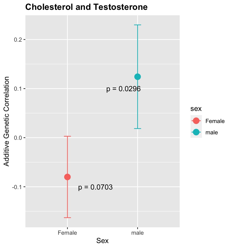
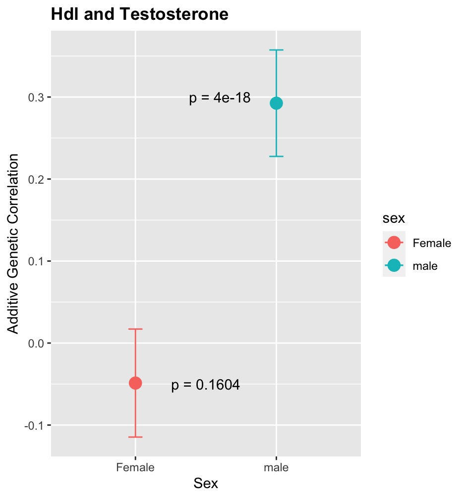
Figure 1: additive genetic correlation of Cholesterol and Testosterone, HDL and Testosterone(Sex-specific)

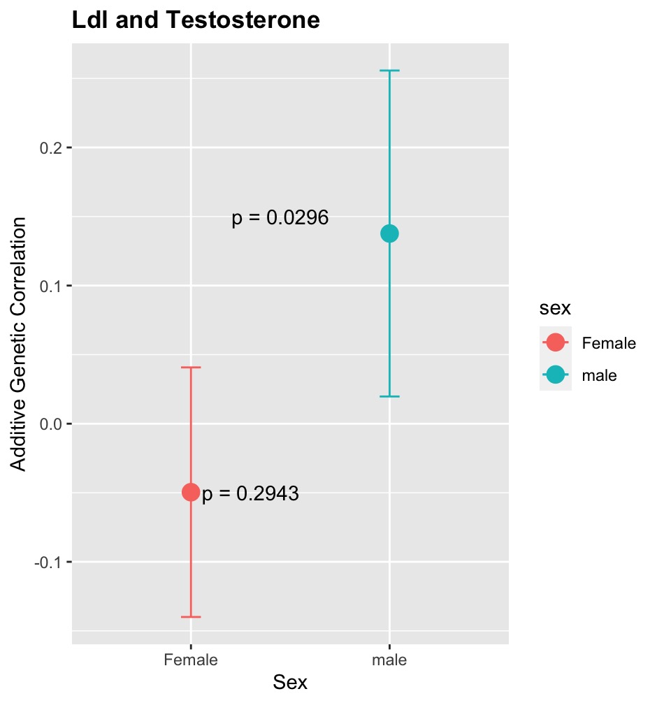
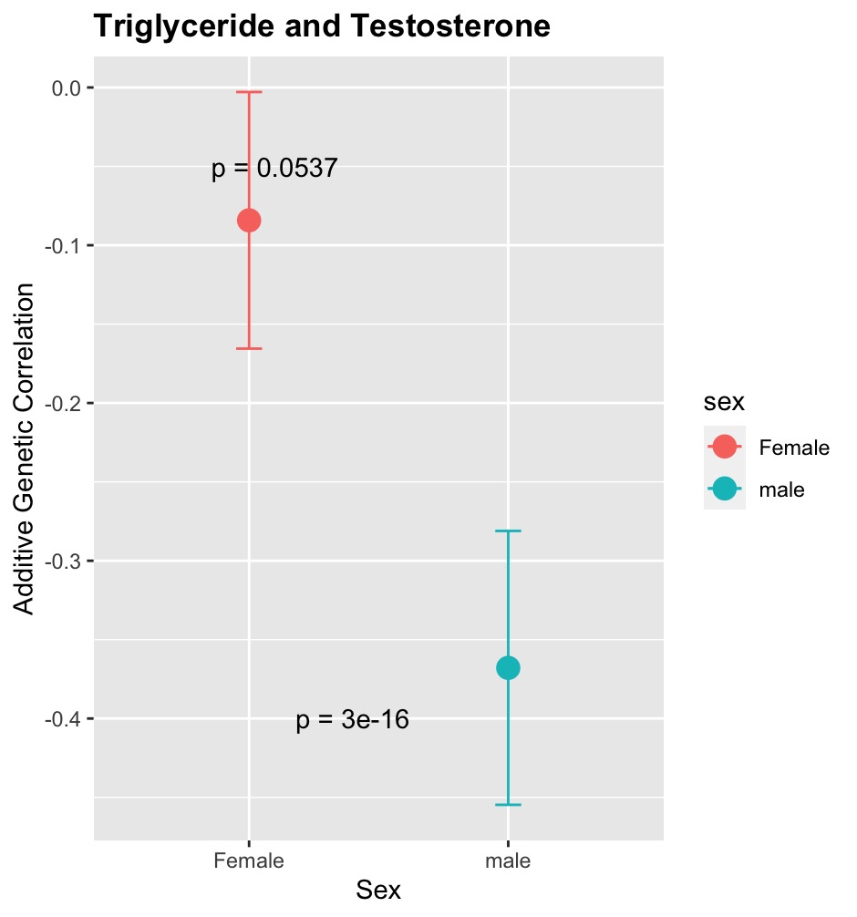
Figure 2: additive genetic correlation of LDL and Testosterone, Triglyceride and Testosterone (Sex-specific)

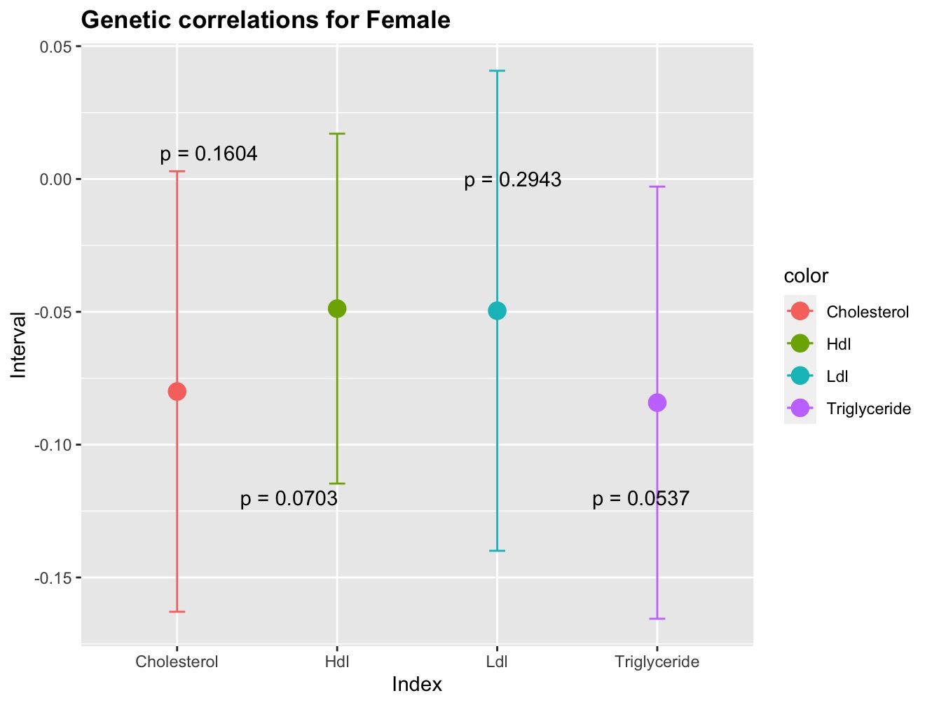
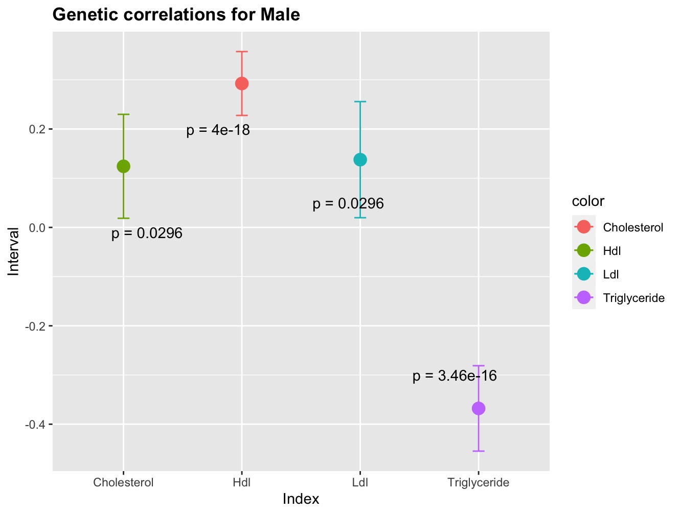
Figure 3: Additive genetic correlations for Males and Females

From Figure 1, we can see that for males, there is a positive additive genetic correlation between cholesterol and testosterone ($r_{g}=0.1242,p=0.0212$), i.e. with a significant amount of confidence against the null. This is also checked by the results of Gårevik et al. (2012), where they concluded that total cholesterol level was significantly increased by 15% two days after the testosterone injection (p = 0.007). The results are in concordance with that of Freedman et al. (1991), where they also acknowledged that levels of HDL cholesterol are positively associated with endogenous levels of testosterone in men, but they also made a cautious comment about the causality behind this correlation, but by additive genetic correlation study through LDSC, we confirm that the correlation of phenotypic effects of these by genetic variants across the genome on testosterone and cholesterol is significant and positive, i.e. due to genetic link between these, the correlation remains positive for males. Whereas for females we note the exact opposite thing, i.e., we see that the additive genetic correlation between these for females is negative with both confidence coefficients being negative. Also, we note an interesting thing in fig. 3 that the confidence intervals for males are way more shorter than females for each of the additive genetic correlation s. That is an indicator of the fact that due to a lower amount of testosterone being produced in females, the effects with the other phenotypes are not that much stronger as of males. That’s why we notice less evidence against the zero additive genetic correlation s as the p-value being $0.0586,0.147,0.282,0.04245$. Three of them are bigger than the standard $0.05$ norm and two are very close, while only one being less but not in a significant amount. That clearly indicates that for females, the additive genetic correlation s between testosterone with the others is not that much strong. On the other hand, we collect strong evidence against zero correlation for most of the cases for males, and with an almost nonzero correlation in each of the cases. That signifies the importance of the amount of testosterone to keep body hormones at their level very much. Leinonen et al. (2023) study shows that increasing testosterone in males overall promoted a favorable metabolic profile. It was positively correlated with HDL, cholesterol ($r_{g}>0.20,p<0.0011$), while negatively correlated with triglycerides ($r_{g}=-0.18,p=4.23-05$), that is concordant with our findings (Figure 1, 2, 3) using only the UK Biobank GWAS, whereas they used some other resources and constructed polygenic scores (PGS) for total testosterone, sex-hormone binding globulin (SHBG) and free testosterone. In contrast, they observed a negative correlation of HDL cholesterol with testosterone in females ($r_{g}=-0.18,p=4.2e-05$). But our study got the same results but at a lower significance level, that is for females, the linear correlation between those is not very significant, i.e. quite ambiguous. Ivanova et al. (2023) also obtained the same types of results for subjects in Russia. Testosterone is the most important circulating testicular androgen in men. Prospective cohort studies have shown that low serum testosterone levels are associated with a number of common disorders like cardiovascular disease (Vandenput and Ohlsson (2014)), which is caused by lipid profiles, though previous research are diverse in this context. According to Rubinow and Page (2012) even when reductions in HDL-cholesterol are observed as a consequence of androgen therapy, the implications for cardiovascular risk modification remain highly uncertain. whereas Laughlin, Barrett-Connor and Bergstrom (2008) claims that declining testosterone levels in elderly men are thought to underlie many of the symptoms and diseases of aging and Vikan et al. (2009) also consciously reported the results obtained by their research about this.

Trait1	Trait2	$r_{g}$	SE($r_{g}$)	CI($r_{g}$)	$\text{cov}_{g}$	SE($\text{cov}_{g}$)	CI($\text{cov}_{g}$)	p-value	$p_{\text{adjusted}}$
Triglyceride(Both)	Testosterone(Both)	-0.37	0.03	[-0.43, -0.30]	-0.04	0.01	[-0.24, -0.18]	0.00	0.00
Cholesterol(Both)	Testosterone(Both)	0.12	0.05	[0.03, 0.21]	0.01	0.00	[0.00, 0.05]	0.01	0.02
HDL(Both)	Testosterone(Both)	0.30	0.02	[0.26, 0.35]	0.04	0.00	[0.10, 0.13]	0.00	0.00
LDL(Both)	Testosterone(Both)	0.07	0.04	[-0.01, 0.15]	0.01	0.00	[0.01, 0.06]	0.11	0.12
HDL(Female)	Testosterone(Female)	-0.05	0.03	[-0.11, 0.02]	-0.01	0.00	[-0.02, 0.00]	0.15	0.16
Cholesterol(Female)	Testosterone(Female)	-0.08	0.04	[-0.16, 0.00]	-0.01	0.00	[0.00, 0.03]	0.06	0.07
LDL(Female)	Testosterone(Female)	-0.05	0.05	[-0.14, 0.04]	-0.00	0.00	[0.01, 0.03]	0.28	0.29
Triglyceride(Female)	Testosterone(Female)	-0.08	0.04	[-0.17, -0.00]	-0.01	0.01	[-0.02, 0.00]	0.04	0.05
Cholesterol(Female)	HDL(Female)	0.38	0.08	[0.23, 0.53]	0.06	0.01	[0.04, 0.08]	0.00	0.00
LDL(Female)	HDL(Female)	0.05	0.07	[-0.09, 0.18]	0.01	0.01	[-0.01, 0.02]	0.49	0.49
Triglyceride(Female)	HDL(Female)	-0.65	0.06	[-0.77, -0.53]	-0.13	0.02	[-0.17, -0.09]	0.00	0.00
Triglyceride(Female)	LDL(Female)	0.44	0.09	[0.27, 0.61]	0.06	0.01	[0.04, 0.08]	0.00	0.00
Cholesterol(Female)	LDL(Female)	0.94	0.01	[0.91, 0.96]	0.10	0.03	[0.05, 0.15]	0.00	0.00
Cholesterol(Female)	Triglyceride(Female)	0.28	0.07	[0.14, 0.42]	0.04	0.01	[0.02, 0.07]	0.00	0.00
Cholesterol(Male)	Testosterone(Male)	0.12	0.05	[0.02, 0.23]	0.02	0.01	[0.00, 0.03]	0.03	0.03
HDL(Male)	Testosterone(Male)	0.29	0.03	[0.23, 0.36]	0.05	0.01	[0.04, 0.06]	0.00	0.00
LDL(Male)	Testosterone(Male)	0.14	0.06	[0.02, 0.26]	0.01	0.01	[0.00, 0.03]	0.02	0.03
Triglyceride(Male)	Testosterone(Male)	-0.37	0.04	[-0.45, -0.28]	-0.07	0.01	[-0.08, -0.05]	0.00	0.00
Cholesterol(Male)	HDL(Male)	0.51	0.10	[0.31, 0.71]	0.07	0.01	[0.05, 0.09]	0.00	0.00
Triglyceride(Male)	HDL(Male)	-0.61	0.07	[-0.76, -0.47]	-0.12	0.03	[-0.17, -0.06]	0.00	0.00
LDL(Male)	HDL(Male)	0.34	0.11	[0.13, 0.56]	0.04	0.01	[0.02, 0.06]	0.00	0.00
Triglyceride(Male)	LDL(Male)	0.23	0.09	[0.05, 0.41]	0.03	0.01	[0.01, 0.04]	0.01	0.02
Cholesterol(Male)	LDL(Male)	0.96	0.01	[0.94, 0.98]	0.08	0.02	[0.03, 0.12]	0.00	0.00
Cholesterol(Male)	Triglyceride(Male)	0.25	0.10	[0.06, 0.44]	0.03	0.01	[0.01, 0.06]	0.01	0.02

Table 1: Additive Genetic Correlations and Covariances between the traits with respective Standard errors and 95$\%$ approximate confidence Intervals. ”$r_{g}$” represents the estimated additive genetic correlation, ”SE($r_{g}$)” is the estimated standard errors, ”CI” represents the 95$\%$ confidence interval, ”$\text{cov}_{g}$” represents estimated Genetic Covariance, ”SE($\text{cov}_{g}$)” denotes estimated standard error of the estimated genetic covariance and ”$p_{\text{adjusted}}$” denotes the adjusted p-value after multiple testing error.

Zhang et al. (2014) did a retrospective study on 11000 subjects to evaluate the relationship between serum total testosterone level and lipid profile after adjusting for some traditional confounding factors, free thyroid hormones and TSH in Chinese men, but they only included middle aged and elderly people (though, finally only 4114 male subjects from the general population were evaluated). In the bivariate correlation analysis, the correlation between Cholesterol and Testosterone was $r_{g}=-0.077,p=0.00$, between $logTG$ and Testosterone, $r_{g}=-0.374,p=0.00$, between LDL and Testosterone, $r_{g}=-0.069,p=0.00$. So, they didn’t get a strong correlation for LDL and Total Cholesterol. Firstly, this correlation was not purely genetic, also number of subjects was much much less in this study compared to our case, that can introduce a bias (also bias of age in their study) which can cause the amount of correlation significantly less. However, we got positive correlation of LDL, HDL and Total Cholesterol with Testosterone with a very significant p value ($\leq 0.03$) and less amount of SE, whereas significant negative correlation with Triglyceride which matches with that of Zhang et al. (2014). Also, Shamim et al. (2019) reported the correlations of Triglyceride ($p=0.0$), LDL ($p=0.5$), Cholesterol ($p=0.114$) with Teststerone were negative, and with HDL it was positive ($p=0.001$). However, the study was only on 200 people and results were highly non-significant. However none of these studies considered only the additive genetic correlations from their data, they only estimated the sample total correlation from the collected data.

Traits	$r_{g}$	SE($r_{g}$)	p-value	$cov_{g}$	SE($cov_{g}$)	$p_{adjusted}$
Testosterone	0.01	0.05	0.87	0.00	0.01	0.87
Cholesterol	0.85	0.04	0.00	0.09	0.02	0.00
LDL	0.81	0.06	0.00	0.07	0.02	0.00
HDL	0.91	0.02	0.00	0.18	0.03	0.00
Triglyceride	0.90	0.03	0.00	0.17	0.03	0.00

Table 2: Additive Genetic Correlation between Male and Female traits. ”$r_{g}$” means ”Estimated Additive Genetic Correlation”, ”SE” means estimated standard errors of the estimates, ”p” is the actual p-value and ”$p_{\text{adjusted}}$” is the adjusted p-value for multiple testing error. ”$cov_{g}$” means the estimated genetic covariance

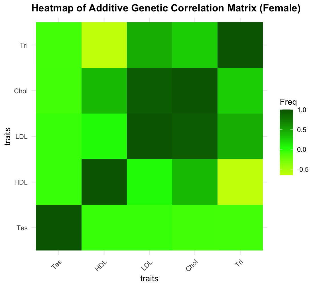
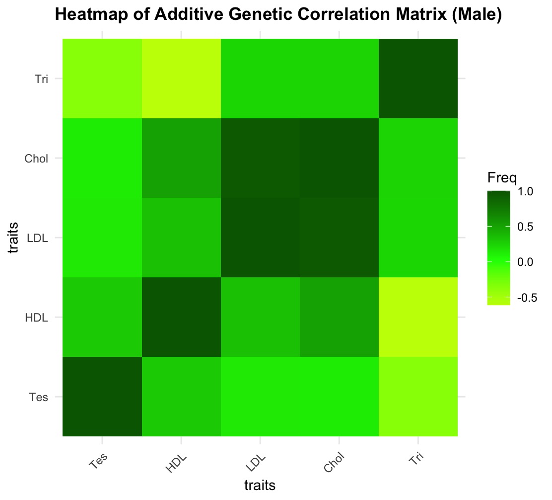
Figure 4: Heatmap for Estimated Additive Genetic Correlation matrix

Gender	Trait	$h(or,var_{g})$	SE($h(or,var_{g})$)	CI($h(or,var_{g})$)
M	Testosterone	0.17	0.02	[0.13, 0.21]
M	Triglyceride	0.18	0.04	[0.11, 0.25]
M	LDL	0.07	0.03	[0.01, 0.12]
M	HDL	0.20	0.03	[0.13, 0.27]
M	Cholesterol	0.09	0.02	[0.04, 0.14]
F	Testosterone	0.07	0.03	[0.01, 0.13]
F	Triglyceride	0.20	0.03	[0.14, 0.26]
F	LDL	0.09	0.03	[0.04, 0.15]
F	HDL	0.21	0.02	[0.16, 0.26]
F	Cholesterol	0.11	0.03	[0.06, 0.16]

Table 3: Heritibility of different traits, ”M” means Male, ”F” means Female. ”h” is the estimated scaled heritibility or genetic variance, ”hse” is the standard error of the estimate, CI is the approximate 95% Confidence Interval of the estimates

We observe from Table 3, the heritibilities of the selected lipid profiles and testosterone are ¡ 0.22 (with SE $\leqslant 0.4$). From Figure 4, the similarity between the additive genetic correlation matrix for males and females restricted to only lipid profile (i.e. HDL, LDL, Cholesterol, Triglycerides) is noteworthy. In particular, the additive genetic correlation matrices restricted to HDL, LDL, and Cholesterol have high similarity between males and females. Triglyceride levels and functioning changes during pregnancy time in Females(Ghio et al. (2011)). That can lead to significant difference in the distribution structures and sparsity of the underlying functioning of those.(Herrera et al. (2006)). Zhang et al. (2018) studied the triglyceride distributions for the people of North China. They performed a chi-squared test for the distributions of triglyceride sex wise and the distribution of triglyceride levels was different between males and females ($\chi^{2}=155.77,p<0.001$). Seidell et al. (1991) studied the sex effects of lipid profiles in European (The Netherlands, Sweden, Italy, and Poland) men and women, and their study concluded that fat distribution may be responsible for male/female differences in serum triglycerides but that such conclusions are less clear for HDL, total and LDL cholesterol. However, our study shows that the covariance variance structure for HDL, LDL and Cholesterol almost remains the same for females and males. The additive genetic variance–covariance matrix (G) summarizes the multivariate genetic relationships among a set of traits. So, we did a matrix comparison between females and males using Krzanowski’s common subspaces analysis (Aguirre et al. (2014), Chakrabarty and Schielzeth (2020)), Random Skewer’s Method (Cheverud and Marroig (2007), Aguirre et al. (2014)) and also using Bhattacharyya’s distance assuming gaussianity (Bhattacharyya (1943), Hennig (2010)). All of them lead to the same result, i.e., the distribution of the lipid profile concatenated with testosterone is similar for Males and Females. However, the amount of similarity increases when we remove the testosterone from the matrix. The shared space matrix is

$$\begin{bmatrix}0.19054899&0.2499404&-0.03439405&-0.02583797&-0.3068839\\ 0.24994042&1.1479944&0.31350653&0.52330668&-0.6512001\\ -0.03439405&0.3135065&0.62441997&0.73292240&0.4520197\\ -0.02583797&0.5233067&0.73292240&0.89170573&0.4072541\\ -0.30688389&-0.6512001&0.45201973&0.40725406&1.1453309\\ \end{bmatrix}$$

The largest two eigen values of the shared space matrix are 1.992132 and 1.896234. And, the corresponding eigen vectors are

$$\begin{bmatrix}0.05550021&-0.21930879\\ -0.26871768&-0.72488680\\ -0.55657367&-0.01659567\\ -0.65778482&-0.12427234\\ -0.42691382&0.64087733\\ \end{bmatrix}$$

PC1 vs PC2 plot for the variance-covariance matrices of males and females are in Figure 6. From Figure 6, we can see that the direction of maximum variance for males and females are very close to each other. However, a difference in Triglyceride and Testosterone are noted, which can be explained by the different functions of those in different sexes as described earlier. However, when testosterone is removed from the picture, the similarity between the directions of maximum explained variance even increases (Figure 7) and after removing triglycerides also, that direction almost becomes the same (Figure 7). That clearly indicates that except the complexities and functionalities created by Testosterone or Triglycerides in different sex, the lipid profiles of Males and Females matches very significantly. Keenly looking into Figure 7, we observe that the first maximum explainable direction is the most similar for all than the second. That means that most of the noises in the pattern of these traits in both the sexes is almost the same. Using Random Skewers Method (with seed 2023 in R), we get $r=0.9119407$ with $p=0.01$. After removing testosterone, $r=0.9698086$, $p=0.0$, and after removing triglyceride also, $r=0.9815491,p=0.0$. Using bhattacharrya’s distance under gaussianity assumption, the calculated measure for the whole matrix is 0.02, which is pretty small. So, using all the measures we can see that the underlying variance-covariance structure for the lipid profiles even with testerone is very much similar for males and females, and the similarity increases as we remove testosterone and triglyceride from the structure.

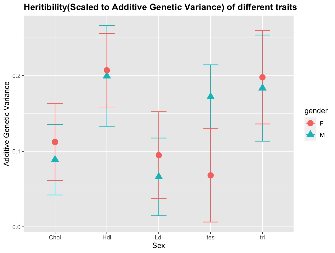
Figure 5: Heritibility of the traits

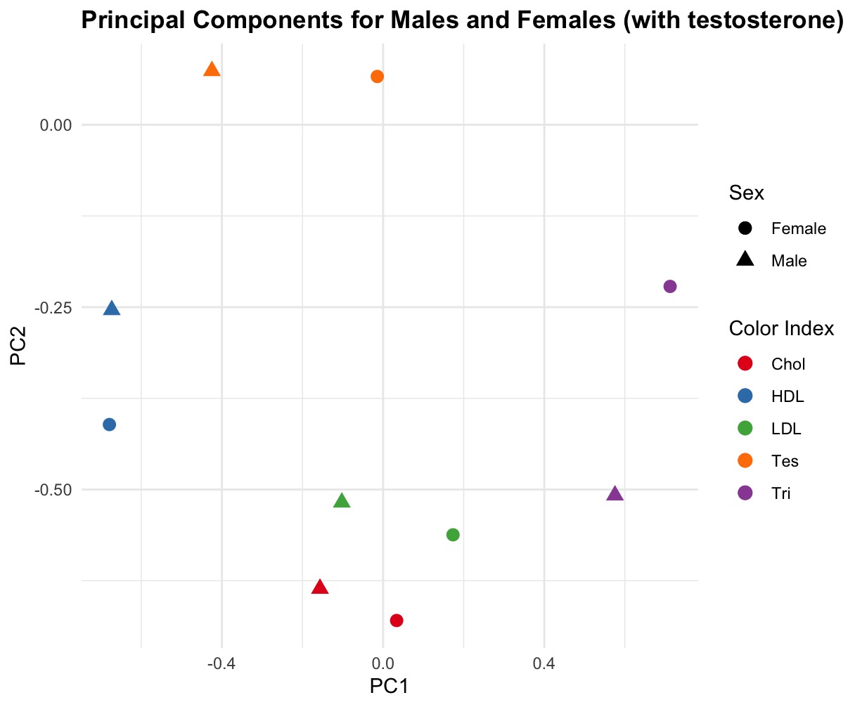
Figure 6: PC1 vs PC2 of the full variannce covariance matrix (including Testosterone)

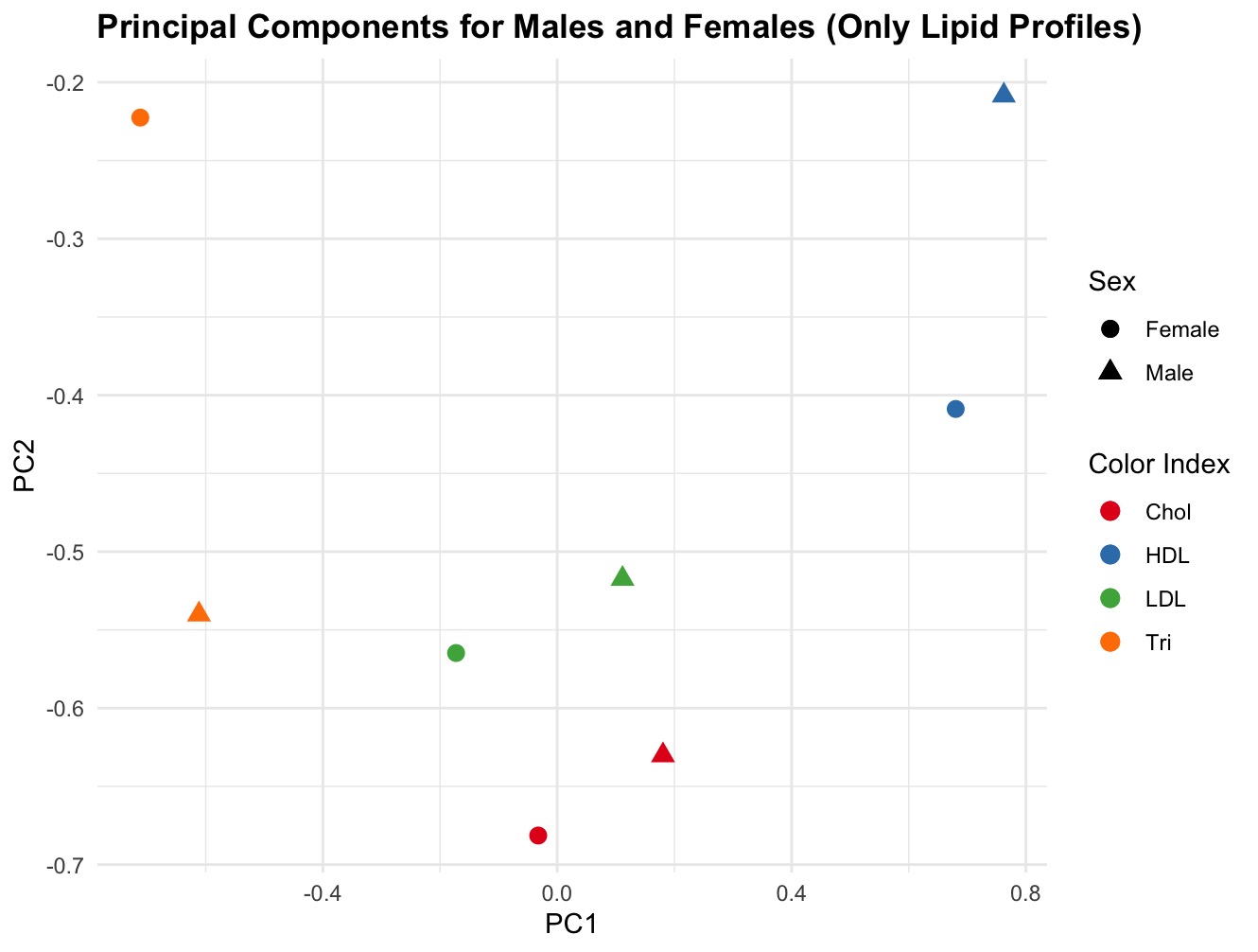
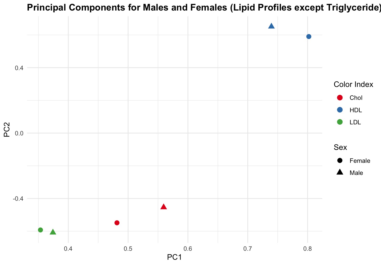
Figure 7: PC1 vs PC2 plot of the variance covariance matrix (first one, removing testosterone only and second one, removin triglyceride too)

4 Conclusions

Significant Positive and Negative correlations were found between testosterone and other lipid profiles for male, whereas for females the correlations are not much significant and almost close to 0. By the multivariate covariance matrix analysis, we confirm that for males and females, there is not much difference in the multivariate lipid profile structure.

5 Acknowledgements

The research conducted was graciously supported by the National Institute of Biomedical Genomics, Kalyani, India. We extend our sincere gratitude to our supervisors, Dr. Analabha Basu, Dr. Anasuya Chakrabarty, and Dr. Diptarup Nandi, for their invaluable guidance and support throughout this study. We would like to express a special acknowledgment to Dr. Anasuya Chakrabarty, whose guidance played a pivotal role in shaping the trajectory of our research. We are truly appreciative of her continuous involvement and insights.

References

- Aguirre et al. (2014) {barticle}[author] \bauthor\bsnmAguirre, \bfnmJD\binitsJ., \bauthor\bsnmHine, \bfnmE\binitsE., \bauthor\bsnmMcGuigan, \bfnmK\binitsK. and \bauthor\bsnmBlows, \bfnmMW\binitsM. (\byear2014). \btitleComparing G: multivariate analysis of genetic variation in multiple populations. \bjournalHeredity \bvolume112 \bpages21–29. \endbibitem
- Arnold and Phillips (1999) {barticle}[author] \bauthor\bsnmArnold, \bfnmStevan J\binitsS. J. and \bauthor\bsnmPhillips, \bfnmPatrick C\binitsP. C. (\byear1999). \btitleHIERARCHICAL COMPARISON OF GENETIC VARIANCE-COVARIANCE MATRICES. II COASTAL-INLAND DIVERGENCE IN THE GARTER SNAKE, THAMNOPHIS ELEGANS. \bjournalEvolution \bvolume53 \bpages1516–1527. \endbibitem
- Bégin and Roff (2001) {barticle}[author] \bauthor\bsnmBégin, \bfnmM\binitsM. and \bauthor\bsnmRoff, \bfnmDA\binitsD. (\byear2001). \btitleAn analysis of G matrix variation in two closely related cricket species, Gryllus firmus and G. pennsylvanicus. \bjournalJournal of Evolutionary Biology \bvolume14 \bpages1–13. \endbibitem
- Benjamini and Hochberg (1995) {barticle}[author] \bauthor\bsnmBenjamini, \bfnmYoav\binitsY. and \bauthor\bsnmHochberg, \bfnmYosef\binitsY. (\byear1995). \btitleControlling the false discovery rate: a practical and powerful approach to multiple testing. \bjournalJournal of the Royal statistical society: series B (Methodological) \bvolume57 \bpages289–300. \endbibitem
- Bhattacharyya (1943) {barticle}[author] \bauthor\bsnmBhattacharyya, \bfnmAnil\binitsA. (\byear1943). \btitleOn a measure of divergence between two statistical populations defined by their probability distribution. \bjournalBulletin of the Calcutta Mathematical Society \bvolume35 \bpages99–110. \endbibitem
- Brainstorm et al. (2018) {bmisc}[author] \bauthor\bsnmBrainstorm, \bfnmC\binitsC., \bauthor\bsnmAnttila, \bfnmV\binitsV., \bauthor\bsnmBulik-Sullivan, \bfnmB\binitsB., \bauthor\bsnmFinucane, \bfnmHK\binitsH., \bauthor\bsnmWalters, \bfnmRK\binitsR., \bauthor\bsnmBras, \bfnmJ\binitsJ., \bauthor\bsnmDuncan, \bfnmL\binitsL., \bauthor\bsnmEscott-Price, \bfnmV\binitsV., \bauthor\bsnmFalcone, \bfnmGJ\binitsG., \bauthor\bsnmGormley, \bfnmP\binitsP. \betalet al. (\byear2018). \btitleAnalysis of shared heritability in common disorders of the brain. Science. \endbibitem
- Bulik-Sullivan et al. (2015a) {barticle}[author] \bauthor\bsnmBulik-Sullivan, \bfnmBrendan K\binitsB. K., \bauthor\bsnmLoh, \bfnmPo-Ru\binitsP.-R., \bauthor\bsnmFinucane, \bfnmHilary K\binitsH. K., \bauthor\bsnmRipke, \bfnmStephan\binitsS., \bauthor\bsnmYang, \bfnmJian\binitsJ., \bauthor\bparticleof the \bsnmPsychiatric Genomics Consortium, \bfnmSchizophrenia Working Group\binitsS. W. G., \bauthor\bsnmPatterson, \bfnmNick\binitsN., \bauthor\bsnmDaly, \bfnmMark J\binitsM. J., \bauthor\bsnmPrice, \bfnmAlkes L\binitsA. L. and \bauthor\bsnmNeale, \bfnmBenjamin M\binitsB. M. (\byear2015a). \btitleLD Score regression distinguishes confounding from polygenicity in genome-wide association studies. \bjournalNature genetics \bvolume47 \bpages291–295. \endbibitem
- Bulik-Sullivan et al. (2015b) {barticle}[author] \bauthor\bsnmBulik-Sullivan, \bfnmBrendan\binitsB., \bauthor\bsnmFinucane, \bfnmHilary K\binitsH. K., \bauthor\bsnmAnttila, \bfnmVerneri\binitsV., \bauthor\bsnmGusev, \bfnmAlexander\binitsA., \bauthor\bsnmDay, \bfnmFelix R\binitsF. R., \bauthor\bsnmLoh, \bfnmPo-Ru\binitsP.-R., \bauthor\bsnmConsortium, \bfnmReproGen\binitsR., \bauthor\bsnmConsortium, \bfnmPsychiatric Genomics\binitsP. G., \bauthor\bparticlefor Anorexia Nervosa of the \bsnmWellcome Trust Case Control Consortium 3, \bfnmGenetic Consortium\binitsG. C., \bauthor\bsnmDuncan, \bfnmLaramie\binitsL. \betalet al. (\byear2015b). \btitleAn atlas of genetic correlations across human diseases and traits. \bjournalNature genetics \bvolume47 \bpages1236–1241. \endbibitem
- Chakrabarty and Schielzeth (2020) {barticle}[author] \bauthor\bsnmChakrabarty, \bfnmAnasuya\binitsA. and \bauthor\bsnmSchielzeth, \bfnmHolger\binitsH. (\byear2020). \btitleComparative analysis of the multivariate genetic architecture of morphological traits in three species of Gomphocerine grasshoppers. \bjournalHeredity \bvolume124 \bpages367–382. \endbibitem
- Cheverud (1996) {barticle}[author] \bauthor\bsnmCheverud, \bfnmJames M\binitsJ. M. (\byear1996). \btitleQuantitative genetic analysis of cranial morphology in the cotton-top (Saguinus oedipus) and saddle-back (S. fuscicollis) tamarins. \bjournalJournal of Evolutionary Biology \bvolume9 \bpages5–42. \endbibitem
- Cheverud and Marroig (2007) {barticle}[author] \bauthor\bsnmCheverud, \bfnmJames M\binitsJ. M. and \bauthor\bsnmMarroig, \bfnmGabriel\binitsG. (\byear2007). \btitleResearch article comparing covariance matrices: random skewers method compared to the common principal components model. \bjournalGenetics and Molecular Biology \bvolume30 \bpages461–469. \endbibitem
- Falconer (1996) {bbook}[author] \bauthor\bsnmFalconer, \bfnmDouglas Scott\binitsD. S. (\byear1996). \btitleIntroduction to quantitative genetics. \bpublisherPearson Education India. \endbibitem
- Flury (1988) {bbook}[author] \bauthor\bsnmFlury, \bfnmBernhard\binitsB. (\byear1988). \btitleCommon principal components & related multivariate models. \bpublisherJohn Wiley & Sons, Inc. \endbibitem
- Freedman et al. (1991) {barticle}[author] \bauthor\bsnmFreedman, \bfnmDavid S\binitsD. S., \bauthor\bsnmO’Brien, \bfnmThomas R\binitsT. R., \bauthor\bsnmFlanders, \bfnmW Dana\binitsW. D., \bauthor\bsnmDeStefano, \bfnmFrank\binitsF. and \bauthor\bsnmBarboriak, \bfnmJoseph J\binitsJ. J. (\byear1991). \btitleRelation of serum testosterone levels to high density lipoprotein cholesterol and other characteristics in men. \bjournalArteriosclerosis and thrombosis: a journal of vascular biology \bvolume11 \bpages307–315. \endbibitem
- Gårevik et al. (2012) {barticle}[author] \bauthor\bsnmGårevik, \bfnmNina\binitsN., \bauthor\bsnmSkogastierna, \bfnmCristine\binitsC., \bauthor\bsnmRane, \bfnmAnders\binitsA. and \bauthor\bsnmEkström, \bfnmLena\binitsL. (\byear2012). \btitleSingle dose testosterone increases total cholesterol levels and induces the expression of HMG CoA Reductase. \bjournalSubstance abuse treatment, prevention, and policy \bvolume7 \bpages1–6. \endbibitem
- Ghio et al. (2011) {barticle}[author] \bauthor\bsnmGhio, \bfnmAlessandra\binitsA., \bauthor\bsnmBertolotto, \bfnmAlessandra\binitsA., \bauthor\bsnmResi, \bfnmVeronica\binitsV., \bauthor\bsnmVolpe, \bfnmLaura\binitsL. and \bauthor\bsnmDi Cianni, \bfnmGraziano\binitsG. (\byear2011). \btitleTriglyceride metabolism in pregnancy. \bjournalAdvances in clinical chemistry \bvolume55 \bpages134. \endbibitem
- Gosden and Chenoweth (2014) {barticle}[author] \bauthor\bsnmGosden, \bfnmThomas P\binitsT. P. and \bauthor\bsnmChenoweth, \bfnmStephen F\binitsS. F. (\byear2014). \btitleThe evolutionary stability of cross-sex, cross-trait genetic covariances. \bjournalEvolution \bvolume68 \bpages1687–1697. \endbibitem
- Grüneberg (1938) {barticle}[author] \bauthor\bsnmGrüneberg, \bfnmHans\binitsH. (\byear1938). \btitleAn analysis of the “pleiotropic” effects of a new lethal mutation in the rat (Mus norvegicus). \bjournalProceedings of the Royal Society of London. Series B-Biological Sciences \bvolume125 \bpages123–144. \endbibitem
- Hackinger and Zeggini (2017) {barticle}[author] \bauthor\bsnmHackinger, \bfnmSophie\binitsS. and \bauthor\bsnmZeggini, \bfnmEleftheria\binitsE. (\byear2017). \btitleStatistical methods to detect pleiotropy in human complex traits. \bjournalOpen biology \bvolume7 \bpages170125. \endbibitem
- Hennig (2010) {barticle}[author] \bauthor\bsnmHennig, \bfnmChristian\binitsC. (\byear2010). \btitleMethods for merging Gaussian mixture components. \bjournalAdvances in data analysis and classification \bvolume4 \bpages3–34. \endbibitem
- Hennig and Imports (2015) {barticle}[author] \bauthor\bsnmHennig, \bfnmChristian\binitsC. and \bauthor\bsnmImports, \bfnmMASS\binitsM. (\byear2015). \btitlePackage ‘fpc’. \bjournalFlexible Procedures for Clustering \bvolume1176. \endbibitem
- Herrera et al. (2006) {barticle}[author] \bauthor\bsnmHerrera, \bfnmE\binitsE., \bauthor\bsnmAmusquivar, \bfnmE\binitsE., \bauthor\bsnmLopez-Soldado, \bfnmI\binitsI. and \bauthor\bsnmOrtega, \bfnmH\binitsH. (\byear2006). \btitleMaternal lipid metabolism and placental lipid transfer. \bjournalHormone Research in Paediatrics \bvolume65 \bpages59–64. \endbibitem
- Holm (1979) {barticle}[author] \bauthor\bsnmHolm, \bfnmSture\binitsS. (\byear1979). \btitleA simple sequentially rejective multiple test procedure. \bjournalScandinavian journal of statistics \bpages65–70. \endbibitem
- Ivanova et al. (2023) {barticle}[author] \bauthor\bsnmIvanova, \bfnmTatiana\binitsT., \bauthor\bsnmChurnosova, \bfnmMaria\binitsM., \bauthor\bsnmAbramova, \bfnmMaria\binitsM., \bauthor\bsnmPlotnikov, \bfnmDenis\binitsD., \bauthor\bsnmPonomarenko, \bfnmIrina\binitsI., \bauthor\bsnmReshetnikov, \bfnmEvgeny\binitsE., \bauthor\bsnmAristova, \bfnmInna\binitsI., \bauthor\bsnmSorokina, \bfnmInna\binitsI. and \bauthor\bsnmChurnosov, \bfnmMikhail\binitsM. (\byear2023). \btitleSex-Specific Features of the Correlation between GWAS-Noticeable Polymorphisms and Hypertension in Europeans of Russia. \bjournalInternational Journal of Molecular Sciences \bvolume24 \bpages7799. \endbibitem
- Jansen et al. (2019) {barticle}[author] \bauthor\bsnmJansen, \bfnmPhilip R\binitsP. R., \bauthor\bsnmWatanabe, \bfnmKyoko\binitsK., \bauthor\bsnmStringer, \bfnmSven\binitsS., \bauthor\bsnmSkene, \bfnmNathan\binitsN., \bauthor\bsnmBryois, \bfnmJulien\binitsJ., \bauthor\bsnmHammerschlag, \bfnmAnke R\binitsA. R., \bauthor\bparticlede \bsnmLeeuw, \bfnmChristiaan A\binitsC. A., \bauthor\bsnmBenjamins, \bfnmJeroen S\binitsJ. S., \bauthor\bsnmMuñoz-Manchado, \bfnmAna B\binitsA. B., \bauthor\bsnmNagel, \bfnmMats\binitsM. \betalet al. (\byear2019). \btitleGenome-wide analysis of insomnia in 1,331,010 individuals identifies new risk loci and functional pathways. \bjournalNature genetics \bvolume51 \bpages394–403. \endbibitem
- Krzanowski (1979) {barticle}[author] \bauthor\bsnmKrzanowski, \bfnmWJ\binitsW. (\byear1979). \btitleBetween-groups comparison of principal components. \bjournalJournal of the american statistical association \bvolume74 \bpages703–707. \endbibitem
- Lande (1979) {barticle}[author] \bauthor\bsnmLande, \bfnmRussell\binitsR. (\byear1979). \btitleQuantitative genetic analysis of multivariate evolution, applied to brain: body size allometry. \bjournalEvolution \bpages402–416. \endbibitem
- Laughlin, Barrett-Connor and Bergstrom (2008) {barticle}[author] \bauthor\bsnmLaughlin, \bfnmGail A\binitsG. A., \bauthor\bsnmBarrett-Connor, \bfnmElizabeth\binitsE. and \bauthor\bsnmBergstrom, \bfnmJaclyn\binitsJ. (\byear2008). \btitleLow serum testosterone and mortality in older men. \bjournalThe Journal of Clinical Endocrinology & Metabolism \bvolume93 \bpages68–75. \endbibitem
- Lee et al. (2018) {barticle}[author] \bauthor\bsnmLee, \bfnmJames J\binitsJ. J., \bauthor\bsnmWedow, \bfnmRobbee\binitsR., \bauthor\bsnmOkbay, \bfnmAysu\binitsA., \bauthor\bsnmKong, \bfnmEdward\binitsE., \bauthor\bsnmMaghzian, \bfnmOmeed\binitsO., \bauthor\bsnmZacher, \bfnmMeghan\binitsM., \bauthor\bsnmNguyen-Viet, \bfnmTuan Anh\binitsT. A., \bauthor\bsnmBowers, \bfnmPeter\binitsP., \bauthor\bsnmSidorenko, \bfnmJulia\binitsJ., \bauthor\bsnmKarlsson Linnér, \bfnmRichard\binitsR. \betalet al. (\byear2018). \btitleGene discovery and polygenic prediction from a genome-wide association study of educational attainment in 1.1 million individuals. \bjournalNature genetics \bvolume50 \bpages1112–1121. \endbibitem
- Leinonen et al. (2023) {barticle}[author] \bauthor\bsnmLeinonen, \bfnmJaakko T\binitsJ. T., \bauthor\bsnmMars, \bfnmNina\binitsN., \bauthor\bsnmLehtonen, \bfnmLeevi E\binitsL. E., \bauthor\bsnmAhola-Olli, \bfnmAri\binitsA., \bauthor\bsnmRuotsalainen, \bfnmSanni\binitsS., \bauthor\bsnmLehtimäki, \bfnmTerho\binitsT., \bauthor\bsnmKähönen, \bfnmMika\binitsM., \bauthor\bsnmRaitakari, \bfnmOlli\binitsO., \bauthor\bsnm17, \bfnmFinnGen Consortium Mars Nina 17 Ruotsalainen Sanni 17 Kähönen Mika 5 18 Piltonen Terhi 19 Tuomi Tiinamaija 17 20 21 22 23 Daly Mark 17 24 Ripatti Samuli 17 24 25 Tukiainen Taru\binitsF. C. M. N. . R. S. . K. M. . . P. T. . T. T. . . . . . D. M. . . R. S. . . . T. T., \bauthor\bsnmPiltonen, \bfnmTerhi\binitsT. \betalet al. (\byear2023). \btitleGenetic analyses implicate complex links between adult testosterone levels and health and disease. \bjournalCommunications Medicine \bvolume3 \bpages4. \endbibitem
- Loh et al. (2018) {barticle}[author] \bauthor\bsnmLoh, \bfnmPo-Ru\binitsP.-R., \bauthor\bsnmKichaev, \bfnmGleb\binitsG., \bauthor\bsnmGazal, \bfnmSteven\binitsS., \bauthor\bsnmSchoech, \bfnmArmin P\binitsA. P. and \bauthor\bsnmPrice, \bfnmAlkes L\binitsA. L. (\byear2018). \btitleMixed-model association for biobank-scale datasets. \bjournalNature genetics \bvolume50 \bpages906–908. \endbibitem
- Lynch et al. (1998) {bbook}[author] \bauthor\bsnmLynch, \bfnmMichael\binitsM., \bauthor\bsnmWalsh, \bfnmBruce\binitsB. \betalet al. (\byear1998). \btitleGenetics and analysis of quantitative traits \bvolume1. \bpublisherSinauer Sunderland, MA. \endbibitem
- Maes (2000) {bmisc}[author] \bauthor\bsnmMaes, \bfnmMichael C Neale Hermine HM\binitsM. C. N. H. H. (\byear2000). \btitleMethodology for Genetic Studies of Twins and Families. \endbibitem
- Melo et al. (2015) {barticle}[author] \bauthor\bsnmMelo, \bfnmDiogo\binitsD., \bauthor\bsnmGarcia, \bfnmGuilherme\binitsG., \bauthor\bsnmHubbe, \bfnmAlex\binitsA., \bauthor\bsnmAssis, \bfnmAna Paula\binitsA. P. and \bauthor\bsnmMarroig, \bfnmGabriel\binitsG. (\byear2015). \btitleEvolQG-An R package for evolutionary quantitative genetics. \bjournalF1000Research \bvolume4. \endbibitem
- Phillips and Arnold (1999) {barticle}[author] \bauthor\bsnmPhillips, \bfnmPatrick C\binitsP. C. and \bauthor\bsnmArnold, \bfnmStevan J\binitsS. J. (\byear1999). \btitleHierarchical comparison of genetic variance-covariance matrices. I. Using the Flury hierarchy. \bjournalEvolution \bvolume53 \bpages1506–1515. \endbibitem
- Revell (2012) {barticle}[author] \bauthor\bsnmRevell, \bfnmLiam J\binitsL. J. (\byear2012). \btitlephytools: an R package for phylogenetic comparative biology (and other things). \bjournalMethods in ecology and evolution \bvolume2 \bpages217–223. \endbibitem
- Roff (2000) {barticle}[author] \bauthor\bsnmRoff (\byear2000). \btitleTrade-offs between growth and reproduction: an analysis of the quantitative genetic evidence. \bjournalJournal of Evolutionary Biology \bvolume13 \bpages434–445. \endbibitem
- Roff et al. (2012) {barticle}[author] \bauthor\bsnmRoff, \bfnmDA\binitsD., \bauthor\bsnmProkkola, \bfnmJM\binitsJ., \bauthor\bsnmKrams, \bfnmI\binitsI. and \bauthor\bsnmRantala, \bfnmMJ\binitsM. (\byear2012). \btitleThere is more than one way to skin a G matrix. \bjournalJournal of evolutionary biology \bvolume25 \bpages1113–1126. \endbibitem
- Rubinow and Page (2012) {bmisc}[author] \bauthor\bsnmRubinow, \bfnmKatya B\binitsK. B. and \bauthor\bsnmPage, \bfnmStephanie T\binitsS. T. (\byear2012). \btitleTestosterone, HDL and cardiovascular risk in men: the jury is still out. \endbibitem
- Seidell et al. (1991) {barticle}[author] \bauthor\bsnmSeidell, \bfnmJacob C\binitsJ. C., \bauthor\bsnmCigolini, \bfnmMassimo\binitsM., \bauthor\bsnmCharzewska, \bfnmJadviga\binitsJ., \bauthor\bsnmEllsinger, \bfnmBritt-Marie\binitsB.-M., \bauthor\bsnmBjörntorp, \bfnmPer\binitsP., \bauthor\bsnmHautvast, \bfnmJoseph GAJ\binitsJ. G. and \bauthor\bsnmSzostak, \bfnmWictor\binitsW. (\byear1991). \btitleFat distribution and gender differences in serum lipids in men and women from four European communities. \bjournalAtherosclerosis \bvolume87 \bpages203–210. \endbibitem
- Shamim et al. (2019) {barticle}[author] \bauthor\bsnmShamim, \bfnmMuhammad Omar\binitsM. O., \bauthor\bsnmKhan, \bfnmFarooq Munfaet Ali\binitsF. M. A., \bauthor\bsnmGill, \bfnmMaria\binitsM., \bauthor\bsnmRasheed, \bfnmAaqiba\binitsA. and \bauthor\bsnmMahmood, \bfnmAtif\binitsA. (\byear2019). \btitleAffiliation of Serum Total Testosterone with Lipid profile in Healthy Middle Aged Males. \bjournalNational Editorial Advisory Board \bvolume30. \endbibitem
- Shaw et al. (1995) {barticle}[author] \bauthor\bsnmShaw, \bfnmFrank H\binitsF. H., \bauthor\bsnmShaw, \bfnmRuth G\binitsR. G., \bauthor\bsnmWilkinson, \bfnmGerald S\binitsG. S. and \bauthor\bsnmTurelli, \bfnmMichael\binitsM. (\byear1995). \btitleChanges in genetic variances and covariances: G whiz! \bjournalEvolution \bpages1260–1267. \endbibitem
- Solovieff et al. (2013) {barticle}[author] \bauthor\bsnmSolovieff, \bfnmNadia\binitsN., \bauthor\bsnmCotsapas, \bfnmChris\binitsC., \bauthor\bsnmLee, \bfnmPhil H\binitsP. H., \bauthor\bsnmPurcell, \bfnmShaun M\binitsS. M. and \bauthor\bsnmSmoller, \bfnmJordan W\binitsJ. W. (\byear2013). \btitlePleiotropy in complex traits: challenges and strategies. \bjournalNature Reviews Genetics \bvolume14 \bpages483–495. \endbibitem
- Stearns (2010) {barticle}[author] \bauthor\bsnmStearns, \bfnmFrank W\binitsF. W. (\byear2010). \btitleOne hundred years of pleiotropy: a retrospective. \bjournalGenetics \bvolume186 \bpages767–773. \endbibitem
- Steppan, Phillips and Houle (2002) {barticle}[author] \bauthor\bsnmSteppan, \bfnmScott J\binitsS. J., \bauthor\bsnmPhillips, \bfnmPatrick C\binitsP. C. and \bauthor\bsnmHoule, \bfnmDavid\binitsD. (\byear2002). \btitleComparative quantitative genetics: evolution of the G matrix. \bjournalTrends in ecology & evolution \bvolume17 \bpages320–327. \endbibitem
- Uffelmann et al. (2021) {barticle}[author] \bauthor\bsnmUffelmann, \bfnmEmil\binitsE., \bauthor\bsnmHuang, \bfnmQin Qin\binitsQ. Q., \bauthor\bsnmMunung, \bfnmNchangwi Syntia\binitsN. S., \bauthor\bsnmDe Vries, \bfnmJantina\binitsJ., \bauthor\bsnmOkada, \bfnmYukinori\binitsY., \bauthor\bsnmMartin, \bfnmAlicia R\binitsA. R., \bauthor\bsnmMartin, \bfnmHilary C\binitsH. C., \bauthor\bsnmLappalainen, \bfnmTuuli\binitsT. and \bauthor\bsnmPosthuma, \bfnmDanielle\binitsD. (\byear2021). \btitleGenome-wide association studies. \bjournalNature Reviews Methods Primers \bvolume1 \bpages59. \endbibitem
- Van Rheenen et al. (2019) {barticle}[author] \bauthor\bsnmVan Rheenen, \bfnmWouter\binitsW., \bauthor\bsnmPeyrot, \bfnmWouter J\binitsW. J., \bauthor\bsnmSchork, \bfnmAndrew J\binitsA. J., \bauthor\bsnmLee, \bfnmS Hong\binitsS. H. and \bauthor\bsnmWray, \bfnmNaomi R\binitsN. R. (\byear2019). \btitleGenetic correlations of polygenic disease traits: from theory to practice. \bjournalNature Reviews Genetics \bvolume20 \bpages567–581. \endbibitem
- Vandenput and Ohlsson (2014) {barticle}[author] \bauthor\bsnmVandenput, \bfnmLiesbeth\binitsL. and \bauthor\bsnmOhlsson, \bfnmClaes\binitsC. (\byear2014). \btitleGenome-wide association studies on serum sex steroid levels. \bjournalMolecular and Cellular Endocrinology \bvolume382 \bpages758–766. \endbibitem
- Verbanck et al. (2018) {barticle}[author] \bauthor\bsnmVerbanck, \bfnmMarie\binitsM., \bauthor\bsnmChen, \bfnmChia-Yen\binitsC.-Y., \bauthor\bsnmNeale, \bfnmBenjamin\binitsB. and \bauthor\bsnmDo, \bfnmRon\binitsR. (\byear2018). \btitleDetection of widespread horizontal pleiotropy in causal relationships inferred from Mendelian randomization between complex traits and diseases. \bjournalNature genetics \bvolume50 \bpages693–698. \endbibitem
- Vikan et al. (2009) {barticle}[author] \bauthor\bsnmVikan, \bfnmT\binitsT., \bauthor\bsnmJohnsen, \bfnmSH\binitsS., \bauthor\bsnmSchirmer, \bfnmH\binitsH., \bauthor\bsnmNjølstad, \bfnmI\binitsI. and \bauthor\bsnmSvartberg, \bfnmJ\binitsJ. (\byear2009). \btitleEndogenous testosterone and the prospective association with carotid atherosclerosis in men: the Tromsø study. \bjournalEuropean journal of epidemiology \bvolume24 \bpages289–295. \endbibitem
- Wagner and Zhang (2011) {barticle}[author] \bauthor\bsnmWagner, \bfnmGünter P\binitsG. P. and \bauthor\bsnmZhang, \bfnmJianzhi\binitsJ. (\byear2011). \btitleThe pleiotropic structure of the genotype–phenotype map: the evolvability of complex organisms. \bjournalNature Reviews Genetics \bvolume12 \bpages204–213. \endbibitem
- (52) {barticle}[author] \bauthor\bsnmWarrington, \bfnmHilary K\binitsH. K., \bauthor\bsnmPrice, \bfnmAlkes L\binitsA. L., \bauthor\bsnmBulik-Sullivan, \bfnmBrendan K\binitsB. K., \bauthor\bsnmAnttila, \bfnmVerneri\binitsV., \bauthor\bsnmPaternoster, \bfnmLavinia\binitsL., \bauthor\bsnmGaunt, \bfnmTom R\binitsT. R., \bauthor\bsnmEvans, \bfnmDavid M\binitsD. M. and \bauthor\bsnmNeale, \bfnmBenjamin M\binitsB. M. \btitleLD Hub: a centralized database and web interface to perform LD score regression that maximizes the potential of summary level GWAS data for SNP heritability and genetic correlation analysis. \endbibitem
- Watanabe et al. (2019) {barticle}[author] \bauthor\bsnmWatanabe, \bfnmKyoko\binitsK., \bauthor\bsnmStringer, \bfnmSven\binitsS., \bauthor\bsnmFrei, \bfnmOleksandr\binitsO., \bauthor\bsnmUmićević Mirkov, \bfnmMaša\binitsM., \bauthor\bparticlede \bsnmLeeuw, \bfnmChristiaan\binitsC., \bauthor\bsnmPolderman, \bfnmTinca JC\binitsT. J., \bauthor\bparticlevan der \bsnmSluis, \bfnmSophie\binitsS., \bauthor\bsnmAndreassen, \bfnmOle A\binitsO. A., \bauthor\bsnmNeale, \bfnmBenjamin M\binitsB. M. and \bauthor\bsnmPosthuma, \bfnmDanielle\binitsD. (\byear2019). \btitleA global overview of pleiotropy and genetic architecture in complex traits. \bjournalNature genetics \bvolume51 \bpages1339–1348. \endbibitem
- Zhang et al. (2014) {barticle}[author] \bauthor\bsnmZhang, \bfnmNan\binitsN., \bauthor\bsnmZhang, \bfnmHaiqing\binitsH., \bauthor\bsnmZhang, \bfnmXU\binitsX., \bauthor\bsnmZhang, \bfnmBingchang\binitsB., \bauthor\bsnmWang, \bfnmFurong\binitsF., \bauthor\bsnmWang, \bfnmChenggang\binitsC., \bauthor\bsnmZhao, \bfnmMeng\binitsM., \bauthor\bsnmYu, \bfnmChunxiao\binitsC., \bauthor\bsnmGao, \bfnmLing\binitsL., \bauthor\bsnmZhao, \bfnmJiajun\binitsJ. \betalet al. (\byear2014). \btitleThe relationship between endogenous testosterone and lipid profile in middle-aged and elderly Chinese men. \bjournalEuropean journal of endocrinology \bvolume170 \bpages487–494. \endbibitem
- Zhang et al. (2018) {barticle}[author] \bauthor\bsnmZhang, \bfnmAnning\binitsA., \bauthor\bsnmYao, \bfnmYan\binitsY., \bauthor\bsnmXue, \bfnmZhiqiang\binitsZ., \bauthor\bsnmGuo, \bfnmXin\binitsX., \bauthor\bsnmDou, \bfnmJing\binitsJ., \bauthor\bsnmLv, \bfnmYaogai\binitsY., \bauthor\bsnmShen, \bfnmLi\binitsL., \bauthor\bsnmYu, \bfnmYaqin\binitsY. and \bauthor\bsnmJin, \bfnmLina\binitsL. (\byear2018). \btitleA study on the factors influencing triglyceride levels among adults in Northeast China. \bjournalScientific reports \bvolume8 \bpages6388. \endbibitem
- Zheng et al. (2016) {barticle}[author] \bauthor\bsnmZheng, \bfnmJie\binitsJ., \bauthor\bsnmErzurumluoglu, \bfnmA Mesut\binitsA. M., \bauthor\bsnmElsworth, \bfnmBenjamin L\binitsB. L., \bauthor\bsnmKemp, \bfnmJohn P\binitsJ. P., \bauthor\bsnmHowe, \bfnmLaurence\binitsL., \bauthor\bsnmHaycock, \bfnmPhilip C\binitsP. C., \bauthor\bsnmHemani, \bfnmGibran\binitsG., \bauthor\bsnmTansey, \bfnmKatherine\binitsK., \bauthor\bsnmLaurin, \bfnmCharles\binitsC., \bauthor\bsnmGenetics, \bfnmEarly\binitsE., \bauthor\bsnmConsortium, \bfnmLifecourse Epidemiology (EAGLE) Eczema\binitsL. E. E. E., \bauthor\bsnmPourcain, \bfnmBeate St\binitsB. S., \bauthor\bsnmWarrington, \bfnmNicole M\binitsN. M., \bauthor\bsnmFinucane, \bfnmHilary K\binitsH. K., \bauthor\bsnmPrice, \bfnmAlkes L\binitsA. L., \bauthor\bsnmBulik-Sullivan, \bfnmBrendan K\binitsB. K., \bauthor\bsnmAnttila, \bfnmVerneri\binitsV., \bauthor\bsnmPaternoster, \bfnmLavinia\binitsL., \bauthor\bsnmGaunt, \bfnmTom R\binitsT. R., \bauthor\bsnmEvans, \bfnmDavid M\binitsD. M. and \bauthor\bsnmNeale, \bfnmBenjamin M\binitsB. M. (\byear2016). \btitleLD Hub: a centralized database and web interface to perform LD score regression that maximizes the potential of summary level GWAS data for SNP heritability and genetic correlation analysis. \bjournalBioinformatics \bvolume33 \bpages272-279. \bdoi10.1093/bioinformatics/btw613 \endbibitem
- Zhu et al. (2018) {barticle}[author] \bauthor\bsnmZhu, \bfnmZhihong\binitsZ., \bauthor\bsnmZheng, \bfnmZhili\binitsZ., \bauthor\bsnmZhang, \bfnmFutao\binitsF., \bauthor\bsnmWu, \bfnmYang\binitsY., \bauthor\bsnmTrzaskowski, \bfnmMaciej\binitsM., \bauthor\bsnmMaier, \bfnmRobert\binitsR., \bauthor\bsnmRobinson, \bfnmMatthew R\binitsM. R., \bauthor\bsnmMcGrath, \bfnmJohn J\binitsJ. J., \bauthor\bsnmVisscher, \bfnmPeter M\binitsP. M., \bauthor\bsnmWray, \bfnmNaomi R\binitsN. R. \betalet al. (\byear2018). \btitleCausal associations between risk factors and common diseases inferred from GWAS summary data. \bjournalNature communications \bvolume9 \bpages1–12. \endbibitem
- Zuk et al. (2012) {barticle}[author] \bauthor\bsnmZuk, \bfnmOr\binitsO., \bauthor\bsnmHechter, \bfnmEliana\binitsE., \bauthor\bsnmSunyaev, \bfnmShamil R\binitsS. R. and \bauthor\bsnmLander, \bfnmEric S\binitsE. S. (\byear2012). \btitleThe mystery of missing heritability: Genetic interactions create phantom heritability. \bjournalProceedings of the National Academy of Sciences \bvolume109 \bpages1193–1198. \endbibitem