Superradiant stability of the Kerr black hole

Abstract

We know that Kerr black holes are stable for specific conditions.In this article, we use algebraic methods to prove the stability of the Kerr black hole against certain scalar perturbations. This provides new results for the previously obtained superradiant stability conditions of Kerr black hole. Hod proved that Kerr black holes are stable to massive perturbations in the regime $\mu\geq\sqrt{2}m{\Omega_{H}}$. In this article, we consider some other situations of the stability of the black hole in the complementary parameter region$\sqrt{2}\omega<\mu<\sqrt{2}m{\Omega_{H}}.$

I Introduction

Black holes are important and peculiar objects predicted by general relativity. Aspects of black hole physics have been studied extensively. One interesting phenomenon is the superradiance of black holes. Regge and Wheeler 1 (1) proved that the Schwarzschild black holes are stable under disturbance. Due to the phenomenon of superradiance, the stability problem of rotating black holes becomes more complicated. The superradiant effect can occur in classical mechanics and in the scattering prcess of quantum mechanics 2 (2, 3, 4, 5).

When a bosonic wave is impinging upon a rotating black hole, the wave reflected by the event horizon will be amplified if the wave frequency $\omega$ lies in the following superradiant regime6 (6, 7, 8, 9)

$$0<\omega<m\Omega_{H},{{\Omega}_{H}}=\frac{a}{r_{+}^{2}+{{a}^{2}}},$$ (1)

where $m$ is azimuthal number of the bosonic wave mode, $\Omega_{H}$ is the angular velocity of black hole horizon. This amplification is the superradiant scattering. So through the superradiant process, the rotational energy or electromagnetic energy of a black hole can be extracted. Due to the existence of superradiant modes, a black hole bomb mechanism was proposed by Press and Teukolsky 7 (7). If there is a mirror between the black hole horizon and space infinity, the amplified wave can be scattered back and forth and grows exponentially, which leads to the superradiant instability of the black hole.

Although there have been so much study on superradiance of rotating black holes, even Kerr black hole is not investigated thoroughly.Hod proved10 (10) that the Kerr black hole should be superradiantly stable under massive scalar perturbation when $\mu\geq\sqrt{2}m\Omega_{H}$, where $\mu$ is the mass.

According to11 (11) , we demonstrate that the Kerr black holes are stable from some other perspectives for certain mass scalar disturbances. We will show that under certain conditions there is only a maximum effective potential outside the event horizon, there is no barrier separated by a potential well, and Kerr black holes are superradiantly stable. In fact, when certain conditions meet, ${\mu}={y}{\omega}$,

$$\frac{m}{{2\lambda+\frac{{1-\lambda}}{2}{y^{2}}+({y^{2}}+1)\frac{{1-\lambda}}{{2(1+\lambda)}}}}<a\omega<\frac{{\sqrt{2}}}{y}ma{\Omega_{H}},$$ (2)

the Kerr black holes are proved to be superradiantly stable in the complementary parameter region $\mu<\sqrt{2}m{\Omega_{H}}$.

II Description of the Kerr-black-hole system

The metric of the Kerr black hole12 (12, 13) (in natural unit G=c=1) is

$$d{{s}^{2}}=\frac{\Delta}{{{\rho}^{2}}}{{(dt-a{{\sin}^{2}}\theta d\phi)}^{2}}+\frac{{{\rho}^{2}}}{\Delta}d{{r}^{2}}+{{\rho}^{2}}d{{\theta}^{2}}+\frac{{{\sin}^{2}}\theta}{{{\rho}^{2}}}{{[adt-({{r}^{2}}+{{a}^{2}})d\phi]}^{2}}.$$ (3)

$$\Delta=r^{2}-2Mr+a^{2},\rho^{2}=r^{2}+a^{2}cos^{2}\theta.$$ (4)

The dynamics of mass scalar field disturbances are controlled by the Klein-Gordon equation

$$({{\nabla}^{\nu}}{{\nabla}_{\nu}}-{{\mu}^{2}})\Psi=0.$$ (5)

The solution of the above equation with the eigenvalue of the spherical harmonic function 14 (14)can be written as

$${{\Psi}_{\text{lm}}}\text{(t, r, }\theta\text{, }\phi\text{) }=\text{ }\sum\limits_{\text{l,m}}{{{\text{e}}^{\text{im}\phi}}}{{\text{S}}_{\text{lm}}}\text{(}\theta\text{)}{{\text{R}}_{\text{lm}}}\text{(r)}{{\text{e}}^{\text{-i}\omega\text{t}}}.$$ (6)

Substituting (6) into the Klein-Gordon wave equation, we can find that the angular function ${{\text{S}}_{\text{lm}}}\text{(}\theta\text{)}$ satisfies the angular motion equation15 (15, 16, 17, 18, 19, 20, 21, 22, 23)

$$\frac{1}{\sin\theta}\frac{d(\sin\theta\frac{d{{S}_{lm}}}{d\theta})}{d\theta}+[{{K}_{lm}}+{{a}^{2}}({{\mu}^{2}}-{{\omega}^{2}}){{\sin}^{2}}\theta-\frac{{{m}^{2}}}{{{\sin}^{2}}\theta}]{{S}_{lm}}=0;$$ (7)

According to the references17 (17, 18, 19, 20, 21, 22), one key result about the prolate angular eigenvalue is

$${{K}_{lm}}\geq{{m}^{2}}-{{a}^{2}}({{\mu}^{2}}-{{\omega}^{2}}),$$ (8)

where $l$ is the spherical harmonic index, $m$ is the azimuthal harmonic index with $-l\leq m\leq l$ and $\omega$ is the energy of the mode.

III The effective binding potential of Kerr-black-hole-massive-scalar-field system

The radial Klein-Gordon equation15 (15, 16) obeyed by ${{R}_{lm}}$ is given by

$$\Delta\frac{d(\Delta\frac{dR}{dr})}{dr}+UR=0,$$ (9)

where

$$\Delta={{r}^{2}}-2Mr+{{a}^{2}},$$ (10)

and

$$U={[\omega({{\rm{r}}^{2}}+{a^{2}})-{\rm{m}}a]^{2}}+\Delta[2{\rm{m}}a\omega-{\mu^{2}}{\rm{(}}{{\rm{r}}^{2}}+{a^{2}})-{K_{lm}}].$$ (11)

The inner and outer horizons of the black hole are

$${{r}_{\pm}}=M\pm\sqrt{{{M}^{2}}-{{a}^{2}}},$$ (12)

and it is obvious that

$${{r}_{+}}+{{r}_{-}}=2M,{{r}_{+}}{{r}_{-}}={{a}^{2}}.$$ (13)

The superradiant properties of Kerr black holes for mass perturbations can be revealed by the KG equation, and the asymptotic solutions of two extreme radial wave equations are considered under appropriate boundary conditions.We use tortoise coordinate ${{r}_{*}}$ by equation $\frac{d{{r}_{*}}^{2}}{d{{r}^{2}}}=\frac{{{r}^{2}}}{\Delta}$40 (40)  and another radial function $\psi=\text{rR}$.We get the following radial wave equation

$$\frac{{{\text{d}}^{2}}\psi}{\text{dr}_{*}^{\text{2}}}+V\psi=0,$$ (14)

where

$$V=\frac{U}{{{r}^{4}}}-\frac{2\Delta}{{{r}^{6}}}(Mr-{{a}^{2}}).$$ (15)

It is easy to obtain the asymptotic behavior of the new potential V as

$$\mathop{\lim}\limits_{r\to{r_{+}}}\ V=\frac{[\omega(r_{+}^{2}+a^{2})-ma]^{2}}{{r_{+}^{4}}},\mathop{\lim}\limits_{r\to\infty}\ V=\omega^{2}-{\mu^{2}}.$$ (16)

Then the radial wave equation has the following asymptotic solutions 24 (24, 25, 26, 27, 28, 29, 30, 31, 32, 33, 34, 35, 36, 37, 38, 39, 40)

$$r\to\infty({{\text{r}}_{*}}\to\infty)\Rightarrow{{R}_{\text{lm}}}\sim\frac{1}{r}{{e}^{-\sqrt{{{\mu}^{2}}-{{\omega}^{2}}}{{r}_{*}}}},$$ (17)

$$r\to{{r}_{+}}({{r}_{*}}\to-\infty)\Rightarrow{{R}_{\text{lm}}}\sim{{e}^{-i(\omega-m{{\Omega}_{H}}){{r}_{*}}}}.$$ (18)

When

$${{\omega^{2}}-{\mu^{2}}}<0,$$ (19)

there is a bound state of the scalar field.

When $\varphi=\Delta^{\frac{1}{2}}R$, radial potential equation(9) can be transformed into the flat space-time wave equation

$$\frac{{{d^{2}}\varphi}}{{d{r^{2}}}}+({\omega^{2}}-{V_{1}})\varphi=0,{V_{1}}={\omega^{2}}-\frac{{U+{M^{2}}-{a^{2}}}}{{{\Delta^{2}}}}.$$ (20)

To see if there are additional potential wells, we analyze the geometry of the effective potential ${{V}_{1}}$. From the following asymptotic behavior of the potential ${{V}_{1}}$:

$${{V}_{1}}(r\to\infty)\to{{\mu}^{2}}-\frac{{4M{\omega^{2}}-2M{\mu^{2}}}}{r}+O(\frac{1}{{{\text{r}}^{2}}}),$$ (21)

$${{V}_{1}}(r\to{{\text{r}}_{+}})\to-\infty,{{V}_{1}}(r\to{{\text{r}}_{-}})\to-\infty,$$ (22)

$${{V}_{1}}^{{}^{\prime}}(r\to\infty)\to\frac{{4M{\omega^{2}}-2M{\mu^{2}}}}{{{\text{r}}^{2}}}+O(\frac{1}{{{\text{r}}^{3}}}).$$ (23)

So when

$${2{\omega^{2}}-{\mu^{2}}}<0$$ (24)

then

$${{V}_{1}}^{{}^{\prime}}(r\to\infty)<0.$$ (25)

This means that there may be no potential wells when $r\to\infty$. In the following, we will show that it has only one extreme value outside the event horizon for ${{V}_{1}}$, no trapping potential exists and Kerr black holes are superradiantly stable.

It was previously proved10 (10, 41)that, for a scalar field of proper mass µ interacting with a spinning Kerr black hole of angular velocity ${{\Omega}_{H}}$, the inequality

$$\mu<\sqrt{2}\text{m}{{\Omega}_{H}}$$ (26)

provides the upper bound of the fixed Kerr-black hole - massive - scalar field configuration domain.

IV The relationship between the roots of the equation (27) and the superradiant stability

When $z=r-{r_{-}}$, the explicit expression of the derivative of the effective potential11 (11) is

$${{V}_{1}}^{{}^{\prime}}=\frac{{A{r^{4}}+B{r^{3}}+C{r^{2}}+Dr+E}}{{-{\Delta^{3}}}}=\frac{{{A_{1}}{z^{4}}+{B_{1}}{z^{3}}+{C_{1}}{z^{2}}+{D_{1}}z+{E_{1}}}}{{-{\Delta^{3}}}};$$ (27)

$${A_{1}}=A;{B_{1}}=B+4{r_{-}}{A_{1}};{C_{1}}=C+(3{r_{-}}){B_{1}}+(6r_{-}^{2}){A_{1}};$$ (28)

$${D_{1}}=D+(4r_{-}^{3}){A_{1}}+(3r_{-}^{2}){B_{1}}+(2{r_{-}}){C_{1}};{E_{1}}=E+r_{-}^{4}{A_{1}}+r_{-}^{3}{B_{1}}+r_{-}^{2}{C_{1}}+{r_{-}}{D_{1}};$$ (29)

$${A_{1}}=2M({\mu^{2}}-2{\omega^{2}}),$$ (30)

$${B_{1}}=-16Mr_{-}\omega^{2}-\mu^{2}r_{+}^{2}+2K_{lm}+3\mu^{2}r_{-}^{2}+2a^{2}\mu^{2},$$ (31)

$${C_{1}}=-24Mr_{-}^{2}\omega^{2}+6\omega am(r_{+}+r_{-})-3(r_{+}-r_{-})\left(a^{2}\mu^{2}+r_{-}^{2}\mu^{2}+K_{lm}\right),$$ (32)

$${D_{1}}=-16Mr_{-}^{3}\omega^{2}+4aMm(5r_{-}-r_{+})\omega+(r_{+}-r_{-})^{2}(r_{-}^{2}\mu^{2}+K_{lm}-1)+a^{2}(\mu^{2}(r_{+}-r_{-})^{2}-4m^{2}),$$ (33)

$${E_{1}}=2(a^{2}+r_{-}^{2})^{2}(r_{+}-r_{-})\omega^{2}+4am(a^{2}+r_{-}^{2})(r_{-}-r_{+})\omega+2(r_{+}-r_{-})(M^{2}+m^{2}a^{2}-a^{2}).$$ (34)

From the asymptotic behavior of the two horizons and the infinity effective potential, we know that $\text{ }{{\text{V}}_{\text{1}}}\text{ }\!\!^{\prime}\!\!\text{ (z)}=\text{0}$ has at least two roots.As far as the above formula is concerned, it may have four roots with$\text{ }{{\text{V}}_{\text{1}}}\text{ }\!\!^{\prime}\!\!\text{ (z)}=\text{0}$. We know when certain conditions are met, the equation$\text{ }{{\text{V}}_{\text{1}}}\text{ }\!\!^{\prime}\!\!\text{ (z)}=\text{0}$ cannot have four positive roots.

For

$$\begin{split}W={{\text{z}}_{\text{1}}}{{\text{z}}_{\text{2}}}+{{\text{z}}_{\text{1}}}{{\text{z}}_{\text{3}}}+{{\text{z}}_{\text{1}}}{{\text{z}}_{\text{4}}}+{{\text{z}}_{\text{2}}}{{\text{z}}_{\text{3}}}+{{\text{z}}_{\text{2}}}{{\text{z}}_{\text{4}}}+{{\text{z}}_{\text{3}}}{{\text{z}}_{\text{4}}}=\frac{{{C}_{1}}}{{{A}_{1}}},\\ L={{\text{z}}_{\text{1}}}{{\text{z}}_{\text{2}}}{{\text{z}}_{\text{3}}}{{\text{z}}_{\text{4}}}=\frac{{{E}_{1}}}{{{A}_{1}}},\end{split}$$ (35)

when ${{{A}_{1}}}>0$, if ${E_{1}}>0$, ${C_{1}}<0$, then $L>0$ and $W<0$, so we can know that the equation $\text{ }{{\text{V}}_{\text{1}}}\text{ }\!\!^{\prime}\!\!\text{ (z)}=\text{0}$ cannot have more than two positive roots(From the fact that L is greater than 0, we know that the positive and negative problems of roots can be divided into three cases: in case 1, all four roots are greater than 0; In case two, only two of the roots are greater than 0; In case three, all four roots are less than 0. And we know from W is less than 0 that only case two is true).

V Find the conditions of the superradiant stability

Think  of ${E_{1}}$ as  a  quadratic  equation, ${E_{1}}=s{\omega^{2}}+t\omega+p$, so

$$\begin{array}[]{l}{E_{1}}=4M({a^{4}}-r_{-}^{4}){\omega^{2}}-4M{a^{3}}m\omega+12Mam\omega r_{-}^{2}-8{M^{2}}am\omega{r_{-}}\\ -4M{a^{2}}-4{M^{2}}{r_{-}}+4{a^{2}}{r_{-}}+4{M^{3}}+4M{a^{2}}{m^{2}}-2M{a^{4}}{\mu^{2}}\\ +2M{\mu^{2}}r_{-}^{4}-4{a^{2}}{m^{2}}{r_{-}}-4{M^{2}}{\mu^{2}}r_{-}^{3}+4{M^{2}}{a^{2}}{\mu^{2}}{r_{-}},\end{array}$$ (36)

${\Delta_{E}}={t^{2}}-4sp,$ if ${\Delta_{E}}<0$, then ${E_{1}}>0$. We  find  it  that  ${\Delta_{E}}<0$, so ${E_{1}}>0$. From equation (35), we find that for ${{\text{z}}_{\text{1}}},{{\text{z}}_{\text{2}}}$ are two real positive roots, if ${{\text{z}}_{\text{3}}},{{\text{z}}_{\text{4}}}$ are two real roots, they must be both positive or both negative.

Think of ${C_{1}}$ as a quadratic equation, first case: when ${s_{1}}<0$,${C_{1}}={s_{1}}{\omega^{2}}+{t_{1}}\omega+{p_{1}}$, ${\Delta_{C}}={t_{1}}^{2}-4s{}_{1}{p_{1}}$, if ${\Delta_{C}}<0$, then ${C_{1}}<0$.

If

$$\frac{M{{m}^{2}}{{r}_{+}}-4M{{\mu}^{2}}r_{-}^{2}({{r}_{+}}-{{r}_{-}})}{2{{r}_{-}}({{r}_{+}}-{{r}_{-}})}<{{K}_{lm}}$$ (37)

then ${{\Delta}_{C}}<0,{C_{1}}<0$.

For

$$\frac{4M{{\mu}^{2}}r_{-}^{2}({{r}_{+}}-{{r}_{-}})}{2{{r}_{-}}({{r}_{+}}-{{r}_{-}})}\text{=(}{{a}^{2}}+r_{-}^{2}){{\mu}^{2}},$$ (38)

so inequality (37) can be converted into inequality (39),

$$\frac{M{{m}^{2}}{{r}_{+}}}{2{{r}_{-}}({{r}_{+}}-{{r}_{-}})}<{{K}_{lm}}+\text{(}{{a}^{2}}+r_{-}^{2}){{\mu}^{2}}.$$ (39)

For $\lambda=\frac{{{r}_{-}}}{{{r}_{+}}}$, we can obtain the inequality (40) from the inequality (39),

$$\frac{1+\lambda}{4\lambda-4{{\lambda}^{2}}}{{m}^{2}}<{{K}_{lm}}+{{a}^{2}}\text{(1}+\lambda){{\mu}^{2}}.$$ (40)

So we can get inequality (41) by dividing the two sides of inequality (40) by ${1+\lambda}$, and

$$\frac{1}{4\lambda-4{{\lambda}^{2}}}{{m}^{2}}-\frac{{{K}_{lm}}}{\text{(1}+\lambda)}<{{a}^{2}}{{\mu}^{2}}$$ (41)

meets the conditions of ${{\Delta}_{C}}<0$. But we see that when ${{K}_{lm}}={{m}^{2}}-{{a}^{2}}({{\mu}^{2}}-{{\omega}^{2}})$,inequality (41) is not valid in the interval where $\mu<\sqrt{2}m{\Omega_{H}}$.

Second case: ${\Delta_{C}}>0$, when $\mu<\sqrt{2}m{\Omega_{H}}$, if $\omega<\frac{{{t_{1}}-\sqrt{{t_{1}}^{2}-4{s_{1}}{p_{1}}}}}{{-2{s_{1}}}}$  then ${C_{1}}<0$.

When $\frac{1}{{4\lambda-4{\lambda^{2}}}}{m^{2}}-\frac{{{K_{lm}}}}{{1+\lambda}}>{a^{2}}{\mu^{2}}\Rightarrow{\Delta_{C}}>0$.

For10 (10, 41, 42), Kerr black holes are stable to massive perturbations in the regime $\mu\geq\sqrt{2}m{\Omega_{H}}$, and when $\mu<\sqrt{2}m{\Omega_{H}}$, ${{{K}}_{lm}}>0$.

We know that

$$\frac{{{t_{1}}-\sqrt{{t_{1}}^{2}-4{s_{1}}{p_{1}}}}}{{-2{s_{1}}}}=\frac{{12Mma-\sqrt{144{M^{2}}{m^{2}}{a^{2}}+96Mr_{-}^{2}[12M{\mu^{2}}(r_{-}^{2}-M{r_{-}})+6{K_{lm}}({r_{-}}-M)]}}}{{48Mr_{-}^{2}}}.$$ (42)

For ${\mu^{2}}={{y}^{2}\omega^{2}}$, when $\mu<\sqrt{2}m{\Omega_{H}}$, $\frac{\mu}{{{y}}}<\frac{{{t_{1}}-\sqrt{t_{1}^{2}-4{s_{1}}{p_{1}}}}}{{-2{s_{1}}}}\Rightarrow{C_{1}}<0$, so

$$12Mma-\frac{{48Mr_{-}^{2}\mu}}{{{y}}}>\sqrt{144{M^{2}}{m^{2}}{a^{2}}+96Mr_{-}^{2}[12M{\mu^{2}}(r_{-}^{2}-M{r_{-}})+6{K_{lm}}({r_{-}}-M)]}$$ (43)

$\Rightarrow{C_{1}}<0$. When $\emph{y}>2\sqrt{2}\Rightarrow 12Mma-\frac{{48Mr_{-}^{2}\mu}}{{{y}}}>0$;

For ${K_{lm}}\geq{m^{2}}-{a^{2}}({\mu^{2}}-{\omega^{2}})$, ${m^{2}}>\frac{{2{\mu^{2}}{M^{2}}r_{+}^{2}}}{{{a^{2}}}}\geq 2{a^{2}}{\mu^{2}}$, we can get that ${K_{lm}}>(1+\frac{1}{{y^{2}}}){a^{2}}{\mu^{2}}$, so the (43) formula can be obtained from  the following formula,

$$\frac{{-ma}}{{{y}}}+\frac{{2r_{-}^{2}\mu}}{{y^{2}}}+\frac{{{a^{2}}\mu}}{{2M}}(1+\frac{1}{{y^{2}}})(M-{r_{-}})>\mu(r_{-}^{2}-M{r_{-}}).$$ (44)

Inequality (44) can be converted into inequality (45) about $\mu$, and we can make the inequality (45)

$$\mu>\frac{{ma}}{{\frac{{2r_{-}^{2}}}{{{y}}}+(M{r_{-}}-r_{-}^{2}){y}+({y}+\frac{1}{{{y}}})\frac{{{a^{2}}}}{2M}(M-{r_{-}})}}$$ (45)

set up (43) formula.

Because the interval we need is $\mu<\sqrt{2}m{\Omega_{H}}$, we use the properties of quadratic function to find the range of value about $y$. From inequality (45), we get inequality (46)

$${y}>\frac{{\sqrt{2}(1+\lambda)+\sqrt{2{{(1+\lambda)}^{2}}-4(1-\lambda)(\lambda+\frac{{\lambda}}{{1+\lambda}})(4{\lambda^{2}}+\frac{{\lambda(1-\lambda)}}{{1+\lambda}})}}}{{2(1-\lambda)(\lambda+\frac{{\lambda}}{{1+\lambda}})}},$$ (46)

in the end, we know that the inequality (45) is established  in the regime $\mu<\sqrt{2}m{\Omega_{H}}$.

For ${\mu^{2}}={{y}^{2}\omega^{2}}$, $\lambda=\frac{{{r}_{-}}}{{{r}_{+}}}$, we can make the inequality(45) as the following inequality

$$\frac{m}{{2\lambda+\frac{{1-\lambda}}{2}{y^{2}}+({y^{2}}+1)\frac{{1-\lambda}}{{2(1+\lambda)}}}}<a\omega.$$ (47)

Through numerical analysis, when ${y}>4.352$, there exists a certain interval to make the inequality

$$\frac{m}{{2\lambda+\frac{{1-\lambda}}{2}{y^{2}}+({y^{2}}+1)\frac{{1-\lambda}}{{2(1+\lambda)}}}}<a\omega<\frac{{\sqrt{2}}}{y}ma{\Omega_{H}}$$ (48)

set up. In the end, inequality (48) can deduce that ${C_{1}}<0$.

For ${E_{1}}>0$, ${C_{1}}<0$ at this time, then $L>0$  and $W<0$, and we can know that the equation $\text{ }{{\text{V}}_{\text{1}}}\text{ }\!\!^{\prime}\!\!\text{ (z)}=\text{0}$ cannot have more than two positive roots. So the Kerr black hole is superradiantly stable at that time.

VI Summary

We use algebraic methods to prove that stability of the Kerr black hole against certain scalar perturbations. We know that Kerr black holes are stable to massive perturbations in the regime $\mu\geq\sqrt{2}m{\Omega_{H}}$. In this article, we consider the stability of Kerr black hole in the $\omega$  interval.

When ${y}>4.352$,

$${(\frac{m}{{2\lambda+\frac{{1-\lambda}}{2}{y^{2}}+({y^{2}}+1)\frac{{1-\lambda}}{{2(1+\lambda)}}}})^{2}}<{a^{2}}{\omega^{2}}<\frac{2}{{{y^{2}}}}{m^{2}}\frac{{{\lambda^{2}}}}{{{{(1+\lambda)}^{2}}}},$$ (49)

we come to the conclusion that the Kerr black hole is superradiantly stable in another regime.

For example, when ${{K}_{lm}}$ get the value ${{m}^{2}}-{{a}^{2}}({{\mu}^{2}}-{{\omega}^{2}})$, for ${R_{1}}=\frac{r}{{{r_{+}}}}$,

$$\begin{split}\begin{array}[]{l}{a^{2}}{V_{1}}={a^{2}}{\omega^{2}}-\frac{{{a^{2}}{\omega^{2}}[{R_{1}}^{4}(1-{y^{2}})+(\lambda-{y^{2}}\lambda){R_{1}}^{2}+{y^{2}}{R_{1}}^{3}(1+\lambda)+{R_{1}}\lambda(1+\lambda)]-2\lambda(1+\lambda){R_{1}}ma\omega+{m^{2}}(\lambda{R_{1}}+{\lambda^{2}}{R_{1}}-\lambda{R_{1}}^{2})+\frac{{(\lambda-2{\lambda^{2}}+{\lambda^{3}})}}{4}}}{{{R_{1}}^{4}-2{R_{1}}^{3}(1+\lambda)+{R_{1}}^{2}(1+4\lambda+{\lambda^{2}})-2{R_{1}}(\lambda+{\lambda^{2}})+{\lambda^{2}}}},\end{array}\end{split}$$ (50)

we can know that the trend of ${a^{2}}{V_{1}}$ for ${R_{1}}$ reflect the trend of ${V_{1}}$ for  r.

For the interval of inequality(49), when $y=16$,$m=1$ and  $\lambda=0.5$, then ${a^{2}}{\omega^{2}}$ take $1.2424*{10^{-4}}$,$3.3676*{10^{-4}}$,$4.4302*{10^{-4}}$, $5.4928*{10^{-4}}$ and $7.6180*{10^{-4}}$( the range of  ${a^{2}}{\omega^{2}}$  corresponds to  (49) inequality), we can get that trend of ${a^{2}}{V_{1}}$ for ${R_{1}}$(look at the FIG. 1).

So we can know that the equation$\text{ }{{\text{V}}_{\text{1}}}\text{ }\!\!^{\prime}\!\!\text{ (z)}=\text{0}$ cannot have more than two positive roots in the figure, and the results shown in the figure are in good agreement with the conclusions of this article.

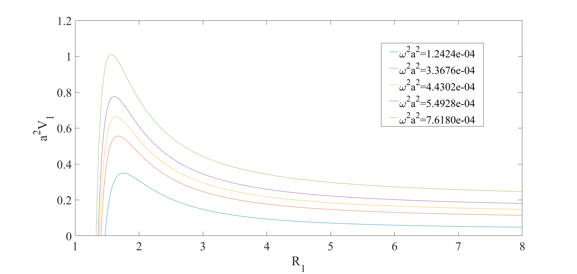
Figure 1: ${a^{2}}{V_{1}}$ for ${R_{1}}$

References

• (1) T. Regge, J. A. Wheeler, Phys. Rev. 108, 1063(1957).
• (2) C. A. Manogue, Annals of Phys. 181(1988)261.
• (3) W. Greiner, B. Mller, J. Rafelski, Quantum Electrodynamics of Strong Fields, Springer-Verlag, Berlin, 1985.
• (4) V. Cardoso, O. J. C. Dias, J. P. S. Lemos, S. Yoshida, Phys. Rev. D 70(2004) 044039.
• (5) R. Penrose, Revista Del Nuovo Cimento, 1, 252 (1969).
• (6) Ya. B. Zel‘dovich, Pis‘ma Zh. Eksp. Teor. Fiz. 14, 270 (1971) [JETP Lett. 14, 180 (1971)].
• (7) W. H. Press and S. A. Teukolsky, Astrophys. J. 185, 649 (1973).
• (8) A. V. Vilenkin, Phys. Lett. B 78, 301 (1978).
• (9) We use natural units in which $G=c=\hbar=1$.
• (10) S. Hod, Phys. Lett. B 708, 320 (2012) [arXiv:1205.1872].
• (11) Hod S. Stability of the extremal Reissner–Nordström black hole to charged scalar perturbations[J]. Physics Letters B, 2012, 713(4-5): 505-508.
• (12) S. Chandrasekhar, The Mathematical Theory of Black Holes, (Oxford University Press, New York, 1983).
• (13) R. P. Kerr, Phys. Rev. Lett. 11, 237 (1963).
• (14) The integer parameters $m$ and $l\geq\left|m\right|$ are the (azimuthal and spheroidal) harmonic indices of the scalar field modes.
• (15) S. A. Teukolsky, Astrophys. J. 185, 635 (1973).
• (16) T. Hartman, W. Song, and A. Strominger, JHEP 1003:118 (2010).
• (17) E. Berti, V. Cardoso and M. Casals, Phys. Rev. D 73, 024013 (2006) Erratum: [Phys. Rev. D 73, 109902 (2006)].
• (18) P. P. Fiziev, Class. Quant. Grav. 27, 135001 (2010).
• (19) M. Abramowitz and I. A. Stegun, Handbook of Mathematical Functions (Dover Publications, New York, 1970). 7
• (20) S. Hod, Phys. Rev. D 87, 064017 (2013) [arXiv:1304.4683].
• (21) J. M. Bardeen, W. H. Press, and S. A. Teukolsky, Astrophys. J. 178, 347 (1972).
• (22) Shahar Hod. Physics Letters B, 2016, 758(C):181-185.
• (23) It is worth noting that the lower bound on the angular eigenvalues can be saturated in the eikonal $l=m\gg 1$limit, in which case one finds the simple relation .
• (24) T. Damour, N. Deruelle and R. Ruffini, Lett. Nuovo Cimento 15, 257 (1976).
• (25) T. M. Zouros and D. M. Eardley, Annals of physics 118, 139 (1979).
• (26) S. Detweiler, Phys. Rev. D 22, 2323 (1980).
• (27) H. Furuhashi and Y. Nambu, Prog. Theor. Phys. 112, 983 (2004).
• (28) V. Cardoso and J. P. S. Lemos, Phys. Lett. B 621, 219 (2005).
• (29) S. R. Dolan, Phys. Rev. D 76, 084001 (2007).
• (30) S. Hod and O. Hod, Phys. Rev. D 81, Rapid communication 061502 (2010) [arXiv:0910.0734].
• (31) S. Hod and O. Hod, e-print arXiv:0912.2761.
• (32) S. Hod, Phys. Lett. B 739, 196 (2014) [arXiv:1411.2609].
• (33) S. Hod, Phys. Lett. B 749, 167 (2015) [arXiv:1510.05649].
• (34) S. Hod, Phys. Lett. B 751, 177 (2015).
• (35) S. Hod, Phys. Rev. D 86, 104026 (2012) [arXiv:1211.3202].
• (36) S. Hod, The Euro. Phys. Journal C 73, 2378 (2013) [arXiv:1311.5298].
• (37) S. Hod, Phys. Rev. D 90, 024051 (2014) [arXiv:1406.1179].
• (38) S. Hod, Class. and Quant. Grav. 32, 134002 (2015).
• (39) C. A. R. Herdeiro and E. Radu, Phys. Rev. Lett. 112, 221101 (2014).
• (40) Note that the coordinate $r\in[0,\infty]$is mapped into $y\in[-\infty,\infty]$ by the radial transformation.
• (41) For former analytical bounds on the instability regime of the composed Kerr-black-hole-massive-scalar-field system, see H.R. Beyer, Commun. Math. Phys. 221, 659 (2001).
• (42) S. Hod, Phys. Lett. B 746, 365 (2015) [arXiv:1506.04148].