European Football Player Valuation: Integrating Financial Models and Network Theory

Abstract

This paper presents a new framework for player valuation in European football by fusing principles from financial mathematics and network theory. The valuation model leverages a "passing matrix" to encapsulate player interactions on the field, utilizing centrality measures to quantify individual influence. Unlike traditional approaches, this model is both metric-driven and cohort-free, providing a dynamic and individualized framework for ascertaining a player's fair market value. The methodology is empirically validated through a case study in European football, employing real-world match and financial data. The paper advances the disciplines of sports analytics and financial mathematics by offering a cross-disciplinary mechanism for player valuation, and also links together two well-known econometric methods in marginal revenue product and expected present valuation.

Keywords: European Football Analytics, Soccer Analytics, Player Valuation, Financial Mathematics, Network Theory, Stochastic Processes, Passing Matrix, Markov Chains, Centrality Measures, Black-Scholes Model, Sports Economics

1 Introduction

Player valuation in European football is a complex endeavor, requiring nuanced metrics that go beyond traditional sports statistics. Due to the dearth of goals in a game, other in-game events should be utilized to understand the contribution of individual players to the team's performance. Existing methods often fail to capture the dynamic, stochastic nature of player performance and its impact on fair market valuation. This paper introduces a multi-disciplinary approach that integrates financial models with stochastic player performance models, borrowing from social network theory.

The main objectives of this research are:

1. formulate a player valuation model that integrates the passing matrix with financial mathematics, specifically stochastic asset pricing models, and

2. validate this integrated model empirically through a case study involving real-world data.

1.1 Connections with previous work

There have been, in our opinion, at least three foundational works that have provided in-depth analyses of various pieces of this puzzle. The first major work to address the link between performance and pay for athletes can be found in the paper of Scully [8]. In this paper, the author investigated the connection between a baseball team's revenue and the salary paid to the team's players. By utilizing well-known tools in labor economics, such as the marginal revenue product related to units of labor, the author derived a framework to link on-field play with salary. The second work we reference, that of Tunaru, Clark, and Viney (TCV) [10], addresses the value $V$ of a player to a team, in continuous-time, via stochastic modeling and a subsequent Black-Scholes partial differential equation (PDE.) The solution $V$ of that pde also includes the assumption that contract can be sold at the end of the term. (There have been some numerical implementations of this model, such as in [2] to value the goalkeeper of Serie A League club)) Finally, the work of Rockerbie and Easton [7] in their recent book offers a discrete, multi-period approach to contract pricing via expected present valuation and cohort analysis via a market beta. We note that Rockerbie and Easton also consider the real-option value of a player resigning between seasons, which we do not address in this paper.

1.1.1 Extension of TCV approach

In applying the principle of linking pay to a player's marginal revenue product, we seek to connect the discrete landscape of Rockerbie and Easton with the continuous stochastic modeling of Tunaru, Clark, and Viney by defining a player performance share as a stochastic process correlated to a team's revenue.

The continuous-time model in [10] proposes that a player's performance is measured by a point (or performance) score that lives on the interval $(0,\infty)$. The authors model this score for player $j$ as a geometric Brownian motion (GBM) $p_{j}$ that is also correlated to another GBM in $R$ that models the team's revenue. Next, the authors make a simplifying assumption that the sum over players $\sum_{j}p_{j}$ itself follows a GBM. The result is that the revenue earned, per point, by the team is $R/\sum_{j}p_{j}$ and the number of points $N$ that multiplies this fraction returns the performance-linked value of the player $j$ to the club, $Z_{j}:=p_{j}R/\sum_{j}p_{j}$ . We propose linking this stochastic model to that of Rockerbie and Easton by rewriting the performance linked value $Z_{j}$:

$$Z_{j}=p_{j}\cdot\frac{R}{\sum_{j}p_{j}}=\frac{p_{j}}{\sum_{j}p_{j}}\cdot R:=\pi_{j}R.$$ (1)

Here, the dynamic $\pi_{j}=\frac{p_{j}}{\sum_{j}p_{j}}$ models the normalized performance share that a player provides with their on-field play. For example, in association football if one simplifies to think of eleven key players, a uniform distribution of performance load would suggest that each player would provide $\pi_{t}=1/11=0.0909$ per game. This obviously does not happen, as there are injuries, substitutions, matchups that enhance or detract from a specific player's ability to contribute, and even worries about upcoming contract negotiations, to name a few (of a multitude of factors). Finally, there are many in-game decisions that can lead to performance estimation, and this requires the special attention of analytics providers that may keep such metrics away from public view.

To address these and other issues, our model can be calibrated using publicly available data. In doing so, we compute (augmented) passing matrices derived directly from in-game stats to apply network analysis methodologies similar to [6] and [4].

2 Risk-Neutral Model for Player Valuation

As mentioned above, we see there being two main approaches to valuing performance, using the marginal revenue product to calculate salaries and a financial derivative approach that expands functionality to allow for events such as trades, early release, and contract transfer. Our current work is also carried out in recognition of the partial link between direct and derived contract value being the stochastic modeling seen in (1).

2.1 Discrete-time models

Consider a scenario where a player can sign a contract with a team for multiple years. There is a baseline expectation for performance, but management allows for the possibility that the player can under- or over-perform, in terms of expected statistical contribution. Our model for the (stochastic) value of player $j$ in season $k$ is

$$Y_{j,k}:=\pi_{j,k}a_{k}R_{k},$$ (2)

where $a_{k}$ is the proportion of team revenue that goes to players in year $k$. That can be verified since $\sum_{j}Y_{j,k}=a_{k}R_{k}$. Note that $Y_{j,k}=a_{k}Z_{j,k}$, which connects to the work of e.g. [8], where salary can be considered as a proportion of a player's marginal revenue product, in this case represented by $Z_{j,k}$.

Assume a player can neither be released nor traded/transferred. Under the framework of risk-neutral valuation, yearly salaries for player $j$ can be computed for an $N-$year contract via the balance equation that is the swap of salary values $S$ for stochastic, performance-linked dollar revenue streams $Y$:

$$\sum_{k=1}^{N}\frac{S_{j,k}}{(1+r)^{k}}=\sum_{k=1}^{N}\frac{\tilde{\mathbb{E}}[Y_{j,k}]}{(1+r+\lambda_{j})^{k}}$$ (3)

where

• $r$ is the risk-free rate,

• $\lambda_{j}$ is the risk-premium per-season for player $j$,

• $Y_{j,k}$ represents the valuation of the player's contribution to the team for season $k$, derived from the athlete's on-field play (as in Equation (2)),

• and $S_{j,k}$ is the performance-linked salary to be computed for player $j$ for season $k$.

In this setting, salaries can be constant throughout the term, be front-loaded, or have other term-structures that match the expected present value linked to revenue streams on the right side of equation (3). This balance equation represents a way for general managers to determine a player's contract structure before the season begins. For that reason, we assume $a_{k}$ is known ahead of time to both parties.

2.2 Dynamics of Player Value Processes

Consider the univariate approach of a single player. For notational brevity, the subscript $j$ is dropped. Thus, we the need to determine the evolution of $Y$, which in equation (2) appears as the product of the two stochastic variables $\pi$ and $R$. We present the model here

$$Y_{t} =\pi_{t}a_{t}R_{t}$$ (4)

$$d\pi_{t} =\sqrt{\sigma_{\pi}\pi_{t}(1-\pi_{t})}dW^{\pi}_{t}$$

$$dR_{t} =rR_{t}dt+\sigma_{R}R_{t}dW^{R}_{t}$$

$$\rho dt =\langle dW^{\pi}_{t},dW^{R}_{t}\rangle.$$

Here, $W^{\pi}$ and $W^{R}$ are Brownian motions under the risk neutral measure $\tilde{\mathbb{P}}$, with correlation $\rho$. Note that $R$ follows a geometric Brownian motion [9]. The process defined by $\pi_{t}$ in (4) is a special (univariate) case of the Wright-Fisher process, Dirichlet process, and Jacobi process [1].

2.3 Network Theory and Passing Matrices

It is common to model financial evolutions like revenue through a geometric Brownian motion. Player performance metrics, on the other hand, have no agreed upon gold-standard. The method that we use is relatively simple, catering to the specifics of team sports that focus on frequent changes of possession. In particular, modelling of $\pi_{t}$ is done using metrics derived from passing matrices. Our primary approach borrows from and makes rigorous the work of [4]. An alternative is the pagerank matrix centrality measure as used in [6]. Appendix A.2 elucidates the pagerank approach. Both approaches row-normalize the passing matrix, so it becomes a transition matrix of a Markov chain that corresponds to the evolution of player ball possession for a given team's possession.

Specifically, we augment the passing matrix with two rows and columns, one for shots ($S$) and another for unsuccessful passes ($U$). This augmented passing matrix is denoted $P$. The shots state can either be successful shots, total shots, or a weighted combination of successful shots and missed shots. For simplicity, we simply call this state the ``shots" state. Thus, $P$ is a $(M+2)\times(M+2)$ matrix with two absorbing states ($S$ and $U$), where, for $1\leq i,j,\leq M$, $p_{i,j}$ is the probability that, if player $i$ has the ball, they pass to player $j$, and $p_{i,S}$ is the probability of transitioning to the $S$ state, and $p_{i,U}$ is the probability of an unsuccessful pass. Let $(X_{n})_{n=0}^{\infty}$ denote the team possession process, which denotes which player has the ball at step $n$ for a given team possession, governed by the Markov chain transition probabilities $P$ [5], where a ``step" means a transition in possession (pass or shot). In addition, we treat the initial distribution $\mathbb{P}(X_{0}=i)$ as the probability of player $i$ beginning a team possession (through start of half, steal, penalty, etc.). From this Markov chain, the metric of interest is

$$\mathbb{P}(A_{i}|X_{\infty}=S),\qquad A_{i}=\{X_{\ell}=i\text{ for some }\ell=0,1,\ldots\}$$ (5)

This is interpreted as the probability that, in the case of a possession ending in a shot, player $i$ was involved (in some way). This can be derived from $P$ in closed form; see Appendix A.1. The derivation illustrates impact of the initial distribution (through the law of total probability), which favors players that contribute to shots on goal by beginning possession but may not be praised through in-game stats like goals or assists. Extreme cases provide some quick insight: if $\mathbb{P}(A_{i}|X_{\infty}=S)=1$, it means all shots were filtered through player $i$ in some manner. Similarly, $\mathbb{P}(A_{i}|X_{\infty}=S)=0$ means that player $i$ was not involved in any possession that ended in a shot. Even for strong defensive players, we would still expect $\mathbb{P}(A_{i}|X_{\infty}=S)$ to be relatively large, as many shot-based possessions will involve them beginning with the ball.

In order to relate to the $\pi_{t}$ process, we

1. Assume the passing matrix varies per game, i.e. is denoted $P_{t}$. Thus we consider $\mathbb{P}_{t}(A_{j}|X_{\infty}=S)$. This is reasonable as player performance varies per game.

2. Define for each $t$ and player $j$

   $$\pi_{j,t}=\frac{\mathbb{P}_{t}(A_{j}|X_{\infty}=S)}{\sum_{i}\mathbb{P}_{t}(A_{i}|X_{\infty}=S)},$$ (6)

where the denominator sums over all players $i$ involved in the passing matrix for game $t$. This is required to ensure that $0\leq\pi_{j,t}\leq 1$, and transforms $\mathbb{P}_{t}(A_{j}|X_{\infty}=S)$ into a measure of relative player importance. An elementary computation shows $\pi_{j,t}=\mathbb{P}_{t}(A_{j}\cap\{X_{\infty}=S\})/\sum_{i}\mathbb{P}_{t}(A_{i}\cap\{X_{\infty}=S\})$ which offers an alternative interpretation.

3 Valuation Case Study for European Football

The theoretical methodologies are applied to a case study on the EPL (European Premier League). This case study showcases various uses of the $Y$ process in Equation (2). The data we use involves five seasons spanning 2018–2023. This period allowed to consider multiple players on the same team with varying contract amounts, which is difficult over a longer period due to contract expiration, trading, and retirement. Each season involves 38 games.

3.1 Setup

We first consider a discrete-time setup with years $k=0,1,\ldots$ since revenue data was only available annually. Thus $k=1$ corresponds to the 2018–2019 season, $k=2$ to the 2019–2020 season, and so forth. Then $R_{k}$ is the annual revenue, e.g. $R_{1}$ corresponds to earnings over 2018–2019. Similarly, $\pi_{j,k},k=1,2,\ldots$ are defined annually for player $j$. The information known at time $k$ is kept track through the filtration $(\mathcal{F}_{k})_{k=0}^{\infty}$. For player $j$, their fixed annual salary for season $k$ is denoted $C_{j,k}$, and the proportion of revenue allocated to players is $a_{k}$. We assume that $C_{j,k},a_{k}\in\mathcal{F}_{k-1}$, which is reasonable, as the players should know their salary and revenue share at the beginning of the season, and $\pi_{j,k},R_{k}\in\mathcal{F}_{k}$ for all $j,k$. The main quantity of interest is $S_{j,k}$, which is a rolling estimate of the expected salary that we recalculate every year (i.e. Equation (3) with $N=1$), simply termed expected salary.

3.1.1 Salary Valuation

For player $j$ we have the expected salary (at the beginning of the $k^{th}$ season) to be the expected present value of the performance-linked value $Y_{j,k}$, adjusted for survival throughout the season. We can adopt a continuous accounting for growth due to interest and survival due to injury hazard rate $\lambda$, which results in expected salary calculated in equation (7) below:

$$e^{-r}S_{j,k} =e^{-r-\lambda_{j}}\tilde{\mathbb{E}}[Y_{j,k}|\mathcal{F}_{k-1}]=e^{-r-\lambda_{j}}\tilde{\mathbb{E}}[a_{k}\pi_{k}R_{k}|\mathcal{F}_{k-1}]$$ (7)

$$=e^{-r-\lambda_{j}}a_{k}R_{k-1}\tilde{\mathbb{E}}[\pi_{k}e^{r-\sigma_{R}^{2}/2+\sigma_{R}\Delta W^{R}_{k}}|\mathcal{F}_{k-1}],$$

where $\Delta W^{R}_{k}=W^{R}_{k}-W^{R}_{k-1}$. To simplify the calculation (and provide a closed likelihood for estimation), we use a discrete approximation $\pi_{k}=\pi_{k-1}+\sigma_{\pi}\sqrt{\pi_{k-1}(1-\pi_{k-1})}\Delta W^{\pi}_{k}$. Using $dW_{t}^{\pi}dW_{t}^{R}=\rho dt$, yields $(\Delta W_{t+1}^{R},\Delta W_{t+1}^{\pi})$ to be bivariate normal with correlation $\rho$, and hence

$$S_{j,k} =e^{r-\lambda_{j}}a_{k}R_{k-1}\left[\pi_{k-1}+\tilde{\mathbb{E}}[\sigma_{\pi}\sqrt{\pi_{k-1}(1-\pi_{k-1})}\Delta W^{\pi}_{k}e^{-\sigma_{R}^{2}/2+\sigma_{R}\Delta W^{R}_{k}}]\right]$$ (8)

$$=e^{r-\lambda_{j}}a_{k}\pi_{k-1}R_{k-1}\left[1+\rho\sigma_{\pi}\sigma_{R}\sqrt{(1-\pi_{k-1})/\pi_{k-1}}\right].$$

Alternatively, one can note that an application of Itô's formula for $d(\pi_{t}R_{t})$ shows

$$\tilde{\mathbb{E}}[\pi_{t+dt}R_{t+dt}|\mathcal{F}_{t}]=\pi_{t}R_{t}\left(1+r+\rho\sigma_{\pi}\sigma_{R}\sqrt{(1-\pi_{t})/\pi_{t}}\right)dt.$$

Valuation then can utilize a fully discrete approximation (with $dt=1$). By adopting a discrete accounting for yearly interest rate $r$ and risk premium $\lambda$, one obtains the expected salary computed in equation (7) below:

$$\frac{S_{j,k}}{1+r} =\frac{1}{1+r+\lambda_{j}}\tilde{\mathbb{E}}[Y_{j,k}|\mathcal{F}_{k-1}]=a_{k}\tilde{\mathbb{E}}[\pi_{k}R_{k}|\mathcal{F}_{k-1}]$$ (9)

$$\Rightarrow S_{j,k} =\frac{1+r}{1+r+\lambda_{j}}a_{k}\pi_{k-1}R_{k-1}\left[1+r+\rho\sigma_{\pi}\sigma_{R}\sqrt{(1-\pi_{k-1})/\pi_{k-1}}\right],$$

In the analysis below, we utilize the continuous (8), but one can note its similarity with (9). In particular, both are dependent on the previous year player performance $Z_{j,k-1}=\pi_{j,k-1}R_{k-1}$, current year player share $a_{k}$, with an accumulation factor depending on $r$ and discounted by risk premium $\lambda_{j}$. Additionally, both contain a factor that adjusts these values proportional to a covariance term involving $\rho\sigma_{\pi}\sigma_{R}$ (akin to a market $\beta$).

3.1.2 Toward Options on Player Value

A question that naturally arises in a manager's mind is how a player performs during the season compared to their guaranteed contract value. Thus, is useful to consider $C_{j,t}-Y_{j,t}$ which represents, for player $j$, the difference between their quoted salary for game $t$ and their observed player value for that game. For example, an insurance could be derived for a player's mid-season under-performance, or used to price trade related contracts. Since our setting does not provide $R_{t}$ for non-integer times, we make this rigorous by considering

$$\mathcal{F}^{\texttt{game}}_{t}=\sigma(\pi^{\texttt{game}}_{s},R_{\lfloor s\rfloor},a_{\lfloor s\rfloor+1},s\leq t)$$ (10)

where $\lfloor x\rfloor$ is the largest integer less than or equal to $x$, and two processes:

$$\Delta_{j,k} =C_{j,k}-S_{j,k}\in\mathcal{F}_{k-1},\qquad k=1,2,\ldots,$$ (11)

$$\Delta^{\texttt{game}}_{j,t} =C_{j,t}-S^{\texttt{game}}_{j,t}\in\mathcal{F}^{\texttt{game}}_{t-1/52},\qquad t=\frac{1}{52},\frac{2}{52},\ldots,$$ (12)

where $t$ spans the dates that games are played (assumed weekly), and $C_{j,k+1/52}=\cdots=C_{j,k+1}$ is the constant weekly game check for year $k$, and $S^{\texttt{game}}_{j,t}$ is based off of the process $Y^{\texttt{game}}_{j,t}=\pi^{\texttt{game}}_{j,t}a_{t}R_{t}$ (see (13)). Similar to $C$, we assume $a_{k+1/52}=\cdots=a_{k+1}$. Since $\pi^{\texttt{game}}$ is defined weekly but $R$ is not, we assume $\rho=0$ for any calculation for game related processes. For notational simplicity, denote $k=\lfloor t\rfloor+1$ and $t$ is a non-integer. A similar calculation as in Section 3.1 yields

$$e^{-rt}S^{\texttt{game}}_{j,t}=e^{-rt}\tilde{\mathbb{E}}[Y^{\texttt{game}}_{j,t}|\mathcal{F}_{t-1/52}]\quad\Rightarrow\quad S^{\texttt{game}}_{j,t}=e^{r(t-k+1)}\pi^{\texttt{game}}_{j,t-1/52}a_{k}R_{k-1},$$ (13)

i.e. last year's game performance multiplied by player share, and last years revenue accumulated by the risk free rate $e^{r(t-k+1)}$ for the $t-k+1=t-\lfloor t\rfloor$ weeks elapsed since the beginning of the season. Since game appearance is reflected in the $\pi^{\texttt{game}}$ process, we assume $\lambda_{j}=0$ for $S^{\texttt{game}}$.

In terms of application, if $\Delta^{\texttt{game}}_{j,t}$ in Equation (11) widens beyond a certain threshold, the manager may be tempted to release or trade the player during the upcoming season, if possible. Or, if there was an insurance product that would compensate a team for a player's under-performance, payments could be triggered when $\Delta_{k}$ exceeds a threshold value. With granular revenue data, these could be valued using the $R_{t}$ process. For example, an option on player underperformance could be linked to a payoff of the form $(K-Y_{j,t})_{+}$, where $(x)_{+}$ denotes the positive part of $x$. This is large when $Y_{j,t}$ is small (relative to $K$), which benefits the purchaser in the case of underperformance.

3.2 Estimation and Calibration

Assume a risk free rate of $r=0.02$. Revenue and salary data is available annually, and game data is available for every game over the seasons of interest. The unknown parameters are the player specific $\pi_{j,0},\sigma_{\pi,j}$, $\rho_{j}$, $\lambda_{j}$ (over $j$), and $\sigma_{R}$. As mentioned, we consider $K=5$ seasons. For robustness, $\sigma_{R}$ is first estimated through maximum likelihood estimation (MLE) using $R_{0},\ldots,R_{K}$, knowing that $\log(R_{k}/R_{k-1})\overset{\text{iid}}{\sim}N(r-\sigma^{2}_{R}/2,\sigma^{2}_{R}),$ with $R_{0}$ available from historic data. Then, for the player specific parameters, the discrete approximation for $\pi$ shows for all $k$ that $[\pi_{j,k},\log(R_{k})]^{\top}|\mathcal{F}_{k-1}\sim N\left(\mu_{j,k-1},\Sigma_{j,k-1}\right),$ where

$$\mu_{j,k-1} =\begin{bmatrix}\pi_{j,k-1}\\ r+\log(R_{k-1})-\frac{1}{2}\sigma_{R}^{2}\end{bmatrix},$$ (14)

$$\Sigma_{j,k-1} =\begin{bmatrix}\sigma_{\pi,j}^{2}\pi_{j,k-1}(1-\pi_{j,k-1})&\rho_{j}\sigma_{\pi,j}\sigma_{R}\sqrt{\pi_{j,k-1}(1-\pi_{j,k-1})}\\ \rho_{j}\sigma_{\pi,j}\sigma_{R}\sqrt{\pi_{j,k-1}(1-\pi_{j,k-1})}&\sigma_{R}^{2}\end{bmatrix}$$ (15)

Consequently, the parameters $\pi_{j,0},\sigma_{\pi,j},\rho_{j}$ are estimated using maximum likelihood estimation. See Appendix C for all estimates obtained in the upcoming analysis and a related discussion.

To estimate the risk premium $\lambda_{j}$, first denote $m_{j,k}$ as the number of games player $j$ missed due to injury or violations (e.g. red card suspensions), so that $n_{j,k}=N_{j,k}-m_{j,k}$ as the number of games played over season $k$. Note that $N_{j,k}=38$ is the maximal amount (if a player is available for all games). This is the case for most players. In a few circumstances, like due to when a player is traded onto a team in the middle of a season, we may have $N_{j,k}<38$. Injury rates are estimated over the entire period as $\lambda_{j}=\sum_{k}m_{j,k}/\sum_{k}N_{j,k}$, following an approach similar to [10, 2].

In terms of the player shares, practically speaking $a_{k}$ should be known from the club in question. However, this data is unavailable so it is estimated through

$$a_{k}=\left[\sum_{i}\frac{N_{i,k}}{38}C_{i,k}\right]/R_{k},$$ (16)

which is exactly the fraction of the money that goes out to players for season $k$. Note that the factor $N_{i,k}/38$ compensates for the case of players being traded or bought mid-season.

Finally, in order to calibrate $\pi$, recall that $\pi_{j,k}$ depends on a passing matrix originally defined per game. In order to obtain an annual estimate, we consider a multi-step process. First, consider $Q_{t}^{\texttt{game}}$, which is the augmented sample passing frequency matrix, i.e. where the $i,j$ entry is the number of passes that went from player $i$ to $j$ in game $t$, augmented with columns so that $[Q_{t}^{\texttt{game}}]_{i,U}$ is the number of unsuccessful passes from player $i$ and $[Q_{t}^{\texttt{game}}]_{i,S}=w_{S}\cdot n_{i,\text{score}}+(1-w_{S})\cdot n_{i,\text{miss}}$, where $n_{i,\text{score}}$ is the number of times player $i$ scored (implicitly for game $t$), and $n_{i,\text{miss}}$ is the the number of missed shots. Initial calibrations showed that $w_{S}=10/11$ works well, which counts a missed shot as worth 1/10 of a score. The initial distributions (only required in intermediate calculations) are similarly estimated per-game using frequencies of when a player began possession of a play (beginning of half, steal, etc.). Then $P_{t}^{\texttt{game}}$ is the stochastic (row-normalied) version of $Q_{t}^{\texttt{game}}$, so that the $i,j$ entry is the empirical probability of the next transference of ball ownership ends in state $j$ if it begins with player $i$. For each player $j$, and game $t$, $\pi_{j,t}^{\texttt{game}}$ is derived from $P_{t}^{\texttt{game}}$ using the methods described in Section 2.3 and Appendix A.1.

Granular game data allows obtaining (for each player $j$) the game processes $\pi_{j,t}^{\texttt{game}}$ which are observed at the per-game (weekly) level, defined for the annual times at which games were played. For example, $t=1/52$ if a game was played on the first week of the season, and $t=38/52$ for the final game. Similarly, $t=1+1/52$ would be the first game of the second season. Since we require an annual estimate for valuation purposes, we estimate for $k=1,2,\ldots$,

$$\pi_{j,k}=\frac{1}{n_{j,k}}\sum_{k-1<t<k}\pi_{j,t}^{\texttt{game}},$$ (17)

i.e. their average over the season, for the games that they were present. Remark: The individual $\pi_{j,t}^{\texttt{game}}$ are also used in Section 3.3.1 below.

3.3 Model Application and Results

The primary focus of our analysis utilizes Liverpool and three key players: Virgil van Dijk, Mohamed Salah, and Trent Alexander-Arnold. This choice is rooted in the fact that their contracts were active, with varying values, during the 2018–2023 period. Appendix B extends a similar analysis to Arsenal and Brighton for a broader perspective. Additionally, Appendix C gives all estimated parameters.

Figure 1: Salary related and $\pi$ processes for Liverpool. Two dashed lines are $C_{k}$ (paid salary), and $S_{k}$, weekly (in £). The historic $\pi_{t}^{\texttt{game}}$, overlayed with its average $\pi_{j,k}$ from Equation (17) (thick solid line)

These players, as prominent members of the squad, provide a practical basis for sanity-checking the estimates. Specifically, their $\pi$ values should reasonably align with $0.0909\approx 1/11$, given that a starting squad comprises 11 players.

Looking individually at the players, Virgil van Dijk's compensation appears well-aligned with his contributions through the 2018–2021 period, as indicated by the close correspondence between $C_{k}$ and $S_{k}$. Although model suggests that the pay raise for the 2021–2023 season is potentially unwarranted, it is worth noting that Virgil missed most of the 2020–2021 season due to injury, deflating all salary estimates by his $\hat{\lambda}_{j}$.

Looking at Mohamed Salah, his $\pi$ exhibits significant variability, likely influenced by his role as a key scorer (e.g. guaranteed to be in all successful shots, if he was the only scorer for a game, or on the opposite end if another player was the only scorer). His average $\pi$ is typically higher than that of his peers, correlating with higher salary estimates. Spanning 2018–2022, we observes undervaluation (accentuated from 2019–2021), so it is unsurprising to see a pay raise for 2022–2023 (to approximately £350,000). Although Salah is clearly crucial to the teams performance and the data suggested undervaluation, the model suggests the magnitude of the raise to be unwarranted.

Looking at Trent Alexander-Arnold, Liverpool's salary increase (18–19 to 19–20, and 20–21 to 21-22) align with our measure of increased salary estimates. Indeed, his paid salary is approximately equal to the estimate for 2021–2022. Otherwise he is generally underpaid.

3.3.1 Assessing Player Salary Misalignment

This section provides an empirical application of the techniques discussed in Section 3.1.2. In particular, the same players for Liverpool are considered, and the processes $\Delta_{j,k}$ and $\Delta^{\texttt{game}}_{j,t}$ are displayed in Figure 2 (see Appendix B for Arsenal and Brighton).

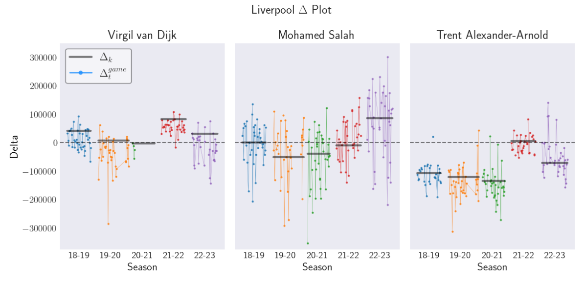
Figure 2: Time series of $\Delta_{k}$ (annual) and $\Delta_{t}^{\text{game}}$ (per game) for Liverpool.

First, note the interpretation of $\Delta$: $\Delta>0$ means the player is underperforming (relative to the contract) and $\Delta<0$ indicates overperformance. Since $\Delta_{k}$ is simply the difference of $C_{k}$ and $S_{k}$ from Figure 2, we verify many of the observations (comparing the thick grey line in Figure 2 with the difference of $C_{k}$ and $S_{k}$ in Figure 1. However, the game-to-game analysis through $\Delta_{t}^{\texttt{game}}$ provides a more granular explanation. This is especially clear with Virgil van Dijk, where the purely annual view suggested slight overpayment, but Seasons 20–21 and 22–23 specifically highlight games where Virgil generally outperforms his contract. Salah shows higher variation than the other players, as was also apparent by $\pi_{t}^{\texttt{game}}$ in Figure 1.

4 Discussion and Conclusion

This work fills a vital niche between the stochastic modeling of [10] and the marginal revenue product perspective of [7] through development of a financial model that integrates network theory and stochastic modelling. While this discussion is applied to teams in the European Premier League, it easily extends to other leagues, and can be utilized in other sports where player impact can be encapsulated primarily through a data matrix, such as an augmented passing matrix (e.g. hockey). This versatile framework offers a practical and reliable tool for financial decision-making in sports teams, contributing a novel and empirically aligned financial framework to sports analytics.

The core of our research lies in bridging the gap between traditional valuation methods and a sophisticated financial model that utilizes stochastic processes to represent player performance shares. Our model's alignment with empirical data from the European Premier League serves as a testament to its validity. It passes critical sanity checks and closely mirrors real-world scenarios, providing a reliable tool for financial valuation in sports. Section 3.3 empirically justifies calibration of the player performance process $\pi$ and how it relates to player valuation, which is a key contribution of this paper. Further, Section 3.3.1 showcases a weekly dynamic view of $\Delta^{\texttt{game}}_{j,t}$, the difference between salary and player value, providing insight into how more complex financial contracts could be priced using this framework.

Our methodology is subject to the limitations of data availability and granularity. However, as discussed in previous sections, this provides an opportunity for future enhancements, particularly with more detailed financial data.

Although our analysis did not focus specifically on lower string players, it is worth mentioning that the model and its calibration is designed to compensate this, as their lower playtimes will result in a lower $\pi$, consequently contributing to $Y$. On the other hand, alternative calibration methods should be considered for goalie valuation, as they generally have deflated probabilities of involvement in scoring of a goal (usually only in the case that a possession began with them). This is a topic for future work.

4.1 Future Directions

Our current work has focused on player compensation that is directly linked to both performance and revenue. The correlation coefficient $\rho$ in (4) represents the primary connection between a team's revenue and a salaried player's performance. However, there are many players on a team and the sum of their contributions via team play also factor into to a team's revenue stream. To capture this secondary effect of performance correlation among teammates, one direction is to extending the TCV [10] model via multiple, correlated stochastic processes for player performance shares $\big{\{}\pi^{(j)}_{t}\big{\}}_{j=1}^{M}$. This would lead to a system of SDE's. Additionally, one could directly incorporate a ``"team market beta" to value a team as more than the sum of its parts.

The interpretation of a player's value to their team as a transferable asset is modeled via the framework of financial derivatives of $Y$ in [10]. We propose that insurance against poor play can also be contingent on $Y$ in a similar fashion, such as a rebate if the gap $C-Y$ exceeds a threshold $K$. This involves proposing a pricing mechanism for such an object using $Y$ directly in the formula for $\Delta$'s in a credit default swap framework.

Utilizing granular (i.e. per game) data and such contracts would provide useful insights into the effects of parameters on pricing. Akin to market volatility affecting the price of financial options, we would expect quantities like $\sigma_{\pi}$ to have a larger effect on these contracts. Insights into $\partial/\partial\sigma_{\pi}$ would illustrate how player variability influences contract price. This idea can be applied to any of the aforementioned contracts.

Appendix A On Passing Matrix Markov Chains

A.1 Derivation of Markov Chain Probability

The goal is to obtain $\mathbb{P}(A_{i}|X_{\infty}=S),$ where $A_{i}=\{X_{\ell}=i\text{ for some }\ell=0,1,\ldots\}$, in terms of the transition matrix $P$ and initial distribution. Note that $P$ is a finite Markov chain. For simplicity, assume that all states communicate except for the two absorbing states ($S$ and $U$). It is well known that one can find the probability of absorption into one of these states starting in state $j$. This event is denoted by e.g. $\{X_{\infty}=S\}$. Now,

$$\mathbb{P}(A_{i}|X_{\infty}=S) =\frac{\mathbb{P}(A_{i}\cap\{X_{\infty}=S\})}{\mathbb{P}(X_{\infty}=S)}.$$

for the numerator

$$\mathbb{P}(A_{i}\cap\{X_{\infty}=S\}) =\sum_{j}\mathbb{P}(A_{i}\cap\{X_{\infty}=S\}|X_{0}=j)\mathbb{P}(X_{0}=j)$$

$$=\sum_{j}\left[\mathbb{P}(X_{\infty}=S|X_{0}=j)-\mathbb{P}(\{X_{\infty}=S\}\backslash A_{i}|X_{0}=j)\right]\mathbb{P}(X_{0}=j)$$

where $\{X_{\infty}=S\}\backslash A_{i}$ is the set difference, i.e. the case of absorption into $S$ but player $i$ never having possession. This can be computed by considering a new Markov chain that treats state $i$ as absorbing, and finding the probability of reaching $S$ before $i$ (see [5] for details). For the denominator,

$$\mathbb{P}(X_{\infty}=S)=\sum_{j}\mathbb{P}(X_{\infty}=S|X_{0}=j)\mathbb{P}(X_{0}=j)$$

A.2 Pagerank

Pagerank is a well known matrix centrality measure that has been applied in European football, see e.g. [6]. One way to derive pagerank that is in line with our methods is as follows. If $P$ is the original probability transition matrix, then pagerank is the stationary (i.e. long-run) distribution obtained from a modified probability transition matrix

$$\lambda P+\frac{1-\lambda}{|P|}E$$ (18)

where $E$ is a $|P|\times|P|$ matrix with entries of $1$'s, and $\lambda$ is a multiplicative factor, commonly $\lambda=0.85$. So, the transition probabilities change from $p_{ij}$ to $\lambda p_{ij}+\frac{1-\lambda}{|P|}$. The interpretation is that instead of the ball possession being determined purely through $p_{ij}$, instead, being at any given state $i$, the possession can change to all other players (equally probable) with probability $1-\lambda$; otherwise the original passing probability is used with probability $\lambda$.

Preliminary analysis utilized pagerank but ultimately found that it severely undervalued key scorers. This makes sense if one considers the derivation in Equation (18), which has no bearing on the worth of a score. Similarly, defensive efficiency is not taken into account (whereas it is in the initial distribution in the previous section), and neither is missed passes. This preliminary analysis also considered an augmented matrix that contained a highly weighted column for scoring, but it only offered marginal improvement. It is possible that a further modification could yield usable results, but that is left to future work.

Appendix B Analysis of Additional Teams

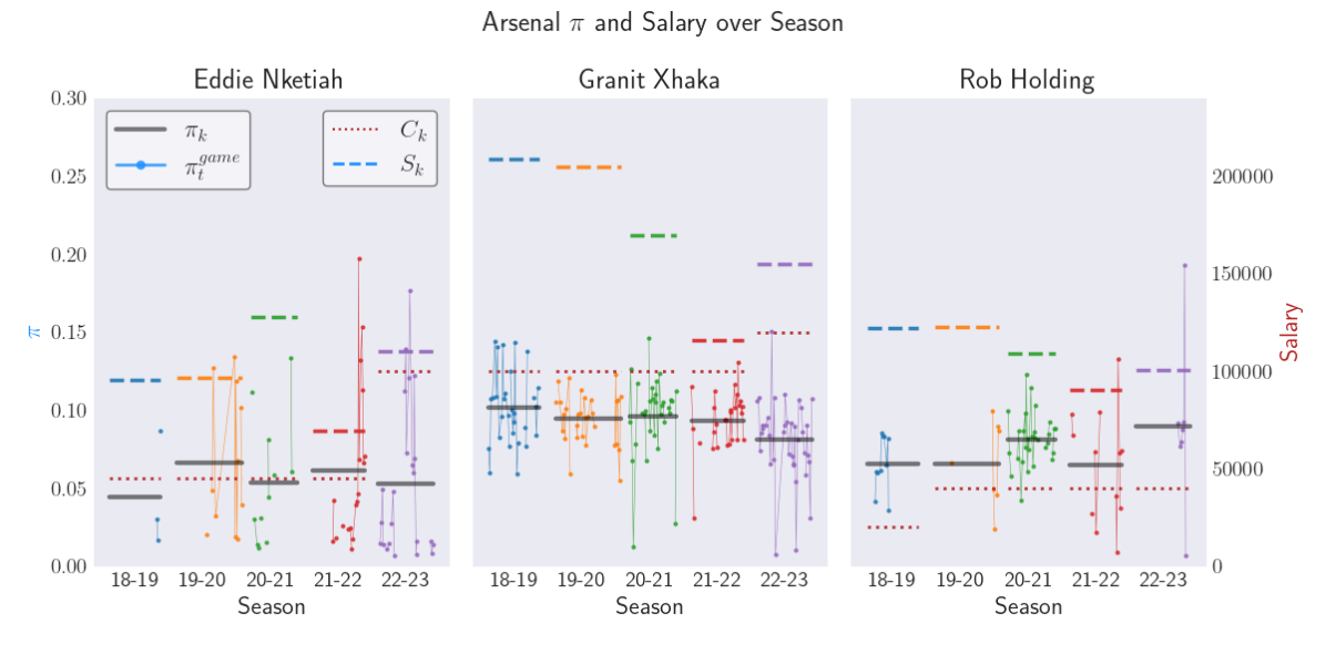
Figure 3: Salary related and $\pi$ processes for Arsenal. Two dashed lines are $C_{k}$ (paid salary), and $S_{k}$, weekly (in £). The historic $\pi_{t}^{\texttt{game}}$, overlayed with its average $\pi_{j,k}$ from Equation (17) (thick solid line)

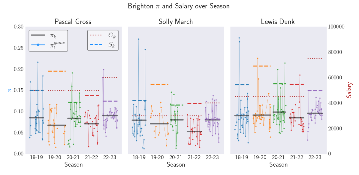
Figure 4: Salary related and $\pi$ processes for Brighton. Two dashed lines are $C_{k}$ (paid salary), and $S_{k}$, weekly (in £). The historic $\pi_{t}^{\texttt{game}}$, overlayed with its average $\pi_{j,k}$ from Equation (17) (thick solid line)

Arsenal:

Looking at Figure 3, Eddie Nketiah is missing for many games. This is partly because he entered the 2018–2019 season mid-season as a trade. In 2019–2020 and 2020–2021, his involvement is sparse, likely due to being a lower string player. Our estimated salary is higher for those early years, which matches his raised salary in 2022–2023. This is somewhat predicted by stellar performance toward the end of the 2021–2022 season. In some sense, the model anticipates the salary raise, similar to both Salah and Alexander-Arnold of Liverpool. Granit Xhaka and Rob Holding are two interesting cases. Rob has many games missing. However, even as a lower string player, the $\pi$ values are telling the story of being impactful, between around 0.07 to 0.10. That player share is quite significant, wondering if additional attention should be brought to Rob. The profile of Granit Xhaka's $\pi$'s are similar to van Dijk and Alexander-Arnold and generally tells a similar story to Alexander-Arnold in terms of slight underpayment. However, according to the $\pi$'s, his performance declined significantly in 2022–2023.

Brighton:

Looking at Figure 4, the story is similar to Liverpool. Pascal Gross shows valuation to be as expected. The pay raise for 2022–2023 is minimal, which could reflect desire for a contract extension but not to the point of a high expense. Solly March tells a similar story to Pascal. Lewis Dunk has a similar profile to Mohamed Salah. In particular, he has highly fluctuating $\pi$'s, and an observed underpayment until a salary increase in 2022–2023 (which, similar to Salah, may have been more than it was worth, as the $\Delta$ for that year is nearly £20,000.)

Appendix C Parameter Estimates

All estimation and calibration is done according to Section C. Estimates are reported in Tables 1 (player specific) and 2 (team specific). It is worth noting that the $a_{k}$ values differ from the wage/revenue ratio in [3] due to various factors (including those wages including staff and differences in reporting).

		$\rho$ estimated			$\rho=0$
Team Name	Player Name	$\hat{\pi}_{0}$	$\hat{\sigma}_{\pi}$	$\hat{\rho}$	$\hat{\pi}_{0}$	$\hat{\sigma}_{\pi}$	$\hat{\lambda}$
Liverpool	Mohamed Salah	0.109	0.026	-0.506	0.103	0.025	0.011
Liverpool	Virgil van Dijk	0.089	0.014	-0.286	0.087	0.014	0.207
Liverpool	Trent Alexander-Arnold	0.084	0.020	-0.070	0.084	0.020	0.043
Arsenal	Granit Xhaka	0.102	0.022	0.206	0.102	0.022	0.136
Arsenal	Eddie Nketiah	0.043	0.056	-0.400	0.043	0.056	0.051
Arsenal	Rob Holding	0.064	0.060	-0.370	0.064	0.059	0.203
Brighton	Pascal Gross	0.083	0.056	0.393	0.083	0.056	0.075
Brighton	Solly March	0.077	0.074	-0.097	0.077	0.074	0.169
Brighton	Lewis Dunk	0.089	0.029	-0.231	0.089	0.029	0.055

Table 1: Parameter estimates for each player under analysis, for the cases of $\rho$ estimated and $\rho=0$.

Team Name	$\hat{\sigma}_{R}$	$a_{1}$	$a_{2}$	$a_{3}$	$a_{4}$	$a_{5}$
Liverpool	0.112	0.219	0.233	0.255	0.208	0.239
Arsenal	0.092	0.307	0.298	0.307	0.216	0.264
Brighton	0.159	0.237	0.292	0.285	0.214	0.182

Table 2: Estimates of $\hat{\sigma}_{R}$ and calibrated values for each team's player share ($a_{k}$) process.

Somewhat surprisingly, seven out of the nine $\hat{\rho}$ values are negative. We attribute this to a variety of factors, generally stemming from lack of data. From a statistical standpoint, estimating three parameters with only ten data points is a difficult task. From a sports analytic standpoint, it seems hard to detect how a player's aggregate performance in a given season is going to affect the revenue for that season. The motivation for including $\rho$ in the first place is due to a hypothesized effect on game-day revenue, for example due to fan favorite players and hot streaks. In aggregation, that is much harder to detect. There may also be a misalignment in the sense that performance of last week would affect gameday revenue in the current week. It is worth noting that despite these estimates being counter intuitive, their effect is relatively small; recall Equation (7) which displays it as a multiplicative effect of $(1+g)$, with $g$ depending on $\rho$. A quick calculation using the estimates from Table 1 for Mohamed Salah reveals this factor to be (using $\hat{\pi}_{0}$ for $\pi_{k-1}$) $(1-0.004213)=0.9958$. The table also reveals that the $\hat{\pi}_{0}$ and $\hat{\sigma}_{\pi}$ estimation is mostly unaffected when moving from the $\rho$ estimated to $\rho=0$ case.

Looking at $\hat{\sigma}_{\pi}$, these values are generally low, which is unsurprising as they are estimated through an average of seasonal data and the annual values do not fluctuate much. These would be much higher if we considered the game process (note that this would have a larger effect on the ``$1+g$'' factor mentioned in the last paragraph).

References

- Bakosi et al. [2013] J. Bakosi, J. Ristorcelli, et al. A stochastic diffusion process for the Dirichlet distribution. International Journal of Stochastic Analysis, 2013:1–7, 2013.
- Coluccia et al. [2018] D. Coluccia, S. Fontana, and S. Solimene. An application of the option-pricing model to the valuation of a football player in the'serie a league'. International Journal of Sport Management and Marketing, 18(1-2):155–168, 2018.
- Deloitte Sports Business Group [2019–2023] Deloitte Sports Business Group. Annual review of football finance 2019–2023. https://www2.deloitte.com/content/dam/Deloitte/uk/Documents/sports-business-group/deloitte-uk-annual-review-of-football-finance-2023.pdf, 2019–2023.
- Duch et al. [2010] J. Duch, J. S. Waitzman, and L. A. N. Amaral. Quantifying the performance of individual players in a team activity. PloS one, 5(6):e10937, 2010.
- Grimmett and Stirzaker [2020] G. Grimmett and D. Stirzaker. Probability and random processes. Oxford university press, 2020.
- Pena and Touchette [2012] J. L. Pena and H. Touchette. A network theory analysis of football strategies. arXiv preprint arXiv:1206.6904, 2012.
- Rockerbie and Easton [2020] D. W. Rockerbie and S. T. Easton. Contract Options for Buyers and Sellers of Talent in Professional Sports. Springer Nature, Switzerland, 2020. doi: https://doi.org/10.1007/978-3-030-49513-8.
- Scully [1974] G. W. Scully. Pay and performance in major league baseball. The American Economic Review, 64(6):915–930, 1974.
- Shreve et al. [2004] S. E. Shreve et al. Stochastic calculus for finance II: Continuous-time models, volume 11. Springer, 2004.
- Tunaru et al. [2005] R. Tunaru, E. Clark, and H. Viney. An option pricing framework for valuation of football players. Review of financial economics, 14(3-4):281–295, 2005. doi: https://doi.org/10.1016/j.rfe.2004.11.002.