Microwave signal processing using an analog quantum reservoir computer

Abstract

Quantum reservoir computing (QRC) has been proposed as a paradigm for performing machine learning with quantum processors where the training is efficient in the number of required runs of the quantum processor and takes place entirely in the classical domain, avoiding the issue of barren plateaus in parameterized-circuit quantum neural networks. It is very natural to consider using a quantum processor based on microwave-frequency superconducting circuits to classify microwave signals that are analog—continuous in time. However, while theoretical proposals of analog QRC exist, to date QRC has been implemented using circuit-model quantum systems—artificially imposing a discretization of the incoming signal in time, with each discrete time point input by executing a gate operation. In this paper we show how a quantum superconducting circuit comprising a linear oscillator coupled to a single qubit can be used as an analog quantum reservoir for a variety of classification tasks, achieving high accuracy on all of them. Our quantum system was operated without artificially discretizing the input data, directly taking in microwave signals (centered at ${\sim}$6 GHz). Our work does not attempt to address the question of whether or when QRCs could provide a quantum computational advantage in classifying pre-recorded classical signals. However, beyond illustrating that sophisticated tasks can be performed with a very modest-size quantum system and inexpensive training, our work opens up the possibility of achieving a different kind of quantum advantage than a purely computational advantage: superconducting circuits can act as extremely sensitive detectors of microwave photons; our work demonstrates processing of ultra-low-power microwave signals in our superconducting circuit, and by combining sensitive detection with QRC processing within the same system, one could achieve a quantum sensing-computational advantage, i.e., an advantage in the overall detection and analysis of microwave signals comprising just a few photons.

Introduction

Over the last decade, researchers in quantum information processing have broadly divided their efforts into two distinct but complementary themes. In one, the focus has been on realizing the building blocks for large-scale, fault-tolerant quantum processors [28, 24, 7], which would enable running algorithms such as Shor’s or Grover’s at meaningful scale. In another, there has been a push to realize quantum systems comprising tens to hundreds of qubits or qumodes, but without error correction, and to explore what can be done with such noisy, pre-fault-tolerance systems—often denoted as noisy, intermediate-scale, quantum (NISQ) devices [38]. Quantum computational supremacy with such NISQ devices has been demonstrated [2, 49], but there has been much less progress on achieving quantum advantage in practically relevant applications than had been hoped for as NISQ machines began to be created [35]. There have been many NISQ studies on quantum machine learning [5], and in this area too, quantum advantage for problems of broad practical interest has remained elusive [40, 8]. A major open question is whether one can achieve any practically relevant advantage for machine learning with NISQ systems.

One of the main approaches to performing quantum machine learning with NISQ machines is to use parameterized quantum circuits as quantum neural networks [42, 25, 9], which are a subclass of variational quantum algorithms, in which parameters of a quantum circuit are adjusted, usually by a classical co-processor, so that the quantum circuit incrementally approaches carrying out a desired computation. This approach, however, typically suffers from barren plateaus [32, 44, 31, 1], which mean that, in practice, it is difficult or impossible to perform the optimization required to set circuit parameters [19]. Inspired by the framework of reservoir computing [29, 39, 26, 17] in classical machine learning, quantum reservoir computing (QRC) [15, 14, 18] has emerged as an approach to quantum machine learning that entirely avoids barren plateaus by performing all the learning in the classical domain. They key idea of a QRC is that a quantum system (called a quantum reservoir) can generate nonlinear, high-dimensional features of inputs to it, and that these features can be used to perform machine-learning tasks purely by training a classical linear transformation. QRC can be implemented both in the circuit model of quantum computation [14] and with analog quantum dynamical systems [30, 6]. However, experimental demonstrations to date have been performed with digital quantum circuits [37, 10, 27, 34, 48, 41, 21] that have limited the complexity of tasks that can be performed, in part due to an input bottleneck imposed by the use of discrete gates to input temporal data using a series of separate, imperfect gates.

The aim of our work is to demonstrate a proof-of-principle for a new application of and approach to quantum machine learning with NISQ devices that overcomes or sidesteps the challenges in training and inputs noted above. We use the driven, continuous-time analog quantum nonlinear dynamics of a superconducting microwave circuit as a quantum reservoir to generate features for classifying weak, analog microwave signals (Fig. 1a). We use repeated measurements of the reservoir both to extract features that contain information about temporal correlations in the input data, as well as to induce non-unitary dynamics. Our use of a continuous-variable system in our quantum reservoir grants us access to a substantially larger Hilbert space than would be the case with a qubit-only system with equally many hardware components. In relying on continuous-time dynamics, our approach is similar to other proposals for analog NISQ processors and simulators [36, 16, 11], which aim to avoid the overhead that imposing a discrete-time (circuit-model, gate-based) abstraction causes. Analog operation grants us an even more important ability however, which fundamentally distinguishes our work from prior experimental demonstrations of quantum machine learning on circuit-model quantum processors: it allows our device to directly, natively receive weak analog microwave signals, and to immediately leverage analog quantum information processing to extract relevant features of the signals for classification.

This small shift in context has important implications, offering a new path to practical quantum advantage with NISQ hardware. Rather than focusing on using NISQ hardware to perform computation on pre-recorded, digital data, we instead use quantum hardware to perform computation on real-time analog signals that interface directly with our microwave superconducting device. Our experiments do not address the question of whether a QRC can achieve a quantum computational advantage, since our experimental device is small enough to be easily classically simulable. However, our demonstrations suggest a route to achieving a quantum advantage of a different kind: an advantage in the quantum detection and processing of weak microwave signals, allowing quantum hardware to extract complex information of interest from dim, analog signals in ways that would be noisier with a conventional classical approach. This type of quantum advantage, arising from a combination of quantum sensing with extraction of complex features about the sensed signal, is discussed in general terms as a route to quantum advantage with quantum machine learning in Ref. [8]. Our work shows that when classical signals comprising just a few photons have entered an analog quantum reservoir, they can be classified using our QRC approach. If one combines this analog quantum processing with a sensitive quantum detector of microwave radiation, as has already been previously demonstrated using superconducting circuits [46, 45, 4, 3], then one can construct a system that achieves a quantum advantage in the task of combined sensing and signal processing.

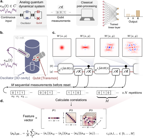
Figure 1: Analog signal classification with a continuous-variable quantum reservoir computer (QRC) using measurement trajectories. (a.) We perform machine learning using a quantum system consisting of an oscillator coupled to a qubit. Analog signals are fed into our analog quantum dynamical system, continually displacing the oscillator mode while the qubit is protectively measured. The measurement trajectories provide complex features a digital linear layer can use to perform classification on a variety of tasks. (b.) The signals interface directly with the qubit-oscillator system, composed of a 3D aluminum cavity hosting a transmon qubit. (c.) Simulated Wigner distributions of the oscillator state through various stages of the reservoir dynamics. The dynamics include entanglement-generating unitary evolution, and projective measurements of both the qubit and cavity. The back-action produced by the measurements add to the non-classical features generated by the entangling unitaries. The balance of measurements and unitaries, which do not commute with each other in our implementation, lead to complex correlations in the measurement trajectories. (b.) The digital linear layer performs classification based on a feature vector, which we construct using the expectation values of the central moments $\mu_{p}$, which capture the essential correlations in the reservoir dynamics.

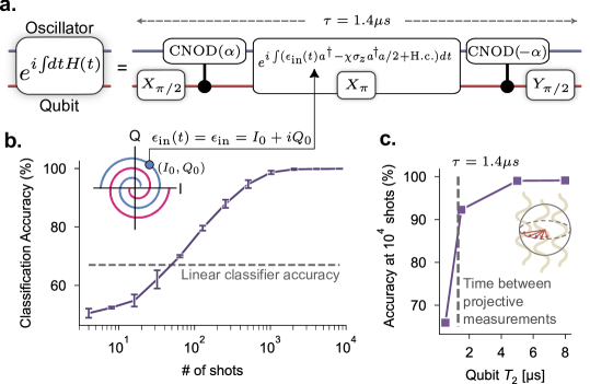
Figure 2: Reservoir protocol overview with an example time-independent classification task (a) The unitary dynamics in our reservoir is generated by control pulses that serve to entangle the qubit with the oscillator before the analog input is received by the oscillator. For tasks where the analog data is time-independent, the dynamics is fully gate-based, and the oscillator is dis-entangled with the qubit before the qubit and oscillator measurements. For details of the motivation behind the particular unitaries implemented for our reservoir, see Appendix C. (b) (Inset) An illustrative machine learning example is the classification of time-independent signals from two arms of a Spiral distribution defined in the signal $I-Q$ plane. Unlike classical machine learning, in quantum machine learning, the performance is unavoidably impacted by sampling noise. Here, we plot the classification accuracy of the spiral task with increasing number of shots. Also plotted is the performance of a linear layer acting directly on the two-dimensional $I,Q$ data, indicating that non-linearity is required to perform this task with sufficient accuracy. (c) Classification accuracy at $10^{4}$ shots as a function of qubit coherence time that we tune via resonator-induced dephasing during the classification (see Appendix D). While we see a large drop in classification performance when the qubit coherence time is heavily suppressed and the system is completely disentangled, the performance only begins to suffer once the qubit $T_{2}$ approaches the duration between measurements.

Experimental setup and protocols

Our quantum reservoir, composed of a long-lived cavity mode coupled to a transmon qubit (Fig. 1b), can be modeled with the rotating-frame Hamiltonian,

$$H=-\chi a^{\dagger}a\frac{\sigma_{z}}{2}+\epsilon^{*}(t)a+\epsilon(t)a^{\dagger}+\Omega_{x}(t)\sigma_{x}+\Omega_{y}(t)\sigma_{y},$$ (1)

where $\sigma_{z}$ is the Pauli operator on the qubit subspace of the transmon, $a$ is the photon annihilation operator of the cavity mode, and $\chi$ is the nonlinear interaction strength (see Appendix C for details). The right-most term of Eq. 1 describes the unitary control of the qubit, and the second term describes both the encoding of the input data $\epsilon_{\mathrm{in}}(t)$, and unitary control of the oscillator mode, i.e., $\epsilon(t)=\epsilon_{\mathrm{in}}(t)+\epsilon_{\mathrm{control}}(t)$. Equation 1 describes the unitary dynamics, which is complemented by non-unitary dynamics generated by the back-action from qubit measurements interspersed throughout the evolution.

The oscillator and qubit control drives used in our work realize a reservoir that consists of a series of entangling unitaries interleaved with qubit and oscillator measurements (Fig. 1c). The analog input results in a time varying displacement of the cavity, which streams in concurrently with control drives implementing an entangling unitary. Following the unitary, we perform a qubit measurement, and then the parity of the oscillator state is measured [43, 20] (see Appendix D). The parity measurement projects the oscillator state into either even or odd super-positions of Fock states, giving us sensitive information about photon number changes of oscillator while inducing non-classical features to the state via measurement back-action. In effect, our construction implements a sequence of non-commuting measurements (see Appendix C), generating correlated measurement distributions that can then be used as complex output features.

The measurement outcomes are used to construct output feature vectors to be fed into the linear layer (Fig. 1a), but this can be done in a few different ways. In principle, with repeated applications of the unitary, we generate a sample of bitstrings with $2^{M}$ possible outcomes, where $M$ is the number of measurements. The outcomes can be counted to directly form a sample probability distribution over measurement trajectories, which can then be used as a high-dimensional output feature vector after obtaining a sufficient number of samples $N$. While this approach has the benefit of capturing all information in the measurement distribution [21], it can generally suffer from poor scaling in sampling noise, requiring $N\sim 2^{M}$ shots in the worst case [47]. On the other hand, one could average over the measurements directly [48, 41]; however, this has the unwanted effect of averaging over and removing quantum correlations. Here, we construct an output feature vector from estimates of successive central moments $\mu_{1},\mu_{2},\mu_{3},\ldots$ of the underlying distribution over measurement trajectories (Fig. 1d). Additionally, given finite memory in our reservoir, we choose to only use correlations between measurements at most 3 measurements apart. This approach, inspired by Ref. [26], has the benefit of leveraging the hierarchy of noise in the central moments, while capturing the essential correlations in the dynamics to achieve high accuracy even in the few-sample regime. For a detailed analysis of the construction of our reservoir output features with comparisons, see Appendix E.

Results

Classification of time-independent signals

To illustrate the scheme proposed in this work, we begin with an example classification using our quantum reservoir by performing binary classification task of time-independent signals. Figure 2a describes the control drives in more detail. For time-independent input data, the two-dimensional input data is encoded as the $I$ and $Q$ quadratures of an analog signal resonant with the oscillator frequency, which displaces the cavity. Here, time-independence describes the signal refers to the fact that it is on resonance the oscillator mode, and thus has no time-dependence in the oscillator’s rotating frame (such that $\epsilon_{\mathrm{in}}(t)=\epsilon_{\mathrm{in}}$ in Eq. 1). For time-independent tasks, the signal bandwidth is set by its duration, and therefore the resultant displacement is essentially conditioned on the qubit in the ground state due to the cross-Kerr interaction.

The unitary encoding the input displacement is complimented by control drives that entangle the qubit and cavity via a series of conditional displacements [13] and qubit rotations. For time-indepedent tasks, this set of unitaries effectively impart a geometric area enclosed by the cavity trajectory onto the qubit, such that the information of the phase of the unknown input signal can be extracted via a qubit measurement (see Appendix C for details of this unitary). In Appendix H, we show the ability of the set of unitaries implemented here (Fig. 2a) to be able to approximate any scalar function of the input signal when the signal is time-independent. For all results presented, we implement our reservoir unitary with these control drives across all tasks, with 4 applications of the unitary interleaved with qubit and oscillator-parity measurements.

The binary classification task we perform here is: Two distributions of time-independent signals, completely characterized by the signal’s in-phase ($I$) and quadrature ($Q$) components, are distributed along two separate “arms of a spiral” in the $I-Q$ plane (Fig. 2b). The classification task is: given a displacement described by the points $I$ and $Q$ sampled from either signal distribution, figure out which distribution the signal came from. This simple task has the feature that, if one feeds in the inputs directly into a linear layer, this would classify with an accuracy of no more than $67\%$ – just above random guessing of $50\%$ (Fig. 2b). As a point of comparison with non-linear digital networks, we found that a 64-dimensional, two-layer digital reservoir was needed to achieve the same performance as our quantum reservoir for this task (see Appendix J for details of this comparison).

To probe the role of quantum in our reservoir, we performed the same classification task, but with reduced coherence time in the qubit during the reservoir execution. This is achieved by populating the lossy readout resonator with photons that send the qubit to the center of the Bloch-sphere when the readout resonator is traced out (see Appendix D). With $T_{2}\rightarrow 0$, we effectively removed all entanglement with the cavity, and observed two things: a dramatic reduction in classification performance, and importantly, $T_{2}$ only began affecting the performance once it was on the order of the reservoir duration, after which the qubit was projected. This latter point highlights an important benefit of repeated measurements in our reservoir construction, i.e. while entanglement is important for generating complex distributions in our setup, we are able to classify and capture information much longer than the qubit decoherence time, requiring only that the oscillator state is coherent at long times.

Classification of radio-frequency (RF) communication modulation schemes

We showcase our reservoir in a real-world setting by discriminating time-dependent radio-frequency (RF) signals from 10 different digital modulation schemes. Digital modulation schemes encode binary information in discrete ‘symbols’ encoding in sequential time-bins. For example, Binary Phase-Shift Keying (BPSK) encodes binary data in discrete phase jumps of a signal, such that a symbol $0$ ($1$) maps to a phase flip of $0$ ($\pi$). While BPSK only contains one bit of information per symbol, other encoding schemes such as 32 Quadrature Amplitude Modulation (32QAM) can encode 5 bits per symbol. These and other encodings can be represented in a constellation diagram (Fig. 3a), which denotes the potential $(I,Q)$ values a signal can take for each symbol. A given string of digital data can then be encoding in a time-domain signal by sequentially choosing points in the constellation diagram with a given symbol rate, denoting the rate at which the symbol will change. For typical WiFi signals this is around 250 kHz per subchannel [23].

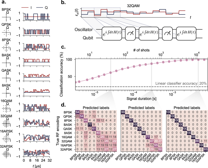
Figure 3: Classification of radio-frequency (RF) communication modulation protocols. (a) Description of the dataset for digital modulation schemes used in this experiment. In conventional digital modulation schemes, one encodes data in the amplitude and phase of the signal. The modulation schemes can be represented by a “constellation diagram” in $(I,Q)$ space (left), where point represents one of the possible choice of $(I,Q)$ values to enclode a symbol, with example time traces (right). (b) These signals are broken up and fed into our reservoir. (c) The performance of the reservoir as a function of the shots taken in real time (see text). The top row contains the corresponding duration of the radio frequency signal required. As the number of shots increases, the fluctuations in the measurement distribution reduces, resulting in a higher classification accuracy. For context, a classical linear classifier applied directly on the input data achieves only $20\%$ accuracy, independent of the duration of the signal. The error bars of the accuracy curve have been omitted here due to the fact they are too small. (d) Confusion matrix for the QRC at 32, 512, and $10^{4}$ shots, showing that the reservoir confuses only a few classes at the highest shots.

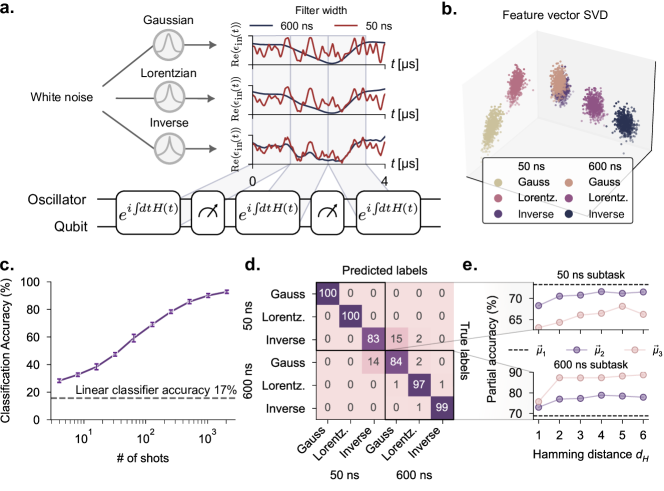
Figure 4: Classification of filtered noise (a) We classify various fast and slow noisy signals by applying a moving average on stochastic white-noise signals. Three different filters are used for the moving averages: a Gaussian filter, a Lorentzian, and an inverse power law. For each filter, we generate stochastic analog signals based on both a 50 ns filter width, and a 600 ns filter width, with the latter being on the order of the measurement rate. Example time traces are given for the real part of an example stochastic white noise signal passed through each of the filters. We divide up these stochastic signals and send to the QRC to then distinguish the noise source. (b) Visualization of the high-dimensional output feature space using Singular-Value-Decomposition. Each point corresponds to a different signal over 2000 shots taken in real time (see text). (c) Classification accuracy as a function of the number of shots using third order moments as the output feature. Our reservoir reaches 93% accuracy in about 2000 shots, corresponding to about 10 ms of the signal received. (d) Confusion matrix of the task taken at 2000 shots. (e) Participation of the mean and the off-diagonal elements of the second- and third-order moments in the classification accuracy within the subtasks of classifying different noise sources with fixed filter width. We see that for signals with long coherence times, higher order measurement correlations are important, while for fast signals, the mean dominates in the performance contribution.

For this task, we generated RF signals by encoding random digital strings into the 10 different modulation schemes with a fixed symbol rate of around 2 symbols per $\mu$s. The duration of these signals can last much longer than the reset rate of our system. Importantly, we did not repeat the same signal to artificially reduce the sampling noise associated with each input data, as this would not typically be applicable in a real-world setting. Instead, the measurement statistics were generated by sampling the signal in real time. Consequently, what we refer to as ‘shots’ in a real-time task do not correspond to identical repetitions of the experiment, but instead, is the number of resets we performed while acquiring the signal, which changed from shot to shot. In effect, each different encoding scheme produces a unique “fingerprint” of distribution over measurement outcomes, and it is the goal of the linear layer is to separate these distributions with as high accuracy as possible.

Figure 3c shows the accuracy in classifying digitally modulated RF signals with increasing number of shots, compared with the performance of a linear classifier. We note that in less than a millisecond, or with less than 2000 symbols, the reservoir was able to classify which of the 10 classes a given signal belongs to with $>$ 90% accuracy when using 8 qubit-cavity measurements. A linear classifier can only achieve 20% classification accuracy for this task, even with infinite symbols. The confusion matrix between the difference classes at 32, 512, and $10^{4}$ shots is displayed in Fig 3d, which is nearly diagonal.

Classification of filtered noise

Next, to demonstrate the performance of our QRC on continuous-time data, and with a task that requires both long-term and short-term memory in the quantum reservoir, we performed the following classification task: input data assumed to have come from a source of white noise is filtered using a moving-average filter having one of three filter shapes (Gaussian, Lorentzian and inverse-power-law), and one of two window widths ($50$ ns and $600$ ns), and the task is to identify both the filter shape and window width (Fig. 4a), leading to six possible output classes. The filter functions were normalized so that the photon number distributions generated by the time-dependent displacements are identical up to the filter width. This normalization was applied to ensure that the task is not trivially solvable by just measuring the mean photon number (see Appendix F).

Because all the signals used in this dataset are noise with zero mean, a linear classifier would do no better than random guessing. On the other hand, Figure 4b visually shows (using singular-value-decomposition on the output feature space) that the quantum reservoir was able to peel apart the different noise distributions. In this space, we see that the different classes are nearly all linearly-separable, with some overlap between the long-tailed but fast 50-ns inverse-power-law noise class, and the slow 600-ns Gaussian noise class. On the task of classifying over six different sources of noise, we achieved 93% accuracy (Fig. 4c) in only 2000 shots. As seen in the confusion matrix in Fig. 4d, the primary confusion at 2000 shots was distinguishing between the 50-ns inverse-power-law noise class and the 600-ns Gaussian noise class, as expected from the overlap in the SVD of the feature space.

Finally, we compared the ability of our reservoir to understand long vs short correlations in input signals. For this, we deconstructed the full 6-class task into two sets of 3-class classification tasks, where each set has the same correlation length and are only distinguishable by the filter window type (see Fig. 4d and e). The class of signals with coherence length of 50 ns highlight the convenience of our input encoding scheme, i.e. feeding signals directly into the cavity mode without the need to sample the signal discretely in time. In contrast, classification of the class of signals with coherence lengths of $600$ ns require correlations of the reservoir dynamics beyond that of the measurement rate. To highlight the advantage of our scheme, we simulate the performance of a reservoir with that of a recent gate-based protocol where the input is sampled discretely in time [48]. Our simulations results, in Appendix  G, highlight the advantage of our protocol when the sampling rate of the input is slow, which can arise in experiment such as finite pulse durations and latency introduced by the FPGA classical comparison.

Figure 4e looks at the participation of the different moments $\mu_{k}$ of the measurements in the classification accuracy of the 50 ns subtask (top), and the 600 ns subtask (bottom). Here, the output features are constructed by the mean $\mu_{1}$, or the off-diagonal elements of the moments $\mu_{2}$ and $\mu_{3}$ as a function of the hamming distance, allowing us to probe the contribution of the moments as a function of the locality of the correlations. For the 50 ns subtask, we see that the most important contribution is the mean, with the second order moment being the next-most important contribution, and the third-order moment being relatively unimportant. In stark contrast, the third-order moment is most important for the 600-ns subtask, suprisingly yielding nearly 90% using non-local third-order correlations alone. The ability to distinguish stochastic signals among the combined six classes demonstrate the ability of our reservoir to capture both slow and fast features of microwave signals.

To understand the role of the Hilbert space dimension on the performance of the reservoir, in Appendix  G, we simulate an extension of our quantum reservoir with multiple qubits. Our results point to an increase in classification accuracy with every additional inclusion of a qubit to the reservoir, for the same duration of input signal received.

Discussion

In summary, we have experimentally realized an analog quantum reservoir computer (QRC) and demonstrated its ability to directly process microwave analog input signals without discretization, achieving high classification accuracy on three different tasks. Previous demonstrations of quantum reservoir computing have used multi-qubit, gate-based quantum reservoirs [48, 37, 10, 41, 27, 34, 21]. In contrast, we perform machine learning directly on analog signals fed into a single oscillator coupled to a transmon qubit. Intuitively, an analog (continuous-time, partially continuous-variable) quantum reservoir should be well-matched to processing microwave signals that may be continuous in time as well as amplitude. In addition to demonstrating accurate classification of microwave signals in our experiments, we also performed a direct comparison with a state-of-the-art discrete-time, gate-based QRC approach in simulation, and found that a continuous-time reservoir outperforms a discrete-time reservoir when the input signals contain temporal variations fast relative to the discretization time.

While our quantum reservoir only has two constituents (an oscillator and a qubit) we are nevertheless able to construct high-dimensional output features from the reservoir—which is essential in reservoir computing [12]—by performing multiple ($M$) projective measurements of the qubit during the dynamics between resets of the reservoir. We have proposed and demonstrated using central moments to construct output feature vectors from correlations between the measurement results. This approach has two key benefits. First, it allows one to control the dimension of the feature vector through the choice of the maximum order of correlators to include—which is important because while it is important to have high dimensionality, it is also possible for the dimensionality to be too high. This is in contrast to, for example, constructing a feature vector from the histogram of all $2^{M}$ possible bitstring outcomes of performing $M$ qubit measurements—in which case the feature vector has fixed size $2^{M}$. Second, central moments provide a natural way to extract non-trivial correlations in the measurement results, which is best explained with an example: a correlation $\braket{x_{1}x_{2}}$ may be dominated by the product $\braket{x_{1}}\braket{x_{2}}$, and we use the approach of central moments to subtract this trivial component. We performed experiments that compared the central-moment-correlators feature-vector construction with the histogram feature-vector construction and found that the former approach yielded better accuracy.

For any quantum neural network, including QRC approaches, a central concern is to what extent one can achieve high accuracy on a particular task without needing an impractical number of shots [47]. Ref. [21] recently reported that certain functions—termed eigentasks—can be constructed with low error from quantum reservoirs even when the number of shots is modest, giving evidence that for some tasks, sampling noise need not be overwhelming. In our experiments, we found that it was possible to achieve high accuracy for all the tasks we attempted while needing only $10^{3}$–$10^{4}$ shots (depending on the task). There is important future work to be done in exploring the tradeoffs between reservoir size (e.g., number of oscillators or qubits), number of measurements $M$ between reservoir resets, feature-vector dimension (dependent both on $M$ and the choice of order of correlators to include), and number of shots required for both training and inference. Because in our construction the feature-vector dimension can be adjusted without changing $M$, it is possible to, for example, explore the impact of feature-vector dimension and content on task accuracy while using the same number of measurements and a fixed number of shots.

Our quantum reservoir is small enough that it is easy to simulate classically, so it does not—at its present size of just one cavity and one qubit, at least—provide a quantum computational advantage. We nevertheless performed two studies to try understand what role quantumness is playing in our reservoir in achieving the classification accuracies that we experimentally observed. First, we showed that by artificially decreasing the coherence time of the qubit through injection of noise, the classification accuracy decreased. Second, we performed simulations of our QRC with a classicalized model of the quantum reservoir, in which no entanglement could be present, and found that this classicalized simulation of our QRC achieved worse accuracy than our quantum experimental results. These studies provide strong evidence that quantumness plays an important role in the operation of our quantum reservoir.

With improved quantum hardware, we anticipate that it will be possible to carry out even more sophisticated tasks than what we have already demonstrated. Increasing the coherence time of the oscillator would enable us to perform many more measurements (the qubit’s coherence time is, favorably, less important in our scheme because our protocol involves repeatedly projectively measuring the qubit). While we analytically showed in Appendix H the ability of our QRC to be able to approximate any scalar function of the input signal when the signal is time-independent, provided the number of measurements $M$ performed is large enough, there remains the open theoretical question of the expressiveness of the QRC when the input signal is time-dependent. Extending the qubit-oscillator system to have multiple qubits and/or multiple oscillators would provide a larger Hilbert space and the potential for more complex dynamics and entanglement, which should in turn support more sophisticated computations.

It is an open question if QRC—using the type of reservoir we considered in this paper, or any other—can, when implemented with NISQ hardware, achieve a quantum computational advantage over the best classical machine learning approaches, just as it is unclear if any quantum-machine-learning method can [8]. We did not investigate the potential for purely computational quantum advantage: our quantum reservoir is small enough to be easily classically simulable, and we did not vary its size in experiment to systematically study scaling. In the setting of processing prerecorded signals (which can be copied and replayed with negligible added noise), our single-oscillator, single-qubit QRC would offer no computational advantage over the best classical algorithms running on classical digital computers. However, our work opens up the possibility to experimentally achieve a different type of quantum advantage than a purely computational one. If one performs quantum processing on data obtained by a quantum sensor, there is the potential for an advantage that is a hybrid of being due to the advantage of quantum sensing and of quantum computing [8]. Our work suggests the feasibility of concretely realizing this kind of hybrid quantum sensing-computational advantage, where the quantum sensor is a superconducting circuit that can detect classical microwave radiation with high quantum efficiency and low noise [46, 45, 4, 3], and the processing of the received signal can happen within the same superconducting circuit as the detection occurred. Our experiments have shown that it is possible to accurately classify signals using a superconducting circuit even when there are only a few photons of signal in the superconducting circuit within any single run. Combining this with a sensitive quantum detector could lead to quantum smart sensors—quantum versions classical in-sensor processors [50]—that can reliably extract information from weak microwave signals in a way that exceeds the accuracy of any equivalent classical system.

Note added: During the final stages of our work, we became aware of a related effort, Ref. [22], and we coordinated to release our papers simultaneously. Ref. [22] introduces a protocol for quantum reservoir computing with temporal data. Similar with theirs, our approach also uses mid-circuit measurements. We experimentally realized our reservoir with an analog quantum system, in contrast to their implementation, which was with a discrete-time, gate-based quantum system.

Data and code availability

All data generated and code used in this work is available at: https://doi.org/10.5281/zenodo.10432778

Author contributions

A.S. designed and carried out the hardware experiments and performed the data analysis. S.P. performed the numerical simulations of the quantum system and helped to optimize the experimental protocol with early contribution from J.K.. V.K. performed the numerical simulations of the classicalized quantum system, and performed the comparisons with classical machine-learning methods. V.F. oversaw the design and creation of the superconducting device by S.R. and others. A.S. and V.F. set up the cryogenic and microwave apparatus. S.R. calibrated the superconducting device with A.S. and V.F.. Y.C. and X.W. performed the theoretical analysis of the expressivity in Appendix H. T.O., L.G.W. and P.L.M. conceived the project, and T.O. and J.K. performed initial numerical simulations to validate the concept. A.S., S.P. and P.L.M. wrote the manuscript with input from all authors. P.L.M. supervised the project.

[sections]

Appendix Contents

[sections]0

 

Appendix A Summary of methods

Reservoir unitary

To design a good reservoir computer capable of performing machine learning on a variety of tasks, one needs to implement control drives that can efficiently capture important information of the input and perform a non-trivial and non-linear map to output features. Here, our reservoir is composed of alternating unitaries and measurements. The design of the former is motivated to harness the quantum properties of the dynamical system to generate entanglement and the design of the latter to generate non-linear operations on the state of our reservoir via measurement back-action. Here we summarize the control drives and measurements we use and their effect on the reservoir dynamics, both in the context of time-dependent and time-independent signals.

For time-independent signals, the unitary implemented in our reservoir (see Fig. 2b) can be approximated by the following set of unitaries (see Appendix C)

$$U_{1} =X_{\pi/2}$$ (2)

$$U_{2} =D(\alpha)|g\rangle\langle e|+D(-\alpha)|e\rangle\langle g|$$ CNOD (3)

$$U_{3} =D(\beta)|g\rangle\langle g|+|e\rangle\langle e|$$ Input (4)

$$U_{4} =X_{\pi}$$ (5)

$$U_{5} =U_{3}=D(\beta)|g\rangle\langle g|+|e\rangle\langle e|$$ Input (6)

$$U_{6} =D(-\alpha)|g\rangle\langle e|+D(\alpha)|e\rangle\langle g|$$ CNOD (7)

$$U_{7} =Y_{\pi/2}.$$ (8)

This combination of unitaries enclose a loop in the oscillator’s phase space. The area of this closed loop, which depends on the phase of the unknown displacement $\beta$, imparts a geometric phase onto the qubit. In this work, we perform this unitary directly after a qubit measurement without reset. The action of the combined unitary on the qubit prepared in the ground or excited state, and for an arbitrary cavity state, is

$$U|g\rangle =U_{7}U_{6}U_{5}U_{4}U_{3}U_{2}U_{1}|g\rangle$$ (9)

$$=\frac{1}{\sqrt{2}}D(\beta)[i\sin(A-\pi/4)|g\rangle+\cos(A-\pi/4)|e\rangle]\otimes|\mathrm{cavity}\rangle$$ (10)

$$U|e\rangle =\frac{1}{\sqrt{2}}D(\beta)[i\cos(A-\pi/4)|g\rangle+\sin(A-\pi/4)|e\rangle]\otimes|\mathrm{cavity}\rangle$$ (11)

where $A=2|\alpha||\beta|\sin(\delta)=i(\alpha\beta^{*}-\alpha^{*}\beta)$ is the geometric phase enclosed by the oscillator trajectory, and dependent on the phase difference $\delta$ between a known displacement $\alpha$, and the unknown displacement $\beta$. The probability of measuring the qubit in the excited state given it started out in the ground state, $P_{e|g}$, and the probability of measuring excited given the qubit start in the excited state, $P_{e|e}$ are given by

$$P_{e|g}=\cos(A-\pi/4)^{2}\qquad\qquad P_{e|e}=\sin(A-\pi/4)^{2}$$ (12)

The equation relates the qubit probability to the phase of the input displacement, which is otherwise challenging to extract in a setup with only qubit measurements.

For general time-dependent signals, the closed loop formed by Eqs. 2-8 is broken, and the system is entangled before the measurement. While this can be hard to study analytically in the general case, we take a look at a special case of time-dependent signals, namely those of Fig. 3. Here, the signal is time-dependent up to half the duration, so that the signal is effectively two time-independent signals combined. As a result, Eqs. 4 and 6 are no longer equal, but each still a time-independent displacement, and thus, the effects of the cross-Kerr, as discussed in Appendix C, do not hinder the interpretation of the effective gate-based model. For such input signals, the state of the system just before measurement is

$$|\psi\rangle=\frac{1}{2}[e^{iA_{i}}D(\beta_{i})+e^{-iA_{j}}D(\beta_{j})]\otimes|g,\mathrm{cavity}\rangle+\frac{1}{2}[e^{iA_{i}}D(\beta_{i})-e^{-iA_{j}}D(\beta_{j})]\otimes|e,\mathrm{cavity}\rangle,$$ (13)

where $\beta_{i}$ is the displacement just before the qubit flip (corresponding to Eq. 4 for this time-dependent set of tasks), and $\beta_{j}$ is the displacement after (Eq. 6). $A_{i}=\alpha\beta_{i}$ is the phase acquired after two non-orthogonal displacements. When $\beta_{i}=\beta_{j}$ we recover the dynamics for time-independent signals.

Repeated measurements

The unitaries described above are followed by a qubit measurement, then a parity measurement. For time-independent signals, the qubit and cavity are disentangled at the end of the unitary, and the effect of the unitary on the cavity is just a displacement. Thus we can ignore any affects of the qubit measurement on the cavity. The state of the cavity after $M$ repeated measurements and $M$ time-independent displacements can be effectively described as

$$|\mathrm{cavity}\rangle=\ldots P_{p_{4}}D(\beta)P_{p_{3}}D(\beta)P_{p_{2}}D(\beta)P_{p_{1}}D(\beta)|0\rangle,$$ (14)

where $P_{x_{n}}$ is the projector of the $n$th parity measurement $\Pi$ with measurement outcomes $x_{n}=\{+,-\}$. In Appendix H, we show that by sampling the parity measurements alone combined with the linear layer, we can realize (but not limited to) the following vector space of funtions:

$$\mathcal{H}_{\mathrm{parity}}:=\left\{c_{0}+c_{1}e^{-2|\beta|^{2}}+c_{2}\left(e^{-2|\beta|^{2}}\right)^{2}+\cdots+c_{k}\left(e^{-2|\beta|^{2}}\right)^{k}:c_{0},c_{1},\dots,c_{k}\in\mathbb{R}\right\}.$$ (15)

Output feature encoding & the linear layer

In reservoir computing, the outputs of a reservoir, called feature vectors, are sent to a trained linear layer. Here, we briefly outline the motivation and construction of the feature vectors and the training algorithms used in this manuscript.

In general, sampling over all possible measurement trajectory outcomes and generating a probability distribution contains all the information one can extract from a quantum system. However, not all the information plays an equal role for finite samples. Thus, for our work here, we use a physically motivated output feature vector that efficiently captures the relevant information for a linear layer. The output feature vectors for our reservoir are generated from computed correlations of measurement outcomes. The $p$-th order correlations are characterized by the $p$-th central moment $\mu_{p}$ of the underlying distribution of measurement trajectories. The elements of $\mu_{p}$ are

$$(\mu_{p})_{ijkl\ldots}=\frac{1}{N_{\mathrm{shots}}}\sum_{n}^{\mathrm{N_{shots}}}(x_{ni}-\langle x_{i}\rangle)(x_{nj}-\langle x_{j}\rangle)(x_{nk}-\langle x_{k}\rangle)(x_{nl}-\langle x_{l}\rangle)\ldots,$$ (16)

where $x_{in}$ is the $n$th repeated measurement outcome of observable $x_{i}$ for a total of $N_{\mathrm{shots}}$ repetitions, and $\langle\ldots\rangle$ is the expectation value taken over repetitions. For the results presented in the main text, we use only up to third-order correlations. Additionally, due to the finite memory present in our reservoir, we only keep correlations between nearest, next-nearest, and next-next-nearest measurements. See Appendix E for details and motivation behind this choice.

For machine learning with reservoir computing, the only component of the reservoir that is trained is a linear layer applied to the above feature vectors. The linear layer is an $R\times C$ matrix $W_{\mathrm{train}}$ and applied to the $R$-dimensional feature vector $x$, and biased with a $C$-dimensional vector $v_{\mathrm{train}}$:

$$y=W_{\mathrm{train}}x+v_{\mathrm{train}}.$$ (17)

Here $C$ is equal to the number of classes in the data set. The largest elements of $y$ corresponds to the class that the reservoir predicts the given input data point $x$ belongs to. To train the weight matrix $W_{\mathrm{train}}$, we either use a pseudo-inverse method to minimize the mean squared error (MSE) between $W_{\mathrm{train}}x$ and $y$, or backpropagation to minimize the MSE after a softmax function. Both methods are described in more detail in Appendix E. In the main manuscript, we present results for whichever performed the best.

Appendix B Experimental setup

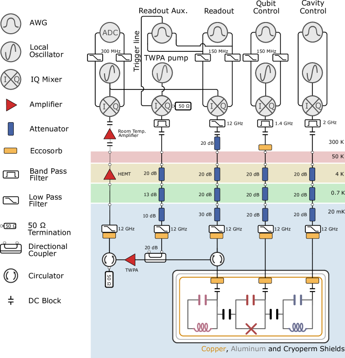
Figure M1: Wiring diagram. Experimental setup for control hardware, cable routing, and shielding for our device.

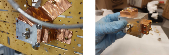
Figure M2: Photo of device The device consists of a on-chip transmon and a co-planar waveguide resonator mounted inside a high-purity Aluminum cavity. The package is mounted to a gold-plated copper breadboard at the mixing-chamber plate of a dilution refridgerator.

The device used in this paper consists of an oscillator, a 3D stub post cavity made from high-purity 4N Aluminum treated with an acid etch, and a transmon qubit. The transmon, made of Niobium, is fabricated on a resistive silicon chip, along with an on-chip readout resonator also made of Niobium. The single chip hosting the transmon and the readout resonator is mounted in the 3D cavity package using copper clamps. The cavity and the copper clamp contain copper films for thermalization directly to gold-plated copper breadboard at the mixing chamber plate of the dilution refrigerator (Fig. M2). The device is shielded with Copper coated with Berkeley Black, and two types of magnetic shields: Aluminum, and Cryoperm (Fig. M1).

The control pulses for the qubit and the storage are synthetized using Zurich Instruments (ZI) HDAWG, which have a baseband bandwidth of 1 GHz. These are upconverted using Rohde & Schwarz SGS100A, which are signal generators with built-in IQ mixers. These built-in mixers are used for all frequency conversions with the exception of the readout. The readout pulses are synthesized and digitzied using ZI UHFQA, and are up-converted and down-converted using Marki mixers (MMIQ-0416LSM-2), with a split LO from a single SGS100A. Readout signals are first amplified with a traveling-wave Josephson Amplifier (TWPA), a quantum-limited amplifier. The TWPA typically requires large pump tones, so we gate it with a trigger line from the readout AWG which combines with the CW pump tone in an IQ mixer (as a makeshift fast switch). The readout signals are then further amplified with a High-electron mobility transistor (HEMT) ampliflier at the 4K stage, and again amplified with a room temperature amplifier (ZVA-1W-103+ from Mini-Circuits) and filtered. The digitizer on the ZI UHFQA converts to the analog response to a digital signal and integrates it to produce a binary outcome depending on the qubit state.

For the experiments that intentionally suppress the qubit $T_{2}$ via resonator induced dephasing via pumping of the readout resonator, we use an additional ZI HDAWG channel that combines with the AWG of the ZI UHFQUA. This was mostly a choice out of convenience, as the AWG of the ZI UHFQUA has limitations that made characterizations tricky.

Appendix C System Hamiltonian & Reservoir description

Hamiltonian description

We approximate our transmon as a qubit. Our qubit-oscillator system is well described by the Hamiltonian [Blais_2021]:

$$H/\hbar=\omega_{q}q^{\dagger}q+\omega_{a}a^{\dagger}a-\chi q^{\dagger}qa^{\dagger}a-\chi^{\prime}q^{\dagger}qa^{\dagger 2}a^{2}-K_{q}q^{\dagger 2}q^{2}-Ka^{\dagger 2}a^{2}+\Omega(t)(q+q^{\dagger})+\epsilon(t)(a+a^{\dagger}),$$ (18)

where $a$ is the annihilation operator for the oscillator mode, and $q$ is the annihilation operator for the qubit mode, $\omega_{a}$ and $\omega_{q}$ are the frequencies of the oscillator and qubit mode respectively, $\chi$ and $\chi^{\prime}$ are the dispersive shift and the cavity state-dependent dispersive shift respectively, $K$ and $K_{q}$ are the self-Kerr of the oscillator and the transmon anharmonicity respectively. The values for these parameters, as well as values for decay rates are listed in Table S1. For the construction of our drives, we ignore the self-Kerr or the oscillator as well as the higher-order cross-Kerr. We note that these are indeed present, but for the purposes of a quantum reservoir, only add to the complexity of the dynamics. Finally, moving to the rotating frame of the qubit and cavity mode, we arrive at the Hamiltonian in Eq. 1.

Parameter	Mode(s)	Symbol	Value
Frequency	Transmon g-e	$\omega_{q}$	2$\pi\times$ 7.136 GHz
	Oscillator	$\omega_{a}$	2$\pi\times$ 6.024 GHz
	Readout	$\omega_{r}$	2$\pi\times$ 8.888 GHz
Self-Kerr	Transmon g-e	$K_{q}$	$2\pi\times$ 315 MHz
	Oscillator	$K$	$2\pi\times$ 6 kHz
Cross-Kerr	Transmon-Oscillator	$\chi_{qa}$	2$\pi\times$ 2.415 MHz
	Transmon-Readout	$\chi_{qr}$	2$\pi\times$ 1 MHz
Second-order Cross-Kerr	Transmon-Oscillator	$\chi^{\prime}$	2$\pi\times$ 19 kHz
Relaxation time	Transmon g-e	$T_{1}$	30 $\mu$s
	Oscillator	$T_{1}^{a}$	100 $\mu$s
Dephasing time	Transmon g-e	$T_{2}$	25 $\mu$s
Thermal population	Transmon g-e	$\bar{n}_{\mathrm{eq}}^{q}$	3%
	Oscillator	$\bar{n}_{\mathrm{eq}}^{a}$	$<$ 0.2%

Table S1: System parameters and dissipation rates. System parameters were measured using various spectroscopic and time-domain techniques following methods in Ref. [chou2018teleported].

Reservoir description for time-independent signals

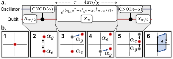
Figure M3: Geometric phase unitary to sense phase of unknown displacement (a.) Decomposition of the unitary used throughout the reservoir for time-independent tasks. (b.) Schematic representation of the dynamics of the oscillator state under the reservoir drives with time-independent input, highlighting a unitary which implements a geometric phase unitary. (1) At the start of the protocol, the qubit is in the ground state, with the cavity at vacuum. (2) An initial $X_{\pi/2}$ pulse brings the qubit to the equator. The $\mathrm{CNOD}(\alpha)$ unitary conditions the state of the cavity based on the qubit. For the first reservoir, this is a coherent state. (3) and (4) For time independent inputs, the effective action can be described by a single displacement on the cavity mode. In this experiment, we operate the displacement at a frequency which, to first order, causes a displacement only on the state conditioned on the ground state of the qubit. A qubit $\pi$ pulses switches the state in between the two displacements. (5) The final conditional displacement brings the two conditioned states back onto each other. This effectively disentangles the qubit from the cavity mode. (6) The effective geometrical area enclosed $A$, which is a function of the input, is imparted onto the qubit.

The advantage of the reservoir computing paradigm is the flexibility in the choice of dynamics. However, simple design principles, motivated by the physics of the system, can go a long way in engineering a reservoir with high expressive capacity on many tasks. In this section, we provide full details and motivations for the unitaries and measurements in this work, followed by sections outlining characterizations of the device in order to realize the intended dynamics.

The reservoir drives consists of two categories of dynamics: the unitaries and the measurements. In what follows, we will first provide analysis of the dynamics for time-independent input (e.g. the signals in Fig. 2). As we will see, the unitary component of the dynamics implemented in this work strives to implement a $\cos^{2}$ nonlinearity on the raw input, whereas the measurements generate non-classical features in the state and quantum correlations in the measurement trajectories via measurement backaction.

Whereas with a typical homodyne-setup, measuring the quadratures of some unknown signal is easy, however performing the same measurement of a displacement on an oscillator using only qubit measurements can be non-trivial. Of course, when designing a reservoir, one does not strive to implement the identity, but it is a good starting point – the unitary is thus implemented to approximate the identity. It consists of the input signal data, which is sandwiched on either side by fast conditional displacement gates implemented with CNOD [1] and qubit rotation gates. The broad-overview of the decomposed unitary is given in terms of gates in Fig. M3, along with a schematic portrayal of the phase-space trajectory of the oscillator mode initialized in vacuum subject to a time-independent drive.

We begin with an idealized gate-based version decomposition of our reservoir for time-independent input on resonance with the oscillator conditioned on the qubit being in the ground state. The sequence of gates the reservoir unitary approximates:

$$U_{1} =X_{\pi/2}$$ (19)

$$U_{2} =D(\alpha)|g\rangle\langle e|+D(-\alpha)|e\rangle\langle g|$$ CNOD (20)

$$U_{3} =D(\beta)|g\rangle\langle g|+|e\rangle\langle e|$$ Input (21)

$$U_{4} =X_{\pi}$$ (22)

$$U_{5} =U_{3}=D(\beta)|g\rangle\langle g|+|e\rangle\langle e|$$ Input (23)

$$U_{6} =D(-\alpha)|g\rangle\langle e|+D(\alpha)|e\rangle\langle g|$$ CNOD (24)

$$U_{7} =Y_{\pi/2}$$ (25)

Ignoring the very first unitary, after applying the sequence of unitaries $U_{2}$ through $U_{7}$, we arrive at unitary

$$U_{7}U_{6}U_{5}U_{4}U_{3}U_{2}=\frac{i}{\sqrt{2}}e^{\alpha\beta^{*}-\alpha^{*}\beta}D(\beta)(|g\rangle\langle g|-|e\rangle\langle g|)-\frac{i}{\sqrt{2}}e^{-\alpha\beta^{*}+\alpha^{*}\beta}D(\beta)(|g\rangle\langle e|+|e\rangle\langle e|)$$ (26)

Let

$$|\psi\rangle=[e^{-i\phi/2}\cos(\theta/2)|g\rangle+e^{i\phi/2}\sin(\theta/2)|e\rangle]\otimes|\mathrm{cavity}\rangle$$ (27)

be some arbitrary initialized state. Then for $\theta=\pi/2$, we have

$$U_{7}U_{6}U_{5}U_{4}U_{3}U_{2}|\psi\rangle=\frac{1}{\sqrt{2}}D(\beta)[i\sin(A-\phi/2)|g\rangle+\cos(A-\phi/2)|e\rangle]\otimes|\mathrm{cavity}\rangle,$$ (28)

where $A=2|\alpha||\beta|\sin(\delta)=i(\alpha\beta^{*}-\alpha^{*}\beta)$ is the geometric phase enclosed by the oscillator trajectory which is dependent on the phase difference $\delta$ between the known displacement $D(\alpha$), and the unknown displacement $D(\beta)$ (Fig M3b). Thus, for the proper qubit state before the application of $U_{2}\ldots U_{7}$, we are able to extract phase information of the displacement. We also note that the qubit and the oscillator are disentangled after the unitary, and that the effect of the unitary on the oscillator mode is a simple displacement.

Finally, pre-pending $U_{1}$ (Eq. 19) to the string of unitaries guarantees that we initialize our qubit state with $\theta=\pi/2$ when following a qubit measurement, independent of that measurement outcome. It also guarantees $\phi=\pi/2$ or $3\pi/2$ depending on the measurement outcome. The probability of measuring the qubit in the excited state conditioned on preparing it $e$ vs $g$ after the entire sequence is then:

$$P_{e|g}=\cos(A-\pi/4)^{2}\qquad\qquad P_{e|e}=\sin(A-\pi/4)^{2}$$ (29)

Thus, with this sequence of unitaries, we are able to extract the phase of some unknown displacement (relative to some known displacement $\alpha$) by simply measuring the qubit. While for the first run of the reservoir, the qubit will start in the ground state (up to thermal noise), after performing a parity measurement, the qubit state will depend on the previous measurement outcome. See Fig. M7 for an experimental implementation of the above results.

In principle, Eq. 29 enables us to perform the identity operation on the input $x,y$ points followed by a $\cos^{2}$ kernel. Without loss of generality, we take $\arg(\alpha)=0$, then $i(\alpha\beta^{*}-\alpha^{*}\beta)=\mathrm{Im}(\beta)=\beta_{x}$. Alternating between $\arg(\alpha)=0$ and $\arg(\alpha)=\pi/2$ allows us to extract $\cos^{2}(\vec{\beta})$ with two runs of the reservoir.

Whereas all gates besides the input (Eqs. 21 and 23) are fast and therefore insensitive to the cross-Kerr interaction, the primary deviation from the gate description occurs for the input, which can be very long. This input displacement is conditioned on the qubit being in the ground state. Therefore, in the rotating from of the qubit-oscillator system, the branch of the cavity state conditioned on the qubit being in the excited state will rotate at a frequency $\chi$, which in general will break the geometric phase construction for time-independent tasks. Therefore, we limit the exposure time of the reservoir to the input signal to be an integer multiple of $4\pi/\chi$, so that the cavity state conditioned on the qubit being in the excited state will return to the same point.

The unitary described in Eqs. 19-25 is followed by a qubit measurement, then a parity measurement $\Pi$ [3, 6] with projectors $P_{\pm}$, where

$$\Pi=(-1)^{a^{\dagger}a}\qquad\qquad P_{\pm}=\frac{1}{2}(1\pm\Pi)$$ (30)

As mentioned above, the effect of the unitary on the oscillator state for time-independent signals is simply a displacement of the input data $D(\beta)$, independent of the qubit measurement outcome. For the following discussion, we will ignore the qubit dynamics, since the qubit and the oscillator are disentangled at the end of the unitary. In effect, the state of the cavity can be described by a series of alternating displacements and parity measurements:

$$|\mathrm{cavity}\rangle=\ldots P_{p_{4}}D(\beta)P_{p_{3}}D(\beta)P_{p_{2}}D(\beta)P_{p_{1}}D(\beta)|0\rangle,$$ (31)

where $P_{p_{n}}$ is the projector of the $n$th parity measurement with outcomes $p_{n}=\{+,-\}$. For $k$ runs of the reservoir, we can reorder terms and add pairs of canceling displacements $D(-\beta)D(\beta)$ to rewrite the above as

$$|\mathrm{cavity}\rangle=\left(\prod_{n}^{k}P_{p_{n}}^{n\beta}\right)D(k\beta)|0\rangle.$$ (32)

Equation 32 describes a series of projective measurements after preparing a displaced vaccum state. The projectors and their associated measurements are

$$P_{\pm}^{\alpha}=D(\alpha)P_{\pm}D(-\alpha)\qquad\qquad\Pi^{\alpha}=D(\alpha)\Pi D(-\alpha)$$ (33)

The measurements $\Pi^{\alpha}$ describe parity measurements in displaced frame at $\alpha$. Incidentally, the expectation value of this operator are proportional to the Wigner function at $\alpha$ [Royer1977]. However, importantly, Eq. 32 does not describe performing Wigner tomography of the state $D(k\beta)|0\rangle=|k\beta\rangle$ at points given by $\beta,2\beta,3\beta,\ldots$, as the effective measurements $\Pi^{\alpha}$ do not commute for different values of $\alpha$. Instead, in general $[\Pi^{\alpha},\Pi^{\gamma}]\neq 0$. Therefore, in this light, our reservoir construction can be seen to leverage non-commuting measurements and quantum contexuality to generate conditional and correlated probabilities over measurement trajectories.

Reservoir description for slow varying time-dependent signals

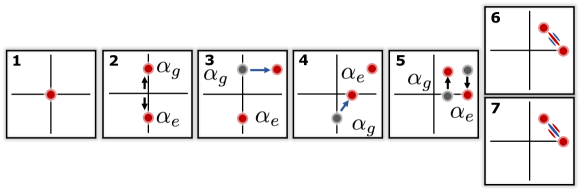
Figure M4: Schematic description of the dynamics of the oscillator, starting in vacuum, for a slow time-varying input In such a scenario (as is the case for the task of classifying radio modulation schemes), the signal causes a displacement largely conditioned on the ground state. Generally, the value of the displacement is different before and after the $\pi$ pulse in between (3) and (4). Unlike the regime for time-independent signals, there is no effective area enclosed in phase space, which leaves the qubit entangled with the cavity. (6) and (7) describe the state of the cavity after the qubit measurement. The resulting state of the cavity is a cat state, where the parity of the cat dependent on whether the outcome of the qubit measurement is ground or excited.

For generic, time-dependent signals, like those classified in Figs. 3 and 4 in the main text, the geometric unitary described by Eqs. 19-25 does not in general hold, as the symmetry between panels 3 and 4 in Fig. M3 is broken. Additionally, the approximation that the input is displacement conditioned on the qubit in the ground state (Eq. 21 and 23) will not hold for high bandwidth signals, like those in Fig. 4 in the main text. For high-bandwidth signals, the input will also have some contribution in displacing cavity state conditioned on the qubit being in the excited state, which can lead to complex dynamics in the cavity state. While for generic signals, this can be hard to describe, here we prove a treatment of our reservoir construction for slowly-varying, time-dependent signals, like those in Fig. 3 of the main text.

We can follow most of the derivation from the scenario of time independent signals in Appendix C, to describe the dynamics of the QRC for the task of classifying radio frequency modulation schemes. Along with the assumptions in the previous section, we make the slow-varying input approximation, such that the displacement on the oscillator of the reservoir is still effectively conditioned on the ground state of the qubit. The displacement on the cavity depends on the value of the symbol encoded for the given modulation scheme. Since, in general, the symbol is different before and after the qubit $\pi$ pulse: the direction of the displacement in the cavity will be different. Given the timescales of the input signal involved, this essentially corresponds to a displacement on the cavity state conditioned on the ground state of the qubit. When the two displacements are different in magnitude and direction, the qubit remains entangled with the cavity at the end of the reservoir unitary. The state of the system just before the measurements is (step (5) of Fig M4:

$$|\psi\rangle=\frac{1}{\sqrt{2}}(e^{-iA_{i}}D(\beta_{i})|g,\mathrm{cavity}\rangle+e^{iA_{j}}D(\beta_{j})|e,\mathrm{cavity}\rangle),$$ (34)

where $\beta_{i}$ is the displacement before the qubit flip, and $\beta_{j}$ is the displacement after. $A_{i}=\alpha\beta_{i}$ is the phase acquired after two non-orthogonal displacements. When $\beta_{i}=\beta_{j}$, we recover the dynamics for time independent signals. It is straightforward to show that the qubit will be disentangled from the cavity and that the area $A_{i}$, corresponding to the geometrical phase form the area enclosed in phase space will be present as a relative phase difference between the ground and excited state. After a $Y_{\pi/2}$ gate, we have the following state in our system:

$$|\psi\rangle=\frac{1}{2}[e^{iA_{i}}D(\beta_{i})+e^{-iA_{j}}D(\beta_{j})]\otimes|g,\mathrm{cavity}\rangle+\frac{1}{2}[e^{iA_{i}}D(\beta_{i})-e^{-iA_{j}}D(\beta_{j})]\otimes|e,\mathrm{cavity}\rangle,$$ (35)

One can think of this as a cat state in the cavity, with a parity determined by the qubit state. This is schematically shown in (6) and (7) in Fig M4. In the limit of very different displacements, the probability of the qubit measurement is the same for both ground and excited states. The goal of this task can be thought of as discriminating probability distribution functions over the $(I,Q)$ plane. Fig 3 (a) represents the so-called “constellation ” diagram of the modulation schemes considered in this work. Each scheme can take discrete values in $(I,Q)$ space, with even equal probability (we construct the dataset of radio signals encoding random binary strings). Our lack of knowledge of the exact displacement on the cavity can be mathematically expressed as a density matrix. This is the most apparent in the state of the cavity after the initial qubit measurement,

$$\rho_{\mathrm{cavity}}^{\prime}=\sum_{\beta_{i}\in P}p_{i}D^{\dagger}(\beta_{i})\rho_{\mathrm{cavity}}D(\beta_{i})+\sum_{\beta_{i},\beta_{j}\in P}p_{ij}e^{i(A_{i}-A_{j})}D^{\dagger}(\beta_{i})\rho_{\mathrm{cavity}}D(\beta_{j}),$$ (36)

where $\rho_{\mathrm{cavity}}^{\prime}$ is the density matrix representation of the cavity right after the qubit measurement and $\rho_{\mathrm{cavity}}$ describes the initial density matrix before the application of the input. The set $P$ describes the distribution of possible displacements which can be received from the input. $p_{i}$ is probability for receiving the symbol corresponding to a displacement $\beta_{i}$, and $p_{ij}$ is the conditional probability of displacement $\beta_{j}$, given $\beta_{i}$. For the task considered in this work, these distributions are uniform, with no contributions from conditional probabilities. However, this description of the reservoir motivates the potential for the QRC to distinguish signals with complex correlations in the symbols of the message encoded.

Appendix D Quantum reservoir characterization

CNOD

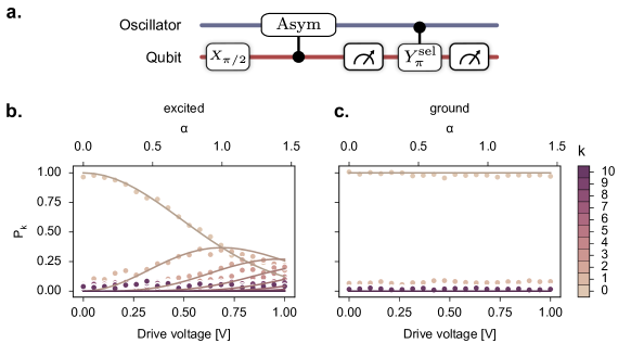
Figure M5: Characterization of conditional displacements using an Anti-symmetric pulse from Ref. [1]. (a.) Pulse control schematic of characterization of conditional displacement. Here, we make use of number-splitting spectroscopy to characterize the state of the cavity after perform a conditional displacement on the state $|+\rangle|\mathrm{vacuum}\rangle$ conditioned on the qubit state. By post-selecting on the qubit state, we can evaluate the effectiveness of the conditional displacement. (b.) Number splitting spectroscopy conditioned on measuring the qubit in the excited state. A single parameter fit is used to capture the behavior of the state of the cavity as a function of amplitude. From the good agreement, we conclude that conditioned on measuring the qubit in the excited state, the cavity is displaced. (c.) Number splitting spectroscopy conditioned on measuring the qubit in the ground state. We see very limited change in the cavity state when measuring the qubit in the ground state.

Here, we provide the calibration of the CNOD unitary [1], one of the components of our reservoir unitary (Fig. M3). The CNOD protocol implements the following unitary

$$\mathrm{CNOD}(\alpha)=D(\alpha)|g\rangle\langle e|+D(-\alpha)|e\rangle\langle g|.$$ (37)

The protocol is implemented with two ‘Anti-symmetric pulses’ sandwiching a qubit pi-pulse. In the frequency domain, the pulse is composed of two gaussian envelopes offset such that there is a zero-crossing at the qubit ground state frequency, and that the spectrum is anti-symmetric around this point (see Ref. [1]). The Anti-symmetric pulse is a conditional displacement, conditioned on the qubit being in the excited state. The motivation for using CNOD instead of a single tone displacement on resonance with the stark-shifted qubit frequency is that it enables the ability to perform conditional displacements at time scales much smaller than $2\pi/\chi$.

Figure M5a displays the protocol for characterizing the anti-symmetric pulse. First, the qubit is unconditionally brought to the equator of the bloch sphere, with a wide-band $X_{\pi/2}$ pulse. After this, the anti-symmetric pulse acts on the cavity, followed by an qubit measurement, collapsing the cavity state to either $D(\alpha)|0\rangle$ or $|0\rangle$. After collapsing the state, we perform a number-splitting spectroscopy on the cavity. This is performed with a conditional $Y_{\pi}$, conditioned on the $k$th cavity Fock state [Gambetta2006, Schuster2007] followed by a second qubit measurement. By post-selecting on the first qubit measurement outcome, we can characterize the cavity state for each branch. Figure M5b and c show the number-splitting spectroscopy for the cavity state conditioned on the qubit being in the ground state vs excited, as a function of pulse amplitude. These curves are fitted with a single parameter scaling parameter that defines the relationship between pulse amplitude voltage and the amount of displacement $\alpha$.

Reservoir unitary characterization

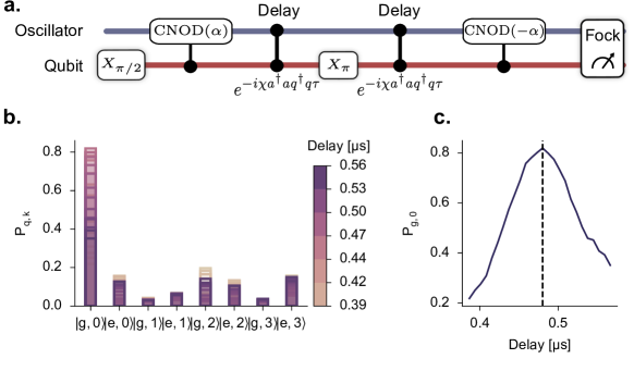
Figure M6: Characterization of input signal duration (a.) Diagram of control sequence to calibrate length of input signal duration toward implementing the geometric phase unitary in Eqs. 19-25. Here, a double conditional displacement is performed after sending the qubit to the equator of the Bloch sphere. After this, a variable delay is added before undoing that displacement. Finally, the qubit and the Fock distribution of the cavity is sampled using methods from Refs. [6, deng2023heisenberglimited]. (b.) Overlapping histograms showing Fock distribution of cavity state conditioned on qubit state as a function of delay. (c.) Cavity state overlap with the vacuum state as a function of delay. At a particular value of the delay, the two displacements interfere and cancel each other out.

With our rotation gates and CNOD’s calibrated, we describe in this section the calibration of signal drives toward the implementation of Eqs. 19-25. We begin with a calibrating the duration of time our reservoir is exposed to the input signal. As discussed in Appendix C, calibrating this delay is crucial for a faithful implementation of the geometric phase detection unitary introduced in this work. While it may seem that this restriction in the signal duration is contrived and unrealistic in a real-world setting where the signal is unknown, we argue we can get around this by putting a commercial fast switch.

Figure M6a schematically describes the experimental protocol for calculating the delay between the two CNOD pulses. Here, we effectively try to undo a double conditional displacement via second double conditional displacement. Due to the dispersive shift, after the first conditional displacement, the state of the cavity conditioned on the excited state of the qubit will start rotating with respect to the state of the cavity conditioned on the ground state. After a period of $2\pi/\chi$, the this will return to the same position as the start. Undoing the displacement at this point in time will send the cavity state to vacuum. Figure M6b shows the fock distribution of the cavity as a function of the waiting time, and Fig. M6c shows the cavity state overlap with the vacuum state as a function of the waiting time.

Figure M7: Full geometric phase unitary calibration. (a.) Pulse control protocol for the unitary defined by Eqs 19-25. This protocol is identical to that of Fig. M3a. (b.) Overlapping histograms showing the probability over outcomes of measuring the qubit and oscillator-parity as a function of the phase of the input signal with $|\beta|=0.25$. As the phase is varied, the probability of the qubit being excited increases. (c.) The probability of measuring the qubit excited as the phase of the input displacement $\beta$ is varied, plotted for different values of $|\beta|$

Next, we implement the full unitary given by Eqs. 19-25, where the section corresponding to the input data displacement (Eqs. 21 and 23) is given by the duration found in the results above. For this calibration, we implement the full unitary given by the diagram in Fig. M3a by varying the angle of the input displacement and looking at the dependence.

Figure M7a shows the schematic overview of the calibration procedure. The geometric phase unitary is parameterized by a long displacement, whose angle we sweep. After the unitary we perform a qubit measurement, followed by a parity measurement. This calibration experiment is essentially identical to the time-independent reservoir computing experiments in terms of the control protocol. Here, instead of sending data from different distributions for the system to classify, we only vary the phase and amplitude of some input displacement so if we get the phase dependence we want.

Figure M7b shows the distribution of measurement outcomes from measuring the qubit and the oscillator parity after the unitary is applied with $\alpha=1$ and $\beta=0.25$. As the angle of the input is swept, the qubit probability of the qubit being in found in the ground state shifts to being found in the excited state. This is more evident in Fig.M7c where we plot the probability of measuring the qubit in the excited state $P_{e}$ as a function of the phase of $\beta$ for different amplitudes of $\beta$. In comparison we find great qualitative agreement with the expected result $P_{e}=\cos(2|\alpha||\beta|\cos(\delta)+\pi/4)^{2}$, where $\delta=\arg(\alpha)-\arg(\beta)$ (see Eq.29), though we find an extra reduction in the dynamic range in $P_{e}$ for increasing $\beta$ due to qubit overheating.

For our quantum reservoir tasks, we choose $\alpha$ to be quite small, near 0.2. The effect of this is a severe reduction in the dynamic range of $P_{e}$, but one that is easily distinguishable at 1000 shots. For all of our tasks, this was the mininum number of shots needed to get 100%. Keeping $|\alpha|$ small allows for a greater sensitivity in $|\beta|$ without worrying about qubit overheating.

Qubit & parity measurements

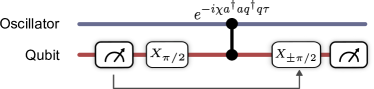
Figure M8: Qubit and oscillator-parity measurements in the quantum reservoir computer. For our reservoir construction, the state of the qubit is not generally known before a parity measurement. We apply feedback to change the parity measurement based on the preceding qubit measurement to faithfully capture the oscillator parity.

The qubit and parity measurements performed in this work are the standard pulse schemes used in many previous works, with one change. The typical procedure of measuring the parity of a cavity state is similar to a Ramsey experiment (and perhaps more closer still to a ‘qubit-revival’ experiment [chou2018teleported]), and importantly requires knowledge of the state of the qubit before the measurement is performed. In a quantum reservoir setting where measurement trajectories can be unknown, measuring the parity of the cavity is not straight-forward without post-selection or feedback. Here, since we perform a qubit measurement just before the parity measurement, we apply simple feedback that conditions the parity unitary on the measurement outcome of the preceding qubit measurement. The condition is such that the parity measurement outcome is now independent of the preceding measurement outcome. This reduces the order of correlations required to gain the same information: attaining the parity of the cavity only requires information about the parity measurement, whereas previously, second order correlations between the qubit and parity measurement was required. A further refinement to reduce trivial correlations in the measurement history would reset the qubit after the oscillator parity, however, due to limitations in the FPGA software, this was not implemented.

Tuning $T_{2}$ via resonator-induced dephasing

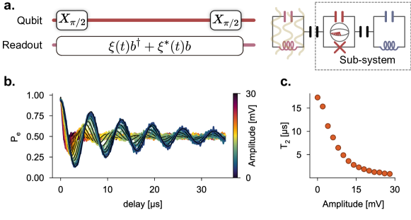
Figure M9: Resonator-induced dephasing via pumping on the readout resonator (a.) Protocol for characterizing the effect of a readout pump on qubit decoherence: we perform a typically Ramsey experiment while populating the readout resonator to measure the $T_{2}$. (b.) Ramsey curves as a function of readout pump amplitude. These curves are fit using Eq. 38 to produce estimates of the qubit coherence. (c.) Extracted $T_{2}$ values for each of the curves in part (b)

Here we describe the experiment to reduce the qubit coherence time by pumping the readout resonator with photons during our reservoir experiments (see Fig. 2d). The calibration of this experiment involves performing standard a Ramsey $T_{2}$ experiment, modified with a pump on the readout resonator (Fig. M9a). Once populated, the resonator photons induce an dispersive shift, which, sends the qubit to the center of the Bloch sphere once the readout resonator is traced out. In principle, this interaction is coherent, and the qubit should see a revival; however, due to the leaky nature of the readout resonator by design, a coherent revival is not observed. As remarked in the end of Appendix B, this experiment required an auxilliary AWG line. Figure M1 denotes this as the ‘Readout Auxillary’ line.

Figure M9b shows the results of the Ramsey calibration with the readout pump on, for varying pump powers. We see a steady decrease in the qubit coherence time as the pump amplitude is increased as expected. The curves are fit to the equation

$$P_{e}=\cos(2\pi\delta t)e^{-t/T_{2}},$$ (38)

where $\delta$ is an intentional detuning. Here, a Gaussian pulse was used as the readout pump. We expect that due to the construction of the reservoir, a flattop pulse may be more detrimental to the classification performance, since the Gaussian pulse has little amplitude during the CNOD unitaries shown in Fig. M3a. Finally, we note that the maximum $T_{2}$ shown in Fig. M9 differs from the value quoted in Table S1. After preliminary calibration data corresponding to those in Fig. M9, the experiments in Fig. 2c were performed, after which the qubit $T_{2}$ was suddenly lowered. However, all experiments presented in this manuscript, with the exception of Fig. M9, were performed where the qubit $T_{2}$ matched that of Table S1. Given the conclusion that the qubit $T_{2}$ did not impact classification accuracies until it approaches the time between measurements, we decided to include the higher quality data presented in Fig. M9, rather than the preliminary data used to calibrate the results in Fig. 2c.

Appendix E Machine learning with the quantum reservoir

Output feature encoding

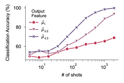
Figure M10: Comparison of feature vectors in spiral classification performance Here, classification accuracy on the spiral task is considered for different output encodings. Particularly, we compare included higher and higher correlations. $\vec{\mu}_{\leq p}$ describes a feature vector containing all central moments up to and including the $p$-th central moment (see text).

In this work, we use measurement correlations as the output feature vectors from which the trained linear layer of our reservoir performs the classification. In this section, we provide details in how these were constructed from measurement results, as well as motivations and comparisons with other output encodings. As described in the main text, measurements of our reservoir involve two measurements following every data input: a qubit measurement and a parity measurement. The qubit measurement, which follows just after the input unitary, either extracts information about the input displacement (if the signal is time-independent), or performs some nontrivial back-action on the oscillator state (see Fig. M4). The parity measurement, which follows the qubit measurement, will simply measure the parity of the cavity state post-qubit measurement, and collapse the oscillator state to either even or odd Fock states. It is worth pointing out that measurements of the parity are done with an entangling unitary starting with a known qubit state and then performing a regular qubit measurement (see Appendix D for details).

In this manuscript, qubit measurements are performed using standard dispersive readout, which we review here, since the process involves a number of nonlinear steps (for a thorough review, see Ref. [Blais_2021]). Each measurement outcome is the result of integrating a response signal from the readout resonator, and is defined by a single point on the $I-Q$ plane. For sufficiently strong coupling between the readout resonator and the qubit compared with the resonator linewidth, the set of all possible integrated IQ points will form two (or more) localized and well-seperated blobs, indicating projective measurement with single-shot fidelity. These two (or more) blobs correspond to different states of the transmon, and single-shot fidelity refers to the ability to discern the state of the qubit using only one readout pulse. With knowledge of the location of these blobs, and which state they correspond to, we perform a threshold the measurement result to either ‘0’ or ‘1’, indicating the qubit ground state or excited state respectively.

From a string of binary measurement outcomes, or bitstring, we form our feature vectors by first calculating the $p$-th central moment $\mu_{p}$, defined as

$$(\mu_{p})_{ijkl\ldots}=\frac{1}{N_{\mathrm{shots}}}\sum_{n}^{\mathrm{N_{shots}}}(x_{ni}-\langle x_{i}\rangle)(x_{nj}-\langle x_{j}\rangle)(x_{nk}-\langle x_{k}\rangle)(x_{nl}-\langle x_{l}\rangle)\ldots,$$ (39)

where the number of indices of $\mu_{p}$ is equal to $p$. Here $x_{ni}$ is the $n$th repeated measurement result of observable $x$ labeled by $i$. In our setting, $i$ labels the $i$-th measurement in a sequence of correlated measurements before the system is reset. The expectation value $\langle x_{i}\rangle$ is taken over the shots $N_{\mathrm{shots}}$ – counting the number of system resets and repetitions. Faithful estimates of these moments are made with enough shots typically requiring on the order of a 1000 shots for the results presented in this manuscript.

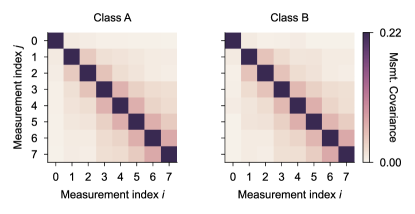
Figure M11: Second-order central moment (covariance) of quantum reservoir output over spiral dataset. These correlation matrices were generated from calculating the covariance over measurement outcomes in a reservoir run, then averaged over the entire dataset.

The central moments of Eq. 39 are used in the construction of the output feature vector for the linear layer to perform the classification task. Specifically, the feature vector is generated by appending successively more and more central moments. We denote these appended feature vectors as $\vec{\mu}_{\leq p}$ for feature vectors containing up to $p$ central moments, e.g. $\vec{\mu}_{\leq 2}=[\vec{\mu}_{1},\mu_{2}]$ is a feature vector constructed from appending the covariance to the mean. The first order moment here is a vector to denote that the mean is taken over repetitions of different measurements, whereas the covariance is a matrix and thus is not denoted as a vector. Additionally, we only take the upper triangle of the covariance at most, since that contains all the independent degrees of freedom of the symmetric covariance matrix.

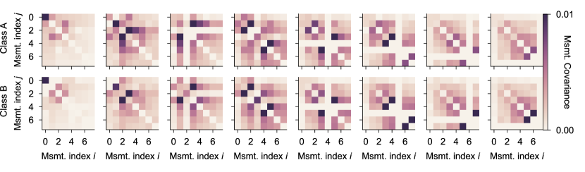
Figure M12: Third-order central moment of quantum reservoir output over spiral dataset. These third-order central moments are plotted as an array of 2D matrices, such that the $i$-th column corresponds to the 2D matrix $\mu_{ijk}$. The two rows corresponds to the two different classes of signals. In the third order, one can begin to see differences between the two classes by eye.

Figure M10 contains classification results on the spiral dataset (Fig. 2) as a function of the number of shots for the feature vectors $\vec{\mu}_{1},\vec{\mu}_{\leq 2}$ and $\vec{\mu}_{\leq 3}$. We see that our quantum reservoir has non-trivial third-order correlations and that the reservoir leverages these correlations to boost classification accuracy. The covariance matrix averaged over the entire spiral dataset is plotted in Fig. M11, and the third order correlations are plotted in Fig. M12 – plotted as a set of 2D matrices. In the third-order correlations in particular, we can begin to pick out by eye the differences in the two classes.

In general, for arbitrary moments, the number of independent components is ${M+p-1}\choose{p}$, where $p$ is the order of the moment, and $M$ is the number of measurements. This construction generally allows us to construct feature vectors that are smaller than the sample probability over all possible measurement trajectories, which is $2^{M}$ dimensional. However, as can be seen in Fig. M11, there is yet redundant information even after taking only the symmetric part, specifically, that the information tends to be very local and that measurements far apart tend not to be correlated. This has the physical interpretation that while measurements are indeed correlated, even possessing higher-order correlations, this correlation tends to be local due to the finite memory of the system. This motivates us to further restrict our feature vector to only capture the essential local correlations.

Figure M13 compares the classification performance of feature vectors generated with up to third-order moments, where we truncate the locality of the correlations. That is, the elements of the third order central moment $(\mu_{3})_{ijk}$ is set to zero if $|i-j|>d_{H}$ or $|i-k|>d_{H}$, for some integer $d_{H}$ we interpret as a Hamming distance. We note that including third-order correlations between measurements that are up to three ‘sites’ away nearly reproduces the classification accuracy of when you include all third-order central moments. Additionally, we compare the construction of feature vectors using truncated moments up to third-order with that of using the full sampled distribution as the feature vector. These last two statements were found to be true for all tasks presented in this paper. We used the truncated third-order correlations as the feature vector as the universal feature vector for all tasks presented.

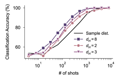
Figure M13: Spiral classification accuracy as a function of locality of up-to third order correlations Classification accuracy for the spiral task using up to third-order central moments truncating correlations to only include correlations up to $d_{H}$. We find that we can achieve high accuracy using local third-order correlations, saturating the accuracy when only keeping correlators up to $d_{H}\leq 3$. The performance of using the sample distribution is also compared which performs worse than using the central moments as output features, despite containing more information (see text).

Training the linear layer

The only component of the reservoir that was trained to fit the dataset processed by the reservoir was the linear layer applied to the feature that the physical reservoir produced. The linear layer was an $R\times C$ matrix $W_{\text{train}}$ and $C$-dimensional vector $v_{\text{train}}$ applied to the $R$-dimensional reservoir feature $x$ to get

$$y=W_{\text{train}}x+v_{\text{train}}$$ (40)

where the largest of the $C$ elements of $y$ corresponded to the predicted class of the data point ($C$ is the number of classes). To train the linear layer, we chose between two different approaches: the pseudo-inverse method and back-propagation through a softmax function on the output.

First, we will describe the pseudo-inverse method. Let $X$ be a $N\times(R+1)$ matrix consisting of $R$-dimensional reservoir features generated for $N$ training points, with a row of 1’s appended (this is to compute both $W_{\text{train}}$ and $v_{\text{train}}$ at once). Let $Y$ be an $N\times C$ matrix consisting of $C-$dimensional column vectors that serve as labels for the training points such that $Y_{i,j}=1$ if $j$ corresponds to the class of the $i^{\text{th}}$ training point and zero otherwise. For an $\epsilon>0$, we construct $W^{{}^{\prime}}_{\text{train}}$ ($W_{\text{train}}$ appended with $v_{\text{train}}$) as :

$$W^{{}^{\prime}}_{\text{train}}=\left(X^{T}X+\epsilon I\right)^{-1}X^{T}Y$$ (41)

In our case, the value of $\epsilon$ was swept to maximize the accuracy of the classification. In the limit of $\epsilon\rightarrow 0$, pseudo-inverse matrix of Eq. 41 minimizes the mean squared error between $XW_{\text{train}}$ and $Y$, and so has been a popular choice for training the linear layer at the output of reservoirs [nakajima2018reservoir, LESNREVIEW2022, 2, scardapane2017]. However, our goal was to classify the input signals based on the largest element of the final output vector. Consequently, the linear layer that resulted in the lowest mean squared error with our labels was not always the linear layer that gave us the best accuracy.

For this reason, we also used a second training method for our linear layer. This approach used softmax and back-propagation using the automatic differentiation package from PyTorch [pytorch2019]. In this approach, the prediction vector $y$ from Eq. 40 is passed through the “Softmax” activation function:

$$(y_{\text{prediction}})_{i}=\frac{\exp(y_{i})}{\sum_{j=1}^{C}\exp(y_{j})}$$ (42)

We then computed the mean squared error between the resulting $y_{\text{prediction}}$ and label for the training point that produced the underlying reservoir feature, and used back-propagation to compute the gradient for our linear layer. The linear layer was then updated using the ADAM optimizer [ADAMpaper] with the default settings of $\beta_{1}=0.9,\beta_{2}=0.999$ and a learning rate of $0.01$. For our reservoirs, we tried both methods of training the linear layer and used whichever yielded the best accuracies. Empirically, we found that while pseudo-inverse training was better in some cases, training the linear layer with back-propagation often yielded quite large accuracy advantages over pseudo-inverse.

Appendix F Supplementary information machine learning tasks

Classification of Radio-Frequency signals

In this section, we discuss about the algorithm for generating the dataset for the classification of digital modulation schemes on radio signals. The digital modulation scheme involves encoding sequences of binary values into the amplitude and phase of a radio signal for a fixed duration. The number of binary values encoded depends on the modulation scheme. For example, for BPSK (binary phase shift key), each symbol (change in property of the signal) encodes one bit of information. For $32$QAM (quadrature amplitude key), there are $32$ possible values, which allows each symbol to contain $5$ bits of information. For this task, we keep the symbol rate fixed across all the tasks. Moreover, the pulses generated by the arbitrary waveform generator (AWG) all occur at the baseband frequency. This signal is then upconverted to the frequency of the cavity before sent to the device. To generate the set of possible sequences, we randomly select each symbol with equal probability. This corresponds to the case of each possible binary string of digits encoded to be equally likely. Due to memory constraints on the AWG, we cannot output a continuous encoded signal for long durations, corresponding to the regime of large samples of the reservoir. We circumvent this constraint by realizing that, for this task, there are no correlations in the encoded binary digit sequence (since each symbol is equally likely). Therefore, for example, the probability of a long binary digit sequence can be correctly emulated by sampling multiple short binary digit sequences and concatenating them together. For this task, we can simply achieve this by generating a signal with eight symbols, which is the number of symbols enter our QRC before its state is completely reset.

Classification of noisy signals

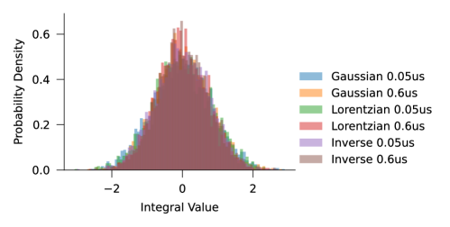
Figure M14: Histogram of integrated value of the input signal for the noise classification task. In this work, we enforced a normalization condition on the amplitude of the filter functions. We set the normalization such that the long time integral of the signal corresponds to a value with zero mean and the same standard deviation. This is visually seen from the probability density function from the dataset of the classes of noisy signals. We do this to ensure that any reservoir which simply integrated the signal, before applying a non linear kernel, cannot classify the different signals. The fact that our reservoir is able to solve this task can therefore be associated with the continuous-time processing by the cross-Kerr interaction between the oscillator the cavity. Enforcing this normalization is mathematically equivalent to setting the DC component of the filter functions to be the same value in frequency space.

To generate the dataset describing the task of classifying noisy signals using the QRC (see Fig. 4), we start with emulating white noise. At each time step of the sampling rate of the AWG, we choose a value for in-phase and quadrature signals uniformly between the unit interval (up to an overall normalization). While this is limited to the sampling rate of the AWG (around $2\times 10^{9}$ samples per second), this is much larger than any relevant time scale of the experiment. Therefore the approximation of broadband white noise is appropriate to describe the effect of the signal on the system. We then apply “kernels” as a convolution in the time domain to each need seed of the white noise generated signal. This can also be thought of a bandpass filtering function in frequency domain. The classification task is then to identify the kernel. Each kernel is defined by a time domain function. The only hyper-parameter to describe each kernel is the overall scaling value. In this work, we set the DC component of this kernel in frequency domain to be the same for all classes (set to unit value without loss of generality). In the time domain, this corresponds to scaling the amplitude such that the area enclosed by the filter function in time is the same for all functions.. We do this to make sure that a direct integration of the signal over a time domain much longer than the correlation length introduced by the kernel, cannot distinguish the signals from each (see Fig. M14). The above normalization ensures the random variable associated with the value of this integrated value is the same for all distributions. Therefore, this ensures that any ability of the reservoir to classify the signals is intrinsically from its computational capacity to distinguish short-time correlations (in this work we choose a correlation time scale of $50$ns and $600$ns, with kernel functions of Gaussian, Lorentzian, and the Inverse function: generating a total of $6$ classes.).

Appendix G Simulation of the quantum reservoir

Introduction

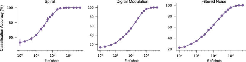
Figure M15: Classification accuracies obtained from numerical simulations of the QRC. Numerical simulations of the quantum reservoir can help guide the expected performance of the system in experiment. Here, we simulate the three main tasks considered in the paper: Spiral (a time independent input with the goal of classifying the arms of the spiral), Digital Modulation (a slow varying time dependent signal with the goal of identifying the digital modulation scheme used in the signal), Correlated Noise (a fast varying time dependent signal with the goal of classifying the “kernel” of correlation function).

Classical simulations of the QRC can provide insight into the expected computational capacity in experiment. For our work, classical simulations of the dynamics of the reservoir were primarily performed with the aid of QuTiP [4]. The algorithm to estimate the classification accuracy for a given task then follows the same technique used in experiment, with training and testing datasets on the measurement outcomes of the simulation. We implement the Hamiltonian in Eq 1, by approximating the transmon as a qubit, and introducing a finite dimensional Fock truncation to the cavity subspace. It is important to ensure that the Fock truncation does not introduce any spurious effects, for it can be a source of non-physical non-linearities in the system. For example, a linear cavity, treated as a harmonic oscillator, only performs a linear transformation on an incoming analog radio frequency signal. However, if in simulation, the support of the state of the cavity exceeds the Fock truncation of the simulation, numerical errors introduce non-gaussian states in the cavity mode. Such effects will depend non-linearly on the input, and hence can effectively act as a “good” (but of course unphysical) reservoir! To ensure this doesn’t happen in simulation, at every step of the unitary evolution, we monitor the probability of the wavefunction on the largest Fock state in the simulation. If this value goes above $1\%$ during the simulation, a warning is raised, and the results of the simulations are discarded.

To make the simulations efficient, we make certain assumptions on the quantum system. Firstly, we treat the reservoir controls of qubit rotations and conditional displacements with a “gate”-based unitary. However, to take into account the analog, continuous dynamical evolution implemented by the cross-Kerr interaction term in the Hamiltonian, the interval of the input into the system is implemeted with the full time-dependent Hamiltonian evolution (using QuTiP’s “mesolve” functions). Finally, another approximation we make (in favor for simulation speed) is ignoring decoherence effects. To ensure this approximation is valid, we performed simulation with the stochastic wavefunction approach with photon loss and qubit dephasing rates measured in experiments [PhysRevLett.68.580]. We obtain differences in expected classification accuracies within error bars (which are obtained from different datasets from repeated simulations). This also gives us confidence that the role of decoherence in the system plays a minimal role in the computational capacity of the reservoir. The results of the simulations with the third central moment are plotted in Fig. M15. Interestingly, the performance as a function of the number of samples agrees to experiment within the same order of magnitude. This gives a good estimate for the experimental time required for produce a classification accuracy versus shots curves in experiments. For all the three tasks, the reservoir approaches $100\%$ with sufficient samples or integration time of the input.

The advantage of continuous-time continuous-variable QRCs over discrete-time qubit-based QRCs

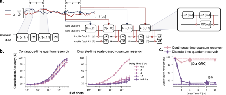
Figure M16: Simulations comparing the performance of a continuous-time quantum reservoir (our work), and a discrete-time qubit-based quantum reservoir, based on a recently implemented protocol [7]. (a.) Schematic reservoir protocol for our experiment (on the left), versus that introduced in  [7], involving two qubits as the data qubits, and two as the ancillas. The reservoir consists of single qubit rotations interleaved with CNOT gates between the data qubits and data and ancilla qubits. In this simulation, we simulate the performance of the two reservoirs as a function of the delay $\tau$ between two durations of the input. Such a delay can be introduced by the finite pulse durations and latencies introduced by the FPGA. (b.) Classification accuracy cueves for the two reservoirs as a function of shots, for different values of delays. The continuous time analog reservoir is much more robust to delays between inputs compared to the discrete time reservoir implementation. (c.) Plot of accuracies at $5000$ shots for the two reservoir implementations as a function of delay time. Experimentally relevant times include $4\mu s$ for our experiment, and around $8\mu s$ [hua2023exploiting] for the experimental realization of [7] on an IBM quantum computer.

In this section, we benchmark the performance of our continuous-time-continuous variable QRC in comparison with other hardware implementations of reservoirs. To highlight the benefit of our QRC in processing time varying input signal, we compare the simulation of our reservoir with that of a recent QRC scheme involving repeated measurements on a multi-qubit based superconducting circuit quantum system [7]. For this comparison, we simulate the expected performance of both systems on the task of classifying different noise signals with the classes described in Fig. 4. While our reservoir can naturally interface with analog signal, this is not the case with the protocol introduced in [7]. For this simulation, the signal is samples at discrete time and input to the system as a scalar parameter (one for the in-phase value and one for quadrature value). To highlight the advantage of our QRC, we slightly modify the task introduced in the Fig. 4. Here, we normalize the six filter functions such that the integral of the filter function in frequency domain is kept constant. We do this such that the standard deviation associated with the distribution of the sampled signal is the same across all signals. The only information distinguishing amongst the signals is in the correlation between two close samples in time. To elucidate this reasoning, we simulation the performance of the two reservoirs as a function of the time duration in between two samples of the signal (in the case of the discrete qubit based reservoir) and integration windows (for our analog reservoir). Such a finite duration can arise from finite-pulse durations of reservoir protocols, qubit-measurement times, and the finite latency introduced by the classical FPGA processor. For example, for our experiment, this time is around $4\mu s$, mostly arising from the measurement of the qubit and the parity of the cavity. In experiment (Fig. 4), we had generated and timed the input wave forms such that the delay between inputs is essentially $0\mu s$. For a typical IBM quantum device with mid-circuit measurement, the protocol used in Ref. [7], the finite latency can be estimated to be around $8\mu s$ [hua2023exploiting]. The protocol for the discrete-time quantum reservoir is designed to only act on real values input signals. However, for a continuous signal in the rotating frame, we have both the in-phase and quadrature values. For the experimental quadrature, these values correspond to displacements on the oscillator in orthogonal directions. To extend the scheme presented in [7], we do the following minimal change: we interleave the between sample points of in-phase and quadrature values. We could have chosen these points with the delay of $\tau$ in between each. However, this might have the effect of introducing twice the delay compared to the continuous time reservoir. Therefore, we choose the relaxed constraint of the input such that both the in-phase and quadrature values are chosen at the same point, with just a delay in between two different in-phase and quadrature points.

Comparison to other reservoirs

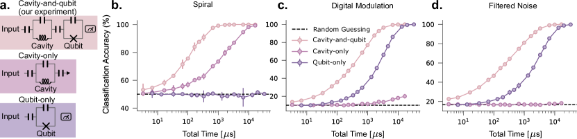
Figure M17: Simulations of the performance of the cavity-and-qubit reservoir system with its components: just a cavity reservoir and just a qubit reservoir. (a.) The circuit diagrams of the three quantum reservoir simulated here. 1) The circuit diagram of the experimental QRC in this work: a cavity coupled to a qubit. The input is interfaced to the cavity, and the state of the qubit is measured using the standard dispersive readout technique with a readout resonator. 2) The circuit diagram of a cavity as a reservoir. In this case, the natural output of the cavity is the transmitted signal. 3) The circuit diagram of a qubit reservoir. In this case the input is coupled instead to the qubit. (b.) Simulation of the classification accuracy of the three different reservoirs for the three tasks considered in the paper. As a fair comparison, the output feature vector dimension is kept constant for all three reservoir. The experimental setup drastically outperforms either of its components, just a cavity (in (c.) and just a qubit (in (d.)), which highlights the important role of entanglement in classification accuracy.

A cavity coupled to a qubit is a hardware efficient quantum system to perform reservoir computing on analog signals. In this section, we motivate this by simulating the performance of other natural choices of quantum reservoirs: a single qubit, and a single cavity. The protocol for these systems are inspired by what one can naturally perform in experiment. To make a reservoir with a cavity, we couple the input into the cavity (as is the case for the experimental design). To readout the cavity, we perform a transmission style Homodyne measurement, which infers the mean field value of the cavity. This is a continuous form of measurement, where the output feature is a time dependent radio frequency signal at the frequency of the cavity mode. Since the cavity is always in a coherent state, the output time trace is linearly dependent on the incoming signal. For a fair comparison, we only use a handful of values from the time trace (as many as the number of measurements in the experiment). While this might seem restrictive, we process this via the same method as the case of the experimental reservoir, by computing the functional definition of the central moments. This does not necessarily make sense for this protocol, since the output do not correspond to samples from a discrete probability distribution, but can nevertheless introduce non-linearities in the representation of the feature vector. These non-linearities can improve the performance of the reservoir beyond a linear layer. This is observed for the case of time-indepedent Spiral classification, where the cavity reservoir performs better than random. This performance is solely due to the “post-processing” of the output of the reservoir we adopt for our experiment. However, for time dependent tasks, the performance is hardly better than random.

Another natural candidate is a single qubit reservoir. For this case, we directly interface the signal to the qubit. A qubit is able to naturally represent non-linear functions of the input, which can be intuitively seen by visualizing the action of a qubit rotation on a Bloch sphere. As a fair comparison, we choose the same qubit reservoir controls in experiment, which involve qubit pulses before, during and after the continuous input. The output is a string of binary outcomes of qubit measurements, which can be done experimentally with the use of a readout resonator. Each reservoir of the qubit lasts twice as long as the experimental QRC to obtain the same feature vector size. This is then processed the same as the cavity qubit coupled reservoir, before applying a trained linear layer. Interestingly, the qubit fails to perform better than random for the Spiral task. On the other hand, it is able to reach near $100\%$ accuracy for the time dependent signal classification tasks. The ability for even a single qubit to successfully perform a many-class classification task is illuminating at the remarkable processing capabilities of reservoir. However the total input signal required can be more than order of magnitude longer compared to that for the experimental QRC to achieve the same accuracy. The ability of a cavity coupled to a qubit system to perform significantly better than either of its components provides a clear picture of the important role entanglement can play.

Multi-qubit reservoirs

Figure M18: Exploring the computational capacity of more complex reservoirs, involving a single cavity mode coupled to multiple qubits. (a.) The reservoir protocol, before measurement. The protocol is inspired by naturally extending the protocol of the experiment. The state of each qubit, along with the parity of the cavity, is sampled afterwards. (b.) Schematic illustration of the state of the cavity after the generalized qubits conditioned cavity displacement implemented in this reservoir, for the case of two qubits. Here the cavity is displaced by a unique value of each $2^{N}$ combinations of qubit possibilities, for a reservoir with N qubits. (c.) To illustrate the computational capacity of such reservoir, we simulate the quantum system to obtain the classification accuracy as a function of the duration of signal received for the task of classifying correlated noise signals. Increasing the number of qubits generally increases the performance of the reservoir. For different values of shots of the reservoir, which corresponds a total time of input, we plot the classification error as a function of qubits. The case of zero qubits in the reservoir corresponds to just a cavity reservoir.

Quantum reservoir computing is a promising paradigm in the NISQ era. It is therefore interesting to consider the potential benefits in performance with larger devices, which are within reach of today’s experimental capabilities. As a natural extension of our quantum reservoir, we consider a scenario of one continuous variable cavity mode dispersively coupled to multiple qubits. For simplicity, we assume the dispersive strength of each qubit to the cavity is the same. To motivate the capacity of such a reservoir, we simulate the system for upto four qubits to estimate the classification accuracy for the task of identifying correlated noise signals. The unitary protocol is illustrated in Fig M18 (a.). The protocol begins with each a $\pi/2$ pulse on each qubit, which brings the state of the qubit onto the equator of the Bloch sphere. To entangle the qubits with cavity, we simulate the action of a generalized qubits conditioned cavity displacement. This involves a displacement on the cavity, whose value is different for each $2^{N}$ N-qubit possibilities. An example of the action of this operator is depicted in Fig M18 (b.) for the case of two qubits. Here there are four possibilities of the states of the qubit, and each is associated with a displacement value of the four corners of the square. The choice of the displacement values was chosen somewhat arbitrarily, but serves to highlight a situation of an efficient multi-component entanglement. For the case of two qubits, the real and imaginary components of the displacement where either $\pm 0.5$. For the case of three qubits, there are eight total possible states. The set of displacements chosen form a three by three grid state, ranging between $\pm 1$, excluding the center of this grid (which is centered at the origin). For the case of four qubits, a four by four grid uniformly distributed between $\pm 1.5$ cover all sixteen possibilities. The choice of which displacement corresponds to which qubits state was also made somewhat arbitrary (the motivation is even without much design choices, a reservoir can successfully implement machine learning!). For these simulations, each position of the grid is associated with a decimal value, increasing sequentially from left to right, starting from the top left and progressing towards the bottom right (starting with zero). The associate qubits state the displacement is conditioned on is the binary string representation of the decimal value, with a sequence length of the number of qubits.

After the multi-qubit entangling conditional displacement gate, the cavity is subject to the input. The dynamics of the system are influenced by the cavity-qubit coupled dispersive interactions, where the interaction strength is the same between the cavity and all qubits and set to that of the experiment. Like the experimental QRC, each qubit is flipped with a $\pi$ pulse in the middle of the input. The protocol ends with the same conditional displacement, before a $\pi/2$ pulse. The output of the reservoir is the measurement of each qubit, along with the parity measurement of the cavity. This protocol is repeated four times, to match the experimental protocol as much as possible.

Fig M18 (c.) is the classification accuracy as a function of the total time of input signal received for the reservoirs with different number of qubits, for the task of noise classification. While they all achieve essentially $100\%$ accuracy, the total time required to achieve this accuracy drops significantly with increasing number of qubits. Other than the single qubit reservoir (the experimental protocol), the performance of the reservoir is similar both at the low and high signal duration regime, differing only in the intermediate regime. The reason for the difference in behavior of the performance for the case of cavity coupled to a single qubit is the slight change in reservoir protocol. To accurately account for the experimental protocol, the state of the qubit is determined by the outcome of the parity measurement of the cavity. This was not implemented in the simulations for multiple qubits. This ends up improving the performance of this reservoir for this task in the low signal duration regime. However, in the higher signal duration regime, increasing the number of qubits increases the accuracy.

The classification error as a function of number of qubits in the reservoir is plotted in Fig M18 (d.), including the case for just a cavity (zero number of qubits in the reservoir), for a select number of total shots of the entire reservoir. Very crudely, the error in classification seems to reduce exponentially with every additional qubit in the reservoir.

Appendix H Theoretical analysis of the expressivity of our QRC for time-independent signals

The ability of the QRC to perform better than an optimal linear layer on the input is in the reservoir’s ability to express many non-linear functions of the input—its expressivity. Here, we quantitatively characterize the class of functions which can be represented by the oscillator component of the QRC for a time-independent input. In this regime, the input can be represented by two variables: the values of the in-phase and quadrature components. The output feature vector from the QRC is then a function of these two variables.

where we have written $\alpha=|\alpha|e^{i\phi_{\alpha}}$, $\beta=|\beta|e^{i\phi_{\beta}}$, and set $|\alpha|=1/2$. Choosing different values of $\phi_{\alpha}$ gives rise to different output features of the QRC. In this experiment, we pick $\phi_{\alpha}\in\{0,\pi/2\}$, but in principle, one can add to the feature vector with more choices of $\phi_{\alpha}$. For example, one can choose $\phi_{\alpha}\in\{0,\omega,2\omega,\dots,(r-1)\omega\}$ where $\omega=\frac{2\pi}{r}$. The final output after the linear layer is an arbitrary linear combination of all the $p_{\alpha}(\beta)$ functions.

Intuitively, the larger $r$, the more expressive the function space spanned by these features. Furthermore, the higher order central moments allow the output feature vector to represent powers of this probability: $p_{\alpha}(\beta)^{n}$, for moments upto the nth order. We have shown that the qubit measurements extract the phase information of the input complex number $\beta$. Below we will focus on the oscillator parity measurement which is sensitive to the magnitude of $\beta$. Recall that the post-measurement (unnormalized) state of the cavity can be described by a sequence of alternating displacements and parity measurements (Eq. 31):

$$|\Psi_{\vec{x}}(\beta)\rangle=P_{x_{M}}D(\beta)\cdots P_{x_{2}}D(\beta)P_{x_{1}}D(\beta)|0\rangle,$$ (43)

where $P_{x_{i}}$ is the projector of the $i$-th parity measurement with outcome $x_{i}\in\{0,1\}$, with ‘0’ standing for ‘even’ and ‘1’ for ‘odd’. That is, $P_{x_{i}}=\frac{I+(-1)^{x_{i}}\Pi}{2}$, where $\Pi=(-1)^{a^{\dagger}a}$. The corresponding probability of obtaining $\vec{x}=(x_{1},x_{2},\dots,x_{M})$ as the sequence of measurement results given the input $\beta$ is

$$\Pr\left[\vec{x}|\beta\right]=\langle\Psi_{\vec{x}}(\beta)|\Psi_{\vec{x}}(\beta)\rangle.$$ (44)

To obtain a simplified expression for $\Pr\left[\vec{x}|\beta\right]$, we will make use of the following formula:

$$P_{x}D(\beta)P_{y}=\frac{D(\beta)+(-1)^{x\oplus y}D(-\beta)}{2}P_{y},\quad\forall x\in\{0,1\},\forall y\in\{0,1\},$$ (45)

which is an easy application of the commutation relation $\Pi D(\beta)=D(-\beta)\Pi$, with the latter being derived from $\Pi a=-a\Pi$. Using Eq. 45, we can remove all the explicit parity projectors in Eq. 43:

$$\ket{\Psi_{\vec{x}}(\beta)}=\left(\prod_{i=1}^{M}\frac{D(\beta)+(-1)^{x_{i}\oplus x_{i-1}}D(-\beta)}{2}\right)\ket{0},$$ (46)

where for notational simplicity we have prepended the bit-string $\vec{x}$ by $x_{0}\equiv 0$. Note that the order of the product does not matter since the terms commute with each other. It follows that:

$$\Pr\left[\vec{x}|\beta\right] =\langle 0|\left(\prod_{i=1}^{M}\frac{D(-\beta)+(-1)^{x_{i}\oplus x_{i-1}}D(\beta)}{2}\right)\left(\prod_{i=1}^{M}\frac{D(\beta)+(-1)^{x_{i}\oplus x_{i-1}}D(-\beta)}{2}\right)|0\rangle$$ (47)

$$=\langle 0|\left(\prod_{i=1}^{M}\left[\frac{1}{2}+(-1)^{x_{i}\oplus x_{i-1}}\frac{D(2\beta)+D(-2\beta)}{4}\right]\right)|0\rangle.$$

There are multiple methods to encode the measurements of the QRC. Representing every binary string of measurement outcomes as the feature, the output of the QRC are all the probabilities $\left\{\Pr\left[\vec{x}|\beta\right]\right\}_{\vec{x}\in\{0,1\}^{M}}$. From Eq. 47, it is not hard to see that when regarded as functions of $\beta$, these $2^{M}$ features linearly span a $(M+1)$-dimensional function space that has the following basis functions:

$$f_{k}(\beta):=\bra{0}D(2k\beta)\ket{0}=e^{-2k^{2}|\beta|^{2}},\quad k=0,1,2,\dots,M.$$ (48)

Therefore, the set of all functions realizable by the QRC combined with the linear layer is

$$\left\{c_{0}f_{0}(\beta)+c_{1}f_{1}(\beta)+\cdots+c_{M}f_{M}(\beta):c_{0},c_{1},\dots,c_{M}\in\mathbb{R}\right\}.$$ (49)

Given the large redundancy of the output feature encoding manifested above, a compact representation can be the centralized moments $\mu_{i_{1},i_{2},\dots,i_{k}}(\beta):=\mathop{\mathbb{E}}\left[\left(x_{i_{1}}-\mathop{\mathbb{E}}[x_{i_{1}}]\right)\left(x_{i_{2}}-\mathop{\mathbb{E}}[x_{i_{2}}]\right)\cdots\left(x_{i_{k}}-\mathop{\mathbb{E}}[x_{i_{k}}]\right)\right]$. These feature functions contain terms like $\mathop{\mathbb{E}}[x_{1}]\mathop{\mathbb{E}}[x_{2}]$, $\mathop{\mathbb{E}}[x_{1}]^{2}$, $\mathop{\mathbb{E}}[x_{1}]\mathop{\mathbb{E}}[x_{2}]\mathop{\mathbb{E}}[x_{3}]$, and so on. In particular, for any $k$, $\mathop{\mathbb{E}}[x_{1}]^{k}=\left(\frac{1}{2}-\frac{e^{-2|\beta|^{2}}}{2}\right)^{k}$ can be written as a linear combination of centralized moments of order less than or equal to $k$. It follows that the QRC using at most $k$-th order centralized moments combined with the linear layer can realize (but not limited to) the following vector space of functions:

$$\mathcal{H}_{\mathrm{parity}}:=\left\{c_{0}+c_{1}e^{-2|\beta|^{2}}+c_{2}\left(e^{-2|\beta|^{2}}\right)^{2}+\cdots+c_{k}\left(e^{-2|\beta|^{2}}\right)^{k}:c_{0},c_{1},\dots,c_{k}\in\mathbb{R}\right\}.$$ (50)

Note that $\mathcal{H}_{\mathrm{parity}}$ is exactly the set of all degree-$k$ polynomials in the variable $w\equiv e^{-2|\beta|^{2}}$. Suppose that in some classification task, the magnitude of the input has an upper bound, say, $|\beta|\leq 1$, then $w$ takes value in the closed interval $[e^{-2},1]$. By the Stone–Weierstrass theorem, in the limit $k\to\infty$, $\mathcal{H}_{k}$ approximates all continuous functions of $w$ on $[e^{-2},1]$, and hence all continuous functions of $|\beta|$ on $[0,1]$.

Appendix I Classicalized reservoir with the Maxwell–Bloch approximation

To investigate the role that quantumness plays in our reservoir’s performance, we performed a simulation of our quantum reservoir in a way that its behavior is classicalized, using the Maxwell–Bloch approximation [5]. This is a mean-field approximation that removes entanglement between qubit and cavity and has the cavity state remain coherent. The statistics extracted from the simulation are the same—namely probability of qubit excitation and cavity parity—but the underlying measurements are assumed to have no effect on the qubit or cavity. That is, the classicalized version of the reservoir removes the effects of measurement backaction as well.

Setup: Hamiltonian and Lindbladian

The Lindblad master equation [lindbladmasterequation] for the Hamiltonian 1 can be written, then as:

$$\dot{\rho}=-2\pi i[H,\rho]+\frac{1}{T_{1,\text{storage}}}D_{\rho}[a]+\frac{1}{T_{\phi,\text{qubit}}}D_{\rho}[\sigma_{z}]+\frac{1}{T_{1,\text{qubit}}}\left((1-\bar{n})D_{\rho}[\sigma]+\bar{n}D_{\rho}[\sigma^{\dagger}]\right)$$ (51)

$$D_{\rho}[L]=L\rho L^{\dagger}-\frac{1}{2}\left(L^{\dagger}L\rho+\rho L^{\dagger}L\right)$$ (52)

$$\frac{1}{T_{\phi,\text{qubit}}}=\frac{1}{T_{2,\text{qubit}}}-\frac{1}{2*T_{1,\text{qubit}}}$$ (53)

Here, $\bar{n}$ is the expected thermal occupation of the qubit. This quantity, along with $T_{1}$,$T_{2}$ of the storage and qubit are selected to match those of the experiment. The $T_{2}$ and thermal occupation of the cavity are negligible compared to all other terms in the time scale of the experiment and so are neglected.
For an operator whose expected value we track, we can take an equation of motion with respect to that expected value:

$$\dot{\langle O\rangle}=-2\pi i\langle[O,H]\rangle+\frac{1}{T_{1,\text{storage}}}\langle\tilde{D}_{O}[a]\rangle+\frac{1}{T_{\phi,\text{qubit}}}\langle\tilde{D}_{O}[\sigma_{z}]\rangle+\frac{1}{T_{1,\text{qubit}}}\left((1-\bar{n})\langle\tilde{D}_{O}[\sigma]\rangle+\bar{n}\langle\tilde{D}_{O}[\sigma^{\dagger}]\rangle\right)$$ (54)

$$\tilde{D}_{O}[L]=L^{\dagger}OL-\frac{1}{2}\left(L^{\dagger}LO+OL^{\dagger}L\right)$$ (55)

Equations of Motion

Tracking only first-order central moments (the means), we only need to keep track of $\langle a\rangle$,$\langle\sigma\rangle$, and $\langle\sigma_{z}\rangle$. We assume that there is no entanglement between the qubit and cavity - meaning that at all times for any operator $Q$ on the qubit and $C$ on the cavity we have $\langle QC\rangle=\langle Q\rangle\langle C\rangle$. We also assume that the state in the cavity remains coherent and therefore $\langle a^{\dagger}a\rangle=|\langle a\rangle|^{2}$. Using Eq. 54 we can derive the following equations of motion:

$$\dot{\langle a\rangle}=2\pi\times\left(-i\frac{\chi}{2}\langle\sigma_{z}\rangle\langle a\rangle-id_{\text{storage}}^{*}(t)\right)-\frac{1}{2T_{1,\text{storage}}}\langle a\rangle$$ (56)

$$\dot{\langle\sigma\rangle}=2\pi\times\left(id_{\text{qubit}}^{*}(t)\langle\sigma_{z}\rangle-i\chi\langle\sigma\rangle|\langle a\rangle|^{2}\right)-\frac{2}{T_{\phi,\text{qubit}}}\langle\sigma\rangle-\frac{1}{2T_{1,\text{qubit}}}\langle\sigma\rangle$$ (57)

$$\dot{\langle\sigma_{z}\rangle}=2\pi\times\left(2i(d_{\text{qubit}}(t)\langle\sigma\rangle-d_{\text{qubit}}^{*}(t)\langle\sigma\rangle^{*})\right)-\frac{1}{T_{1,\text{qubit}}}\left(\langle\sigma_{z}\rangle-(2\bar{n}-1)\right)$$ (58)

Gate effects

For operations in our reservoir which take place over very small time scales compared to the period of the cross-Kerr interaction term, such as qubit gates, we implement these as gates directly in our system.

For a $\pi/2$-pulse along the $x$-axis, the resulting unitary is given by $\frac{1}{\sqrt{2}}(I-i\sigma_{j})$. Within all expectations that include them, this results in the transformation:

$$\frac{1}{2}\left(\sigma+i[\sigma_{j},\sigma]+\sigma_{j}\sigma\sigma_{j}\right)$$

From this, we get, for $j=x$,

$$\begin{split}\sigma\rightarrow\frac{\sigma+\sigma^{\dagger}}{2}-i\frac{\sigma_{z}}{2},\ \ \ \ \sigma_{z}\rightarrow\sigma_{y}=i\sigma-i\sigma^{\dagger}\end{split}$$ (59)

and for $j=y$,

$$\begin{split}\sigma\rightarrow-\frac{\sigma_{z}}{2}+\frac{\sigma-\sigma^{\dagger}}{2},\ \ \ \ \sigma_{z}\rightarrow-\sigma_{x}=-\sigma-\sigma^{\dagger}\end{split}$$ (60)

Finally, for the simple $X_{\pi}$ pulse, the transformation is simply:

$$\begin{split}\sigma\rightarrow\sigma^{\dagger},\sigma_{z}\rightarrow-\sigma_{z}\end{split}$$ (61)

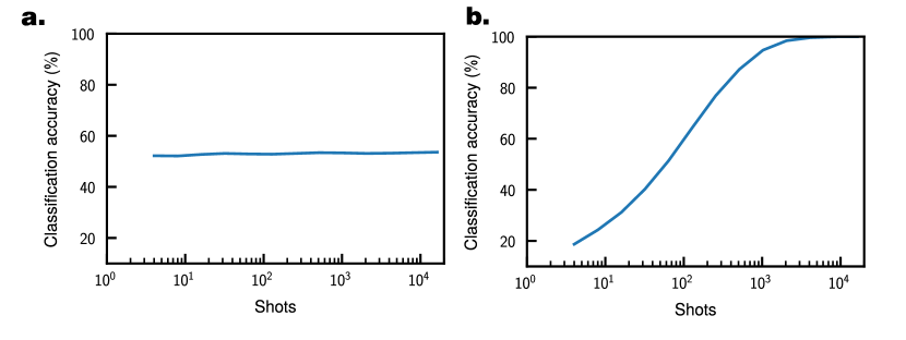
Figure M19: Performance of our reservoir protocol when the underlying system is governed by the Maxwell-Bloch equations of motion given by Eqs. 56,57,58, with the features used being third-order central moments between the outcome of four measurement pairs (cavity parity and qubit excitation). The subplots show performance for (a) spiral classification and (b) radio-frequency communication modulation protocol classification.

Finally, as for the CNOD operation, the way this was implemented in our experimental reservoir involved two opposite displacements at the same frequency, with a $\pi$-pulse on the qubit in between. Note, however, that in the mean field approximation, $\langle\sigma_{z}a\rangle=\langle\sigma_{z}\rangle\langle a\rangle$, and since our qubit was on the Bloch sphere equator during exposure to data and application of CNOD, this term goes to zero (and any deviation from the Bloch equator is due to noise and contains no information). Therefore, $\langle a\rangle$ depends on the drive term only, and CNOD has no effect on the cavity, as the cavity is displaced and then undisplaced by an equal amount. Since the only significant term affecting the qubit on the time-scale of the CNOD is the $|\langle a\rangle|^{2}$ term, which increases and decreases symmetrically about the $\pi$ pulse applied to the qubit, the effect of the cavity is cancelled out and the entire procedure is equivalent to only a $\pi$-pulse on the qubit. This is, therefore, the only part our CNOD that survived in the “classicalized” version of our reservoir control protocol.

Transferring our reservoir controls into the Maxwell-Bloch setting: investigating our protocol’s performance in a classical setting

As seen in Fig. M19(a), simulations of our reservoir using Maxwell-Bloch for classifying spiral, yielded classification accuracies that were no better than that of random guessing. The reason for this is that every point in the spiral has a point in the opposite class with identical magnitude but opposite phase in the quadrature space. However, the Maxwell-Bloch version of our reservoir is unable to differentiate two time-independent signals with identical magnitudes. As discussed in the previous section, our version of CNOD only affects the qubit with a $\pi$-pulse operation. Therefore, the only changes to the cavity are due to displacement caused by the data signal as a driving term, as seen from Eq. 56 since $\langle\sigma_{z}\rangle=0$ and so the qubit state does not influence our cavity during this stage. Consequently, when we measure cavity parity, this contains information about the magnitude of the signal but not its quadrature phase.

Depth, Reservoir size (R)	$w_{in}$	sparsity	$\rho$	$\gamma$	a
depth=4, $R\geq 64$	1.0	1.0	1.0	1.0	0
depth=4, $R=32$	1.0	0.2	1.0	1.0	0
depth=4, $R=16$	1.0	0.6	1.0	0.9	0.2
depth=4, $R=8$	1.0	0.6	0.9	0.8	0.5
depth=3, $R\geq 64$	1.0	0.2	1.0	1.0	0.5
depth=3, $R=32$	1.0	0.3	1.0	1.0	0
depth=3, $R=16$	1.0	0.45	1.0	1.0	0.2
depth=3, $R=8$	1.0	1.0	1.0	1.0	0.0
depth=2, $R\geq 64$	1.0	0.2	1.0	1.0	0.5
depth=2, $R=32$	1.0	0.3	1.0	1.0	0
depth=2, $R=16$	1.0	0.45	1.0	1.0	0.2
depth=2, $R=8$	1.0	1.0	1.0	1.0	0.0

Table S2: Hyper-parameters that were empirically found to give the best average spiral classification accuracy for each depth and size of reservoir.

The qubit, with the drives turned off, only has a dependence on the cavity in terms of $\langle\sigma_{z}\rangle|\langle a\rangle|^{2}$ as seen in Eq. 58. The qubit excitation probability, which we will obtain later after a $Y_{\frac{\pi}{2}}$ pulse is a nonlinear function of the integral of the cavity’s expected photon number over time. Therefore, information about the signal quadrature phase is absent from qubit measurements as well.

Importantly, this is a flaw that our particular reservoir protocol suffers from in the Maxwell-Bloch setting. For instance, having unconditional displacements, that differ for each run of the reservoir, could help turn quadrature phase information in the signal into information about the storage cavity’s displacement.

This limitation interestingly had a very minimal effect on the performance of the classicalized reservoir when it came to classifying radio-frequency communication modulations. This can be seen in Fig. M19(b), whose shot-limited accuracies were close to those of the quantum reservoir simulation accuracies of Fig. M15(b) with the same number of central moments. This is likely because differences between consecutive quadrature phases of incoming signals now introduce interactions that affect both qubit and cavity.

Another point noticed in our investigation with Maxwell-Bloch was that, while the performance hierarchy of third-order-cumulant-based features outperforming the sampling feature was maintained (see Fig. M13), the advantage was dramatically lower. The lack of variation is the reason why only third-order central moments are plotted in Fig. M19, as the performance curves would lie on top of each other. There are several reasons for this. Firstly, there are no longer higher-order correlations present due to the effects of entanglement between excitation measurements of the qubit and parity measurements of the cavity. Secondly, since this framework does not consider the effects of measurement back-action this removes correlation structures across measurement times that the quantum version takes advantage of. Nevertheless, due to some degree of correlation across measurements due to the signal itself, a weak advantage to considering higher-order central moments, and limitations of shot noise, did result in advantages in classification accuracy. This highlights the computational benefits our system reaps from considering signal correlations and central moments emerge from the information contained there, rather than a consequence of introducing the nonlinearity required to compute these values (since introducing the same correlation features for Maxwell-Bloch did not substantially change accuracy).

Appendix J Leaky Echo State Networks (LESN)

Background

Leaky echo state networks [JAEGER2007] are a generalization of echo state networks (ESN) [jaeger2001echo] that were found to outperform their parent design in prediction and classification of slow dynamic systems, noisy time series and time-warped dynamic patterns [LESNREVIEW2022]. Given a sequence of inputs $\{u_{n}\}_{n=1}^{N},u_{n}\in\mathbb{R}^{D}$, the state of the LESN reservoir after the $n^{\text{th}}$, $x_{n}$, is given by the following equation:

$$x_{n}=(1-a\gamma)x_{n-1}+\gamma f\left(W_{\text{in}}u_{n}+W_{\text{res}}x_{n-1}\right).$$ (62)

Here, $a,\gamma$ are fixed hyper-parameters in $[0,1]$, and $f$ is a nonlinear activation function. $W_{\text{in}}$ is the $D\times R$ “encoding” matrix whose elements are selected uniformly at random from the interval $[-w_{in},w_{in}]$, where $D$ is the dimension of the input, $R$ is the dimension of the reservoir, and $w_{in}$ is a fixed hyper-parameter. $W_{\text{res}}$ is the $R\times R$ “reservoir” matrix. This matrix is constructed by first generating a matrix $W_{R}$, which is a random matrix whose elements are chosen to be zero with probability $1-p_{s}$ and a number sampled uniformly from the interval $[-1,1]$ with probability $p_{s}$. The largest-magnitude singular value of this matrix, $\lambda_{\text{max}}(W_{R})$ is computed, and the reservoir matrix $W_{\text{res}}$ is defined as:

$$W_{\text{res}}=\frac{\rho}{\left|\lambda_{\text{max}}(W_{R})\right|}W_{R}$$ (63)

where $\rho$ is a fixed scaling hyper-parameter. Finally, the $n^{\text{th}}$ output of the reservoir, $y_{n}$, is given by

$$y_{n}=W_{\text{train}}x_{n},$$ (64)

where $W_{\text{train}}$ is a $R\times C$ trainable linear layer, where $C$ is the dimension of the desired output vector.

Digital reservoir comparison

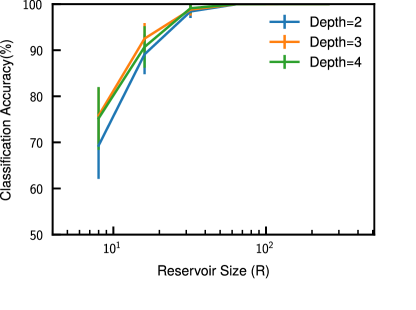
Figure M20: Mean spiral classification accuracies and their standard deviations over 100 randomly generated LESN’s. Hyper-parameters for all reservoir sizes $R$ (8,16,32,64,128,256) and depths (2,3,4) are specified in Tab. S2.

As a way of benchmarking the computational capacity of our physical reservoir, we compared it to the performance of a digital reservoir - an LESN - at varying widths and depths. We focused on the accuracy of classifying the spiral, since this is the most direct point of comparison, as the goal was to classify individual points of a signal rather, than multiple separate signals per-shot as with the time-dependent case. Here, for a depth of $N$, we sent in $N$ identical two-dimensional data points $(x,y)$ (so $D=2$) corresponding to the $I$ and $Q$ components of the signal that our experimental reservoir is meant to process, i.e. the spiral point coordinates. We used the rectified linear unit (ReLU) as our nonlinear activation function. Traditionally, sigmoid or tanh activation functions are used for LESN’s [JAEGER2007, LESNREVIEW2022, scardapane2017], but ReLU was found to work better for our application.

To investigate how “trivial” it was to generate a classifier with the same capacity as our experiment, we generated 100 such LESN’s at random, and found their average performance, and standard deviation. Hyper-parameters $a,\gamma,w_{\text{in}},\rho$, and sparsity ($p_{s}$) were tuned in sweeps to improve performance as much as possible for each width and depth, in order to give the digital reservoir a competitive chance. The reservoir’s computational capacity varies by the number of shots. Comparing Fig 2(b) to Fig M20, we found that, at around $10^{3}$ shots, our physical reservoir achieved a performance comparable to that of about that of a 32-dimensional LESN reservoir, as seen by the fact that both oscillate around 99$\%$ classification accuracy, within about one percent. In Fig M20, a 64-dimensional reservoir was found to be enough to classify the spiral data points with perfect accuracy and a fairly wide choice of parameters. Our reservoir, then, achieved at least the capacity of a, 64-dimensional LESN reservoir, past around $5*10^{3}$ shots. Given the roughly $2\times 16$ dimensions of Hilbert space used by our reservoir, this computational capacity is on the order of what would be expected for a large shot number.

References

- [1] (2022) Equivalence of quantum barren plateaus to cost concentration and narrow gorges. Quantum Science and Technology 7 (4), pp. 045015. External Links: Document, Link Cited by: Introduction.
- [2] (2019) Quantum supremacy using a programmable superconducting processor. Nature 574 (7779), pp. 505–510. External Links: Document, Link Cited by: Introduction.
- [3] (2023) Quantum advantage in microwave quantum radar. Nature Physics 19 (10), pp. 1418–1422. External Links: Document Cited by: Introduction, Discussion.
- [4] (2021) A quantum enhanced search for dark matter axions. Nature 590 (7845), pp. 238–242. External Links: Document Cited by: Introduction, Discussion.
- [5] (2017) Quantum machine learning. Nature 549 (7671), pp. 195–202. External Links: Document, Link Cited by: Introduction.
- [6] (2022) Quantum reservoir computing using arrays of rydberg atoms. PRX Quantum 3 (3), pp. 030325. Cited by: Introduction.
- [7] (2017) Roads towards fault-tolerant universal quantum computation. Nature 549 (7671), pp. 172–179. External Links: Document Cited by: Introduction.
- [8] (2022) Challenges and opportunities in quantum machine learning. Nature Computational Science 2 (9), pp. 567–576. External Links: Document Cited by: Introduction, Introduction, Discussion.
- [9] (2021) Variational quantum algorithms. Nature Reviews Physics 3 (9), pp. 625–644. External Links: Document, Link Cited by: Introduction.
- [10] (2020-08) Temporal information processing on noisy quantum computers. Phys. Rev. Appl. 14, pp. 024065. External Links: Document, Link Cited by: Introduction, Discussion.
- [11] (2022) Practical quantum advantage in quantum simulation. Nature 607 (7920), pp. 667–676. External Links: Document Cited by: Introduction.
- [12] (2012) Information processing capacity of dynamical systems. Scientific reports 2 (1), pp. 514. External Links: Document Cited by: Discussion.
- [13] (2023) Conditional not displacement: fast multi-oscillator control with a single qubit. External Links: 2301.09831 Cited by: Classification of time-independent signals.
- [14] (2017) Harnessing disordered-ensemble quantum dynamics for machine learning. Physical Review Applied 8 (2), pp. 024030. External Links: Document Cited by: Introduction.
- [15] (2021) Quantum reservoir computing: a reservoir approach toward quantum machine learning on near-term quantum devices. In Reservoir Computing: Theory, Physical Implementations, and Applications, K. Nakajima and I. Fischer (Eds.), pp. 423–450. External Links: ISBN 978-981-13-1687-6, Document, Link Cited by: Introduction.
- [16] (2021) Noise in digital and digital-analog quantum computation. External Links: 2107.12969 Cited by: Introduction.
- [17] (2021-09) Next generation reservoir computing. Nature Communications 12 (1). External Links: ISSN 2041-1723, Link, Document Cited by: Introduction.
- [18] (2019-04) Quantum reservoir processing. npj Quantum Information 5 (1). External Links: ISSN 2056-6387, Link, Document Cited by: Introduction.
- [19] (2022-08) Measurements as a roadblock to near-term practical quantum advantage in chemistry: resource analysis. Phys. Rev. Res. 4, pp. 033154. External Links: Document, Link Cited by: Introduction.
- [20] (2015-09) Cavity state manipulation using photon-number selective phase gates. Physical Review Letters 115 (13). External Links: ISSN 1079-7114, Link, Document Cited by: Experimental setup and protocols.
- [21] (2023-10) Tackling sampling noise in physical systems for machine learning applications: fundamental limits and eigentasks. Phys. Rev. X 13, pp. 041020. External Links: Document, Link Cited by: Experimental setup and protocols, Introduction, Discussion, Discussion.
- [22] (2023) Overcoming the coherence time barrier in quantum machine learning on temporal data. To appear on the arXiv. Cited by: Discussion.
- [23] Exploring communications technology – open university(Website) External Links: Link Cited by: Classification of radio-frequency (RF) communication modulation schemes.
- [24] (2012) Layered architecture for quantum computing. Physical Review X 2 (3), pp. 031007. External Links: Document Cited by: Introduction.
- [25] (2017) Hardware-efficient variational quantum eigensolver for small molecules and quantum magnets. nature 549 (7671), pp. 242–246. External Links: Document, Link Cited by: Introduction.
- [26] (2021) Physical reservoir computing using finitely-sampled quantum systems. External Links: 2110.13849 Cited by: Experimental setup and protocols, Introduction.
- [27] (2022) Quantum noise-induced reservoir computing. External Links: 2207.07924 Cited by: Introduction, Discussion.
- [28] (2010) Quantum computers. nature 464 (7285), pp. 45–53. External Links: Document Cited by: Introduction.
- [29] (2009) Reservoir computing approaches to recurrent neural network training. Computer science review 3 (3), pp. 127–149. External Links: Document, Link Cited by: Introduction.
- [30] (2020) Quantum neuromorphic computing. Applied physics letters 117 (15). External Links: Document, Link Cited by: Introduction.
- [31] (2021) Entanglement-induced barren plateaus. PRX Quantum 2 (4), pp. 040316. External Links: Document, Link Cited by: Introduction.
- [32] (2018) Barren plateaus in quantum neural network training landscapes. Nature communications 9 (1), pp. 4812. External Links: Document, Link Cited by: Introduction.
- [33] pyEPR: The energy-participation-ratio (EPR) open- source framework for quantum device design External Links: Document Cited by: Acknowledgements.
- [34] (2023) User trajectory prediction in mobile wireless networks using quantum reservoir computing. External Links: 2301.08796 Cited by: Introduction, Discussion.
- [35] (2017) Commercialize quantum technologies in five years. Nature 543 (7644), pp. 171–174. External Links: Document Cited by: Introduction.
- [36] (2020-02) Digital-analog quantum computation. Phys. Rev. A 101, pp. 022305. External Links: Document, Link Cited by: Introduction.
- [37] (2022-09) Hybrid quantum-classical reservoir computing of thermal convection flow. Physical Review Research 4 (3). External Links: ISSN 2643-1564, Link, Document Cited by: Introduction, Discussion.
- [38] (2018-08) Quantum computing in the nisq era and beyond. Quantum 2, pp. 79. External Links: ISSN 2521-327X, Link, Document Cited by: Introduction.
- [39] (2007) An overview of reservoir computing: theory, applications and implementations. In Proceedings of the 15th european symposium on artificial neural networks. p. 471-482 2007, pp. 471–482. Cited by: Introduction.
- [40] (2022) Is quantum advantage the right goal for quantum machine learning?. PRX Quantum 3 (3), pp. 030101. External Links: Document Cited by: Introduction.
- [41] (2022-01) Natural quantum reservoir computing for temporal information processing. Scientific Reports 12 (1). External Links: ISSN 2045-2322, Link, Document Cited by: Experimental setup and protocols, Introduction, Discussion.
- [42] (2022) The variational quantum eigensolver: a review of methods and best practices. Physics Reports 986, pp. 1–128. External Links: Document, Link Cited by: Introduction.
- [43] (2020-06) Efficient multiphoton sampling of molecular vibronic spectra on a superconducting bosonic processor. Phys. Rev. X 10, pp. 021060. External Links: Document, Link Cited by: Experimental setup and protocols.
- [44] (2021) Noise-induced barren plateaus in variational quantum algorithms. Nature communications 12 (1), pp. 6961. External Links: Document, Link Cited by: Introduction.
- [45] (2022) Quantum-enhanced radiometry via approximate quantum error correction. Nature Communications 13 (1), pp. 3214. External Links: Document Cited by: Introduction, Discussion.
- [46] (2021) Quantum microwave radiometry with a superconducting qubit. Physical Review Letters 126 (18), pp. 180501. External Links: Document Cited by: Introduction, Discussion.
- [47] (2019) The capacity of quantum neural networks. External Links: 1908.01364 Cited by: Experimental setup and protocols, Discussion.
- [48] (2023) Quantum reservoir computing with repeated measurements on superconducting devices. External Links: 2310.06706 Cited by: Experimental setup and protocols, Introduction, Classification of filtered noise, Discussion.
- [49] (2020-12) Quantum computational advantage using photons. Science 370 (6523), pp. 1460–1463. External Links: ISSN 1095-9203, Link, Document Cited by: Introduction.
- [50] (2020) Near-sensor and in-sensor computing. Nature Electronics 3 (11), pp. 664–671. External Links: Document Cited by: Discussion.

References

- [1] (2023) Conditional not displacement: fast multi-oscillator control with a single qubit. External Links: 2301.09831 Cited by: Appendix C, Figure M5, Figure M5, Appendix D, Appendix D.
- [2] (2021-09) Next generation reservoir computing. Nature Communications 12 (1). External Links: ISSN 2041-1723, Link, Document Cited by: Appendix E.
- [3] (2015-09) Cavity state manipulation using photon-number selective phase gates. Physical Review Letters 115 (13). External Links: ISSN 1079-7114, Link, Document Cited by: Appendix C.
- [4] (2012-08) QuTiP: an open-source python framework for the dynamics of open quantum systems. Computer Physics Communications 183 (8), pp. 1760–1772. External Links: ISSN 0010-4655, Link, Document Cited by: Appendix G.
- [5] (2022-01) QuantumCumulants.jl: A Julia framework for generalized mean-field equations in open quantum systems. Quantum 6, pp. 617. External Links: Document Cited by: Appendix I.
- [6] (2021) Noise-induced barren plateaus in variational quantum algorithms. Nature communications 12 (1), pp. 6961. External Links: Document, Link Cited by: Appendix C, Figure M6.
- [7] (2023) Quantum reservoir computing with repeated measurements on superconducting devices. External Links: 2310.06706 Cited by: Figure M16, Figure M16, Figure M16, Appendix G.