Large-scale Long-tailed Disease Diagnosis on Radiology Images

Abstract

In this study, we aim to investigate the problem of large-scale, large-vocabulary disease classification for radiologic images, which can be formulated as a multi-modal, multi-anatomy, multi-label, long-tailed classification. Our main contributions are three folds: (i), on dataset construction, we build up an academically accessible, large-scale diagnostic dataset that encompasses 5568 disorders linked with 930 unique ICD-10-CM codes, containing 39,026 cases (192,675 scans). (ii), on model design, we present a novel architecture that enables to process arbitrary number of input scans, from various imaging modalities, which is trained with knowledge enhancement to leverage the rich domain knowledge; (iii), on evaluation, we initialize a new benchmark for multi-modal multi-anatomy long-tailed diagnosis. Our method shows superior results on it. Additionally, our final model serves as a pre-trained model, and can be finetuned to benefit diagnosis on various external datasets.

1 Introduction

In the ever-evolving landscape of clinical medicine, the advent of radiology techniques, such as X-ray, CT, MRI, and ultrasound, has truly revolutionized the medical field, offering a non-invasive yet deeply revealing perspective of the human body for disease diagnosis and management. These imaging techniques are now at the cusp of a new era with the integration of artificial intelligence (AI).

Recent literature highlights the significant potential of developing diagnostic models in the medical field, the developments can be generally cast into two categories: one is a specialist, which has already shown success in identifying and managing a wide array of diseases [15, 78, 86]. However, a notable limitation of these models is their specialization, as they often focus on a narrow range of disease categories, targeting limited anatomical regions, based on specific imaging modalities. This specialization restricts their ability to fully address the diverse and complex cases encountered in real-world clinical settings.

While on the other extreme, there is an emerging trend towards developing Generalist Medical Artificial Intelligence (GMAI) models [56, 81, 85]. Taking inspiration from the breakthroughs in natural language processing and computer vision, these models aim to amalgamate data from diverse sources, including various imaging methods, patient histories, and current medical research, to offer more comprehensive diagnostic and treatment solutions. Nonetheless, the development of GMAI models faces formidable challenges, such as the need for substantial computational power, meticulously curated multimodal datasets covering an extensive range of medical conditions and patient demographics, and advanced models equipped to tackle unique medical intricacies, like extremely unbalanced data distribution and the need for domain-specific expertise.

In this paper, we consider the problem of large-scale, large-vocabulary disease classification for radiologic images, marking a transition phase between specialist and generalist models. Specifically, compared to existing specialists, we aim to initiate the research for developing a computational model that can handle multi-modal, multi-anatomy, and multi-label disease diagnosis, in the face of extremely unbalanced distribution, embracing a wider scope of diagnoses across various anatomical regions and imaging modalities. In contrast to generalist models, our investigation offers a more feasible and targeted playground for exploring sophisticated algorithms in academic labs, offering opportunities for detailed error analysis, which is often impractical in the development of large-scale generalist models due to prohibitive computational costs. Overall, we make contributions from three aspects, namely, a large-scale open dataset and its construction pipeline, preliminary model architecture exploration, and an evaluation benchmark.

On dataset construction, we build up an academically accessible, large-scale diagnostic dataset derived from Radiopaedia [5]. Each sample is associated to the International Classification of Diseases, i.e., ICD-10-CM [1], indicating the diagnostic category, for example, ‘S86’ refers to ‘Injury of muscle, fascia and tendon at lower leg level’. The dataset naturally displays an unbalanced distribution, varying from 1 to 964 cases in each disease category. Additionally, each case within the dataset involves multiple multi-modal scans, with the number of modalities ranging from 1 to 5, the number of images per case spanning between 1 and 30. As a result, we construct a long-tailed, multi-scan medical disease classification dataset, as shown in Figure 1, with 39,026 cases (192,675 scans) across 7 human anatomy regions and 9 diverse modalities covering 930 ICD-10-CM codes, 5568 disorders, termed as Radiopaedia3D Diagnosis Dataset (RP3D-DiagDS). We will release all the data, complete with corresponding disorders, ICD-10-CM codes, and detailed definitions.

On architecture design, we demonstrate a new model that supports both 2D and 3D input from various modalities, together with a transformer-based fusion module for comprehensive diagnosis. Specifically, for visual encoding, we explore two variants of backbones, namely, ResNet-based, and ViT-based to perform 2D or 3D unified encoding. Then we fuse the multi-scan information with a transformer-based fusion module, treating each image embedding as an input token. At training time, we adopt knowledge-enhanced training strategy [79, 84], specifically, we leverage the rich domain knowledge to pre-train a knowledge encoder with natural language and use it to guide the visual representation learning for disease diagnosis.

On evaluation, we carry out a series of ablation studies on the effectiveness of different training configurations, for example, visual backbones (ViT or ResNet), augmentation implementation, and depth of 3D input volumes. Then, we evaluate the model on our proposed benchmark of multi-modal multi-scan long-tailed multi-label diagnosis and demonstrate the superiority of our proposed methods on it. Furthermore, our trained model showed strong transferring abilities. By fine-tuning, it can benefit numerous external datasets, regardless of their image dimensions, imaging modalities, and shooting anatomies.

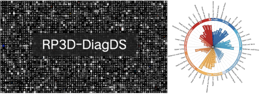
Figure 1: Overview of RP3D-DiagDS. There are 39,026 cases (192,675 scans) across 7 human anatomy regions and 9 diverse modalities covering 930 ICD-10-CM codes.

2 Related Work

2.1 Disease Classification Datasets

Open-source datasets play a crucial role in the development of AI for medical image analysis. Unlike natural images, the curation of medical image datasets presents unique challenges due to factors, such as privacy concerns, requirement of specialized domain knowledge for annotation, etc. In the literature, there has been a number of open-source datasets for disease diagnosis. Notably, large-scale datasets such as NIH ChestX-ray [76], MIMIC-CXR [38], and CheXpert [34] stand out for their comprehensive collection of annotated X-ray images, facilitating extensive research and advancements in automated disease classification. However, it’s important to note three key limitations. First, these open-source diagnosis datasets mainly consist of consist of chest X-rays [63, 12, 76, 34, 50, 66, 31, 36, 71, 25, 59, 22, 38, 19], thus are 2D images. There are only a few 3D datasets available, with a limited number of volumes [54, 3, 2, 4, 39, 43, 51, 33, 58, 66, 10, 7, 9]. Second, a significant portion of these large-scale datasets focuses solely on binary classification of specific diseases [71, 25, 31, 36]. Third, existing large-scale datasets containing a broad range of disease categories in different granularities [12, 82, 53], for example, in PadChest [12], disorders exist at different levels, including infiltrates, interstitial patterns, and reticular interstitial patterns. Such variation in granularity poses a great challenge for representation learning. In summary, these datasets fall short of meeting real-world clinical needs, which often involve complex, multimodal, and multi-image data from single patient. Therefore, constructing a dataset that mirrors the intricacies of actual clinical scenarios is necessary.

2.2 Specialist Diagnosis Models

The prevailing paradigm in earlier diagnostic models is a specialized model trained on a limited range of disease categories. These models focus on specific imaging modalities and are targeted towards particular anatomical regions. Specifically, ConvNets are widely used in medical image classification due to its outstanding performance, for example, [21, 69, 73, 29, 19, 46, 13, 74] have demonstrated excellent results on identifying a wide range of diseases. Recently, Vision Transformer (ViT) has garnered immense interest in the medical imaging community, numerous innovative approaches  [20, 80, 27, 70, 52, 87, 83, 65, 84, 67, 79, 48, 72, 26, 55] have emerged, leveraging ViTs as a foundation for further advancements in this field.

2.3 Generalist Medical Foundation Models

The other stream of work is generalist medical foundation models  [75, 81, 56, 85]. These models represent a paradigm shift in medical AI, aiming to create versatile, comprehensive AI systems capable of handling a wide range of tasks across different medical modalities, by leveraging large-scale, diverse medical data. MedPaLM M [75] reaches performance competitive with or exceeding the state-of-the-art (SOTA) on various medical benchmarks, demonstrating the potential of the generalist foundation model in disease diagnosis and beyond. RadFM [81] is the first medical foundation model capable of processing 3D multi-image inputs, demonstrating the versatility and adaptability of generalist models in processing complex imaging data. However, the development of GMAI models requires substantial computational power, which is often impractical for exploring sophisticated algorithms in academic labs.

2.4 Long-tailed Classification Strategy

Medical image diagnosis inherently faces long-tail challenges, as the prevalence of common diseases is usually substantially higher than that of rare diseases. A straightforward solution to the imbalance problem is to perform re-sampling during training [24, 28, 42, 49], e.g., over-sampling on tailed classes or under-sampling on head classes. However, this approach often triggers over-fitting in tail classes, resulting insufficient training for the head classes. Loss re-weighting is another widely used solution to tackle the long-tailed distribution problem [47, 68]. Focal loss [45, 47] refines cross-entropy by assigning lower weights to easily learnable data, thereby prioritizing challenging or misclassifiable instances. These approaches have primarily been explored on relatively small datasets with a limited number of categories. In this paper, our objective is to initiate the problem for large-scale, long-tailed, multi-scan medical disease classification.

3 Dataset Construction

In this section, we present the details of our dataset, RP3D-DiagDS, that follows a similar procedure as RP3D [81]. Specifically, cases in our dataset are sourced from the Radiopaedia website [5] – a growing peer-reviewed educational radiology resource website, that allows the clinicians to upload 3D volumes to better reflect real clinical scenarios. Additionally, all privacy issues have already been resolved by the clinicians at uploading time. It is worth noting that, unlike RP3D [81] that contains paired free-form text description and radiology scans for visual-language representation learning, here, we focus on multi-modal, multi-anatomy, and multi-label disease diagnosis (classification) under extremely unbalanced distribution.

Overall, the proposed dataset contains 39,026 cases, of 192,675 images from 9 diverse imaging modalities and 7 human anatomy regions, note that, each case may contain images of multiple scans. The data covers 5,568 different disorders, that have been manually mapped into 930 ICD-10-CM [1] codes.

3.1 Data Collection

Here, we describe the procedure of our data curation process, shown in Figure 2. Specifically, we collect three main components from each case on Radiopaedia webpage, namely, ‘Patient data’, ‘Radiology images’, and ‘Articles’  (example webpage shown in Figure 2 (a)). ‘Patient data’ includes brief information of this patient, for example, age, gender, etc. ‘Radiology images’ denote a series of radiology examination scans. Figure 5 (a) provides a statistical analysis on the number of images within one single case. ’Articles’ contains links to related articles named with corresponding disorders, which are treated as diagnosis labels and have been meticulously peer-reviewed by experts in Radiopaedia Editorial Board.

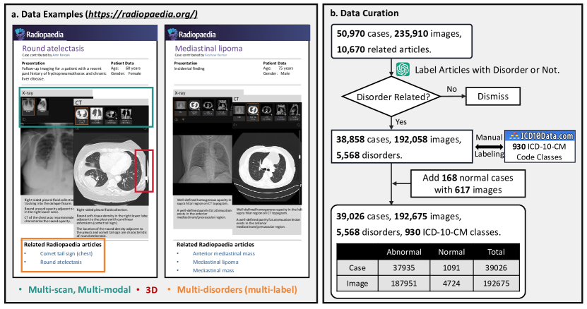
Figure 2: The data collection pipeline. In (a) we show two original cases. Our dataset presents a multi-scan multi-modal multi-label long-tailed diagnosis task with 2D and 3D scan involed. In (b) we show the general data curation progress. We totally collect 39026 cases with 192675 images labeled by 5568 disorder classes and 930 ICD-10-CM classes. In addition to the intermediate case number, we also show the intermediate image number together with the final normal and abnormal case number in (b).

To start with, we can collect 50,970 cases linked with 10,670 articles from Radiopaedia website. However, naively adopting the article titles as disorders may lead to ambiguities from two aspects: (i) not all articles are related to disorders, (ii) article titles can be written with different granularity, for example, “pneumonia” and “bacterial pneumonia” can be referred to as different disorders, though they should ideally be arranged in a hierarchical structure, (iii) normal cases from Radiopaedia are not balanced in modalities and anatomies. Next, we discuss 3-stage procedure to alleviate the above-mentioned challenges.

Article Filtering. We leverage the GPT-4 [64] to automatically filter the article list, leaving those refer to disorders. Specifically, taking inspiration from the self-consistency prompts [77], we design two different query prompts with similar meanings, as shown in Figure 3 (a). An article name is labeled as disorder if GPT-4 gives consistent positive results from both prompts, while for those GPT-4 gives inconsistent results, we do manually check them. To measure the quality for filtering, we randomly sample a portion of data for manual checking to control its quality. The confusion metrics are shown in Figure 3 (c). The $100\%$ precision score indicates our auto-filtering strategy, can strictly ensure the left ones to be disorders. Eventually, 5342 articles can pass the first auto-criterion and 226 pass the second manually checking, resulting in 5,568 disorder classes, as shown in Figure 2 (b). Cases not linked to any articles are excluded, ultimately yielding 38,858 cases.

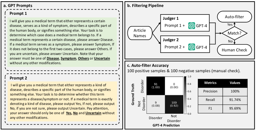
Figure 3: The article filtering pipeline. In (a), we show the two GPT prompts and (b) is the whole pipeline where we leverage the two prompts to query GPT-4 twice and only the consistent results will be used for auto-filtering, otherwise, we will check it manually. (c) shows the accuracy of the auto-filtering cases. Note that, all the 200 article samples evaluated in (c) have a consistent prediction under the two GPT-4 prompts.

Mapping disorders to ICD-10-CM. Upon getting disorder classes, they may fall into varying hierarchical granularity levels, here, we hope to map them to internationally recognized standards. For this purpose, we utilize the International Classification of Diseases, Tenth Revision, Clinical Modification (ICD-10-CM) codes, which is a customized version of the ICD-10 used for coding diagnoses in the U.S. healthcare system. The ICD was originally designed as a health care classification system, providing a system of diagnostic codes for classifying diseases, including nuanced classifications of a wide variety of signs, symptoms, abnormal findings, complaints, social circumstances, and external causes of injury or disease. Specifically, we hire ten medical PhD students to manually map the article titles into ICD-10-CM codes. After cross-checking by a ten-year clinician, we have mapped the 5,568 disorders into the corresponding ICD-10-CM codes. We unify various disorders into the first hierarchical level of ICD-10-CM code tree, resulting in 930 ICD-10-CM classes. For example, both “J12.0 Adenoviral pneumonia” and “J12 Viral pneumonia” are mapped to the code “J12 Viral pneumonia, not elsewhere classified”, dismissing the ambiguities caused by diagnosis granularity. Note that, we will provide the ICD-10-CM codes along with the original 5,568 classes, each accompanied by its corresponding definition, thus, the dataset can be employed for training diagnosis or visual-language models.

Adding Normal Cases. Despite there are normal cases on Radiopaedia, covering most of anatomies and modalities, we additionally collect more normal cases from MISTR, with images available for research under a CC-BY-NC-SA 4.0 license. The expanded normal cases include 168 cases. The distribution of modalities and anatomical regions will be shown in the data statistics section later.

Finally, we get 39,026 cases containing 192,675 images labeled by 5,568 disorder classes and 930 ICD-10-CM classes and will continually maintain the dataset, growing the case number.

3.2 Dataset Statistics

In this section, we provide detailed analysis on our proposed dataset, from three aspects, namely, modality coverage, anatomy coverage, and disease coverage.

Table 1: Comparison between RP3D-DiagDS and existing disease diagnosis datasets. #Image refers to the number of images in the dataset. #Disorders represents the number of categories of labeled disorders. 2D/3D indicates the dimension of images in the dataset, and the case-level column indicates whether the dataset contains multiple images per patient. Our dataset demonstrates significant increase in both size and diversity.

Dataset	Anatomy	Modality	#Image	#Disorders	2D	3D	Case-level
Brain-Tumor [3]	Head and Neck	MRI	7k	4	✓	✗	✗
CE-MRI  [17]	Head and Neck	MRI	3k	3	✓	✗	✗
Brain-Tumor-17  [4]	Head and Neck	MRI	4.4k	17	✓	✗	✗
OASIS[39, 43, 51]	Head and Neck	MRI	3.2k	2	✓	✗	✗
ICH2020 [33]	Head and Neck	CT	82	5	✗	✓	✗
COVID19-CT-DB [58]	Chest	CT	1k	9	✓	✗	✗
Covid-CXR2 [66]	Chest	X-ray	19k	3	✓	✗	✗
POCUS [10]	Chest	Ultrasound	1.1k	3	✓	✗	✗
MIA-COV19 [40]	Chest	CT	5.3k	2	✗	✓	✗
LIDC-IDRI [7]	Chest	CT	1.0k	3	✓	✗	✗
NIH Chestxray [76]	Chest	X-ray	100k	14	✓	✗	✗
PadChest [12]	Chest	X-ray	160k	193	✓	✗	✗
CheXpert [34]	Chest	X-ray	224k	14	✓	✗	✗
RSNA [71]	Chest	X-ray	30k	2	✓	✗	✗
SIIM-ACR [25]	Chest	X-ray	15k	2	✓	✗	✗
MIMIC-CXR [38]	Chest	X-ray	371k	14	✓	✗	✗
VinDr-CXR [59]	Chest	X-ray	18k	28	✓	✗	✗
VinDr-PCXR [63]	Chest	X-ray	9k	51	✓	✗	✗
VinDr-Mammo [61]	Breast	Mammography	20k	10	✓	✗	✗
DDSM [32, 44]	Breast	Mammography	55k	5	✓	✗	✗
CMMD2022 [14]	Breast	Mammography	5.2k	2	✓	✗	✗
BUSI [6]	Breast	Ultrasound	780	3	✓	✗	✗
VinDr-SpineXr [62]	Spine	X-ray	10k	13	✓	✗	✗
MRNet [9]	Knee	MRI	1370	3	✓	✗	✗
DeepLesion [82]	Whole body	Radiology	32k	22	✓	✗	✗
RadImageNet [53]	Whole body	CT, MRI, Ultrasound	1.35M	165	✓	✗	✗
RP3D-DiagDS (ours)	Whole body	Radiology	192k	5568 (ICD-10-CM:930)*	✓	✓	✓

• We map disorders to ICD-10-CM for standardization.

Analysis on Modality Coverage. RP3D-DiagDS comprises images from 9 modalities, namely, computed tomography (CT), magnetic resonance imaging (MRI), X-ray, Ultrasound, Fluoroscopy, Nuclear medicine, Mammography, DSA (angiography), and Barium Enema. Each case may include images from multiple modalities, to ensure precise and comprehensive diagnosis of disorders. Overall, approximately 19.4% of the cases comprise images from two modalities, while around 2.9% involve images from three to five modalities. The remaining cases are associated with image scans from a single modality. The distribution of modalities among all abnormal samples is illustrated in Figure 4 (a). The modalities of normal cases follow similar distributions with the abnormal cases, as shown in Figure 4 (b).

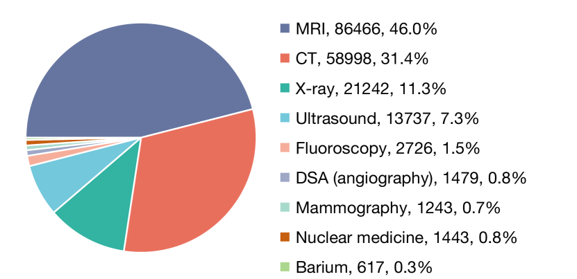
(a) Abnormal Cases Distribution in Modality

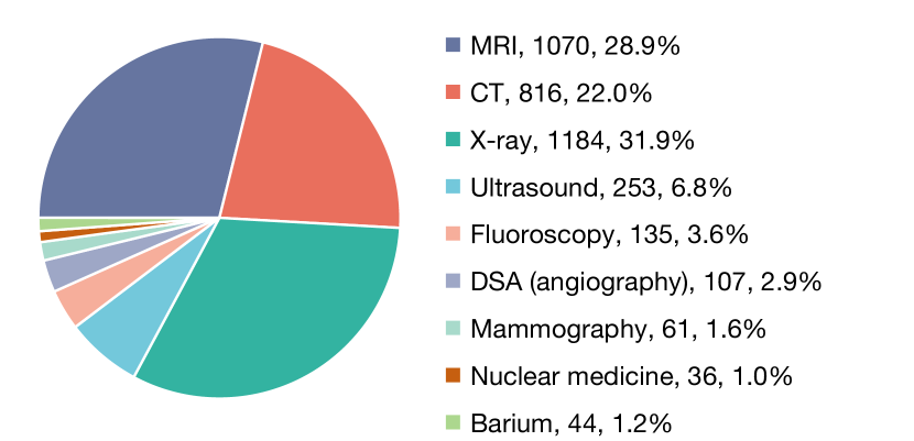
(b) Normal Cases Distribution in Modality

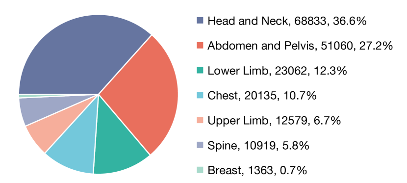
(c) Abnormal Cases Distribution in Anatomy

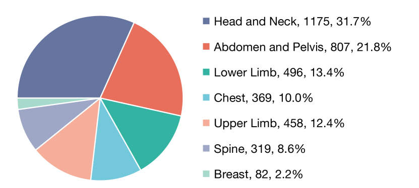
(d) Normal Cases Distribution in Anatomy

Figure 4: The distribution of imaging modalities of abnormal (a) and normal (b) cases in RP3D-DiagDS and anatomies of abnormal (c) and normal (d) cases in RP3D-DiagDS. Each label is annotated with the class name, number of cases, and the corresponding proportion.

Analysis on Anatomy Coverage. RP3D-DiagDS comprises images from various anatomical regions, including the head and neck, spine, chest, breast, abdomen and pelvis, upper limb, and lower limb, providing comprehensive coverage of the entire human body. The statistics are shown in Figure 4 (c) and 4 (d).

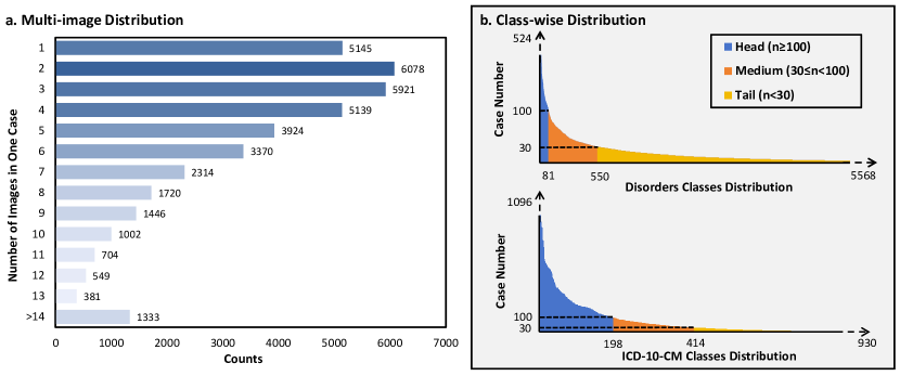
Figure 5: Distribution Analysis. In (a), we show the distribution for the number of images in one case. Each case may include multiple images from patient history scans, different modalities, different angles or conditions. In (b), we demonstrate the long-tailed distributions for disorder and ICD-10-CM classes. We also categorize these classes into three categories: “head class”, “body class” and “tail class” based on the number of cases. Notably, to better show the main part of the case distributions in (b), we clip the axes, indicated by the dotted axes lines.

Analysis on Disease Coverage. For both disorder and disease classification, each case can correspond to multiple disorders, resulting in RP3D-DiagDS a multi-label classification dataset. As shown in Figure 5 (b), the distributions exhibit extremely long-tailed pattern, rendering such 2D & 3D image classification problem as a long-tailed multi-label classification task. We define the ‘head class’ category with case counts greater than 100, the ‘body class’ category with case counts between 30 and 100, and the ‘tail class’ category with case counts less than 30.

4 Method

In this section, we aim to initiate a preliminary investigation on computational architectures for large-scale, long-tailed disease diagnosis on radiology, specifically, we start by defining the problem of case-level multi-label classification in Sec. 4.1, then we elaborate the architecture in Sec. 4.2, and knowledge-enhanced training strategy in Sec. 4.3.

4.1 Problem Formulation

We consider one case with its disease labels, represented as $\mathcal{X}=\{x_{1},\dots,x_{S},y_{1},\dots,y_{c}\}$, where $x_{i}$ denotes a specific scan (2D or 3D) under a certain radiologic examination, for example, MRI, CT or X-ray within $\mathcal{X}$, $S$ denotes the scan number for the case and $c$ represents the total diagnostic labels. Note that, there may be multiple scans from the same or different modalities for each patient.

To illustrate this concept, consider a case where a patient undergoes a physical examination, including a chest CT and a chest X-ray as shown in Figure 6. In this instance, $S=2$ reflects the two scans involved in this case. If the patient is diagnosed with nodule and pneumothorax, the labels for these diseases are set to 1, reflecting their presence in the patient’s diagnosis.

Our goal is to train a model that can solve the above multi-class, multi-scan diagnosis problem:

$$\mathcal{Y}=\Phi(\mathcal{X})=\Phi_{\text{cls}}(\Phi_{\text{fuse}}(\Phi_{\text{visual}}(x_{1}),\Phi_{\text{visual}}(x_{2}),\cdots,\Phi_{\text{visual}}(x_{S})))\in\mathcal{R}^{c},$$ (1)

the model is composed of a visual encoder $\Phi_{\text{visual}}$, a fusion module $\Phi_{\text{fuse}}$ and a classifier $\Phi_{\text{cls}}$.

4.2 Architecture

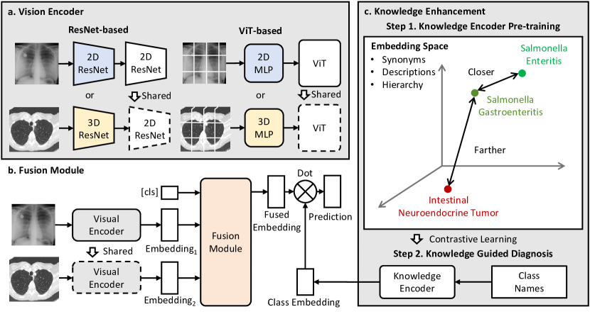
Figure 6: The architecture of our proposed visual encoder and fusion module, together with the knowledge enhancement strategy. (a) shows the details of the vision encoder. We design two variants to fit in the two main visual backbones, i.e., ResNet and ViT. (b) shows the transformer-based fusion module, enabling case-level information fusion. (c) shows the knowledge enhancement strategy. We first pre-train a text encoder with extra medical knowledge with contrastive learning, i.e., synonyms, descriptions and hierarchy, termed as knowledge encoder and then we view the text embedding as a natural classifier to guide the diagnosis classification.

Our proposed architecture consists of two key components: (i) a visual encoder that processes 2D or 3D input scan; (ii) a transformer-based fusion module, merging all information to perform case-level diagnosis.

4.2.1 Visual Encoder

We consider two popular variants of the visual encoder, namely, ResNet [30] and ViT [23], as shown in Figure 6 (a). The visual encoding progress can generally be formulated as:

$$v_{i}=\Phi_{\text{visual}}(x_{i})\in\mathcal{R}^{d}.$$ (2)

where $x_{i}\in\mathcal{R}^{C\times H\times W\times(D)}$ denotes the input scan, $C,H,W$ refer to the image channel, height and width of the input scan respectively. $D$ is optional, and only available for 3D input scans. The main challenge for architecture design comes from the requirement to process scans in both 2D and 3D formats. Here, we train separate normalisation modules to convert the 2D or 3D inputs into feature maps of same resolution, and further passed into shared encoding module.

ResNet. For 3D scans, they are first fed into 3D ResNet, followed by average pooling on depth to aggregate the information of the extra dimension; while for 2D scans, they are fed to the 2D ResNet to perform the same down-sampling ratio on height and width as for 3D. After normalization, both 2D and 3D scans are transformed into feature maps with same resolution, $f_{i}\in\mathcal{R}^{d_{\text{res}}\times h\times w}$, where $d_{\text{res}}$ is the intermediate feature dimension and $h,w$ denote the normalized size. Then, the feature maps are passed into a shared ResNet to get the final visual embedding.

ViT. For 3D scans, we convert the input volume into a series of non-overlapped 3D cubes, and pass them into MLP projection layers, to get vector embeddings; while for 2D scans, the input scan is broken into 2D patches, and projected into vector embeddings with another set of MLP layers. As ViT enables to handle sequences of variable tokens, we can now pass the resulting vectors into a shared ViT to get the final visual embedding. For position embedding, we adopt two sets of learnable position embeddings, one for 2D input, the other for 3D, further indicating the network about the input dimenstion.

4.2.2 Fusion Module

For case-level diagnosis, we propose to aggregate information from multiple scans with a trainable module. As shown in Figure 6 (b), we adopt transformer encoders, specifically, we first initialize a set of learnable modality embeddings, denoted as $\{p_{1},\dots,p_{M}\}$, where $M$ denotes the total number of possible imaging modalities. Given certain visual embedding ($v_{i}$) from modality $j$, we first add the corresponding modality embedding ($p_{j}$) to it, indicating which radiologic modality it is from. Then we feed all visual embeddings from one case into the fusion module, and output the fused visual embedding $v_{\text{fuse}}\in\mathcal{R}^{d}$, from the “[cls]” token, similar to paper [23], denoted as:

$$v_{\text{fuse}}=\Phi_{\text{fuse}}(\Phi_{\text{visual}}(x_{1}),\Phi_{\text{visual}}(x_{2}),\cdots,\Phi_{\text{visual}}(x_{S}))\in\mathcal{R}^{d}.$$ (3)

Till here, we have computed the case-level visual embedding, which can be passed into classifier for disease diagnosis. Here, we adopt a knowledge-enhanced training strategy [79, 84], that has shown to be superior in long-tailed recognition problem, as detailed in the following section.

4.3 Knowledge-enhanced Training

With knowledge enhancement, we hope to leverage the rich domain knowledge in medicine to enhance the long-tailed classification. Our key insight is that the long-tailed diseases may fundamentally have some shared symptoms or radiologic pathologies with the head classes, which could be encoded in text format.

In detail, we first pre-train a text encoder with medical knowledge, termed as knowledge encoder, where names of similar disorder or diseases are projected to similar embeddings, for example, ‘lung disease’ is closer to ‘pneumonia’ in the embedding space than ‘brain disease’. Then we freeze the text embeddings, and use them to guide the training of vision encoder, as shown in Figure 6 (c).

Knowledge Encoder Pre-training. We leverage several extra knowledge bases to pre-train a knowledge encoder, including Radiopaedia, ICD10-CM, and UMLS. Specifically, for each disorder term, we collect its definitions, radiologic features from Radiopaedia articles, synonyms, clinical information, and hierarchy structure from ICD10-CM, as well as definitions from UMLS. We aim to train the text encoder with the following considerations:

• Synonyms. If two terms are identified as similar synonyms, we expect them to be close in text embedding space, like ‘Salmonella enteritis’ and ‘Salmonella gastroenteritis’.

• Hierarchy. In the context of hierarchical relationships, we expect that if a disease is a fine-grained classification of another disease, its embeddings should be closer than those of unrelated diseases. For example, ‘J93, Pneumothorax and air leak’ should exhibit closer embeddings with ‘J93.0, Spontaneous tension pneumothorax’ than with ‘J96.0, Acute respiratory failure’.

• Descriptions. For terms associated with descriptions, radiologic features or clinical information, we expect their embeddings to be close in the text embedding space. For example, ‘Intestinal Neuroendocrine Tumor’ and ‘A well-differentiated, low or intermediate grade tumor with neuroendocrine differentiation that arises from the small or large intestine’.

We start from an off-the-shelf text encoder, namely, MedCPT-Query-Encoder [37], and adopt contrastive learning for further finetuning. Given a target medical terminology name encoded by the text encoder, denoted as $f_{\text{tar}}$, its corresponding medical texts, i.e., synonyms, containing terminologies or related descriptions are treated as positive cases. Similarly, we encode them with the text encoder, denoted as $f^{+}$, and other non-related text embedding is treated as negative cases $f^{-}$. Note that, we keep positive and negative cases consistent in format, e.g., when the positive case is related to description sentence, the negative cases are always some non-related description sentences instead of the short name words. The final objective can be formulated as:

$$\mathcal{L}_{\text{knowledge}}=-\log\frac{e^{f_{\text{tar}}^{T}\cdot f^{+}/\tau}}{\sum_{n=1}^{N}e^{f_{\text{tar}}^{T}\cdot f^{-}_{n}/\tau}},$$ (4)

where $\tau$ refers to the temperature, and $N$ denotes total sampled negative cases. By optimizing the contrastive loss we can further finetune the text encoder, resulting in a knowledge encoder, termed as $\Phi_{k}$

Knowledge-guided Classification. After training the knowledge encoder, we use it to encode the disorder/disease names into text embeddings, for example, denoting the names as $\{T_{1},T_{2},\dots,T_{c}\}$, where $T_{j}$ is a disorder/disease name like “pneumonia” or “lung tumor”. We embed these free texts with the knowledge encoder as:

$$t_{j}=\Phi_{k}(T_{j})\in\mathcal{R}^{d},$$ (5)

where $t_{j}$ denotes the text embedding. The resulting text embeddings are used for case-level diagnosis:

$$p=v_{\text{fuse}}\cdot t\in\mathcal{R}^{c},$$ (6)

where $p$ is the final result. We use classical binary cross entropy (BCE) loss as the final training objective, denoted as:

$$\mathcal{L}=-\sum_{i=1}^{c}\mathcal{Y}_{i}\cdot\log(p_{i})+(1-\mathcal{Y}_{i})\cdot\log(1-p_{i}).$$ (7)

5 Experiments

In this section, we will introduce our evaluation settings. Specifically, we first establish a benchmark for case-level multi-modal, multi-scan, long-tailed disorder/disease diagnosis. Second, we treat RP3D-DiagDS as a large-scale dataset for pre-training, and evaluate its transferring ability to various existing datasets.

5.1 Long-tailed Classification on RP3D-DiagDS

With the proposed dataset, we consider the problem as a multi-label classification task under a long-tailed distribution. In this section, we provide an overview of the training and evaluation protocols employed in our study. We first introduce the dataset split, followed by details of evaluation metrics for assessment.

5.1.1 Dataset Split

We randomly split our dataset into training (train and validation) and test sets in a (7:1):2 ratio. We treat the class with $[100:]$ positive cases as head classes, $[30,100)$ cases as medium classes, and $[:30)$ cases as tail classes. Consequently, from a total of 38,858 cases, the training set comprises 27,201 cases, and the test set includes 7,772 cases. Following on the dataset construction procedure, we perform classification task on two class sets at different granularities: (i) 5568 disorders + normal; (ii) 930 ICD-10-CM codes + normal. On different sets, we will have different head/medium/tail class set following our definition. Note that, the normal class is always treated as one of the head classes. Next, we will only talk about the abnormal classes.

Disorders. At the disorder level, there are 85 head classes, 470 medium classes, and 5014 tail classes. Notably, as the case number of some tailed classes is extremely small, some classes may only appear in training or test sets, but not both. This issue only happens to the tail classes. It is important to note that our knowledge encoder enables to get embedding for unseen diseases, ensuring that evaluation is not affected by such challenge. As a result, there are 5,305/3,399 classes in our training and testing split, respectively.

ICD-10-CM. At ICD-10-CM level, disorders with similar meanings have been mapped to same codes, for example, ‘tuberculosis’, ‘primary pulmonary tuberculosis’ all correspond to ‘A15 respiratory tuberculosis’. This merge operation results in more cases in one class, consequently more head classes. Specifically, we have 165 head classes, 230 medium classes, and 536 tail classes. Similarly, some tail classes may only be in training or testing split, resulting in 902/759 classes for our final training and testing splits, respectively.

It is important to point that while we ensure the inclusion of head and medium classes in both the training and test sets, some tail classes are inevitably exclusive from certain divisions, which is treated as our future work to collect more samples of such disorders. We report the results separately for head/medium/tail classes, while focusing primarily on the head classes.

5.1.2 Evaluation Metrics

In this section, we describe the evaluation metrics in detail. Note that, the following metrics can all be calculated per class. For multi-class cases, we all use macro-average on classes to report the scores by default. For example, “AUC” for multi-class classification denotes the “Macro-averaged AUC on classes”.

AUC. Area Under Curve [11] denotes the area under ROC (receiver operating characteristic) curve. This has been widely used in medical diagnosis, due to its clinical meanings and robustness in unbalanced distribution.

AP. Average Precision (AP) is calculated as the weighted mean of precisions at each threshold. Specifically, for each class, we rank all samples according to the prediction score, then shift the threshold to a series of precision-recall points and draw the precision-recall (PR) curve, AP equals the area under the curve. This score measures whether the unhealthy samples are ranked higher than healthy ones. We report Mean Average Precision (mAP), which is the average of AP of each class.

F1 and MCC. F1 score is the harmonic mean of the precision and recall. It is widely used in diagnosis tasks. MCC [18] denotes the Matthews Correlation Coefficient metric. It ranges from $-1$ to $1$ and can be calculated as follow:

$$\text{MCC}=\frac{\text{TN}\times\text{TP}-\text{FN}\times\text{FP}}{\sqrt{(\text{TP}+\text{FP})(\text{TP}+\text{FN})(\text{TN}+\text{FP})(\text{TN}+\text{FN})}}$$

Both metrics need a specific threshold to compute, and we choose one by maximizing F1 on the validation set following former papers [59, 79, 80, 84].

Recall@FPR. We also report the recall scores at different false positive rate (FPR), i.e., sample points from class-wise ROC curves. Specifically, We report the Recall@0.01, Recall@0.05, Recall@0.1 score, denoting the recall scores at 0.01, 0.05, 0.1 FPR respectively.

5.2 Transfer Learning to External Datasets

In addition to evaluating on our own benchmark, we also consider transferring our final model to other external datasets, demonstrating its transferring abilities on image distribution shift and label space change. In the following sections, we start by introducing the used external datasets, that cover various medical imaging modalities and anatomies. Then we detail the fine-tuning settings.

5.2.1 External Datasets

We choose external evaluation dataset with the following principles:

• Imaging Modalities. We hope to cover most radiologic modalities in our external evaluation, e.g., 2D X-ray, 2D CT/MRI slices and 3D CT/MRI scans, demonstrating our model can benefit all of them;

• Human Anatomies. We hope to cover many human anatomies, e.g., brain, head and neck, chest, spine abdomen and limb, demonstrating our model can benefit all of them;

• Label Space. We hope to cover two cases, i.e., seen and unseen classes. Seen classes refer to those labels that have appeared in RP3D-DiagDS. Conversely, unseen extra classes denote those not included.

As a result, we pick the following datasets, and report AUC scores to compare with others on these external evaluation.

• CXR14 [76] is a widely-used chest X-ray (2D) diagnosis dataset containing 112,120 frontal-view X-ray images of 30,805 (collected from the year 1992 to 2015) unique patients with 14 finding labels. We follow its official split and evaluate the SOTA [80] on the split.

• VinDr-Spine [60] is a spine X-ray (2D) diagnosis dataset comprising 10,469 images from 5,000 studies. We follow K-Diag [79] to use the 8 unique finding labels and the official split.

• VinDr-Mammo [60] is a mammography (2D) diagnosis dataset comprising 20,000 images (5,000 four-view scans). Each scan was manually annotated with a 5-level BI-RADS score. We view this as a multi-class classification task with the official split.

• ADNI [35] is a 3D brain MRI dataset focused on Alzheimer’s disease comprising 112141 images, including AD, MCI, CN and other classifications. We random split it follow 63,846/15,962 for training and testing and reproduce the state-of-the-art method on it.

• MosMedData [57] is a 3D chest CT dataset on 5-level COVID-19 grading comprising 1,110 images. We follow the official split. We random split it follow 888/222 for training and testing and reproduce the state-of-the-art method on it.

5.2.2 Fine-tuning Diagnosis

Our final model can serve as a pre-trained model and be fine-tuned on each downstream task to improve the final performance, demonstrating the merit of our dataset. Specifically, for the dataset with single image input, we simply adopt the pre-trained visual encoder module, i.e., discarding the fusion module. While for the datset with multi image input, we will use them all. In both cases, the final classification layer will be trained from scratch. In addition to using all available external training data, we also consider to use 1%, 10%, 30% portion data for few-shot learning.

5.3 Implementation Details

At training time, we consider two diagnose tasks in different granularities: Disorder-level classification (5569 classes) and ICD10-level classification (931 Classes). The image input will all be resized to $512\times 512\times D$ in height, width and depth respectively. For 3D scans, the depth is treated as a factor for ablation study, and will be discussed in experiment section. In vision encoder, we adopt two separated modules for normalization and a shared module to compute the final embedding. The detailed architecture design will also be further discussed in our ablation study. In fusion module, we use a 6-layer transformer encoder with learnable ‘[cls]’ token for final prediction.

For augmentation, we adopt Gaussian Noise, Contrast Adjustment, Affine Variation, and Elastic Deformation, implemented from the MONAI [16] package. For optimization, we utilize the AdamW optimizer with a cosine learning rate curve, setting the maximum learning rate to $lr=1\times e^{-5}$, with an adjustable batch size ranging from 4 to 32 depending on the input image depth and model scale to avoid out-of-memory error. The total training duration spans 100 epochs, with the initial 5 epochs for warm-up. At fine-tuning stage, we adopt the similar model architecture and optimization setting.

6 Results

We conduct an ablation study to identify the optimal architecture and hyper-parameters for our model. Then, we present the evaluation results, focusing on the ICD-10-CM classification and disorders classification. Lastly, we use our dataset for large-scale pre-training, and finetune it on various external datasets, to demonstrate the model’s transferring ability.

6.1 Ablation Study

To explore the optimal model architecture and parameter configurations, including the fusion strategy, visual encoder architecture, the depth of 3D scans, and augmentation, we conduct a series of ablation studies on a subset of original dataset, comprising 200 disorder categories with most cases, termed as SubSet@200. In the default experiment setting, we use 16 as the 3D scan depth, and ResNet as visual backbone, without knowledge enhancement and augmentation strategy. While conducting ablation study on certain component, we keep other setting unchanged.

6.1.1 Visual Encoder Architecture

In this section, we investigate different backbone architectures for diagnosis, specifically, we compare the ResNet-based and the ViT-based models. As shown in Table 2, “Seperated” denotes the separated visual encoder to perform 2D and 3D normalization and “Shared” denotes the shared encoder part for both 2D and 3D scans. We make two observations, (i) ResNet-based architecture performs better than ViT-based ones, (ii) increasing the capacity of shared encoder is more beneficial, e.g., ResNet-34+ResNet-18 vs. ResNet-18+ResNet-34. (iii) Deeper ResNet structure has very limited improvement, e.g., ResNet-34+ResNet-34 vs. ResNet-18+ResNet-34.

Table 2: Ablation study on various settings of visual encoder architectures. “Normalisation” denotes the separated visual encoder part to perform 2D and 3D normalization and “Shared Enc.” denotes the shared encoder part for both 2D and 3D scans.

Visual Encoder	Architecture		AUC	AP	F1	MCC	R@F0.01	R@F0.05	R@D0.1
	Normalisation	Shared Enc.
VIT	2-layer MLP	6-layer VIT	79.98	6.01	13.57	14.69	17.78	33.56	47.21
	4-layer MLP	6-layer VIT	80.57	6.13	13.49	14.78	17.68	34.01	47.44
	2-layer MLP	12-layer VIT	81.69	6.40	14.71	15.30	18.11	34.73	48.84
	4-layer MLP	12-layer VIT	82.03	6.67	14.94	15.66	18.20	34.99	49.52
ResNet	ResNet-18	ResNet-18	86.91	11.00	16.77	18.63	20.42	41.87	59.38
	ResNet-34	ResNet-18	86.99	11.15	17.14	19.21	20.82	44.67	61.13
	ResNet-18	ResNet-34	87.06	11.27	17.36	19.23	21.48	44.38	61.54
	ResNet-34	ResNet-34	87.10	11.31	17.66	19.41	21.33	44.19	62.25

6.1.2 Image Dimension

Here, we aim to investigate the effect of input resolution, i.e., increasing the depth of input volumes. Due to the constraints of GPU physical memory, we experiment with 16, 24, and 32 as the depths for 3D input volume. We employ trilinear interpolation to resample 3D scans to the same size.

Table 3 illustrates the performance by varying the depths of 3D images. It can be observed that an increase in depth can bring clear performance gain, suggesting that the detailed depth information is critical to perform diagnosis. Consequently, with more slices, the model tend to yield more favorable results.

Table 3: Ablation study on different 3D scan depth size settings. Considering the computational cost, we evaluated the commonly seen 16, 24, 32 depth sizes on our datsets.

3D Image Depth	AUC	AP	F1	MCC	R@0.01	R@0.05	R@0.1
16	87.06	11.27	17.36	19.23	21.48	44.38	61.54
24	87.49	11.41	17.84	19.39	21.76	45.72	62.53
32	88.13	11.98	18.02	19.67	22.84	47.46	63.91

6.1.3 Augmentation

Here, we evaluate the effectiveness of augmentation on our dataset. Specifically, we adopt four augmentation strategies with $15\%$ probability each, namely, Gaussian Noise, Contrast Adjustment, Affine Variation, and Elastic Deformation. As a result, about half of the training data will be applied at least one augmentation in each training batch. As shown in Table 4, adopting data augmentation shows notable performance improvement. This improvement is particularly evident on AUC and AP when employing the ViT as the visual backbone while, still, ResNet-based model performs better.

Table 4: Ablation on adopting augmentation strategy. In the table, we show the effectiveness of adopting reasonable data augmentation for our task. “ResNet” denotes the ResNet-based visual encoder architecture and “ViT” denotes the ViT-basde one.

Augmentation	Visual Encoder	AUC	AP	F1	MCC	R@F0.01	R@F0.05	R@F0.1
YES	ResNet	88.96	13.92	22.04	23.08	25.75	51.61	66.47
	ViT	84.22	8.69	16.36	17.18	19.83	38.70	54.04
NO	ResNet	87.06	11.27	17.36	19.23	21.48	44.38	61.54
	ViT	81.69	6.40	14.71	15.30	18.11	34.73	48.84

6.1.4 Summary

In conclusion, we find the ResNet-based model with augmentation strategy and unifying the 3D scan depth to 32 are the most suitable setting for our long-tailed case-level multi-modal diagnosis task, which will be used for training on the entire dataset in the following sections.

6.2 Evaluation on Rad3D-DiagDS

In this section, we train our model on the entire Rad3D-DiagDS training set, and evaluate on the test split respectively, as shown in Table 5, and the AUC curve comparison is shown in Figure 7.

Specifically, we carry out the experiments at two levels, i.e., disorder and ICD-10-CM classes. We denote fusion module as FM for short and knowledge enhancement as KE. In cases where without FM or KE, we adopt max pooling on the predictions of different images from the same case (Check supplementary for more details), serving as a baseline. Then, we add the fusion module and knowledge enhancement step-by-step, to improve the model’s performance.

Table 5: Classification results on Disorders and ICD-10-CM levels. In the table “FM” represents the fusion module and “KE” represents the knowledge enhancement strategy. We report the results on Head/Medium/Tail class sets separately.

Granularity	Class	Methods		Metrics
		FM	KE	AUC	AP	F1	MCC	R@0.01	R@0.05	R@0.1
Disorders	Head	✗	✗	91.91	13.56	22.08	23.66	30.88	60.50	74.70
		✓	✗	93.56	14.2	24.77	25.84	36.19	65.21	79.83
		✓	✓	94.24	15.33	25.68	26.71	37.06	66.55	81.37
	Medium	✗	✗	93.62	9.19	17.16	20.42	28.24	59.32	73.80
		✓	✗	94.03	11.47	19.18	23.14	30.04	63.89	78.69
		✓	✓	94.69	12.38	20.64	24.07	31.52	65.34	78.73
	Tail	✗	✗	88.55	4.34	8.03	12.96	9.13	27.46	41.43
		✓	✗	90.01	8.97	9.35	13.30	10.04	27.02	42.32
		✓	✓	90.64	9.25	9.89	14.38	10.98	27.98	43.53
ICD-10-CM	Head	✗	✗	88.29	12.01	19.80	20.85	22.95	50.12	62.25
		✓	✗	89.55	13.89	21.92	23.41	25.04	52.19	67.26
		✓	✓	90.89	14.37	22.67	24.29	26.11	53.82	69.16
	Medium	✗	✗	88.37	7.85	15.58	18.02	22.88	49.62	65.25
		✓	✗	89.90	8.98	17.33	19.89	24.37	51.33	64.93
		✓	✓	91.67	9.56	18.32	20.77	25.68	52.85	66.63
	Tail	✗	✗	85.28	4.02	7.53	11.71	7.94	21.28	34.41
		✓	✗	86.34	4.77	8.81	12.85	8.83	22.36	37.11
		✓	✓	86.55	4.81	8.69	12.74	8.86	22.75	37.97

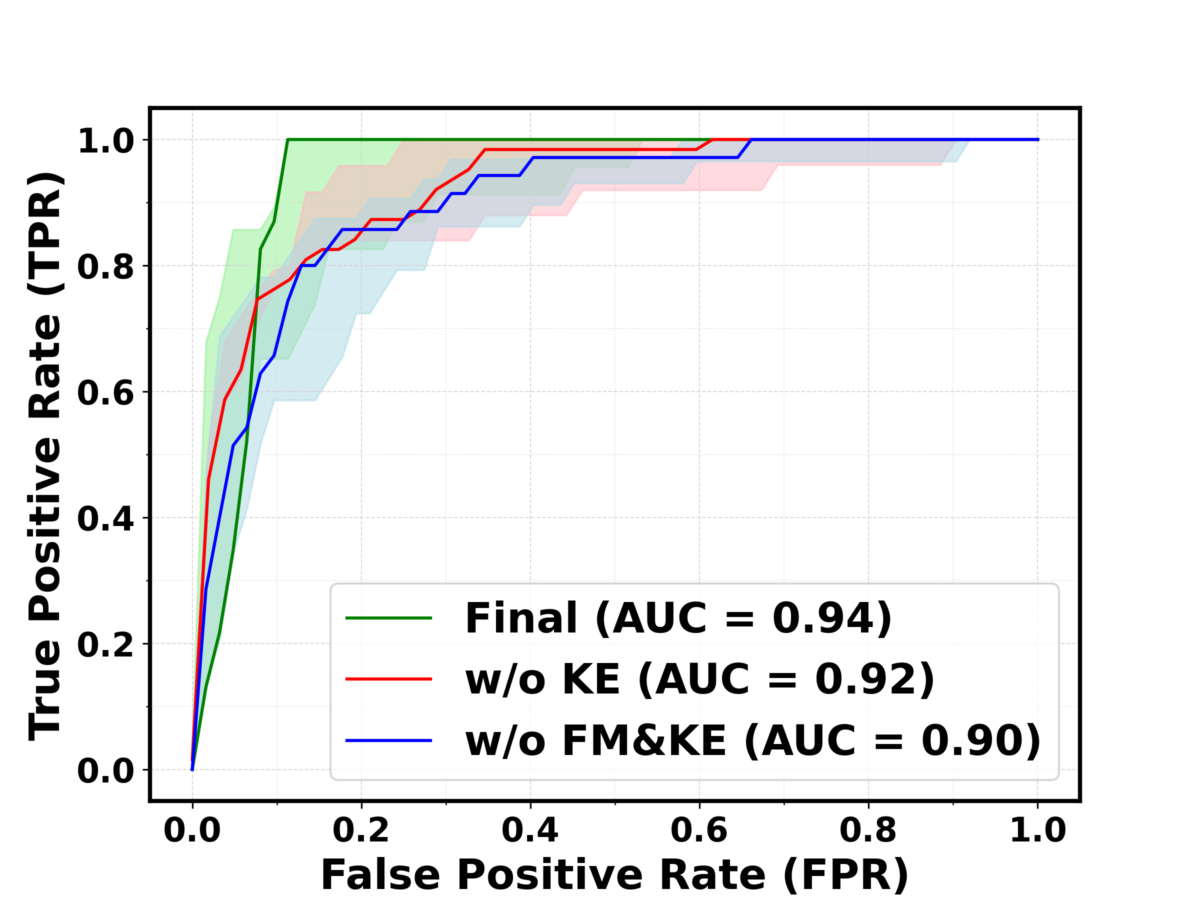
(a) ROCs on Disorders (Head).

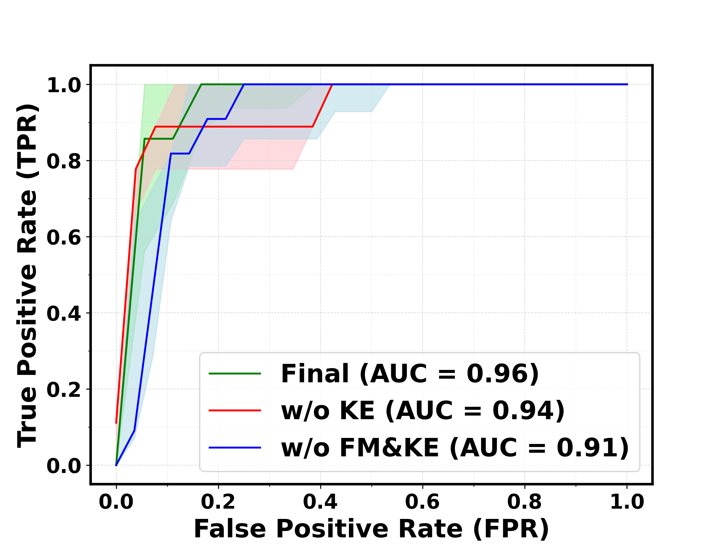
(b) ROCs on Disorders (Medium).

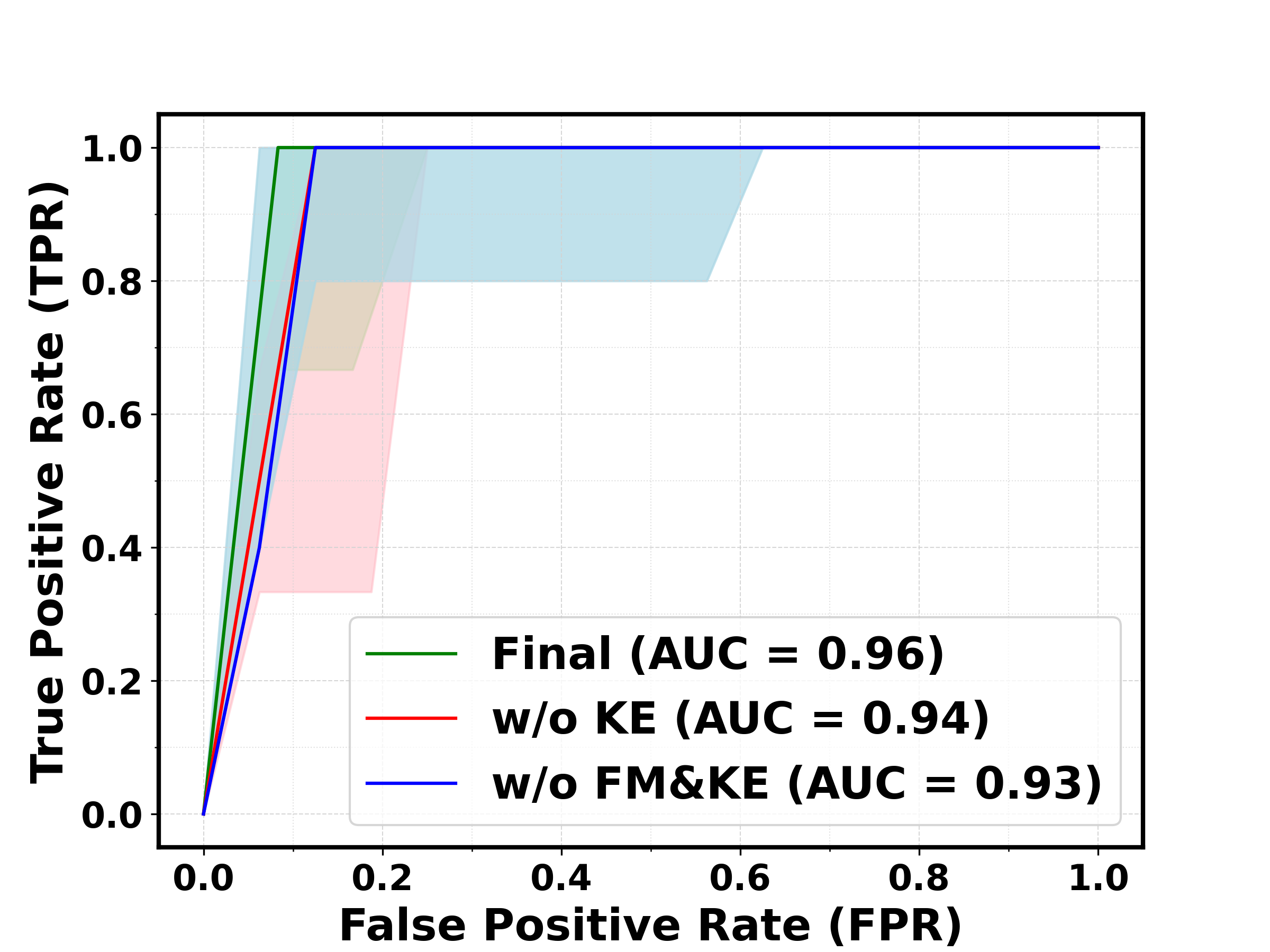
(c) ROCs on Disorders (Tail).

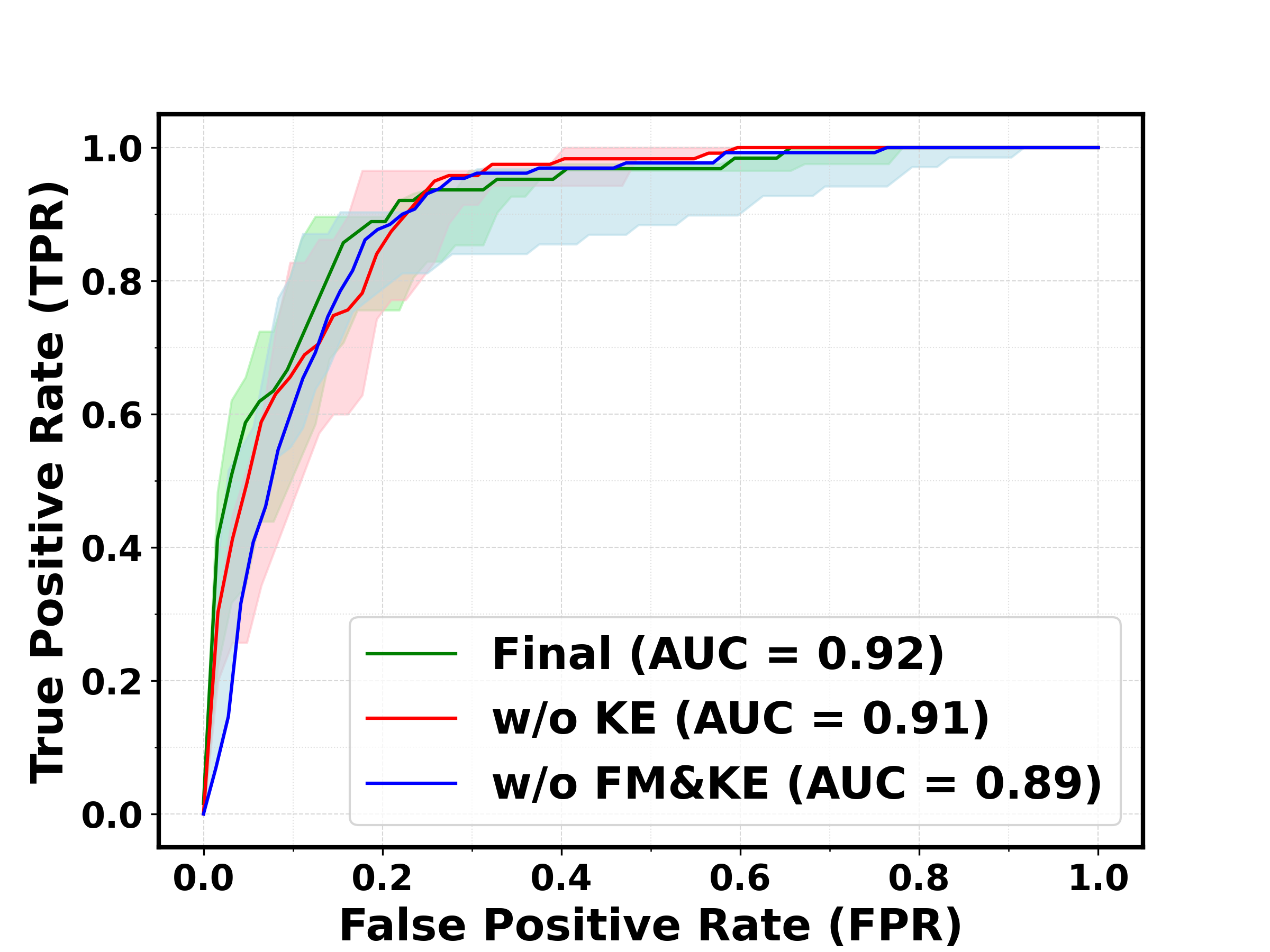
(d) ROCs on ICD-10-CM (Head).

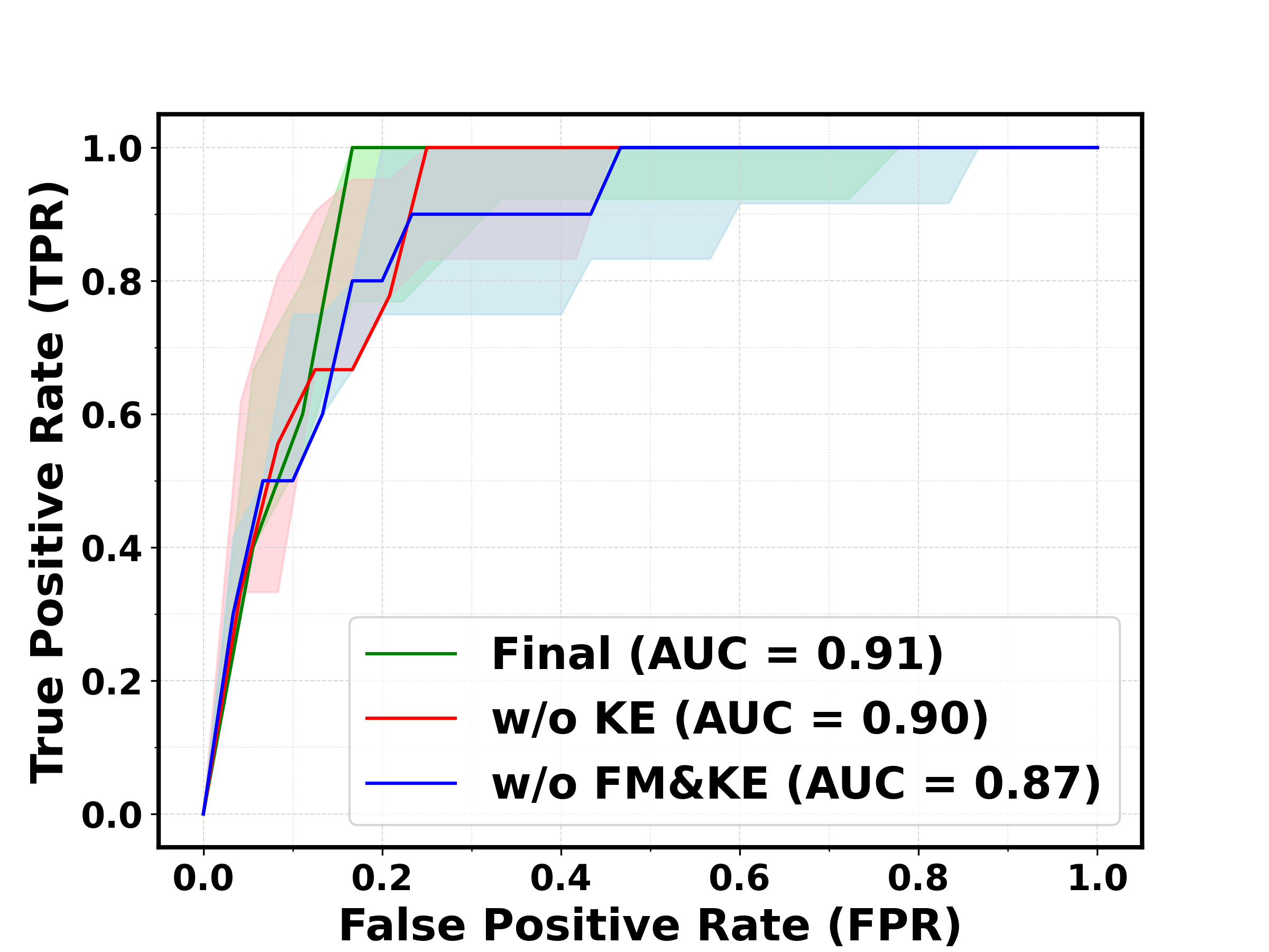
(e) ROCs on ICD-10-CM (Medium).

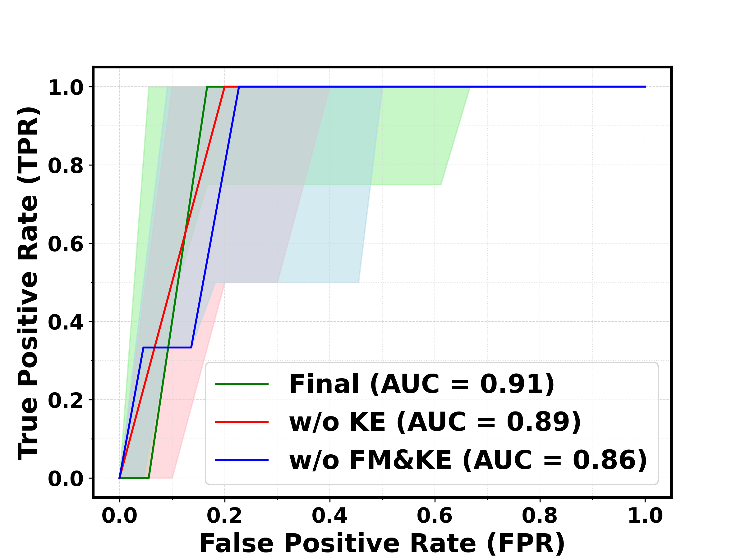
(f) ROCs on ICD-10-CM (Tail).

Figure 7: ROC curves on Disorders and ICD-10-CM, including head/medium/tail parts respectively. The shadow in the figure shown the 95% CI (Confidence interval) and FM, KE are short for Fusion Module and Knowledge Enhancement.

Discussion on Fusion Module. To demonstrate the effectiveness of fusion module, we start with a baseline without FM or KE. As shown in Table 5, adding the fusion module can greatly improve the results on Head, Medium and Tail classes at both disorder and ICD-10-CM levels, showing the critical role for case-level information fusion in diagnosis task. These results align well with our expectations. In clinical practice, the examination of one modality for a diagnosis is often insufficient. A thorough and meticulous diagnostic process typically involves an integrated review of all test results. Each test is weighted differently, depending on how its results correspond with other tests. Our fusion model adeptly mirrors this comprehensive approach, demonstrating its effectiveness in simulating the nuanced process of clinical diagnosis.

Discussion on Knowledge Enhancement. As shown in Table 5, incorporating knowledge enhancement further promotes the final diagnosis performance on both disorder and ICD-10-CM cases, validating the assumption that a better text embedding space trained by rich domain knowledge can greatly help the visual representation learning.

Discussion on ROC Curves. The solid lines in the Figure 7 represents the median AUC value. This value is derived from a process where, for each category, 1000 random samples are taken and the median AUC value is calculated. This procedure is repeated multiple times (1000), with the final curve representing the median of these values. The ROC curve is illustrated by thess solid lines. Accompanying each solid lines is shaded area, which denotes the 95% confidence interval (CI). For each type of implementation, this shaded area is significantly higher than the portion above the solid line. This implies that the AUC value represented by the solid line is generally higher than the class-wise average across different data splits. As shown in the figure, the highest AUC value has reached 0.96, and the lowest value is 0.86, this observed pattern suggests, there exists a few categories that are more challenging to learn than others.

[t] The AUC Score Comparison on Various External Datasets. For each dataset, we carry out experiments with different training data portions, denoted as 1% to 100% in the table. For example, 30% represents we use 30% of data in the downstream training set for finetuning our model or training from scratch. “SOTA” denotes the best performance of former works (pointed with corresponding reference) on the datasets. We mark the gap between ours and training from screatch on the subscript of uparrows$\uparrow$ in the table. Dataset 1% 10% 30% 100% SOTA Scratch Ours Scratch Ours Scratch Ours Scratch Ours VinDr-Mammo 57.05 58.44$\uparrow^{1.39}$ 58.22 59.21$\uparrow^{0.99}$ 62.10 63.11$\uparrow^{1.01}$ 76.25 78.53$\uparrow^{2.28}$ 77.50* [8] CXR14 76.85 79.08$\uparrow^{2.23}$ 77.93 81.72$\uparrow^{3.79}$ 78.52 82.39$\uparrow^{3.87}$ 79.12 83.38$\uparrow^{4.26}$ 82.50* [84] VinDr-Spine 79.35 81.58$\uparrow^{2.23}$ 85.02 86.64$\uparrow^{1.62}$ 86.90 87.21$\uparrow^{0.31}$ 87.35 87.73$\uparrow^{0.38}$ 88.90* [79] MosMedData 52.63 61.33$\uparrow^{8.70}$ 60.72 63.36$\uparrow^{2.64}$ 64.23 69.57$\uparrow^{5.34}$ 71.24 75.39$\uparrow^{4.15}$ 68.47 [57] ADNI 55.39 59.41$\uparrow^{4.02}$ 60.32 64.19$\uparrow^{3.87}$ 63.26 65.77$\uparrow^{2.51}$ 82.40 84.21$\uparrow^{1.81}$ 79.34 [41]

• The numbers are borrowed from the referred papers. We are strictly align with them in train and test split.

6.3 External Evaluation

In this section, we explore the transferring ability of our final model, where we finetune the model on different downstream datasets across various imaging modalities, anatomies and target classes. As shown in Table 6.2, we can see significant performance improvement on various datasets with different data portions, compring to models trained from scratch. Additionally, in most cases, our model can also surpass former SOTAs significantly without any task-specific designs, e.g., architectures, loss functions, demonstrating that our RP3D-DiagDS can also serve as a superior large-scale supervised pre-training dataset for medical domain.

7 Clinical Impact

In this paper, we consider the problem of multi-modality, multi-anatomy, long-tailed disease diagnosis, which has great practical clinical meanings.

First, in clinical practice, patients may get multiple radiologic examinations during their long-term treatment progress from various medical departments. However, existing work on disease classification accepting one image scan, can hardly handle such circumstance, hindering the development of accurate and comprehensive diagnostic models. Our work compensate this and better meet the practical scenarios.

Second, comparing with existing diagnosis works that focus on common general disease classes, our efforts on long-tailed rare classes are more vital for clinical usage. For common diseases, AI diagnosis system, usually, can only help accelerate diagnosis procedure for clinicians, while the hint on rare classes is also critical.

Third, our final model can support finetuning on external diagnosis task. In clinical application, local medical centers can leverage this superiority even with a few training samples. This is remarkable especially considering that, for rare diseases, only a very few cases could be accessible in reality.

8 Limitation

Despite the effectiveness of our proposed dataset, and architecture, there remains some improvements: First, on model design, in fusion step, we can use more image tokens to represent a scan rather than a pooled single vector. The latter may lead to excessive loss of image information during fusion. The model size can be further increased to investigate the effect of model capacities; Second, new loss functions should be explored to tackle such large-scale, long-tailed disorder/disease classification task. Third, on disorder to ICD-10-CM mapping progress, the annotators are labeled on class-name level, i.e., only disorder names are provided, causing some ambiguous classes unable to find strict corresponding ICD-10-CM codes. Though we mark out this class in our shared data files, if providing more case-level information, the mapping could be more accurate. We treat these as future work.

9 Conclusion

In this paper, we focus on solving the problem of multi-modal, multi-label long-tailed case-level diagnosis task. Specifically, we propose a new large-scale diagnosis dataset, namely, RP3D-DiagDS, with 39,026 cases (192,675 scans) labeled with detailed disorders covering 930 ICD-10-CM. On model design, we propose one unified architecture that supports both 2D and 3D input, together with a fusion module, to integrate information from multiple scans of one patient. Additionally, we adopt knowledge enhancement training strategy, leveraging the rich medical domain knowledge to improve the radiologic diagnosis performance. Our final train model also shows strong transferring ability to various external datasets regardless of their imaging modalities, shooting anatomies and target classes. We believe this work can serve as a transition phase between the specialist and generalist models, offering a more feasible and targeted playground for exploring sophisticated algorithms in academia labs, providing a unique opportunity for detailed error analysis, which is often impractical in the development of large-scale generalist models due to prohibitive computational costs.

10 Data and Code Availability

Our dataset RP3D-DiagDS can be found in https://huggingface.co/datasets/QiaoyuZheng/RP3D-DiagDS and our codes can be found in https://github.com/qiaoyu-zheng/RP3D-Diag

11 Supplementary

In this part, we will discuss the baseline implementation in detail. Since most existing architectures cannot perform case-level diagnosis, we propose three parameter-free methods to give case-level prediction with a scan-level classifier:

• Random Picking. We randomly select an image scan a case. It is based on the belief that each scan in a case should encompass the essential information required for an accurate.

• Max Pooling. We adopt max pooling on all the images in a case to get the final prediction. It is based on the principle that if there is an image within a case that can illustrate the presence of abnormality, we should consider it as an unhealthy case.

• Mean Pooling. Instead of max pooling, we replace it with mean pooling in this case. It is rooted in the notion that relying solely on the diagnosis from a single image is insufficient, and our goal is to comprehensively leverage all the scan image information in a case.

Subsequently, we will present a comparative analysis of the outcomes obtained through these strategies, focusing on the two classification standards, ICD-10-CM and disorders, in order to pick out the most powerful baselines for comparison.

Table 6: Results on ICD10-CM classes. We report the different scores for Head/Medium/Tail classes, “Rand”, “Max”. “Mean” represent the random picking, Max Pooling and Mean Pooling respectively.

Granularity	Split	Mode	Metrics
			AUC	AP	F1	MCC	R@0.01	R@0.05	R@0.1
ICD-10-CM	Head	Rand	89.12	12.39	20.51	21.72	24.12	51.82	67.93
		Max	90.39	12.80	20.65	21.94	24.39	54.12	70.11
		Mean	85.49	13.05	20.25	21.52	24.31	49.92	65.28
	Medium	Rand	88.98	7.72	15.44	18.02	22.52	50.50	63.96
		Max	90.15	7.74	15.41	17.96	22.75	51.10	66.31
		Mean	85.05	7.69	15.03	17.53	22.58	47.41	64.52
	Tail	Rand	86.41	4.46	8.54	12.48	8.37	23.74	37.12
		Max	86.46	2.90	6.09	10.27	8.51	25.06	42.80
		Mean	81.50	2.68	5.42	9.04	6.15	20.13	30.64

Table 7: Results on Disorder classes. We report the different scores for Head/Medium/Tail classes, “Rand”, “Max”. “Mean” represent the random picking, Max Pooling and Mean Pooling respectively.

Granularity	Split	Mode	Metrics
			AUC	AP	F1	MCC	R@0.01	R@0.05	R@0.1
Disorders	Head	Rand	91.32	14.08	22.93	24.61	30.68	58.78	73.79
		Max	91.91	13.56	22.08	23.66	30.88	60.50	74.70
		Mean	88.72	14.29	23.26	24.60	31.97	59.67	71.22
	Medium	Rand	92.63	9.47	17.62	20.61	28.18	57.04	71.42
		Max	93.62	9.19	17.16	20.42	28.24	59.32	73.80
		Mean	90.97	9.54	17.33	20.42	29.31	58.15	71.00
	Tail	Rand	87.61	4.85	8.66	13.26	8.58	24.25	41.39
		Max	88.55	4.34	8.03	12.96	9.13	27.46	41.43
		Mean	84.50	4.35	8.09	12.80	9.38	25.96	42.57

As shown in the Table 6 and Table 7, in most cases “Max Pooling” outperform others. Thus in the main body, we all adopt max pooling as our baseline for comparison.

References

- [1] ICD10. https://www.icd10data.com/ICD10CM/Codes.
- [2] Kaggle: Brain mri scans for brain tumor classification. https://www.kaggle.com/datasets/shreyag1103/brain-mri-scans-for-brain-tumor-classification.
- [3] Kaggle: Brain tumor mri dataset. https://www.kaggle.com/dsv/2645886.
- [4] Kaggle: Brain tumor mri images 17 classes. https://www.kaggle.com/datasets/fernando2rad/brain-tumor-mri-images-17-classes.
- [5] Radiopaedia. https://radiopaedia.org.
- [6] Walid Al-Dhabyani, Mohammed Gomaa, Hussien Khaled, and Aly Fahmy. Dataset of breast ultrasound images. Data In Brief, 28:104863, 2020.
- [7] Samuel G Armato III, Geoffrey McLennan, Luc Bidaut, Michael F McNitt-Gray, Charles R Meyer, Anthony P Reeves, Binsheng Zhao, Denise R Aberle, Claudia I Henschke, Eric A Hoffman, et al. The lung image database consortium (lidc) and image database resource initiative (idri): a completed reference database of lung nodules on ct scans. Medical Physics, 38(2):915–931, 2011.
- [8] Sheethal Bhat, Awais Mansoor, Bogdan Georgescu, Adarsh B Panambur, Florin C Ghesu, Saahil Islam, Kai Packhäuser, Dalia Rodríguez-Salas, Sasa Grbic, and Andreas Maier. Aucreshaping: improved sensitivity at high-specificity. Scientific Reports, 13(1):21097, 2023.
- [9] Nicholas Bien, Pranav Rajpurkar, Robyn L Ball, Jeremy Irvin, Allison Park, Erik Jones, Michael Bereket, Bhavik N Patel, Kristen W Yeom, Katie Shpanskaya, et al. Deep-learning-assisted diagnosis for knee magnetic resonance imaging: Development and retrospective validation of mrnet. PLoS Medicine, 15(11), 2018.
- [10] Jannis Born, Gabriel Brändle, Manuel Cossio, Marion Disdier, Julie Goulet, Jérémie Roulin, and Nina Wiedemann. POCOVID-Net: automatic detection of COVID-19 from a new lung ultrasound imaging dataset (POCUS). arXiv preprint arXiv:2004.12084, 2020.
- [11] Andrew P Bradley. The use of the area under the roc curve in the evaluation of machine learning algorithms. Pattern Recognition, 30(7):1145–1159, 1997.
- [12] Aurelia Bustos, Antonio Pertusa, Jose-Maria Salinas, and Maria de la Iglesia-Vayá. Padchest: A large chest x-ray image dataset with multi-label annotated reports. Medical Image Analysis, 66:101797, 2020.
- [13] Charmaine Butt, Jagpal Gill, David Chun, and Benson A Babu. Deep learning system to screen coronavirus disease 2019 pneumonia. Applied Intelligence (Dordrecht, Netherlands), page 1, 2020.
- [14] Hongmin Cai, Qinjian Huang, Wentao Rong, Yan Song, Jiao Li, Jinhua Wang, Jiazhou Chen, Li Li, et al. Breast microcalcification diagnosis using deep convolutional neural network from digital mammograms. Computational and Mathematical Methods in Medicine, 2019, 2019.
- [15] Kai Cao et al. Large-scale pancreatic cancer detection via non-contrast ct and deep learning. Nature Medicine, 2023.
- [16] M Jorge Cardoso, Wenqi Li, Richard Brown, Nic Ma, Eric Kerfoot, Yiheng Wang, Benjamin Murrey, Andriy Myronenko, Can Zhao, Dong Yang, et al. Monai: An open-source framework for deep learning in healthcare. arXiv preprint arXiv:2211.02701, 2022.
- [17] Jun Cheng, Wei Huang, Shuangliang Cao, Ru Yang, Wei Yang, Zhaoqiang Yun, Zhijian Wang, and Qianjin Feng. Enhanced performance of brain tumor classification via tumor region augmentation and partition. PloS One, 10(10):e0140381, 2015.
- [18] Davide Chicco and Giuseppe Jurman. The advantages of the matthews correlation coefficient (mcc) over f1 score and accuracy in binary classification evaluation. BMC Genomics, 21(1):1–13, 2020.
- [19] Muhammad EH Chowdhury, Tawsifur Rahman, Amith Khandakar, Rashid Mazhar, Muhammad Abdul Kadir, Zaid Bin Mahbub, Khandakar Reajul Islam, Muhammad Salman Khan, Atif Iqbal, Nasser Al Emadi, et al. Can ai help in screening viral and covid-19 pneumonia? IEEE Access, 8:132665–132676, 2020.
- [20] Yin Dai, Yifan Gao, and Fayu Liu. Transmed: Transformers advance multi-modal medical image classification. Diagnostics, 11(8):1384, 2021.
- [21] S Deepak and PM Ameer. Brain tumor classification using deep cnn features via transfer learning. Computers in Biology and Medicine, 111:103345, 2019.
- [22] Dina Demner-Fushman, Marc D Kohli, Marc B Rosenman, Sonya E Shooshan, Laritza Rodriguez, Sameer Antani, George R Thoma, and Clement J McDonald. Preparing a collection of radiology examinations for distribution and retrieval. Journal of the American Medical Informatics Association, 23(2):304–310, 2016.
- [23] Alexey Dosovitskiy, Lucas Beyer, Alexander Kolesnikov, Dirk Weissenborn, Xiaohua Zhai, Thomas Unterthiner, Mostafa Dehghani, Matthias Minderer, Georg Heigold, Sylvain Gelly, et al. An image is worth 16x16 words: Transformers for image recognition at scale. arXiv preprint arXiv:2010.11929, 2020.
- [24] Andrew Estabrooks, Taeho Jo, and Nathalie Japkowicz. A multiple resampling method for learning from imbalanced data sets. Computational Intelligence, 20(1):18–36, 2004.
- [25] Ross W Filice, Anouk Stein, Carol C Wu, Veronica A Arteaga, Stephen Borstelmann, Ramya Gaddikeri, et al. Crowdsourcing pneumothorax annotations using machine learning annotations on the nih chest x-ray dataset. Journal of Digital Imaging, 33:490–496, 2020.
- [26] Xiaohong Gao, Yu Qian, and Alice Gao. COVID-VIT: Classification of COVID-19 from CT chest images based on vision transformer models. arXiv preprint arXiv:2107.01682, 2021.
- [27] Behnaz Gheflati and Hassan Rivaz. Vision transformers for classification of breast ultrasound images. In 2022 44th Annual International Conference of the IEEE Engineering in Medicine & Biology Society (EMBC), pages 480–483. IEEE, 2022.
- [28] Agrim Gupta, Piotr Dollar, and Ross Girshick. Lvis: A dataset for large vocabulary instance segmentation. In Proceedings of the IEEE/CVF Conference on Computer Vision and Pattern Recognition (CVPR), June 2019.
- [29] Akila Gurunathan and Batri Krishnan. A hybrid cnn-glcm classifier for detection and grade classification of brain tumor. Brain Imaging and Behavior, 16(3):1410–1427, 2022.
- [30] Kaiming He, X. Zhang, Shaoqing Ren, and Jian Sun. Deep residual learning for image recognition. 2016 IEEE Conference on Computer Vision and Pattern Recognition (CVPR), pages 770–778, 2015.
- [31] JF Healthcare. Object-CXR - Automatic detection of foreign objects on chest X-rays. 2020.
- [32] Heath, Michael and Bowyer, Kevin and Kopans, Daniel, and Moore, Richard and Kegelmeyer, W. Philip. The digital database for screening mammography. In Proceedings of the Fifth International Workshop on Digital Mammography, pages 212–218. Medical Physics Publishing, 2001.
- [33] Murtadha D. Hssayeni, Muayad S. Croock, Aymen D. Salman, Hassan Falah Al-khafaji, Zakaria A. Yahya, and Behnaz Ghoraani. Intracranial hemorrhage segmentation using a deep convolutional model. Data, 5(1), 2020.
- [34] Jeremy Irvin, Pranav Rajpurkar, Michael Ko, Yifan Yu, Silviana Ciurea-Ilcus, Chris Chute, Henrik Marklund, Behzad Haghgoo, Robyn Ball, Katie Shpanskaya, et al. CheXpert: A Large Chest Radiograph Dataset with Uncertainty Labels and Expert Comparison. In Proceedings of the AAAI Conference on Artificial Intelligence, volume 33, pages 590–597, 2019.
- [35] Clifford R Jack Jr, Matt A Bernstein, Nick C Fox, Paul Thompson, Gene Alexander, Danielle Harvey, Bret Borowski, Paula J Britson, Jennifer L. Whitwell, Chadwick Ward, et al. The alzheimer’s disease neuroimaging initiative (adni): Mri methods. Journal of Magnetic Resonance Imaging: An Official Journal of the International Society for Magnetic Resonance in Medicine, 27(4):685–691, 2008.
- [36] Stefan Jaeger, Sema Candemir, Sameer Antani, Yì-Xiáng J Wáng, Pu-Xuan Lu, and George Thoma. Two public chest x-ray datasets for computer-aided screening of pulmonary diseases. Quantitative Imaging in Medicine and Surgery, 4(6):475, 2014.
- [37] Qiao Jin, Won Kim, Qingyu Chen, Donald C Comeau, Lana Yeganova, W John Wilbur, and Zhiyong Lu. Medcpt: Contrastive pre-trained transformers with large-scale pubmed search logs for zero-shot biomedical information retrieval. Bioinformatics, 39(11):btad651, 2023.
- [38] Alistair EW Johnson, Tom J Pollard, Seth J Berkowitz, Nathaniel R Greenbaum, Matthew P Lungren, Chih-ying Deng, Roger G Mark, and Steven Horng. Mimic-cxr, a de-identified publicly available database of chest radiographs with free-text reports. Scientific Data, 6(1):317, 2019.
- [39] Lauren N. Koenig, Gregory S. Day, Amber Salter, Sarah Keefe, Laura M. Marple, Justin Long, Pamela LaMontagne, Parinaz Massoumzadeh, B. Joy Snider, Manasa Kanthamneni, Cyrus A. Raji, Nupur Ghoshal, Brian A. Gordon, Michelle Miller-Thomas, John C. Morris, Joshua S. Shimony, and Tammie L.S. Benzinger. Select atrophied regions in alzheimer disease (sara): An improved volumetric model for identifying alzheimer disease dementia. NeuroImage: Clinical, 26:102248, 2020.
- [40] Dimitrios Kollias, Anastasios Arsenos, Levon Soukissian, and Stefanos Kollias. Mia-cov19d: Covid-19 detection through 3-d chest ct image analysis. In Proceedings of the IEEE/CVF International Conference on Computer Vision, pages 537–544, 2021.
- [41] S Korolev, A Safiullin, M Belyaev, and Y Dodonova. Residual and plain convolutional neural networks for 3D brain MRI classification. In Proceedings-International Symposium on Biomedical Imaging, pages 835–838, 2017.
- [42] Michał Koziarski. Radial-based undersampling for imbalanced data classification. Pattern Recognition, 102:107262, 2020.
- [43] Pamela J. LaMontagne, Tammie LS. Benzinger, John C. Morris, Sarah Keefe, Russ Hornbeck, Chengjie Xiong, Elizabeth Grant, Jason Hassenstab, Krista Moulder, Andrei G. Vlassenko, Marcus E. Raichle, Carlos Cruchaga, and Daniel Marcus. Oasis-3: Longitudinal neuroimaging, clinical, and cognitive dataset for normal aging and alzheimer disease. medRxiv, 2019.
- [44] Rebecca Sawyer Lee, Francisco Gimenez, Assaf Hoogi, Kanae Kawai Miyake, Mia Gorovoy, and Daniel L Rubin. A curated mammography data set for use in computer-aided detection and diagnosis research. Scientific Data, 4(1):1–9, 2017.
- [45] Bo Li, Yongqiang Yao, Jingru Tan, Gang Zhang, Fengwei Yu, Jianwei Lu, and Ye Luo. Equalized focal loss for dense long-tailed object detection. In Proceedings of the IEEE/CVF Conference on Computer Vision and Pattern Recognition (CVPR), pages 6990–6999, 2022.
- [46] Lin Li, Lixin Qin, Zeguo Xu, Youbing Yin, Xin Wang, Bin Kong, Junjie Bai, Yi Lu, Zhenghan Fang, Qi Song, et al. Artificial intelligence distinguishes COVID-19 from community acquired pneumonia on chest CT. Radiology, 2020.
- [47] Tsung-Yi Lin, Priya Goyal, Ross B. Girshick, Kaiming He, and Piotr Dollár. Focal loss for dense object detection. IEEE International Conference on Computer Vision (ICCV), pages 2999–3007, 2017.
- [48] Chengeng Liu and Qingshan Yin. Automatic diagnosis of covid-19 using a tailored transformer-like network. In Journal of Physics: Conference Series, volume 2010, page 012175. IOP Publishing, 2021.
- [49] Xu-Ying Liu, Jianxin Wu, and Zhi-Hua Zhou. Exploratory undersampling for class-imbalance learning. IEEE Transactions on Systems, Man, and Cybernetics, Part B (Cybernetics), 39(2):539–550, 2008.
- [50] Anna Majkowska et al. Chest radiograph interpretation with deep learning models: assessment with radiologist-adjudicated reference standards and population-adjusted evaluation. Radiology, 294(2):421–431, 2020.
- [51] Daniel S. Marcus, Tracy H. Wang, Jamie Parker, John G. Csernansky, John C. Morris, and Randy L. Buckner. Open Access Series of Imaging Studies (OASIS): Cross-sectional MRI Data in Young, Middle Aged, Nondemented, and Demented Older Adults. Journal of Cognitive Neuroscience, 19(9):1498–1507, 09 2007.
- [52] Christos Matsoukas, Johan Fredin Haslum, Magnus Söderberg, and Kevin Smith. Is it time to replace cnns with transformers for medical images? arXiv preprint arXiv:2108.09038, 2021.
- [53] Xueyan Mei, Zelong Liu, Philip M Robson, Brett Marinelli, Mingqian Huang, Amish Doshi, Adam Jacobi, Chendi Cao, Katherine E Link, Thomas Yang, et al. Radimagenet: an open radiologic deep learning research dataset for effective transfer learning. Radiology: Artificial Intelligence, 4(5):e210315, 2022.
- [54] Taylor R Moen, Baiyu Chen, David R Holmes III, Xinhui Duan, Zhicong Yu, Lifeng Yu, Shuai Leng, Joel G Fletcher, and Cynthia H McCollough. Low-dose ct image and projection dataset. Medical Physics, 48(2):902–911, 2021.
- [55] Arnab Kumar Mondal, Arnab Bhattacharjee, Parag Singla, and AP Prathosh. xViTCOS: explainable vision transformer based COVID-19 screening using radiography. IEEE Journal of Translational Engineering in Health and Medicine, 10:1–10, 2021.
- [56] Michael Moor, Qian Huang, Shirley Wu, Michihiro Yasunaga, Cyril Zakka, Yash Dalmia, Eduardo Pontes Reis, Pranav Rajpurkar, and Jure Leskovec. Med-Flamingo: A Multimodal Medical Few-shot Learner. arXiv preprint arXiv:2307.15189, July 2023.
- [57] Sergey P Morozov, AE Andreychenko, NA Pavlov, AV Vladzymyrskyy, NV Ledikhova, VA Gombolevskiy, Ivan A Blokhin, PB Gelezhe, AV Gonchar, and V Yu Chernina. Mosmeddata: Chest ct scans with covid-19 related findings dataset. arXiv preprint arXiv:2005.06465, 2020.
- [58] Sayyed Mostafa Mostafavi. COVID19-CT-Dataset: An Open-Access Chest CT Image Repository of 1000+ Patients with Confirmed COVID-19 Diagnosis. 2021.
- [59] Ha Q Nguyen, Khanh Lam, Linh T Le, Hieu H Pham, Dat Q Tran, Dung B Nguyen, et al. VinDr-CXR: An open dataset of chest X-rays with radiologist’s annotations. Scientific Data, 9(1):429, 2022.
- [60] Hieu T Nguyen, Ha Q Nguyen, Hieu H Pham, Khanh Lam, Linh T Le, Minh Dao, and Van Vu. VinDr-Mammo: A large-scale benchmark dataset for computer-aided diagnosis in full-field digital mammography. Scientific Data, 10(1):277, 2023.
- [61] Hieu T. Nguyen, Ha Q. Nguyen, H. H. Pham, Khanh Lam, L. T. Le, M. Dao, and Van H. Vu. VinDr-Mammo: A large-scale benchmark dataset for computer-aided diagnosis in full-field digital mammography. PhysioNet, 2022.
- [62] Hieu T Nguyen, Hieu H Pham, Nghia T Nguyen, Ha Q Nguyen, Thang Q Huynh, Minh Dao, and Van Vu. VinDr-SpineXR: A deep learning framework for spinal lesions detection and classification from radiographs. In Medical Image Computing and Computer Assisted Intervention–MICCAI 2021: 24th International Conference, Strasbourg, France, September 27–October 1, 2021, Proceedings, Part V 24, pages 291–301. Springer, 2021.
- [63] Ngoc Hung Nguyen, Hieu Pham, Thanh-Truong Tran, Tuan Ngoc Minh Nguyen, and Ha Q. Nguyen. VinDr-PCXR: An open, large-scale chest radiograph dataset for interpretation of common thoracic diseases in children. PhysioNet, 2022.
- [64] OpenAI. GPT-4 Technical Report. arXiv preprint arXiv:2303.08774, 2023.
- [65] Sangjoon Park, Gwanghyun Kim, Yujin Oh, Joon Beom Seo, Sang Min Lee, Jin Hwan Kim, Sungjun Moon, Jae-Kwang Lim, and Jong Chul Ye. Vision transformer for covid-19 cxr diagnosis using chest x-ray feature corpus. arXiv preprint arXiv:2103.07055, 2021.
- [66] Maya Pavlova et al. Covid-net cxr-2: An enhanced deep convolutional neural network design for detection of covid-19 cases from chest x-ray images. Frontiers in Medicine, 9, 2022.
- [67] Shehan Perera, Srikar Adhikari, and Alper Yilmaz. Pocformer: A lightweight transformer architecture for detection of covid-19 using point of care ultrasound. In 2021 IEEE international conference on image processing (ICIP), pages 195–199. IEEE, 2021.
- [68] Tal Ridnik, Emanuel Ben-Baruch, Nadav Zamir, Asaf Noy, Itamar Friedman, Matan Protter, and Lihi Zelnik-Manor. Asymmetric loss for multi-label classification. In Proceedings of the IEEE/CVF International Conference on Computer Vision, pages 82–91, 2021.
- [69] Muhammad Sajjad, Salman Khan, Khan Muhammad, Wanqing Wu, Amin Ullah, and Sung Wook Baik. Multi-grade brain tumor classification using deep cnn with extensive data augmentation. Journal of Computational Science, 30:174–182, 2019.
- [70] Zhuchen Shao, Hao Bian, Yang Chen, Yifeng Wang, Jian Zhang, Xiangyang Ji, et al. TransMIL: Transformer based Correlated Multiple Instance Learning for Whole Slide Image Classification. Advances in Neural Information Processing Systems, 34:2136–2147, 2021.
- [71] George Shih, Carol C Wu, Safwan S Halabi, Marc D Kohli, Luciano M Prevedello, et al. Augmenting the national institutes of health chest radiograph dataset with expert annotations of possible pneumonia. Radiology: Artificial Intelligence, 1(1):e180041, 2019.
- [72] Debaditya Shome, T Kar, Sachi Nandan Mohanty, Prayag Tiwari, Khan Muhammad, Abdullah AlTameem, Yazhou Zhang, and Abdul Khader Jilani Saudagar. Covid-transformer: Interpretable covid-19 detection using vision transformer for healthcare. International Journal of Environmental Research and Public Health, 18(21):11086, 2021.
- [73] Zar Nawab Khan Swati, Qinghua Zhao, Muhammad Kabir, Farman Ali, Zakir Ali, Saeed Ahmed, and Jianfeng Lu. Brain tumor classification for mr images using transfer learning and fine-tuning. Computerized Medical Imaging and Graphics, 75:34–46, 2019.
- [74] Youbao Tang, Ke Yan, Jing Xiao, and Ronald M Summers. One click lesion recist measurement and segmentation on ct scans. In Medical Image Computing and Computer Assisted Intervention (MICCAI), 2020.
- [75] Tao Tu, Shekoofeh Azizi, Danny Driess, Mike Schaekermann, Mohamed Amin, Pi-Chuan Chang, Andrew Carroll, Chuck Lau, Ryutaro Tanno, Ira Ktena, et al. Towards generalist biomedical ai. arXiv preprint arXiv:2307.14334, 2023.
- [76] Xiaosong Wang, Yifan Peng, Le Lu, Zhiyong Lu, Mohammadhadi Bagheri, and Ronald M Summers. Chestx-ray8: Hospital-scale chest x-ray database and benchmarks on weakly-supervised classification and localization of common thorax diseases. In Proceedings of the IEEE/CVF Conference on Computer Vision and Pattern Recognition (CVPR), pages 2097–2106, 2017.
- [77] Xuezhi Wang, Jason Wei, Dale Schuurmans, Quoc Le, Ed Chi, Sharan Narang, Aakanksha Chowdhery, and Denny Zhou. Self-consistency improves chain of thought reasoning in language models. arXiv preprint arXiv:2203.11171, 2022.
- [78] Chaoyi Wu, Feng Chang, Xiao Su, Zhihan Wu, Yanfeng Wang, Ling Zhu, and Ya Zhang. Integrating features from lymph node stations for metastatic lymph node detection. Computerized medical imaging and graphics : the official journal of the Computerized Medical Imaging Society, 101:102108, 2022.
- [79] Chaoyi Wu, Xiaoman Zhang, Yanfeng Wang, Ya Zhang, and Weidi Xie. K-diag: Knowledge-enhanced disease diagnosis in radiographic imaging. Medical Image Computing and Computer Assisted Intervention – MICCAI Workshop, 2023.
- [80] Chaoyi Wu, Xiaoman Zhang, Ya Zhang, Yanfeng Wang, and Weidi Xie. MedKLIP: Medical Knowledge Enhanced Language-Image Pre-Training. arXiv preprint arXiv:2301.02228, 2023.
- [81] Chaoyi Wu, Xiaoman Zhang, Ya Zhang, Yanfeng Wang, and Weidi Xie. Towards generalist foundation model for radiology by leveraging web-scale 2d&3d medical data. IEEE International Conference on Computer Vision (ICCV), 2023.
- [82] Ke Yan, Xiaosong Wang, Le Lu, and Ronald M Summers. Deeplesion: Automated deep mining, categorization and detection of significant radiology image findings using large-scale clinical lesion annotations. arXiv preprint arXiv:1710.01766, 2017.
- [83] Shuang Yu, Kai Ma, Qi Bi, Cheng Bian, Munan Ning, Nanjun He, Yuexiang Li, Hanruo Liu, and Yefeng Zheng. Mil-vt: Multiple instance learning enhanced vision transformer for fundus image classification. In Medical Image Computing and Computer Assisted Intervention(MICCAI), 2021.
- [84] Xiaoman Zhang, Chaoyi Wu, Ya Zhang, Yanfeng Wang, and Weidi Xie. Knowledge-enhanced pre-training for auto-diagnosis of chest radiology images. Nature Communications, 2023.
- [85] Xiaoman Zhang, Chaoyi Wu, Ziheng Zhao, Weixiong Lin, Ya Zhang, Yanfeng Wang, and Weidi Xie. Pmc-vqa: Visual instruction tuning for medical visual question answering. arXiv preprint arXiv:2305.10415, 2023.
- [86] Yao Zhang, Nanjun He, Jiawei Yang, Yuexiang Li, Dong Wei, Yawen Huang, Yang Zhang, Zhiqiang He, and Yefeng Zheng. mmformer: Multimodal medical transformer for incomplete multimodal learning of brain tumor segmentation. In International Conference on Medical Image Computing and Computer-Assisted Intervention, pages 107–117. Springer, 2022.
- [87] Yi Zheng, Rushin H Gindra, Emily J Green, Eric J Burks, Margrit Betke, Jennifer E Beane, and Vijaya B Kolachalama. A graph-transformer for whole slide image classification. IEEE Transactions on Medical Imaging, 41(11):3003–3015, 2022.