Causal bounds on cosmological angular correlation

Abstract

Causal relationships in conformal geometry are used to analyze angular boundaries of cosmic microwave background (CMB) correlations. It is shown that curvature correlations limited to timelike intervals on world lines that have connected causal diamonds during inflation generate an angular correlation function $C(\Theta)$ of gravitationally-induced CMB anisotropy that vanishes in a range of angular separation from $\Theta=\pi/2-\arcsin(1/4)$ to as far as $\Theta=3\pi/4$. This model-independent symmetry is shown to agree remarkably well with even-parity and dipole-corrected CMB correlations measured in all-sky maps from the WMAP and Planck satellites. Realizations of the standard quantum field theory cosmological model are shown to produce comparably small correlation with probabilities ranging from $\simeq 10^{-4.3}$ to $\simeq 10^{-1.5}$, depending on the map and range of angular separation. These measurements are interpreted as evidence for a causal symmetry based on a basic physical principle not included in the effective field theory approximation to cosmological quantum gravity: quantum fluctuations only generate physical correlations of spacetime curvature within regions bounded by causal diamonds. Theoretical implications and further cosmological tests of this interpretation are briefly discussed.

1 Introduction

In classical cosmology, gravitational potential perturbations on the largest scales at late times approximately preserve the primordial pattern laid down on those scales at the earliest times (Bardeen, 1980). In the context of cosmic inflation, the temperature anisotropy of the cosmic microwave background (CMB) on large angular scales is the most direct measurement of primordial quantum gravitational fluctuations because its pattern since the earliest times has been shaped only by gravity (Sachs & Wolfe, 1967; Hu & Dodelson, 2002).

In spite of this unique significance, CMB correlations at large angles are generally disregarded in precision cosmological tests, primarily because the standard picture of inflation predicts a large variance in possible outcomes. This “cosmic variance” originates from the quantum model used to compute the statistical properties of primordial fluctuations, based on quantum field theory (QFT) (Baumann, 2011): on large scales, the anisotropy is mostly shaped by a small number of long-wavelength modes, with a range of independent amplitudes and phases.

At the same time, the CMB correlation function $C(\Theta)$ over a range of large angular separation $\Theta$ is measured to have absolute values that are anomalously small compared to expected realizations of the QFT model (Bennett et al., 2003; Copi et al., 2009; Bennett et al., 2011; Planck Collaboration, 2016, 2020a; Muir et al., 2018; Hagimoto et al., 2020). This anomaly is customarily interpreted as a statistical fluke, but it could be evidence for a new physical effect, perhaps even a unique indication that QFT does not correctly describe gravitational physics at large length scales.

Indeed, it is known that QFT has foundational theoretical inconsistencies with active gravity on large scales, since, among other issues, causal structure itself is not included as part of the quantum system (Cohen et al., 1999; Hollands & Wald, 2004; Stamp, 2015). Since cosmological curvature perturbations inherit their spatial pattern from quantum fluctuations of gravity on the scale of causal horizons, they are uniquely suited to search for departures from QFT on these scales (Hogan, 2019, 2020).

In previous work (Hogan & Meyer, 2022; Hogan et al., 2023), we used classical models of noise composed of perturbative gravitational shock displacements during inflation to estimate correlations from fluctuations coherent on null surfaces, and compared them with the observed large-scale anisotropy of the CMB. In this paper, we do not model the magnitude of nonzero correlations or the quantum dynamics of fluctuations, but instead use inflationary causal structure to identify a range of angular separation over which correlations are predicted to vanish. This purely geometrical, parameter-free approach is based solely on boundaries of classical causal relationships and a specific hypothesis about the causal boundaries of physical quantum phenomena.

Our hypothesis is that primordial fluctuations are “causally coherent,” in the sense that they only produce nonzero relict correlations within the geometrical boundaries of two-way causal relationships between world lines defined by causal diamonds during inflation. We first describe the basic causal constraints on measurement that motivate this hypothesis. Then, we analyze how boundaries in primordial causal structure map onto angular boundaries of large scale correlation in the CMB, produced by the two main gravitational sources of anisotropy on large angular scales, the Sachs-Wolfe (SW) effect and Integrated Sachs-Wolfe (ISW) effect (Hu & Dodelson, 2002). We show that angular boundaries of causal diamond intersections delimit a new symmetry called a “causal shadow”: the angular correlation function $C(\Theta)$ of perturbations exactly vanishes over a wide range of angular separation $\Theta$ around $\pi/2$,

$$C(\pi/2-\arcsin(1/4)<\Theta<\Theta_{0})=0,$$ (1)

where the outer boundary extends to at least $\Theta_{0}\geq 2\pi/3$ and possibly as far as $\Theta_{0}=3\pi/4$.

Earlier studies are consistent with this new prediction. For example, Hagimoto et al. (2020) found that $C(\Theta)$ in the best Planck maps at $\Theta=\pi/2$ indeed lies in a range remarkably close to zero:

$$-0.22\mu{\rm K}^{2}<C(\Theta=\pi/2)<+2.16\mu{\rm K}^{2},$$ (2)

which indicates that the true correlation is hundreds of times smaller (at least) than the value in typical standard realizations, and closer to zero than all but $0.52\%$ of such realizations.

Up to now, the exact null symmetry predicted over the broad range of $\Theta$ in Eq. (1) has been hidden: because all measured maps have their dipole ($\ell=1$) mode subtracted, the measured correlation differs from its primordial value everywhere except at $\Theta=\pi/2$. In this paper, we extend measurements of the causal shadow to the predicted range of $\Theta$. We implement statistical tests that account for the dipole in a model-independent way, using even-parity and dipole-corrected correlations. Galaxy-subtracted CMB maps are compared with the causal shadow prediction, and with standard inflationary realizations. Our measurements show remarkable agreement with the simple null symmetry described by Eq. (1): departures from zero correlation, which we attribute mostly to errors in Galaxy subtraction, are again orders of magnitude smaller than typical correlations in standard realizations. A rank comparison shows that such small correlations very rarely occur by chance in the standard picture.

We interpret this striking result as a signature of a basic physical principle that leads to a causal constraint on quantum gravitational fluctuations: quantum fluctuations only generate physical correlations of spacetime curvature within causal diamonds. Such a universal causal constraint is not consistent with the standard effective quantum field theory approximation for formation of inflationary perturbations, but could arise from a deeper structure of quantum gravity. The constraint on large-angle correlations would not significantly affect the broadly successful late-time concordance of the standard slow-roll inflationary scenario with smaller-scale CMB anisotropy and large-scale cosmic structure, since it is consistent with the standard prediction of a slightly tilted, direction-averaged 3D power spectrum of curvature perturbations. We briefly discuss further observational tests of this interpretation, and its implications for quantum cosmology and fundamental gravitational theory.

2 Causal relationships

2.1 Conformal causal structure

The standard Friedmann-Lemaître-Robertson-Walker cosmological metric can be written as

$$ds^{2}=a^{2}(t)[c^{2}d\eta^{2}-d\Sigma^{2}],$$ (3)

where $t$ denotes proper cosmic time for any comoving observer, $d\eta\equiv dt/a(t)$ denotes a conformal time interval, $a(t)$ denotes the cosmic scale factor, and the spatial 3-metric in comoving coordinates is

$$d\Sigma^{2}=dr^{2}+r^{2}d\Omega^{2},$$ (4)

where the angular separation $d\Omega$ in standard polar notation satisfies $d\Omega^{2}=d\theta^{2}+\sin^{2}\theta d\phi^{2}$. Light cones and causal diamonds are defined by null relationships in comoving conformal coordinates,

$$d\Sigma=\pm cd\eta.$$ (5)

Thus, in conformal coordinates, cosmological causal relationships are the same as those in flat spacetime. Some key relationships are shown in Figure (1).

2.2 Causal relationships during inflation

Cosmological inflation (Baumann, 2011) was introduced to solve a conceptual problem with initial conditions, sometimes called the “horizon problem”: if the cosmic expansion slows with time ($\ddot{a}<0$), causal connections are only possible over smaller comoving regions in the past, so there is no causal mechanism for generating any kind of correlations in the initial conditions.

Inflation solves the main problem by introducing early cosmic acceleration, so that the comoving causal horizon moves closer with time rather than farther away. If the scale factor $a(t)$ undergoes many orders of magnitude of expansion during early acceleration ($\ddot{a}>0$), even very distant comoving world lines were once in causal contact. This causal relationship is shown in Figs. (1) and (2): given enough inflation, at a sufficiently early time, any comoving world line at finite separation lies within the past light cone of another at the end of inflation, its inflationary horizon ${\cal H}$. A causal connection in principle provides an opportunity to account for the large scale near-uniformity of the universe, as well as large-scale, small amplitude perturbations from quantum fluctuations.

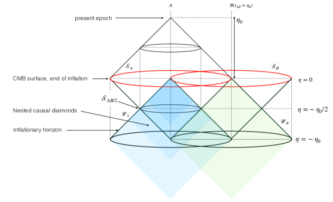
Figure 1: Boundaries of causal relationships and coherent cosmological correlations around a world line in conformal, comoving coordinates. The past light cone of observer $A$ at time $\eta=\eta_{0}$ intersects the end of inflation on a sphere ${\cal S}_{A}$ with radius $r_{AB}=\eta_{0}$. Another world line $B$ lies on ${\cal S}_{A}$. The past light cones of the two world lines at the end of inflation are their inflationary horizons, ${\cal H}_{A}$ and ${\cal H}_{B}$. Each horizon has nested causal diamonds that describe two-way classical causal relationships of outgoing and incoming information, bounded by spherical surfaces of constant conformal time, or “horizon footprints.” A diamond nested within a horizon ${\cal H}$ is posited to bound physical correlations of classical curvature perturbations with its world line interval. The surfaces ${\cal S}_{A}$ and ${\cal S}_{B}$ with radius $\eta_{0}$ intersect their horizons at $\eta=-\eta_{0}$, and encompass the largest causally-generated correlations observable by time $\eta_{0}$. Note the special significance of the causal diamond with radius $\eta_{0}/2$ and bounding surface ${\cal S}_{AB/2}$: subsequent causal diamonds nested in ${\cal H}_{A}$ start outside of ${\cal H}_{B}$, so their frozen fluctuations correlated with $A$ are causally disentangled from and hence uncorrelated with $B$.

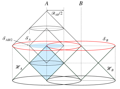
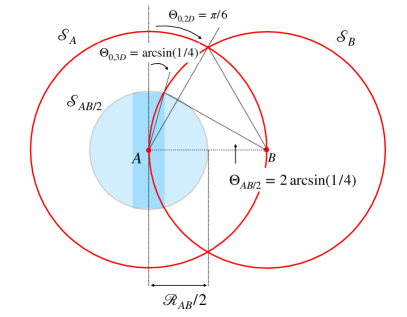
Figure 2: How causal relationship boundaries map onto those of angular correlations. Left panel shows causal relationships as in Fig. (1). A causal diamond of ${\cal H}_{A}$ only intersects ${\cal H}_{B}$ if it has a radius $>{\cal R}_{AB}/2$. Its footprint ${\cal S}_{AB/2}$ is the smallest $A$ footprint entangled with ${\cal H}_{B}$, and thus the minimum radius that produces correlations of any world line with $B$ as measured by $A$. The right panel shows a cross section of corresponding spherical surfaces and the intersections that determine angular boundaries of correlations. The intersection of the two footprints, ${\cal S}_{B}$ and the shaded sphere ${\cal S}_{AB/2}$, occurs at an angle $\Theta=\pi/2-\Theta_{0,\>\!3\text{D}}$ from the $AB$ axis, with $\Theta_{0,\>\!3\text{D}}=\arcsin(1/4)$, which bounds the general 3D causal shadow (Eq. 12). Angular correlations on ${\cal S}_{A}$ itself are bounded by the intersection of ${\cal S}_{A}$ with ${\cal S}_{B}$; this occurs at $\Theta_{0,\>\!2\text{D}}=\pi/6$, the general thin-sphere causal shadow (Eq. 13). The angle $\Theta_{AB/2}$ represents the largest angular separation on ${\cal S}_{B}$ of world lines with a two-way causal connection after they leave ${\cal H}_{B}$ and before the end of inflation (Eq. 25).

2.3 Causal relationships and coherence

A measurable phenomenon requires a two-way causal relationship between elements of a physical system. For both classical and quantum systems that are extended in space, the relationship is constrained by the causal structure of spacetime.

Quantum mechanics fundamentally describes the world in terms of relationships between elements of systems, that ultimately lead to observed correlations. These relationships must also obey causal constraints. Construction of a physical model of a system that is extended in spacetime must include a model for the spacetime coherence of quantum states. The nonlocal character of systems distributed in space and time can have counterintuitive physical consequences that can appear magical or even “spooky.”

Formally, two-way physical relationships with a timelike interval on a world line are bounded by an invariant object called a “causal diamond,” a region enclosed by the future light cone of the initial event and past light cone of the final event on the interval, that intersect on a spherical boundary. A causal diamond bounds all the possible round-trip physical “relational conversations” between the interval and other locations. For a quantum system, the outgoing light cone bounds the preparation of states in the future of the initial event, and the incoming light cone bounds the reduction of quantum states that lead to classical correlations in the past of the final event.

Causal diamonds therefore feature prominently in analysis of nonlocal quantum measurements, especially for delayed-choice experiments that fully control state preparation (Zeilinger, 1999). The entropy of causal diamonds also provides a thermodynamic (or holographic) foundation for derivations of classical gravity (Jacobson, 1995, 2016; Bousso, 2002). General theoretical arguments indicate a central role for causal diamonds in quantum theories of geometry (Banks, 2023a, b).

As a concrete example of a nonlocal coherent geometrical quantum state bounded by a classical causal diamond, consider the effect of gravity in an Einstein-Podolsky-Rosen (EPR) thought-experiment. A positronium atom decays into a pair of photons, whose gravity disturbs a set of clocks on the surface of a sphere (Mackewicz & Hogan, 2022). The gravitational effect on the clocks can be compared at a single location by an observer in the center, at the original position of the positronium. The measurement event happens at the upper vertex of the causal diamond enclosed by the outgoing gravitational shock and the subsequent incoming null data from the clocks. The gravitational effect of the photons is a large-angle distortion of the causal diamond aligned with the decay axis, with radial displacement and angular dependence independent of radius. Since the decay axis is a quantum degree of freedom, the angular distortion axis of the causal diamond is entangled with the particle decay axis, and remains in a coherent superposition until the measurement occurs. The decay places spacetime into a quantum superposition of macroscopically different shapes that extends over causal diamonds of any size.

The foregoing remarks motivate the following hypothesis: causal diamonds define spacetime boundaries of physical causal relationships, and hence of physical correlations that arise from quantum fluctuations. From this hypothesis, we derive the causal bounds on angular correlation below. Boundaries of causal relationships in conformal spacetime are shown in Figs. (1) and (2).

2.4 Causal formation of perturbations

We assume as usual that cosmic perturbations arise from quantum fluctuations during inflation. Inflationary horizons created by the accelerating expansion convert quantum fluctuations into classical perturbations, a quantum state reduction that eliminates indeterminacy of space-time curvature associated with a quantum superposition of different possible outcomes. Vacuum fluctuations “freeze” into a classical configuration when their wavelength approximately matches the scale of the inflationary horizon ${\cal H}$. Freezing occurs on smaller comoving slices of ${\cal H}$ as inflation proceeds, and finally ends on a microscopic scale when cosmic acceleration stops at the “era of reheating.”

We argue here that the usual approximations used to describe the conversion of quantum fluctuations into classical curvature perturbations do not correctly account for physical causal relationships. In the standard scenario, an initial vacuum state is prepared acausally in relation to the frame defined by an unperturbed classical background universe. This state already assigns a coherent amplitude and phase to each field mode, whose random values specify a realization of an ensemble. Then, the gradual freezing of each mode is controlled by a wave equation: coherent oscillations of each comoving quantum field mode cool by cosmic expansion into a frozen classical state, determined by the initial phase. The global configuration thus frozen is interpreted as a classical metric perturbation, so the global reduction of the state is observer-independent. We can say that the standard QFT inflation scenario describes the conversion of quantum vacuum fluctuations into classical curvature perturbations as expansion-driven cooling of randomly initialized coherent standing plane waves.

This approximation omits crucial physical features of a quantum system bounded by actual inflationary horizons. The actual inflationary horizon of each world line is an incoming spherical null surface that terminates on the world line at the end of inflation. A horizon defines a one-way boundary of causal relationships with its world line, like the horizon of a black hole: information only passes through it in one direction, an asymmetry not consistent with the assumed coherent superposition of opposite propagation directions in a standing wave. Furthermore, an actual physical horizon is a sharp causal boundary on a spherical null surface, which is neither planar nor wavelike. On such a surface, preparation and reduction of states of modes on all scales entangle them in an observer-dependent way that is not accounted for in the standard picture.

As discussed above, physical quantum states entangle only within causal diamonds. Our hypothesis is that quantum fluctuation states create correlations of classical perturbations only as far as their entanglement within physical causal boundaries, that is, actual horizons. Coherent states of fluctuations in causal diamonds nested within horizons around every world line lead to relict correlations between world lines with the sharp angular causal bounds derived below.

The analysis below uses constraints imposed by causality and the hypothesized causal coherence of quantum fluctuations to derive boundaries of where entanglement, and thus correlation, is possible in principle. Unlike the QFT set-up, these geometrical constraints capture causal constraints on coherent state preparation and reduction, including sharp comoving spherical boundaries of incoming and outgoing information defined by intersections of different horizons. The horizon scales in the two systems are the same, but the standard model does not apply sharp causal boundaries of spatial, temporal, and directional coherence on quantum states.

These contrasting causal constraints on the conversion of inflationary fluctuations into classical perturbations ultimately depend on different models for connecting nonlocal quantum phenomena with extended structures in spacetime. These models in turn depend on how locality and causality emerge from a quantum system, which remains an unsolved problem in quantum gravity. Measurements of causal symmetries in CMB maps are important because they can constrain this deeper level of fundamental theory.

3 Causal correlations in the CMB

3.1 Angular spectrum and correlation function

In standard notation, the angular pattern of a quantity $\Delta$ on a sphere can be decomposed into spherical harmonics $Y_{\ell m}(\theta,\phi)$:

$$\Delta(\theta,\phi)=\sum_{\ell}\sum_{m}Y_{\ell m}(\theta,\phi)a_{\ell m}.$$ (6)

The harmonic coefficients $a_{\ell m}$ then determine the angular power spectrum:

$$C_{\ell}=\frac{1}{2\ell+1}\sum_{m=-\ell}^{m=+\ell}|a_{\ell m}|^{2}.$$ (7)

The angular correlation function is given by its Legendre transform,

$$C(\Theta)=\frac{1}{4\pi}\sum_{\ell}(2\ell+1){C}_{\ell}P_{\ell}(\cos\Theta).$$ (8)

It corresponds to an all-sky average

$$C(\Theta)=\langle\Delta_{1}\Delta_{2}\rangle_{\Theta}$$ (9)

for pairs of points $1,2$ separated by angle $\Theta$, or equivalently, averages of every point multiplied by an average on an azimuthal circle at a polar angle $\Theta$ away from the point.

3.2 CMB anisotropy on large scales

On large angular scales, temperature anisotropy in the CMB is largely determined by primordial curvature perturbations $\Delta$ of the cosmological metric on a thin sphere at the location of the last scattering surface, known as the Sachs-Wolfe effect (SW) (Sachs & Wolfe, 1967):

$$\delta T(\theta,\phi)\propto\Delta(\theta,\phi).$$ (10)

Gravity also introduces anisotropy on large angular scales much later during the dark energy dominated era, the late-time integrated Sachs-Wolfe effect (ISW) (Hu & Dodelson, 2002; Francis & Peacock, 2010). This effect is generated by primordial perturbations in 3D, as the CMB light propagates through space on our past light cone. In the linear regime, it is determined by the same invariant local scalar potential $\Delta$ that preserves its the original primordial spatial distribution from the end of inflation. However, anisotropy from this effect comes from perturbations at comoving distances much smaller than the last scattering surface, and from correlations of matter at different radii. To include this effect, it is necessary to analyze causal constraints in three comoving spatial dimensions.

We will neglect other physical effects, such as radiation transport and Doppler motion at recombination, which do not modify the angular spectrum significantly at spherical harmonics with $\ell\lesssim 30$ (Hu & Dodelson, 2002).

3.3 Geometrical bounds on angular correlation

3.3.1 Geometrical causal shadows

We adopt the general premise that primordial perturbations are formed by a quantum process that only produces correlations of perturbations at events that share a causal history, as defined by causal diamonds during inflation. In general, there are then finite regions of angles in which no angular correlations can occur, due to constraints on entanglement that arise from geometrical relationships between causal diamonds. We refer to a region of angles where no entanglement can occur as a “causal shadow.”

According to Eq. (5), cosmological causal diamonds for intervals on comoving world lines have equal conformal time duration before and after the time of their bounding sphere. Causal diamonds for conformal time intervals symmetric around the end of inflation define a special set of boundaries, because they bound the inflationary period when quantum vacuum fluctuations freeze into the classical metric. As shown in Fig. (1), they determine the maximal comoving extent of incoming and outgoing information from a world line during inflation up to any given conformal time $\eta_{0}$.

Also shown in Fig. (1), a set of causal diamonds is nested within the inflationary horizon ${\cal H}$, the past light cone at the end of inflation that bounds information incoming to any world line. Each causal diamond has a boundary of outgoing information where the inflationary horizon intersects a spherical surface of constant conformal time, or “horizon footprint.” Taken together, circular intersections of these comoving spherical surfaces define the boundaries of outgoing and incoming null information, and angular boundaries of coherent causal relationships during inflation. Whether or not these boundaries map onto regions where the correlation function vanishes, and the angular structure of the causal shadows, depends on how frozen classical perturbations emerge from quantum fluctuations of geometry.

3.3.2 Classification of causal boundaries

Here we consider causal angular boundaries according to several geometrical criteria. We call these three shadows the “general 3D shadow,” the “general thin sphere shadow,” and the “maximal thin sphere boundary,” respectively. The derivation of all three boundaries is predicated on the assumption that correlated primordial perturbations are connected by a causally coherent quantum process. The third, the maximal thin sphere boundary, requires an additional assumption, explained below, about independence of orthogonal directions.

The most general constraint (the “general 3D shadow”) applies to an angular separation observed by $A$, between a distant comoving location $B$ and any other location $C$ along $A$’s past light cone closer than $B$. This constraint includes cross correlations in three dimensions. It generalizes the thin-sphere causal shadows considered in earlier work (Hogan & Meyer, 2022; Hogan et al., 2023), which allows us to include causal constraints on both SW and ISW anisotropy, and thereby account for a nearly exact symmetry for gravitational anisotropy in the CMB. As described below, this generality allows for a completely parameter-free, model-independent test, based on the even-parity component of correlation.

The “general thin sphere shadow” similarly applies for angular correlations constrained by intersection of causal diamonds, but only refers to angular relationships between $B$ and other points at the same comoving separation from $A$. This constraint is conceptually the simplest kind of causal relationship to visualize: any correlation with $B$ vanishes beyond the angular separation where its horizon intersects $A$’s horizon. A thin sphere is a good approximation at large angular separation for the CMB anisotropy near the last scattering surface, so it is a good approximation for SW anisotropy, but not for correlations generated by the ISW effect at late times.

The “maximal thin sphere boundary” applies to causal angular relationships for correlations bounded by null planes (or causal diamonds of infinitely distant points) in orthogonal directions. This boundary would apply to possible exotic antihemispherical correlations of emergent primordial potential on spherical horizon footprints.

3.3.3 General 3D causal shadow

Consider measurements performed from world line $A$ at some time $\eta_{0}$ after inflation ends (Fig. 2). Measurements are affected by structure on its past light cone. Its horizon is a sphere ${\cal S}_{A}$ of comoving radius ${\cal R}_{A}$ equal to $c\eta_{0}$. This sphere bounds a causal diamond with equal conformal duration $\eta_{0}$ before and after the end of inflation.

As discussed above, suppose that boundaries of causal correlations are defined by where causal histories intersect during inflation. The causal history of $A$ is bounded by its inflationary horizon ${\cal H}_{A}$, and the causal history of $B$ is bounded by its inflationary horizon, ${\cal H}_{B}$.

For $A$ to measure correlations with a point $B$ that lies on ${\cal S}_{A}$, a third point anywhere in the interior of ${\cal S}_{A}$ must share a causal history with both $A$ and $B$, in the following sense: its world line during inflation must lie within causal diamonds of both $A$ and $B$ that intersect each other. That is, an interval of its world line must be shared by $A$ and $B$ causal diamonds. For this to happen, a causal diamond of $A$ must start prior to where the $A$ world line intersects with ${\cal H}_{B}$. As shown in Fig. (2), this criterion defines a minimal diamond with a radius ${\cal R}_{A}/2$. The circular intersection of its spherical footprint ${\cal S}_{AB/2}$ with ${\cal S}_{B}$ is the farthest angle from $B$ of any locations whose perturbations are correlated with the direction of $B$ on ${\cal S}_{A}$.

Since this bound applies for correlations with $B$ in any direction, it directly translates (via Eq. 9) into a causal shadow in $C(\Theta)$ outside this angular separation. Thus, as shown in Fig. (2),

$$C(|\Theta-\pi/2|<\Theta_{0,\>\!3\text{D}})=0,$$ (11)

where

$$\Theta_{0,\>\!3\text{D}}=\arcsin(1/4)\simeq 14.48^{\circ}.$$ (12)

This construction is scale invariant, since it depends only on the conformal causal structure shown in Fig. (2).

The general 3D causal shadow applies to angular cross correlation between two horizon footprints of different radii: structure on any horizon footprint only correlates with other foreground footprints larger than half its radius. The shadow applies to angular cross correlation of gravitational anisotropy determined by null propagation through foreground matter shells, including late-time ISW.

3.3.4 General thin-sphere causal shadow

The same considerations can be applied to the autocorrelation of ${\cal S}_{A}$ with itself, determined by the causal history of two points that lie at the same comoving distance from $A$. The angular causal boundary then occurs at the intersection of ${\cal S}_{A}$ and ${\cal S}_{B}$,

$$\Theta_{0,\>\!2\text{D}}=\pi/6,$$ (13)

so the shadow cone has an opening angle $\Theta=\pi/3$.

This causal boundary has a straightforward intuitive meaning. At the time the $AB$ relationship is freezing out— when $B$ passes through ${\cal H}_{A}$— other comoving locations on ${\cal S}_{A}$ with angular separation greater than $\Theta=\pi/3$ lie outside of ${\cal H}_{B}$, and therefore have fluctuations that are uncorrelated with $B$. Simply put, locations on ${\cal S}_{A}$ with angular separation from $B$ greater than $\Theta=\pi/3$ lie outside the causal diamond of ${\cal S}_{B}$, so there is not time during inflation to form a two-way causal relationship with $B$.

Such an exact primordial symmetry of perturbations on a thin sphere results in an approximate CMB symmetry, a vanishing of Sachs-Wolfe anisotropy without ISW added.

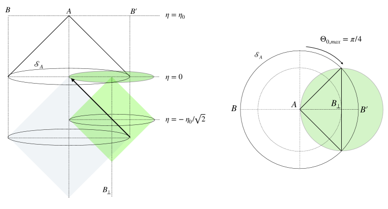
Figure 3: Causal relationships that define a maximal causal boundary (Eq. 14) on an antipodal cone. At left, a spacetime diagram with a history of causal relationships during inflation, as in the previous figures. An incoming axial trajectory is shown on ${\cal H}_{A}$ from the antipode $B^{\prime}$ of world line $B$. A causal diamond is shown centered at a position $B_{\perp}$ on this trajectory at the time $\eta=-\eta_{0}/\sqrt{2}$, whose boundary intersects ${\cal S}_{A}$ on a null plane orthogonal to the $AB^{\prime}$ axis. The right panel shows a slice through 3D space. Points on ${\cal S}_{A}$ at $\Theta>3\pi/4$ can receive information from events on the $AB^{\prime}$ axis of ${\cal H}_{A}$ prior to the end of inflation, so they can have causal correlations with displacements of $A$ along the $AB^{\prime}$ axis.

3.3.5 Maximal thin-sphere causal boundary

This boundary is not a shadow in the same sense as those just described, but represents a causal bound on possible exotic correlations in relation to an antipodal direction from coherent displacements of an emergent horizon footprint from its center, as shown in Fig. (3) and explained further below.

As shown in Fig. (3), the maximal boundary corresponds to the angle from an axis at which points on the axis are equidistant to the observed sphere and the observer,

$$\Theta_{0,\>\!\text{max}}=\pi/4.$$ (14)

A null plane that intersects a horizon footprint at this separation from an axis arrives at the observer at the same time as an orthogonal null plane. Within this angle, points on any footprint of ${\cal H}_{A}$ can receive information from events on the axial null trajectory on ${\cal H}_{A}$ prior to the end of inflation, so they can have a causal correlation with an axial displacement. The maximal boundary assumes independence of classical orthogonal directions relative to classical infinity, which is a more restrictive assumption than the causal-diamond overlap criterion adopted for causal shadows derived above.

3.3.6 Causal shadow at $\pi/2<\Theta<3\pi/4$

The relationships shown in Fig. (2) show boundaries of locations that share direct, classical two-way causal relationships with two world lines $A$ and $B$ during inflation. Causal correlations viewed by $A$ are confined to angular separations on a horizon footprint within a “shadow cone” that has an opening angle $\pi/2-\Theta_{0}$ with respect to the $B$ direction: that is, there is zero correlation at at all angular separations $\Theta>\pi/2-\Theta_{0}$. In particular, there is no causal connection of points on the horizon footprint surfaces at angles $\pi/2<\Theta<\pi$.

Because $A$ itself lies on ${\cal H}_{B}$, we should also allow for the possibility of “exotic” causal correlations at $\Theta>\pi/2$ from directional displacement of $A$ relative to its horizon, along the direction of the $AB$ axis. These correlations also have an angular causal boundary, now defined with respect to the antipodal point $B^{\prime}$. The angular boundary for causal connection with an axial displacement is given by the maximal causal boundary (Eq. 14), as shown in Fig. (3). At $\Theta>3\pi/4$, information from events on the $AB^{\prime}$ axis of $A$’s inflationary horizon can reach points on ${\cal S}_{A}$ before the end of inflation, so in principle it can produce a causal correlation of perturbations on ${\cal S}_{A}$ in the $AB^{\prime}$ antipodal cap.

In previous work (Hogan & Meyer, 2022; Hogan et al., 2023) we introduced models of this coherent antihemispheric correlation, based on time shifts by a classical gravitational null planar shock, where the analogous effect is a shift of the observer’s clock due to a shock displacement in a particular direction. Since the aim in the current study is to test the null symmetry without model-dependent assumptions, we adopt a conservative approach that avoids models of exotic antihemispheric correlations: we simply posit a causal shadow in relation to $\Theta=\pi$ with constraints like those in relation to $\Theta=0$. This constraint allows us to test for causal shadows with zero correlation in a range $\Theta<\pi/2+\Theta_{0,\>\!\text{max}}$ or $\Theta<\pi/2+\Theta_{0,\>\!2\text{D}}$, but does not exclude possible exotic nonzero correlation closer to the antipode.

3.3.7 Asymmetric causal shadow in total $C(\Theta)$

CMB anisotropy from SW and ISW effects arise at very different comoving distances, only some of which can create correlations at $\Theta>\pi/2$. For this reason, the causal shadow of total correlation including both effects is not symmetric around $\Theta=\pi/2$.

Late-time ISW is produced mainly by foreground structure at redshift $z\lesssim 1$, when the effect of dark energy modifies the background expansion significantly from that of a matter-dominated universe. Matter at these low redshifts is much closer than the radius of the smallest causal diamond entangled with the last scattering surface. Since the ISW effect from matter entangled with exotic displacement of that surface is negligible, ISW correlations essentially vanish for $\Theta>\pi/2-\arcsin(1/4)$.

As explained above, let us allow for the possibility of correlation at $\Theta>\pi/2$ from exotic antipodal thin-sphere SW anisotropy on the last scattering surface. The causal shadow in this case should conservatively extend to $\Theta=\pi/2+\Theta_{0,\>\!2\text{D}}=2\pi/3$, so the total shadow extends at least over the asymmetric range,

$$C([\pi/2-\arcsin(1/4)]<\Theta<2\pi/3)=0.$$ (15)

In principle the thin-sphere causal shadow could extend to the maximal boundary at

$$\Theta=\pi/2+\Theta_{0,\>\!\text{max}}=3\pi/4,$$

in which case the causal shadow of total correlation extends over a wider range,

$$C([\pi/2-\arcsin(1/4)]<\Theta<3\pi/4)=0.$$ (16)

We implement tests of both of these possibilities.

4 Causal Symmetry of CMB maps

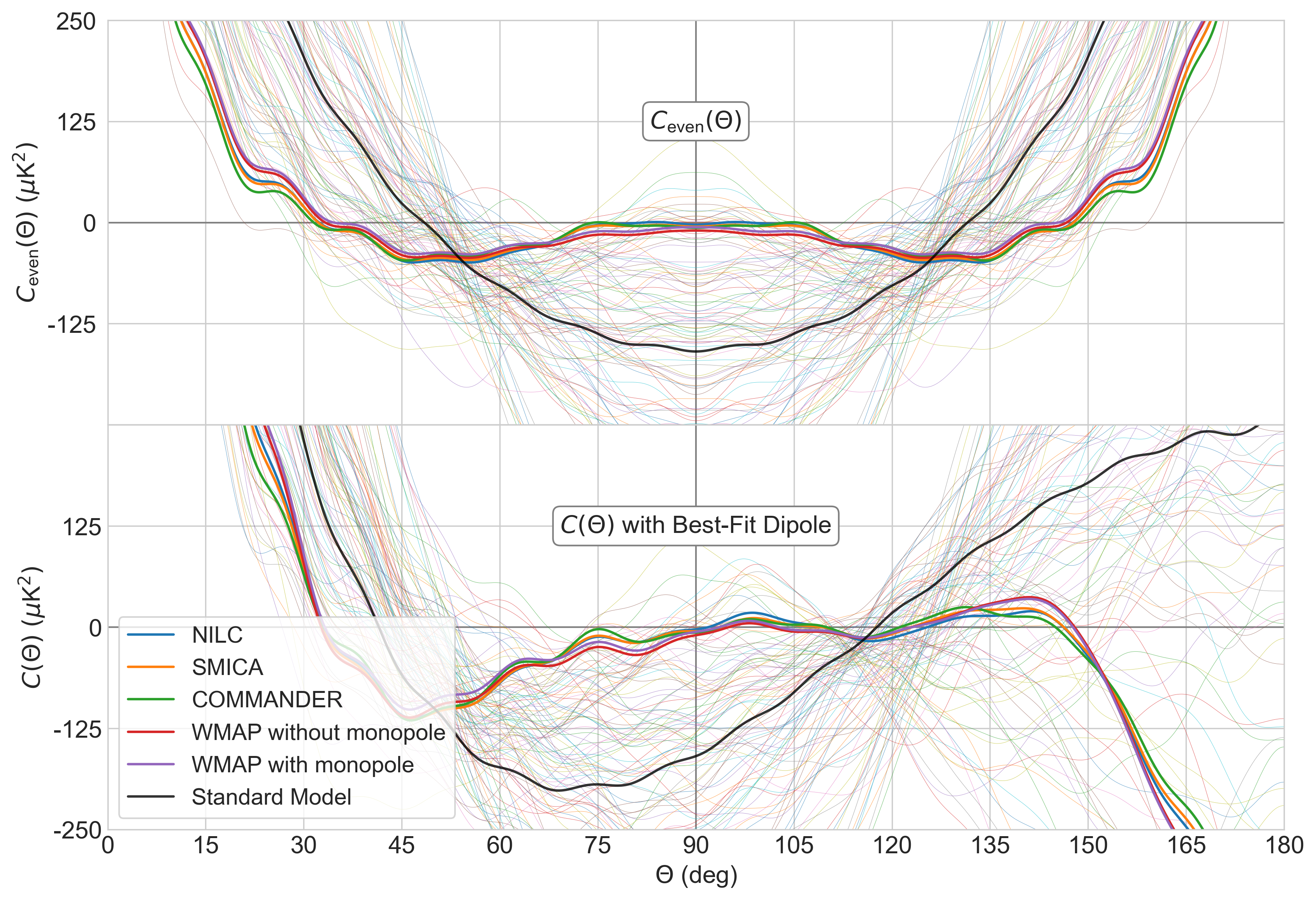
Figure 4: Correlation functions of sky maps and standard-model realizations. Bold colors show Galaxy-subtracted all-sky maps, as labeled. Solid black shows the expectation of the standard model. Fine lines show standard, randomly generated sky realizations. Top panel shows the even parity correlation with no corrections. Causal shadow symmetry predicts that this function should vanish over the band given by Eqs. (11) and (12), or $75.53^{\circ}<\Theta<104.47^{\circ}$, which is strikingly approximated by the maps, especially those from Planck data; for these, the residual correlation is about three orders of magnitude smaller than that in typical standard realizations, as shown quantitatively in Fig. (5). Bottom panel shows the total correlation with the best-fit dipole restored, assuming a causal shadow that extends over the maximum predicted range, $75.53^{\circ}<\Theta<135^{\circ}$ (Eq. 16). For a fair comparison, each realization has a “mock dipole” correction added to minimize its departure from zero in the shadow region. Again, the maps approximate zero more closely than almost any realization.

4.1 Dipole subtraction and parity separation

It is not possible to measure the true primordial pattern because the dipole components $a_{1m}$ have been removed from the maps to compensate for the local motion relative to the local cosmic rest frame. This motion is induced by perturbations, including our nonlinear orbits within the galaxy and the Local Group (Peebles, 2022).

Nevertheless, a small fraction of the subtracted dipole is part of the intrinsic large-angle primordial pattern on spherical causal diamond surfaces and contributes to correlation in the angular range of causal shadows. Thus, the whole shadow symmetry can only become apparent when the intrinsic portion of the dipole is included. Consequently, if the shadow symmetry is a true symmetry of the observed CMB temperature, then there must exist a dipole that can be added to the observed CMB temperature map that realizes the shadow symmetry.

The total correlation (Eq. 8) is a sum of even and odd Legendre polynomials, which are respectively symmetric and antisymmetric about $\Theta=\pi/2$. To produce zero correlation over a range symmetric around $\Theta=\pi/2$, no combination of even functions can cancel any combination of odd ones, so if an angular correlation function vanishes over a range $[\pi/2-\phi,\pi/2+\phi]$ symmetric about $\Theta=\pi/2$, the even contributions and the odd contributions to the angular correlation function must vanish independently over that range.

This property allows a direct, model- and dipole- independent test of causal symmetry, that uses only even-parity correlation. Over the angular range of a general 3D causal shadow (Eqs. 11 and 12), where total correlation vanishes in both hemispheres, the sum of even terms must vanish on its own, independently of any dipole or model parameters.

Furthermore, if the primordial angular correlation vanishes over an arbitrary range $[\alpha,\beta]$, then the sum of the even and odd Legendre polynomials for $\ell>1$ must be able to be cancelled over that range by an unknown dipole, a function of the form

$$\mathcal{D}(\Theta)=\frac{3}{4\pi}C_{1}\cos(\Theta),$$ (17)

where $C_{1}\geq 0$. Over the angular range of the total asymmetric shadow (Eq. 15 or 16), the sum of the even and odd Legendre polynomials for $\ell>1$ must vanish after addition of a dipole of unknown amplitude.

If the causal shadow symmetry is real, a perfect map of primordial anisotropy should satisfy both of these criteria. Our aim is to measure how closely the observed CMB data approximates these causal shadow predictions, and how its agreement compares with standard model realizations.

4.2 Data

As explained in Hagimoto et al. (2020), we use all-sky CMB maps made with subtracted models of Galactic emission, in order to minimize correlation artifacts introduced by masks. Our analysis is based on foreground-corrected maps of the CMB temperature based on the fifth and third public release databases of the WMAP and PLANCK collaborations, respectively. In the case of PLANCK, we use several different maps based on different techniques for modeling the Galaxy. Recognizing that the noise properties of the foreground-corrected maps are not well characterized and that the 2-point function is correlated between angles, we use the variation between foreground subtraction methods and experiments as a proxy for correlation function uncertainty. We only compare integrated residuals of measured values and standard model realizations of 2-point correlation functions.

For this paper, we used the python wrapper for the Hierarchical Equal Area isoLatitude Pixelization (HEALPix) scheme (Gorski et al., 2005) on maps at a resolution defined by $N_{\text{side}}=256$. We preprocessed the maps by converting them to this resolution and removing their respective dipole spherical harmonic moments. We conduct all measurements and operations on each map independently.

4.3 Correlations of maps and realizations

To generate standard model realizations, we used the Code for Anisotropies in the Microwave Background (CAMB) (Lewis & Challinor, 2011) to calculate $C_{\ell}^{\text{\,SM}}$ with the following six cosmological parameters from the Planck collaboration (Planck Collaboration, 2020b): dark matter density $\Omega_{c}h^{2}=0.120$; baryon density $\Omega_{b}h^{2}=0.0224$; Hubble constant $H_{0}=67.3$; reionization optical depth $\tau=0.054$; neutrino mass $m_{\nu}=0.06$ eV; and spatial curvature $\Omega_{k}=0.001$. For each realization, we calculated the angular power spectrum up to a cutoff of $\ell_{\text{max}}=30$ by Eq. 7. Then, we determined $C(\Theta)$ by summing Eq. 8 up to the sharp cutoff $\ell_{\text{max}}=30$. Correlation functions of realizations and CMB maps are shown in Fig. (4).

According to the causal shadow hypothesis, the even-parity correlation should vanish in the range of angles where all contributions to both odd and even contributions vanish (Eq. 11). As verified quantitatively by the rank comparison described below, the maps are indeed much closer to zero over this range than almost all realizations. Both the prediction and measurement in this comparison are model- and parameter-free, so the close agreement with zero in the expected range is striking.

Outside this range, where ISW anisotropy does not have even parity, the unmeasured dipole must be included to see the null symmetry, since odd- and even-parity harmonics must both be included to describe the total causal shadow. For a map with a causal shadow symmetry, an added cosine function (Eq. 17) reproduces the effect of restoring the unobserved intrinsic dipole.

Standard realized correlation functions include only $\ell>1$ harmonics. For the comparison shown in Fig. (4), each realization is modified with a function of the form in Eq. (17) to minimize its residuals from zero. For realizations, this term does not have any relation to an intrinsic physical dipole: it is a “mock dipole” added to estimate how frequently the sum of $\ell>1$ harmonics in Eq. (8) comes as close to the maps as those of a causal shadow model.

As is the case for the even parity correlation, it appears that the measured $C(\Theta)$ in the total shadow range (Eqs. 15 or 16) is closer to zero than almost all standard realizations, even when they have a mock dipole added.

4.4 Residuals

The striking visual impression of a null symmetry in the measured correlation can be verified quantitatively by a rank comparison of residuals.

Let $C_{\ell}$ denote the angular power spectrum of a measure CMB temperature map or a standard model realization. Then, we can define this power spectrum’s even-parity angular correlation function $C_{\text{even}}(\Theta)$ as

$$C_{\text{even}}(\Theta)=\frac{1}{4\pi}\sum_{\begin{subarray}{c}\ell\;\!=\;\!2,\;\!4,\;\!6,\;\!...\end{subarray}}^{\ell_{\text{max}}}(2\ell+1){C}_{\ell}P_{\ell}(\cos\Theta),$$ (18)

where $\ell_{\text{max}}=30$. Let $\{\Theta_{j,[\alpha,\beta]}\}_{i=1}^{N}$ denote a uniformly spaced lattice of points in the range $[\alpha,\beta]$. Then, define the residual

$$\Delta_{\text{even},[\alpha,\beta]}(C(\Theta)) \equiv\int_{\alpha}^{\beta}|C_{\text{even}}(\Theta)|^{2}\,d\Theta$$

$$\approx\sum_{i=1}^{N}[C_{\text{even}}(\Theta_{i,[\alpha,\beta]})]^{2}\cdot\left(\frac{\beta-\alpha}{N}\right)\!,\,$$ (19)

and the residual

$$\Delta_{\text{best-fit},[\alpha,\beta]}(C(\Theta)) \equiv\int_{\alpha}^{\beta}|\tilde{C}_{\beta}(\Theta)|^{2}\,d\Theta$$

$$\approx\sum_{i=1}^{N}[\tilde{C}_{\beta}(\Theta_{i,[\alpha,\beta]})]^{2}\cdot\left(\frac{\beta-\alpha}{N}\right)\!,\,$$ (20)

where

$$\tilde{C}_{\beta}=C+\mathcal{D}_{\text{best-fit}}$$

and $\mathcal{D}_{\text{best-fit}}$ is the dipole contribution that minimizes the residual. Next, let

$$\Delta_{\text{even}} \equiv\Delta_{\text{even},[\pi/2-\Theta_{0},\pi/2+\Theta_{0}]},$$ (21)

$$\Delta_{\text{general}} \equiv\Delta_{\text{best-fit},[\pi/2-\Theta_{0},2\pi/3]},$$ (22)

$$\Delta_{\text{maximal}} \equiv\Delta_{\text{best-fit},[\pi/2-\Theta_{0},3\pi/4]}.$$ (23)

We use these three residuals as a measure of how compatible a given power spectrum $\left\{C_{\ell}\right\}_{\ell>1}$ is with the causal shadow symmetry. Each of the integrals must vanish for such a power spectrum that exactly agrees with the causal shadow symmetry. In practice, we found that $N=2000$ is a sufficiently high lattice resolution to approximate the integrals among different data sets and standard model realizations with negligible error.

Figure 5: Cumulative probability of deviations from zero correlation in standard realizations, compared with deviations of CMB maps, within computed causal shadow angular ranges. The top panel directly compares model- and dipole-independent deviations of even-parity correlation over the general 3D causal shadow (Eqs. 11 and 12). No parameters are used for this comparison. The middle panel compares deviations of total correlation over the general asymmetric shadow (Eq. 15), and the bottom panel compares deviations of total correlation over the general asymmetric shadow (Eq. 16); both of these allow for a mock-dipole correction to minimize residuals for each realization. In spite of variation between the maps, they are all much closer to zero than almost all standard realizations. The measured departures from zero do not significantly exceed the differences between the maps, as expected if they are dominated by systematic measurement errors. In all of these comparisons, the Planck maps match the symmetry better than the WMAP maps: in the cleanest direct comparison represented by the top panel, the measured residuals of all the Planck maps are less than $10\mu{\rm K}^{2}$, about three orders of magnitude smaller than those of typical realizations, with cumulative probabilities from $10^{-4.3}$ to $10^{-2.8}$.

4.5 Rank comparison of shadow symmetry with standard realizations

Our three tests are as follows. First, we generate $N=2\cdot 10^{6}$ standard model realizations. We then evaluate $\Delta_{\text{even}}(C(\Theta))$, $\Delta_{\text{general}}(C(\Theta))$, and $\Delta_{\text{maximal}}(C(\Theta))$ for these standard model realizations, such as those shown in Fig. (4), as well as the different measured CMB maps. For a given residual $\Delta_{\text{even}}$, $\Delta_{\text{general}}$, or $\Delta_{\text{maximal}}$, the variance between the values of this residual for different measured CMB maps gives a measure of the sensitivity of the residual to Galactic model uncertainties.

The top panel of Fig. (5) shows cumulative probability, the fraction of standard realizations with $\Delta_{\text{even}}$ smaller than the value shown on the horizontal axis, and the vertical lines show the values of $\Delta_{\text{even}}$ for different measured CMB maps. We find that a small fraction of standard model realizations, ranging from $10^{-1.5}$ (for WMAP) to $10^{-4.3}$ (for NILC), come as close to zero $\Delta_{\text{even}}$ as the measured CMB temperature maps.

The middle panel shows the same quantities evaluated for $\Delta_{\text{general}}$, with the dipole-term adjustment described above. We again find that a small fraction of standard model realizations, ranging from about $10^{-1.8}$ (for WMAP) to $10^{-2.8}$ (for Commander), come as close to zero $\Delta_{\text{general}}$ as the measured CMB temperature maps. The values of $C_{1}$ for the best-fit dipole for the maps NILC, SMICA, COMMANDER, WMAP without its monopole, and WMAP with its monopole are approximately $365$, $341$, $322$, $392$, and $426$ $\mu$K², respectively.

The lower panel shows the same quantities evaluated for $\Delta_{\text{maximal}}$, with the dipole-term adjustment described above. We again find that a small fraction of standard model realizations, ranging from about $10^{-2.3}$ (for WMAP) to $10^{-3.2}$ (for Commander), come as close to zero $\Delta_{\text{maximal}}$ as the measured CMB temperature maps. The values of $C_{1}$ for the best-fit dipole for the maps NILC, SMICA, COMMANDER, WMAP without its monopole, and WMAP with its monopole are approximately $384$, $390$, $389$, $440$, and $471$ $\mu$K², respectively.

To evaluate the sensitivity of this test to the chosen cutoff $\ell_{\text{max}}$, we repeated the aforementioned tests for every $\ell_{\text{max}}$ value ranging from $25$ to $35$. The significance of our results, i.e. the fraction of standard model realizations having $\Delta_{\text{even}}$ as low as the measured CMB temperature maps, changed by less than $2\cdot 10^{-3}$; the fraction of standard model realizations having $\Delta_{\text{general}}$ as low as the measured CMB temperature maps changed by less than $3\cdot 10^{-4}$; and fraction of standard model realizations having $\Delta_{\text{maximal}}$ as low as the measured CMB temperature maps changed by less than $2\cdot 10^{-4}$.

5 Interpretation

As seen in Fig. (4), correlations measured within calculated causal shadow boundaries appear to be consistent with zero true correlation, in the sense that deviations from zero are comparable with differences between the data from different foreground-subtracted maps. The symmetry is particularly striking in the direct measurement of even-parity correlation over the range of angles where it is expected to vanish. The data are also consistent with nearly-zero total correlation over the calculated range for the total shadow, after allowing for an unobserved dipole.

The standard interpretation is that the tiny correlation of the real sky represents a statistical anomaly, but this occurs in a only small fraction of realizations. A rank comparison (Fig. 5) shows that the sky agrees with zero better than almost all standard realizations. The most significant effect appears in the even-parity symmetry: Planck maps show deviations from zero several orders of magnitude smaller than typical standard realizations, which happens in only a fraction $10^{-2.8}$ to $10^{-4.3}$ of realizations, depending on the map.

Our proposed interpretation is that the small correlation is due to a fundamental causal symmetry of quantum gravity. It results directly from the basic physical principle of causal coherence: quantum fluctuations only generate physical correlations in regions bounded by causal diamonds. In this interpretation, the small measured departure from zero correlation is attributed to measurement error dominated by contamination by the Galaxy. This view is consistent with measured variation among the different maps.

6 Conclusion

The surprisingly small absolute value of the large-angle CMB correlation function has been known since the first measurements with COBE (Bennett et al., 1994; Hinshaw et al., 1996). Better measurements from WMAP (Bennett et al., 2003, 2011) and then Planck (Planck Collaboration, 2020c) show values successively closer to zero. This anomaly and others have been thoroughly analyzed (e.g., Copi et al. (2009), Muir et al. (2018), Jones et al. (2023)), but are not generally thought to present a compelling challenge to standard cosmological theory, partly because there has not been a precisely formulated and physically motivated alternative expectation.

As shown here, the anomalously small correlation becomes even more striking if the possibility of an intrinsic, unobserved dipole component is accounted for. Direct measurements of even-parity correlation, and of total correlation after allowing for an intrinsic dipole, both reveal an amplitude for the 2-point function that is significantly smaller than generally appreciated. Indeed, the maps appear to be consistent with zero correlation over a specific range of angular separation that coincides with that expected from an absence of correlations between timelike intervals on world lines without a shared causal history, determined by overlap of causal diamonds during inflation.

We account for this apparent symmetry with a new physical hypothesis. Our direct geometrical reasoning explains how a causal correlation shadow like that observed can emerge from standard, covariant, two-way causal relationships, and precisely specifies its angular boundaries. Unlike some other candidate explanations for large-angle CMB anomalies, it is based only on well established principles that govern causal physical relationships. Our analysis takes account of all significant gravitational contributions of primordial perturbations to large-angle CMB correlation, including ISW.

We thus interpret the causal shadow not as an anomaly, but as an exact symmetry of quantum vacuum fluctuation states that are coherent on causal diamonds. This quantum “spookiness” of gravitational fluctuations is not consistent with the standard model of inflationary perturbations based on quantum field theory, but would be required for a theory of quantum gravity to address long-wavelength causal inconsistencies with QFT.

Our interpretation is consistent with current tests of classical concordance cosmology, which depend only on a nearly scale-invariant initial 3D power spectrum of perturbations, and with applications of QFT that do not involve quantized gravity. More tests are possible of the two-point correlation shadows studied here, as well as other causal CMB signatures, and these will improve with all-sky maps of the Galaxy that allow better measurements of the true CMB pattern on the largest scales. Universal causal constraints on correlations can be further tested with maps of late-time large-scale structure, especially with surveys of large-scale linear structure that can reveal whether inflationary perturbations around other locations reveal the same exotic causal constraints as the CMB. Some of these tests are discussed briefly in the Appendix.

Standard inflation theory assumes, in spite of long known theoretical difficulties, that QFT describes the behavior of physical quantum gravity on large scales. Our analysis reveals signatures of a real-world symmetry that contradicts this assumption, but conforms with coherent quantum geometrical fluctuations expected in a deeper, causally consistent fundamental theory. It appears that large-scale correlations of CMB anisotropy may provide direct, unique and specific evidence for a deeper theory.

7 Appendix

7.1 Implications of causal coherence for standard cosmology

A causal symmetry of primordial perturbations requires a causal spacetime constraint on quantum coherent states that is inconsistent with the standard QFT model used to compute classical perturbations that form from quantum vacuum fluctuations.

At a basic level, a causal shadow is incompatible with standard cosmic variance, which predicts vanishing angular correlation only for a set of angular separations of measure zero. In the standard QFT quantum model, orthogonal modes are assumed from the outset to commute; hence, the model of horizons and mode freezing for each axis is a separable one dimensional system, which leads to the standard cosmic variance for realized classical angular correlation. Causal shadows over a finite range of angles can only appear if there is gravitational entanglement with causal structure, so that orthogonal components of fluctuating position and momentum do not commute for quantum states on the scale of whole causal diamonds.

As noted previously, such holistic behavior may be needed in any case to address the IR problems of QFT (Cohen et al., 1999; Hollands & Wald, 2004; Stamp, 2015), and can be accommodated in principle by “holographic” theories of gravity (Jacobson, 1995, 2016; Bousso, 2002; Banks, 2023a, b). Causal coherence has previously been invoked to motivate direct laboratory searches for quantum fluctuations of causal structure (Chou et al., 2017; Richardson et al., 2021; Vermeulen et al., 2021).

Although causal coherence of gravitational fluctuations is not possible in QFT, it is consistent with the myriad predictions of QFT that do not include gravitational quantum interactions: cosmological perturbations are the only currently measured phenomenon that depends on active quantum gravity. A causal shadow in the CMB would be a unique direct signature of quantum gravity that conflicts with QFT, and as such, would provide a specific empirical constraint on holographic quantum theories of gravity.

Since coherence of fluctuations in causal diamonds requires a fundamentally different quantum model for the formation of perturbations, it alters aspects of cosmological theory that depend in detail on the internal dynamics of the QFT model (Hogan, 2019, 2020). For example, causally-coherent gravitational fluctuations are much larger than QFT fluctuations for a given inflationary expansion rate $H$; the variance of curvature on the horizon scales like $\Delta^{2}\simeq H$ in Planck units, as opposed to $\Delta^{2}\simeq H^{2}$ in the QFT picture. Thus, estimated parameters for the effective inflaton potential based on fluctuation amplitude and tilt need to be modified in a causally-coherent theory.

In spite of these fundamental theoretical differences, causal coherence does not alter predictions based on classical relativity. In the context of late-time concordance $\Lambda$CDM cosmology, the main observable constraints on standard inflation depend only on a direction-averaged 3D power spectrum of relict curvature perturbations. In standard theory, QFT produces inflationary perturbations with the required nearly-scale-invariant power spectrum, given an effective inflaton potential with a suitably tuned amplitude and slope. The same spectrum would also be produced in a holographic model with a smaller, and suitably slowly-changing inflationary expansion rate.

If causal shadows result from causal coherence of quantum geometry, that coherence extends without bound to horizons of any macroscopic scale. The reduction of a quantum state to the specific observed classical pattern of perturbations is an ongoing process that unfolds after inflation on larger scales, encompassing and revealing causal diamonds that begin earlier during inflation. The existence of causal shadows thus fits naturally into a quantum cosmology that includes entanglement with states of a “participatory observer,” even on the largest scales (Wheeler, 1989).

7.2 Statistical isotropy and locality

Formulations of cosmological theories often begin with posited a priori symmetries of the whole cosmological system, such as a “Cosmological Principle” that nature does not define a preferred location or direction, or the Galilean principle that all observers are equivalent. The mathematical implementation of these ideas in a quantum theory depends on how quantum nonlocality and “spookiness” are implemented in quantum gravity.

The standard formulation is based on the symmetry of the classical homogeneous and isotropic FLRW cosmological solutions as a background. With a Fourier transform, the unbounded 3D space permits a unique equivalent description in comoving $\vec{k}$ space. This setup leads to a quantum system that creates a “statistically isotropic” global ensemble of spatially infinite perturbations, and an ensemble of realizations with standard cosmic variance. In any particular realization of the ensemble, a finite part of the system is manifestly not isotropic, since a horizon of any size is distorted by anisotropic perturbations from a still larger scale.

By contrast, a causally-coherent, relational theory does not assume a preexisting 3+1D cosmological background. The system still adopts the basic principle that neither the laws of physics nor the universe as whole define a preferred direction or location in spacetime, but in a cosmological (as in any) realization of a quantum system, any observer is of necessity (and equivalently) privileged. There is no preordained infinite physical background spacetime; instead, inflation generates a large but finite system that approximates a classical FLRW solution with emergent standard causal relationships.

7.3 Further tests of primordial causal coherence

7.3.1 CMB maps with better Galaxy models

The causal shadow prediction is unambiguous, and falsifiable in principle. The cleanest way to disprove it would be to show that there is nonzero primordial correlation in the shadow. Conversely, the most convincing empirical reason to doubt the QFT model comes from the large likelihood contrast between the symmetry and the standard model realizations, which already exceeds $10^{4}$ for some maps.

Both of these comparisons are currently limited by uncertainties in Galactic foregrounds. For a convincing test, it is necessary to show that a causal shadow either is or is not present in the CMB pattern itself to a high degree of precision.

In the analysis presented above, we have used the published all-sky, unmasked, Galaxy-subtracted CMB maps prepared by the satellite teams. We have not undertaken a close comparative study of the Galaxy models used to create those maps, but it is plausible that existing data from WMAP and Planck could be used to create new maps optimized for the purpose of testing a null correlation hypothesis over a specific range of angular separation. A definitive test may require better spectral measurements than current maps, as proposed in new satellite concepts such as LiteBird and PIXIE.

7.3.2 Exotic correlations in 3D large scale structure

Universal causal constraints apply to the angular distribution of primordial perturbations around any point. Linear evolution of density perturbations on the largest scales approximately preserves the primordial pattern at large angular separation, in relation to any comoving location. Even on scales where the primordial pattern is modified by baryon acoustic oscillations before recombination, the dark matter dominates the overall density and gravitational potential by significant factor. Thus, residual effects of causal constraints should appear in subvolumes of large, complete spectroscopic surveys, such as BOSS, DESI, and Euclid (Hogan, 2019). Their signatures should appear in higher-order correlations in three dimensions.

A particularly distinctive signature of causal coherence should appear as global parity violation. CMB correlations at the largest separations appear to have a negative correlation function,

$$C(\Theta\rightarrow\pi)<0,$$ (24)

which corresponds to an excess of odd over even spectral perturbation power at large angular separation. This significant excess of net odd parity power is detected even at higher resolution, at least to $\ell\simeq 30$ (Planck Collaboration, 2016). This parity violation, if it is attributed to a universal property of holographic quantum gravitational fluctuations, should affect perturbations on all linear scales. They are not erased by baryonic oscillations, which change phase but not parity. An exotic origin of parity violation may account for recent detections of parity violation in the large-scale galaxy distribution (Hou et al., 2022; Philcox, 2022) that are difficult to account for in the standard scenario of a QFT-based $\mathbb{P}$-symmetry violation (Philcox, 2023).

7.4 Other causal signatures in the CMB pattern

We have shown how causal boundaries of coherent gravitational fluctuations, in the form of axially symmetric circular intersections of spherical causal diamond boundaries on the sky, can be preserved in universal statistical properties of the CMB pattern. In general, the same geometrical relationships from causal coherence should lead to other identifiable statistical signatures that go beyond the correlation shadows of $C(\Theta)$ considered above.

For example, a causal diamond is not entangled with horizons of world lines centered farther away than twice its horizon footprint radius, as shown by the detachment of ${\cal S}_{AB/2}$ from horizons of world lines more distant than $B$ in Fig. (2). Thus, footprints should have universal, orientation-independent angular power spectra in equatorial stripes bounded by circles with the opening angles of the 3D causal shadow (Eqs. 11, 12)— a more general constraint than the correlation zero in the same range.

The complementary causal boundary of entanglement with smaller causal diamonds, also seen in Fig. (2), is the maximum angular separation of world lines on a spherical horizon footprint ${\cal S}_{B}$ that have a two-way causal connection after leaving the horizon ${\cal H}_{B}$, but before the end of inflation. Points on ${\cal S}_{B}$ are disentangled in this sense if they are separated by more than half the radius of ${\cal S}_{B}$, or

$$\Theta_{AB/2}=2\arcsin(1/4)\simeq 28.96^{\circ}.$$ (25)

Correlations with any direction at smaller angular separation than $\Theta_{AB/2}$ are independent of those at larger separation, so their local behavior approximates the standard QFT picture. If disentanglement produces independent even- and odd-parity correlations in circular patches of radius $\Theta_{AB/2}$ around any point and its antipode, there should be zeros in $C(\Theta)$ at $\Theta_{AB/2}$ and $\pi/2-\Theta_{AB/2}$ in dipole-free maps. It is noteworthy that zeros of CMB correlation are indeed measured at $\Theta\simeq 30^{\circ}$ and $\Theta\simeq 150^{\circ}$ in unmasked CMB maps (Hagimoto et al., 2020).

These and other exotic causal signatures can be differentiated from generic QFT realizations, and from generic anomalies, by specific, precisely calculable and measurable causal boundaries in the angular domain. They are most conspicuous at angular separations much larger than in previous studies of $N>2$-point functions designed mainly as probes of primordial nongaussianity in the QFT framework.

References

- Banks (2023a) Banks, T. 2023a, arXiv e-prints, arXiv:2306.07038, doi: 10.48550/arXiv.2306.07038
- Banks (2023b) —. 2023b, arXiv e-prints, arXiv:2309.07203, doi: 10.48550/arXiv.2309.07203
- Bardeen (1980) Bardeen, J. M. 1980, Phys. Rev. D, 22, 1882, doi: 10.1103/PhysRevD.22.1882
- Baumann (2011) Baumann, D. 2011, in Physics of the large and the small, TASI 09, 523–686, doi: 10.1142/9789814327183_0010
- Bennett et al. (1994) Bennett, C. L., Kogut, A., Hinshaw, G., et al. 1994, ApJ, 436, 423, doi: 10.1086/174918
- Bennett et al. (2003) Bennett, C. L., Halpern, M., Hinshaw, G., et al. 2003, The Astrophysical Journal Supplement Series, 148, 1, doi: 10.1086/377253
- Bennett et al. (2011) Bennett, C. L., Hill, R. S., Hinshaw, G., et al. 2011, The Astrophysical Journal Supplement Series, 192, 17. http://stacks.iop.org/0067-0049/192/i=2/a=17
- Bousso (2002) Bousso, R. 2002, Rev.Mod.Phys., 74, 825, doi: 10.1103/RevModPhys.74.825
- Chou et al. (2017) Chou, A., Glass, H., Gustafson, H. R., et al. 2017, Class. Quant. Grav., 34, 165005, doi: 10.1088/1361-6382/aa7bd3
- Cohen et al. (1999) Cohen, A. G., Kaplan, D. B., & Nelson, A. E. 1999, Phys. Rev. Lett., 82, 4971
- Copi et al. (2009) Copi, C. J., Huterer, D., Schwarz, D. J., & Starkman, G. D. 2009, Mon. Not. Roy. Astron. Soc., 399, 295, doi: 10.1111/j.1365-2966.2009.15270.x
- Francis & Peacock (2010) Francis, C. L., & Peacock, J. A. 2010, Monthly Notices of the Royal Astronomical Society, 406, 14, doi: 10.1111/j.1365-2966.2010.16866.x
- Gorski et al. (2005) Gorski, K. M., Hivon, E., Banday, A. J., et al. 2005, The Astrophysical Journal, 622, 759, doi: 10.1086/427976
- Hagimoto et al. (2020) Hagimoto, R., Hogan, C., Lewin, C., & Meyer, S. S. 2020, The Astrophysical Journal, 888, L29, doi: 10.3847/2041-8213/ab62a0
- Hinshaw et al. (1996) Hinshaw, G., Banday, A. J., Bennett, C. L., et al. 1996, The Astrophysical Journal, 464, L25, doi: 10.1086/310076
- Hogan (2019) Hogan, C. 2019, Phys. Rev. D, 99, 063531, doi: 10.1103/PhysRevD.99.063531
- Hogan (2020) —. 2020, Classical and Quantum Gravity, 37, 095005, doi: 10.1088/1361-6382/ab7964
- Hogan & Meyer (2022) Hogan, C., & Meyer, S. S. 2022, Classical and Quantum Gravity, 39, 055004, doi: 10.1088/1361-6382/ac4829
- Hogan et al. (2023) Hogan, C., Meyer, S. S., Selub, N., & Wehlen, F. 2023, Classical and Quantum Gravity, 40, 165012, doi: 10.1088/1361-6382/ace608
- Hollands & Wald (2004) Hollands, S., & Wald, R. M. 2004, General Relativity and Gravitation, 36, 2595, doi: 10.1023/b:gerg.0000048980.00020.9a
- Hou et al. (2022) Hou, J., Slepian, Z., & Cahn, R. N. 2022. https://arxiv.org/abs/2206.03625
- Hu & Dodelson (2002) Hu, W., & Dodelson, S. 2002, Ann. Rev. Astron. Astrophys., 40, 171, doi: 10.1146/annurev.astro.40.060401.093926
- Jacobson (1995) Jacobson, T. 1995, Phys. Rev. Lett., 75, 1260
- Jacobson (2016) —. 2016, Phys. Rev. Lett., 116, 201101, doi: 10.1103/PhysRevLett.116.201101
- Jones et al. (2023) Jones, J., Copi, C. J., Starkman, G. D., & Akrami, Y. 2023. https://arxiv.org/abs/2310.12859
- Lewis & Challinor (2011) Lewis, A., & Challinor, A. 2011, CAMB: Code for Anisotropies in the Microwave Background, Astrophysics Source Code Library, record ascl:1102.026. http://ascl.net/1102.026
- Mackewicz & Hogan (2022) Mackewicz, K., & Hogan, C. 2022, Classical and Quantum Gravity, 39, 075015, doi: 10.1088/1361-6382/ac5377
- Muir et al. (2018) Muir, J., Adhikari, S., & Huterer, D. 2018, Phys. Rev. D, 98, 023521, doi: 10.1103/PhysRevD.98.023521
- Peebles (2022) Peebles, P. J. E. 2022, Anomalies in Physical Cosmology. https://arxiv.org/abs/2208.05018
- Philcox (2022) Philcox, O. H. E. 2022, Phys. Rev. D, 106, 063501, doi: 10.1103/PhysRevD.106.063501
- Philcox (2023) —. 2023. https://arxiv.org/abs/2303.12106
- Planck Collaboration (2016) Planck Collaboration. 2016, Astron. Astrophys., 594, A16, doi: 10.1051/0004-6361/201526681
- Planck Collaboration (2020a) —. 2020a, Astron. Astrophys., 641, A7, doi: 10.1051/0004-6361/201935201
- Planck Collaboration (2020b) —. 2020b, Astron. Astrophys., 641, A6, doi: 10.1051/0004-6361/201833910
- Planck Collaboration (2020c) —. 2020c, Astron. Astrophys., 641, A7, doi: https://doi.org/10.1051/0004-6361/201935201
- Richardson et al. (2021) Richardson, J. W., Kwon, O., Gustafson, H. R., et al. 2021, Phys. Rev. Lett., 126, 241301, doi: 10.1103/PhysRevLett.126.241301
- Sachs & Wolfe (1967) Sachs, R. K., & Wolfe, A. M. 1967, ApJ, 147, 73, doi: 10.1086/148982
- Stamp (2015) Stamp, P. C. E. 2015, New Journal of Physics, 17, 065017, doi: 10.1088/1367-2630/17/6/065017
- Vermeulen et al. (2021) Vermeulen, S., Aiello, L., Ejlli, A., et al. 2021, Classical and Quantum Gravity, 38, 085008, doi: 10.1088/1361-6382/abe757
- Wheeler (1989) Wheeler, J. A. 1989, in Proc. III Int. Symp. Foundations of Quantum Mechanics, ed. S. Kobayashi (Tokyo, Japan: Physical Society of Japan), 309–336. https://philpapers.org/archive/WHEIPQ.pdf
- Zeilinger (1999) Zeilinger, A. 1999, Rev. Mod. Phys., 71, S288, doi: 10.1103/RevModPhys.71.S288