On the Trajectories of SGD Without Replacement

Abstract

This article examines the implicit regularization effect of Stochastic Gradient Descent (SGD). We consider the case of SGD without replacement, the variant typically used to optimize large-scale neural networks. We analyze this algorithm in a more realistic regime than typically considered in theoretical works on SGD, as, e.g., we allow the product of the learning rate and Hessian to be $O(1)$.

Our core theoretical result is that optimizing with SGD without replacement is locally equivalent to making an additional step on a novel regularizer. This implies that the trajectory of SGD without replacement diverges from both noise-injected GD and SGD with replacement (in which batches are sampled i.i.d.). Indeed, the two SGDs travel flat regions of the loss landscape in distinct directions and at different speeds. In expectation, SGD without replacement may escape saddles significantly faster and present a smaller variance.

Moreover, we find that SGD implicitly regularizes the trace of the noise covariance in the eigendirections of small and negative Hessian eigenvalues. This coincides with penalizing a weighted trace of the Fisher Matrix and the Hessian on several vision tasks, thus encouraging sparsity in the spectrum of the Hessian of the loss in line with empirical observations from prior work. We also propose an explanation for why SGD does not train at the edge of stability (as opposed to GD).

1 Introduction

1.1 The Problem and the Background

This article examines the implicit regularization effect of Stochastic Gradient Descent (SGD) without replacement, also known as random reshuffling. This is the particular variant of SGD most commonly used in practice to optimize large-scale neural networks.

To put this into context, recall that gradient descent (GD) and its variants are a generic set of algorithms for minimizing an empirical loss $L$, which depends on a set of parameters $\theta$ and a dataset $D$ of size $n$. Specifically, the update to the parameters $\theta_{i}$ after the first $i$ steps of optimization is as follows:

$$\theta_{i+1}\quad=\quad\theta_{i}\ \ -\ \ \frac{\eta}{b}\sum_{z\in B_{i+1}}\nabla_{\theta}L(\theta_{i},z),\qquad i=0,1,\ldots,$$

where the $i$-th batch $B_{i}$ is a subset of the training dataset $D$ of size $b$ and $\eta$ is the step size (or learning rate). Full-batch gradient descent corresponds to the case when $B_{i}=D$ is the entire dataset, whereas mini-batch SGD corresponds to smaller values of $b$. In practice, smaller values of $b$ are both computationally faster and often lead to better performance [Bottou, 2009, Bottou, 2012, LeCun et al., 2012, Bengio, 2012]. The gain in speed is almost immediate since loss gradients at each step must only be computed on the current batch (see §2.1). The nature of the improvement in model quality from smaller values of $b$, however, is less obvious.

Variants of SGDs on Toy Shallow Networks
\begin{overpic}[width=433.62pt,height=563.7073pt]{images/gradient_descent_plot_ab_addittive.png} \put(1.0,90.0){\hbox{\pagecolor{white}GD with Gaussian noise}} \end{overpic} \begin{overpic}[width=433.62pt,height=563.7073pt]{images/gradient_descent_plot_ab_sgd_with_400.png} \put(15.0,90.0){\hbox{\pagecolor{white}SGD with repl.}} \end{overpic} \begin{overpic}[width=433.62pt,height=563.7073pt]{images/gradient_descent_plot_ab_sgd_400.png} \put(8.0,90.0){\hbox{\pagecolor{white}SGD without repl.}} \end{overpic}

Figure 1: Here are the dynamics in the setting outlined in §B, for small (red) and big (orange) learning rates. The colored surface is the loss landscape, the blue line is the manifold of minima, the white bullet is the initialization, and the magenta bullets are the lowest norm solutions. SGD without and with replacement both move towards the lowest norm solution, unlike noised GD. However, SGD without replacement is converging faster, with better accuracy, while steadily reducing the variance. SGD with replacement is approaching slower and will oscillate around it with a higher variance and less precision.

The differences between full-batch GD and mini-batch SGD have been extensively studied both empirically, e.g., [Keskar et al., 2016, He et al., 2019, Jastrzębski et al., 2021] and theoretically, e.g., [Kleinberg et al., 2018, HaoChen et al., 2020, Damian et al., 2021, Li et al., 2022, Chen et al., 2023]. However, virtually all the well-known theoretical work, except [Gürbüzbalaban et al., 2021, Mishchenko et al., 2020, Roberts, 2021, Smith et al., 2021], treats only the case of mini-batch SGD with replacement, in which the batches $B_{i}$ are sampled i.i.d. The goal of this article, in contrast, is to give a theoretical analysis of a significantly more realistic setting for mini-batch SGD in which we consider:

• The algorithm practitioners use: We analyze the algorithm most commonly used in practice to optimize large-scale neural networks, called SGD without replacement or sometimes random reshuffling, see §2.1. The key difference between SGD with and without replacement is that batches sampled without replacement are disjoint and form a random partition of the training dataset. These batches are, therefore, statistically dependent. This induces empirical differences, see, e.g., Fig. 1, and mathematical challenges, see §2.3. We also prove that it leads to qualitatively different behaviors than SGD with replacement, see §1.3 and §8.

• In real-world optimization regimes: Previous analyses of SGD made strong assumptions on the step size $\eta$, the number $k$ of steps of SGD that are analyzed (usually one epoch at time), or the size of the derivatives of the loss $L$. For instance [Smith et al., 2021] asks that

  $$\eta\ \cdot\ k\ \cdot\ \|\nabla L\|\quad\ll\quad 1\qquad\quad\text{and}\quad\qquad\eta\ \cdot\ k\ \cdot\ \|\nabla^{2}L\|\quad\ll\quad 1.$$ (1)

  The first hypothesis roughly requires that the total movement in parameter space is small and corresponds to allowing a local analysis for SGD. We will keep this assumption in the present work. However, we drop the second, see §J, that is often unrealistic, as we explain in §2.4. For instance, a well-known empirical observation about neural networks – known as progressive sharpening [Jastrzębski et al., 2019, Cohen et al., 2021, Cohen et al., 2022, Damian et al., 2023] – is that $\left\|\nabla^{2}L\right\|$ often grows throughout training until it is of order $\eta^{-1}$.

1.2 Informal Overview of the Results

We provide here an overview of our results with an emphasis on new insights into the differences between SGD with and without replacement. We also offer several theoretical insights that can help explain a range of phenomena empirically observed in training large neural networks. Our analysis is very general and does not make any assumptions about the learning task, model, or data set.

We start with an informal statement of our main result. We show that, relative to full-batch GD, SGD without replacement implicitly adds a regularizer. This penalizes the covariance of the gradients or analogously the norm of the loss gradients, measured in a loss-dependent norm determined by the Hessian of the loss.

Theorem 1 (Informal corollary of Theorem 2).

In expectation over batch sampling, one epoch of SGD without replacement differs from the same number of steps of SGD with replacement or GD, by an additional step on a regularizer. At a stationary point, the step on the $i-th$ parameter is

$$\begin{split}step_{i}\quad=\quad-\frac{\eta}{b-1}\ \sum_{\text{params }j}R_{i,j}\ \cdot\ \frac{d}{d\theta_{i}}\operatorname{Cov}_{z\in D}\big{(}\nabla L(\theta,z)\big{)}_{j,j}\end{split}$$

Where $R$ is a function of the Hessian. Away from a stationary point, there is an additional term dependent on the trace of the empirical covariance of the Hessian.

Note that, in expectation, the trajectories of GD and SGD with replacement are the same. However, Theorem 1 indicates that SGD without replacement is different, even on average. We also discuss how SGD with and without replacement have different variances, see §A.

Our goal in the rest of this section is to describe the nature of the regularizer from Theorem 1 and, in particular, the role of $R$ in driving qualitatively different behaviors between SGD with and without replacement. As a starting point, let us consider a stationary point $\theta$ for the full-batch loss $L(\theta,D)$. The matrix $R$ depends on $\theta$ and is a function of the Hessian of the loss $\nabla^{2}L$ and its variance. The bias of Theorem 1 corresponds to a sum of steps with learning rate $\eta/b$ and a power of the Hessian as preconditioning matrix on some regularizers, all of the following form

$$trace\big{(}S\cdot\operatorname{Cov}_{z\in D}\big{(}\nabla L(\theta,z)\big{)}\big{)}\quad=\quad\mathbb{E}_{z\in D}\big{[}\|\nabla L(\theta,z)-\nabla L(\theta,D)\|_{S}^{2}\big{]}$$ (2)

for some matrix $S$ that is a function of the Hessian and inherits its eigenspaces. Let us work on a basis of eigenvectors $\{\theta_{1},\theta_{2},\ldots\}$ for the Hessian corresponding to the eigenvalues $\{\lambda_{1},\lambda_{2},\ldots\}$ and define the effective step size $c=\eta k>0$. Then we have that the entries of $R_{i,j}$ are

$$R_{i,j}\quad=\quad\frac{1}{2}\sum_{h=0}^{k+2}(-\eta\lambda_{i})^{h}\sum_{l=h+2}^{k}\binom{k}{l}(-\eta\lambda_{j})^{l-h-2}$$

and they approximately correspond to the following quantities

$$R_{i,j}\quad\sim\quad\frac{c}{2}\cdot\begin{cases}\frac{1}{2}\!\!\qquad\qquad\qquad\qquad\qquad\quad\text{ constant}\qquad&\text{ if }c\lambda_{i},c\lambda_{j}\text{ small}\\ (c\lambda_{i})^{-1}\hskip 1.13791pt\quad\qquad\qquad\quad\qquad\text{ small}&\text{ if }c\lambda_{i}\gg 0,c\lambda_{j}\text{ small}\\ (c\lambda_{j})^{-1}\quad\qquad\qquad\qquad\quad\text{ small}&\text{ if }c\lambda_{i}\text{ small},c\lambda_{j}\gg 0\\ \frac{1+(-\eta\lambda_{i})^{k}}{c\lambda_{i}\cdot c\lambda_{j}}\quad\qquad\qquad\qquad\ \,\begin{subarray}{c}\text{very small }\\ \text{or very big}\end{subarray}&\text{ if }c\lambda_{i},c\lambda_{j}\gg 0\\ \Omega\big{(}(c\lambda_{j})^{-2}\exp(-c\lambda_{j})\big{)}\qquad\text{very big}&\text{ if }c\lambda_{j}\ll 0\end{cases}$$ (3)

Note that when $c\lambda\ll 1$, for all $\lambda$s, we are in the setting (1) of work such as [Smith et al., 2021] and indeed recover their core results, with the regularizer corresponding to $\tfrac{c}{4}\mathbb{E}_{z\in D}[\|\nabla L(z)-\nabla L\|^{2}]$, see §3.3 and 7.2. However, in our analysis, not only $c\lambda$ need not be small in absolute value, but we allow the eigenvalues $\lambda\in[-O(1/c),2/\eta+O(1)]$. This setting includes a richer set of phenomena than found in prior work and contains most real-world training regimes. We discuss several phenomena that arise in the following section.

1.3 Implications of Theorem 1

1.3.1 Shaping the Hessian

We find that Theorem 1 is potentially enough to explain several empirically observed phenomena about implicit regularization, for instance that:

• SGD converges to almost-global loss minima even though spurious minima of the loss exist [Dauphin et al., 2014, Safran and Shamir, 2018, Zhang et al., 2022].

• SGD shapes the spectrum of the Hessian of the loss, e.g., producing clusters of large outlying eigenvalues and sending small eigenvalues to zero in the course of training [Keskar et al., 2016, Sagun et al., 2016, Papyan, 2020, Jastrzębski et al., 2021].

Note, indeed, that near a stationary point, the regularizer’s step from Theorem 1 is small (essentially zero) in all eigendirections of the Hessian of the loss corresponding to large eigenvalues for which $c\lambda\gg 1$ but $\eta\lambda\leq 1$. In contrast, along the eigendirections associated with small positive eigenvalues, it is considerably larger. This implies that SGD without replacement implicitly regularizes mainly along the eigenspaces of the small and negative eigenvalues of the Hessian, which are considered to control (i) how the model overfits and (ii) the effective complexity and sparsity of the model.

There, the regularizer tends to decrease the variance of datapoints $\mathbb{E}_{z\in D}[\|\nabla L(\theta,z)-\nabla L(\theta,D)\|^{2}]$ of the loss gradients in two ways:

1. The algorithm finds better-fitting stationary points by reducing the squared residual on every data point. Such points are often global minima, or

2. The algorithm searches for points with smaller $\|\nabla_{\theta}\text{model}(\theta,x)\|^{2}$, usually indicating flatter stationary points.

Furthermore, in various classification tasks, the regularizer corresponds to a weighted trace of the Fisher matrix (see Eq. 2 and §4). This potentially explains and formalizes why [Jastrzębski et al., 2021] empirically observed that a higher effective learning rate $\eta/b$ (corresponding to bigger steps on the regularizer in Theorem 1) better regularizes the trace of the Fisher matrix in vision tasks. This generally leads to consistent generalization improvements and makes the training less prone to overfitting and memorization [Jastrzębski et al., 2021]. In particular, thanks to Theorem 4 we prove that, once most training points are correctly classified, SGD without replacement effectively minimizes a weighted trace of the Hessian.

$$\text{trace}\big{(}S\cdot\nabla^{2}L(\theta,D)\big{)}$$

This is the first mathematical result, to the knowledge of the author, that explains and formalizes the observation of [Keskar et al., 2016]. In particular, this potentially explains frequent observations that SGD tends to discover minima with a sparsified Hessian, characterized by a few outlying large eigenvalues (although smaller than $\eta^{-1}$) and many smaller eigenvalues near zero, see, e.g., [Keskar et al., 2016, Sagun et al., 2016, Papyan, 2019].

1.3.2 Escaping saddles

Theoretical works indicate that neural networks’ loss landscapes have plenty of strict and high-order saddle points, see, e.g., [Kawaguchi, 2016]. Yet, surprisingly, SGD does not typically get trapped in these points in real-world applications [Goodfellow et al., 2016, Chapter 8]. Suppose $\theta$ is a strict saddle point for the loss $L(\theta,D)$ with negative eigenvalue $\lambda<0$. We know that noise-injected GD and SGD with replacement escape a neighborhood of this saddle in respectively $O(\lambda^{-2})$ and $O(\lambda^{-3.5})$ steps under the so-called dispersive noise assumption, [Fang et al., 2019, Jin et al., 2021].

A key consequence of Theorem 1 is that SGD without replacement escapes these saddle points much faster then these algorithms, taking only $O(\lambda^{-1})$ steps. The reason is that, as we see in Theorem 1, correlations between batches in SGD without replacement leads to a non-zero effective drift in the dynamics. In contrast, algorithms such as noise-injected GD and SGD with replacement are equal, on average, to vanilla full-batch GD and escape saddles due to diffusive effects coming from the noise.

More precisely, suppose the Hessian eigenvector with eigenvalue $\lambda\leq 0$ has non-zero scalar product $u$ with $\mathbb{E}_{z\in D}[\nabla^{2}L(z)\nabla L(z)]$ (i.e., there exists at least one data point whose regularizer’s gradient has non-zero overlap with a negative eigenvector of the Hessian) and the third derivative of the loss is locally-bounded along the trajectory. Then, the step the algorithm makes on the regularizer at every epoch makes the expected trajectory of SGD escape the saddle approximately in:

$$\#\text{epochs}\quad\sim\quad\frac{\ln(\eta)+\ln(u)}{c\lambda}$$

In summary, we believe we made an important step in understanding why and how SGD without replacement escapes saddles so fast in practice. The reason is that it may be simply not affected by saddles, the saddles of the loss often are not saddles for the loss plus the regularizer. This is a fundamental difference from SGD with replacement, which is unbiased and thus escapes saddles only thanks to the diffusion of the noise. However, other points that were not saddles for GD may be saddles for SGD without replacement.

1.3.3 Escaping the Edge of Stability

Empirical work shows that often the Hessian steadily increases along the trajectories of gradient flow and gradient descent [Jastrzębski et al., 2019, Cohen et al., 2021]. In the case of GD, this progressive sharpening stops only when the highest eigenvalue $\lambda_{\max}$ of the Hessian reaches $2/\eta$ - the so-called edge of stability. Then, GD starts oscillating along the eigenvector of $\lambda_{\max}$ while still converging along other directions [Damian et al., 2023]. However, [Cohen et al., 2021] also observes that this is not the case of SGD without replacement, it follows the trajectory of GD leading to the Edge of Stability only up to a point where $\lambda_{\max}$ stops increasing. Similarly, [Jastrzębski et al., 2020] observed that, both in regression and vision classification tasks, the trajectory of SGD without replacement aligns with the one of GD for a while until a breaking point where it deviates and diverges from it.

We make an important step towards explaining and formalizing these observations in §6. We prove that if there are at least two big eigenvalues and the covariance of the noise is non-zero along their eigendirections, then there exists a value, denoted by $\alpha_{EoS}$, such that when $\lambda_{\max}>\eta^{-1}+\alpha_{EoS}$, the size of a step on the regularizer of Theorem 1 becomes bigger than $k$ steps of GD. This may effectively lead the expected trajectory away from GD’s one in most regimes. Agreeing with the empirical studies [Jastrzębski et al., 2020], this phenomenon consists of a quick phase transition. Moreover, this breaking point arrives earlier for bigger effective learning rates $\eta/b$ and later for smaller ones, indeed,

$$\alpha_{EoS}\quad=\quad\frac{b}{\eta}\ \cdot\ (\text{positive quantity}).$$

1.3.4 With vs Without Replacement.

A subtle long-standing question is whether the fact that batches are disjoint and not sampled i.i.d. practically matters. In other words, if the induced dependency is strong enough for the trajectories SGD without replacement to get attracted to different minima than SGD with replacement or noise-injected GD. This is crucial to understand because, although SGD without replacement is faster and widely used in practice, most theoretical developments focus on GD or algorithms with independent steps. We believe this article makes a significant step towards understanding whether these algorithms’ trajectories qualitatively differ.

Our findings reveal qualitative differences in the trajectories of SGD with and without replacement through the loss landscape §8. While they may not necessarily converge to different minima, how they traverse the flatter areas of the landscape is distinct. This is in line with the experiments in Fig. 1 and with how these algorithms handle saddle points. Precisely:

• Just as in the neighborhood of strict saddles (see §1.3.2), SGD without replacement moves faster than SGD with replacement in regions of parameter space where the loss is nearly constant Fig. 5. This occurs because the implicit regularization is non-zero already on the level of the average of the trajectory (see Theorem 1).

• We observe that SGD without replacement exhibits smaller oscillations (has smaller variance) both during the training and at near a loss minimum (see §A). In some settings, the variance is orders of magnitude smaller Figs. 1 and 5. This observation agrees with [Mishchenko et al., 2020] who showed that for strongly convex objective SGD without replacement can have variance $O(\eta^{2})$ versus a variance of $O(\eta)$ for SGD with replacement.

• The regularizer of Theorem 1 penalizes the variance of the gradients, i.e., the variance of the mini-batch noise, along the directions corresponding to smaller Hessian eigenvalues. SGD with replacement, however, may exhibit similar behaviors, yet due to an effect of a different nature.

In conclusion, our results show that SGD without replacement implicitly regularizes by biasing the dynamics towards areas with lower variance. This effect results from the dependency between steps, manifesting as a drift-like phenomenon, distinct from effects attributable to the diffusion or, e.g., Fokker-Planck arguments. We demonstrate that this leads to a form of regularization, enabling the algorithm to navigate through flat areas more quickly and with fewer oscillations than expected.

1.4 Outline of the Remainder of the Article

We start with an overview of the problem in §2. Specifically, §2.1 explores how neural networks are trained, the reasons for such approaches, and introduces SGD without replacement. In §2.2, we discuss our goals and where they stem from. §2.3 Sheds light on the unusual mathematical challenges that we face while tackling the problem while reviewing the literature. We conclude this part with §2.4 in which we discuss in what regime neural networks are trained, a relevant theory must explain what happens in this scenario. Following this introductory section, we present our main result in §3, which we later discuss more deeply in §7, with subsequent sections delving into its implications. In particular, we highlight the way the SGD without replacement regularizes the Hessian in §4, we investigate the way SGD escapes saddles in §5, the way it escapes the edge of stability in §6 and the differences between the two variants of SGD in §8. We conclude the paper with a discussion of the applicability and the limitations of our results §9, the conclusions, and future directions.

1.5 Acknowledgements

I want to thank Prof. Boris Hanin for his crucial support and help. A special thanks to Alex Damian, Prof. Jason D. Lee, and Ahmed Khaled for invaluable discussions that were key to my understanding of the topic and the development of this project. I thank Prof. Bartolomeo Stellato, Prof. Jianqing Fan, Giulia Crippa, Arseniy Andreyev, Hezekiah Grayer II, Ivan Di Liberti, Valeria Ambrosio, and Camilla Beneventano for their valuable advice and comments at various stages of this project. Special thanks to Prof. Misha Belkin, as the inspiration for this project was sparked during one of his mini-courses. I also warmly thank the participants and organizers of the "Statistical Physics and Machine Learning Back Together Again" workshop for the meaningful dialogues that have profoundly shaped this paper.

Contents

1. 1 Introduction
   1. 1.1 The Problem and the Background
   2. 1.2 Informal Overview of the Results
   3. 1.3 Implications of Theorem 1
      1. 1.3.1 Shaping the Hessian
      2. 1.3.2 Escaping saddles
      3. 1.3.3 Escaping the Edge of Stability
      4. 1.3.4 With vs Without Replacement.
   4. 1.4 Outline of the Remainder of the Article
   5. 1.5 Acknowledgements
2. 2 The Problem
   1. 2.1 Training Neural Network and the SGD
   2. 2.2 Implicit Regularization to Explain Generalization
   3. 2.3 Previous Work and Challenges
   4. 2.4 The Real-World Regime
3. 3 Implicit Bias of SGD Without Replacement
   1. 3.1 Notations
   2. 3.2 The Trajectories are Biased
   3. 3.3 Small Learning Rate or Small Hessian Regime.
4. 4 Shaping the Hessian
   1. 4.1 Empirical Observations
   2. 4.2 The Regularizer
   3. 4.3 Variance, Global Minima, and Flatter Models
   4. 4.4 Regression and Oscillations
   5. 4.5 Classification: Trace of the Hessian
5. 5 Saddles
   1. 5.1 Literature Review
   2. 5.2 SGD Without Replacement Escapes Faster
   3. 5.3 Where is the Catch?
6. 6 At the Edge of Stability
   1. 6.1 Empirical Observations
   2. 6.2 Why SGD Does not Reach the Edge of Stability
7. 7 The Nature of the Effect
   1. 7.1 Discretization
   2. 7.2 Dependency
   3. 7.3 Drift and Diffusion
   4. 7.4 On the Shape of the Regularizer
   5. 7.5 Observations on the Regularizer
8. 8 Comparison between SGDs
   1. 8.1 Shape and Intensity of the Noise.
   2. 8.2 Towards Low (Weighted-)Variance
   3. 8.3 The Bias of SGD with replacement
9. 9 Broad Applicability and Limitations
   1. 9.1 Generality and Optimality of our Approach
   2. 9.2 Limitations: Broader Scope implies Weaker Results
10. 10 Conclusions
11. A The Variance of SGD without replacement
    1. A.1 What we Know
    2. A.2 When the Variance is Smaller
12. B Practical Example: the Setting for the Plots
13. C The Effect of Mini-batching
    1. C.1 Fixed Batches SGD Trajectory
    2. C.2 The Implicit Bias of the Order
14. D The Philosophy of the Analysis
15. E Dealing with Expectations
    1. E.1 Lemma for Expectations Without Replacement
    2. E.2 The Main Lemma
    3. E.3 Corollary for big $n$ and $k$
    4. E.4 Corollary about Covariances
16. F Expanding in Taylor the Trajectories
    1. F.1 Notations
    2. F.2 Computing the Deviation between SGD and Big-Learning-Rate GD.
    3. F.3 Reorganizing the terms, 1
    4. F.4 Reorganizing the Terms, 2
17. G Proof of Theorem 2 and 12
    1. G.1 (Step 1) The Summands and the Potential
    2. G.2 (Step 2) Taking the Expectation of the Regularizer
    3. G.3 (Step 3) Summing up.
    4. G.4 (Step 4) The Size of the Step Given the Hessian
18. H A Deeper Look into $S_{0}$ of Theorem 2
19. I The Whole Regularizer: Theorem 3
20. J Size of the Error
21. K The Error $\Delta-\alpha$.
22. L Proof of Theorem 4
23. M On the Gradients of Neural Networks
24. N Saddles

2 The Problem

2.1 Training Neural Network and the SGD

How we train neural networks and why.

Neural networks are commonly trained by optimizing a loss function using SGD without replacement, see, e.g., [Sun, 2020], and its more refined variations like Adam [Kingma and Ba, 2014]. SGD without replacement is indeed the default in widely utilized libraries such as PyTorch and TensorFlow. Its widespread use results from early machine learning research that highlighted its practical generalization capabilities and its competitive computational complexity [Bottou, 2009, Bottou, 2012, LeCun et al., 2012]. Indeed, SGD without replacement is much faster, and usually better, than Gradient Descent and SGD with replacement. Precisely:

• It converges with fewer steps than, e.g., SGD with replacement on many practical problems, see Fig. 1 and [Bottou, 2009, Recht and Ré, 2013, Gürbüzbalaban et al., 2021, HaoChen and Sra, 2019, Mishchenko et al., 2020].

• The step itself is much faster. It just needs direct access to the memory, not sampling as for SGD with replacement [Bengio, 2012].

For instance, in strongly convex settings SGD without replacement has better convergence than SGD with replacement. In particular, if the number of epochs is bigger than $O(\sqrt{n})$ then the convergence rate of SGD without replacement is faster and, asymptotically, is $O(1/time^{2})$, while the one of SGD with replacement is $O(1/time)$. [Bottou, 2009, Gürbüzbalaban et al., 2021, HaoChen and Sra, 2019, Mishchenko et al., 2020]. Additionally, the oscillation at convergence is often smaller for SGD without replacement, frequently as low as $O(\eta^{2})$ compared to $O(\eta)$ for SGD with replacement, see Fig. 1 and [Mishchenko et al., 2020].

2.2 Implicit Regularization to Explain Generalization

Generalization.

Two primary objectives of machine learning theory are to understand why neural networks generalize and how they internally represent the data and functions they learn. Traditional generalization theories face various challenges in deep learning, see, e.g., [Bartlett et al., 2019]. Some of them being overparameterization [Zhang et al., 2017, Neyshabur et al., 2017], benign overfitting [Bartlett et al., 2020], or double descent phenomenon [Belkin et al., 2019]. Consequently, these challenges necessitate a re-conceptualization of generalization theory, and probably an optimization-dependent one, [Zhang et al., 2017, Zhang et al., 2021].

Implicit Regularization.

Indeed, an intriguing observation is that, in many relevant settings, different optimization procedures converge to global minima of the training loss. However, they consistently lead to different levels of test loss, or neural networks that represent functions of different kinds of regularity, see e.g. [Gunasekar et al., 2017, Neyshabur et al., 2017, Blanc et al., 2019]. Moreover, [Jiang et al., 2019] and previous works note that empirically the features of the optimization procedure and trajectory are among those that best correlate with generalization. This motivated the machine learning/optimization community to shift their interests. From studying convergence rates of algorithms in regular (such as convex) settings, to investigating the location of convergence for non-convex landscapes with multiple stationary points; that is, the implicit effect of the optimizer.

2.3 Previous Work and Challenges

For the reasons above, part of the research community focused on understanding the role of the optimizer and its interaction with the optimization landscape. The primary objectives are to (i) gain theoretical insights into the role of noise, the interplay between algorithms and particular landscapes, the effect of the discretization, and (ii) develop improved algorithms with better performance. The three ingredients that have a role in determining the training trajectory are

1. The landscape. That is, the properties that also the trajectory of the gradient flow (GF) has.

2. The discretization. Such as the phenomena that the GD dynamics shows but the GF dynamics does not.

3. The noise. That is, what changes from GD to SGD or from GF to a related SDE.

There are various important mathematical challenges in trying to perform an analysis of the trajectory of SGD. Most of them are regarding the fact that, in this setting, some very standard assumptions are not satisfied. We introduce and list them in what follows.

The role of the landscape.

Some phenomena occurring during the training of large-scale machine learning models are more influenced by the geometry of the landscape rather than the action of discretizing the gradient flow or the noise. At first impact, in modern machine learning, the loss landscapes seem really not to satisfy any standard regularity condition: (i) they are not even locally convex [Liu et al., 2020, Safran et al., 2021]; (ii) many spurious local minimizers are present [Safran and Shamir, 2018, Safran et al., 2021], and (iii) there are also many strict and high-order saddles [Kawaguchi, 2016], even though the used algorithms empirically tend to skip them [Dauphin et al., 2014, Goodfellow et al., 2015], [Goodfellow et al., 2016, chapter 8], §5. This means that, generally, it is not possible to leverage a strong characterization of the geometry of the manifold on which the trajectory lies, unlike, e.g., for convex optimization.

1. The only feasible way to analyze the trajectory is locally.

2. Moreover, the local analysis may have no implications on any global convergence.

That said, people tried to investigate the properties of the landscape and the behavior of GF, GD, and SGD that is particular to these landscapes [Li et al., 2017, Jastrzębski et al., 2018, Gunasekar et al., 2018a, Gunasekar et al., 2018b, Soudry et al., 2018, Shallue et al., 2018, Arora et al., 2018, Park et al., 2019, Arora et al., 2019, Lewkowycz et al., 2020, Li et al., 2020, Woodworth et al., 2020, Pesme et al., 2021]. One difficulty in dealing with the landscape is, e.g., that it is not always possible to control the effect of nonlinearity. For instance, in ReLU networks, predicting the landscape after the activation pattern changes is challenging. Moreover, it has been proven that for common losses the gradient flow is guaranteed to converge towards infinity, but only in certain "nice" directions [Lyu and Li, 2019, Ji and Telgarsky, 2020]. Analogously, a well-known effect due to the shape of the landscape is progressive sharpening [Cohen et al., 2021], where the main eigenvalue of the Hessian steadily increases during training until reaching extremely high values $O(\eta^{-1})$. A very interesting phenomenon known as mode connectivity has also been observed: local minimizes, and stationary points in general, of a neural network’s loss function are connected by simple paths [Freeman and Bruna, 2017, Garipov et al., 2018, Draxler et al., 2019], particularly in overparameterized models [Venturi et al., 2020, Liang et al., 2018, Nguyen et al., 2019, Nguyen, 2019, Kuditipudi et al., 2020].

All this means that to optimize these functions we need algorithms that can escape saddles quickly and can travel through flat areas fast towards a better generalizing minimum. GD does not do it. SGD, instead, empirically seems particularly suitable for these landscapes (Figs. 1 and 2), as our results show, e.g., 6.

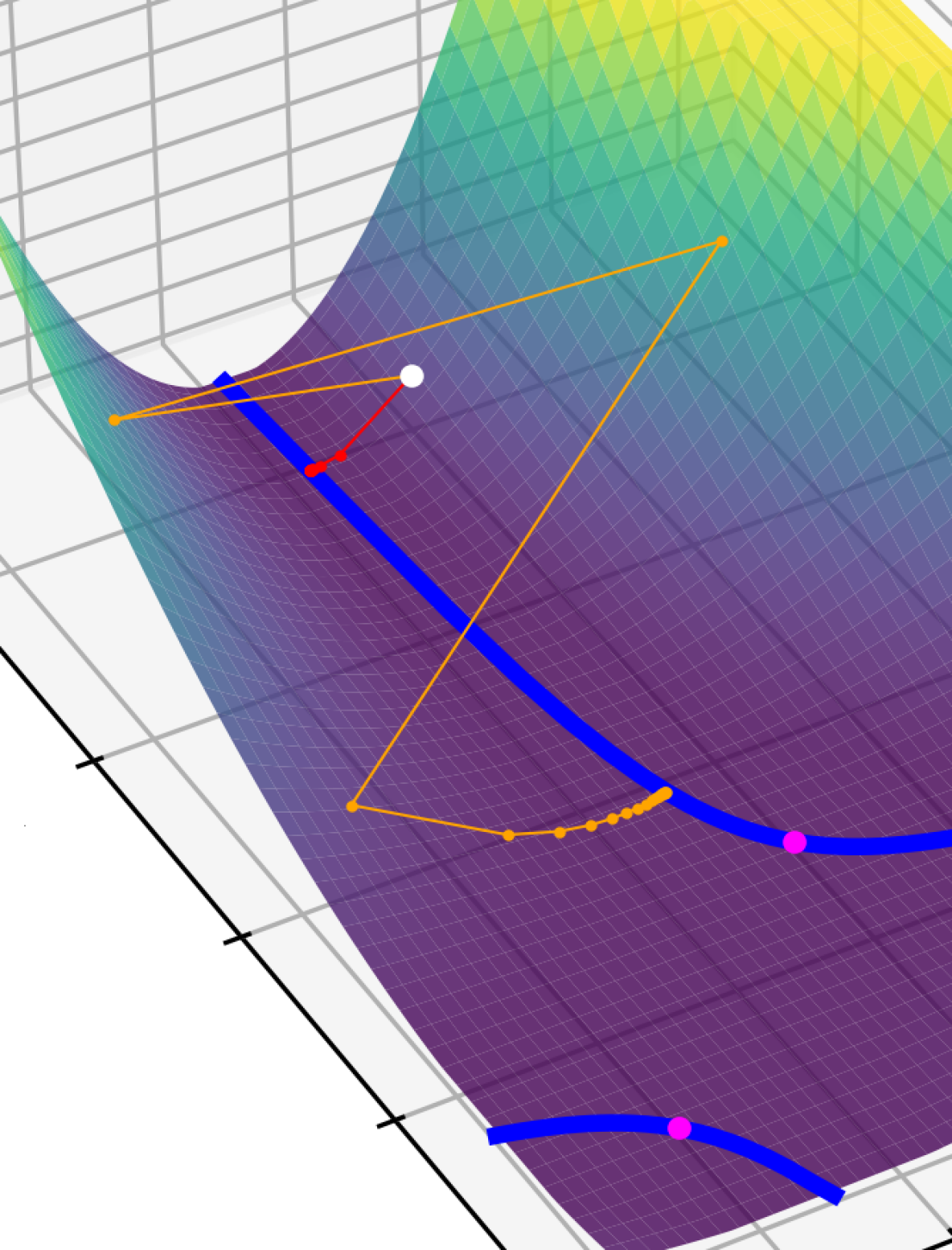
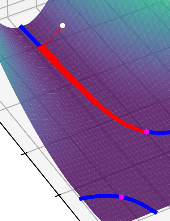
Figure 2: The setting is the same as Fig. 1 outlined in §B. On the left we have the trajectories of full-batch GD for small (red) and big (orange) learning rates. On the right the trajectory of SGD without replacement with small learning rate until convergence. On the left, we see that by increasing the step size, the algorithm identifies a solution closer to the lowest norm one. This implicit regularization effect arises from discretization, consistent with [Lewkowycz et al., 2020, Jastrzębski et al., 2021]. However, no matter the learning rate, we see that GD stops as soon as it gets to a stationary area, while SGD without replacement navigates with an oscillatory trajectory the manifold of minima, converging to the lowest norm one.

The role of the discretization.

Some of the effects of SGD are due to the discretization process. A moderately large learning rate indeed is empirically observed to yield better generalization performance [LeCun et al., 2012, Lewkowycz et al., 2020, Jastrzębski et al., 2021]. This means that the effects of discretization and noise are generally benign. These effects include the one described in [Cohen et al., 2021, Cohen et al., 2022], known as the edge of stability: often GD will start oscillating around the manifold of minima instead of following the gradient flow, while anyway steadily converging [Damian et al., 2023]. All this suggests that a relevant analysis must allow for:

1. Non-vanishing yet finite learning rate.

1. A large Hessian, or alternatively, $(learning\ rate)\cdot Hessian>1$.

In classical numerical analysis, the effects of discretizing differential equations have been studied for long. A useful tool for that [Hairer et al., 2006, Chapter IX] is backward error analysis, introduced with the pioneering work of [Wilkinson, 1960]. While in the 1990s it was used to study the stability of the discretizations, these techniques have been recently used to tackle implicit regularization of GD [Barrett and Dherin, 2021], SGD without replacement [Smith et al., 2021], SGD with momentum [Ghosh et al., 2023], Adam [Cattaneo et al., 2023]. Unfortunately, this line of work usually applies to small step sizes. This article attempts to get around this limitation.

The role of the noise.

The noise of SGD has been considered by numerous authors as a potential factor for explaining generalization in neural networks. Empirically, both the size of the noise [Keskar et al., 2016, Jastrzębski et al., 2018] and the shape or direction of the noise indeed play crucial roles [Wen et al., 2019, Smith et al., 2021]. That said, despite extensive research on this phenomenon, it remains an enigmatic aspect of deep learning theory and needs further investigation.

1. The noise at every step is not Gaussian, does not admit lower bounded variance, etc. In particular, it vanishes in the global minima and it has a shape and a structure.

What we do know from physics and mathematics is that the fact of having random diffusive fluctuations implicitly biases the dynamics towards flatter areas. This is a well-known phenomenon in physics called thermophoresis, and it is mathematically explained with Fokker-Plank-like equations. There are many works in the ML community about this kind of effect, most notably [Chaudhari and Soatto, 2018, HaoChen et al., 2020, Orvieto et al., 2023, Chen et al., 2023]. That said, these papers are about dynamics where the noise is regular and well-behaved, e.g. every step is independent, the noise does not vanish along the trajectories, etc. In particular, they are dealing with injections of Gaussian noise or dynamics assimilable to geometric Brownian motions. While some of these results, in some settings, it is claimed to apply to SGD with replacement, to the knowledge of the author it was proved neither mathematically, nor empirically. Moreover, as far as we know, there exists no diffusion-related result applicable to SGD without replacement, nor any empirical observation that that may be the case.

Probably the most common approach in deriving the effect of the noise is by taking the limit SDEs derived from gradient flows. This is the case of, e.g., [Li et al., 2017, Chen et al., 2023]. Unfortunately, SDE approximation limit is always ill-posed [Yaida, 2018] and on top of that never behaves as SGD apart for extremely particular cases, as very small learning rate for scale-invariant neural networks in a setting in which the variance is bigger than the gradient [Li et al., 2021]. Moreover, [Li et al., 2021] questioned the applicability of CLT in this context, so we are not even sure in what terms we can speak of these diffusion-powered effects. On top of all the above, [HaoChen et al., 2020] showed the differently shaped noises (Langevin dynamics, label noise, etc.) converge to different minima even though as the effect of diffusions. On top of these limitations of the approach, all this work is only about SGD with replacement.

Finally, [Smith et al., 2021] provides further empirical and theoretical evidence that this SDE approach should not work in explaining the effect of SGD without replacement. Moreover, [Damian et al., 2021, Li et al., 2022] show that even in the case of diffusive independent noise at every step, as label nose injection or SGD with replacement, the implicit regularization effect is due to drifts coming from the higher order terms in Taylor, not from the diffusion-powered regularization. Thus, to understand the true impact of SGD noise on neural networks, a relevant analysis should account for the fact that:

1. The noises of different steps are not independent, nor centered.

In particular, the randomicity of SGD without replacement is smaller than what people expect. In SGD without replacement, the noise comes from reshuffling the dataset once every epoch, not from sampling at every step. The batches are disjoint, thus dependent, and given the first $k-1$ the $k-th$ is deterministic. Another way to look at this is to think that our steps, or the observations of the random variable mini-batch gradient, are exchangeable but not independent. There exists plenty of work on the (dis)similarity of a set of exchangeable vs independent random variables, starting with the De Finetti theorem.

2.4 The Real-World Regime

The product $c:=\eta\cdot k$ between the learning rate and the number of steps in an epoch plays a crucial role in the effect of SGD. Empirically, for instance, studies found that the size of the SGD effect scales with $c$, or analogously with

$$\frac{\eta}{b-1}\quad=\quad\frac{c}{n}.$$

This is the so-called linear scaling rule in the literature [Goyal et al., 2017, Jastrzębski et al., 2018, He et al., 2019]. Predictably, $c$ comes out in our regularizer too, see Eq. 3 or Theorem 1, for instance. From a theoretical point of view, the reason is that we can rewrite the Taylor expansion as sum of products of $c$ times the derivatives. Precisely, the factors appearing are of the form $c\cdot\nabla^{i}L$, so for instance the first terms can be rearranged as

$$-\ \eta k\nabla L\ +\ \eta^{2}\binom{k}{2}\nabla^{2}L\nabla L\ -\ \eta^{3}\binom{k}{3}(\nabla^{2}L)^{2}\nabla L\ +\ \ldots$$

In every term $\eta$ and $k$ appear multiplied to the same order, thus this can be rewritten approximately as

$$-\ c\nabla L\ +\ \frac{c^{2}}{2}\nabla^{2}L\nabla L\ -\ \frac{c^{3}}{6}(\nabla^{2}L)^{2}\nabla L\ +\ \ldots$$

With an approximation error of $O(1/k)$. For this reason, most analyses require $c=\eta\cdot k$ to be much smaller than $1$, or analogously $c\nabla L,c\nabla^{2}L\ll 1$. This is the case for instance of [Smith et al., 2021, Roberts, 2021].

In practice, however, this is not usually the case and $c$ or $c\nabla^{2}L$ are not small. As an example, MNIST and CIFAR10 datasets have, respectively, $n=60,000$ and $n=50,000$ training examples. With a batch size $b$ of 32 or 64, we would have values of $k$ ranging between $800$ and $1900$, so of order of magnitude $10^{3}$. Common choices for $\eta$ range from 1 or 0.1 at the beginning of training, decreasing to 0.01 or 0.001 towards the end. This results in values of $c=\eta\cdot k$ ranging between hundreds initially, to values between $0.8$ and $10$ later on.

Dataset	Model	$\begin{subarray}{c}\text{Training}\\ \text{set size }n\end{subarray}$	$\begin{subarray}{c}\text{Step sizes }\eta\end{subarray}$	$\begin{subarray}{c}\text{Batch size }b\end{subarray}$	$\begin{subarray}{c}c\ =\ \eta\cdot k\end{subarray}$
MNIST	MLP	60k	0.1 - 0.01	32-64	190 - 9.4
Cifar10(0)	DenseNet-BC-190	50k	0.1 - 0.001	64	78 - 0.8
Cifar100	ResNet-BiT	50k	0.03 - 0.0003	4096	0.36 - 0.004
ImageNet	ResNet152	1.2M	0.1 - 0.001	256	470 - 4.7

Note that in most of the cases in the table above, SGD is equipped with momentum with $\beta=0.9$. This implies that the effective step is bigger:

$$\eta\ (1+0.9+0.81+\ldots)\quad=\quad 10\cdot\eta$$

making the effective $c$ ten times bigger. The only element of the form $c\nabla^{i}L$ that we can be sure tends to become small during the middle and later stages of training is thus $\eta k\nabla L$, as the gradient approaches zero and the learning rate, $\eta$, gets annealed. However, the same can not be said of the second or the third derivative [Cohen et al., 2021, Damian et al., 2023].

Variants of SGDs on Toy Shallow Networks

Figure 3: We trained shallow networks of the first 10k examples of cifar10 using SGD without replacement with learning rate $\eta=0.01$ and various batch sizes. We plotted the size of the biggest eigenvalue at the beginning of the training and at the end. At the end of training $\|c\nabla^{2}L\|$ ranges between 150 for $b=128$ and 437 for $b=32$. In particular, we are in the hypothesis of our results but not in the hypothesis of previous research.

3 Implicit Bias of SGD Without Replacement

Many past studies have shown how different algorithms perform in different settings, and which minima they converge to. We want to understand to what extent these results can or can not be applied to SGD without replacement. After setting the notations in §3.1, we investigate the expectation of the deviation between trajectories of SGD without replacement and other algorithms in §3.2.

Technically our analysis works as follows, see §D:

• Deviation: We first compute the deviation between trajectories 9.

• Moments: Then we determine its moments with the machinery developed in the appendix §E.

3.1 Notations

We denote by $D=\{z_{i}\}_{i=1,2,\ldots,n}\subseteq V$ the training set of size $n$. We have a parametric loss function $L\colon(\vartheta,z)\mapsto L(\vartheta,x)\in\mathbb{R}$ that takes as input the parameters $\theta\in\Theta$ and the data $z\subseteq V$ and outputs a real number, admitting 3 weak derivatives in the parameters $\vartheta$. For every set $B\subseteq V$ we define $L(\vartheta,B):=\tfrac{1}{|B|}\sum_{z\in B}L(\vartheta,z)$. The goal of the optimization procedure is to find a minimum $\theta^{*}\in\Theta$ for the objective function $L(\vartheta,D)$.

For readability, we will often omit the inputs of the function $L$. Precisely, whenever we omit the parameter $\vartheta$ we are evaluating the loss at the beginning of the epoch, we will denote the value of the parameters at the beginning of the epoch with $\theta$. Whenever we omit the set of inputs we are evaluating the loss over the whole training set $D$. Moreover, all the derivatives we will take will be in the parameters $\vartheta$ and all the expectations will be empirical expectations over a set $B\subseteq V$. As an example

$$L\text{ means }L(\theta,D)\quad\quad\text{and}\quad\quad\nabla L(B)\text{ means }\nabla_{\theta}L(\theta,B).$$

Moreover, we will denote by $\theta_{i}^{SGD}$ the parameters after the $i-th$ step of SGD without replacement or, analogously, of Shuffle Once (SO) starting from $\theta_{0}^{SGD}=\theta$ with learning rate $\eta>0$. In this section, we will take also other algorithms in exam, such as SGD with replacement, GD, or GD with noise injected. Analogously to SGD without replacement, we will denote by $\theta_{i}$ the parameters after the $i-th$ step of the other algorithms in exam, with initialization $\theta_{0}=\theta$ and the learning rate $\eta>0$.

Let $b\in\mathbb{N}$ be the batch size and $k\in\mathbb{N}$ the number of optimization steps considered at once. Generally, $k\leq n/b$ will be, and can be thought of as, the number of batches or the number of steps in an epoch. We denote by $B_{i}\subseteq D$ the batch used in the $i-th$ step, $i\leq k$. Denote by $c:=\eta k$ and by $H:=\frac{c^{2}}{2n}\big{(}\mathbb{E}[(\nabla^{2}L)^{2}]-(\nabla^{2}L)^{2}\big{)}$. Finally, we denote by $A^{\dagger}$ the Moore-Penrose inverse of the matrix $A$ and, for a PSD matrix $S$, we denote $\|v\|_{S}^{2}:=v^{\top}Sv$. For a vector or matrix we denote the components with the indices in subscripts, e.g., for $A\in\mathbb{R}^{d\times d}$, for $i,j\leq d$, we denote $A_{i,j}$ the $(i,j)$ component of the matrix $A$.

3.2 The Trajectories are Biased

One epoch or less at once, we analyze the optimization dynamics. We show that relative to full-batch GD or SGD with replacement, SGD without replacement and shuffle once implicitly add a step on a regularizer that penalizes a function of the variance of the loss gradients. It is important to note that this is not the first such result. Indeed [Roberts, 2021] showed earlier that SGD has an implicit bias and gave some insights on the generalization benefits of it, while [Smith et al., 2021] showed that in a small learning rate regime, precisely $c\nabla^{2}L\ll 1$ and $H\ll 1$, SGD without replacement in expectation follows a gradient flow on a modified loss.

The regularizer we find is essentially the sum of variances of the gradient noise measured in a loss-dependent norm determined by the Hessian of the loss. Precisely, 9 analyzes the deviation of any mini-batch algorithm from GD, Theorem 3 and Theorem 2 specializes to SGD without replacement and to shuffle once. Precisely, Theorem 2 works in the general case, while Theorem 3 is cleaner but specializes in the setting in which $\eta\nabla^{2}L$ has only small and big eigenvalues, not in between.

Theorem 2.

In the notations of §3.1, let $\theta_{i}$ be the parameters after $i$ steps of any algorithm with independent steps centered on the GD step. These being, e.g., SGD with replacement, GD, label noise GD, Gaussian noise injected GD, etc. Let us assume that $\eta k\nabla L(.)\ll 1$. Then up to a multiplicative error of size $\eta^{\alpha}k\nabla L+1/n$ with $\alpha\geq 1$. In expectation over batch sampling, $k$ steps of SGD without replacement differs from the same number of steps of SGD with replacement or GD, $\mathbb{E}[\theta_{k}]$ by additional preconditioned steps with learning rate $\tfrac{\eta}{b-1}$ on some regularizers.

$$\mathbb{E}_{\left[\begin{subarray}{c}\text{expectation over}\\ \text{batches' sampling}\end{subarray}\right]}\left[\theta^{SGD}_{k}\right]\quad=\quad\mathbb{E}[\theta_{k}]\quad-\quad\frac{\eta}{b-1}\ \sum_{i=0}^{k-2}A_{i}\nabla\text{Regularizer}_{i}$$

where $A_{i}=(-\eta\nabla^{2}L)^{i}$ and

$$\text{Regularizer}_{i}\quad=\quad\mathbb{E}_{z\in D}[\|\nabla L(z)-\nabla L\|_{S_{i}}]\ +\ \nabla L^{\top}\mathcal{S}_{i}\nabla L.$$

Where the matrices $S_{i}$, $i\leq k-2$, and $\mathcal{S}$ are series of powers of the loss $\nabla^{2}L$ and $H$.

Analogously, let us fix an orthonormal basis $\{\theta_{1},\theta_{2},\ldots\}$ of eigenvectors for the Hessian $\nabla^{2}L$. In the case in which $H\ll 1$ at $\theta$ stationary point, we can rewrite this bias along the eigenvector $\theta_{i}$ corresponding to the eigenvalue $\lambda_{i}$ as

$$-\frac{\eta}{b-1}\ \sum_{j}R_{i,j}\ \frac{d}{d\theta_{i}}Cov_{z\in D}(\nabla L(z))_{j,j}$$ (4)

where

$$R_{i,j}\quad=\quad\frac{1}{2}\sum_{h=0}^{k+2}(-\eta\lambda_{i})^{h}\sum_{l=h+2}^{k}\binom{k}{l}(-\eta\lambda_{j})^{l-h-2}.$$ (5)

Note that the entries $R_{i,j}$ are approximately

$$R_{i,j}\quad\sim\quad\frac{c}{2}\cdot\begin{cases}\frac{1}{2}\!\!\qquad\qquad\qquad\qquad\qquad\quad\text{ constant}\qquad&\text{ if }c\lambda_{i},c\lambda_{j}\text{ small}\\ (c\lambda_{i})^{-1}\hskip 1.13791pt\quad\qquad\qquad\quad\qquad\text{ small}&\text{ if }c\lambda_{i}\gg 0,c\lambda_{j}\text{ small}\\ (c\lambda_{j})^{-1}\quad\qquad\qquad\qquad\quad\text{ small}&\text{ if }c\lambda_{i}\text{ small},c\lambda_{j}\gg 0\\ \frac{1+(-\eta\lambda_{i})^{k}}{c\lambda_{i}\cdot c\lambda_{j}}\quad\qquad\qquad\qquad\ \,\begin{subarray}{c}\text{very small }\\ \text{or very big}\end{subarray}&\text{ if }c\lambda_{i},c\lambda_{j}\gg 0\\ \Omega\big{(}(c\lambda_{j})^{-2}\exp(-c\lambda_{j})\big{)}\qquad\begin{subarray}{c}\text{exponen-}\\ \text{tially big}\end{subarray}&\text{ if }c\lambda_{j}\ll 0\end{cases}$$ (6)

We can now leverage this way to write a corollary that corresponds to Theorem 1:

Theorem 3.

In the notations of §3.1 up to a multiplicative error of size $\eta^{\alpha}k\nabla L+\|H\|+1/n$ with $\alpha\geq 1$. Let us work in the coordinate of a basis of eigenvectors $\{\theta_{1},\theta_{2},\ldots\}$ for $\nabla^{2}L$. After $k$ steps of SGD without replacement we have $k$ steps of GD plus an additional step as follows. At a stationary point, the step due to the bias on $\theta_{i}$ corresponding to the eigenvalue $\lambda_{i}$ is

$$-\frac{\eta}{b-1}\ \sum_{j}R_{i,j}\frac{d}{d\theta_{i}}\operatorname{Cov}_{z\in D}(\nabla L(z))_{j,j}.$$

The proof of these results can be found in the appendix. We will give a deeper look into the nature of the regularizer in §7 and of the matrices $S_{i}$s in 20. We deal with the error and the regimes in which Theorems 3 and 2 apply in §J.

3.3 Small Learning Rate or Small Hessian Regime.

Assume that the full-batch Hessian $c\nabla^{2}L$ is small, but we have arbitrary "variance" $H$, and $\theta$ at the beginning of the epoch is close to a stationary point. Then we can conclude that the regularizer’s step coincides with

$$-\frac{\eta}{b-1}\nabla\mathbb{E}_{z\in D}[\|\nabla L(z)-\nabla L\|_{S_{0}}]$$

where $S_{0}$ is

$$S_{0}\quad=\quad\frac{c}{4}H^{-1/2}\sqrt{\pi}\ \mathrm{erf}(\sqrt{H})\left(2+2H^{-1/2}(e^{-H}-1)-c\nabla^{2}L\right).$$

When $H\ll 1$ this becomes approximately $S_{0}=\frac{c}{4}I$ and the regularizer is

$$\frac{c}{4}\operatorname{\mathbb{V}ar}{\|\nabla L\|}.$$

This aligns with prior theoretical findings by [Smith et al., 2021] and empirical findings by [Jastrzębski et al., 2021]. More about the exact formula of the matrices $S_{i}$ can be found in 20.

4 Shaping the Hessian

In this section, we show that SGD without replacement implicitly regularizes by the variance of the gradients. We find that Theorem 2 is potentially enough to explain several empirically observed phenomena about implicit regularization, e.g., that:

• SGD converges to almost-global loss minima even though spurious minima of the loss exist [Dauphin et al., 2014, Safran and Shamir, 2018, Zhang et al., 2022].

• SGD shapes the spectrum of the Hessian of the loss, e.g., producing clusters of large outlying eigenvalues and sending small eigenvalues to zero in the course of training [Keskar et al., 2016, Sagun et al., 2016, Papyan, 2020, Jastrzębski et al., 2021].

We show indeed that it biases the dynamics in areas where there is (i) lower variance, (ii) the landscape is flatter, (iii) the model better fits the data, and (iv) it oscillates less. Moreover, we later give heuristics about how it regularizes the spectrum of the Hessian/Fisher Matrix.

4.1 Empirical Observations

One of the papers that started the whole line of research on the implicit bias of algorithms was [Keskar et al., 2016]. They observed that in the experiments a lower batch size led, generally, to a wider (or less sharp) minimum. Precisely, they observed that the minima found by lower batch sizes have an Hessian with a smaller number of large eigenvalues, or a smaller trace. Analogously, we find that the small eigenvalues that do not carry information about the problem get zeroed out. A recent paper, [Jastrzębski et al., 2021], shows experimentally that big learning rate SGD has an effect similar to penalizing

$$\mathrm{trace}\!\left(\mathbb{E}\left[\nabla L\nabla L^{\top}\right]\right)\quad=\quad\mathbb{E}\left[\|\nabla L\|^{2}\right]$$

that in the image classification task in which they work coincides with the trace of the Fisher matrix. In related settings, the Fisher matrix has been shown to approximate the Hessian during the training; in particular, there is an overlap between the top eigenspaces of the Hessian and its eigenspaces [Jastrzębski et al., 2018, Martens, 2020, Thomas et al., 2020]. Furthermore, [Jastrzębski et al., 2021] shows that, in practice, penalizing it consistently improves generalization, reduces memorization, and regularizes the trace of the final Hessian. Moreover, the advantages of penalizing the trace of the Fisher matrix are even stronger when in the presence of noisy labels. There exist multiple other studies along these lines, and in particular corroborate our findings. Some recent ones are [Lu et al., 2023] who observe that a bigger learning rate "prevents the over-greedy convergence and serves as the engine that drives the learning of less-prominent data patterns", this aligns with the regularization phenomenon that we unveil. Analogously, [Geiping et al., 2021] showed how full-batch GD strongly regularized perform as SGD explicitly using a penalization very similar to the regularizer we find and in line with [Smith et al., 2021].

4.2 The Regularizer

SGD without replacement regularizes the noise covariance in the eigendirections corresponding to smaller eigenvalues.

Near a stationary point, the regularizer step is approximately

$$\frac{\eta}{b-1}\ \cdot\ \sum_{i=0}^{k-2}\ (\eta\nabla^{2}L)^{i}\ \cdot\ \nabla_{\theta}\left(\text{trace}\left(S_{i}\cdot\operatorname{Cov}_{z\in D}(\nabla L(z))\right)\right).$$

We can thus interpret it as a sequence of steps, one for each $i$, of size $\eta/b$ with preconditioning matrix $(\eta\nabla^{2}L)^{i}$ on the regularizers

$$\mathbb{E}_{z\in D}\left[\|\nabla L(z)-\nabla L\|_{S_{i}}^{2}\right]\quad=\quad\text{trace}\left(S_{i}\cdot\operatorname{Cov}_{z\in D}(\nabla L(z))\right).$$

The matrices $S_{i}$ from Theorem 2 are small (essentially zero) in all eigendirections of the Hessian of the loss corresponding to large positive eigenvalues. In contrast, in the eigendirections associated with small positive eigenvalues, the $S_{i}$s are considerably larger. Precisely, if for a certain eigenvalue $\lambda$ of the Hessian $\nabla^{2}L$ we have $|c\lambda|\ll 1$ we can essentially look only at the term with $S_{0}$ and we have that the approximate regularizer along the eigendirection of $\lambda$ coincides with a penalization of the noise covariance or analogously of the norm of the gradients

$$\frac{c^{2}}{4}\ \mathbb{E}_{z\in D}\left[\|\nabla L(z)-\nabla L\|^{2}\right]\quad=\quad\frac{c^{2}}{4}\ \text{trace}\left(\operatorname{Cov}_{z\in D}(\nabla L(z))\right).$$

On the other hand, in the eigendirections of big eigenvalues $c\lambda\gg 1$, but $\eta\lambda\leq 1$, the effect of the regularizer still penalizes the noise covariance but with an intensity that is continuously decreasing in $\lambda$. The size of the step shrinks as $O\big{(}\lambda^{-1}\big{)}$ becoming essentially very small when the big eigenvalues approach big $O(\eta^{-1})$ values.

This implies that SGD without replacement implicitly regularizes mainly along the eigenspaces of the small and negative eigenvalues of the Hessian, which are considered to control (i) how the model overfits and (ii) the effective complexity and sparsity of the model.

4.3 Variance, Global Minima, and Flatter Models

We showed that the regularizer acts by reducing the variance in the eigendirections of the smaller eigenvalues. We discuss here a correspondence between optimizing the regularizer and finding better minima Smaller variance
$\iff$
Smaller norm of the gradients
$\iff$
Better fitting and/or flatter minima. In the previous subsection we showed that when $\theta$ is close to a manifold of stationary points, the regularizer pushes the trajectory towards areas with lower variance. It is important to note that the quantity we dealt with has many different interpretation

$$\text{trace}\big{(}\mathbb{E}\big{[}\nabla L(z)\nabla L(z)^{\top}\big{]}\big{)}\quad=\quad\underbrace{\mathbb{E}_{z\in D}\left[\|\nabla L(z)-\nabla L\|^{2}\right]}_{\text{Noise Variance}}\quad=\quad\mathbb{E}_{z\in D}\big{[}\underbrace{\|\nabla L(z)\|^{2}}_{\begin{subarray}{c}\text{Gradients'}\\ \text{Norm}\end{subarray}}\big{]}$$

In particular, let the loss be of the form $L=\ell\circ f$ and denote by $\nabla\ell=\frac{d\ell(z)}{dz}|_{z=f(\theta,x)}$ the residuals. E.g., $L(\theta,z=(x,y))=\|f(\theta,x)-y\|^{2}$ with $\nabla\ell=f(\theta,x)-y$ for MSE. We have that

$$\mathbb{E}_{z\in D}\left[\|\nabla L\|^{2}\right]\quad=\quad\mathbb{E}_{z\in D}\left[\nabla_{\theta}f^{\top}\|\nabla\ell\|^{2}\nabla_{\theta}f\right].$$

So at every step, we penalize what essentially is the sum over the output components $i$ of products of $\|[\nabla f]_{i}\|^{2}$ and $\|[\nabla\ell]_{i}\|^{2}$, i.e., the residuals and norm of the gradient of the model on the components of the output. When the dimension of the outputs is one, this is exactly $\|\nabla\ell\|^{2}\|\nabla_{\theta}f\|^{2}$. This corresponds to lowering the size of $\nabla\ell$s and/or the size of $\nabla_{\theta}f$. Thus if we lower the variance we lower this product and if we lower this product we lower the variance. This implies that, with different weights given by the PD matrices $S_{i}$s, the regularizer pushes towards areas where either $\|\nabla\ell\|^{2}$ or $\|\nabla_{\theta}f\|^{2}$ are smaller.

The regularizer pushes towards locations in parameter space where either: 1) The squared residuals $\|\nabla\ell\|^{2}$ are smaller.
I.e., it escapes towards a better-fitting stationary point, as a global minimum, or 2) The gradients of the model $\|\nabla f(\theta,x)^{2}\|$ are smaller.
This, in turn, may correspond to wider valleys and may correspond to a smaller norm of the gradient in the inputs $x$ of the function $f$. Thus potentially finding a better generalizing minimum by making the function represented by the neural network less oscillating and less prone to overfitting and memorization.

This effect was not observed in previous works, to the knowledge of the author and is the opposite of what we expect from full-batch GD, since [Cohen et al., 2021, Appendix C] observed that along the trajectory of $\|\nabla f(\theta,x)^{2}\|$ keeps steadily increasing. Nonetheless, it agrees with empirical observations.

Evidences of Regularization: SGD Escapes Local Minima

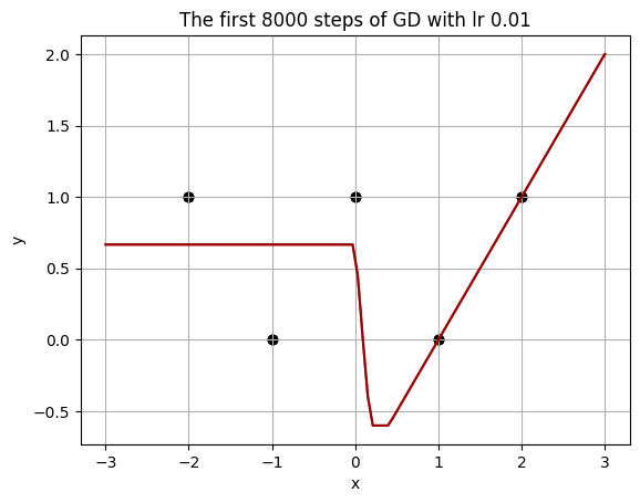
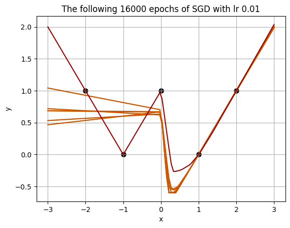
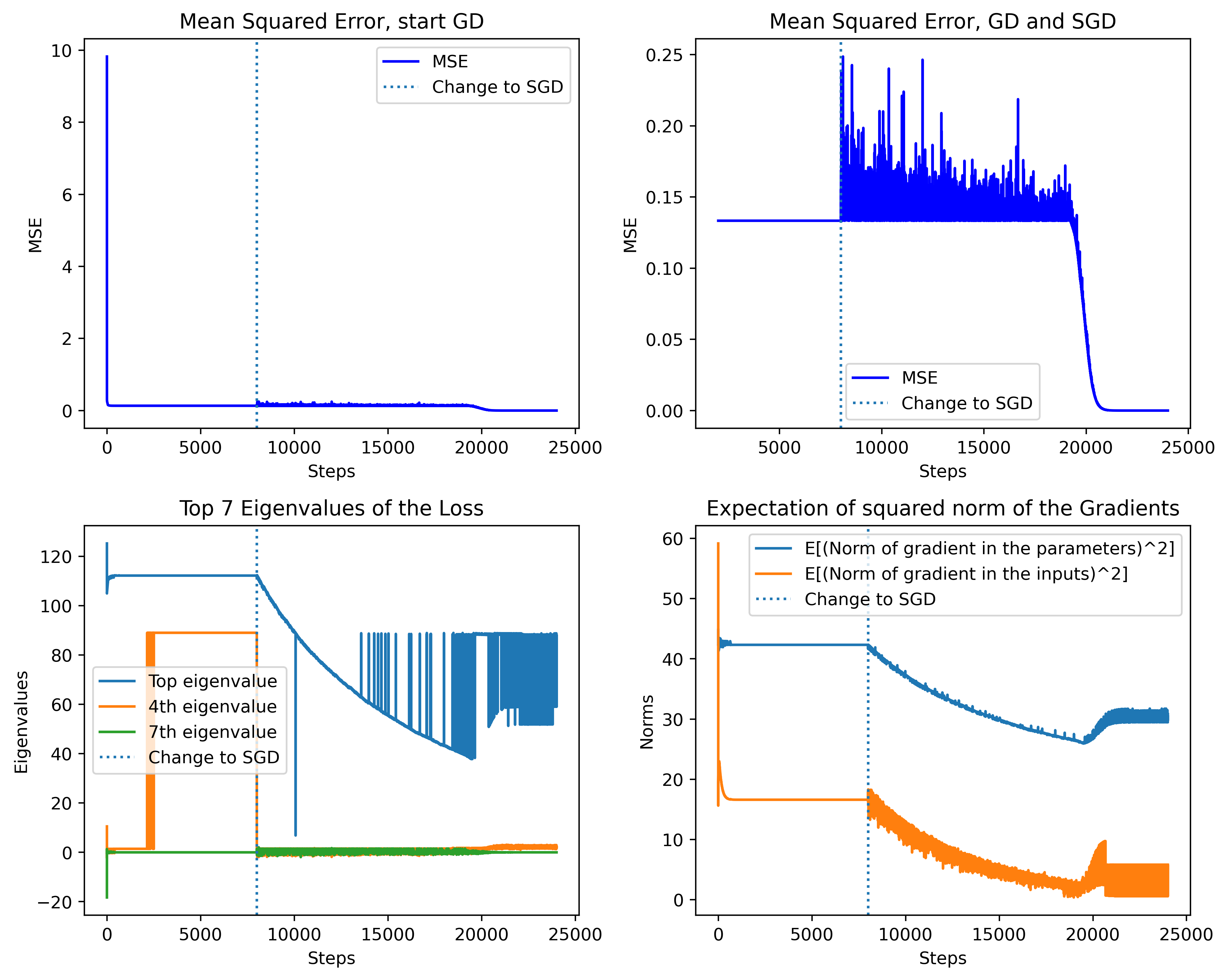
Figure 4: We see here the SGD without replacement escapes local minima to which GD converged. Precisely, it escapes them in directions in which it optimizes the regularizer. Thus shrinking the eigenvalues and the norm of the gradients, before the loss.
We fit "W" shaped one-dimensional data points with a shallow-ReLU network and MSE. We run 8000 steps of GD with learning rate $\eta=0.01$ and it converges to the function represented to the right (in less than 400 steps). This point is a minimum, not a saddle. It is a local (non-global) minimum. We then run 16000 epochs of SGD with the same learning rate and batch size 2. SGD escapes the local minimum in directions in which it optimizes the regularizer and converges to a global minimum. We can see below that the MSE of the local minimum found by GD was $\sim 0.14$, while the MSE at the global minimum found by SGD is $2.5e-12$. The orange functions above are the functions represented by the neural network after 100, 800, 2000, 4000, 6000, and 8000 epochs, the red function is the function of the neural network at convergence. It is noticeable how the top eigenvalue of the Hessian, the gradients of the model in the parameters space, and the gradient of the models in the inputs start shrinking as we change the optimization algorithm and follow similar trajectories.

4.4 Regression and Oscillations

Variance and Hessian in Regression.

Note that, in the case $L=\ell\circ f$, the Hessian of the loss $\nabla^{2}L$ consists of two parts, precisely:

$$\nabla^{2}L\quad=\quad\nabla^{2}\ell\ \nabla f\ \nabla f^{\top}\ +\ \nabla\ell\ \nabla^{2}f.$$ (7)

The first summand has linear combinations of $\nabla f$ as eigenvectors and linear combinations of $\|\nabla f\|^{2}$ as eigenvalues. If the $\nabla f$s are orthogonal, those are exactly the eigenvalues and eigenvectors, this is the case of orthogonal data in shallow linear networks, for example. Analogously, the second part is of size $\nabla\ell$ and when the algorithm converges, in general, it is observed to vanish. In particular, it is $0$ at a global minimum. This means that SGD without replacement implicitly regularizes on the Hessian matrix. Precisely, it prefers sparse Hessians to approximately sparse Hessians, making smaller the already small eigenvalues. Moreover, this also implies a shrinking in the input gradient of the function $\nabla_{x}f(\theta,x)$ as those are related §M.

4.5 Classification: Trace of the Hessian

Towards explaining the empirical observations.

Theorem 2 potentially explains and formalizes why [Jastrzębski et al., 2021] empirically observed that a higher effective learning rate $\eta/b$ (corresponding to bigger steps on the regularizer) better regularizes the trace of the Fisher matrix, in vision classification tasks. In particular, thanks to Theorem 4 we prove that, once most training points are correctly classified, SGD without replacement effectively minimizes a weighted trace of the Hessian. Indeed the regularizer corresponds to

$$\text{trace}\big{(}S\,\cdot\,\underbrace{\mathbb{E}\big{[}\nabla L(z)\nabla L(z)^{\top}\big{]}}_{\begin{subarray}{c}\text{Empirical}\\ \text{Fisher Matrix}\end{subarray}}\big{)}\quad=\quad\text{trace}\big{(}S\,\cdot\,\nabla^{2}L(\theta,D)\big{)}$$

This is the first mathematical result, to the knowledge of the author, that explains and formalizes the observation of [Keskar et al., 2016]. Moreover, this potentially explains frequent observations that SGD tends to discover minima with a sparsified Hessian, characterized by a few outlying large eigenvalues (although smaller than $\eta^{-1}$) and many smaller eigenvalues near zero, see, e.g., [Keskar et al., 2016, Sagun et al., 2016, Papyan, 2019].

Hessian corresponds to Fisher.

[Thomas et al., 2020] showed that the trace of the Hessian is approximately the trace of the Fisher matrix along the learning trajectory of image classification tasks. The surprising part of [Thomas et al., 2020] is that this is the case along most of the trajectory and not only in the final part, as shown by the following theorem. This means that generally in the first part of the training SGD already correctly learns the vast majority of the labels and the major part of the learning is just regularization by SGD and other elements of the training.

Theorem 4 (Regularizing the trace of Hessian).

Assume all the training data are correctly classified and we use cross-entropy loss. Then

$$Fisher\quad=\quad\mathbb{E}_{z\in D}[\nabla L\nabla L^{\top}]\quad=\quad\nabla^{2}L\quad=\quad Hessian.$$

In particular, the local minima of $\text{trace}(S\cdot\text{Fisher})$ coincides with the local minima of $\text{trace}(S\cdot\text{Hessian})$.

The regularizer penalizes the trace of the Hessian.

Theorem 4 and Theorem 2 imply that when $\theta$ is around the manifold of minima for the loss, the regularizer of Theorem 3 acts directly on the Hessian. Indeed, it corresponds in this setting to a number of steps of size $\eta/b$ preconditioned by $(\eta\nabla^{2}L)^{i}$ on

$$\text{trace}\big{(}S_{i}\cdot Cov(\nabla L)\big{)}\quad=\quad\text{trace}\big{(}S_{i}\cdot\nabla^{2}L\big{)}.$$

This means that SGD without replacement biases the dynamics by regularizing the trace of the Hessian, $trace(\nabla^{2}L)$, and in particular it regularizes more heavily the small eigenvalues.

Concluding.

SGD without replacement does not simply penalize the trace of the Fisher matrix or Hessian, but rather targets a weighted trace, with a focus on diminishing the smaller eigenvalues while leaving the larger ones relatively unaffected. This approach aligns with empirical findings where the Hessian’s spectrum typically features a few large eigenvalues amidst many smaller ones (bulkization) [Keskar et al., 2016, Sagun et al., 2016, Martin and Mahoney, 2018, Papyan, 2019, Papyan, 2020]. The larger eigenvalues, carrying crucial information about the problem [Papyan, 2020], are preserved, whereas the smaller eigenvalues, often associated with overfitting and memorization, are effectively targeted by this regularization approach. Consequently, this technique may enhance generalization beyond the simple trace of the Hessian or Fisher matrix. Additionally, this agrees with the observations in §B and what is illustrated in Figs. 1 and 4.

5 Saddles

We believe we make an important step in understanding why and how SGD without replacement escapes saddles so fast in practice. The reason is that the regularizer is simply not affected by most saddles. This is a fundamental difference between SGD with replacement and noise GD, which escape saddles only thanks to the diffusion of the noise.

5.1 Literature Review

Saddles are there.

Many theoretical works deal with the presence of saddles in the loss landscape of neural networks. For instance [Baldi and Hornik, 1989] proved that in the landscapes of shallow linear networks, all the stationary points that are not global minima are saddle. Later, [Kawaguchi, 2016] proved the same for deeper networks, under more general assumptions on the data, showing also the presence of higher-order saddles. Later, plenty of work, as [Petzka and Sminchisescu, 2020], characterize large families of saddles (and local minima) in the loss landscape, for example in terms of stationary points of embedded smaller neural networks.

Escaping saddles with noise.

Many influential works on the optimization side observed how SGD often empirically escapes them [Dauphin et al., 2014, Goodfellow et al., 2016], even though the time required by GD to escape them may often be exponential [Du et al., 2017]. An important number of influential theoretical work was produced on trying to explain why and how fast variants of SGD escape (at least the strict) saddles and developing new algorithms that provably escape faster. For instance, [Lee et al., 2016] proved that almost surely GD escapes saddles asymptotically, and [Ge et al., 2015, Jin et al., 2017, Jin et al., 2021] proved that injecting Gaussian noise in the gradients makes GD escaping in $O(\lambda^{-2})$ time.

A diffusion-powered escape.

The conclusion of many works is that a noised version of GD can escape saddles if the noise is dispersive, a concept essentially analogous to having the covariance of the noise positive in an escaping direction. This is for instance the case of Gaussian noise injection. In that case, with a high probability, the noise will eventually shoot the trajectory away from the saddles. Away enough that the gradient descent part of the algorithm will have a considerable size [Jin et al., 2021]. Following this idea, under the dispersive noise assumption, [Ge et al., 2015], [Daneshmand et al., 2018], [Jin et al., 2021], and later [Fang et al., 2019] proved that SGD with replacement escapes saddles in $O(\lambda^{-3.5})$ time, for proper choices of hyperparameters. The phenomenon described by these works is diffusive in nature, the reason why SGD with replacement is escaping is about the variance term of the i.i.d. noise of each step. We are not aware of work on SGD without replacement escaping saddles. We, however, conjecture that it is possible to obtain a result similar to the ones above.

5.2 SGD Without Replacement Escapes Faster

We show here that SGD without replacement escapes saddles as well. However, our result is very different in nature from the ones produced in the past. We discover a drift-powered escaping effect, not a diffusive one: SGD without replacement, unlike the other algorithms, escapes saddles simply because the implicit step on the regularizer does not vanish there. The regularizer biases the trajectory in escaping directions, if any is spanned by the gradients.

The great news of this section is thus not that SGD may escape saddles, that was known already. The novelty is the way and the speed in which SGD escapes saddles. It is the nature of the effect that makes SGD without replacement escape saddles. SGD without replacement is thus empowered by two weapons against the saddles issue: (i) we believe that in case of dispersive noise, it escapes with a similar dispersive machinery than [Jin et al., 2021, Fang et al., 2019], although we are not aware of works in this direction; and (ii) the regularizer induces a drift-like effect biasing the trajectory towards escaping directions. The interaction and coexistence of these two effects make SGD without replacement escape faster. Moreover, SGD without replacement escapes even when initialized exactly at saddle points.

Proposition 5 (Escaping strict saddles.).

Let $\theta$ be a higher-order saddle for the loss $L$. Let $v$ be an eigenvector of the negative eigenvalue $\lambda<0$ of the Hessian of the loss. Assume

$$u\quad:=\quad\frac{1}{n}\sum_{z\in D}\langle v,\nabla^{2}L(z)\nabla L(z)\rangle\quad\neq\quad 0.$$

Let us assume also that the third derivative is bounded in a neighborhood of the trajectory. Then, SGD without replacement escapes saddle, i.e., the loss is at least $O(1)$ smaller, after

$$\#\text{epochs}\quad>\quad 2\ \frac{\ln(\eta)+\ln(u)+2\ln(c)-\ln(b)}{c\lambda}.$$

Analogously, SGD without replacement travels flat regions like neighborhoods of high-order saddles thanks to the steps on the regularizer.

Proposition 6 (Escaping high-order saddles.).

Let $v$ be a vector in the kernel of the Hessian of the loss. Assume $\|v\|=1$ and

$$u\quad:=\quad\frac{1}{n}\sum_{z\in D}\langle v,\nabla^{2}L(z)\nabla L(z)\rangle\quad\neq\quad 0.$$

Let us assume also that the third derivative is bounded in a neighborhood of the trajectory. Then, SGD without replacement travels distance $1$ in the direction of $v$, i.e., $\langle\theta^{SGD}_{*}-\theta,v\rangle=1$ in a number of epoch

$$\#\text{epochs}\quad=\quad\frac{2b}{\eta c^{2}u}.$$

And if escaping directions for high-order saddles are spanned by the updates, we escape a higher-order saddle in the same amount of time. This is very surprising as it says that no matter the order of the saddle SGD without replacement travels the region with the same speed.

Proposition 7 (Escaping high-order saddles.).

Let $\theta$ be a higher-order saddle for the loss $L$. Let $v$ an escaping direction in the kernel of the Hessian of the loss. Assume

$$u\quad:=\quad\frac{1}{n}\sum_{z\in D}\langle v,\nabla^{2}L(z)\nabla L(z)\rangle\quad\neq\quad 0.$$

Let us assume also that the third derivative is bounded in a neighborhood of the trajectory. Then, SGD without replacement escapes saddle, i.e., the loss is $O(1)$ smaller, after

$$\#\text{epochs}\quad>\quad\frac{2b}{\eta c^{2}u}$$

independently of the order of the saddle.

5.3 Where is the Catch?

Conflicting results.

The findings of this section appear to conflict with previous work demonstrating the difficulty of escaping saddles. A lot of work in the past, indeed, focused on the difficulty of escaping saddles with gradient-based algorithms, highlighting inherent challenges and inefficiencies of gradient-based methods in navigating the landscape of non-convex optimization. For instance, it has been shown that it is NP-hard to find a fourth-order local minimum [Anandkumar and Ge, 2016]. Moreover, GD has been shown to potentially take exponential time to escape from saddle points [Du et al., 2017]. This slowdown occurs even with natural random initialization schemes and non-pathological functions.

Why SGD does it so fast.

SGD without replacement, however, may escape saddle points very quickly as we showed above. The reason why this makes sense is that it is biased. The bias makes it behave as if the loss was not anymore $L$ but $L$ plus a penalization $P$. Thus in a way SGD without replacement implicitly sees the landscape differently and what are saddles for GD on $L$ may not be saddles at all for SGD without replacement. It is important to notice that 7 could already be proved starting from the main result of [Smith et al., 2021] in the setting in which that result applies.

The limitation.

The saddles that we skip are not saddles from the point of view of the algorithm. This, in turn, comes with new challenges. Indeed, while some saddles are not saddles for SGD, some points that were not saddles for the loss may be seen as saddles by SGD, precisely, those points in which the push of the regularizer is exactly the opposite of the push of gradient descent. For those, all the previous negative results in theory apply.

6 At the Edge of Stability

6.1 Empirical Observations

The Hessian grows.

Another interesting phenomenon is the edge of stability, as known from [Jastrzębski et al., 2019, Jastrzębski et al., 2020, Cohen et al., 2021]. Theoretical work in the setting of classification showed that often gradient flow converges towards infinity in the parameter space. Precisely, in certain settings full-batch GD converges towards infinity but in certain particular directions [Lyu and Li, 2019, Ji and Telgarsky, 2020]. Empirical work similarly shows that gradient flow and gradient descent move towards areas where the Hessian of the loss gets bigger and bigger. Precisely, [Cohen et al., 2021, Cohen et al., 2022] showed that along the trajectories of GD and Adam the largest eigenvalue of the Hessian steadily increases. This stops only when it reaches $2/\eta$ for GD and $38/\eta$ for Adam, as those are the instability thresholds for the algorithms.

SGD induces a smaller Hessian.

However, [Cohen et al., 2021] observed that this is not the case for SGD. [Damian et al., 2023] claims that the reason why SGD does not train at the edge of stability is that the implicit regularizer due to the noise explodes close to the boundary $\lambda_{\max}=2/\eta$ working as a log-barrier. [Jastrzębski et al., 2020], instead, observed that in both regression and vision classification tasks, the trajectory of SGD aligns with the one of GD for a while until a breaking point where it diverges from it and goes in areas of the parameter space where the trace of the Empirical Fisher Matrix is substantially lower. This breaking point arrives earlier for bigger effective learning rates $\eta/b$ and later for smaller ones. In what follows, we formalize this observation.

6.2 Why SGD Does not Reach the Edge of Stability

In summary, what we find is that the divergence after the breaking-point observed by [Jastrzębski et al., 2020] is due to the bias of SGD without replacement that we unveiled in Theorem 2. In most regression settings, however, we observed empirically the log-barrier-like effect, as explained by [Damian et al., 2023]. We can not explain it with our theory and we conjecture that it is due to higher-order terms of Taylor or to the diffusion.

Breaking-point: when and why.

At the beginning of training usually, the size of gradients decreases steadily while often the Hessian grows. This means that, soon after the beginning, the training often enters a regime in which we can apply Theorem 2. In the case in which there are at least 2 eigenvalues $\lambda_{1},\lambda_{2}>\eta^{-1}$, the regularizer’s step from Theorem 3 along $\theta_{1}$ eigenvector of $\lambda_{1}$, see Appendix I, takes the following form up to an exponentially small term.

$$\begin{split}\frac{\eta}{b-1}\ \left[\frac{c}{2}\frac{1+(-\eta\lambda_{1})^{k}}{(c\lambda_{1})(c\lambda_{2})}\right]\ \frac{d}{d\theta_{i}}\operatorname{Cov}_{z\in D}(\nabla L(z))[2,2]\quad+\quad\begin{subarray}{c}\text{Other terms of}\\ \text{the regularizer.}\end{subarray}\end{split}$$ (8)

Or analogously, by exchanging the indexes, we obtain the update on $\theta_{2}$. This means that

Proposition 8 (Breaking point).

Assume we are in the hypothesis of Theorem 2. Assume there exist $\lambda_{1},\lambda_{2}$ eigenvalues of the Hessian $\nabla^{2}L$ with eigenvectors $\theta_{1},\theta_{2}$ such that $\lambda_{2}>\eta^{-1}$, $u:=\nabla\operatorname{\mathbb{V}ar}_{z\in D}(\langle\theta_{2},\nabla L(z)\rangle)>0$, and $\lambda_{1}\geq\eta^{-1}+\alpha_{EoS}$ with

$$\alpha_{EoS}\quad:=\quad\frac{1}{c}\left|\ln\left(\frac{c^{2}\lambda_{1}\lambda_{2}\|\nabla L\|}{u}\right)\right|\quad>\quad\frac{1}{c}\left|\ln\left(\frac{c^{2}\|\nabla L\|}{\eta^{2}u}\right)\right|.$$

Then the additional step on the regularizer described by Theorem 2 is bigger than $k$ steps of GD.

The proof of this proposition is immediate after imposing that the quantity in Eq. 8 is bigger than $k$ steps of GD starting from $\theta$. This phenomenon closely agrees with what was observed empirically by [Jastrzębski et al., 2020] where they call the moment of the phase transition "the break-even point", as for the title of that paper.

Dependence on $\eta/b$.

Moreover, agreeing with the empirical observations by [Jastrzębski et al., 2020], we see that $\alpha_{EoS}(\eta,k)$ is a monotonic decreasing function of $\eta/b$, precisely it goes like its inverse.

$$\alpha_{EoS}\quad:=\quad\frac{1}{c}\cdot\big{(}\text{positive}_{\eta}\big{)}\quad=\quad\frac{b}{\eta}\cdot\frac{1}{n}\cdot\big{(}\text{positive}_{\eta}\big{)}\quad=\quad\frac{b}{\eta}\cdot\big{(}\text{positive}_{\eta}\big{)}.$$

Phase transition.

Moreover, this coincides with a phase transition, not with a slow continuous process, as empirically observed by [Jastrzębski et al., 2020]. Indeed, with $\epsilon:=\frac{|\ln(\eta)|}{c}>0$ we have

$$\begin{subarray}{c}\text{Size of the step}\\ \text{on the regularizer}\end{subarray}\quad=\quad\begin{cases}\Theta(\eta\cdot\text{GD step})\qquad&\text{if }\lambda_{1}=\eta^{-1}+\alpha_{EoS}-\epsilon\\ \Theta(\text{GD step})\qquad&\text{if }\lambda_{1}=\eta^{-1}+\alpha_{EoS}\\ \Theta(\eta^{-1}\cdot\text{GD step})\qquad&\text{if }\lambda_{1}=\eta^{-1}+\alpha_{EoS}+\epsilon\\ \end{cases}$$ (9)

Note that $\epsilon$ is usually $O(1)$ so much smaller than $\eta^{-1}$. For instance, see §2.4, second line of the table, for cifar10 with $\eta=0.01$ and $b=64$ we have that it is smaller than the gain in sharpness due to an epoch.

$$\epsilon\quad=\quad\frac{|\ln(\eta)|}{c}\quad=\quad 0.6.$$

Log-barrier.

Regarding the log-barrier phenomenon, if the optimizer has independent steps with a certain variance, we conjecture that we can apply a version of the results of [Damian et al., 2021, Li et al., 2022] to figure out what the implicit regularization due to the higher-order terms of the Taylor is. In their settings, the effect of the noise is to implicitly add a regularizer to the loss. These regularizers explode as $\lambda_{\max}$ approaches the edge of stability and, for label-noise injection [Damian et al., 2021], it works as a log-barrier. Based on our experiments, we believe that this occurs: (i) when Theorem 2 is not applicable, (ii) in scenarios where $\alpha_{EoS}>\eta^{-1}$, (iii) when the regularizer directs the trajectory into areas of the parameter space that continue to experience progressive sharpening, and (iv) when the remaining terms in the regularizer’s step are sufficiently strong and in the opposite direction, effectively canceling it out. However, this will be the focus of further studies.

7 The Nature of the Effect

We list and discuss here the nature of the effect and how different it is from other effects discovered in the literature. We discuss in the following subsection the two ingredients of the effect: dependency, and discretization. Later we discuss the fact that the effect is a drift, it is not a diffusion-powered effect. We conclude with remarks and observations on the regularizer.

7.1 Discretization

The regularization term that we find Theorem 2 is the expectation of the quantity in 9. 9 is the result of computing the effect of the discretization, it is unrelated to the optimization problem or to the gradient flow itself.

Assume the batches $B_{1},B_{2},\ldots,B_{k}\subseteq D$ are fixed. How far are the trajectories of mini-batch and full-batch GD after $k$ steps of learning rate $\eta$?

We expand $k$ steps of SGD and GD with learning rate $\eta$ at the beginning of the epoch, and we keep the terms in which $\nabla L(\cdot)$ appears to the power 1. We write the difference between this quantity in the case of SGD and the case of GD and we obtain the following

Proposition 9.

Set $B_{1},B_{2},\ldots,B_{k}$ fixed batches of the dataset $D$. The trajectory of mini-batch SGD deviates from the trajectory of the same number of steps $k$ of full-batch GD with the same learning rate $\eta$ of

$$\begin{split}&-\eta\sum_{i=1}^{k}\nabla L(B_{i})\quad+\quad\eta^{2}\sum_{1\leq i<j\leq k}\nabla^{2}L(B_{j})\Bigg{[}\prod_{h=i+1}^{j-1}[I-\eta\nabla^{2}L(B_{h})]\Bigg{]}\ \nabla L(B_{i})\\[5.69046pt] &\quad-\quad\begin{subarray}{c}\text{same terms but full-batch:}\\ B_{j}\curvearrowleft D\text{ for all }j\leq k\end{subarray}\end{split}$$

up to first order in $\eta\nabla L(B_{i})$, $i=1,2,\ldots,k$.

More details about the computation are in the proof in Appendix F and about the size of the error in §J.

7.2 Dependency

The deviation between trajectories is a sum of products of functions evaluated on different batches. Thus the expectation of the difference between the trajectories of a mini-batch SGD and GD is zero when the steps are:

• Centered: every step is a random variable centered in the GD step. E.g., an unbiased estimator of it as for SGD with replacement or some centered Gaussian noise gets injected in the gradient.

• Independent: the steps are random variables independent of each other.

Indeed in that case, the expectations of those products are products of the expectations, in particular full-batch derivatives. This is not the case of SGD without replacement. Indeed here the batches are dependent as they are disjoint. The regularizer we obtain taking the expectation originates from this dependence. For this reason, Theorem 3 applies when comparing SGD without replacement and SO and any algorithm with centered independent steps, such as GD, SGD with replacement, their label-noise-injected versions, etc. In particular, this regularization effect of SGD without replacement arises solely from the absence of the second assumption above: the independent steps assumption. Similarly, our analysis can be reworked to unveil the effect of every algorithm that does not satisfy any of the two assumptions above. Moreover, we conjecture that other analysis present in the literature that deal with centered independent noise can be applied on top of ours, to the de-biased trajectory. However, this will be the argument of future work.

Example: small learning rate.

As an example of the effect of the dependence, when we have two terms sampled without replacement, e.g., let us compute the expectations of all the terms of the sum in 9 in which just $\nabla^{2}L(B_{j})$ and $\nabla L(B_{i})$ for some $j>i$ are taken:

$$\mathbb{E}_{j>i}[\nabla^{2}L(B_{j})\nabla L(B_{i})]\quad=\quad\frac{1}{n(n-1)}\sum_{\begin{subarray}{c}z_{j},z_{i}\in D\\ z_{i}\neq z_{j}\end{subarray}}\nabla^{2}L(z_{j})\nabla L(z_{i}).$$

This expectation of the product is not the product of the expectations, indeed

$$\frac{1}{n(n-1)}\left[\sum_{z\in D}\nabla^{2}L(z)\sum_{w\in D}\nabla L(w)-\sum_{z\in D}\nabla^{2}L(z)\nabla L(z)\right]$$

and this is equal to

$$\frac{n}{n-1}\nabla^{2}L\,\nabla L\quad-\quad\frac{1}{n-1}\,\mathbb{E}_{z\in D}[\nabla^{2}L(z)\nabla L(z)].$$

That can be rewritten as

$$\nabla^{2}L\,\nabla L\quad-\quad\frac{1}{2(n-1)}\,\nabla\mathbb{E}[\|\nabla L(z)-\nabla L\|^{2}].$$

By observing that the terms of this form are $\tfrac{k(k-1)}{2}$ and that those are the only ones in which $\eta$ appears to the power 2, we conclude the proof of what corresponds to the main result of [Smith et al., 2021, Roberts, 2021]. This is enough to explain the trajectory in the setting in which we have a very small learning rate $(\eta\ll 1/k)$ and a bounded Hessian. The proof of our result will follow from a generalization of this technique to compute expectations.

7.3 Drift and Diffusion

When analyzing random dynamics we usually have two factors that contribute to the dynamic: the drift and the diffusion terms. To make this more clear the reader can think of the example of a stochastic differential equation:

$$dX_{t}\ =\ b(X_{t})dt\ +\ \sigma(X_{t})dB_{t}\qquad\text{with }B_{t}\ \begin{subarray}{c}\text{Brownian}\\ \text{motion}\end{subarray}.$$

The evolution of $X_{t}$ is governed by the function $b$ and the function $\sigma$, the effect of $b(X_{t})$ is clear, and it pushes deterministically in a precise deterministic direction, essentially of

$$\begin{subarray}{c}\text{movement due}\\ \text{to the drift}\end{subarray}\quad\sim\quad\int_{0}^{t}b(X_{s})ds\quad\sim\quad O(t)\text{ when }b\text{ is consistently O(1)}.$$

While the effect of the other summand is to add noise to the trajectory of the size of $\sigma$ in a random direction, so we have that

$$\begin{subarray}{c}\text{movement due}\\ \text{to the diffusion}\end{subarray}\quad\sim\quad\mathcal{N}\left(0,\int_{0}^{t}\sigma^{2}(X_{s})ds\right)\quad\sim\quad O(\sqrt{t})\text{ when }\sigma\text{ is consistently O(1)}.$$

We can deal with discrete random dynamics in the same way rewriting every step as

$$X_{i+1}\ =\ X_{i}+\underbrace{\mathbb{E}[\text{step}]}_{\text{drift}}\ +\ \underbrace{\left(\text{step}-\mathbb{E}[\text{step}]\right)}_{\text{diffusion}}.$$

These two parts impact the trajectory in different ways, with different speeds. In particular, when we make use of tools such as concentration inequalities and CLT we are usually dealing with or bounding the effect of the diffusion of the process. When we make use of LLN we generally deal with the effect of drifts.

The regularizer is a drift.

The effect of SGD without replacement that we unveil is a drift-like effect, it is not an effect of the diffusion. This is a story about the absence of stochasticity that we thought was there, not about the effect of the noise. In particular, the effect we unveiled is not about a discrete version of the Fokker-Planck theory or another kind of effect of the diffusion part. What we are observing in Theorem 3 is that there exists a bias that points in a certain direction, moreover, we reduce the size of the diffusion of a related amount. This observation is in line with several existent works, e.g., [Smith et al., 2021, Damian et al., 2021, Li et al., 2022]. Indeed, they show that even in the case of diffusive independent noise at every step, as label nose injection or SGD with replacement, the implicit regularization effect may be due to drifts coming from the higher order terms in Taylor, not from diffusion-powered regularization.

7.4 On the Shape of the Regularizer

Statistical intuition.

Around the manifold of minima where the full-batch gradient of the loss is nearly zero, the regularizer of Theorem 3 can be rewritten in many forms. The first one gives a statistical intuition and consists of

$$\left[\frac{1}{n}\sum_{z\in D}\nabla L(z)^{\top}S\nabla L(z)\right]\quad-\quad\left[\frac{1}{n}\sum_{z\in D}\nabla L(z)\right]^{\top}S\left[\frac{1}{n}\sum_{z\in D}\nabla L(z)\right].$$

that we can write in terms of expectations as

$$\mathbb{E}\left[\nabla L(z)^{\top}S\nabla L(z)\right]\quad-\quad\nabla L^{\top}S\nabla L(z).$$ (10)

This way of presenting the regularizers unveils the fact that, essentially, it is a variance but seen through a different lens, not all the directions are relevant the same as the matrices $S_{i}$s stretch them. This stretching implies that we are making bigger steps to reduce the variance in the directions in which $S_{i}$ is bigger, thus $\nabla^{2}L$ is smaller. This alone suggests the heuristic that SGD strongly regularizes, by reducing the variance of the gradients, the model in the directions in which we have less information.

Towards commutation.

The quantity in Eq. 10 is exactly the commuter of the operands $\mathbb{E}$ expectation, and the PSD quadratic form $q_{S}\colon v\mapsto v^{\top}Sv$, indeed, we can rewrite it as

$$\mathbb{E}\big{[}q_{s}(\nabla L)\big{]}-q_{s}\big{(}\mathbb{E}[\nabla L]\big{)}.$$

The regularizer is thus pushing towards places where this is zero and thus $q_{S}$ and $\mathbb{E}$ commute, implying that the noise is smaller shrink. This gives some intuitions on the geometrical nature of this regularizer. $S$ here serves as a metric to measure the intensity of the noise and it is a landscape-dependent metric. The metric given by $S$ depends on the curvature of the landscape at that point.

Penalizing the trace.

Another way to see the regularizer is by noticing that Eq. 10 can be rewritten as

$$\mathbf{trace}\big{(}S\cdot\operatorname{Cov}_{D}(\nabla L)\big{)}.$$

This is probably more congenial to the machine learning community. Most of the empirical work noticed how SGD acts on traces of the Hessian [Keskar et al., 2016] or of the Fisher Matrix [Jastrzębski et al., 2021]. This way to write down the regularizers immediately shows how SGD regularizes both and function as a bridge with those results.

7.5 Observations on the Regularizer

Linear scaling rule.

A first important observation is that the step on the regularizer is exactly of size $\eta/b$. This aligns with what has been widely empirically observed. Starting with [Goyal et al., 2017, Jastrzębski et al., 2018, He et al., 2019], indeed, and continuing with, e.g., [Jastrzębski et al., 2021], the community noticed that any regularization effect attributable to SGD empirically scales with that quantity $\eta/b$.

The effective step size $c=\eta k$.

Every time a covariance of two things appears in the formula for the regularizer the multiplying constant is $\frac{c^{2}}{2n}$. Indeed, there are $k$ terms of size $\eta$, so there are $\eta^{2}\binom{k}{2}$ covariances, each multiplied by $-1/n$ coming from 19. E.g., to the zeroth order in $c\lambda$ we have

$$\frac{1}{n}\mathbb{E}\left[\tfrac{1}{2}c\nabla L(\cdot)^{\top}c\nabla L(.)\right]\quad=\quad\frac{c^{2}}{2n}\mathbb{E}[\|\nabla L(\cdot)\|^{2}]\quad=\quad\frac{\eta}{b-1}\cdot\frac{c}{2}\cdot\mathbb{E}[\|\nabla L(\cdot)\|^{2}].$$

This appears also when dealing with the Hessian terms, indeed $H$ is defined as $\frac{c^{2}}{2n}$ times $\mathbb{E}[\nabla^{2}L(\cdot)^{2}]-(\nabla^{2}L)^{2}$, see 20.

Sanity checks.

The $\frac{c^{2}}{2}$ that multiplies everything in 20 is in reality

$$\frac{c^{2}}{2}\quad=\quad\frac{\eta^{2}k(k-1)}{2}.$$

So it cancels out if we are doing full-batch, as $k=1$.

Dependency $\implies$ Covariance.

The SGD trajectory is different from GD’s only when the Hessians and the gradient for different batches are significantly different. Accordingly, the elements steering the difference between the two trajectories come up in the regularizer as:

$$\mathbb{E}[\big{(}\eta\nabla^{2}L(\cdot)\big{)}^{2}]-(\eta\nabla^{2}L)^{2}\qquad and\qquad\nabla_{\theta}\operatorname{\mathbb{V}ar}(\|\eta\nabla_{\theta}L(\cdot)\|)$$

This is natural since the dependence implies covariance terms to appear in the expectation of the product.

8 Comparison between SGDs

A subtle long-standing question is whether the fact that batches are disjoint and not sampled i.i.d. does matter in practice. In other words, if the induced dependency is strong enough for the trajectories SGD without replacement and SGD with replacement or noised GD to get attracted to different minima. This is important to know because while SGD without replacement is much faster and widely used in practice, see §2.1, most of the theory developed is for GD or algorithms where the steps are independent, see §2.3. The question here thus is:

Do the trajectories of SGD without and with replacement or the minima they get attracted to qualitatively differ?

Theorem 2 implies that the trajectories do significantly differ. SGD without replacement’s regularization effect, indeed, is powered by the drift we found in Theorem 2, while SGD with replacement by the diffusion term or a bias arising from different elements. As a consequence, SGD without replacement (i) escapes many loss saddles and travels flat areas much faster, as already discussed in §5, (ii) converges to certain minima, as already shown in §4, (iii) and oscillates with a smaller variance than SGD with replacement.

That said, the minima to which they converge could be the same, or as good, although they get there for different reasons, with different paths, and different speeds.

8.1 Shape and Intensity of the Noise.

We already showed in Section 5 that SGD without replacement has a bias that allows it to travel many flat areas quickly, unlike SGD with replacement. We also already From a certain perspective, SGD without replacement has less noise than SGD with replacement. The randomcity of SGD with replacement the noise comes from reshuffling the whole dataset once an epoch, then we partition, not from sampling a new independent batch at every step as for SGD with replacement. To get a sense of this lower amount of noise, one can think that the last batch is deterministic, given the previous ones, unlike the case of SGD with replacement. Analogously, every batch but the first one is sampled with lower variance than the previous ones. This is clear also once plotting the trajectories, e.g., Fig. 1 and Fig. 5.

As heuristic assume for simplicity that $c\nabla^{2}L\ll 1$. Then we know that the size of the step on the regularizer is of size $\frac{\eta}{b-1}\frac{c}{4}$. The variance of one step can be approximately computed with Lemma 14 and it is the same as SGD with replacement but multiplied by approximately $1-\frac{1}{b}$. Thus, the size of the bias is increasing and the variance is decreasing in $1/b$. Precisely, using without replacement makes the steps biased and decreases the variance.

Different Behaviors of the SGDs: Escaping Local Minima

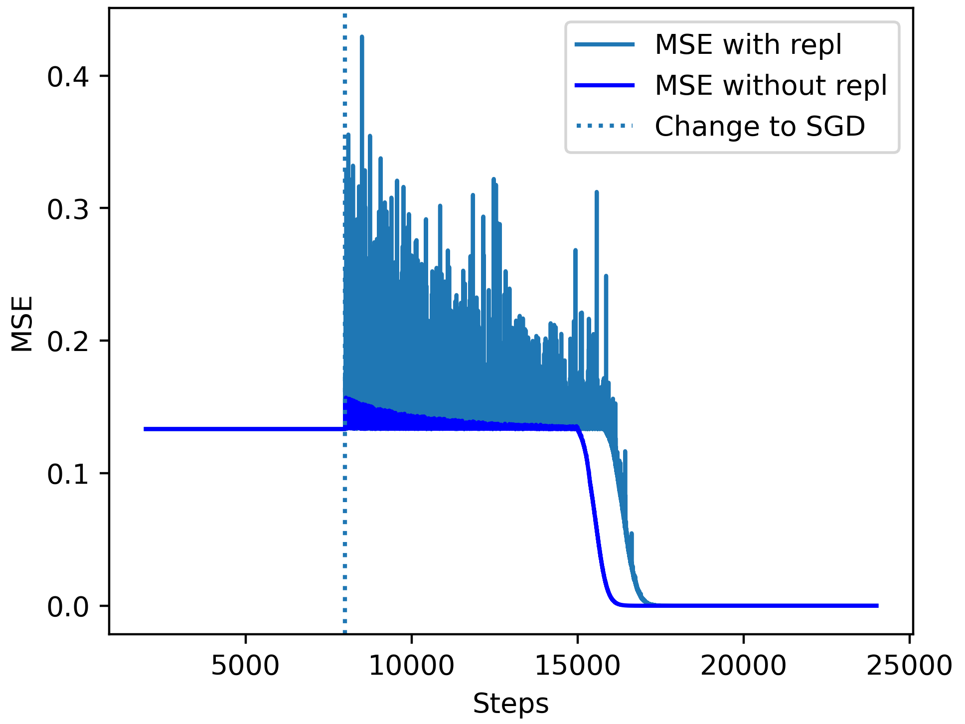
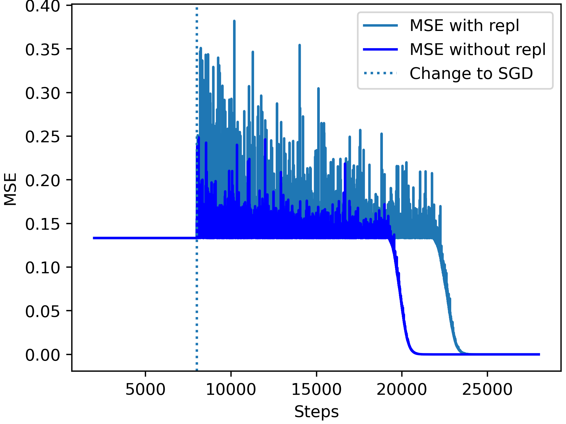
Figure 5: This is in the setting of Fig. 4. We compare on the left SGDs with lower batchsize ($b=1$) and on the right SGD with bigger batchsize ($b=2$).
We see here the SGD without replacement escapes local minima in which GD converges (by traveling flat areas) faster that SGD with replacement and with much smaller oscillations as it shows smaller variance. They both converge to a global minimum.

8.2 Towards Low (Weighted-)Variance

The regularizer we found in Theorem 3 penalizes the noise variance, through the lens of the matrix $S$:

$$\text{Regularizer}=\mathbb{E}\left[(\nabla L(z)-\nabla L)^{\top}S\,(\nabla L(z)-\nabla L)\right].$$

Thus explicitly biasing the dynamics in areas where the noise variance is smaller. This implies that SGD without replacement not only has a smaller variance than SGD with replacement, but it biases the dynamics in areas where the variance of later steps is even smaller. This may be also the case of SGD with replacement, [Li et al., 2022, Chen et al., 2023], although due to a different effect known in the statistical physics community as thermophoresis and studied in diverse communities of mathematicians, see Fokker-Plank equations.

8.3 The Bias of SGD with replacement

[Damian et al., 2021] showed that also SGD with replacement has a bias, i.e., the deviation between trajectories of SGD with replacement and GD is non-zero. However, to find a term whose expectation is different from its full-batch version one has to look deeper into Taylor. Precisely, into terms of the kind

$$\eta\nabla^{3}L(B_{i})[\eta\nabla L(B_{j})]^{2},\qquad i>j.$$

These terms fall into the approximation error correction of the bias of SGD without replacement, so, in particular, the bias effect of SGD with replacement is realistically orders of magnitude smaller.

Proposition 10 (Adaption of Proposition 5, [Damian et al., 2021]).

Let $\theta^{*}$ be any global minimizer of $L$. Let $R$ satisfy

$$R=(I-\eta\nabla^{2}L(\theta^{*}))R(I-\eta\nabla^{2}L(\theta^{*}))+\eta\lambda\operatorname{Cov}(\nabla L(\theta^{*})).$$

Then the vector field of the expected direction of our steps is

$$\hat{\nabla}L\approx\nabla\left[L+\lambda\langle\nabla^{2}L(\theta),R\rangle\right]$$

with $\lambda$ constant dependent on the learning rate. Thus, SGD with replacement minimizes the quantity $\langle\nabla^{2}L(\theta),R(\vartheta)\rangle$ (here you do not differentiate the $R$, only the $\nabla^{2}L(\theta)$), within the manifold in which the loss $L$ is minimized.

9 Broad Applicability and Limitations

The primary objective of this section is understanding technically how our work compares to other studies and to what extent the following question has been answered.

Question:
Can we characterize the minima to which SGD converges? How?

We argue that from a certain point of view, we employ the minimal and most natural set of assumptions for such an analysis. We discuss the broad applicability of this approach in §9.1. We discuss the limitations of our findings in §9.2.

9.1 Generality and Optimality of our Approach

As previously discussed in §2.3, there are several reasons for conducting a local analysis. This is primarily due to the inapplicability of "global" methods such as stochastic approximation by Robbins and Monro. Also, there is a lack of understanding of the geometry of the manifolds. Essentially, conducting a local analysis means expanding in the Taylor series or a similar approximation technique. In this context, as explained in Section 2.4, a Taylor expansion over the $k$ steps of an epoch can be represented as a sum of product of terms of the form:

$$\text{coefficient}\ \cdot\ \eta\ \cdot\ k\ \cdot\ \text{function}\big{(}\nabla^{i}L(\cdot,\cdot)\big{)}$$

for some $i\in\mathbb{N}$, some real coefficient, and a function that could be, e.g., an average over batches, and so on. For such Taylor expansions to converge and represent our trajectory, it is thus necessary that some of the terms above are small. As argued in Section 2.4, $\eta k\nabla L$ appears in every term and it is the only such term that vanishes throughout the training. This happens because $\eta$ is annealed and $\nabla L$ converges to 0 approaching a stationary point. Moreover, no matter the size of the other derivatives, if $\eta k\nabla L\ll 1$ the series generally converges. Consequently, for the Taylor series to converge, or analogously for a local analysis to be performed, requiring the assumption $\eta\nabla L\ll 1$ is the most natural of the possible necessary conditions. An analysis based solely on this assumption is thus highly versatile, arguably the broadest in scope among local analyses.

Whenever one can use a local argument, one can expand in Taylor, in particular, generally $\eta^{>1}\cdot k\cdot\nabla L\ll 1$. Thus our analysis characterizes the dynamics.

Our approach differs from past community efforts that relied on stricter assumptions $\eta k\ll 1$ [Smith et al., 2021, Roberts, 2021], or conditions involving other higher order derivatives. The only works that could relax these assumptions usually assume independence between single steps, e.g. [Damian et al., 2021]. We demonstrated that the inherent effect of SGD without replacement is due to the dependence. This means that that such results, while being still instrumental in addressing the effect of other algorithms, do not apply to our setting.

9.2 Limitations: Broader Scope implies Weaker Results

In the context of small learning rate [Smith et al., 2021, Roberts, 2021] or independent steps [Damian et al., 2021, Li et al., 2022] the results are mathematically elegant: we have a penalized loss on which GF or GD mirrors the trajectory of the SGD. Those works deliver insightful heuristics and theorems about where the trajectory leads and the generalization improvements. In our context, however, as discussed in §2, with $\eta\not\!\ll 1$ and dependent steps, we cannot explain convergence using those results and techniques. This limitation hampers our ability to establish the beautiful convergence results that mark the earlier studies. We will investigate this in future works, however, the absence of such strong convergence results would not be entirely surprising. It would align with the understanding that in many contexts there is not such a thing as a potential that the algorithms are minimizing. This has been shown for instance for gradient flow for ReLU networks by [Vardi and Shamir, 2021]. It has also been discovered by [Damian et al., 2021] and later made rigorous by [Li et al., 2022] for the case of SGD, in which it is possible that SGD cycles. We can thus only hope to better characterize the trajectories. This is exactly what we manage to do with our technique.

Our Theorem 2 characterizes the path-dependent regularizer of the algorithm in analysis. In general, we were unable to describe our results, unlike previous work, as "SGD without replacement works as a specific (different) optimization algorithm on a modified loss". This, however, may not be a shortcoming of our analysis. Rather, it could underscore the nature of the effect, which proves more challenging to describe mathematically than many earlier hypotheses. That said, heuristically the meaning of Theorem 2 is similar to working with a penalized loss: If the regularizer is not minimized it guides the trajectory towards areas where it decreases. Returning to the main question of this section, we could not precisely define the minima to which SGD converges, in contrast to previous studies that have achieved such a goal in different contexts. However, the task is likely unattainable in full generality. Identifying such specific cases where this is possible is beyond the scope of our current work.

10 Conclusions

Conclusion.

We showed that SGD without replacement implicitly regularizes by biasing the dynamics towards areas with lower variance. This is due to the dependence of the steps and manifests as a drift-like effect, not attributable to diffusion or a Fokker-Planck-like argument. We demonstrate that this leads to a form of regularization, enabling the algorithm to navigate through flat areas more quickly and with fewer oscillations than expected.

Future directions

Our work, between others [Damian et al., 2021], highlights the critical need to focus on understanding the geometry of the optimization landscape in machine learning. The regularizer we identified is highly dependent on the geometry of the landscape. It has become clear that the landscape’s shape, particularly its curvature and higher-order derivatives, plays a more significant role than previously thought. This goes beyond just the noise within Stochastic Gradient Descent (SGD) or the effect of discretization. The way these geometrical aspects interact with algorithms like SGD leads to unique trajectories and convergence behaviors.

Moving forward, we should explore how these geometrical features influence optimization, especially in non-linear models like neural networks, and induce the unexpected phenomena we see in learning. Understanding the interplay between the landscape’s curvature and geometry in non-convex settings and algorithmic behavior is key. This approach promises to unveil deeper insights into the optimization process, and thus into what properties the neural networks used in practice have. Also, this article is about point-wise regularization effect throughout the trajectory. The regularization effect that we unveil is path-dependent. In the future, we need to investigate what this implies on the convergence.

Appendix A The Variance of SGD without replacement

A.1 What we Know

[Mishchenko et al., 2020] computed the variance of one step of SGD without replacement. They showed that starting from the minimum of a strong convex objective function, the variance of one step of SGD is upper bounded by $O(\eta c\nabla^{2}L)$, while for SGD with replacement, it is upper bounded by $O\left(\eta\frac{\lambda_{max}\nabla^{2}L}{\lambda_{min}\nabla^{2}L}\right)$. They also observed empirically that SGD without replacement in some strong convex settings has higher variance at initialization. However, they noted that the variance for SGD without replacement decreases more rapidly. After approximately $O(1)$ epochs, its variance becomes lower than that of SGD with replacement, leading to faster convergence. They also have a result for non-convex scenarios; yet, it applies in the regime where $c\lambda_{max}\nabla^{2}L<1/\sqrt{2b}$, which may be too restrictive for practical applications.

Nevertheless, these findings alone help explain the smaller variance sizes observed in certain settings. In some cases indeed, as the dynamics converge, it gets trapped in invariant sets like those identified by [Chen et al., 2023]. Within these invariant sets, the dynamics might exhibit local strong convexity. This is the case for diagonal networks, for example, but typically not for general neural networks [Liu et al., 2020]. [Liu et al., 2020]. For instance, consider the toy model $(a\cdot bx-y)^{2}$, where $a,b,x,y\in\mathbb{R}^{+}$, of §B. In this model, the dynamics are driven to the hyperplane where $a=b$, either by the regularizer in SGD without replacement or by diffusion in SGD with replacement, and get trapped there. When restricted to the subspace $a=b$, the objective function becomes locally strongly convex, specifically $(a^{2}x-y)^{2}$. If $x,y>0$, near the minimum at $a=\sqrt{y}/\sqrt{x}$, oscillations are observed to be of size $O(\eta^{2})$ for SGD without replacement, compared to $O(\eta)$ for SGD with replacement.

Nevertheless, in practical scenarios where the Hessian has large or zero eigenvalues, these worst-case results from convex optimization may not fully explain the trajectory or the size of the variance.

A.2 When the Variance is Smaller

It is easy to see that in the regime in which $c\|\nabla^{2}L\|\ll 1$ the update to the parameters resulting from an epoch of SGD without replacement is approximately deterministic; indeed,

$$\theta^{SGD}_{k}-\theta\quad=\quad-\eta\sum_{i=1}^{k}\nabla L(B_{i})\ +\ O(c\|\nabla^{2}L\|)\quad=\quad-c\nabla L\ +\ O(c\|\nabla^{2}L\|).$$

This suggests already that: (i) We have a big variance only in the presence of big eigenvalues of the Hessian, and in case only in the direction of the eigenvectors of the big eigenvalues. And (ii) we can expect the variance of SGD without replacement to be smaller than the one of SGD with replacement when some of the key ingredients of the trajectory are small.

Moreover, in the case in which our discretization explains the trajectory, i.e., $\eta\nabla L\ll 1$, the variance of SGD without replacement get shrunk by the addition of the regularizer in the term $-\mathbb{E}\left[\begin{subarray}{c}\text{trajectory}\\ \text{without replacement}\end{subarray}\right]^{2}$.

We can thus conclude that the variance of the noise in one epoch of SGD without replacement is smaller than the one with replacement at least when (i) the Hessian $c\nabla^{2}L\ll 1$ is small, or (ii) the gradients $c\nabla L\ll 1$ are small. And we can go even further, consider at any epoch of SGD the update in the direction of the eigenvector $v_{\lambda}$ of the eigenvalue $\lambda$ of the Hessian.

• If $c\lambda\ll 1$, $\langle v_{\lambda},\nabla L\rangle\neq 0$, the eigenvalue is part of the bulk of small ones, then SGD without replacement has very small variance in that direction, unlike SGD with replacement. The push in that direction, in first approximation, is due only to full-batch gradient descent and the regularizer.

• For all $\lambda$s, even the big ones, if $\langle v_{\lambda},\nabla L\rangle\ll 1$, then SGD without replacement has a small variance in that direction, in particular, smaller than SGD with replacement. The push in that direction, in first approximation, is due only to the regularizer, and if $\eta\lambda>1$ to the oscillation of GD.

Appendix B Practical Example: the Setting for the Plots

The setting of Figs. 1 and 2 is the easiest possible neural network setting trainable with SGD. We have the $f(\theta,x)=\theta_{1}\cdot\theta_{2}\cdot x$, it is a linear shallow network with width, input, and output dimensions being 1. The Dataset consists of 3 points $D=\{(1,1),(1,2),(1,0)\}$, the chosen loss is the MSE. Precisely, the loss $L(\theta)=(\theta_{1}\cdot\theta_{2}-1)^{2}+(\theta_{1}\cdot\theta_{2}-2)^{2}+(\theta_{1}\cdot\theta_{2})^{2}$ with initialization the white bullet $\theta=(1,6)$. The lowest norm global minimum is $\pm(1,1)$.

This setting shares the same peculiarities of linear diagonal network scenarios. In particular, our experiments extends to bigger linear diagonal networks. Precisely, we have that, (i) the minimum with the widest valley is also the min-norm solution, (ii) the min-norm solution coincindes also with the global minimum that zeros out our regularizer, and (iii) the global minima have loss $>0$. The datapoints have the same $x$ but different $y$. Thus the SGD noise never fades out and keeps pushing toward the direction of the regularizer. Moreover, this makes SGD with replacement coincide with a version of GD with label noise. This is not a bad thing as label noise has generally better and understood generalization capabilities [Damian et al., 2021].

The code that generated the figures can be found on this github repository.

Appendix C The Effect of Mini-batching

The goal of this section is to understand the role of the following two properties of SGD without replacement:

• The fact that the mini-batches add up to the dataset.

• The fact that once the mini batches are sampled we do not care about their order.

The first property above is shared by the SGD without replacement and Shuffle Once, and the second by SGD with and without replacement. However, once we take the expectation over the possible outcome of the initial shuffling, the same holds for Shuffle Once. We argue that it is the fact that we do not care about the order that allows us to rewrite our quantity as a derivative of a penalization. This properties are not shared, e.g., by Adam.

C.1 Fixed Batches SGD Trajectory

We address here the following question:

Question:
Assume we sampled already the batches $B_{1},B_{2},\ldots,B_{k}$ (fixed) and we make $k$ steps of SGD using them. How far are we from the GD trajectory?

For the reasons described in §2.3 and §2.4, we expand $k$ steps of SGD and GD with learning rate $\eta$ at the beginning of the epoch, and we keep the terms in which $\nabla L(\cdot)$ appears to the power 1. We write the difference between this quantity in the case of SGD and the case of GD and we obtain the following

Proposition 11.

The deviation due to mini-batches from the trajectory of the GD is

$$\begin{split}\eta^{2}\sum_{1\leq i<j\leq k}\nabla^{2}L(B_{j})\Bigg{[}\prod_{h=i+1}^{j-1}[I-\eta\nabla^{2}L(B_{h})]\Bigg{]}\ \nabla L(B_{i})\quad-\quad\begin{subarray}{c}\text{same but full-batch:}\\ B_{j}\curvearrowleft D\text{ for all }j\leq epoch\end{subarray}.\end{split}$$

up to first order in $\eta k\nabla L(B_{i})$, $i=1,2,\ldots,k$. The error is of order $O(\eta^{2+}k^{3}\|\nabla L\|^{2}).$

More details about the computation are in the proof in Appendix F, more details about the size of the error in §J.

C.2 The Implicit Bias of the Order

We derived a formula for the deviation in the trajectory, which depends on the order in which we observe the batches. It makes thus sense to examine the expectation and standard deviation of this SGD discretization with respect to the GD trajectory due to the randomly uniform order of the batches.

Assume we sampled already the batches $B_{1},B_{2},\ldots,B_{k}$ (fixed). How far do we go from the GD/GF trajectory, on average over the possible orders of the batches?

To do it, we consider the following quantity

$$\frac{\eta^{2}}{2}\nabla_{\theta}\sum_{1\leq i<j\leq k}[\nabla^{\color[rgb]{1,0,0}1}L(B_{j})]^{\top}\Bigg{[}\prod_{h=i+1}^{j-1}[I-\eta\nabla^{2}L(B_{h})]\Bigg{]}\ \nabla L(B_{i})$$ (11)

The derivative of this quantity in $\theta$ is

$$\begin{split}&\quad\frac{\eta^{2}}{2}\sum_{1\leq i<j\leq k}\nabla^{2}L(B_{j})\ \Bigg{[}\prod_{h=i+1}^{j-1}[I-\eta\nabla^{2}L(B_{h})]\Bigg{]}\ \nabla L(B_{i})\qquad\leftarrow\text{\lx@cref{creftype~refnum}{theo:SGD_effect_fixed_batches}!}\\ &+\frac{\eta^{2}}{2}\sum_{1\leq i<j\leq k}\nabla^{2}L(B_{i})\ \Bigg{[}\prod_{h=i+1}^{j-1}[I-\eta\nabla^{2}L(B_{h})]\Bigg{]}^{\top}\ \nabla L(B_{j})\qquad\ \ \leftarrow\text{flipped }i,j\\ &+\frac{\eta^{2}}{2}\sum_{1\leq i<j\leq k}\nabla L(B_{j})^{\top}\ \Bigg{[}\nabla_{\theta}\prod_{h=i+1}^{j-1}[I-\eta\nabla^{2}L(B_{h})]\Bigg{]}^{\top}\ \nabla L(B_{i}).\ \ \leftarrow\text{error term!}\end{split}$$ (12)

In the first line we have half of the term in 9, and in the second line we have the same quantity but with the indices switched. The third line is a part of the error as constitute a term of second order in $\eta\nabla L$. This is the key idea of the proof of the following theorem other than of the main theorem, Theorem 2.

Proposition 12.

With an additive error of size smaller than $O(\text{that})\cdot(\eta k\nabla L+1/k)$, we have

$$\theta_{k}^{SGD}\quad\overset{\begin{subarray}{c}\text{expectation over}\\ \text{order of batches}\end{subarray}}{=}\quad\theta_{k}^{GD}\quad-\quad\eta\nabla_{\theta}Regularizer$$

where where the regularizer is

$$\begin{split}\eta\mathbb{E}_{order}\left[\sum_{1\leq i<j\leq k}\nabla L(B_{j})^{\top}\Bigg{[}\prod_{h=i+1}^{j-1}[I-\eta\nabla^{2}L(B_{h})]\Bigg{]}\ \nabla L(B_{i})\right]\quad-\quad\begin{subarray}{c}\text{same but full-batch:}\\ B_{j}\curvearrowleft D\text{ for all }j\leq epoch\end{subarray}.\end{split}$$

We can thus conclude that: (i) The reason why we can rewrite this deviation as the derivative of a potential is that we do not care about the order in which we see the batches. And (ii) this happens for every SGD technique once we sample the batches, irrespective of how we sampled them.

Appendix D The Philosophy of the Analysis

We briefly present here the philosophy and tools of our analysis and proof.

Our analysis consists of two main phases: (i) writing down the low-order part of the deviation, noticing that it is the derivative of a quantity, and (ii) computing its moments. Precisely, we start by expanding in Taylor at the beginning of the epoch the shift in trajectory between the SGD of learning rate $\eta$ with batches $B_{1},B_{2},\ldots,B_{k}$ and the GD or learning rate $\eta\cdot k$. We do this by iteratively considering the shift after $i$ steps with the GD with learning rate $\eta\cdot i$ on $\cup_{j=1}^{i}B_{j}$. Indeed, we find that at every step $i$ the shift gets multiplied by $I-\eta\nabla^{2}L(B_{i})$ and we add the terms $\eta^{2}\nabla^{2}L(B_{i})\sum_{i<j}\nabla L(B_{j})$ (this will become the regularizer) and the higher-order terms of the Taylor will become the error. The part highlighted is the leading part in the case in which $\eta\nabla L(B_{1}),\eta\nabla L(B_{1})+\eta\nabla L(B_{2})),\ldots,\eta\sum_{j=1}^{k}\nabla L(B_{j})$ are small. Indeed those quantities appear with exponent 1 in the "regularizer" part and with exponent $\geq 2$ in the part that we consider to be the error. It is important to notice that later we will weaken these assumptions. Precisely, if we take the expectation already of the Taylor expansion of the error and then we highlight this part, and not vice-versa, we will be able to just assume that the expectations are small. This will imply that the result works in the case in which $\eta^{1+}k\nabla L\ll 1$.

We follow by noticing that by adding terms that are $O(\eta k\nabla L)^{2}$, that thus fall into the error part, this deviation between the trajectories coincides with the derivative of a quantity. Now by subtracting to what we obtained the analogous term but in the setting in which $B_{i}=D$ for all $i$, i.e., the shift between small step and big step GD, we obtain our regularizer (still as a function of the batches, there are still no expectations involved).

We will later conclude by computing the moments of these quantities arising from the Taylor series in the setting without replacement. In this setting, we develop a lemma that helps us compute the moments of the quantities in play. More details about this in §E.

Appendix E Dealing with Expectations

To prove our main result, we need to be able to compute all the expectations that we encounter. Those are taken over the SGD sampling procedure, i.e., sampling without replacement:

Setting 13 (Sampling without replacement).

Assume $z_{1},z_{2},\ldots,z_{k}$ are sampled in one of the following two equivalent ways.

1. $\{z_{1},z_{2},\ldots,z_{k}\}$ is a set of $k$ different elements that has been uniformly sampled from the family of all the possible different subsets (without multiple copies) of cardinality $k$ of a set $D$ with cardinality $n$.

2. We sampled $z_{1}$ uniformly from $D$, $z_{2}$ uniformly from $D\backslash\{z_{1}\}$, $\ldots$, and $z_{k}$ uniformly from $D\backslash\{z_{1},z_{2},\ldots,z_{k-1}\}$.

All the expectations in what follows will be over this sampling procedure. Indeed, if we see a batch or a data point we will not see it until the end of the epoch.

We will assume we have a sequence of functions that take in input elements of $D$ and output a tensor such that the shapes of the tensors match and we can make a product. Precisely, for all $i\in\{1,2,\ldots,k\}$ we have $f_{i}\colon D\to\mathbb{R}^{n_{i}\times n_{i+1}}$ where $n_{1},n_{2},\ldots,n_{k+1}\in\mathbb{N}$. Precisely, in the following these $f$s will take a training data point $z\in D$ in input and they will output a derivative of the loss in the parameters evaluated at that data point, e.g. $f_{1}(z_{1})=I-\nabla_{\theta}^{2}L(\theta,z_{1})$.

E.1 Lemma for Expectations Without Replacement

Lemma 14.

Let $D=\{z_{j}\}_{j\in\{1,2,\ldots,n\}}\subseteq\mathbb{R}^{d}$, let $B_{1},B_{2},\ldots,B_{k}$ batches of size $b$ sampled without replacement from $D$, see 13. Let $A\in\mathbb{R}^{d\times d}$ and denote by $Z_{i}:=\tfrac{1}{b}\sum_{z\in B_{i}}z$ the average of the vectors in the $i-th$ batch, by $\bar{z}:=\frac{1}{n}\sum_{z\in D}z$. Then

$$\mathbb{E}_{\left[\begin{subarray}{c}without\\ replacement\end{subarray}\right]}\left[\sum_{i=1,j}^{h}Z_{i}^{\top}AZ_{j}\right]-h\bar{z}^{\top}A\bar{z}\quad=\quad\frac{h(n-hb)}{b(n-1)}\left(\mathbb{E}_{z\in D}\big{[}z^{\top}Az\big{]}-\bar{z}^{\top}A\bar{z}\right).$$

Proof.

Denote by $\alpha:=\mathbb{E}_{z\in D}z^{\top}Az-\bar{z}^{\top}A\bar{z}$. Note that

$$\mathbb{E}_{\left[\begin{subarray}{c}without\\ replacement\end{subarray}\right]}\left[\sum_{i,j=1}^{h}Z_{i}^{\top}AZ_{j}\right]\quad=\quad\mathbb{E}_{\left[\begin{subarray}{c}without\\ replacement\end{subarray}\right]}\left[\sum_{1\leq i\neq j\leq h}Z_{i}^{\top}AZ_{j}+\sum_{1\leq i\leq h}Z_{i}^{\top}AZ_{i}\right]$$

$$\begin{split}&h(h-1)\left(-\frac{\alpha}{n-1}\right)+h\left(\frac{b-1}{b}\bar{z}^{\top}A\bar{z}-\frac{b-1}{b}\frac{\alpha}{n-1}+\frac{1}{b}\mathbb{E}_{z\in D}[z^{\top}Az]\right)\\ &=\quad h\bar{z}^{\top}A\bar{z}-\frac{1}{n-1}\left(h^{2}-\frac{h}{b}\right)\alpha+\frac{h}{b}\alpha\\ &=\quad h\bar{z}^{\top}A\bar{z}-\frac{h^{2}b-hn}{b(n-1)}\alpha.\end{split}$$ (13)

∎

E.2 The Main Lemma

Lemma 15 (How the expectation looks like).

Assume we are in 13 above. Then, when $S$ is sampled as in Item 1 of 13, the expectation $\mathbb{E}\left[f_{1}(z_{1})\cdot f_{2}(z_{2})\cdot\ldots\cdot f_{k}(z_{k})\right]$, is equal to

$$\begin{split}\left[\prod_{i=0}^{k-1}(n-i)\right]^{-1}\sum\prod_{i=1}^{k}f_{i}(z_{i})\end{split}$$ (14)

where, thus, the sum is taken over all the possible $k$-uple $(z_{1},z_{2},\ldots,z_{k})$ of $k$ different elements of $D$. By averaging over the sampling technique in Item 2, we obtain quantities like the following in the case of commutation of the $f_{i}$s.

$$\begin{split}\left[\prod_{i=0}^{k-1}\frac{n}{n-i}\right]\sum_{j=1}^{k}\sum_{\sigma\in\Pi}\prod_{\begin{subarray}{c}\text{all the possible}\\ 0=i_{0}<i_{1}<\ldots<i_{j}=k\end{subarray}}\!\!\!\!\!\left[\frac{-1}{n}\right]^{i_{j}-i_{j-1}-1}\mathbb{E}_{z\in D}\left[\prod_{h=i_{j-1}+1}^{i_{j}}f_{\sigma(h)}(z)\right].\end{split}$$ (15)

where $\Pi$ is the set of all the possible permutations of $\{1,2,\ldots,k\}$. That is the sum of all the possible products of expectations of products of functions. Each of the expectations of products of $l$ functions is multiplied by $\left[\frac{-1}{n}\right]^{l-1}$. Another way to rewrite it is $\left[\prod_{i=0}^{k}\frac{n}{n-i}\right]$ multiplied by

$$\begin{split}&\prod_{i=1}^{k}\mathbb{E}[f_{i}]-n^{-1}\sum_{i\neq j}\mathbb{E}[f_{i}f_{j}]\prod_{m\neq j,i}\mathbb{E}[f_{m}]+n^{-2}\sum_{i\neq j\neq h\neq l}\mathbb{E}[f_{i}f_{j}]\mathbb{E}[f_{h}f_{l}]\prod_{m\neq j,i,h,l}\mathbb{E}[f_{m}]+\ldots\end{split}$$ (16)

Proof of Lemma 15..

Let us now prove what above, regarding the first part in Eq. 14, it follows directly from the definition of average. We prove the other thing by induction. Note that for $k=1,2$ we have the result in Eq. 15 already (base case). Indeed, note that

$$\mathbb{E}_{D\backslash\{z\}}[f]\quad=\quad\frac{1}{n-1}\sum_{x\in D\backslash\{z\}}f(x)\quad=\quad\frac{n}{n-1}\left[\mathbb{E}_{D}[f]-\frac{f(z)}{n}\right]$$ (17)

and by plugging this in

$$\begin{split}\mathbb{E}_{z_{1}\in D}[f_{1}(z_{1})\cdot\mathbb{E}_{z_{2}\in D\backslash\{z_{1}\}}[f_{2}(z_{2})]]\quad&=\quad\frac{n}{n-1}\mathbb{E}_{D}[f_{2}]\mathbb{E}[f_{1}]-\frac{1}{n-1}\mathbb{E}_{D}\left[f_{1}f_{2}\right].\end{split}$$ (18)

Let us see the step $k=3$ to better explain what is happening

$$\begin{split}&\mathbb{E}_{z_{1}\in D}[f_{1}(z_{1})\cdot\mathbb{E}_{z_{2}\neq z_{3}\in D\backslash\{z_{1}\}}[f_{2}(z_{2})f_{3}(z_{3})]]\\ &\quad=\quad\mathbb{E}_{z_{1}\in D}\left[f_{1}(z_{1})\cdot\left(\frac{n-1}{n-2}\mathbb{E}_{D\backslash\{z_{1}\}}[f_{2}]\mathbb{E}_{D\backslash\{z_{1}\}}[f_{3}]-\frac{1}{n-2}\mathbb{E}_{D\backslash\{z_{1}\}}\left[f_{2}f_{3}\right]\right)\right]\\ &\quad=\quad\mathbb{E}_{z_{1}\in D}\Bigg{[}f_{1}(z_{1})\cdot\bigg{(}\frac{n-1}{n-2}\frac{n}{n-1}\left[\mathbb{E}_{D}[f_{2}]-\frac{f_{2}(z_{1})}{n}\right]\frac{n}{n-1}\left[\mathbb{E}_{D}[f_{3}]-\frac{f_{3}(z_{1})}{n}\right]\\ &\qquad-\frac{1}{n-2}\left[\frac{n}{n-1}\mathbb{E}_{D}\left[f_{2}f_{3}\right]-\frac{f_{2}(z_{1})f_{3}(z_{1})}{n-1}\right]\bigg{)}\Bigg{]}.\end{split}$$ (19)

Next by noting that

$$\begin{split}(n-1)\ \frac{f_{2}(z_{1})}{n-1}\frac{f_{3}(z_{1})}{n-1}\quad=\quad\frac{f_{2}(z_{1})f_{3}(z_{1})}{n-1}\end{split}$$ (20)

we conclude that

$$\begin{split}&\mathbb{E}_{z_{1}\neq z_{2}\neq z_{3}\in D}[f_{1}(z_{1})f_{2}(z_{2})f_{3}(z_{3})]\quad=\quad\frac{n^{3}}{n(n-1)(n-2)}\mathbb{E}[f_{1}]\mathbb{E}[f_{2}]\mathbb{E}[f_{3}]\\ &\quad-\frac{n^{2}}{n(n-1)(n-2)}\left(\mathbb{E}\left[f_{1}f_{2}\right]\mathbb{E}[f_{3}]+\mathbb{E}[f_{1}]\mathbb{E}\left[f_{2}f_{3}\right]+\mathbb{E}\left[f_{1}\cdot\mathbb{E}[f_{2}]\cdot f_{3}\right]\right)\\ &\quad+2\frac{n}{n(n-1)(n-2)}\mathbb{E}[f_{1}f_{2}f_{3}].\end{split}$$ (21)

More generally we will have all the possible products showing up with the multiplier $(-n)^{-order+1}$. Indeed or what regards the inductive step, note that by tower rule

$$\begin{split}\mathbb{E}_{D}\left[\,f_{1}(z_{1})\cdot f_{2}(z_{2})\cdot\ldots\cdot f_{k}(z_{k})\right]\quad=\quad\mathbb{E}_{z_{1}\in D}\left[f_{1}(z_{1})\ \cdot\ \mathbb{E}_{D\backslash\{z_{1}\}}\left[f_{2}(z_{2})\cdot\ldots\cdot f_{k}(z_{k})\right]\right]\end{split}$$ (22)

So the expectation for $z_{1},z_{2},\ldots,z_{k}\in D$ without replacement it is the same as the expectation over $z_{1}\in D$ of the expectation for $z_{2},z_{3},\ldots,z_{k}\in D\backslash\{z_{1}\}$ without replacement. We will also prove that Now, applying the inductive hypothesis for $k\curvearrowleft k-1$ and $D\curvearrowleft D\backslash\{z\}$ on $\mathbb{E}_{D\backslash\{z_{1}\}}\left[f_{2}(z_{2})\cdot\ldots\cdot f_{k}(z_{k})\right]$ we obtain that

• The multiplier is $\prod_{i=0}^{k-1}\frac{n}{n-i}$.

• That we have $n^{k}\prod_{i=1}^{k}\mathbb{E}[f_{i}]-n^{k-1}\sum_{i<j}\mathbb{E}[f_{i}f_{j}]\prod_{h\neq i,j}\mathbb{E}[f_{h}]+\ldots$ and in general appears every possible combination of expectations of products of the functions, such that when we are taking the expectations of $l$ functions together, we have $(-1/n)^{l-1}$ multiplying the head coefficient.

Remark 16.

From now on we perform the computations in the case of commutations, but they would not change at all in case of no commutation. It is just more difficult

Let us assume it works for $D\backslash\{z_{1}\}$ and $k-1$. Then the expectation in that setting is the following and satisfies the points above.

$$\begin{split}\left[\prod_{i=1}^{k}\frac{n-1}{n-i}\right]\left[\prod_{i=2}^{k}\mathbb{E}_{D\backslash\{z_{1}\}}[f_{i}]-(n-1)^{-1}\sum_{i\neq j}\mathbb{E}_{D\backslash\{z_{1}\}}[f_{i}f_{j}]\prod_{m\neq i,j}\mathbb{E}_{D\backslash\{z_{1}\}}[f_{m}]+\ \ldots\ \right]\end{split}$$ (23)

Thus plugging this into Eq. 22 we obtain that $\mathbb{E}_{D}\left[\,f_{1}(z_{1})\cdot f_{2}(z_{2})\cdot\ldots\cdot f_{k}(z_{k})\right]$ is equal to

$$\begin{split}\mathbb{E}_{D}\Bigg{[}f_{1}(z_{1})\cdot\Bigg{[}(n-1)^{k-1}\prod_{i=2}^{k}\mathbb{E}_{D\backslash\{z_{1}\}}[f_{i}]-(n-1)^{k-2}\sum_{i\neq j}\mathbb{E}_{D\backslash\{z_{1}\}}[f_{i}f_{j}]\prod_{m\neq i,j}\mathbb{E}_{D\backslash\{z_{1}\}}[f_{m}]\Bigg{]}\Bigg{]}\end{split}$$ (24)

multiplied by $\left[\prod_{i=1}^{k}\frac{1}{n-i}\right]$. Next, note that

$$\mathbb{E}_{D\backslash\{z\}}[f]\quad=\quad\frac{1}{n-1}\sum_{x\in D\backslash\{z\}}f(x)\quad=\quad\frac{n}{n-1}\left[\mathbb{E}_{D}[f]-\frac{f(z)}{n}\right].$$ (25)

Applying this above, we obtain

$$\begin{split}&\left[\prod_{i=1}^{k}\frac{1}{n-i}\right]\mathbb{E}_{D}\Bigg{[}f_{1}(z_{1})\cdot\Bigg{[}(n-1)^{k-1}\prod_{i=2}^{k}\frac{n}{n-1}\Bigg{[}\mathbb{E}[f_{i}]-\frac{f_{i}(z_{1})}{n}\Bigg{]}\\ &\quad-(n-1)^{k-2}\sum_{2\leq i\leq j\leq k}\frac{n}{n-1}\left[\mathbb{E}[f_{i}f_{j}]-\frac{f_{i}(z_{1})f_{j}(z_{1})}{n}\right]\prod_{n\neq i,j,1}\frac{n}{n-1}\left[\mathbb{E}[f_{i}]-\frac{f_{i}(z_{1})}{n}\right]\Bigg{]}\Bigg{]}\\ &=\left[\prod_{i=0}^{k}\frac{1}{n-i}\right]\mathbb{E}_{D}\Bigg{[}f_{1}(z_{1})\cdot\Bigg{[}n^{k-1}\prod_{i=2}^{k}\Bigg{[}\mathbb{E}[f_{i}]-\frac{f_{i}(z_{1})}{n}\Bigg{]}\\ &\qquad\qquad\quad\qquad\qquad-n^{k-2}\sum_{2\leq i\leq j\leq k}\left[\mathbb{E}[f_{i}f_{j}]-\frac{f_{i}(z_{1})f_{j}(z_{1})}{n}\right]\prod_{h\neq i,j,1}\left[\mathbb{E}[f_{h}]-\frac{f_{h}(z_{1})}{n}\right]\Bigg{]}\Bigg{]}\end{split}$$ (26)

where the average is now taken over $D$. Note that for all $i,j$ it holds

$$\begin{split}n^{k-1}\ \frac{f_{i}(z_{1})}{n}\frac{f_{j}(z_{1})}{n}\prod_{h\neq i,j,1}^{k}\mathbb{E}[f_{h}]\quad=\quad n^{k-2}\ \frac{f_{i}(z_{1})f_{j}(z_{1})}{n}\prod_{h\neq i,j,1}^{k}\mathbb{E}[f_{h}]\end{split}$$ (27)

and the same holds for all the other expectations of products of more functions. In general, the sign and power of $n$ multiplying all the expectations of products of $l$ terms is $n^{-l+1}$. Precisely, we obtain

$$\begin{split}&\mathbb{E}\left[f_{1}(z_{1})\cdot f_{2}(z_{2})\cdot\ldots\cdot f_{k}(z_{k})\right]\\ &\qquad=\left[\prod_{i=0}^{k}\frac{1}{n-i}\right]\mathbb{E}_{D}\Bigg{[}f_{1}(z_{1})\cdot n^{k}\Bigg{[}\prod_{j>1}\mathbb{E}[f_{j}]-\sum_{i=2}^{k}\frac{f_{i}(z_{1})}{n}\prod_{j\neq 1,i}\mathbb{E}[f_{j}]\\ &\qquad\qquad\qquad-n^{k-1}\sum_{2\leq i<j}\Bigg{[}\mathbb{E}[f_{i}f_{j}]\prod_{n\neq i,j,1}\left[\mathbb{E}[f_{i}]-\frac{f_{i}(z_{1})}{n}\right]\Bigg{]}\ +\ \ldots\Bigg{]}\end{split}$$ (28)

That is equal to the usual $\left[\prod_{i=0}^{k}\frac{1}{n-i}\right]$ multiplied by

$$\begin{split}&n^{k}\prod_{i=1}^{k}\mathbb{E}[f_{i}]-n^{k-1}\sum_{i\neq j}\mathbb{E}[f_{i}f_{j}]\prod_{m\neq j,i}\mathbb{E}[f_{m}]+n^{k-2}\sum_{i\neq j\neq h\neq l}\mathbb{E}[f_{i}f_{j}]\mathbb{E}[f_{h}f_{l}]\prod_{m\neq j,i,h,l}\mathbb{E}[f_{m}]+\ldots\end{split}$$ (29)

This concludes the proof Lemma 15. ∎

Remark 17.

When we are taking $z_{i}=z_{j}$ for all the possible $\binom{k}{2}$ couples (i,j), and multiplying by all picked alone. Then $\tfrac{1}{2}\cdot\binom{k}{2}\cdot\binom{k-2}{2}$ for the case of two couples and all the rest alone, etc. When we are taking $m$ terms together, we can choose them in $\binom{k}{m}$ so the size of the products in which those appear is much smaller precisely is about the size of the others but we divide by $n^{m-1}$ instead of $m$ and those are not $k(k-1)\cdot\ldots\cdot(k-2m+1)/2^{m}$ but at the denominator there is $m!$ so they are much less and much smaller. We will thus throw them in the error later.

E.3 Corollary for big $n$ and $k$

Our setting is special: we can cancel out some terms because $n,k\gg 1$. Assume then that we have 3 or more functions $f_{1},f_{2},f_{3},\ldots$. The terms that multiply the expectation of the product of 3 or more of them, e.g. $\mathbb{E}_{z\in D}f(z)g(z)h(z)$ in the big sum Lemma 15 can be thrown in the error part, indeed

$$\begin{split}&n^{-2}\mathbb{E}_{z\in D}\big{[}f_{1}(z)f_{2}(z)f_{3}(z)\big{]}\prod_{i=4}^{k}\mathbb{E}_{z\in D}\big{[}f_{i}(z)\big{]}\\ &\quad=\quad O(n^{-1})\ \cdot\ n^{-1}\mathbb{E}_{z\in D}\big{[}f_{1}(z)f_{2}(z)\big{]}\prod_{i=3}^{k}\mathbb{E}_{z\in D}\big{[}f_{i}(z)\big{]}\end{split}$$ (30)

if $\mathbb{E}_{z\in D}\big{[}f_{1}(z)f_{2}(z)f_{3}(z)\big{]}=O(\mathbb{E}_{z\in D}\big{[}f_{1}(z)f_{2}(z)\big{]}\mathbb{E}_{z\in D}\big{[}f_{3}(z)\big{]})$. Or analogously

$$\begin{split}&\binom{k}{3}n^{-2}\mathbb{E}_{z\in D}\big{[}f_{1}(z)f_{2}(z)f_{3}(z)\big{]}\prod_{i=4}^{k}\mathbb{E}_{z\in D}\big{[}f_{i}(z)\big{]}\\ &\quad=\quad O(k^{-1})\ \cdot\ \binom{k}{4}n^{-2}\mathbb{E}_{z\in D}\big{[}f_{1}(z)f_{2}(z)\big{]}\mathbb{E}_{z\in D}\big{[}f_{3}(z)f_{4}(z)\big{]}\prod_{i=5}^{k}\mathbb{E}_{z\in D}\big{[}f_{i}(z)\big{]}\end{split}$$ (31)

if $\mathbb{E}_{z\in D}\big{[}f_{1}(z)f_{2}(z)f_{3}(z)\big{]}=O(\mathbb{E}_{z\in D}\big{[}f_{1}(z)f_{2}(z)\big{]}\mathbb{E}_{z\in D}\big{[}f_{3}(z)f_{4}(z)\big{]})$.

We can thus conclude with a corollary of Lemma 15 by using this and induction that

Corollary 18 (Corollary of Lemma 15.).

Assume the different averages over the dataset are of the same order, and $n,k\gg 1$. Then Assume we are in 13 above. Then, when $S$ is sampled as in Item 1 of 13, the expectation $\mathbb{E}\left[f_{1}(z_{1})\cdot f_{2}(z_{2})\cdot\ldots\cdot f_{k}(z_{k})\right]$, up to a multiplicative error of size $O(1/n)$, is equal to $\prod_{i=0}^{k}\frac{n}{n-i}$ multiplied by

$$\begin{split}&\prod_{i=1}^{k}\mathbb{E}[f_{i}]-n^{-1}\sum_{i\neq j}\mathbb{E}[f_{i}f_{j}]\prod_{m\neq j,i}\mathbb{E}[f_{m}]+n^{-2}\sum_{i\neq j\neq h\neq l}\mathbb{E}[f_{i}f_{j}]\mathbb{E}[f_{h}f_{l}]\prod_{m\neq j,i,h,l}\mathbb{E}[f_{m}]+\ldots\end{split}$$ (32)

where only the terms in which the expectations of products of up to 2 elements appear are taken.

E.4 Corollary about Covariances

Secondly, note that we can rewrite this in terms of covariances, not of expectations of products, indeed, for every term we have the analogous

$$\begin{split}&n^{-1}\mathbb{E}_{z\in D}\big{[}f_{1}(z)f_{2}(z)\big{]}\prod_{i=3}^{k}\mathbb{E}_{z\in D}\big{[}f_{i}(z)\big{]}\ -\ n^{-1}\prod_{i=1}^{k}\mathbb{E}_{z\in D}\big{[}f_{i}(z)\big{]}\\ &\quad=\quad n^{-1}\operatorname{Cov}_{z\in D}\big{(}f_{1}(z),f_{2}(z)\big{)}\prod_{i=3}^{k}\mathbb{E}_{z\in D}\big{[}f_{i}(z)\big{]}\end{split}$$ (33)

and analogously for a higher number of expectations of products of terms

$$\begin{split}&n^{-2}\mathbb{E}_{z\in D}\big{[}f_{1}(z)f_{2}(z)\big{]}\mathbb{E}_{z\in D}\big{[}f_{3}(z)f_{4}(z)\big{]}\prod_{i=5}^{k}\mathbb{E}_{z\in D}\big{[}f_{i}(z)\big{]}\\ &\ -\ n^{-2}\mathbb{E}_{z\in D}\big{[}f_{1}(z)f_{2}(z)\big{]}\prod_{i=3}^{k}\mathbb{E}_{z\in D}\big{[}f_{i}(z)\big{]}\\ &\quad=\quad n^{-2}\mathbb{E}_{z\in D}\big{[}f_{1}(z)f_{2}(z)\big{]}\operatorname{Cov}_{z\in D}\big{(}f_{3}(z),f_{4}(z)\big{)}\prod_{i=5}^{k}\mathbb{E}_{z\in D}\big{[}f_{i}(z)\big{]}\end{split}$$ (34)

and

$$\begin{split}&n^{-2}\mathbb{E}_{z\in D}\big{[}f_{1}(z)f_{2}(z)\big{]}\operatorname{Cov}_{z\in D}\big{(}f_{3}(z),f_{4}(z)\big{)}\prod_{i=5}^{k}\mathbb{E}_{z\in D}\big{[}f_{i}(z)\big{]}\\ &\ -\ n^{-2}\operatorname{Cov}_{z\in D}\big{(}f_{3}(z),f_{4}(z)\big{)}\prod_{i\neq 3,4}\mathbb{E}_{z\in D}\big{[}f_{i}(z)\big{]}\\ &\quad=\quad n^{-2}\operatorname{Cov}_{z\in D}\big{(}f_{1}(z),f_{2}(z)\big{)}\operatorname{Cov}_{z\in D}\big{(}f_{3}(z),f_{4}(z)\big{)}\prod_{i=5}^{k}\mathbb{E}_{z\in D}\big{[}f_{i}(z)\big{]}\end{split}$$ (35)

This and induction prove that

Corollary 19 (Corollary of Lemma 15.).

Assume the different averages over the dataset are of the same order, and $n,k\gg 1$. Then Assume we are in 13 above. Then, when $S$ is sampled as in Item 1 of 13, the expectation $\mathbb{E}\left[f_{1}(z_{1})\cdot f_{2}(z_{2})\cdot\ldots\cdot f_{k}(z_{k})\right]$, up to a multiplicative error of size $O(1/n)$, is equal to

$$\begin{split}&\prod_{i=1}^{k}\mathbb{E}[f_{i}]\ -\ (n-1)^{-1}\sum_{i\neq j}\operatorname{Cov}(f_{i},f_{j})\prod_{m\neq j,i}\mathbb{E}[f_{m}]\\ &\quad+\ ((n-1)(n-2))^{-1}\sum_{i\neq j\neq h\neq l}\operatorname{Cov}(f_{i},f_{j})\operatorname{Cov}(f_{h},f_{l})\prod_{m\neq j,i,h,l}\mathbb{E}[f_{m}]+\ \ldots\end{split}$$ (36)

where only the terms in which the expectations of products of up to 2 elements appear are taken.

Proof of 19..

To conclude the proof just note that the constant

$$\prod_{i=0}^{k}\frac{n}{n-i}$$

coincides with

$$\sum_{i=0}^{k/2}\left[\prod_{j=0}^{i}\binom{k-2j}{2}\right]\big{(}-n^{-1}\big{)}^{i}$$

and contains the following terms

$$1\ +\ \underbrace{\binom{k}{2}(-n^{-1})}_{\begin{subarray}{c}\text{}\\ \text{covariances}\end{subarray}}\ +\ \underbrace{\binom{k}{2}\binom{k-2}{2}(-n^{-1})^{2}}_{\begin{subarray}{c}\text{the double}\\ \text{covariances}\end{subarray}}\ +\ \ldots$$

and for all $i$ there are exactly $\prod_{j=0}^{i}\binom{k-2j}{2}$ terms with $i$ couples taken together in the expectation, and those terms are multiplied by $\big{(}-n^{-1}\big{)}^{i}$. ∎

Appendix F Expanding in Taylor the Trajectories

F.1 Notations

First, we recall the notations from Section 3.1. We denote by $D=\{z_{i}\}_{i=1,2,\ldots,n}\subseteq V$ the training set of size $n$. We have a parametric loss function $L\colon(\vartheta,z)\mapsto L(\vartheta,x)\in\mathbb{R}$ that takes as input the parameters $\theta\in\Theta$ and the data $z\subseteq V$ and outputs a real number, admitting 3 weak derivatives in the parameters $\vartheta$. For every set $B\subseteq V$ we define $L(\vartheta,B):=\tfrac{1}{|B|}\sum_{z\in B}L(\vartheta,z)$. The goal of the optimization procedure is to find a minimum $\theta^{*}\in\Theta$ for the objective function $L(\vartheta,D)$.

For readability, we will often omit the inputs of the function $L$. Precisely, whenever we omit the parameter $\vartheta$ we are evaluating the loss at the beginning of the epoch, we will denote the value of the parameters at the beginning of the epoch with $\theta$. Whenever we omit the set of inputs we are evaluating the loss over the whole training set $D$. Moreover, all the derivatives we will take will be in the parameters $\vartheta$ and all the expectations will be empirical expectations over a set $B\subseteq V$. As an example

$$L\text{ means }L(\theta,D)\quad\quad\text{and}\quad\quad\nabla L(B)\text{ means }\nabla_{\theta}L(\theta,B).$$

Moreover, we will denote by $\theta_{i}^{SGD}$ the parameters after the $i-th$ step of SGD without replacement or, analogously, of Shuffle Once starting from $\theta_{0}^{SGD}=\theta$ with learning rate $\eta>0$. In this section, we will take also other algorithms in exam, such as SGD with replacement, GD, or GD with noise injected. Analogously to SGD without replacement, we will denote by $\theta_{i}$ the parameters after the $i-th$ step of the other algorithms in exam, with initialization $\theta_{0}=\theta$ and the learning rate $\eta>0$.

Let $b\in\mathbb{N}$ be the batch size and $k\in\mathbb{N}$ the number of optimization steps considered at once. Generally, $k\leq n/b$ will be, and can be thought of as, the number of batches or the number of steps in an epoch. We denote by $B_{i}\subseteq D$ the batch used in the $i-th$ step, $i\leq k$. Denote by $c:=\eta k$ and by $H:=\frac{c^{2}}{2n}\big{(}\mathbb{E}[(\nabla^{2}L)^{2}]-(\nabla^{2}L)^{2}\big{)}$. Finally, we denote by $A^{\dagger}$ the Moore-Penrose inverse of the matrix $A$ and, for a PSD matrix $S$, we denote $\|v\|_{S}^{2}:=v^{\top}Sv$. For a vector or matrix we denote the components with the indices in subscripts, e.g., for $A\in\mathbb{R}^{d\times d}$, for $i,j\leq d$, we denote $A_{i,j}$ the $(i,j)$ component of the matrix $A$.

F.2 Computing the Deviation between SGD and Big-Learning-Rate GD.

In the following subsections of this section F we prove 9. This is a first step towards the proof of Theorem 2. Let us write down the difference between SGD and a GD with different learning rate. Precisely we compare here $\theta_{k}^{SGD}$, so the parameters after $k$ steps of SGD with learning rate $\eta$ and batches $B_{1},B_{2},\ldots,B_{k}$ and $\theta_{1}^{GD,k\eta}$, so the parameters after one step of GD with learning rate $k\eta$ on the dataset $D_{k}:=\cup_{i=1}^{k}B_{i}$. Precisely, note that:

$$\begin{split}\theta_{k}^{SGD,\eta}-\theta_{1}^{GD,k\eta}\ &=\quad\theta_{k-1}^{SGD,\eta}-\ \eta\nabla L\big{(}\theta_{k-1}^{SGD,\eta},B_{k}\big{)}\ -\ \theta_{1}^{GD,(k-1)\eta}+\ \eta\nabla L\big{(}\theta,B_{k}\big{)}.\end{split}$$ (37)

So defining this deviation $\Delta$ as below, we have that

$$\begin{split}\Delta_{k}^{SGD}\quad:&=\quad\theta_{k}^{SGD,\eta}-\theta_{1}^{GD,k\eta}\\ &=\quad\Delta_{k-1}^{SGD}\quad-\quad\eta\nabla L\big{(}\theta_{k-1}^{SGD,\eta},B_{k}\big{)}\quad+\quad\eta\nabla L\big{(}\theta,B_{k}\big{)}.\end{split}$$ (38)

Next, expanding in Taylor centered in $\theta$ we have

$$\begin{split}\Delta_{k}^{SGD}\quad&=\quad\Delta_{k-1}^{SGD}\quad-\quad\eta\nabla^{2}L\big{(}B_{k}\big{)}\left[\theta_{k-1}^{SGD,\eta}-\theta\right]\quad+\quad\begin{subarray}{c}\text{higher order}\\ \text{Taylor rest}\end{subarray}\\ &=\quad\Delta_{k-1}^{SGD}\quad-\quad\eta\nabla^{2}L\big{(}B_{k}\big{)}\left[\theta_{1}^{GD,(k-1)\eta}-\theta+\Delta_{k-1}^{SGD}\right]\quad+\quad\begin{subarray}{c}\text{higher order}\\ \text{Taylor rest}\end{subarray}.\end{split}$$ (39)

That is equal to

$$\left[I-\eta\nabla^{2}L\big{(}B_{k}\big{)}\right]\Delta_{k-1}^{SGD}\quad+\quad\underbrace{\eta^{2}\nabla^{2}L\big{(}B_{k}\big{)}\left[\sum_{i=1}^{k-1}\nabla L(B_{i})\right]}_{=\ \theta_{1}^{GD,\eta(k-1)}-\theta}\quad+\quad\begin{subarray}{c}\text{higher order}\\ \text{Taylor rest}\end{subarray}.$$ (40)

We now consider the lowest order terms, let us define thus $\alpha_{0}^{SGD}=0$, and for all $k\in\mathbb{N}$ denote $\alpha_{k}^{SGD}=\left[I-\eta\nabla^{2}L\big{(}B_{k}\big{)}\right]\alpha_{k-1}^{SGD}+\eta^{2}\nabla^{2}L\big{(}B_{k}\big{)}\sum_{i=1}^{k-1}\nabla L(B_{i})$. Thus we obtain

$$\alpha_{k}^{SGD}\quad=\quad\eta^{2}\sum_{i=2}^{k}\left[\left[\prod_{j=i+1}^{k}[I-\eta\nabla^{2}L(B_{j})]\right]\nabla^{2}L(B_{i})\left[\sum_{j=1}^{i-1}\nabla L(B_{j})\right]\right].$$ (41)

Next note that defining analogously $\alpha_{k}^{GD}$ in the case of $B_{i}=D$, for all $i$, we have the difference between the GD with small and big learning rates.

F.3 Reorganizing the terms, 1

To conclude this part, the quantity in Eq. 41 can be rewritten as

$$\begin{split}&\eta^{2}\sum_{i=2}^{k}\left[\left[\prod_{j=i+1}^{k}[I-\eta\nabla^{2}L(B_{j})]\right]\nabla^{2}L(B_{i})\left[\sum_{j=1}^{i-1}\nabla L(B_{j})\right]\right]\\ &=\quad\eta^{2}\sum_{1\leq i<j\leq k}\Bigg{[}\sum_{l<k-j}\sum_{\begin{subarray}{c}\text{all the possible}\\ j<h_{1}<h_{2}<\ldots<h_{l}\leq k\end{subarray}}\prod_{m=1}^{l}(-\eta\nabla^{2}L(B_{h_{m}}))\Bigg{]}\ \nabla^{2}L(B_{j})\ \nabla L(B_{i}).\end{split}$$ (42)

In particular, for all the batches $B_{i}$, in the sum above we have $\nabla L(B_{i})$ multiplied by any possible product of $k-i-1$ terms that are for all $j$ all the $I$ or $\nabla^{2}L(B_{j})$. To be precise, all but the product of all identities. This can be rewritten by grouping starting from $j$ being the biggest non-identity instead of the smallest one, as

$$\begin{split}&\eta^{2}\sum_{1\leq i<j\leq k}\nabla^{2}L(B_{j})\Bigg{[}\sum_{l<j-i}\sum_{\begin{subarray}{c}\text{all the possible}\\ i<h_{1}<h_{2}<\ldots<h_{l}<j\end{subarray}}\prod_{m=1}^{l}(-\eta\nabla^{2}L(B_{h_{m}}))\Bigg{]}\ \nabla L(B_{i})\\ &=\quad\eta^{2}\sum_{1\leq i<j\leq k}\nabla^{2}L(B_{j})\Bigg{[}\prod_{h=i+1}^{j-1}[I-\eta\nabla^{2}L(B_{h})]\Bigg{]}\ \nabla L(B_{i}).\end{split}$$ (43)

F.4 Reorganizing the Terms, 2

Thus the quantity above can be rewritten in 3 ways: The first we have seen is Eq. 41

$$\eta^{2}\sum_{i=2}^{k}\left[\left[\prod_{j=i+1}^{k}[I-\eta\nabla^{2}L(B_{j})]\right]\nabla^{2}L(B_{i})\left[\sum_{j=1}^{i-1}\nabla L(B_{j})\right]\right].$$ (44)

The second is

$$\begin{split}\eta^{2}\sum_{1\leq i<j\leq k}\nabla^{2}L(B_{j})\Bigg{[}\prod_{h=i+1}^{j-1}[I-\eta\nabla^{2}L(B_{h})]\Bigg{]}\ \nabla L(B_{i}).\end{split}$$ (45)

Finally, let us expand it to products of Hessians instead of $I-\eta\nabla^{2}L$. Note that we will work on expectation later, any expectation we will work with does not change with re-ordering, thus every moment of the quantity above will correspond to moments of

$$\begin{split}-\sum_{i=2}^{k}\binom{k}{i}\left[\prod_{j=2}^{i}[-\eta\nabla^{2}L(B_{j})]\right]\ \eta\nabla L(B_{1}).\end{split}$$ (46)

All this concludes the proof of 9.

Appendix G Proof of Theorem 2 and 12

The first two subsections serve as proof of 12. Later we proceed with the proof of Theorem 2.

Note, however, that if $D=\{B_{1},B_{2},\ldots,B_{k}\}$, by taking $n=k$ and calling $B_{i}$ every $z_{i}$ in the notations of 13, we obtain the setting of the already sampled batches. From this point of view 12 is a particular case of Theorem 3. We will prove just Theorem 3 without loss of generality.

G.1 (Step 1) The Summands and the Potential

Note that every summand of 9 is

$$\nabla^{2}L(B_{j})\Bigg{[}\prod_{h=i+1}^{j-1}[I-\eta\nabla^{2}L(B_{h})]\Bigg{]}\ \nabla L(B_{i}).$$ (47)

Moreover, we have one for every $1\leq i<j\leq k$. Note that expanding all the sums (remembering that $\nabla_{\theta}^{k}L(B)=\frac{1}{|B|}\sum_{z\in B}\nabla_{\theta}^{k}L(\theta,z)$) we have that

$$\begin{split}&\mathbb{E}\left(\nabla^{2}L(B_{j})\Bigg{[}\prod_{h=i+1}^{j-1}[I-\eta\nabla^{2}L(B_{h})]\Bigg{]}\ \nabla L(B_{i})\right)\\ &=\quad\mathbb{E}_{\left[\begin{subarray}{c}z_{i},z_{i+1},\ldots,z_{j}\\ \text{all different}\end{subarray}\right]}\left(\nabla_{\theta}^{2}L(z_{j})\left[\prod_{h=i+1}^{j-1}[I-\eta\nabla_{\theta}^{2}L(z_{h})]\right]\nabla_{\theta}L(z_{i})\right)\\ &=\quad\mathbb{E}_{\left[\begin{subarray}{c}z_{i},z_{i+1},\ldots,z_{j}\\ \text{all different}\end{subarray}\right]}\left(\nabla_{\theta}^{2}L(z_{\color[rgb]{1,0,0}i})\left[\prod_{h=i+1}^{j-1}[I-\eta\nabla_{\theta}^{2}L(z_{h})]\right]\nabla_{\theta}L(z_{\color[rgb]{1,0,0}j})\right).\end{split}$$ (48)

Where the second equality comes from the fact that we are averaging over the orders, so the order does not matter. Note that in the line 2 and 3 above we have the expectation of the elements in line 1 and 2 of LABEL:eq:deriv_1.

The Potential.

As in Eq. 11, let us define the function $V_{i,j}\colon\mathbb{R}^{d}\to\mathbb{R}$ as follows

$$\begin{split}V_{i,j}(\theta)\quad:=\quad\left[\nabla_{\theta}L(B_{j})\right]^{\top}\left[\prod_{h=i+1}^{j-1}[I-\eta\nabla_{\theta}^{2}L(B_{h})]\right]\nabla_{\theta}L(B_{i}).\end{split}$$ (49)

Note that, analogously as in the paragraph above, $\mathbb{E}[V_{i,j}(\theta)]$ is the expectation of

$$\begin{split}[\nabla_{\theta}L(z_{j})]^{\top}\left[\prod_{h=i+1}^{j-1}[I-\eta\nabla_{\theta}^{2}L(z_{h})]\right]\nabla_{\theta}L(z_{i})\end{split}$$ (50)

where $z_{i},z_{i+1},\ldots,z_{j}\in D$ are all different. Note that the expectation is over a uniform distribution over a finite set, so we can exchange differentiation in $\theta$ and expectation over $x\in D$. The derivative in $\theta$ of $\mathbb{E}[V_{i,j}(\theta)]$ as already hinted is

$$\begin{split}&\quad\mathbb{E}_{\left[\begin{subarray}{c}z_{i},z_{i+1},\ldots,z_{j}\\ \text{all different}\end{subarray}\right]}\left(\nabla_{\theta}^{2}L(z_{j})\left[\prod_{h=i+1}^{j-1}[I-\eta\nabla_{\theta}^{2}L(z_{h})]\right]\nabla_{\theta}L(z_{i})\right)\\ &+\mathbb{E}_{\left[\begin{subarray}{c}z_{i},z_{i+1},\ldots,z_{j}\\ \text{all different}\end{subarray}\right]}\left(\nabla_{\theta}^{2}L(z_{i})\left[\prod_{h=i+1}^{j-1}[I-\eta\nabla_{\theta}^{2}L(z_{h})]\right]\nabla_{\theta}L(z_{j})\right)\\ &-\mathbb{E}_{\left[\begin{subarray}{c}z_{i},z_{i+1},\ldots,z_{j}\\ \text{all different}\end{subarray}\right]}\left(\sum_{h=i+1}^{j-1}[\nabla_{\theta}L(z_{j})]^{\top}\left[\prod_{l=h+1}^{j-1}[I-\eta\nabla_{\theta}^{2}L(z_{l})]\right]\eta\nabla^{3}_{\theta}L(z_{h})\left[\prod_{l=i+1}^{h-1}[I-\eta\nabla_{\theta}^{2}L(z_{l})]\right]\nabla_{\theta}L(z_{i})\right)\end{split}$$ (51)

Here the first two lines are simply the same expectation as seen above, and the second is part of the terms in the sum in Eq. 97. Since for the expectation the only thing that matters is how many elements we are multiplying, we can write the expectation of the term in 9 as

$$\begin{split}\frac{\eta^{2}}{2}\nabla_{\theta}\left(\sum_{i<j}\mathbb{E}_{\left[\begin{subarray}{c}\text{over the}\\ \text{sampling}\\ \text{of batches}\end{subarray}\right]}V_{i,j}(\theta)\right)\quad=\quad\frac{\eta^{2}}{2}\nabla_{\theta}\left(\sum_{1<i\leq k}(k-i+1)\mathbb{E}_{\left[\begin{subarray}{c}\text{over the}\\ \text{sampling}\\ \text{of batches}\end{subarray}\right]}V_{1,i}(\theta)\right)\end{split}$$ (52)

minus the term where we exchange every $\nabla L(B_{i})$ with $\nabla L$ and $\nabla^{2}L(B_{i})$ with $\nabla^{2}L$. This that if the mini-batches add up to the dataset, every epoch of SGD corresponds to the same number of steps of GD plus an additional step of the regularizer given by this term, precisely by observing that

$$\begin{split}&\frac{\eta^{2}}{2}\sum_{1\leq i<j\leq k}\nabla L^{\top}[I-\eta\nabla^{2}L]^{j-i-1}\nabla L(B_{i})\\ &\quad=\quad\frac{\eta^{2}}{2}\nabla L^{\top}[\nabla^{2}L]^{2{\dagger}}\big{(}\exp(-\eta k\nabla^{2}L)+\eta k\nabla^{2}L-I\big{)}\nabla L\end{split}$$ (53)

we conclude that

$$\begin{split}Reg\quad&=\quad\frac{1}{2}\sum_{1\leq i<j\leq k}\eta\nabla L(B_{j})^{\top}\Bigg{[}\prod_{h=i+1}^{j-1}[I-\eta\nabla^{2}L(B_{h})]\Bigg{]}\ \eta\nabla L(B_{i})\\ &\quad-\quad\nabla L^{\top}[\nabla^{2}L]^{2{\dagger}}\big{(}[I-\eta\nabla^{2}L]^{k}+\eta k\nabla^{2}L-I\big{)}\nabla L.\end{split}$$ (54)

G.2 (Step 2) Taking the Expectation of the Regularizer

We compute now the expectations of the step on the regularizer in Eq. 54. Recall from Eqs. 14, 15, and 36 and from 19 that we can write the expectation as the non-commutative version of (we copy here the commutative version for clarity)

$$\begin{split}&\prod_{i=1}^{k}\mathbb{E}[f_{i}]\ -\ (n-1)^{-1}\sum_{i\neq j}\operatorname{Cov}(f_{i},f_{j})\prod_{m\neq j,i}\mathbb{E}[f_{m}]\\ &\quad+\ ((n-1)(n-2))^{-1}\sum_{i\neq j\neq h\neq l}\operatorname{Cov}(f_{i},f_{j})\operatorname{Cov}(f_{h},f_{l})\prod_{m\neq j,i,h,l}\mathbb{E}[f_{m}]+\ \ldots\end{split}$$

First, note that the part we are removing due to GD is exactly

$$\sum\prod\mathbb{E}[f_{i}]\quad=\quad\underbrace{\nabla L^{\top}[\nabla^{2}L]^{2{\dagger}}\big{(}\exp(-\eta k\nabla^{2}L)+\eta k\nabla^{2}L-I\big{)}\nabla L}_{\text{GD part}}$$

because the expectation of every derivative is the full-batch derivative. Let’s analyze the step on the regularizer in the form Eq. 46. Precisely, we have to compute the following expectation

$$-\ \mathbb{E}_{\left[\begin{subarray}{c}B_{1},B_{2},\ldots,B_{z}\\ \text{all disjoint}\end{subarray}\right]}\left[\sum_{i=2}^{k}\binom{k}{i}\left[\prod_{j=2}^{i}[-\eta\nabla^{2}L(B_{j})]\right]\ \eta\nabla L(B_{1})\right].$$ (55)

Where $f_{1}=\nabla L$ and $f_{i}=-\eta\nabla^{2}L$ for all $i>1$. We split this sum into 2 parts.

1. The terms in which $f_{1}$ and $f_{i}$ are taken together in the covariances. Here, every summand of the quantity above can be rewritten as

   $$\begin{split}&\mathbb{E}_{B_{1}\subseteq D}\Bigg{[}\mathbb{E}_{\left[\begin{subarray}{c}B_{2},\ldots,B_{j-1},B_{j+1},\ldots,B_{i}\\ \text{all disjoing}\\ \text{and disjoint from }B_{1}\end{subarray}\right]}\Bigg{[}\sum_{j=2}^{i}\left[\prod_{h=j+1}^{i}[-\eta\nabla^{2}L(B_{j})]\right]\eta\nabla^{2}L(B_{1})\\ &\qquad\quad\cdot\left[\prod_{h=2}^{j-1}[-\eta\nabla^{2}L(B_{j})]\right]\ \eta\nabla L(B_{1})\Bigg{]}\Bigg{]}\quad-\quad\ldots.\end{split}$$ (56)

   We will better analyze this term in what follows.

2. The terms in which $f_{1}$, appear alone (so we have $\mathbb{E}_{z\in D}[f_{1}(z)]$ appearing in the formula are terms in which figures the covariance of at least 2 Hessians. These terms disappear around a stationary point, as $\mathbb{E}_{z\in D}[f_{1}(z)]=\eta\nabla L\sim 0$ there.

   $$\begin{split}&-\ \mathbb{E}_{\left[\begin{subarray}{c}z_{2},\ldots,z_{i}\\ \text{all different}\end{subarray}\right]}\left[\sum_{i=2}^{k}\binom{k}{i}\left[\prod_{j=2}^{i}[-\eta\nabla^{2}L(B_{j})]\right]\right]\ \cdot\ \eta\nabla L.\end{split}$$ (57)

G.3 (Step 3) Summing up.

The term in item (i) above can be rewritten as follows

$$\begin{split}&\mathbb{E}_{z_{1}\in D}\Bigg{[}\mathbb{E}_{\left[\begin{subarray}{c}z_{2},\ldots,z_{j-1},z_{j+1},\ldots,z_{i}\\ \text{all different in }D\end{subarray}\right]}\Bigg{[}\sum_{i=2}^{k}\binom{k}{i}\sum_{j=2}^{i}\left[\prod_{h=j+1}^{i}[-\eta\nabla^{2}L(B_{j})]\right]\eta\nabla^{2}L(B_{1})\\ &\qquad\quad\cdot\left[\prod_{h=2}^{j-1}[-\eta\nabla^{2}L(B_{j})]\right]\ \eta\nabla L(B_{1})\Bigg{]}\Bigg{]}\quad-\quad\ldots.\end{split}$$ (58)

We can rewrite the quantity above as follows

$$\begin{split}&\sum_{i=2}^{k}\binom{k}{i}\sum_{j=2}^{i}\mathbb{E}_{\left[\begin{subarray}{c}z_{j+1},\ldots,z_{i}\\ \text{all different in }D\end{subarray}\right]}\left[\prod_{h=j+1}^{i}[-\eta\nabla^{2}L(B_{j})]\right]\mathbb{E}_{z_{1}\in D}\Bigg{[}\eta\nabla^{2}L(B_{1})\\ &\qquad\quad\cdot\mathbb{E}_{\left[\begin{subarray}{c}z_{2},\ldots,z_{j-1}\\ \text{all different in }D\end{subarray}\right]}\left[\prod_{h=2}^{j-1}[-\eta\nabla^{2}L(B_{j})]\right]\ \eta\nabla L(B_{1})\Bigg{]}\quad-\quad\ldots.\end{split}$$ (59)

By observing that

$$\operatorname{Cov}_{z\in D}(\nabla^{2}L(z),\nabla L(z))\quad=\quad\frac{1}{2}\nabla\mathbb{E}_{z\in D}[\|\nabla L(z)-L\|^{2}]$$

We can reorganize the terms as follows

$$\begin{split}Reg\ step\ =\ -\frac{c}{n-k}\nabla_{\theta}\sum_{i=0}^{k-2}\mathbb{E}_{\left[\begin{subarray}{c}z_{1},\ldots,z_{i}\\ \text{all different in }D\end{subarray}\right]}\left[\prod_{j=1}^{i}[-\eta\nabla^{2}L(B_{j})]\right]\operatorname{\mathbb{V}ar}_{z\in D}(\|\nabla L(z)-\nabla L\|^{2}_{S_{i}})\end{split}$$ (60)

where $S_{i}$ is defined as

$$S_{i}\quad:=\quad\frac{\eta^{2}}{2c}\sum_{j=0}^{k-i-2}\binom{k}{i+2}\mathbb{E}_{\left[\begin{subarray}{c}z_{1},\ldots,z_{j}\\ \text{all different in }D\end{subarray}\right]}\left[\prod_{j=1}^{k-i-2}[-\eta\nabla^{2}L(B_{j})]\right]$$

Precisely, the part $\prod_{i}\mathbb{E}_{z\in D}[f_{i}(z)]$ in the notations of 19 of this quantity is

$$S_{i}\quad=\quad\frac{\eta^{2}}{2c}[-\eta\nabla^{2}L]^{-i-2}\left([I-\eta\nabla^{2}L]^{k}-\sum_{j=0}^{i+1}\binom{k}{j}(-\eta\nabla^{2}L)^{j}\right).$$

This means that around stationary points and in the case in which $\mathbb{E}[(\eta\nabla^{2}L)^{2}]-\mathbb{E}[\eta\nabla^{2}L]^{2}\ll n$ (usually as they are $O(1)$ ) We have

$$Reg\ step\quad=\quad-\frac{\eta}{b-1}\ \nabla_{\theta}\sum_{i=0}^{k-2}(-\eta\nabla^{2}L)^{i}\operatorname{\mathbb{V}ar}_{z\in D}(\|\nabla L(z)-\nabla L\|^{2}_{S_{i}}).$$ (61)

G.4 (Step 4) The Size of the Step Given the Hessian

Note that in the case in which $\mathbb{E}[(\eta\nabla^{2}L)^{2}]-\mathbb{E}[\eta\nabla^{2}L]^{2}\ll n$, that happens often as usually as they are $O(1)$

$$\begin{split}S_{i}\quad&=\quad\frac{\eta^{2}}{2c}[-\eta\nabla^{2}L]^{-i-2}\left([I-\eta\nabla^{2}L]^{k}-\sum_{j=0}^{i+1}\binom{k}{j}(-\eta\nabla^{2}L)^{j}\right)\\ &=\quad\frac{\eta^{2}}{2c}\sum_{j=i+2}^{k}\binom{k}{j}(-\eta\nabla^{2}L)^{j-i-2}\end{split}$$ (62)

This matrix is a function of the Hessian and on the span of eigenvectors of the eigenvalue $\lambda$ of the Hessian, $S_{i}$ takes the following values approximately

$$S_{i}\quad=\quad\frac{\eta^{2}}{2c}\begin{cases}\binom{k}{i+2}-\binom{k}{i+3}\eta\lambda\qquad&\text{ when }|c\lambda|\ll 1\\ \binom{k}{i+1}(\eta\lambda)^{-1}-\binom{k}{i}(\eta\lambda)^{-2}+\ldots&\text{ when }c\lambda\gg 0\\ (-\eta\lambda)^{-i-2}\exp(-c\lambda)&\text{ when }c\lambda\ll 0\end{cases}$$ (63)

This concludes the proof of Theorem 2.

Appendix H A Deeper Look into $S_{0}$ of Theorem 2

Our goal in the rest of this section is to describe the nature of this regularizer and in particular the role of the matrices $S_{i}$, $i\leq k-2$, in driving qualitatively different behaviors between SGD with and without replacement.

Recall from §3.1 that $c:=\eta k$ and $H:=\frac{c^{2}}{2n}\big{(}\mathbb{E}[(\nabla^{2}L)^{2}]-(\nabla^{2}L)^{2}\big{)}$.

Proposition 20 (What $S_{i}$ is).

In the setting of Theorem 2 we have that $S_{i}$ approximately share eigenspaces with $\nabla^{2}L$. More precisely,

$$S_{i}\ =\ \frac{\eta^{2}}{2c}\sum_{j=i+2}^{k}\binom{k}{j}[-\eta\nabla^{2}L]^{j-i-2}\ =\ \frac{\eta^{2}}{2c}[-\eta\nabla^{2}L]^{-i-2}\left([I-\eta\nabla^{2}L]^{k}-\sum_{j=0}^{i-1}\binom{k}{j}[-\eta\nabla^{2}L]^{j}\right).$$

Thus, on the eigenspace of the eigenvector $\lambda$ of the Hessian, we have that

$$S_{0}\quad\sim\quad\begin{cases}\frac{c}{4}H^{-1/2}\sqrt{\pi}\ \mathrm{erf}(\sqrt{H})\left(2+2H^{-1/2}(e^{-H}-1)-c\lambda\right)&\text{if }c\lambda\text{ small}\\ (2\lambda)^{-1}\qquad&\text{if }c\lambda>>0\\ \tfrac{1}{2\lambda^{2}}\exp(-c\lambda)\left(e^{-H}-4H/c\lambda\right)\qquad&\text{if }c\lambda<<0\end{cases}$$ (64)

In particular, when $c\lambda$ is small we have up to $O(c^{2}\lambda^{2})$ that

$$S_{0}\quad\sim\quad\frac{c}{4}\cdot\begin{cases}1-\frac{1}{3}c\lambda-\frac{1}{6}H+\frac{1}{10}c\lambda H+\frac{1}{30}H^{2}-\frac{1}{42}c\lambda H^{2}&\text{if }H\text{ small}\\ H^{-1}\exp(-H)\left(2H^{-1}-c\lambda\right)&\text{if }H\text{ big}\end{cases}$$ (65)

and for $H\ll 1$ we have up to $O(H)$ approximately

$$cS_{i}\quad\sim\quad\frac{1}{2}\begin{cases}\binom{k}{i+2}-\binom{k}{i+3}\eta\lambda&\text{if }c\lambda\text{ small}\\ \lambda^{-1}\qquad&\text{if }c\lambda>>0\\ \lambda^{-2}\exp(-c\lambda)\qquad&\text{if }c\lambda<<0\end{cases}$$ (66)

In addition, $\mathcal{S}_{i}$ in Theorem 2 is approximately the following

$$\mathcal{S}_{i}\ =\ [I-\eta\nabla^{2}L]^{2{\dagger}}HS_{i}.$$

Moreover, the non-diagonal part of $S_{i}$ only depends on $H$ so in particular, if $\|H\|\ll 1$ then $S_{i}$ is essentially diagonal and precisely, if $\lambda_{1},\lambda_{2},\ldots,\lambda_{p}$ are the eigenvalues of $\nabla^{2}L=diag(\lambda_{1},\lambda_{2},\ldots,\lambda_{p})$ we have that

$$S_{i}\quad=\quad diag\big{(}f_{i}(\lambda_{1}),f_{i}(\lambda_{2}),\ldots,f_{i}(\lambda_{p})\big{)}\quad+\ O(H)$$

with

$$f_{i}(\lambda)\quad=\quad\tfrac{1}{2}\lambda^{-2}\left([1-\eta\lambda]^{k}-\sum_{j=0}^{i+1}\binom{k}{j}(-\eta\lambda)^{j}\right)\quad\cdot\quad\big{(}1+O(1/k)\big{)},$$

or analogously

$$f_{i}(\lambda)\quad=\quad\tfrac{1}{2}\sum_{j=i+2}^{k}\binom{k}{j}(-\eta\lambda)^{j-2}\quad\cdot\quad\big{(}1+O(1/k)\big{)},$$

$S_{0}$ and the small Hassian regime.

Note that $S_{0}$ Theorem 2 is

$$\sum_{i=2}^{k}(k-i+1)\mathbb{E}_{\left[\begin{subarray}{c}z_{2},\ldots,z_{i-1}\\ \text{all different}\end{subarray}\right]}\left[\prod_{h=2}^{i-1}[I-\eta\nabla_{\theta}^{2}L(z_{h})]\right]$$

Again using the Eqs. 14, 15, and 16 we can write the expectation as the non-commutative version of (we write here the commutative version for clarity) $\prod_{j=1}^{i-1}\left[1+\frac{j}{n-j}\right]$ that multiplies

$$\begin{split}&[I-\eta\nabla^{2}L]^{i-2}-n^{-1}\binom{i-2}{2}\big{(}\mathbb{E}[(I-\eta\nabla^{2}L)^{2}]-\mathbb{E}[I-\eta\nabla^{2}L]^{2}\big{)}[I-\eta\nabla^{2}L]^{i-4}+\ldots\end{split}$$

So calling $X:=\mathbb{E}[(\nabla^{2}L)^{2}]-\mathbb{E}[\nabla^{2}L]^{2}$, and $Y:=I-\eta\nabla^{2}L$ we have

$$\begin{split}&Y^{i-2}-\eta^{2}n^{-1}\binom{i-2}{2}XY^{i-4}+\eta^{4}n^{-2}\tfrac{1}{2}\binom{i-2}{2}\binom{i-4}{2}X^{2}Y^{i-6}+\ldots\end{split}$$ (67)

Precisely, it is

$$\begin{split}&Y^{i-2}-\eta^{2}n^{-1}\bigg{(}XY^{i-4}+YXY^{i-3}+Y^{2}XY^{i-2}+\ldots+\eta^{2}\tilde{X}Y^{i-3}+\ldots\end{split}$$ (68)

and so on. We can anyways count how many terms of every kind we have, precisely in the commutative case

$$\begin{split}&S_{0}\quad=\quad\frac{\eta}{2k}\sum_{i=2}^{k}(k-i+1)\Bigg{(}Y^{i-2}-\eta^{2}n^{-1}\binom{i-2}{2}XY^{i-4}+\ldots\Bigg{)}\end{split}$$ (69)

When $H\ll 1$.

Then we can consider And $\tilde{Y}:=\sum_{i=2}^{k}(k-i+1)Y^{i-2}$ is

$$\sum_{i=2}^{k}(k-i+1)Y^{i-2}\quad=\quad\frac{-I+k-kY+Y^{k}}{(Y-I)^{2}}\quad=\quad\frac{[I-\eta\nabla^{2}L]^{k}+\eta k\nabla^{2}L-I}{\eta^{2}[\nabla^{2}L]^{2}}$$

That on the eigenspace of $\lambda$ eigenvalue of the Hessian, for $\eta k=c$ this is about

$$\frac{\exp(-c\lambda)+c\lambda-I}{\eta^{2}\lambda^{2}}$$ (70)

And if we expand in Taylor the exponential, we obtain, agreeing with [Smith et al., 2021], that

$$\frac{I-c\lambda+\tfrac{c^{2}\lambda^{2}}{2}-\tfrac{c^{3}\lambda^{3}}{6}+\frac{c^{4}\lambda^{4}}{24}+c\lambda-I}{\lambda^{2}}\quad=\quad\frac{c^{2}}{2}\ -\ \frac{c^{3}\lambda}{6}\ +\ \frac{c^{4}\lambda^{2}}{24}$$

In particular,

$$\eta^{2}\tilde{Y}\quad\sim\quad\begin{cases}\exp(-c\lambda)\qquad&\text{if }c\lambda<<0\\ \frac{c^{2}}{2}\ -\ \frac{c^{3}\lambda}{6}&\text{if }c\lambda\sim 0\\ c\lambda^{-1}&\text{if }c\lambda>>0\\ \end{cases}$$ (71)

When $c\lambda<<1$, whatever $X/n$.

Now regarding the terms with also $X$, we have that in the case of commutation the sum is

$$\eta^{4}X\frac{1}{n}\sum_{i=4}^{k}(k-i+1)\binom{i-2}{2}Y^{i-4}$$

That happens to be, if $\eta\lambda<<1$

$$\frac{\eta^{4}}{n}\binom{k}{4}X$$

and otherwise

$$\begin{split}&\frac{1}{n}X\lambda^{-4}\left(-3+c\lambda+\tfrac{1}{2}(1-\eta\lambda)^{k-2}[c^{2}\lambda^{2}-5\eta c\lambda^{2}+4c\lambda+6\eta^{2}\lambda^{2}-12\eta\lambda+6]\right)\end{split}$$ (72)

This, when $\eta\lambda<<1$ is

$$\begin{split}&\frac{1}{n}\lambda^{-4}X\left(-3+c\lambda+\tfrac{1}{2}\exp(-c\lambda)[(c\lambda+2)^{2}+2]\right)\\ &=\quad\frac{1}{n}X\left(\frac{c^{4}}{24}\ -\ \frac{c^{5}\lambda}{40}\ +\ \frac{c^{6}\lambda^{2}}{120}\ +\ O\big{(}c^{2i}\lambda^{i-2}/i!\big{)}\right)\end{split}$$ (73)

We can here compute the size of this term as for $\tilde{Y}$. precisely the size is

$$\frac{1}{n}\left(\mathbb{E}[(\nabla^{2}L)^{2}]-\mathbb{E}[\nabla^{2}L]^{2}\right)\quad\times\quad\begin{cases}>\exp(-c\lambda)\qquad&\text{if }\lambda<<0\\ \frac{c^{4}}{4!}\ -\ \frac{3c^{5}\lambda}{5!}\ +\ \frac{5c^{6}\lambda^{2}}{6!}&\text{if }\lambda\sim 0\\ <c\lambda^{-3}&\text{if }\lambda>>0\\ \end{cases}$$ (74)

More generally,

the term that multiply the $X^{i}$s are:

$$\eta^{4}\sum_{i=2}^{k}(k-i+1)(I-\eta\lambda)^{i-2}\quad=\quad\frac{c^{2}}{2}\ -\ \frac{c^{3}\lambda}{6}\ +\ O(\lambda^{2})$$

that is equal to

$$\lambda^{-2}\left(\exp(-c\lambda)+c\lambda-1\right)$$

for $i=0$. Recall $H:=\frac{c^{2}}{2n}X$, then the sum above is

$$\eta^{4}\sum_{i=4}^{k}(k-i+1)\frac{(i-2)!}{(i-4)!\cdot 2}(I-\eta\lambda)^{i-4}\frac{X}{n}\quad=\quad\frac{c^{2}}{12}H\ -\ \frac{c^{3}\lambda}{20}H\ +\ O(\lambda^{2}H)$$

that is equal to

$$\lambda^{-4}H\left(-3+c\lambda+\tfrac{1}{2}\exp(-c\lambda)[c^{2}\lambda^{2}+4c\lambda+6]\right)$$

for $i=1$, this

$$\eta^{6}\sum_{i=6}^{k}(k-i+1)\frac{(i-2)!}{(i-6)!\cdot 8}(I-\eta\lambda)^{i-6}\frac{X^{2}}{n^{2}}\quad=\quad\frac{c^{2}}{60}H^{2}\ -\ \frac{c^{3}\lambda}{84}H^{2}\ +\ O(\lambda^{2}H^{2})$$

that is equal to

$$\lambda^{-6}H^{2}\left(-15+3c\lambda+\exp(-c\lambda)(15+12c\lambda+4.5c^{2}\lambda^{2}+c^{3}\lambda^{3}+c^{4}\lambda^{4}/8)\right)$$

for $i=2$, this

$$\eta^{8}\sum_{i=8}^{k}(k-i+1)\frac{(i-2)!}{(i-8)!\cdot 6\cdot 8}(I-\eta\lambda)^{i-8}\frac{X^{3}}{n^{3}}\quad=\quad\frac{c^{2}}{336}H^{3}\ -\ \frac{c^{3}\lambda}{432}H^{3}\ +\ O(\lambda^{2}H^{3})$$

that is equal to

$$\lambda^{-8}H^{3}\left(-105+15c\lambda+\exp(-c\lambda)\big{(}105+90c\lambda+\tfrac{75}{2}c^{2}\lambda^{2}+\ldots+c^{5}\lambda^{5}/4+c^{6}\lambda^{6}/48\big{)})\right)$$

for $i=3$, and so on.

Thus we have that for $\lambda<<1$ or $\eta<<1$, the zeroth order in $\lambda$ of $S_{0}$ is:

$$\frac{c^{2}}{2}\left(1-\frac{1}{6}H+\frac{1}{30}H^{2}-\frac{1}{168}H^{3}+\ldots\right).$$

Here, at the denominators we have $(n+1)!\cdot(2n+1)$ that is OEIS A175925. So we have

$$\frac{c^{2}}{2}\sum_{m=0}^{k/2-1}\frac{1}{(m+1)!(2m+1)}(-H)^{m}\quad\sim\quad\frac{c^{2}}{2}H^{-1}\big{(}\sqrt{\pi H}\ \mathrm{erf}(\sqrt{H})+e^{-H}-1\big{)}$$

That for $H\to\infty$ goes to 0 as

$$\frac{c^{2}}{2}\left(H^{-2}+O(H^{-3})\right)\ e^{-H}.$$

The first order in $\lambda$ instead is $-c\lambda$ that multiplies

$$\frac{c^{2}}{2}\left(\frac{1}{3}-\frac{1}{10}H+\frac{1}{42}H^{2}-\frac{1}{216}H^{3}+\ldots\right)$$

precisely $-c\lambda$ that multiplies terms that at the denominator have $n!\cdot(2n+1)$, that is OEIS A007680, precisely

$$-c\lambda\frac{c^{2}}{2}\sum_{m=0}^{k/2-1}\frac{1}{m!(2m+1)}(-H)^{m}\quad\sim\quad-\frac{c^{3}\lambda}{4}\sqrt{\pi}H^{-1/2}\ \mathrm{erf}\!\left(\sqrt{H}\right)$$

That for $H\to\infty$ goes to 0 as

$$-\frac{c^{3}\lambda}{4}\left(H^{-1}+O(H^{-2})\right)\ e^{-H}.$$

Thus we can conclude that for $c\lambda<<1$, by recalling $H:=\frac{c^{2}}{2n}X$ we have

$$S\quad=\quad\frac{c}{4}\cdot\begin{cases}1-\frac{1}{3}c\lambda-\frac{1}{6}H+\frac{1}{10}c\lambda H+\frac{1}{30}H^{2}-\frac{1}{42}c\lambda H^{2}&\text{if }H\text{ small}\\ H^{-1}\exp(-H)\left(2H^{-1}-c\lambda\right)&\text{if }H\text{ big}\end{cases}$$ (75)

and in general

$$S\quad=\quad\frac{c}{4}H^{-1/2}\sqrt{\pi}\ \mathrm{erf}(\sqrt{H})\left(2+2H^{-1/2}(e^{-H}-1)-c\lambda\right)$$ (76)

with an error of $O(c^{2}\lambda^{2})$.

If $c\lambda\neq 0$.

We sum all the elements in Eq. 69 multiplied by $X$ alone, then all the ones by $X^{2}$ alone, then all the ones by all the other possible expectations of products, and so on. All these sums are sums of powers of $\lambda$, precisely all of them, as Eqs. 70 and 62 are a negative power of $\lambda$ multiplied by some polynomial terms in $c\lambda$, usually a term that is $O(1)$ and one that is $O(c\lambda)$, and another one that is $O(\max\{c^{i}\lambda^{i},1\})\exp(-c\lambda)$. Precisely, all these terms for $i\geq 1$ are $[-X/n]^{i}$ multiplied by

$$\lambda^{-2i-2}\left(-a_{i}+b_{i}\cdot c\lambda+\exp(-c\lambda)\left(a_{i}+(a_{i}-b_{i})c\lambda+O(c^{2}\lambda^{2}+c^{2i-2}\lambda^{2i-2})+\frac{c^{2i}\lambda^{2i}}{2^{i}i!}\right)\right)$$ (77)

where

$$a_{i}=(2i+1)!!\quad\text{and}\quad b_{i}=(2i-1)!!.$$

If $\lambda<<0$.

This and the equation in Eq. 70 imply $\lambda<<0$ we have the exponential in $\lambda$ that governs the terms. Moreover, since $\lambda^{2}>>1$, we have that the biggest terms are the ones divided by $\lambda^{2}$ to a smaller exponent. Recall that $H:=c^{2}X/2n$, and noting that generally $X/n=O(1/n)$. So in this case $2H/c^{2}\lambda^{2}=X/\lambda^{2}n=O(\lambda^{2}n)^{-1}\ll 1$. We obtain that all the terms that sum the exponential have size smaller than the last one. So in particular the size of $S_{0}$ in that direction is about

$$\lambda^{-2}\exp(-c\lambda)\left(1+\sum_{i=1}a_{i}\left[\frac{-H}{c^{2}\lambda^{2}}\right]^{i}+c\lambda(a_{i}-b_{i})\left[\frac{-H}{c^{2}\lambda^{2}}\right]^{i}+\ldots+\frac{(-H)^{i}}{i!}\right)$$ (78)

that is

$$\lambda^{-2}\exp(-c\lambda)\left(e^{-H}-6(c\lambda)^{-2}H-4(c\lambda)^{-1}H+O(H^{2}/\lambda)\right)$$ (79)

and can be rewritten

$$\lambda^{-2}\exp(-c\lambda)\left(e^{-H}-4(c\lambda)^{-1}H+O(H^{2}/c\lambda)\right).$$ (80)

If $\lambda>>0$.

Analogously in this case, the term that governs the quantity is

$$\lambda^{-2i-2}(-a_{i}+c\lambda b_{i})[-X/n]^{i}$$

as the exponential eats all the other terms. Thus we have the following series

$$\lambda^{-2}\sum_{i=0}^{k/2-1}-a_{i}\left[\frac{-H}{c^{2}\lambda^{2}}\right]^{i}+c\lambda b_{i}\left[\frac{-H}{c^{2}\lambda^{2}}\right]^{i}$$ (81)

And unlike the previous one, the biggest terms in the case in which $\lambda>>0$ remain

$$\frac{c}{\lambda}+O(\lambda^{-2})$$

where the error is always negative and so in particular it is $<\frac{c}{\lambda}$. This concludes the proof.

Appendix I The Whole Regularizer: Theorem 3

Assume $H\ll 1$. We proved that every epoch SGD without replacement, in expectation is GD plus one additional step on a regularizer in Eq. 61. Let us now rewrite everything in an orthonormal basis of eigenvectors for the Hessian. We have that the update on $\theta_{i}$ eigenvector of the $i$-th eigenvalue $\lambda_{i}$ of the Hessian $\nabla^{2}L$ is

$$-\frac{\eta}{b-1}\sum_{j=0}^{k-2}(-\eta\lambda_{i})^{j}\ \nabla_{\theta_{i}}\operatorname{\mathbb{V}ar}_{z\in D}(\|\nabla L(z)-\nabla L\|^{2}_{S_{j}}).$$

Or analogously up to terms in the approximation error

$$\begin{split}-\frac{\eta}{b-1}\sum_{j=0}^{k-2}(-\eta\lambda_{i})^{j}\text{trace}\big{(}S_{j}\cdot\frac{d}{d\theta_{i}}\operatorname{Cov}_{z\in D}(\nabla L(z))\big{)}.\end{split}$$ (82)

Next note that we proved that $S_{j}$ is approximately simultaneously diagonalizable with $\nabla^{2}L$, so in this basis it is diagonal and on the $i-th$ element of the diagonal it is

$$\frac{\eta^{2}}{2c}\sum_{l=j+2}^{k}\binom{k}{l}(-\eta\lambda_{i})^{l-j-2}$$

that approximately corresponds to

$$S_{j}[i,i]=\frac{\eta^{2}}{2c}\begin{cases}\binom{k}{j+2}-\binom{k}{j+3}\eta\lambda_{i}&\text{if }c\lambda_{i}\ll 1\\ \frac{[1-\eta\lambda_{i}]^{k}}{-\eta\lambda_{i}^{j+2}}+\binom{k}{j+1}(\eta\lambda_{i})^{-1}&\text{if }c\lambda_{i}\gg 1\end{cases}.$$

By expanding the trace as a sum over the eigenvalues $\lambda_{1},\lambda_{2},\ldots,\lambda_{l},\ldots$ of $\nabla^{2}L$, along the direction $\theta_{i}$ we can rewrite our steps as

$$\begin{split}&-\frac{\eta}{b-1}\sum_{l}\sum_{j=0}^{k-2}(-\eta\lambda_{i})^{j}S_{j}[l,l]\cdot\frac{d}{d\theta_{i}}\operatorname{Cov}_{z\in D}(\nabla L(z))_{l,l}\\ &=\quad-\frac{\eta}{b-1}\frac{\eta^{2}}{2c}\sum_{l}\sum_{j=0}^{k-2}(-\eta\lambda_{i})^{j}\sum_{h=j+2}^{k}\binom{k}{h}(-\eta\lambda_{l})^{h-j-2}\cdot\frac{d}{d\theta_{i}}\operatorname{Cov}_{z\in D}(\nabla L(z))_{l,l}.\end{split}$$ (83)

This concludes the proof of Theorem 3 by calling $R_{i,j}$ all the terms that multiply the derivative of the covariance. Now we compute the size of the elements $R_{i,j}$.

Then when $l\neq i$ and $c\lambda_{l}\ll 1$, is:

$$\begin{split}&-\frac{\eta}{b-1}\frac{\eta^{2}}{2c}\sum_{l}\sum_{j=0}^{k-2}\binom{k}{j+2}(-\eta\lambda_{i})^{j}\frac{d}{d\theta_{i}}\operatorname{Cov}_{z\in D}(\nabla L(z))_{l,l}.\end{split}$$ (84)

Thus the sum of these terms for $l\neq i$ coincides with

$$\begin{split}&-\frac{\eta}{b-1}\frac{c}{2}[c\nabla^{2}L]^{2{\dagger}}\big{(}[I-\eta\nabla^{2}L]^{k}+c\nabla^{2}L-I\big{)}\frac{d}{d\theta_{i}}trace(\operatorname{Cov}_{z\in D}(\nabla L(z))).\end{split}$$ (85)

While when $l\neq i$, $c\lambda_{l}\gg 1$ we approximately obtain

$$\begin{split}&-\frac{\eta}{b-1}\frac{\eta^{2}}{2c}\sum_{l}\sum_{j=0}^{k-2}\binom{k}{j+1}(-\eta\lambda_{i})^{j}(\eta\lambda_{l})^{-1}\frac{d}{d\theta_{i}}\operatorname{Cov}_{z\in D}(\nabla L(z))_{l,l}.\end{split}$$ (86)

Thus the sum of these terms for $l\neq i$ coincides with

$$\begin{split}-\frac{\eta}{b-1}c[c\nabla^{2}L]^{{\dagger}}\big{(}[I-\eta\nabla^{2}L]^{k}-I-[-\eta\nabla^{2}L]^{k}\big{)}trace\left([2c\nabla^{2}L]^{\dagger}\frac{d}{d\theta_{i}}\operatorname{Cov}_{z\in D}(\nabla L(z))\right).\end{split}$$ (87)

Instead, the term $l=i$ is the following

$$\begin{split}&-\frac{\eta}{b-1}\frac{\eta^{2}}{2c}\sum_{j=0}^{k-2}(-\eta\lambda_{i})^{j}\sum_{h=j+2}^{k}\binom{k}{h}(-\eta\lambda_{i})^{h-j-2}\frac{d}{d\theta_{i}}\operatorname{Cov}_{z\in D}(\nabla L(z))_{i,i}\\ &=-\frac{\eta}{b-1}\frac{\eta^{2}}{2c}\sum_{j=2}^{k}(k-j+1)\binom{k}{j}(-\eta\lambda_{i})^{j-2}\frac{d}{d\theta_{i}}\operatorname{Cov}_{z\in D}(\nabla L(z))_{i,i}\\ &=-\frac{\eta}{b-1}\left[\frac{d}{d\theta_{i}}\operatorname{Cov}_{z\in D}(\nabla L(z))_{i,i}\right]\cdot\begin{cases}\tfrac{c}{4}&\text{if }c\lambda_{i}\ll 1\\ \left(\frac{k}{2c\lambda_{i}^{2}}+\frac{1}{2\lambda_{i}}\right)[1-\eta\lambda_{i}]^{k}&\text{if }c\lambda_{i}=O(\eta^{-1})\end{cases}\end{split}$$ (88)

We can thus conclude that the step on the regularizer along the direction $\theta_{i}$ is $-\eta/(b-1)$ times the derivative along $\theta_{i}$ of the quantity

$$\sum_{j=0}^{k-2}(-\eta\lambda_{i})^{j}\underbrace{\frac{\eta^{2}}{2c}\sum_{\begin{subarray}{c}\lambda_{l}\text{ eigen-}\\ \text{value of }\nabla^{2}L\end{subarray}}\sum_{h=j+2}^{k}\binom{k}{h}(-\eta\lambda)^{h-j-2}\cdot\operatorname{Cov}_{z\in D}(\nabla L(z))_{l,l}}_{\text{trace of }S_{j}\cdot\operatorname{Cov}_{z\in D}(\nabla L(z))}.$$ (89)

This can be rewritten as

$$\begin{split}Reg_{i}\quad&=\quad c(c\lambda_{i})^{-2}\big{(}[I-\eta\lambda_{i}]^{k}+c\lambda_{i}-I\big{)}\sum_{\begin{subarray}{c}\lambda_{l}\neq\lambda_{i}\text{ small}\\ \text{eigenvalue}\\ \text{of }\nabla^{2}L\end{subarray}}\!\!\!\!\operatorname{Cov}_{z\in D}(\nabla L(z))_{l,l}\\[5.69046pt] &\quad+\ c(c\lambda_{i})^{-1}\big{(}[I-\eta\lambda_{i}]^{k}-I-[-\eta\lambda_{i}]^{k}\big{)}\sum_{\begin{subarray}{c}\lambda_{l}\neq\lambda_{i}\text{ big}\\ \text{eigenvalue}\\ \text{of }\nabla^{2}L\end{subarray}}\!\!\!\!(c\lambda_{l})^{-1}\operatorname{Cov}_{z\in D}(\nabla L(z))_{l,l}\\[5.69046pt] &\quad+\ c(c\lambda_{i})^{-1}\big{(}(k-1)[I-\eta\lambda_{i}]^{k}-c\lambda_{i}[I-\eta\lambda_{i}]^{k}+ck\lambda_{i}-(k-1)\big{)}\operatorname{Cov}_{z\in D}(\nabla L(z))_{i,i}\end{split}$$ (90)

Thus on the small eigenvalues $|c\lambda|\ll 1$ we approximately have the following regularizer

$$\begin{split}Reg_{i}\quad&=\quad\frac{c}{4}\sum_{\begin{subarray}{c}\lambda_{l}\text{ small}\\ \text{eigenvalue}\\ \text{of }\nabla^{2}L\end{subarray}}\!\!\!\!\operatorname{Cov}_{z\in D}(\nabla L(z))_{l,l}\ +\ \sum_{\begin{subarray}{c}\lambda_{l}\text{ big}\\ \text{eigenvalue}\\ \text{of }\nabla^{2}L\end{subarray}}\!\!\!\!(c\lambda_{l})^{-1}\operatorname{Cov}_{z\in D}(\nabla L(z))_{l,l}.\end{split}$$ (91)

On the big ones $c\lambda\gg 1$ we have the following regularizer

$$\begin{split}Reg_{i}\quad&=\quad\lambda^{-1}\sum_{\begin{subarray}{c}\lambda_{l}\text{ small}\\ \text{eigenvalue}\\ \text{of }\nabla^{2}L\cup\lambda_{i}\end{subarray}}\!\!\!\!\operatorname{Cov}_{z\in D}(\nabla L(z))_{l,l}\\[5.69046pt] &\quad+\ \lambda^{-1}(1+(-\eta\lambda)^{k})\sum_{\begin{subarray}{c}\lambda_{l}\neq\lambda\text{ big}\\ \text{eigenvalue}\\ \text{of }\nabla^{2}L\end{subarray}}\!\!\!\!(c\lambda_{l})^{-1}\operatorname{Cov}_{z\in D}(\nabla L(z))_{l,l}.\end{split}$$ (92)

Appendix J Size of the Error

We show here some heuristics on how smaller the size of the error is compared to the size of the regularizer. Also, we discuss the ingredients of it.

The size of the error.

Assume that every eigenvalue $\lambda$ of $\nabla^{2}L$ satisfies $-\frac{\alpha}{c},2+\frac{\alpha}{c}$ for a constant $\alpha\geq 0$. From the proof Theorem 2, precisely §K we see that the main part of the regularizer is smaller than

$$\frac{c^{3}}{12b}\nabla^{3}L\operatorname{Cov}_{z\in D}(\nabla L(z))\ \ O\left(1-\frac{\eta}{b-1}\right).$$

along the near 0-eigenvalues of the Hessian $\nabla^{2}L$ and it is upperbounded approximately by

$$\frac{\eta c^{2}}{4b}[\nabla^{2}L]\nabla^{3}L\operatorname{Cov}_{z\in D}(\nabla L(z))\ \ O\left(1-\frac{\eta}{b-1}\right)\quad+\quad O\left(\frac{\eta}{b-1}\right)(\text{GD error})$$

on the other eigendirections. Here the constant in the big $O$ is upperbounded by $\exp(\alpha)$. Note that this is very small when $c\operatorname{\mathbb{V}ar}{\nabla L}\ll 1$ or $\frac{c}{12}\nabla^{3}L\ll 1$ or just $\nabla L$ does not align well with the third derivative. In all the other cases, we have to add these parts to the regularizer and look deeper into the Taylor expansion for a small error part. Also, this is a coarse analysis as in reality some of these terms $O(\eta\nabla L)^{2}$ are part of the derivative of the regularizer and they can be removed.

The ingredients

The ingredients of these quantities are the following, all multiplied between each other

$$\eta\nabla^{3}L(\cdot),\quad\qquad I-\eta\nabla^{2}L(\cdot),\quad\quad\text{and}\quad\quad\eta\nabla L(\cdot)$$

and in particular, appearing in the forms

$$V_{3}:=\left(\mathbb{E}_{z\in D}[\|\nabla^{3}L(z)\|^{2}]-\|\nabla^{3}L\|^{2}\right)\quad\text{and}\quad H:=\left(\mathbb{E}_{z\in D}[\|\nabla^{2}L(z)\|^{2}]-\|\nabla^{2}L\|^{2}\right).$$

Third derivative: $\nabla^{3}L=o(1/\eta)$.

We start our analysis by analyzing the size of the quantity

$$\eta\cdot\nabla^{3}L(\cdot)$$

that appears in the error. Generally, $\nabla^{3}L$ is $O(1)$, or anyways much smaller than the Hessian. Even in the case of the edge of stability, the third derivative gets no bigger than $\eta^{-c}$, $c<1$. It has been observed empirically by [Damian et al., 2023] that that $c$ may be equal to $\tfrac{3}{4}$. We however conjecture that that exponent was due to the fact that they used MSE on a neural network with 3 layers and we conjecture that generally for MSE the size of the third derivative never crosses

$$O\left(\eta^{-\frac{2\text{depth}-3}{2\text{depth}-2}}\right),$$

and attains it at the edge of stability. This allows us to conclude that in the case of bigger eigenvalues of the Hessian, the error is almost always smaller than the regularizer (as we have $\frac{\eta}{b}\nabla^{3}L<1$, and in the case of $0$ ones we have $\nabla^{3}L=O(1)$ so it depends only on the size of $\frac{c}{12}$ and the size of the gradients if the result is applicable or not.

The usual size of the Hessian.

Both in the regularizer and in the error figure powers of $[I-\eta\nabla^{2}L]$. In the regularizer the biggest exponent is $k-2$, in the error is $2k-2$. Most of the eigenvalues of the Hessians are usually $0$ or very small positive. In many situations, a few eigenvalues are in the range $1/\eta$ or a bit more, this induces some form of oscillation around the manifold of minima. All these eigenvalues $\lambda$s of the mini-batch Hessians in the range between $0$ and $2/\eta$ cause no issues. Indeed, in these cases, the big products above are just shrinking, as $1-\eta\lambda\in[-1,1]$ in that direction. In the case in which $|1-\eta\lambda|=1+\frac{\alpha}{c}$, with $\alpha>1$, then anyways the bounds hold but multiplied by a constant smaller than $(1+\frac{\alpha}{k})^{2k}<\exp(2\alpha)$ for the error and smaller than $(1+\frac{\alpha}{k})^{k}<\exp(\alpha)$ for the regularizer. Thus, e.g., if every eigenvalue $\lambda$ of $\nabla^{2}L$ is in $\lambda\in\left(-\frac{\alpha}{c},\frac{2}{\eta}+\frac{\alpha}{c}\right)$ for reasonably small but O(1) constant $\alpha$ we have that we do not change regime: if it was, the error remains smaller than the regularizer.

Where $1/n$ comes from.

In ll our errors figure quantities that are $1/n$ or $\eta/b$ smaller, those re due to 19. Precisely, it says that the expectation of the product is essentially the product of expectation plus a $O(1/n)$ part. When we are taking together things like $[I-\eta\nabla^{2}L(\cdot)]$ those are usually $i<k$ and comes out an $\eta$. So in those cases we have $O(\eta k/n)=O(\eta/b)$.

Appendix K The Error $\Delta-\alpha$.

Let us call $E_{k}^{SGD}$ the error $E_{k}^{SGD}=\Delta_{k}^{SGD}-\alpha_{k}^{SGD}$. Then we have that up to lower order in $\eta\nabla L$ (so $+O([\eta\nabla L]^{3})$ the error satisfies

$$\begin{split}E_{k}\quad&=\quad\Delta_{k}^{SGD}-\alpha_{k}^{SGD}\\ &=\quad\Delta_{k-1}^{SGD}\quad-\quad\eta\nabla^{2}L\big{(}B_{k}\big{)}\left[\leavevmode\hbox to18.14pt{\vbox to11.25pt{\text{[drawing]}}}+\Delta_{k-1}^{SGD}\right]\quad+\quad\begin{subarray}{c}\text{higher order}\\ \text{Taylor rest}\end{subarray}\\ &\qquad-[I-\eta\nabla^{2}L\big{(}B_{k}\big{)}]\alpha_{k-1}^{SGD}+\leavevmode\hbox to106.41pt{\vbox to19.4pt{\text{[drawing]}}}\\ &=\quad[I-\eta\nabla^{2}L(B_{k})]E_{k-1}^{SGD}\quad+\quad\begin{subarray}{c}\text{higher order}\\ \text{Taylor rest}\end{subarray}.\end{split} \theta_{1}^{GD,(k-1)\eta}-\theta \eta^{2}\nabla^{2}L\big{(}B_{k}\big{)}\left[\sum_{i=1}^{k-1}\nabla L(B_{i})\right]$$ (93)

So we find the formula for it Keeping only the term with order 2 in $\nabla L(\cdot)$s we obtain

$$\begin{split}E_{k}^{SGD}\quad&=\quad[I-\eta\nabla^{2}L(B_{k})]E_{k-1}^{SGD}\quad+\quad\frac{\eta}{2}\nabla^{3}L(B_{k})\otimes[\theta_{k-1}^{SGD}-\theta]^{2}\\ &=\quad[I-\eta\nabla^{2}L(B_{k})]E_{k-1}^{SGD}\quad+\quad\frac{\eta}{2}\nabla^{3}L(B_{k})\otimes[\theta_{1}^{GD,(k-1)\eta}-\theta+\Delta_{k-1}^{SGD}]^{2}\\ &=\quad[I-\eta\nabla^{2}L(B_{k})]E_{k-1}^{SGD}\quad+\quad\frac{\eta}{2}\nabla^{3}L(B_{k})\otimes[\theta_{1}^{GD,(k-1)\eta}-\theta+\alpha_{k-1}^{SGD}+E_{k-1}^{SGD}]^{2}\end{split}$$ (94)

This, again, up to second order in $\eta\nabla L$ is

$$\begin{split}E_{k}^{SGD}\quad&=\quad[I-\eta\nabla^{2}L(B_{k})]E_{k-1}^{SGD}\quad+\quad\frac{\eta}{2}\nabla^{3}L(B_{k})\otimes[\theta_{1}^{GD,(k-1)\eta}-\theta+\alpha_{k-1}^{SGD}]^{2}\end{split}$$ (95)

So by inductive hypothesis we have that the size of $E_{k}^{SGD}$ is the size $E_{k-1}^{SGD}$ plus terms that are of the size of $O(\eta\nabla^{3}L\otimes[\eta k\nabla L]^{2})$ that is $O(\eta^{3}k^{3}\|\nabla L\|^{2})$. Moreover, we obtain that up to higher order terms

$$\begin{split}E_{k}^{SGD}\ &=\ \sum_{i=2}^{k}\left[\prod_{j=i+1}^{k}[I-\eta\nabla^{2}L(B_{j})]\right]\frac{\eta}{2}\nabla^{3}L(B_{i})\otimes[\theta_{1}^{GD,(i-1)\eta}-\theta+\alpha_{i-1}^{SGD}]^{2}\end{split}$$ (96)

and more precisely this is $\tfrac{1}{2}$ multiplied by

$$\begin{split}&-\eta^{3}\sum_{i=1}^{k}\left[\prod_{j=i+1}^{k}[I-\eta\nabla^{2}L(B_{j})]\right]\nabla^{3}L(B_{i})\otimes\left[\sum_{j=1}^{i-1}\left[\prod_{h=j+1}^{i-1}[I-\eta\nabla^{2}L(B_{h})]\right]\nabla L(B_{j})\right]^{2}\\ &\quad-\eta\sum_{i=1}^{k}\left[\prod_{j=i+1}^{k}[I-\eta\nabla^{2}L(B_{j})]\right]\nabla^{3}L(B_{i})\otimes\left(\theta^{GD,(i-1)\eta}_{1}\right)^{2}.\\ &\quad+2\eta\sum_{i=1}^{k}\left[\prod_{j=i+1}^{k}[I-\eta\nabla^{2}L(B_{j})]\right]\nabla^{3}L(B_{i})\otimes\left[\theta^{GD,(i-1)\eta}_{1}\right]\otimes\alpha_{i-1}^{SGD}.\end{split}$$ (97)

Now, defining analogously to $\Delta$ and $\alpha$ the error $E_{k}^{GD}$. Concluding, we have that

$$\begin{split}\theta_{k}^{SGD}-\theta_{k}^{GD}\quad&=\quad\Delta_{k}^{SGD}-\Delta_{k}^{GD}\quad=\quad\alpha_{k}^{SGD}-\alpha_{k}^{GD}+E_{k}^{SGD}-E_{k}^{GD}\end{split}$$ (98)

and $\mathcal{R}:=\alpha_{k}^{SGD}-\alpha_{k}^{GD}$ is exactly the regularizer appearing in the statement and $\mathcal{E}:=E_{k}^{SGD}-E_{k}^{GD}$ is the error. We will see that once computing the expectations more terms cancel out in the error and the regularizer, as for §E.

Remark 21 (Remarks on 9).

Note again that this holds for every version of SGD. In particular, there is an analogous expansion for every first-order method.

The second and third terms of Eq. 97.

When computing $\mathcal{E}:=E_{k}^{SGD}-E_{k}^{GD}$ the parts relative to the second and third terms of Eq. 97 are easier to handle. Precisely, the subtraction of the term in the second line after applying 19 becomes a sum of order

$$\frac{\eta k}{n-k}O(\text{GD error})\quad=\quad\frac{\eta}{b-1}O(\text{GD error})$$

so even smaller than what it would be. Similarly, also the third term is of the same size, by removing and adding

$$2\eta\sum_{i=1}^{k}\sum_{i=1}^{k}[I-\eta\nabla^{2}L]^{k-i-1}\nabla^{3}L\otimes\left[\theta^{GD,(i-1)\eta}_{1}\right]\otimes\alpha_{i-1}^{SGD}$$

Then we have that the difference between the SGD part and this is $O(1/(n-k))$ times the GD error and same for this minus the GD error. So, this part was about

$$\frac{5\eta k}{n-k}\quad=\quad\frac{5\eta}{b-1}$$

smaller than the GD error. The main part of the error comes from the difference of the terms in the first line.

The first line of Eq. 97.

Remark 22.

Next note that part of this falls into the regularizer, precisely all the summands of the form

$$\eta^{3}\mathbb{E}\left[\nabla L(B_{l})^{\top}\nabla^{3}L(B_{i})\prod_{h=j}^{i}[I-\eta\nabla^{2}L(B_{h})]\nabla L(B_{j})\right].$$

The remaining terms can be treated as the regularizer. In particular, we rewrite it as

$$\begin{split}&\underbrace{-\eta^{3}\sum_{i=1}^{k}\left[\prod_{j=i+1}^{k}[I-\eta\nabla^{2}L(B_{j})]\right]\nabla^{3}L(B_{i})\otimes\left[\sum_{j=1}^{i-1}\left[\prod_{h=j+1}^{i-1}[I-\eta\nabla^{2}L(B_{h})]\right]\nabla L(B_{j})\right]^{2}}_{\text{SGD part}}\\ &\quad-\eta^{3}\sum_{i=1}^{k}[I-\eta\nabla^{2}L]^{k-i-1}\nabla^{3}L\otimes\left[\sum_{j=1}^{i-1}\left[\prod_{h=j+1}^{i-1}[I-\eta\nabla^{2}L(B_{h})]\right]\nabla L(B_{j})\right]^{2}\\ &\quad+\eta^{3}\sum_{i=1}^{k}[I-\eta\nabla^{2}L]^{k-i-1}\nabla^{3}L\otimes\left[\sum_{j=1}^{i-1}\left[\prod_{h=j+1}^{i-1}[I-\eta\nabla^{2}L(B_{h})]\right]\nabla L(B_{j})\right]^{2}\\ &\quad\underbrace{+\ \eta^{3}\sum_{i=1}^{k}[I-\eta\nabla^{2}L]^{k-i-1}\nabla^{3}L\otimes\left[\sum_{j=1}^{i-1}\ [I-\eta\nabla^{2}L]^{i-j-2}\nabla L\right]^{2}}_{\text{GD part}}.\end{split}$$ (99)

The expectation of the difference between third and fourth line, using Lemma 14, when $\|I-\eta\nabla^{2}L(B_{i})\|\leq 1+\epsilon$ is smaller in size or equal to

$$\eta^{3}\sum_{i=1}^{k}[I-\eta\nabla^{2}L]^{k-i-1}\nabla^{3}L\otimes\left(\sum_{j=0}^{i-1}O\left(\frac{n(j-1)-(j-1)^{2}}{(n-1)b}\operatorname{Cov}_{z\in D}(\nabla L)\right)\right)$$

where the constant of the big O is $O\epsilon i$ to the first order in $\epsilon,\ i$, and it is exponentially small in the directions in which $|I-\eta\nabla^{2}L|<1$. This sums up to something smaller than

$$\eta^{3}\sum_{i=1}^{k}[I-\eta\nabla^{2}L]^{k-i-1}\nabla^{3}LO\left(\frac{n(j-1)-(j-1)^{2}}{(n-1)b}\operatorname{Cov}_{z\in D}(\nabla L(z))\right)$$

$$\quad<\quad\frac{1}{2b}O\left([\nabla^{2}L]^{3{\dagger}}\max\left\{2[I-\eta\nabla^{2}L]^{k}-c^{2}(\nabla^{2}L)^{2}+2c\nabla^{2}L-2\right\}\right)\nabla^{3}L\operatorname{Cov}_{z\in D}(\nabla L(z))$$

analogously, this is upper-bounded approximately by

$$\frac{c^{3}}{6b}\nabla^{3}L\operatorname{Cov}_{z\in D}(\nabla L(z))$$

along the 0-eigenvalues of the Hessian $\nabla^{2}L$ and it is upperbounded approximately by

$$\frac{\eta c^{2}}{2b}[\nabla^{2}L]\nabla^{3}L\operatorname{Cov}_{z\in D}(\nabla L(z))$$

along the other directions. The expectation of the difference between the terms in first and second line is instead 19 of order approximately $1/n$ of it, indeed we can upperbound it with

$$-\frac{\eta}{b-1}\big{(}\text{GD part}+\text{part above}\big{)}.$$

Summing all up.

This means that summing all up we obtain that the error, when $-\epsilon<\eta\nabla^{2}L<2+\epsilon$ the part coming from the first line of Eq. 97 is smaller than

$$\frac{c^{3}}{12b}\nabla^{3}L\operatorname{Cov}_{z\in D}(\nabla L(z))\ \ O\left(1-\frac{\eta}{b-1}\right)\quad+\quad O\left(\frac{\eta}{b-1}\right)(\text{GD error}).$$

along the 0-eigenvalues of the Hessian $\nabla^{2}L$ and it is upperbounded approximately by

$$\frac{\eta c^{2}}{4b}[\nabla^{2}L]\nabla^{3}L\operatorname{Cov}_{z\in D}(\nabla L(z))\ \ O\left(1-\frac{\eta}{b-1}\right)\quad+\quad O\left(\frac{\eta}{b-1}\right)(\text{GD error}).$$

On the other eigendirections. Note that this is even smaller when the noise covariance does not properly align with the eigenvectors of the highest eigenvalues of the third derivative. when $c\operatorname{\mathbb{V}ar}{\nabla L}\ll 1$ and $\frac{c}{12}\nabla^{3}L\ll 1$ or just $\nabla L$ does not align well with the third derivative. In all the other cases, we have to add these parts to the regularizer and look deeper into the Taylor expansion for a small error part.

Appendix L Proof of Theorem 4

Theorem (Regularizing the trace of Hessian, Theorem 4).

Assume all the training data are correctly classified. Then

$$Fisher\quad=\quad\mathbb{E}_{z\in D}[\nabla L\nabla L^{\top}]\quad=\quad\nabla^{2}L\quad=\quad Hessian.$$

In particular, the local minima of $\text{trace}(S\cdot\text{Fisher})$ coincides with the local minima of $\text{trace}(S\cdot\text{Hessian})$.

Note that

$$L\big{(}\theta,(x,y)\big{)}\quad=\quad-\log\big{(}p(y|x,\theta)\big{)}$$

Indeed, note that the approximate Fisher information matrix we work with is

$$Fisher\quad=\quad\mathbb{E}_{z\in D}\left[\nabla L\nabla L^{\top}\right]\quad=\quad\mathbb{E}_{z\in D}\left[\nabla\log\big{(}p(y|x,\theta)\big{)}\nabla\log\big{(}p(y|x,\theta)\big{)}^{\top}\right].$$

In the final part of the training, when on the training data points we have that the labels according to our model correspond with the ones on the training dataset, we have that

$$\quad\mathbb{E}_{(x,y)\in D}\left[\nabla L\nabla L^{\top}\right]\quad=\quad\mathbb{E}_{x\in D}\left[\mathbb{E}_{y\sim p(\cdot|x,\theta)}\left[\nabla\log\big{(}p(y|x,\theta)\big{)}\nabla\log\big{(}p(y|x,\theta)\big{)}^{\top}\right]\right].$$

As $y_{i}=y\sim p(\cdot|x_{i},\theta)$ for all $z=(x_{i},y_{i})\in D$. This is equal to the Hessian, indeed

$$Hessian\quad=\quad\mathbb{E}_{z\in D}\left[\nabla^{2}L\right]\quad=\quad\mathbb{E}_{x\in D}\left[\mathbb{E}_{y\sim p(\cdot|x,\theta)}\left[\nabla^{2}\log\big{(}p(y|x,\theta)\big{)}\right]\right].$$

Thus noticing that $\mathbb{E}_{y\sim p(\cdot|x,\theta)}[\nabla^{2}p(y|x,\theta)]=\nabla^{2}_{\theta}\mathbb{E}[p(y|x,\theta)]=\frac{d^{2}}{d\theta^{2}}1=0$, we conclude that

$$Fisher\quad=\quad Hessian.$$

This proves Theorem 4.

Appendix M On the Gradients of Neural Networks

For a neural network decreasing $\|\nabla_{\theta}f(\theta,x)\|$ essentially corresponds to decreasing $\|\nabla_{x}f(\theta,x)\|$. Precisely, let $\sigma$ be an activation function, let $W_{i}$ be the weight matrix of $i-th$ layer, then enlarging the weight matrices to account for the biases,

$$f(\theta,x)\quad=\quad W_{L}\cdot\sigma\circ W_{L-1}\circ\ldots\cdot\sigma\circ W_{2}\cdot\sigma\circ W_{1}\cdot x$$

Its derivative in the input is

$$\frac{df(\theta,x)}{dx}\quad=\quad W_{L}\cdot\sigma^{\prime}\cdot W_{L-1}\cdot\ldots\cdot\sigma^{\prime}\cdot W_{2}\cdot\sigma^{\prime}\cdot W_{1}$$

while its derivative in the parameters $\vartheta$ entry of $W_{i}$ is the product of the derivatives of the activations and the weight matrices of the following layers, multiplied by the preactivation of the $i-th$ layer.

$$\frac{df(\theta,x)}{d\vartheta}\quad=\quad\big{(}W_{L}\cdot\sigma^{\prime}\cdot W_{L-1}\cdot\ldots\cdot\sigma^{\prime}\cdot W_{i+1}\cdot\sigma^{\prime}\big{)}\cdot\sigma\circ W_{i-1}\cdot\ldots\sigma\circ W_{2}\cdot\sigma\circ W_{1}\cdot x$$

Thus making the norm of the parameters’ gradient smaller means corresponds to reducing the norm of the sum of all the preactivations of the neurons multiplied by the product of the coming weights, thus reducing the norm of the inputs’ gradient

Appendix N Saddles

Assume $\theta$ is a stationary point for $L$. We analyze here the dynamics in the direction of a unitary eigenvector $v$ of the eigenvalue $\lambda$ of $\nabla^{2}L$. Define

$$u\quad:=\quad\frac{1}{n}\sum_{z\in D}\langle v_{\lambda},\nabla^{2}L(z)\nabla L(z)\rangle\quad\neq\quad 0.$$

First note that the update due to $k$ steps of GD from $\theta$, in our regime, is

$$\theta_{new}-\theta=[\nabla^{2}L]^{-1}(\exp(-c\nabla^{2}L)-I)\nabla L(\theta)=:\beta\nabla L.$$

Indeed at every step $i<k$ we have that

$$\theta_{i+1}-\theta\quad=\quad-\eta\nabla L+[I-\eta\nabla^{2}L](\theta_{i}-\theta)\quad=\quad-\eta\sum_{j=0}^{i}[I-\eta\nabla^{2}L]^{i-j}\nabla L.$$

Taking the limit we have the definition of $\beta$. We see here how far we go after $m$ epochs in the direction of the eigenspace of $\lambda$ assuming $c\nabla L<<1$, then denote $\beta:=\lambda^{-1}(\exp(-c\lambda)-I)$ the update due to GD is $+\beta\nabla L$ and denote the step on the regularizer $\alpha:=\frac{\eta}{b-1}Su$.

epochs	1	2
$\theta_{t}-\theta$	$-\alpha+\beta\nabla L$	$-2\alpha+2\beta\nabla L+\lambda\beta(-\alpha+\beta\nabla L)$
$\nabla L(\theta_{t})-\nabla L$	$\lambda(-\alpha+\beta\nabla L)$	$\lambda\big{(}-(2+\lambda\beta)\alpha+(2+\lambda\beta)\beta\nabla L\big{)}$
$\nabla^{2}L(\theta_{t})-\nabla^{2}L$	$\nabla^{3}L(-\alpha+\beta\nabla L)$	$\nabla^{3}L\big{(}-(2+\lambda\beta)\alpha+(2+\lambda\beta)\beta\nabla L\big{)}$
$L(\theta_{t})-L$	$\begin{subarray}{c}\nabla L(\theta_{1})(-\alpha+\beta\nabla L)+\lambda\|-\alpha+\beta\nabla L\|^{2}\\ =\nabla L(-\alpha+\beta\nabla L)+\lambda(-\alpha+\beta\nabla L)^{2}+\tfrac{\lambda}{2}(-\alpha+\beta\nabla L)^{2}\end{subarray}$	$\begin{subarray}{c}\nabla L^{\top}(\theta_{1}-\theta+\theta_{2}-\theta)\ +\ \tfrac{3\lambda}{2}\big{(}\|\theta_{1}-\theta\|^{2}+\|\theta_{2}-\theta\|^{2}\big{)}\end{subarray}$

And in general

epochs	m
$\theta_{m}-\theta$	$-(\lambda\beta)^{-1}\big{(}(1+\lambda\beta)^{m}-1\big{)}\alpha+(\lambda\beta)^{-1}\big{(}(1+\lambda\beta)^{m}-1\big{)}\beta\nabla L$
$\nabla L(\theta_{m})-\nabla L$	$\lambda(\theta_{m}-\theta)+\tfrac{1}{2}\nabla^{3}L(\theta_{m}-\theta)^{2}$
$\nabla^{2}L(\theta_{m})-\nabla^{2}L$	$\nabla^{3}L(\theta_{m}-\theta)$
$L(\theta_{t})-L$	$\nabla L^{\top}(\theta_{m}-\theta)+\tfrac{3\lambda}{2}\sum_{i=1}^{m}\|\theta_{i}-\theta_{i-1}\|^{2}+O(\sum_{i=1}^{m}\|\theta_{i}-\theta_{i-1}\|^{3})$

We have that after $m$ steps SGD in expectation takes the parameter vector away of the following quantity

$$\underbrace{-(\lambda\beta)^{-1}\big{(}(1+\lambda\beta)^{m}-1\big{)}\alpha}_{\text{SGD regularizer effect}}\quad+\quad\underbrace{\lambda^{-1}\big{(}(1+\lambda\beta)^{m}-1\big{)}\nabla L}_{\text{GD effect}}.$$

In the escaping directions, for $c\lambda=\eta k\lambda<0$, the regularizer part is

$$\tfrac{\eta}{b}(\exp(-c\lambda)-1)^{-1}\big{(}\exp(-cm\lambda)-1\big{)}\lambda^{-2}(\exp(-c\lambda)+c\lambda-1)u.$$

Then, even forgetting about the $\nabla L$ part, so even if we start exactly from a flat area

$$\theta_{m}-\theta_{m-1}\quad=\quad-(\lambda\beta)^{-1}\lambda\beta(1+\lambda\beta)^{m-1}\alpha$$

That is equal to

$$\theta_{m}-\theta_{m-1}\quad=\quad-(1+\lambda\beta)^{m-1}\alpha$$

Thus we have

$$\theta_{m}-\theta_{m-1}=\tfrac{\eta}{b}\exp(-c(m-1)\lambda)\lambda^{-2}(\exp(-c\lambda)+c\lambda-1)u.$$

Thus, since $\lambda^{-2}(\exp(-c\lambda)+c\lambda-1)>c/2-c^{2}\lambda/6$ for all $c\lambda<0$ we have that

$$\|\theta_{m}-\theta_{m-1}\|^{2}>\frac{\eta^{2}}{b^{2}}\exp(-2c(m-1)\lambda)\left(\frac{c}{2}-\frac{c^{2}\lambda}{6}\right)^{2}u^{2}.$$

Thus

$$\begin{split}&\frac{3\lambda}{2}\sum_{i=1}^{m}\|\theta_{i}-\theta_{i-1}\|^{2}<\frac{3\eta^{2}c^{2}\lambda u^{2}}{8b^{2}}\left(1-\frac{c\lambda}{3}\right)^{\!2}\ \sum_{i=0}^{m-1}\exp(-2ci\lambda)\end{split}$$ (100)

So, we have that after $m$ steps we reduced the loss by at least of

$$\frac{3\eta^{2}c^{2}\lambda u^{2}}{8b^{2}}\left(1-\frac{c\lambda}{3}\right)^{\!2}\frac{\exp(-2cm\lambda)-1}{\exp(-2c\lambda)-1}.$$

Then we have that the loss decreased by $O(1)$ after a number of steps (epochs)

$$\#epochs\quad>\quad\frac{1}{2|c\lambda|}\log\left(\frac{b^{2}}{\eta^{2}c^{4}\lambda u^{2}}\right)+2.$$

This means after

$$\#epochs\quad>\quad\frac{\log(\eta)+\log(u)+2\log(c)-\log(b)}{c\lambda}+2.$$

So after this number of epochs, the saddle was escaped only thanks to the effect of SGD.

Even in the case in which the saddles is higher order or the negative eigenvalue is so small that $|c\lambda|\ll 1$ we have that the effect of SGD pushes you away, indeed in this case

$$\theta_{m}-\theta\quad=\quad m\alpha\quad=\quad m\cdot\frac{\eta}{b-1}\frac{c}{2}u$$

so after $m=\frac{b}{\eta}$ epochs $\theta_{m}-\theta=O(1)$ and if the first non-zero derivative is the $i$-th we have the loss to decrease like

epochs	1	2
$\theta_{t}-\theta$	$-\alpha$	$-2\alpha-c\frac{\nabla^{i}L}{(i-1)!}(-\alpha)^{i-1}$
$\nabla L(\theta_{t})-\nabla L$	$\frac{\nabla^{i}L}{(i-1)!}(-\alpha)^{i-1}$	$\ldots$
$\nabla^{j}L(\theta_{t})-\nabla^{j}L$	$\frac{\nabla^{i}L}{(i-j)!}(-\alpha)^{i-j}$	$(1+2^{i-j})\frac{\nabla^{i}L}{(i-j)!}(-\alpha)^{i-j}+\sum_{h=1}^{j-1}\frac{\nabla^{i}L}{(i-h)!}(-\alpha)^{i-h}(-2\alpha)^{h-j}$
$L(\theta_{t})-L$	$\frac{\nabla^{i}L}{i!}(-\alpha)^{i}$	$\ldots$

epochs	m
$\theta_{t}-\theta$	$-m\alpha+c\sum_{i=1}^{m}\nabla L(\theta_{i})$
$\nabla L(\theta_{t})-\nabla L$	$(-\alpha)^{i-1}\sum_{h=1}^{i}\frac{1}{h!}\left(1+\sum_{l=2}^{m}(l-1)^{i-h}l^{h-1}\right)$
$\nabla^{j}L(\theta_{t})-\nabla^{j}L$	$(-\alpha)^{i-j}\sum_{h=j}^{i}\frac{\nabla^{i}L}{h!}\left(1+\sum_{l=2}^{m}(l-1)^{i-h}l^{h-j}\right)$
$L(\theta_{t})-L$	$(-\alpha)^{i}\sum_{h=0}^{i}\frac{\nabla^{i}L}{h!}\left(1+\sum_{l=2}^{m}(l-1)^{i-h}l^{h-j}\right)$

And

$$(-\alpha)^{i}\sum_{h=0}^{i}\frac{\nabla^{i}L}{h!}\left(1+\sum_{l=2}^{m}(l-1)^{i-h}l^{h-j}\right)$$

in particular, is about the quantity

$$\nabla^{i}L(-\alpha)^{i}\left[\sum_{h=0}^{i}\frac{1}{h!}\right]\int_{0}^{m}x^{i}dx\quad=\quad\nabla^{i}L(-\alpha)^{i}\frac{em^{i+1}}{i+1}.$$

Thus the loss is smaller $O(1)$ if m is such that (taking the logarithms

$$(i+1)\log(m)+i\log(|\alpha|)\sim 0$$

so if $m\quad\sim\quad\frac{2b}{\eta cu}$ no matter the order of the saddle.

References

- [Anandkumar and Ge, 2016] Anandkumar, A. and Ge, R. (2016). Efficient approaches for escaping higher order saddle points in non-convex optimization. arXiv:1602.05908 [cs, stat].
- [Arora et al., 2018] Arora, S., Cohen, N., and Hazan, E. (2018). On the Optimization of Deep Networks: Implicit Acceleration by Overparameterization. arXiv:1802.06509 [cs].
- [Arora et al., 2019] Arora, S., Cohen, N., Hu, W., and Luo, Y. (2019). Implicit regularization in deep matrix factorization. In Advances in Neural Information Processing Systems, pages 7411–7422.
- [Baldi and Hornik, 1989] Baldi, P. and Hornik, K. (1989). Neural networks and principal component analysis: Learning from examples without local minima. Neural Networks, 2(1):53–58.
- [Barrett and Dherin, 2021] Barrett, D. G. T. and Dherin, B. (2021). Implicit Gradient Regularization. arXiv:2009.11162 [cs, stat]. arXiv: 2009.11162.
- [Bartlett et al., 2019] Bartlett, P. L., Harvey, N., Liaw, C., and Mehrabian, A. (2019). Nearly-tight VC-dimension and Pseudodimension Bounds for Piecewise Linear Neural Networks. Journal of Machine Learning Research, 20(63):1–17.
- [Bartlett et al., 2020] Bartlett, P. L., Long, P. M., Lugosi, G., and Tsigler, A. (2020). Benign Overfitting in Linear Regression. Proceedings of the National Academy of Sciences, 117(48):30063–30070. arXiv:1906.11300 [cs, math, stat].
- [Belkin et al., 2019] Belkin, M., Hsu, D., Ma, S., and Mandal, S. (2019). Reconciling modern machine learning practice and the bias-variance trade-off. Proceedings of the National Academy of Sciences, 116(32):15849–15854. arXiv:1812.11118 [cs, stat].
- [Bengio, 2012] Bengio, Y. (2012). Practical recommendations for gradient-based training of deep architectures. arXiv:1206.5533 [cs].
- [Blanc et al., 2019] Blanc, G., Gupta, N., Valiant, G., and Valiant, P. (2019). Implicit regularization for deep neural networks driven by an Ornstein-Uhlenbeck like process. arXiv preprint arXiv:1904.09080, page 31.
- [Bottou, 2009] Bottou, L. (2009). Curiously Fast Convergence of some Stochastic Gradient Descent Algorithms. page 4.
- [Bottou, 2012] Bottou, L. (2012). Stochastic Gradient Descent Tricks. In Montavon, G., Orr, G. B., and Müller, K.-R., editors, Neural Networks: Tricks of the Trade: Second Edition, Lecture Notes in Computer Science, pages 421–436. Springer, Berlin, Heidelberg.
- [Cattaneo et al., 2023] Cattaneo, M. D., Klusowski, J. M., and Shigida, B. (2023). On the Implicit Bias of Adam. arXiv:2309.00079 [cs, math, stat].
- [Chaudhari and Soatto, 2018] Chaudhari, P. and Soatto, S. (2018). Stochastic gradient descent performs variational inference, converges to limit cycles for deep networks. In 2018 Information Theory and Applications Workshop (ITA), pages 1–10. IEEE.
- [Chen et al., 2023] Chen, F., Kunin, D., Yamamura, A., and Ganguli, S. (2023). Stochastic Collapse: How Gradient Noise Attracts SGD Dynamics Towards Simpler Subnetworks. arXiv:2306.04251 [cs, stat].
- [Cohen et al., 2022] Cohen, J. M., Ghorbani, B., Krishnan, S., Agarwal, N., Medapati, S., Badura, M., Suo, D., Cardoze, D., Nado, Z., Dahl, G. E., and Gilmer, J. (2022). Adaptive Gradient Methods at the Edge of Stability. arXiv:2207.14484 [cs].
- [Cohen et al., 2021] Cohen, J. M., Kaur, S., Li, Y., Kolter, J. Z., and Talwalkar, A. (2021). Gradient Descent on Neural Networks Typically Occurs at the Edge of Stability. arXiv:2103.00065 [cs, stat]. arXiv: 2103.00065.
- [Damian et al., 2021] Damian, A., Ma, T., and Lee, J. (2021). Label Noise SGD Provably Prefers Flat Global Minimizers. arXiv:2106.06530 [cs, math, stat]. arXiv: 2106.06530.
- [Damian et al., 2023] Damian, A., Nichani, E., and Lee, J. D. (2023). Self-Stabilization: The Implicit Bias of Gradient Descent at the Edge of Stability. arXiv:2209.15594 [cs, math, stat].
- [Daneshmand et al., 2018] Daneshmand, H., Kohler, J., Lucchi, A., and Hofmann, T. (2018). Escaping Saddles with Stochastic Gradients. arXiv:1803.05999 [cs, math, stat].
- [Dauphin et al., 2014] Dauphin, Y., Pascanu, R., Gulcehre, C., Cho, K., Ganguli, S., and Bengio, Y. (2014). Identifying and attacking the saddle point problem in high-dimensional non-convex optimization. arXiv:1406.2572 [cs, math, stat].
- [Deng et al., 2009] Deng, J., Dong, W., Socher, R., Li, L.-J., Li, K., and Fei-Fei, L. (2009). ImageNet: A large-scale hierarchical image database. In 2009 IEEE Conference on Computer Vision and Pattern Recognition, pages 248–255. ISSN: 1063-6919.
- [Draxler et al., 2019] Draxler, F., Veschgini, K., Salmhofer, M., and Hamprecht, F. A. (2019). Essentially No Barriers in Neural Network Energy Landscape. arXiv:1803.00885 [cs, stat]. arXiv: 1803.00885.
- [Du et al., 2017] Du, S. S., Jin, C., Lee, J. D., Jordan, M. I., Poczos, B., and Singh, A. (2017). Gradient Descent Can Take Exponential Time to Escape Saddle Points. arXiv:1705.10412 [cs, math, stat].
- [Fang et al., 2019] Fang, C., Lin, Z., and Zhang, T. (2019). Sharp Analysis for Nonconvex SGD Escaping from Saddle Points. arXiv:1902.00247 [cs, math].
- [Freeman and Bruna, 2017] Freeman, C. D. and Bruna, J. (2017). Topology and Geometry of Half-Rectified Network Optimization. arXiv:1611.01540 [cs, stat]. arXiv: 1611.01540.
- [Garipov et al., 2018] Garipov, T., Izmailov, P., Podoprikhin, D., Vetrov, D., and Wilson, A. G. (2018). Loss Surfaces, Mode Connectivity, and Fast Ensembling of DNNs. arXiv:1802.10026 [cs, stat]. arXiv: 1802.10026.
- [Ge et al., 2015] Ge, R., Huang, F., Jin, C., and Yuan, Y. (2015). Escaping from saddle points—online stochastic gradient for tensor decomposition. In Conference on Learning Theory, pages 797–842.
- [Geiping et al., 2021] Geiping, J., Goldblum, M., Pope, P. E., Moeller, M., and Goldstein, T. (2021). Stochastic Training is Not Necessary for Generalization. arXiv:2109.14119 [cs, math]. arXiv: 2109.14119.
- [Ghosh et al., 2023] Ghosh, A., Lyu, H., Zhang, X., and Wang, R. (2023). Implicit regularization in Heavy-ball momentum accelerated stochastic gradient descent. arXiv:2302.00849 [cs, math].
- [Goodfellow et al., 2016] Goodfellow, I., Bengio, Y., and Courville, A. (2016). Deep learning. MIT press.
- [Goodfellow et al., 2015] Goodfellow, I. J., Vinyals, O., and Saxe, A. M. (2015). Qualitatively characterizing neural network optimization problems. arXiv:1412.6544 [cs, stat].
- [Goyal et al., 2017] Goyal, P., Dollár, P., Girshick, R., Noordhuis, P., Wesolowski, L., Kyrola, A., Tulloch, A., Jia, Y., and He, K. (2017). Accurate, large minibatch sgd: Training imagenet in 1 hour. arXiv preprint arXiv:1706.02677.
- [Gunasekar et al., 2018a] Gunasekar, S., Lee, J., Soudry, D., and Srebro, N. (2018a). Characterizing implicit bias in terms of optimization geometry. arXiv preprint arXiv:1802.08246.
- [Gunasekar et al., 2018b] Gunasekar, S., Lee, J. D., Soudry, D., and Srebro, N. (2018b). Implicit bias of gradient descent on linear convolutional networks. In Advances in Neural Information Processing Systems, pages 9461–9471.
- [Gunasekar et al., 2017] Gunasekar, S., Woodworth, B. E., Bhojanapalli, S., Neyshabur, B., and Srebro, N. (2017). Implicit regularization in matrix factorization. In Advances in Neural Information Processing Systems, pages 6151–6159.
- [Gürbüzbalaban et al., 2021] Gürbüzbalaban, M., Ozdaglar, A., and Parrilo, P. (2021). Why Random Reshuffling Beats Stochastic Gradient Descent. Mathematical Programming, 186(1-2):49–84. arXiv:1510.08560 [math].
- [Hairer et al., 2006] Hairer, E., Lubich, C., and Wanner, G. (2006). Geometric numerical integration: structure-preserving algorithms for ordinary differential equations. Number 31 in Springer series in computational mathematics. Springer, Berlin ; New York, 2nd ed edition. OCLC: ocm69223213.
- [HaoChen and Sra, 2019] HaoChen, J. Z. and Sra, S. (2019). Random Shuffling Beats SGD after Finite Epochs. arXiv:1806.10077 [math, stat].
- [HaoChen et al., 2020] HaoChen, J. Z., Wei, C., Lee, J. D., and Ma, T. (2020). Shape Matters: Understanding the Implicit Bias of the Noise Covariance. arXiv:2006.08680 [cs, stat]. arXiv: 2006.08680.
- [He et al., 2019] He, F., Liu, T., and Tao, D. (2019). Control Batch Size and Learning Rate to Generalize Well: Theoretical and Empirical Evidence. In Advances in Neural Information Processing Systems, volume 32. Curran Associates, Inc.
- [He et al., 2015] He, K., Zhang, X., Ren, S., and Sun, J. (2015). Deep Residual Learning for Image Recognition. arXiv:1512.03385 [cs]. arXiv: 1512.03385.
- [Huang et al., 2018] Huang, G., Liu, Z., van der Maaten, L., and Weinberger, K. Q. (2018). Densely Connected Convolutional Networks. arXiv:1608.06993 [cs] version: 5.
- [Jastrzębski et al., 2021] Jastrzębski, S., Arpit, D., Astrand, O., Kerg, G., Wang, H., Xiong, C., Socher, R., Cho, K., and Geras, K. (2021). Catastrophic Fisher Explosion: Early Phase Fisher Matrix Impacts Generalization. arXiv:2012.14193 [cs, stat]. arXiv: 2012.14193.
- [Jastrzębski et al., 2018] Jastrzębski, S., Kenton, Z., Arpit, D., Ballas, N., Fischer, A., Bengio, Y., and Storkey, A. (2018). Three Factors Influencing Minima in SGD. arXiv:1711.04623 [cs, stat]. arXiv: 1711.04623.
- [Jastrzębski et al., 2019] Jastrzębski, S., Kenton, Z., Ballas, N., Fischer, A., Bengio, Y., and Storkey, A. (2019). On the relation between the sharpest direc- tions of DNN loss and the SGD step length.
- [Jastrzębski et al., 2020] Jastrzębski, S., Szymczak, M., Fort, S., Arpit, D., Tabor, J., Cho, K., and Geras, K. (2020). The Break-Even Point on Optimization Trajectories of Deep Neural Networks. arXiv:2002.09572 [cs, stat]. arXiv: 2002.09572.
- [Ji and Telgarsky, 2020] Ji, Z. and Telgarsky, M. (2020). Directional convergence and alignment in deep learning. arXiv:2006.06657 [cs, math, stat].
- [Jiang et al., 2019] Jiang, Y., Neyshabur, B., Mobahi, H., Krishnan, D., and Bengio, S. (2019). Fantastic Generalization Measures and Where to Find Them. arXiv:1912.02178 [cs, stat]. arXiv: 1912.02178.
- [Jin et al., 2017] Jin, C., Ge, R., Netrapalli, P., Kakade, S. M., and Jordan, M. I. (2017). How to Escape Saddle Points Efficiently. arXiv:1703.00887 [cs, math, stat].
- [Jin et al., 2021] Jin, C., Netrapalli, P., Ge, R., Kakade, S. M., and Jordan, M. I. (2021). On Nonconvex Optimization for Machine Learning: Gradients, Stochasticity, and Saddle Points. Journal of the ACM, 68(2):1–29.
- [Kawaguchi, 2016] Kawaguchi, K. (2016). Deep Learning without Poor Local Minima. arXiv:1605.07110 [cs, math, stat].
- [Keskar et al., 2016] Keskar, N. S., Mudigere, D., Nocedal, J., Smelyanskiy, M., and Tang, P. T. P. (2016). On large-batch training for deep learning: Generalization gap and sharp minima. arXiv preprint arXiv:1609.04836.
- [Kingma and Ba, 2014] Kingma, D. P. and Ba, J. (2014). Adam: A method for stochastic optimization. arXiv preprint arXiv:1412.6980.
- [Kleinberg et al., 2018] Kleinberg, R., Li, Y., and Yuan, Y. (2018). An Alternative View: When Does SGD Escape Local Minima? arXiv:1802.06175 [cs].
- [Kolesnikov et al., 2020] Kolesnikov, A., Beyer, L., Zhai, X., Puigcerver, J., Yung, J., Gelly, S., and Houlsby, N. (2020). Big Transfer (BiT): General Visual Representation Learning. arXiv:1912.11370 [cs] version: 3.
- [Kuditipudi et al., 2020] Kuditipudi, R., Wang, X., Lee, H., Zhang, Y., Li, Z., Hu, W., Arora, S., and Ge, R. (2020). Explaining Landscape Connectivity of Low-cost Solutions for Multilayer Nets. arXiv:1906.06247 [cs, stat]. arXiv: 1906.06247.
- [LeCun et al., 2012] LeCun, Y. A., Bottou, L., Orr, G. B., and Müller, K.-R. (2012). Efficient backprop. In Neural networks: Tricks of the trade, pages 9–48. Springer.
- [Lee et al., 2016] Lee, J. D., Simchowitz, M., Jordan, M. I., and Recht, B. (2016). Gradient Descent Only Converges to Minimizers.
- [Lewkowycz et al., 2020] Lewkowycz, A., Bahri, Y., Dyer, E., Sohl-Dickstein, J., and Gur-Ari, G. (2020). The large learning rate phase of deep learning: the catapult mechanism. arXiv:2003.02218 [cs, stat]. arXiv: 2003.02218.
- [Li et al., 2017] Li, Y., Ma, T., and Zhang, H. (2017). Algorithmic regularization in over-parameterized matrix sensing and neural networks with quadratic activations. arXiv preprint arXiv:1712.09203.
- [Li et al., 2020] Li, Y., Wei, C., and Ma, T. (2020). Towards Explaining the Regularization Effect of Initial Large Learning Rate in Training Neural Networks. arXiv:1907.04595 [cs, stat]. arXiv: 1907.04595.
- [Li et al., 2021] Li, Z., Malladi, S., and Arora, S. (2021). On the Validity of Modeling SGD with Stochastic Differential Equations (SDEs). arXiv:2102.12470 [cs, stat]. arXiv: 2102.12470.
- [Li et al., 2022] Li, Z., Wang, T., and Arora, S. (2022). What Happens after SGD Reaches Zero Loss? –A Mathematical Framework. arXiv:2110.06914 [cs, stat]. arXiv: 2110.06914.
- [Liang et al., 2018] Liang, S., Sun, R., Li, Y., and Srikant, R. (2018). Understanding the Loss Surface of Neural Networks for Binary Classification. arXiv:1803.00909 [cs, stat]. arXiv: 1803.00909.
- [Liu et al., 2020] Liu, C., Zhu, L., and Belkin, M. (2020). Toward a theory of optimization for over-parameterized systems of non-linear equations: the lessons of deep learning. arXiv:2003.00307 [cs, math, stat]. arXiv: 2003.00307.
- [Lu et al., 2023] Lu, M., Wu, B., Yang, X., and Zou, D. (2023). Benign Oscillation of Stochastic Gradient Descent with Large Learning Rates. arXiv:2310.17074 [cs, math, stat].
- [Lyu and Li, 2019] Lyu, K. and Li, J. (2019). Gradient descent maximizes the margin of homogeneous neural networks. arXiv preprint arXiv:1906.05890.
- [Martens, 2020] Martens, J. (2020). New Insights and Perspectives on the Natural Gradient Method.
- [Martin and Mahoney, 2018] Martin, C. H. and Mahoney, M. W. (2018). Implicit Self-Regularization in Deep Neural Networks: Evidence from Random Matrix Theory and Implications for Learning. arXiv:1810.01075 [cs, stat].
- [Mishchenko et al., 2020] Mishchenko, K., Khaled, A., and Richtarik, P. (2020). Random Reshuffling: Simple Analysis with Vast Improvements. In Advances in Neural Information Processing Systems, volume 33, pages 17309–17320. Curran Associates, Inc.
- [Neyshabur et al., 2017] Neyshabur, B., Bhojanapalli, S., Mcallester, D., and Srebro, N. (2017). Exploring Generalization in Deep Learning. In Guyon, I., Luxburg, U. V., Bengio, S., Wallach, H., Fergus, R., Vishwanathan, S., and Garnett, R., editors, Advances in Neural Information Processing Systems 30, pages 5947–5956. Curran Associates, Inc.
- [Nguyen, 2019] Nguyen, Q. (2019). On Connected Sublevel Sets in Deep Learning. arXiv:1901.07417 [cs, stat]. arXiv: 1901.07417.
- [Nguyen et al., 2019] Nguyen, Q., Hein, M., and Mukkamala, M. C. (2019). ON THE LOSS LANDSCAPE OF A CLASS OF DEEP NEURAL NETWORKS WITH NO BAD LOCAL VALLEYS. page 20.
- [Orvieto et al., 2023] Orvieto, A., Raj, A., Kersting, H., and Bach, F. (2023). Explicit Regularization in Overparametrized Models via Noise Injection. arXiv:2206.04613 [cs, stat].
- [Papyan, 2019] Papyan, V. (2019). The Full Spectrum of Deepnet Hessians at Scale: Dynamics with SGD Training and Sample Size. arXiv:1811.07062 [cs, stat].
- [Papyan, 2020] Papyan, V. (2020). Traces of Class/Cross-Class Structure Pervade Deep Learning Spectra. arXiv:2008.11865 [cs, stat].
- [Park et al., 2019] Park, D., Sohl-Dickstein, J., Le, Q., and Smith, S. (2019). The Effect of Network Width on Stochastic Gradient Descent and Generalization: an Empirical Study. In Proceedings of the 36th International Conference on Machine Learning, pages 5042–5051. PMLR. ISSN: 2640-3498.
- [Pesme et al., 2021] Pesme, S., Pillaud-Vivien, L., and Flammarion, N. (2021). Implicit Bias of SGD for Diagonal Linear Networks: a Provable Benefit of Stochasticity. arXiv:2106.09524 [cs]. arXiv: 2106.09524.
- [Petzka and Sminchisescu, 2020] Petzka, H. and Sminchisescu, C. (2020). Non-attracting Regions of Local Minima in Deep and Wide Neural Networks. arXiv:1812.06486 [cs, stat].
- [Recht and Ré, 2013] Recht, B. and Ré, C. (2013). Parallel stochastic gradient algorithms for large-scale matrix completion. Math. Prog. Comp., 5(2):201–226.
- [Roberts, 2021] Roberts, D. A. (2021). SGD Implicitly Regularizes Generalization Error. arXiv:2104.04874 [cs, stat]. arXiv: 2104.04874.
- [Safran and Shamir, 2018] Safran, I. and Shamir, O. (2018). Spurious Local Minima are Common in Two-Layer ReLU Neural Networks. arXiv:1712.08968 [cs, stat].
- [Safran et al., 2021] Safran, I., Yehudai, G., and Shamir, O. (2021). The Effects of Mild Over-parameterization on the Optimization Landscape of Shallow ReLU Neural Networks. arXiv:2006.01005 [cs, stat].
- [Sagun et al., 2016] Sagun, L., Bottou, L., and LeCun, Y. (2016). Eigenvalues of the Hessian in Deep Learning: Singularity and Beyond.
- [Shallue et al., 2018] Shallue, C. J., Lee, J., Antognini, J., Sohl-Dickstein, J., Frostig, R., and Dahl, G. E. (2018). Measuring the effects of data parallelism on neural network training. arXiv preprint arXiv:1811.03600.
- [Smith et al., 2021] Smith, S. L., Dherin, B., Barrett, D. G. T., and De, S. (2021). On the Origin of Implicit Regularization in Stochastic Gradient Descent. arXiv:2101.12176 [cs, stat]. arXiv: 2101.12176.
- [Soudry et al., 2018] Soudry, D., Hoffer, E., Nacson, M. S., Gunasekar, S., and Srebro, N. (2018). The Implicit Bias of Gradient Descent on Separable Data. page 57.
- [Sun, 2020] Sun, R.-Y. (2020). Optimization for Deep Learning: An Overview. Journal of the Operations Research Society of China, 8(2):249–294.
- [Thomas et al., 2020] Thomas, V., Pedregosa, F., Merriënboer, B., Manzagol, P.-A., Bengio, Y., and Roux, N. L. (2020). On the interplay between noise and curvature and its effect on optimization and generalization. In Proceedings of the Twenty Third International Conference on Artificial Intelligence and Statistics, pages 3503–3513. PMLR. ISSN: 2640-3498.
- [Vardi and Shamir, 2021] Vardi, G. and Shamir, O. (2021). Implicit Regularization in ReLU Networks with the Square Loss. In Proceedings of Thirty Fourth Conference on Learning Theory, pages 4224–4258. PMLR. ISSN: 2640-3498.
- [Venturi et al., 2020] Venturi, L., Bandeira, A. S., and Bruna, J. (2020). Spurious Valleys in Two-layer Neural Network Optimization Landscapes. arXiv:1802.06384 [cs, math, stat]. arXiv: 1802.06384.
- [Wen et al., 2019] Wen, Y., Luk, K., Gazeau, M., Zhang, G., Chan, H., and Ba, J. (2019). Interplay between optimization and generalization of stochastic gradient descent with covariance noise. arXiv preprint arXiv:1902.08234.
- [Wilkinson, 1960] Wilkinson, J. H. (1960). Error analysis of floating-point computation. Numerische Mathematik, 2(1):319–340.
- [Woodworth et al., 2020] Woodworth, B., Gunasekar, S., Lee, J. D., Moroshko, E., Savarese, P., Golan, I., Soudry, D., and Srebro, N. (2020). Kernel and Rich Regimes in Overparametrized Models. In Proceedings of Thirty Third Conference on Learning Theory, pages 3635–3673. PMLR. ISSN: 2640-3498.
- [Yaida, 2018] Yaida, S. (2018). Fluctuation-dissipation relations for stochastic gradient descent. arXiv preprint arXiv:1810.00004.
- [Zhang et al., 2017] Zhang, C., Bengio, S., Hardt, M., Recht, B., and Vinyals, O. (2017). Understanding deep learning requires rethinking generalization. arXiv:1611.03530 [cs].
- [Zhang et al., 2021] Zhang, C., Bengio, S., Hardt, M., Recht, B., and Vinyals, O. (2021). Understanding Deep Learning (Still) Requires Rethinking Generalization | March 2021 | Communications of the ACM.
- [Zhang et al., 2022] Zhang, Y., Zhang, Z., Luo, T., and Xu, Z.-Q. J. (2022). Embedding Principle of Loss Landscape of Deep Neural Networks. arXiv:2105.14573 [cs, stat].