Anomaly component analysis

Abstract

At the crossway of machine learning and data analysis, anomaly detection aims at identifying observations that exhibit abnormal behaviour. Be it measurement errors, disease development, severe weather, production quality default(s) (items) or failed equipment, financial frauds or crisis events, their on-time identification and isolation constitute an important task in almost any area of industry and science. While a substantial body of literature is devoted to detection of anomalies, little attention is payed to their explanation. This is the case mostly due to intrinsically non-supervised nature of the task and non-robustness of the exploratory methods like principal component analysis (PCA).

We introduce a new statistical tool dedicated for exploratory analysis of abnormal observations using data depth as a score. Anomaly component analysis (shortly ACA) is a method that searches a low-dimensional data representation that best visualises and explains anomalies. This low-dimensional representation not only allows to distinguish groups of anomalies better than the methods of the state of the art, but as well provides a—linear in variables and thus easily interpretable—explanation for anomalies. In a comparative simulation and real-data study, ACA also proves advantageous for anomaly analysis with respect to methods present in the literature.

Keywords: dimension reduction, anomaly detection, data depth, explainability, data visualization, robustness, projection depth.

1 Introduction

Anomaly detection is a branch of machine learning which aims at finding unusual patterns in the data and allows to identify observations that deviate significantly from normal behavior; see, e.g., Chandola et al. (2009); Ahmed et al. (2016); Rousseeuw and Hubert (2018); Thudumu et al. (2020) (and references therein) for surveys on existing anomaly detection methods. Anomalies can be represented by abnormal body cells or deviating health parameters, failed equipment or default items, network intrusions or financial frauds, and need to be identified for undertaking further action. Detecting anomalies can help to start timely treatment or handling, improve product’s quality, and ensure operational safety. To develop a reaction policy, a deeper insight into anomalies’ nature is required, which further demands to explain the reasons for abnormality. A number of works underline importance of explainability in statistics and machine learning, e.g., (Doshi-Velez and Kim, 2017; Murdoch et al., 2019; Barredo Arrieta et al., 2020), including the recent survey by Li et al. (2023). This task of explainability, undergoing active development with several proposed solutions in the supervised setting (e.g., variable importance for random forest (Carletti et al., 2023) or concept-based explanation for neural networks (Kim et al., 2018; Parekh et al., 2021)), is particularly challenging in the unsupervised setting not only due to the absence of the feedback, but also because of potentially infinite variety of possible abnormalities.

In the current article, we focus on the multivariate setting, where observations possess $d$ (metric) quantitative properties. More precisely, we consider a (training) data set ${\boldsymbol{X}}=\{{\boldsymbol{x}}_{1},...,{\boldsymbol{x}}_{n}\}\subset\mathbb{R}^{d}$ that consists of $n$ observations in a $d$-dimensional Euclidean space $\mathbb{R}^{d}$. This data set ${\boldsymbol{X}}$ can either contain or not contain anomalies, with this information being unknown (on the training stage) in the considered here unsupervised setting. Explanation of an anomaly ${\boldsymbol{x}}\in\mathbb{R}^{d}$ in this case can be done, e.g., by importance ranking of ${\boldsymbol{x}}$ constituting variables (or their combinations, to account for non-linearity). Possibly based on this information, even more important is insightful data visualization, which allows to identify anomalies and (simultaneously) them causing features of the data.

Providing a meaningful and easily interpretable visualization cannot be overestimated in practice, and in reality is of highest importance for solving a number of practical tasks. Several methods serving this purpose have conquered applicants, and are widely used and implemented in numerous software packages employed in various areas of industry and science. These—being shortly over-viewed right below—fail to underline anomalies, mostly for two reasons: either (a) they lack robustness necessary to “notice” anomalies or (b) they are simply not aiming at highlighting them.

1.1 Existing methods for meaning visualization of anomalies

A number of methods at hand, though not intrinsically designed for anomaly detection framework, can be useful to provide meaningful visualization. In particular, dimension reduction techniques are effective in providing representation spaces that can, in certain cases, highlight anomalies. These can be enhanced by explanation capacity (if available), see, e.g., Anowar et al. (2021) for a recent survey.

Linear methods

Linear methods provide explainable data visualization by searching for a new basis in $\mathbb{R}^{d}$ with components being linear combinations of input variables: Principal component analysis (PCA) computes (up to) $d$ components—mutually orthogonal—such that in projection on each of them variance is maximized (Pearson, 1901; Hotelling, 1933). In this way, first principal component corresponds to the direction in projection on which data variance is maximized. Second principal component then maximizes the variance of the data in linear subspace of $\mathbb{R}^{d}$ orthogonal to the first component. Third principal component maximizes variance in the linear subspace of $\mathbb{R}^{d}$ orthogonal to the first two components; this process continues until either the required number of components is found or the entire variance is explained. Plotting pairwise components provides insightful visualization, together with other visualizations employed for clustering or revealing hidden structure in the data. Due to it’s simplicity of understanding and speed of execution, through decades PCA remains one of the most used data visualization and explanation tools for practitioners. Robust principal component analysis (robPCA) has been designed to compensate for presence of anomalies in the data, because anomalies’ values—amplified being squared—distract found by traditional PCA variance-maximizing directions (Hubert et al., 2005). While the classic principal component analysis methods describe well Gaussian (elliptical) data, independent component analysis (ICA) allows to departure from this limitation by searching for non-Gaussian statistically-independent features (Comon, 1992).

Non-linear methods

Non-linear methods, different to those exploiting first-order stochastic dependency (and thus categorized as linear), are based on non-linear geometric transform, often performed via applying a kernel function to between-point distances. Thus, kernel principal component analysis (kPCA) can be seen as an extension of traditional PCA using the “kernel trick” (Schölkopf et al., 1997) to handle data in the (infinite-dimensional) reproducing kernel Hilbert space (RKHS) based on a properly chosen kernel function (Schölkopf and Smola, 2002), in which in order the principal components are searched. Multi-dimensional scaling (MDS) makes use of kernel-transformed pair-wise dissimilarities (often expressed as distances) of centered data to construct a lower-dimensional representation by means of the eigenvalues decomposition of the kernel matrix (Cox and Cox, 2008). To construct an insightful visualization, $t$-distributed stochastic neighbor embedding ($t$-SNE) first defines a similarity (using Euclidean distance or alternative measure) distribution on the space of objects, and then maps it to another low-dimensional distribution by minimizing the asymmetric Kullback-Leibler divergence between the two (van der Maaten and Hinton, 2008).

Further methods

Further methods have been developed that can naturally serve for insightful visualization, which logically do not fall under any of the two mention above categories. Non-negative matrix factorization (NMF) decomposes the data matrix into a product of two tentatively smaller (and thus naturally lower-rank) matrices under the non-negativity constraint, in order to minimize, e.g., the Frobenius norm or the Kullback-Leibler divergence of the product (Lee and Seung, 1999). Locally linear embedding (LLE) is another non-linear dimension-reduction method which proceeds in two stages (Roweis and Saul, 2000): first each point is reconstructed as a weighted sum of its neighbors, and second a lower-dimensional space is constructed (based on eigenvalue decomposition) searching for the reconstruction using the weight from the first stage. The local linearity is then governed by the predefined number of neighbors and the distance used. Laplacian eigenmaps (LE) approximate data in a lower-dimensional manifold using the neighborhood-based graph with eigenfunctions of the Laplace–Beltrami operator forming the embedding dimensions (Belkin and Niyogi, 2003). Autoencoder (Sakurada and Yairi, 2014) consists of artificial neuronal encoder and decoder connected by an (information compressing) bottleneck. The latent (neuronal) signals of this bottleneck can be then used to visualize the data, as well as reconstruction error allows to detect anomalies.

Explainability of anomalies

Explainability of anomalies constitutes an open question and an active field of research with very little explicit available solutions in the unsupervised setting (different to the supervised one, see, e.g., (Görnitz et al., 2013) for a survey). One of them is depth-based isolation forest feature importance (Carletti et al., 2023), a variable-importance method for isolation forest (Liu et al., 2008) that ensures both global (i.e., on the level of the trained procedure) and local (i.e., for the particular (new) observation in question) explainability by providing quantitative information on how much each variable influenced the abnormality decision. In the same group can be put cell-wise outlier detection (Rousseeuw and Bossche, 2018), which identifies the cells (i.e., observation’s variables, avoiding labeling the entire observation as an outlier) for outlying observations which contaminate the data. Generally speaking, though explainability of anomalies can be seen as an unresolved issue, insightful (linear) visualization methods provide variable-wise information about anomalies, if those can be identified. With explainability of anomalies constituting an important contemporary challenge, it seems that—in view of the potentially rich nature of anomalies—their side-effect identification (and interpretation) is unlikely, though not excluded. That is, special methods—focused on the search of anomalies—are required not only to find them but also to interpret.

1.2 The proposed approach

In the current article, we propose a versatile method for anomaly visualization and interpretation, targeting relevant for anomalies sub-spaces. The so-called anomaly component analysis ACA sequentially constructs an ortho-normal basis that best unveils the anomalies (additionally splitting them according to geometric grouping) to the human’s eye and at the same time allows to perform their automatized interpretation. The proposed method largely exploits the concept statistical data depth function, and in particular depth notions satisfying the weak projection property introduced by Dyckerhoff (2004) and extensively studied later in the computational context by Nagy et al. (2020) and Dyckerhoff et al. (2021). More precisely, a direction is being searched which allows for identification of the most outlying (cluster of) anomalies, while in the subsequent steps such a direction is searched in the linear orthogonal complement of the previous directions. Except for the intrinsic (and indispensable) robustness and depth-inherited affine invariance, ACA possesses attractive computational complexity of $\mathcal{O}(pkdn^{2})$ for the entire data set of size $n$ in dimension $d$, with $p$ being the number of the searched components and $k$ being the number of necessary directions, with its choice discussed in Section 2.4.

1.3 Outline of the article

The rest of the article is organized as follows. After a short reminder on data depth, Section 2 introduces the ACA method, suggests an algorithm for its computation, and discusses the choice of relevant parameters. Section 3 is focused on the visual comparison of ACA as a dimension-reduction tool with existing methodologies, on simulated data sets possessing different properties. Section 4 provides insights on explainable anomaly detection with data depth employed following the ACA-based philosophy, in a simulated setting (where the correct direction is known) in a comparison with PCA, robPCA, ICA, as well as DDC and DIFFI. Section 5—in an application to real data sets—provides insightful visualization as well as explanations to them, unknown to the preceding literature. Section 6 concludes, and enumerates the contents of the Supplementary Materials.

2 Method

ACA is based on the concept of data depth, and more precisely on the class of depth notions that satisfy the weak projection property (Dyckerhoff, 2004). Thus, in this section, first we briefly remind the notion of data depth (Section 2.1), and after this introduce the method of anomaly component analysis (Section 2.2) followed by the algorithm (Section 2.3) and a discussion on the choice of its parameters (Section 2.4). Denote ${\boldsymbol{X}}=\{{\boldsymbol{x}}_{1},...,{\boldsymbol{x}}_{n}\}$ a data set of $n$ points in $\mathbb{R}^{d}$ (we use set operator in a slight abuse of notation, since ties are possible but do not distort the proposed methodology), and let ${\boldsymbol{z}}\in\mathbb{R}^{d}$ be an arbitrary point of the space.

2.1 Background on data depth

In the multivariate setting, i.e., for data which elements are points in the $d$-variate Euclidean space $\mathbb{R}^{d}$, statistical data depth function is a mapping

$$D\,:\,\mathbb{R}^{d}\times\mathbb{R}^{n\times d}\rightarrow[0,\,1],\,({\boldsymbol{z}},{\boldsymbol{X}})\mapsto D({\boldsymbol{z}}|{\boldsymbol{X}})\,,$$

which satisfies the properties of (see also Zuo and Serfling, 2000, for a slightly different (but equivalent) set of requirements):

1. affine invariance: $D({\boldsymbol{A}}{\boldsymbol{z}}+{\boldsymbol{b}}|\{{\boldsymbol{A}}{\boldsymbol{x}}_{1}+{\boldsymbol{b}},...,{\boldsymbol{A}}{\boldsymbol{x}}_{n}+{\boldsymbol{b}}\})=D({\boldsymbol{z}}|{\boldsymbol{X}})$ for any ${\boldsymbol{b}}\in\mathbb{R}^{d}$ and any non-singular $d\times d$ matrix ${\boldsymbol{A}}$;

2. monotonicity on rays: for any ${\boldsymbol{z}}^{*}\in\operatornamewithlimits{argmax}_{{\boldsymbol{z}}\in\mathbb{R}^{d}}D({\boldsymbol{z}}|{\boldsymbol{X}})$, $D({\boldsymbol{z}}*\beta+({\boldsymbol{z}}^{*}*(1-\beta))|{\boldsymbol{X}})\leq D({\boldsymbol{z}}|{\boldsymbol{X}})$ with $\beta\in(0,1)$ and any ${\boldsymbol{z}}\in\mathbb{R}^{d}$;

3. vanishing at infinity: $\lim_{\|{\boldsymbol{z}}\|\rightarrow\infty}=0$;

4. upper-semicontinuity: all upper level sets $D_{\alpha}({\boldsymbol{X}})=\{{\boldsymbol{x}}\in\mathbb{R}^{d}\,:\,D({\boldsymbol{x}}|{\boldsymbol{X}})\geq\alpha\}$ ($=$depth regions) are closed for any $\alpha\in[0,1]$.

(In view of the descriptive nature of the proposed methodology, we stick to empirical notation throughout the article.)

While the definition is general, a number of particular depth notions have been developed throughout the recent decades, with these notions differing in statistical as well as computational properties and suitable for various applications. As we shall see below, any notion of data depth that satisfies the projection property, as well as possible another directional anomaly score defined in a similar manner can be used for ACA. In what follows we will focus on the projection depth and its asymmetric version, since these are very robust (following Zuo, 2003, asymptotic breakdown point of projection depth attains highest possible value of $1/2$) and everywhere positive, thus allowing to identify and distinguish anomalies, also beyond the convex hull of the data.

Projection depth (Zuo and Serfling, 2000) is defined in the following way:

$$D^{pd}({\boldsymbol{z}}|{\boldsymbol{X}})=\min_{{\boldsymbol{u}}\in\mathbb{S}^{d-1}}1\Big{/}\Bigl{(}\frac{|{\boldsymbol{z}}^{\top}{\boldsymbol{u}}-\text{med}({\boldsymbol{X}}{\boldsymbol{u}})|}{\text{MAD}({\boldsymbol{X}}{\boldsymbol{u}})}+1\Bigr{)}\,,$$

with ${\boldsymbol{X}}{\boldsymbol{u}}$ being a shortcut for $\{{\boldsymbol{x}}_{1}^{\top}{\boldsymbol{u}},...,{\boldsymbol{x}}_{n}^{\top}{\boldsymbol{u}}\}$ where med and MAD denote (univariate) median and median absolute deviation from the median, respectively, and $\mathbb{S}^{d-1}$ stands for the unit hyper-sphere in $\mathbb{R}^{d}$.

With projection depth retaining certain degree of symmetry (of its depth regions), asymmetric projection depth has been designed to reflect the non-symmetric behaviour of the data:

$$D^{apd}({\boldsymbol{z}}|{\boldsymbol{X}})=\min_{{\boldsymbol{u}}\in\mathbb{S}^{d-1}}1\Big{/}\Bigl{(}\frac{({\boldsymbol{z}}^{\top}{\boldsymbol{u}}-\text{med}({\boldsymbol{X}}{\boldsymbol{u}}))_{+}}{\text{MAD}^{+}({\boldsymbol{X}}{\boldsymbol{u}})}+1\Bigr{)}\,,$$

with $(a)_{+}=\max\{a,0\}$ being the positive part of $a$ and $\text{MAD}^{+}$ denoting the median of the positive deviations from the median.

As mentioned above, both projection and asymmetric projection depths belong to the class of depths satisfying the (weak) projection property, which includes depths for which it holds:

$$D({\boldsymbol{x}}|{\boldsymbol{X}})=\inf_{{\boldsymbol{u}}\in\mathbb{S}^{d-1}}D^{1}({\boldsymbol{z}}^{\top}{\boldsymbol{u}}|{\boldsymbol{X}}{\boldsymbol{u}})$$ (1)

with $D^{1}$ standing for univariate depth. More precisely, in what follows, we shall make much use of the optimal direction ${\boldsymbol{u}}^{*}\in\mathbb{S}^{d-1}$. Furthermore, it is noteworthy that, following (1), such depths can be (well) approximated (from above) by means of multiple computations of solely univariate depths; Dyckerhoff et al. (2021) develop time-efficient algorithms for approximate computation of depths satisfying the projection property.

2.2 Anomaly component analysis

In this subsection we introduce the novel method—anomaly component analysis, or shortly ACA. ACA searches for orthogonal components in a subspace of $\mathbb{R}^{d}$ to provide a meaningful basis-representation that highlights and explains anomalies in the data. Different to existing visualization and explanation methods which optimize a predefined criterion (normally based on majority of the data) for obtaining a meaningful basis, here the goal is to focus on underlining anomalies, and thus these should be the object of optimization. We tackle this question by identifying anomalies based on minimal depth value and use the minimizing direction(s) to construct an (orthogonal) basis in $\mathbb{R}^{d}$.

Original data in $\mathbb{R}^{3}$	$1^{st}$ AC, space of search for $2^{nd}$ AC
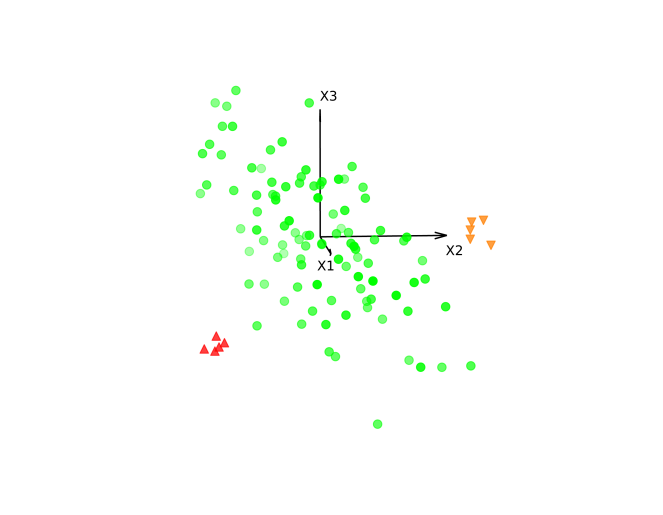
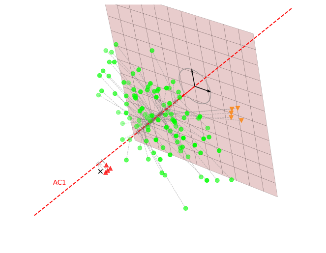
$2^{nd}$ AC (projection view)	Projection in ACA subspace with 2 ACs

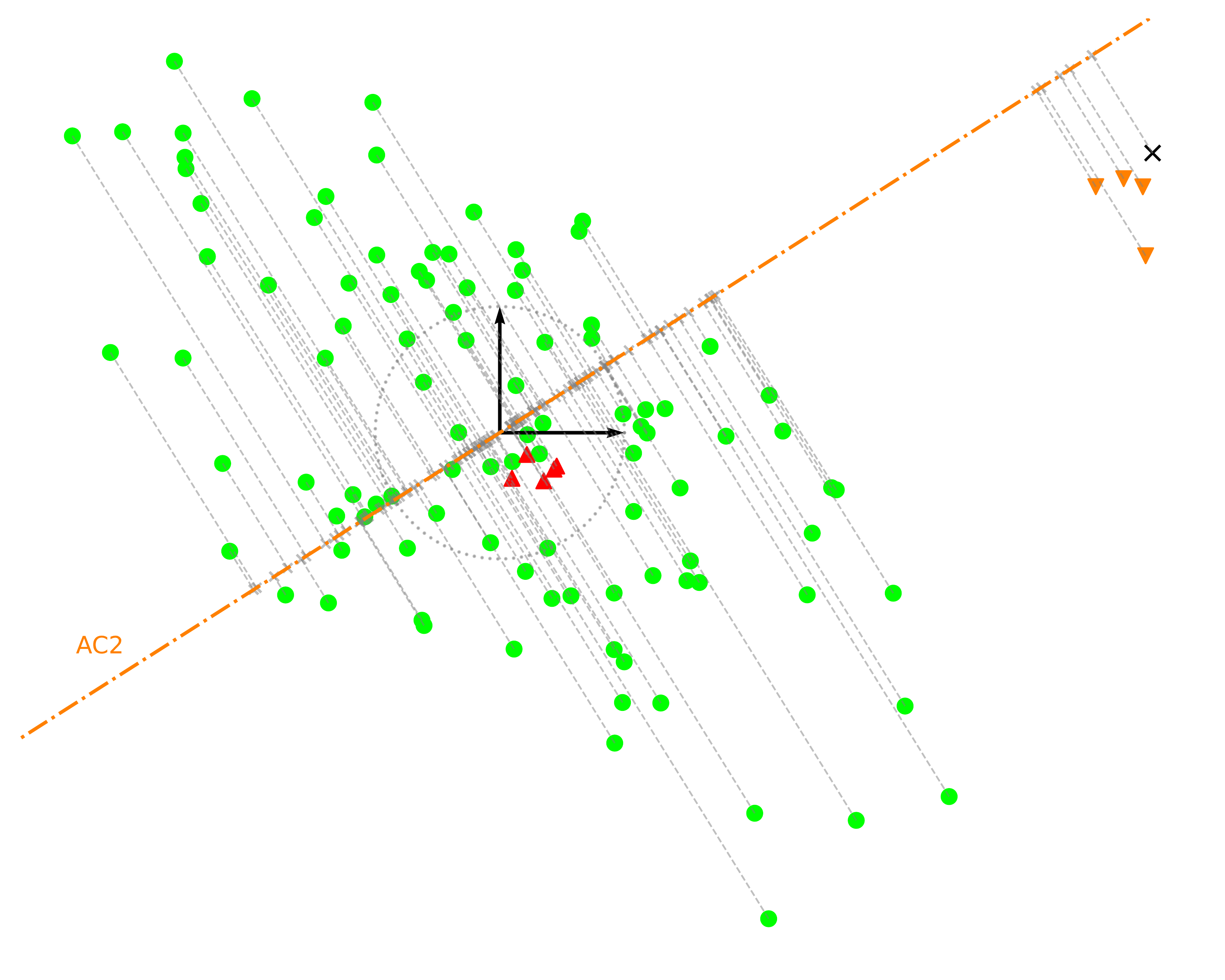
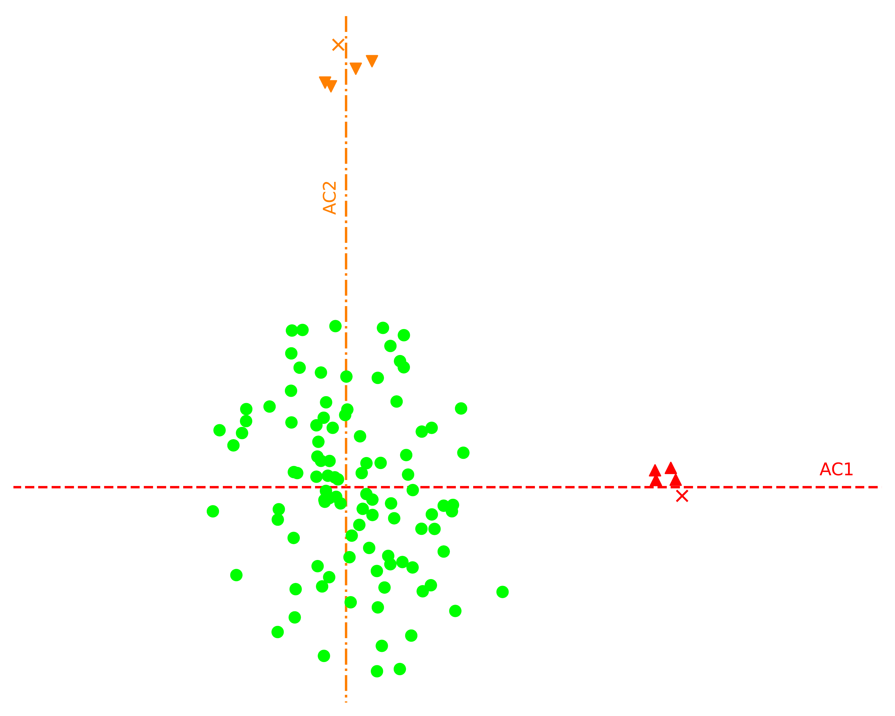
Figure 1: An example of the ACA procedure on a data set containing $n=100$ points in $\mathbb{R}^{3}$ with $10$ anomalies in two groups of $5$.

We start with an intuitive explanation of the ACA method. To facilitate the exposition, let us consider as an example a data set ${\boldsymbol{X}}$ containing $n=100$ points in $\mathbb{R}^{3}$ with $10$ anomalies, in two groups of $5$ anomalies each (red triangles and orange reverse triangles); see Figure 1, top left. It is important to mention, that for data in higher dimensions no visualization is possible. On the first step, a point $\in{\boldsymbol{X}}$ is searched with minimal depth (among the $n$ points), and it’s direction being the argument of (1) ${\boldsymbol{u}}_{1}$ is taken as the first anomaly component (AC). This direction shall clearly identify the most significant group of anomalies (red triangles); see Figure 1, top right. On the second step, again a point $\in{\boldsymbol{X}}$ with smallest depth is searched, while the search space (for ${\boldsymbol{u}}$ in (1)) is now limited to the orthogonal complement of ${\boldsymbol{u}}_{1}$ (red plane in Figure 1, top right; see also Figure 1, bottom left for this bivariate linear space). The minimizing direction ${\boldsymbol{u}}_{2}$, which in order identifies the second group of anomalies (orange reverse triangles) is taken as the second component. Figure 1, bottom right, depicts the constructed bivariate space on the basis of ${\boldsymbol{u}}_{1}$ and ${\boldsymbol{u}}_{2}$, which clearly distinguishes the two groups of anomalies. Although we stop here for our example in $\mathbb{R}^{3}$, the process continues, each time searching in the orthogonal complement of all anomaly components found on the earlier steps.

In the following subsection, we shall formally state the algorithm for ACA in pseudo-code, accompanied with a brief step-wise explanation.

2.3 The algorithm

We start by introducing the following depth computation problem (valid for an arbitrary univariate depth notion $D^{1}$), which is very similar to (1):

$$D_{{\boldsymbol{B}}}({\boldsymbol{z}}|{\boldsymbol{X}})=\min_{{\boldsymbol{u}}\in\mathbb{S}^{{\boldsymbol{B}}}}D^{1}({\boldsymbol{z}}^{\top}{\boldsymbol{u}}|{\boldsymbol{X}}{\boldsymbol{u}})$$ (2)

where $\mathbb{S}^{{\boldsymbol{B}}}$ stands for the unit hyper-sphere in the space spanned by columns of the basis matrix ${\boldsymbol{B}}$. Note, that though real dimension of ${\boldsymbol{u}}$ here is limited by the number of columns in ${\boldsymbol{B}}$, it is a vector (of length $1$) in the original space $\mathbb{R}^{d}$. To be used in what follows, denote projDepth an algorithmic routine which computes (2) and returns both the depth values and its minimizing direction, taking as parameters:

• point ${\boldsymbol{z}}\in\mathbb{R}^{d}$ for which the depth is computed;

• the data set ${\boldsymbol{X}}\subset\mathbb{R}^{d}$;

• the search-basis matrix ${\boldsymbol{B}}$;

• the chosen notion of data depth;

• the number of $k$ directions used to approximate the depth value (see the next Section 2.4 to get insights about the choice of $k$);

• further parameters necessary for the optimization procedure (more details are contained in Dyckerhoff et al., 2021).

A number of useful algorithms for projDepth can be found in Dyckerhoff et al. (2021); we thus simply refer the reader to this article for the computational questions.

Algorithm 1 implements the general ACA method, while Algorithm 2 gathers the steps for finding the $i$th anomaly component.

Algorithm 1 (Anomaly component analysis).

1. Input: ${\boldsymbol{X}}={\boldsymbol{x}}_{1},\cdots,{\boldsymbol{x}}_{n}\in\mathbb{R}^{d}$, $p$, depth, $k$, pars.

2. Step 1: Initialization:

   1. Set $\boldsymbol{A}=[\,]$, $\boldsymbol{B}=\boldsymbol{I}_{d}$.

3. Step 2: Find $p$ anomaly components:

   1. For $i=1,...,p$ do:

      1. $\mathbb{S}^{d}\ni{\boldsymbol{u}}_{i}=$ anomCmp$({\boldsymbol{X}},\,\boldsymbol{B},\,\texttt{depth},\,k,\,\texttt{pars})$.

      2. $\boldsymbol{A}=[\boldsymbol{A},{\boldsymbol{u}}_{i}]$.

      3. $\boldsymbol{B}=\boldsymbol{A}^{\bot}$.

4. Output: $\boldsymbol{A}$.

Algorithm 1 starts with the empty set of anomaly components and the full-space basis $[\boldsymbol{\mathrm{e}}_{1},...,\boldsymbol{\mathrm{e}}_{n}]$ encoded by matrix ${\boldsymbol{B}}={\boldsymbol{I}}_{d}$, with ${\boldsymbol{I}}_{d}$ being the $d\times d$ identity matrix. On each step of Algorithm 1, $i$th anomaly component is (found and) added to the set of components (matrix ${\boldsymbol{A}}$) until the pre-specified number of anomaly components $p$ has been reached. Further, on each step, the size of the basis matrix ${\boldsymbol{B}}$ is reduced by one column so that the basis remains orthogonal to all the found (until $i$th step) components (saved in matrix ${\boldsymbol{A}}$). The search of the $i$th anomaly component is performed by Algorithm 2:

Algorithm 2 (anomCmp).

1. Input: ${\boldsymbol{X}}={\boldsymbol{x}}_{1},\cdots,{\boldsymbol{x}}_{n}\in\mathbb{R}^{d}$, $\boldsymbol{B}$, depth, $k$, pars.

2. Step 1: Initialization:

   1. Set ${\boldsymbol{u}}^{*}=\boldsymbol{0}_{d}$, $D^{*}=1$.

3. Step 2: Minimize over data points:

   1. For $i=1,...,n$ do:

      1. $(D,{\boldsymbol{u}})=$ projDepth$({\boldsymbol{x}}_{i},\,{\boldsymbol{X}},\,\boldsymbol{B},\,\texttt{depth},\,k,\,\texttt{pars})$.

      2. If $D<D^{*}$ then:

         1. $m=\text{med}({\boldsymbol{x}}_{1}^{\top}{\boldsymbol{u}},...,{\boldsymbol{x}}_{n}^{\top}{\boldsymbol{u}})$.

         2. If ${\boldsymbol{x}}_{i}^{\top}{\boldsymbol{u}}<m$ then ${\boldsymbol{u}}=-{\boldsymbol{u}}$.

         3. $D^{*}=D$, ${\boldsymbol{u}}^{*}={\boldsymbol{u}}$.

4. Output: ${\boldsymbol{u}}^{*}$.

Algorithm 2 simply goes through all points $\in{\boldsymbol{X}}$ and selects the one delivering minimal depth:

$$\text{min}D_{{\boldsymbol{B}}}({\boldsymbol{X}})=\min_{{\boldsymbol{x}}\in{\boldsymbol{X}}}\min_{{\boldsymbol{u}}\in\mathbb{S}^{{\boldsymbol{B}}}}D^{1}({\boldsymbol{x}}^{\top}{\boldsymbol{u}}|{\boldsymbol{X}}{\boldsymbol{u}})\,,$$

while the search is performed in the linear subspace of $\mathbb{R}^{d}$ defined by matrix ${\boldsymbol{B}}$, and the minimal-depth-minimizing direction is returned in addition to the depth value. The search is implemented by the means of the algorithmic routine projDepth described above, and the obtained direction is assured to have anomalies on its positive side. In order to do this, the depth notion, the number of directions used for depth approximation, as well as further algorithmic parameters shall be chosen; we discuss these right below in the following subsection.

Algorithm 1 possesses complexity $\mathcal{O}(pkdn^{2})$ which can be decomposed as follows: with number of searched components $p$, number of depth-approximating directions $k$, dimension $d$ obviously entering linearly in the complexity, $n^{2}$ is explained by the fact that, for each component, all $n$ points should be revisited while each time all $n$ points should be projected on each direction (inside the optimisation routine projDepth). While approximation accuracy is clearly dependent on $k$, one can suppose it’s polynomial dependence on $d$. In this article, we employed the spherical modification of the Nelder-Mead algorithm delivering best results as studied by Dyckerhoff et al. (2021). Regarding the accuracy, which (though not exact) can still be sufficient for components’ search: (a) the work by Nagy et al. (2020) sheds the light on algorithmic convergence of the simplest approximation techniques and (b) chosen values of $k$ in practice delivered highly satisfactory results in all experiments conducted for this article. Right below, we discuss further the choice of parameters when performing ACA.

2.4 Choice of parameters

When applying ACA, several parameters need to be set:

• number of anomaly components to search,

• the notion of data depth,

• number of directions used to approximate point’s depth,

• optimization parameters;

we discuss these choices in detail right below.

Number of anomaly components

As in any dimension reduction (or visualization) method, dimension of the obtained space $p\in\{1,...,d\}$ is guided either by prior knowledge about the data (generating process) or by computational resources (needed for further analysis). Though the choice of $p$ is entirely heuristic, it can be guided by a priori information about (expected) anomalies in the data, e.g., possible dimension of anomalies’ subspace or number of their groups.

Depth notion

The chosen notion of statistical depth function can have an important influence on the ACA’s performance. Throughout this article, we stick to the notion of the projection depth, with sparse use of the asymmetric projection depth (see Section 4.2 below), for the reasons mentioned in Section 2.1. For a detailed discussion on the choice of depth notion in the multivariate setting we refer the reader to the recent survey by Mosler and Mozharovskyi (2022). Furthermore, theoretically, any (efficiently optimizable) univariate directional score can be used instead as well; a precaution shall be exercised regarding its eventual statistical properties though.

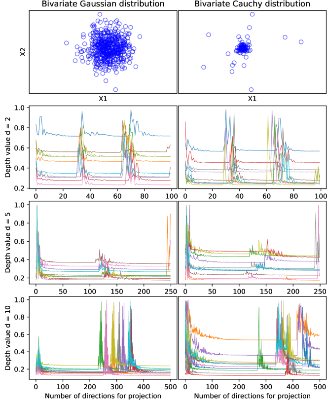
Figure 2: Tuning process for the number of directions $k$, on the example of $10$ points from a sample stemming from (non-correlated) Gaussian (left) and Cauchy (right) distribution, in dimensions $d=2,5,10$.

Number of directions

The number of directions $k\in\mathbb{N}_{+}$ has a profound influence on the precision of depth computation, and thus on the found direction(s) of anomaly component(s). Nagy et al. (2020) prove that, even for the probability distribution, the number of $k$ shall grow exponentially with dimension for uniformly good depth approximation, if these directions are drawn at random. Further, Dyckerhoff et al. (2021) show that this number can be substantially reduced when using (adapted to the task) optimization algorithm, hopefully (and at least heuristically) departing from the exponential dependency on $d$, and indicate that in experiments where dimension is up to $d=20$ the (zero-order) optimization algorithm can converge fast requiring only few hundred directions. In their work, the authors propose a comprehensive comparison of number of algorithms in various settings with the lead taken by the Nelder-Mead algorithm, the sphere-adjusted coordinate descent, and the refined random search.

To decide on the number of directions in the application at hand, we suggest the following simple verification following the very principle of the class of depths satisfying the projection property (1): “the smaller the approximated depth value the better it is”. That being said, even without knowing the true depth value, it is reasonable to choose the method and number of directions delivering the smallest depth value. A simple way to study the optimization behavior is the visual inspection of the development of the (minimal) depth value throughout the optimization iterations, for at least several points from the data set. For a sample from Gaussian and Cauchy distribution (with varying dimension), this is illustrated in Figure 2, where the repeating jumps of the depth value indicate re-starting the optimization routine in hope to avoid local minima.

Optimization parameters

To obtain more insights about the choice of the optimization parameters, including the optimization algorithm itself, the reader is referred to the article by Dyckerhoff et al. (2021). Furthermore, the above described methodology on a subset of ${\boldsymbol{X}}$ can be employed here, as well as in a larger simulation setting resembling the real data at hand.

3 Visual comparison

In this section, visualization capacity of ACA is explored in a comparative simulation study. After a brief discussion on present visualization tools and existing problems (Section 3.1) we present the simulation settings (Section 3.2). Further, Section 3.3 presents the results compared to those obtained with most used (interpretable) dimension reduction methods, while the rest is preserved for the real-data study in Section 5.

3.1 On existing dimension-reduction tools

With the task of Section 3 being examination of ACA’s performance in dimension-reduction compared to existing methods, we shall start with selecting from the state of the art. For interpretability reasons, methods with linear—in input variables—components will be preferred.

With PCA being the natural candidate due to it’s wide spread, including robPCA as well is necessary in presence of anomalies, for fair comparison. Here, robPCA is employed in the same manner as traditional PCA where the mean and covariance matrix are estimated robustly, using the minimum covariance determinant (MCD, see Rousseeuw and Leroy, 1987; Lopuhaa and Rousseeuw, 1991) with the standard value for parameter $\alpha=(n+d+1)/2n$ (portion or anomalies in all our experiments never exceeds this parameter); see also Rousseeuw and Driessen (1999) for the fast randomized algorithm. To allow for ’non-Gaussian’ methodology, we further include ICA. Finally, we include auto-encoder, being a widely used neural-network-based tool able to learn highly non-linear components, it provides a visualization in form of (latent) variables of the ’bottle-neck’ layer. (The auto-encoder used has 10-5-2-5-10 layers and was trained using the stochastic gradient descent algorithm with $\mathbb{L}_{2}$ loss during 100 epoch with mini-batch size 10 and learning rate 0.005.)

Further methods like kPCA, $t$-SNE, MDS, LLE, or LE, though based on components non-linear in input variables, constitute powerful dimension-reduction machinery and can also provide insightful visualization. Due to this non-linearity property, but also for conciseness, we skip them in this simulation comparison, while include later in Section 5 for analysis of real data.

Though mentioned above for completeness, we exclude NMF due to the positivity of components (which is not justified for general types of data, but only in specific applications, e.g., audio signals, images, text etc).

Setting 1: MVN(A09)	Setting 2: MVN(hCN)
Setting 3: ELL($t(5)$)	Setting 4: EXP

Figure 3: Example (in $\mathbb{R}^{2}$) of a data sample for four contaminated settings: MVN(A09) (top, left), MVN(hCN) (top, right), EXP (bottom, left), ELL($t(5)$) (bottom, right).

3.2 Explored simulation settings

Below, we describe five distributional settings (for normal data) used in the current visualization comparison, but also later throughout the article. Here, all of them follow the (famous and most adapted in the literature) Huber’s contamination model Huber (1964, 1965):

$$Y\stackrel{{\scriptstyle\mathcal{D}}}{{=}}(1-\epsilon)X+\epsilon\widetilde{X}\,,$$ (3)

where the random vector $X$ (e.g., here, in $\mathbb{R}^{d}$) represents normal data while $\widetilde{X}$ stands for outliers (and $\stackrel{{\scriptstyle\mathcal{D}}}{{=}}$ denotes equality in distribution). More precisely, in a sample of size $n$, the $\lfloor n\cdot(1-\epsilon)\rfloor$ points of normal data are generated according to one of the following scenarios:

• Setting 1 – MVN(A09): Normal data are generated as i.i.d. copies of the multivariate-normally distributed random vector:

  $$X\sim\mathcal{N}\bigl{(}\boldsymbol{0}_{d},\boldsymbol{\Sigma}_{A09(d)}\bigr{)}\,,$$

  where $\boldsymbol{\Sigma}_{A09(d)}$ consisting of $\{\sigma_{i,j}\}_{i,j=1}^{d}$ is the Toeplitz matrix with $\sigma_{i,j}=0.9^{|i-j|}$, i.e., to ensure various values of correlation between different variables; see (Rousseeuw and Bossche, 2018) for precisely this form.

• Setting 2 – MVN(hCN): This setting copies MVN(A09) where the covariance matrix is a matrix with high condition number ($=100$, following Agostinelli et al., 2015, see Section 4 for the exact matrix-generating procedure).

• Setting 3 – ELL($t(5)$): Multivariate elliptical Student-$t(5)$ distribution:

  $$X\stackrel{{\scriptstyle\mathcal{D}}}{{=}}\boldsymbol{\mu}+\boldsymbol{\Lambda}UR\,,$$

  where $U\sim\mathcal{U}(\mathbb{S}^{d-1})$ is uniformly distributed on the unit hypersphere, $R\sim St(5)$ is a Student-$t(5)$-distributed random variable, $\boldsymbol{\Lambda}\boldsymbol{\Lambda}^{\top}=\boldsymbol{\Sigma}$, and $\mathbb{R}^{d}\ni\boldsymbol{\mu}(=\boldsymbol{0}_{d})$ and $\boldsymbol{\Sigma}=\boldsymbol{\Sigma}_{A09(d)}$ are the distribution’s center and scatter, respectively. ELL($t(5)$) has heavier tails than MVN(A09).

• Setting 4 – EXP: Random vector of normal data is here:

  $$X=(X_{1},...,X_{d})^{\top}\quad\text{with mutually independent}\quad X_{i}\sim\mathcal{E}(\lambda_{i})\,,i=1,...,d\,,$$

  where $X_{i}$s are $d$ exponentially distributed random variables with parameters $\lambda_{i}=\frac{1}{\beta_{i}}\text{ and }\beta_{i}\sim\mathcal{U}([0.1,1])$. EXP is asymmetric and possesses high degrees of skewness w.r.t. different variables.

• Setting 5 – MV-Sk: Bivariate normal distribution skewed along the first variable according to Azzalini and Capitanio (1999):

  $$X=(X_{1},X_{2})^{\top}\quad\text{with}\quad X_{1}\sim\mathcal{N}_{Sk}\bigl{(}0,1,\alpha\bigr{)}\quad\text{and}\quad X_{2}\sim\mathcal{N}\bigl{(}0,1/4\bigr{)}\,,$$

  where $\alpha=10$ is the skewness parameter.

3.3 Two-dimensional plots

In this section we shall focus on first four settings from Section 3.2 in order to compare the components-based visualization, while letting MV-Sk for Section 4.2. Fixing the portion of anomalies to $\epsilon=0.05$, in each case we generate the $n-\lfloor n\cdot(1-\epsilon)\rfloor$ contaminating data from $\widetilde{X}\sim\mathcal{N}(\boldsymbol{0}_{d},\boldsymbol{I}_{d}/20)$ placed in direction of the last principal component of PCA of normal data centered at the distance of $1.25\,\times$ the largest Mahalanobis distance among normal data points. We thus obtain $\boldsymbol{Y}=\{{\boldsymbol{y}}_{1},...,{\boldsymbol{y}}_{n}\}$ by fixing $n=1000$ and $d=10$. It is important to note that concentrating the contaminating cluster of $\widetilde{X}$ on the last principal component does not influence the generality of conclusions but simplifies the presentation; we shall comment this more in detail right below when analysing the PCA output. For illustrative purposes, we plot a data sample from each of the four contaminated settings in $\mathbb{R}^{2}$ in Figure 3.

PCA for MVN(A09)	PCA for MVN(hCN)
PCA for ELL($t(5)$)	PCA for EXP

Figure 4: Projection of data set ${\boldsymbol{Y}}$ on first two components obtained by PCA.

PCA

Figure 4 plots ${\boldsymbol{Y}}$’s projection on first two components obtained by application of PCA. While it is not surprising that—with first two components—PCA is not able to ‘notice’ anomalies located in direction of the $10$th component in $\mathbb{R}^{10}$, this example is illustrative and by no means restrictive, for the three following reasons:

• It is a reasonable frequent practice, to pre-process data using dimension-reduction techniques (like PCA) and then apply statistical (e.g., anomaly detection) method in the space of several first and several last components. From this point of view, if the component with anomalies (independent of it’s number) is not taken over into the reduced space, anomalies remain unnoticed for most visualization and analysis tools.

• If correlation (or a higher-order stochastic dependency) is present in the data, (small number of) anomalies cannot be noticed in any (e.g., $2=$) $k$-dimensional projection if they are placed on, e.g., the average of $k+1$ ($=3$) correlated components, being shadowed by $k$-dimensional marginals.

• For a practitioner interested in identifying (and explaining) anomalies, it is in any case advantageous if anomalies are explicitly highlighted by first component(s).

robPCA for MVN(A09)	robPCA for MVN(hCN)
robPCA for ELL($t(5)$)	robPCA for EXP

Figure 5: Projection of data set ${\boldsymbol{Y}}$ on first two components obtained by robPCA.

robPCA

Projection of ${\boldsymbol{Y}}$ on two first components obtained by robPCA, for the four mentioned above contaminated settings, is depicted in Figure 5. Using robust MCD estimates for the mean and covariance matrix, the group of anomalies is being ignored, and principal components well approximate the variance-maximizing directions (e.g., for MVN and ELL they are close to the axes of the ellipsoids defined by the population (=true) covariance matrix). With anomalies not necessarily lying on the first (or in general no) such axes, they are not readily identifiable/explainable from the visualization.

ICA for MVN(A09)	ICA for MVN(hCN)
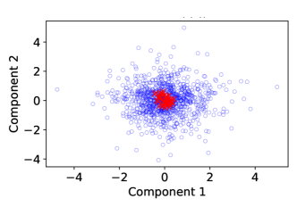
ICA for ELL($t(5)$)	ICA for EXP

Figure 6: Projection of data set ${\boldsymbol{Y}}$ on first two components obtained by ICA.

ICA

Further, though anomalies-highlighting directions are (obviously) linear in variables, as expected, without an anomaly-specific criterion employed when searching components, the picture does not change for ICA; see Figure 6.

Auto-encoder

To visualize the data representation using auto-encoder, we exploit its bottle-neck where information about noisy observations is expected to be filtered out. Thus, we use output of the two neurons of the third layer as latent variables, plotted for ${\boldsymbol{Y}}$ in Figure 7. The intrinsic smoothness assumption on the approximable by neural network function makes them generally more vulnerable to increasing portions of anomalies (in the training sample) than traditional methods of robust statistics. Generally speaking, even when auto-encoder properly distinguishes anomalies by their reconstruction loss (which is not the case here), finding a low-dimensional anomaly-insightful representation can still be challenging, especially in realistic situations where the number of bottle-neck neurons is substantially larger than $2$.

Auto-encoder for MVN(A09)	Auto-encoder for MVN(hCN)
Auto-encoder for ELL($t(5)$)	Auto-encoder for EXP

Figure 7: Projection of data set ${\boldsymbol{Y}}$ on two latent components of the bottle-neck of auto-encoder.

ACA

Non surprisingly, being designed for highlighting anomalies, and directly targeting them when searching for components, ACA copes with this artificial task, with contaminating ${\boldsymbol{Y}}$ anomalies being located (and centered) on the first component. With ${\boldsymbol{Y}}$ being rather a simple illustrative example, in what follows we switch to further aspects of ACA as well as to more challenging settings.

4 Explainability

The intrinsic linearity of the ACA method positions it as a powerful tool for explainability—a highy demanded property in the domain of unsupervised anomaly detection. Here, different to supervised setting, no feedback can provide a criterion to decide about importance of a variable, with the goal being to explain how a variable contributes to the method’s decision about abnormality of an observation. The framework of ACA suggests possibilities to identify most deviating variable(s) for each anomaly.

With each ACA’s anomaly component (further AC) being a linear combination of the (input) variables, their contributions (perhaps properly re-scaled) highlight variables’ abnormalities. Before exploiting this information (see Section 4.2), let us first pay attention to the ACs themselves.

ACA for MVN(A09)	ACA for MVN(hCN)
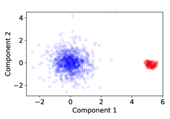
ACA for ELL($t(5)$)	ACA for EXP

Figure 8: Projection of data set ${\boldsymbol{Y}}$ on first two components obtained by ACA.

4.1 Direction that highlights abnormality

According to the principle of projected outlyingness (Stahel, 1981; Donoho, 1982), an AC (i.e., the corresponding direction) should be chosen in a way so that—in projection on it—abnormal observation(s) (cluster) is best separated from normal data. The goal of this subsection is to benchmark usefulness of the generated ACs in the elliptical setting, where a reasonable guess is easier to find theoretically. More precisely, the found direction (let us name it ${\boldsymbol{u}}^{*}_{1}$) should be such that it best separates the anomaly (or anomalies’ cluster) from normal data. In the elliptical setting, a good candidate is the direction orthogonal to the—tangent to any ellipsoid—hyperplane that contains the abnormal point of interest. For comparison, let us fix this point to the earlier defined $\boldsymbol{\tilde{\mu}}\in\mathbb{R}^{d}$ (see Section 3.3). Then, a good candidate for the searched direction is ${\boldsymbol{u}}^{*}_{1}=\frac{\boldsymbol{\Sigma}^{-1}\boldsymbol{\tilde{\mu}}}{\|\boldsymbol{\Sigma}^{-1}\boldsymbol{\tilde{\mu}}\|}$, with $\boldsymbol{\Sigma}$ standing for the covariance matrix of the elliptical distribution. From this point of view, effectiveness of a dimension-reduction method, which—when applied to data set ${\boldsymbol{Y}}\subset\mathbb{R}^{d}$—returns up to $m\leq d$ ordered (with decreasing importance) component vectors ${\boldsymbol{u}}_{1},...,{\boldsymbol{u}}_{m}$, can be naturally measured by two indicators:

• index of component that is most aligned with ${\boldsymbol{u}}^{*}_{1}$ (for most fair comparison),

  $$\hat{i}=\operatornamewithlimits{argmin}_{i\in\{1,...,m\}}\,\text{arc\,cos}({\boldsymbol{u}}_{i}^{\top}{\boldsymbol{u}}^{*}_{1})\,,\quad\text{and}$$

• the corresponding angle:

  $$\hat{\alpha}=\text{arc\,cos}({\boldsymbol{u}}_{\hat{i}}^{\top}{\boldsymbol{u}}^{*}_{1})\,.$$

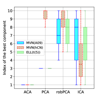
Figure 9: For the component having smallest angle with ${\boldsymbol{u}}_{1}^{*}$ obtained with ACA, PCA, robPCA, and ICA, boxplots of its index ($\hat{i}$, left) and angle to ${\boldsymbol{u}}_{1}^{*}$ ($\hat{\alpha}$, right); for MVN(A09), MVH(hCN) and ELL($t(5)$), over $50$ random draws of ${\boldsymbol{Y}}$.

For the three elliptical distributions from Section 3.2 (MVN(A09), MVN(hCN), and ELL($t(5)$)) contaminated as described in Section 3.3, we plot in Figure 9 $\hat{i}$ and $\hat{\alpha}$ for ACA, PCA, robPCA, and ICA. Note, that since the angle is measured as a positive value, the error in itself is inevitable, in particular for the empirical case. While it is expected that components with higher index numbers can be better aligned with the anomalies-explaining direction for other methods, their angles are still much higher that those of ACA (which always identifies anomalies with the first component). Furthermore, variables contributing more to this direction can be seen as responsible for the abnormality.

4.2 Focus on variable’s contribution

Following the principle of ACA, in this section, we shall explore the general capacity of (asymmetric) projection depth to highlight variables responsible for observations’ abnormality, in two comparative simulation studies.

$\gamma=0.8$	$\gamma=0.9$
$\gamma=1$	$\gamma=1.5$

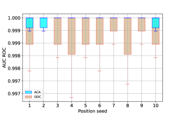
Figure 10: AUC of cells’ anomaly scores attributed by DDC and ACA’s directions for 1000 bivariate observations drawn from MV-Sk setting; 50 simulations are performed for each of $10$ position seed values.

Comparison with DDC

Rousseeuw and Bossche (2018) proposed a method for detecting (and imputing) deviating data cells (DDC) in the data set, which can be also seen as explaining anomaly-detection tool. (Under a cell-wise anomaly one understands a normal observation whose one or more coordinates are contaminated with other variables remaining intact.) In what follows, we shall compare (asymmetric) projection depth with DDC in detecting such deviating cells. With DDC exploiting correlation, we use the following challenging anomaly-detection setting: we generate ${\boldsymbol{Y}}$ according to MV-Sk (see Section 3.2) contaminated with $10\%$ of anomalies from Section 3.3 restricting $\boldsymbol{\tilde{\mu}}$ to the set $\gamma M_{max}{\boldsymbol{u}}\,:\,\{{\boldsymbol{u}}^{(1)}>0,\,\|{\boldsymbol{u}}^{(2)}\|>{\boldsymbol{u}}^{(1)},\,{\boldsymbol{u}}\in\mathbb{S}^{d-1}\}$ (with ${\boldsymbol{u}}^{(i)}$ denoting $i$th coordinate of ${\boldsymbol{u}}$ and $M_{max}$ standing for the maximal Mahalanobis distance among normal data); we set $\gamma=0.8,0.9,1,1.5$, $n=1000$ and $d=2$ (see the Supplementary Materials, Section 3 for a visualization of the data generating process). Thus, ${\boldsymbol{Y}}$ is not only asymmetric, but as well all anomalies are trivially explained by the second variable.

For $i$th variable of ${\boldsymbol{y}}$, the depth-based anomaly score is constructed as:

$$s^{(i)}({\boldsymbol{y}}|{\boldsymbol{Y}})=\|{\boldsymbol{u}}_{pd}^{(i)}({\boldsymbol{y}}|{\boldsymbol{Y}})\|\,\cdot\,\bigl{(}1/D^{apd}({\boldsymbol{y}}|{\boldsymbol{Y}})-1\bigr{)}\,,$$

where ${\boldsymbol{u}}_{pd}({\boldsymbol{y}}|{\boldsymbol{Y}})\in\operatornamewithlimits{argmin}_{{\boldsymbol{u}}\in\mathbb{S}^{d-1}}D^{pd}({\boldsymbol{y}}|{\boldsymbol{Y}})$. For DDC, to each observation’s variable we attribute the cell’s standardized residuals as anomaly score (see Rousseeuw and Bossche, 2018, for more details); see also the Supplementary Materials (Section 3) for an example of cell-wise scores’ visualization. Using these scores to order observations in ${\boldsymbol{Y}}$, we compare them to true anomalies by the area under the receiver operating characteristic (AUC); these are indicated in Figure 10. We observe that, under asymmetric deviation from elliptical contours (perfectly described by correlation) DDC is outperformed by the non-parametric depth-based approach in this setting (see also Section 3.2 of the Supplementary Materials for a one-sample visualization of the obtained score). For a broader setting, i.e., when letting more freedom for $\boldsymbol{\tilde{\mu}}$, DDC and depth perform comparably (see Section 3.1 of the Supplementary Materials).

Comparison with DIFFI

Carletti et al. (2023) introduced depth-based isolation forest feature importance (DIFFI) that allows to evaluate contribution of each variable to the abnormality of an observation, and thus constitutes a natural candidate for comparison. We generate data from MVN(A09) and contaminate them with $10\%$ of anomalies generated from from $\mathcal{N}(\boldsymbol{\tilde{\mu}},\boldsymbol{I}_{d}/1000)$ with

$$\boldsymbol{\tilde{\mu}}=\bigl{(}(2\cdot d)^{2},(2\cdot(d-1))^{2},...,(2\cdot 1)^{2}\bigr{)}^{\top}\,,$$ (4)

i.e., variables’ importance decreases in their literal order. For ACA, the variable importance is derived from the variable’s contribution (in absolute value) to the first AC. The resulting order correlation (with the correct order induced by (4)) is indicated in Figure 11 (left), for varying space dimension $d$. One observes that ACA preserves good correlation level when $d$ increases. Not to disadvantage DIFFI, we also attempt the spherical (standard) normal distribution instead of MVN(A09); see Figure 11 (right).

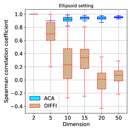
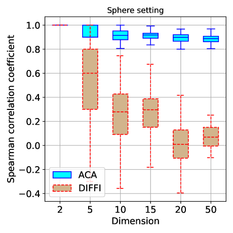
Figure 11: Spearman correlation coefficient (over $50$ repetitions) of variables’ importance ranking (with the population order) for ACA and DIFFI for elliptical (MVN(A09), left) and spherical (right) standard normal distribution.

5 Application to real data sets

Name	$\boldsymbol{n}$	$\boldsymbol{d}$	# Anomalies	% Anomalies	Category
Musk	3062	166	97	3.17	Chemistry
Satellite image (2)	5803	36	71	1.22	Astronautics
Thyroid	3772	6	93	2.47	Healthcare

Table 1: Information on real-world data sets.

Next, we explore the performance of both visualization and explainability provided by ACA in a comparative real-data study. For this, we address $7$ real-world data sets downloaded from Rayana (2016), and present $3$ of them right below (see Table 1 for brief information), with further $4$ (for space reasons) being shifted to the Supplementary Materials, see Section 4). For each of them, we contrast ACA with $9$ dimension-reduction methods PCA, robPCA, kPCA, ICA, AE, $t$-SNE, MDS, LLE, and LE (see Section 1.1 for a brief overview with references), by visualizing projection on first two components.

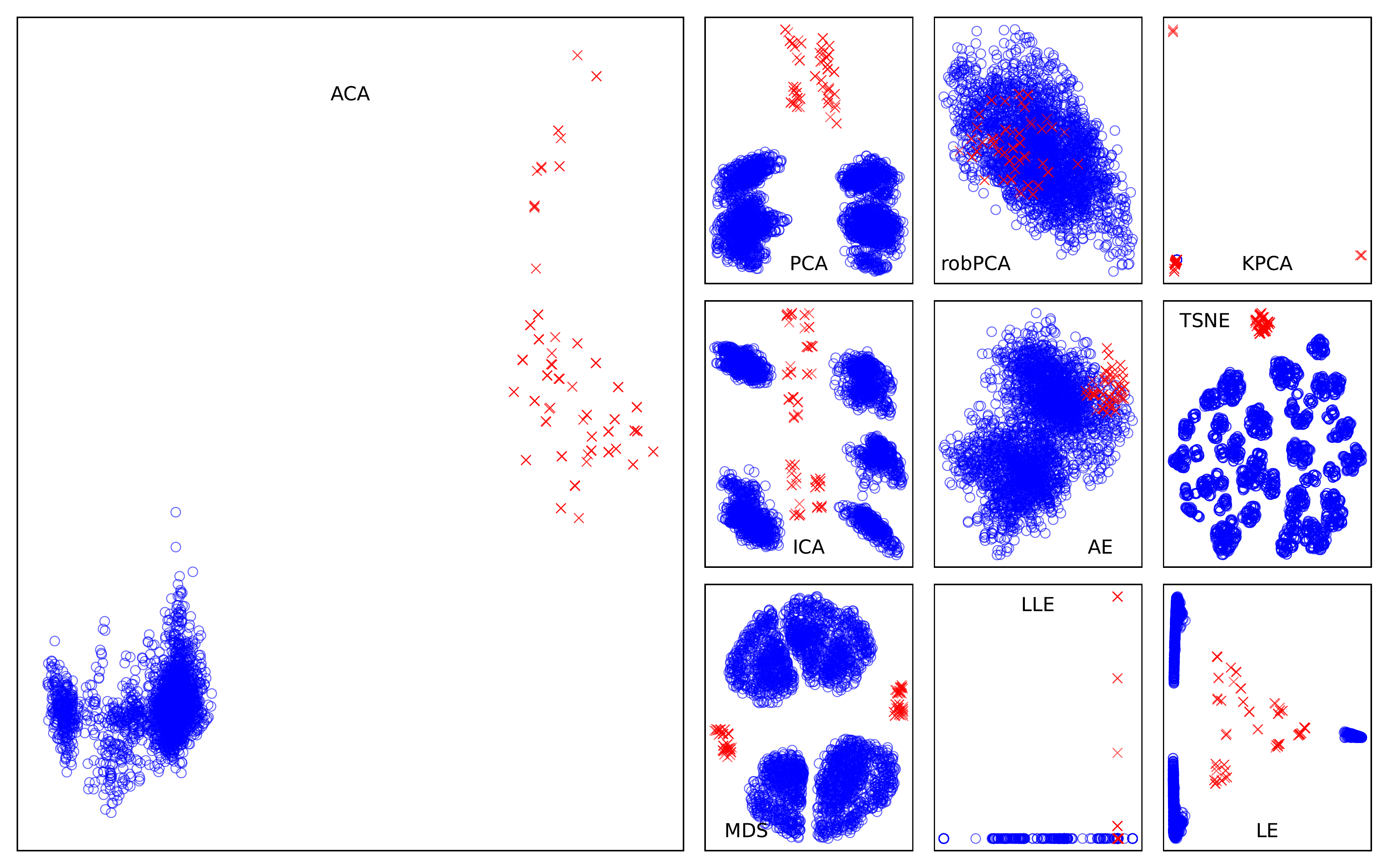
Figure 12: Visualization of projection on two first components obtained by different methods for Musk data set.

	Musk data set
	PCA		robPCA		ICA		ACA
	PC1	PC2	robPC1	robPC2	IC1	IC2	AC1	AC2
Var1	114 (1%)	102 (2%)	165 (13%)	3 (3%)	30 (2%)	62 (6%)	44 (3%)	5 (6%)
Var2	113 (1%)	155 (2%)	163 (12%)	68 (2%)	128 (2%)	32 (6%)	105 (3%)	155 (2%)
Var3	99 (1%)	96 (2%)	164 (4%)	41 (2%)	64 (2%)	125 (5%)	14 (2%)	46 (2%)

Table 2: Contributions of three most important (for each component) variables for PCA, robPCA, ICA, and ACA for Musk data set.

Musk data set

Musk data set contains molecules described by $166$ features extracted from low-energy conformation, with a part being marked as musk ($=$anomalies) by experts; variables are hence further indexed by integers here. Visualization of projection on first two components (Figure 12) reveals that ACA precisely distinguishes anomalies by their projection on AC1 (with projection on AC2 being shifted as well). While some other methods (PCA, ICA, $t$-SNE, MDS, LE) also isolate them, detecting those further (say, in an automatic way) is less obvious. It is further interesting to consider the components’ constitution (for methods with linear variables’ combinations); see Table 2, with percentages being low due to high number of variables. Thus, only ACA identifies importance of variables ($=$conformations’ features) ‘44’ and ‘105’ for abnormality, while solely variable ‘155’ (in AC2) also appears in PCA.

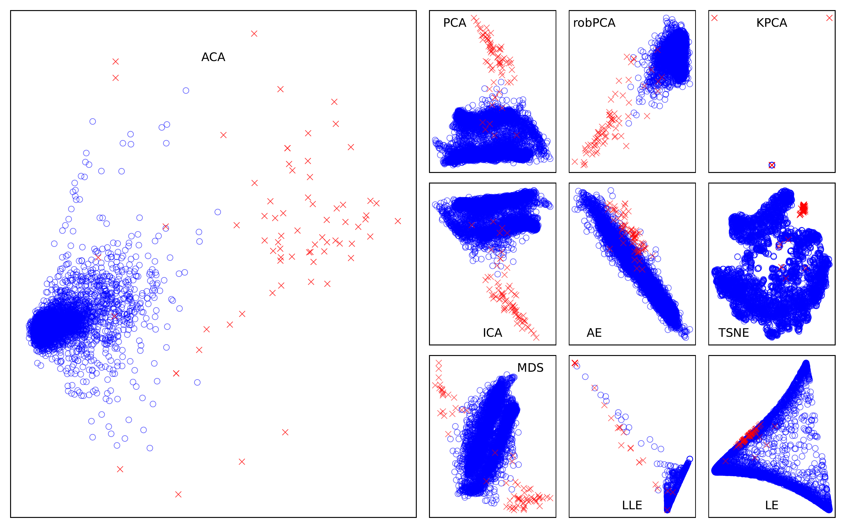
Figure 13: Visualization of projection on two first components obtained by different methods for Satellite image (2) data set.

	Satellite image (2) data set
	PCA		robPCA		ICA		ACA
	PC1	PC2	robPC1	robPC2	IC1	IC2	AC1	AC2
Var1	19 (3%)	17 (5%)	24 (7%)	25 (6%)	19 (4%)	13 (4%)	18 (8%)	12 (9%)
Var2	15 (3%)	13 (5%)	35 (7%)	13 (6%)	23 (4%)	17 (4%)	2 (8%)	10 (8%)
Var3	18 (3%)	29 (5%)	15 (6%)	18 (6%)	31 (4%)	5 (4%)	26 (6%)	8 (7%)

Table 3: Contributions of three most important (for each component) variables for PCA, robPCA, ICA, and ACA for Satellite image (2) data set.

Satellite image (2) data set

This data set contains multi-spectral values of pixels in $3\times 3$ neighborhoods in a satelite image, with one of the classes (Class 2) being downsampled to $71$ anomalies. (Variables are also numbered by integers here.) As one can observe from the bi-component visualization, ACA distances anomalies already on AC1, while only PCA, robPCA and ICA preserve them on a second (linear) component; see Figure 14. Out of variables ‘18’, ‘2’, and ‘26’ spotted by AC1, only the first one finds itself 3rd on PC1; see Table 3.

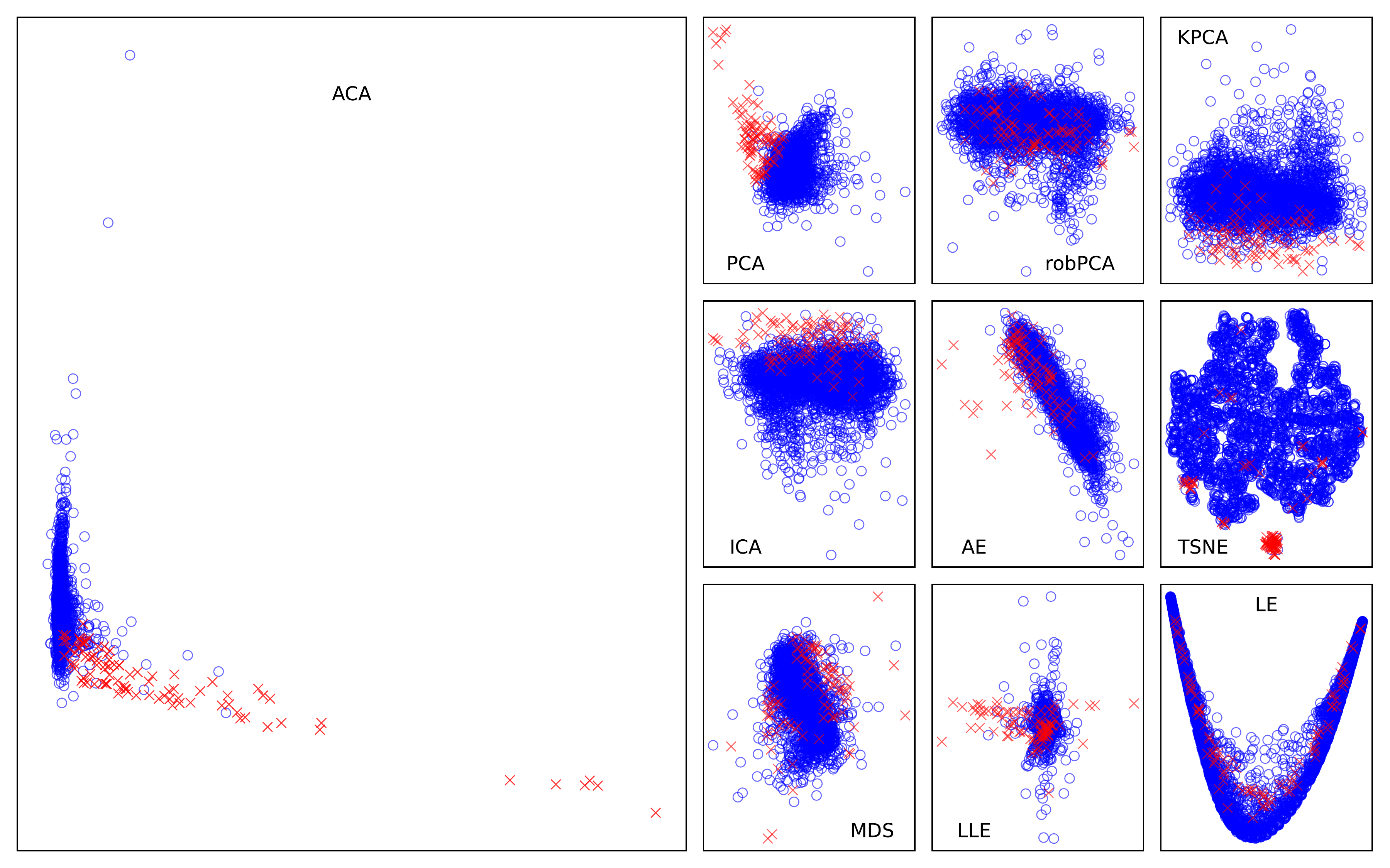
Figure 14: Visualization of projection on two first components obtained by different methods for Thyroid data set.

	Thyroid data set
	PCA		robPCA		ICA		ACA
	PC1	PC2	robPC1	robPC2	IC1	IC2	AC1	AC2
Var1	4 (28%)	5 (28%)	1 (90%)	5 (91%)	1 (73%)	4 (33%)	2 (75%)	6 (64%)
Var2	6 (22%)	1 (21%)	3 (4%)	6 (8%)	4 (11%)	5 (26%)	6 (12%)	4 (18%)
Var3	3 (22%)	6 (20%)	4 (4%)	4 (1%)	6 (6%)	3 (22%)	4 (8%)	2 (12%)

Table 4: Contributions of three most important (for each component) variables for PCA, robPCA, ICA, and ACA for Satellite image (2) data set.

Thyroid data set

For the Thyroid data set, we used $6$ continuous variables where the hyperfunction class is taken as abnormal. Here, visually (Figure 14), ACA outperforms the rest of the methods in addition to being the only one that highlights variable ‘2’ (Triiodothyronine (T3) test) as the main one to explain anomalies, further giving much importance to variable ‘6’ (TBG blood test); see also Table 4.

6 Conclusion

While today a universe of dimension-reduction methods is at practitioner’s disposal, covering different conceptual approaches and application domains, these methods (be it a simple classical method like PCA (or its robust version) or more advanced techniques, e.g., $t$-SNE) are primarily aimed at finding a relevant representation space for the whole empirical data distribution and not at identifying anomalies. Even if in some case general dimension-reduction methods allow to detect or visualize some of them, this happens rather by chance as witnessed in the simulations of Section 3 and real-data examples of Section 5. The only way to get around anomalies is to search for them directly. ACA constitutes an attempt to fill this gap, aiming at representation of anomalies in a linear subspace of the original space $\mathbb{R}^{d}$.

ACA is easy to implement and mainly leverages standard existing (depth-computation and some further) tools with restriction of the direction ${\boldsymbol{u}}$’s search space to a lower-dimensional basis ${\boldsymbol{B}}$ being the only exception. As we discuss in Section 2.3, ACA can be implemented with sufficient precision and polynomial complexity in both data set size $n$ and space dimension $d$. Numerous examples of this article prove reasonable approximation of such implementation in practice. Furthermore, involvement of ${\boldsymbol{B}}$ can be avoided by simply projecting the data on the orthogonal complement of the most recent found component; this would yield a somewhat different procedure though.

Positioning in the anomaly detection framework, ACA constructs an orthonormal basis of a pre-defined dimension, which—hopefully—provides insights on the location of anomalies from the training data set. When projecting new (out-of-sample) data in the same basis, different situations can arise, depending on the contamination model. In case of Huber model (3), the representation should be normally sufficient for gaining insights about anomalies, which should not be necessarily the case for others, in particular adversarial contamination (see, e.g., Diakonikolas et al., 2016; Bateni and Dalalyan, 2020) that can appear in any part of $\mathbb{R}^{d}$ and be shaded by the normal data in all $2$- and $3$-dimensional projections. A possible strategy to act is then to compute the depth/outlyingness of suspected (or all) observations, and if these values indicate potential abnormality, (re-)run ACA on a data set including these observations.

ACA is not restricted to (asymmetric) projection depth only, and can be readily employed with other depth notions that satisfy (1), as well as those minimizable over projections, as it is the case for, e.g., weighted halfspace depth of Kotík and Hlubinka (2017). Moreover, any further procedure that provides an anomaly score based on a univariate data’s projection can be adapted to ACA framework as well. Furthermore, ACA can be extended to data sets in spaces where linear combination of variables is expected to provide a reasonable explanation of anomalies and the corresponding search procedure can be constructed.

With the most relevant information and illustrations incorporated in the body of the article, the Supplementary Materials to this article contain:

• Section 1: additional information on simulation settings from Section 3.2;

• Section 2: full $10$ coordinates constituting anomaly components for visualizations from Section 3.3;

• Section 3: further details on comparison with DDC from Section 4.2;

• Section 4: visualization and components’ data on the $4$ remaining real data sets.

These supplementary materials contain additional information on the study of the performance of the anomaly component analysis (ACA) procedure. First, they contain information about the settings used in the visualisation comparison (Section 1), and detailed results (mentioning every component) concerning all the methods involved in experiments (Section 2). Further, another experiment is presented, similar to the one in the body of the article, with DDC where its performance is closer to that of ACA, as well as information on generation process where the performances differ (Section 3). Finally, other real data sets are used to apply ACA for visualisation and explanation purpose (Section 4). While it is expected that ACA’s results are not always better, they are usually comparable to the commonly employed techniques and illustrate the relevance of ACA.

1 Simulation settings

Having described the data generation parameters in Section 3.2, here is a view of the two covariance matrices used in setting MVN(A09) and MVN(hCN).

$\begin{bmatrix}1.&-0.9&0.81&-0.73&0.66&-0.59&0.53&-0.48&0.43&-0.39\\ -0.9&1.&-0.9&0.81&-0.73&0.66&-0.59&0.53&-0.48&0.43\\ 0.81&-0.9&1.&-0.9&0.81&-0.73&0.66&-0.59&0.53&-0.48\\ -0.73&0.81&-0.9&1.&-0.9&0.81&-0.73&0.66&-0.59&0.53\\ 0.66&-0.73&0.81&-0.9&1.&-0.9&0.81&-0.73&0.66&-0.59\\ -0.59&0.66&-0.73&0.81&-0.9&1.&-0.9&0.81&-0.73&0.66\\ 0.53&-0.59&0.66&-0.73&0.81&-0.9&1.&-0.9&0.81&-0.73\\ -0.48&0.53&-0.59&0.66&-0.73&0.81&-0.9&1.&-0.9&0.81\\ 0.43&-0.48&0.53&-0.59&0.66&-0.73&0.81&-0.9&1.&-0.9\\ -0.39&0.43&-0.48&0.53&-0.59&0.66&-0.73&0.81&-0.9&1.\\ \end{bmatrix}$

Figure 15: Covariance matrix $\boldsymbol{\Sigma}_{A09(d)}$ used in settings MVN(A09) and ELL($t(5)$) when $d=10$.

$\begin{bmatrix}1.&-0.03&0.14&-0.12&-0.33&-0.01&0.5&0.01&-0.23&-0.07\\ -0.03&1.&0.37&0.41&0.19&0.27&0.19&-0.43&-0.17&0.12\\ 0.14&0.37&1.&0.26&0.04&0.09&0.14&-0.09&-0.13&0.33\\ -0.12&0.41&0.26&1.&-0.25&0.41&-0.01&-0.28&0.42&-0.02\\ -0.33&0.19&0.04&-0.25&1.&-0.13&-0.08&-0.24&0.07&0.43\\ -0.01&0.27&0.09&0.41&-0.13&1.&-0.25&-0.3&0.53&-0.31\\ 0.5&0.19&0.14&-0.01&-0.08&-0.25&1.&-0.18&-0.09&-0.09\\ 0.01&-0.43&-0.09&-0.28&-0.24&-0.3&-0.18&1.&0.07&-0.35\\ -0.23&-0.17&-0.13&0.42&0.07&0.53&-0.09&0.07&1.&-0.18\\ -0.07&0.12&0.33&-0.02&0.43&-0.31&-0.09&-0.35&-0.18&1.\\ \end{bmatrix}$

Figure 16: Random covariance matrix with a high condition number ($=100$, following Agostinelli et al., 2015, see Section 4 for the exact matrix-generating procedure) used in setting MVN(hCN) when $d=10$.

2 Components’ coordinates

Following visualisations in Section 3.3, we show the component for every simulation setting and every method (except for the auto-encoder because of its non-linearity).

MVN(A09)		MVN(hCN)		ELL($t(5)$)		EXP
PC1	PC2	PC1	PC2	PC1	PC2	PC1	PC2
0.19	-0.41	-0.17	0.56	0.2	-0.36	0.	0.
-0.26	0.43	-0.38	0.02	-0.3	0.44	0.01	-0.
0.28	-0.36	-0.37	-0.21	0.3	-0.28	0.01	0.01
-0.32	0.26	0.24	-0.05	-0.31	0.21	-0.	0.01
0.37	-0.14	0.41	-0.	0.39	-0.18	0.01	-0.02
-0.39	-0.03	0.04	0.46	-0.39	-0.03	-0.05	-0.07
0.37	0.24	-0.62	-0.23	0.37	0.24	0.	-0.01
-0.37	-0.34	0.1	-0.41	-0.33	-0.35	0.07	0.61
0.3	0.37	0.01	0.3	0.29	0.44	-0.03	0.79
-0.26	-0.34	-0.26	0.35	-0.21	-0.39	1.	-0.02

Table 5: First and second principal components for all settings.

MVN(A09)		MVN(hCN)		ELL($t(5)$)		EXP
robPC1	robPC2	robPC1	robPC2	robPC1	robPC2	robPC1	robPC2
-0.18	0.4	-0.03	0.58	-0.2	0.34	-0.	0.
0.25	-0.43	-0.37	0.13	0.28	-0.39	-0.	-0.02
-0.29	0.38	-0.38	-0.18	-0.35	0.34	-0.01	0.03
0.33	-0.29	0.19	-0.04	0.35	-0.28	-0.02	0.
-0.35	0.13	0.42	-0.15	-0.37	0.11	-0.02	-0.
0.38	0.04	0.14	0.47	0.36	0.08	-0.02	-0.04
-0.38	-0.23	-0.65	-0.08	-0.37	-0.25	0.02	-0.04
0.36	0.36	-0.05	-0.32	0.32	0.36	-0.02	-0.11
-0.31	-0.36	0.11	0.22	-0.29	-0.42	-0.09	0.99
0.26	0.33	-0.2	0.46	0.21	0.39	0.99	0.09

Table 6: First and second robust principal components for all settings.

MVN(A09)		MVN(hCN)		ELL($t(5)$)		EXP
IC1	IC2	IC1	IC2	IC1	IC2	IC1	IC2
0.2	0.21	-0.07	0.71	0.11	-0.28	0.05	0.07
0.51	0.27	0.23	0.31	0.06	-0.22	0.06	0.1
-0.02	-0.05	0.42	-0.19	0.01	-0.17	-0.06	-0.06
0.59	-0.03	0.48	-0.05	0.31	-0.12	-0.14	-0.
-0.25	0.33	0.24	0.13	-0.38	0.16	0.98	-0.04
-0.19	0.26	0.4	-0.25	0.2	0.14	-0.04	-0.08
0.43	-0.27	0.05	0.12	0.02	-0.24	0.04	0.99
-0.02	-0.35	-0.01	0.2	-0.82	0.04	-0.	0.03
-0.22	-0.5	0.5	0.05	-0.16	0.75	0.04	0.01
-0.16	-0.51	0.27	-0.48	-0.05	0.41	0.	-0.04

Table 7: First and second independent components for all settings.

MVN(A09)		MVN(hCN)		ELL($t(5)$)		EXP
AC1	AC2	AC1	AC2	AC1	AC2	AC1	AC2
0.05	-0.01	0.11	-0.45	-0.04	-0.31	-0.99	0.02
-0.39	-0.59	0.38	0.25	-0.44	-0.33	0.11	0.2
-0.31	0.32	0.27	-0.06	-0.42	-0.31	-0.03	-0.21
0.42	0.15	0.27	0.19	0.35	-0.36	-0.02	0.05
0.47	-0.02	0.42	0.14	0.54	-0.04	-0.01	-0.05
-0.12	0.61	-0.15	-0.11	-0.19	0.12	-0.01	-0.24
-0.46	0.24	-0.16	0.46	-0.27	-0.17	0.01	0.19
-0.34	-0.08	0.48	-0.54	-0.17	-0.22	-0.01	0.9
0.02	0.16	0.42	0.4	-0.24	0.62	-0.	-0.06
0.12	-0.26	0.27	0.	-0.15	0.3	0.01	-0.06

Table 8: First and second anomaly components for all settings.

3 On comparison with DDC

Two settings are tested in the Section 4.2. Both of them are described below in combination with a view of features used to compare ACA and DDC.

3.1 Setting delivering equal performance

First setting allows for anomalies’ location in a wider area such that they can be more explained using the first variable $X_{1}$ than the second $X_{2}$. This results in approximately equal performance for both methods. The setting is explained in Figure 17 and we display the features in Figure 18 obtained with DDC and ACA which are used to compute AUC indicated in Figure 19.

Figure 17: First setting for comparison between ACA and DDC. Two symmetrical areas of $75^{\circ}$ from the ordinate in cyan, in which anomalies are placed at various Mahalanobis distances (represented by colored ellipses) from the center. Scatter for the Mahalanobis distance is estimated using minimum covariance determinant (Rousseeuw and Driessen, 1999) and location is in $(0,0)^{\top}$.

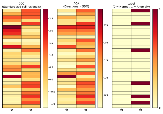
Figure 18: Features obtained by DDC (left) and ACA (middle) to detect and explain anomalies compared to true labels (right).

$\gamma=0.8$	$\gamma=0.9$
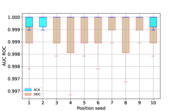
$\gamma=1$	$\gamma=1.5$

Figure 19: AUC computed using respective features for both methods DDC and ACA in the setting where they have approximately equal performance; 50 simulations are performed for each of $10$ position seed values.

3.2 Setting delivering different performance

This second setting is discussed in Section 4.2 where anomalies are placed in the same way as before with $X_{2}$ being more ‘responsible’ for abnormality than $X_{1}$. This results in better performance for ACA. The setting is explained in Figure 20 and we display the features in Figure 21 obtained with DDC and ACA which are used to compute AUR indicated in Figure 10.

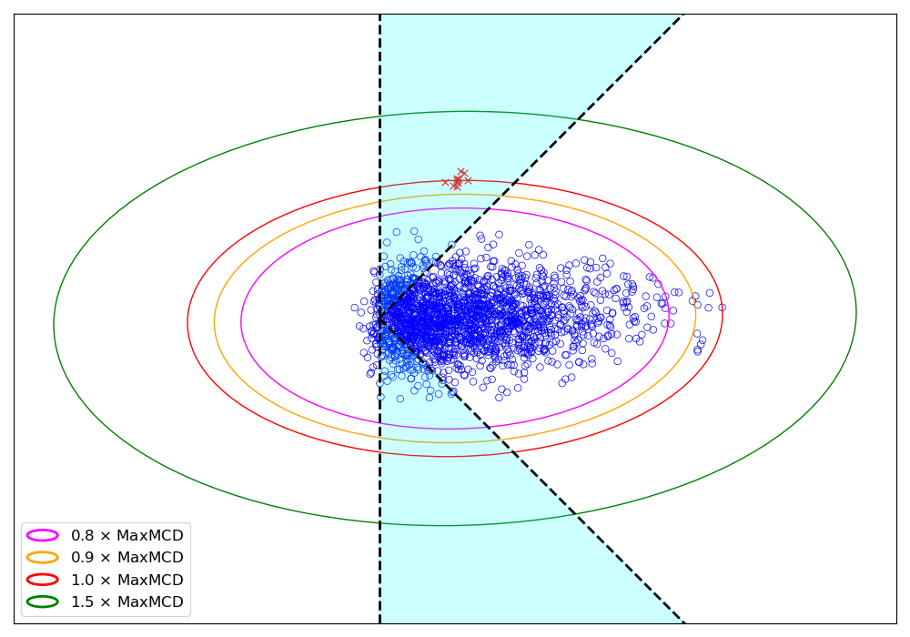
Figure 20: Second setting for comparison between ACA and DDC. Two symmetric areas of $45^{\circ}$ from the ordinate in cyan, in which anomalies are placed at various Mahalanobis distances (represented by colored ellipses) from the center. Scatter for the Mahalanobis distance is estimated using minimum covariance determinant (Rousseeuw and Driessen, 1999) and location is in $(0,0)^{\top}$.

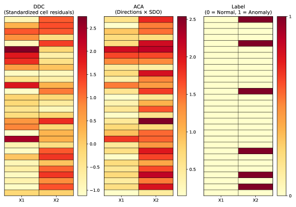
Figure 21: Features obtained by DDC (left) and ACA (middle) to detect and explain anomalies compared to true labels (right).

4 Real data

Following data sets are explored in the same manner as in Section 5. Obtained visualisations and explanations are competitive to those delivered by the methods of the state of the art. We also add tables with variables’ contributions for components for ACA, PCA, robPCA and ICA to interpret anomalies location.

Dataset	$\boldsymbol{n}$	$\boldsymbol{d}$	# Anomaly	% Anomaly	Category
Breastw	683	9	239	34.99	Healthcare
Vowels	1456	12	50	3.43	Linguistics
WDBC	367	30	10	2.72	Healthcare
Wine	129	13	10	7.75	Chemistry

Table 9: Data sets description

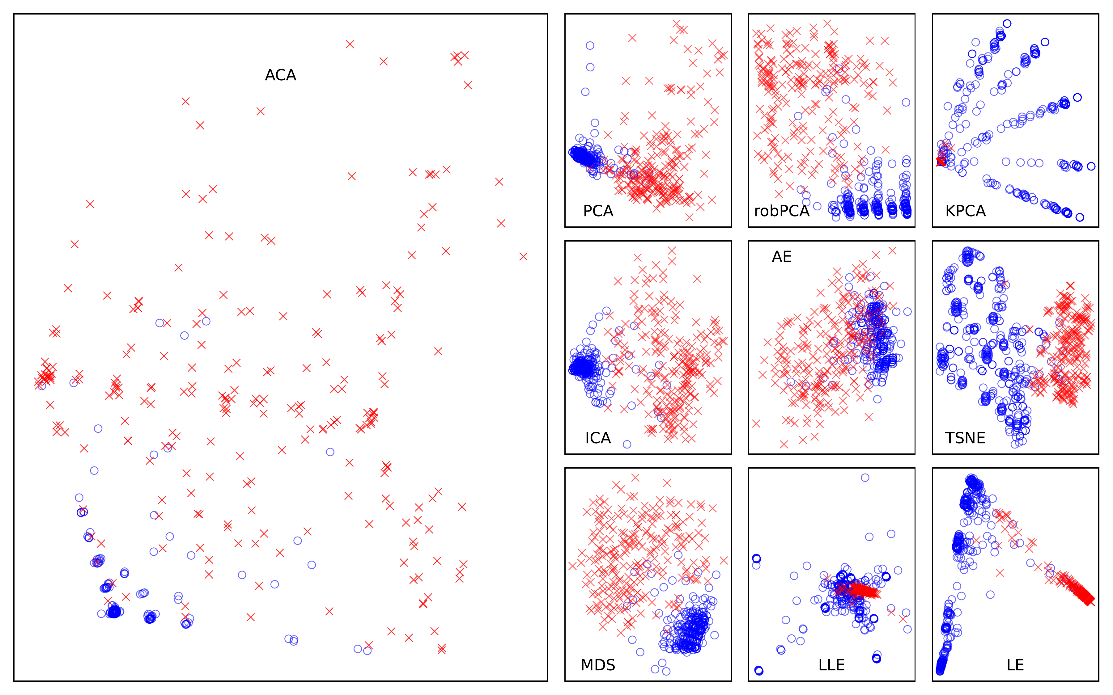
Figure 22: Breastw data set

	Breastw data set
	PCA		robPCA		ICA		ACA
	PC1	PC2	robPC1	robPC2	IC1	IC2	AC1	AC2
Var1	2 (13%)	9 (47%)	1 (80%)	6 (51%)	6 (32%)	6 (33%)	8 (62%)	9 (54%)
Var2	3 (13%)	6 (14%)	4 (10%)	5 (18%)	4 (14%)	8 (22%)	9 (18%)	6 (34%)
Var3	7 (12%)	7 (12%)	3 (4%)	3 (14%)	1 (12%)	2 (11%)	6 (14%)	8 (8%)
Var4	5 (11%)	5 (9%)	5 (2%)	4 (8%)	3 (11%)	5 (10%)	5 (3%)	4 (2%)
Var5	8 (11%)	1 (7%)	2 (2%)	7 (4%)	7 (11%)	9 (9%)	7 (1%)	2 (1%)
Var6	6 (11%)	3 (4%)	6 (1%)	1 (3%)	2 (10%)	3 (8%)	2 (1%)	1 (0%)
Var7	4 (11%)	4 (3%)	7 (0%)	2 (1%)	5 (5%)	4 (3%)	3 (1%)	7 (0%)
Var8	1 (10%)	2 (2%)	9 (0%)	8 (1%)	8 (3%)	1 (2%)	4 (0%)	3 (0%)
Var9	9 (8%)	8 (2%)	8 (0%)	9 (0%)	9 (1%)	7 (1%)	1 (0%)	5 (0%)

Table 10: Most important variables for every method applied to Breastw data set.

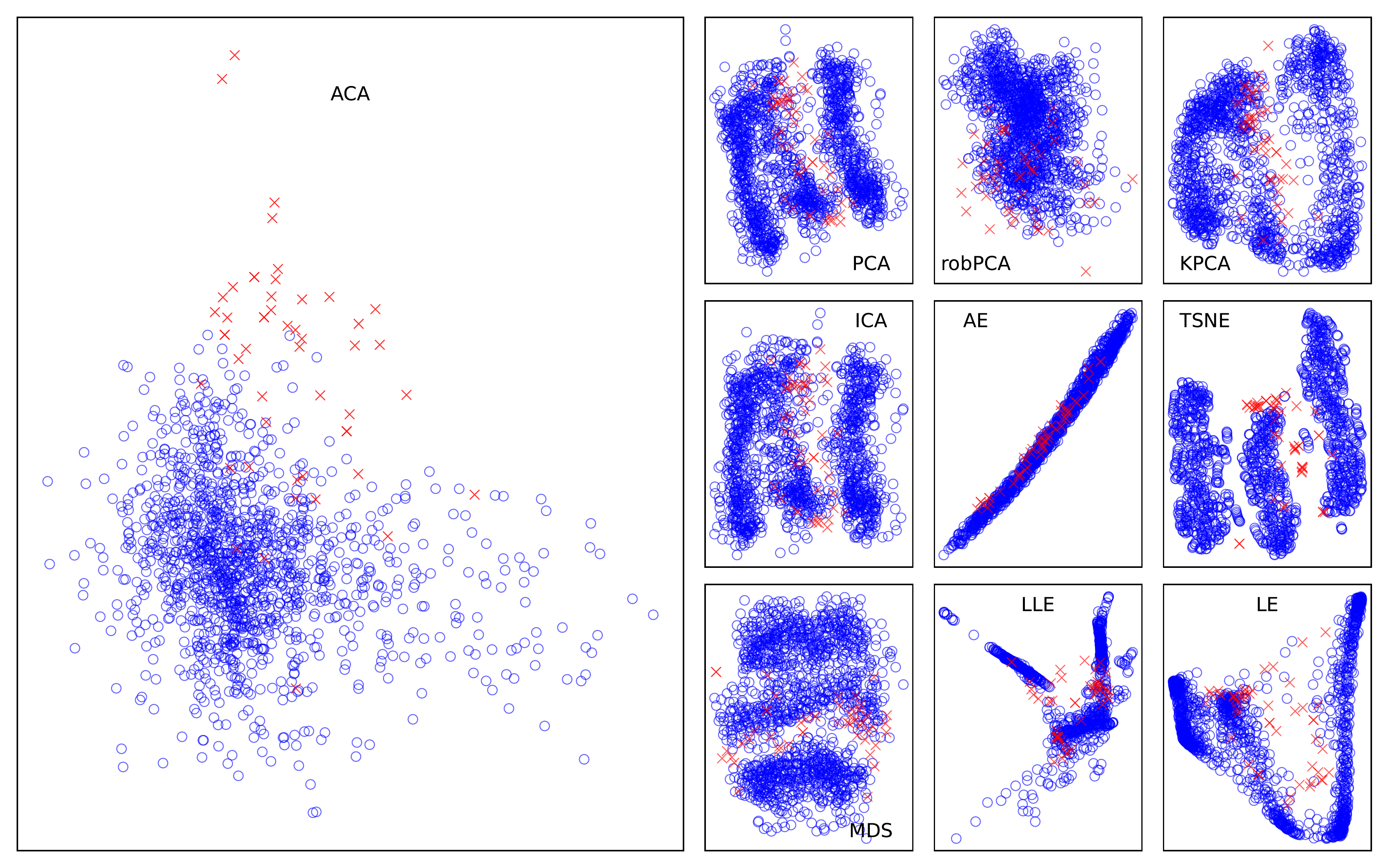
Figure 23: Vowels data set

	Vowels data set
	PCA		robPCA		ICA		ACA
	PC1	PC2	robPC1	robPC2	IC1	IC2	AC1	AC2
Var1	2 (15%)	5 (15%)	5 (29%)	9 (20%)	9 (16%)	4 (15%)	3 (15%)	1 (28%)
Var2	3 (15%)	4 (14%)	2 (15%)	10 (14%)	3 (15%)	8 (14%)	4 (13%)	7 (13%)
Var3	9 (14%)	8 (14%)	6 (9%)	6 (13%)	2 (15%)	5 (12%)	11 (11%)	11 (11%)
Var4	11 (9%)	1 (13%)	8 (9%)	12 (10%)	5 (13%)	6 (12%)	1 (10%)	9 (9%)
Var5	5 (8%)	7 (12%)	7 (8%)	4 (9%)	1 (11%)	1 (11%)	10 (10%)	4 (9%)
Var6	12 (8%)	6 (11%)	3 (7%)	1 (8%)	7 (7%)	11 (10%)	8 (8%)	3 (7%)
Var7	4 (8%)	11 (8%)	1 (6%)	2 (6%)	12 (6%)	7 (10%)	9 (8%)	12 (7%)
Var8	1 (7%)	12 (6%)	12 (6%)	3 (6%)	11 (6%)	12 (8%)	5 (6%)	8 (7%)
Var9	10 (4%)	9 (3%)	9 (5%)	8 (6%)	10 (5%)	2 (4%)	12 (6%)	2 (4%)
Var10	8 (4%)	10 (2%)	10 (3%)	11 (5%)	4 (4%)	3 (2%)	7 (5%)	10 (3%)

Table 11: Most important variables for every method applied to Vowels data set.

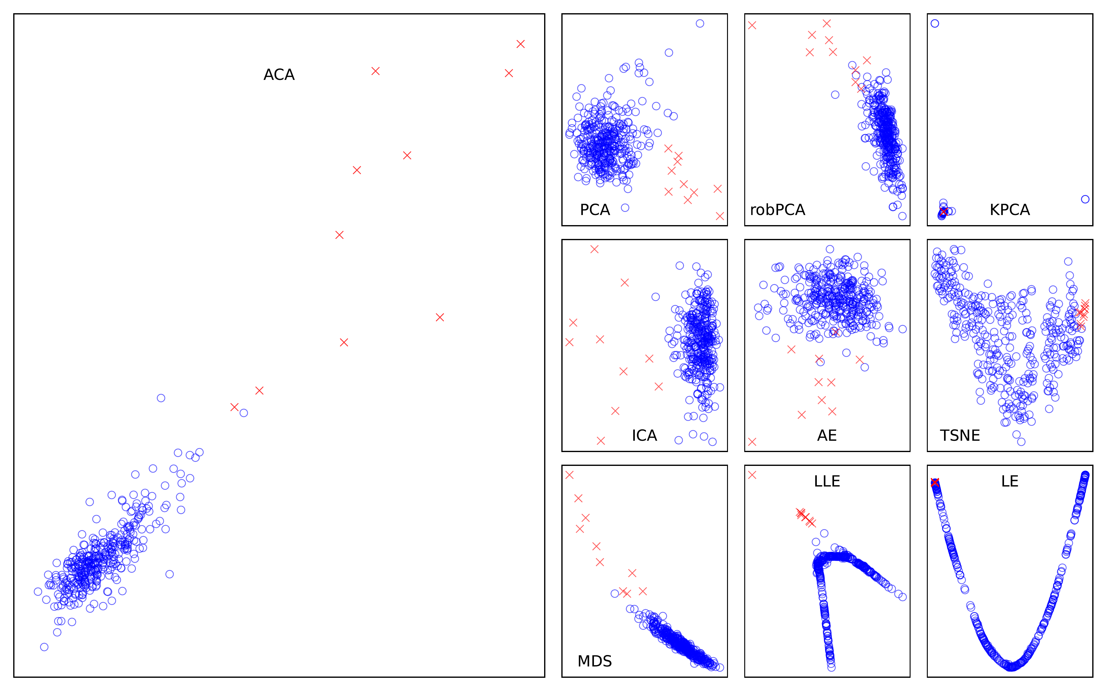
Figure 24: WDBC data set

	WDBC data set
	PCA		robPCA		ICA		ACA
	PC1	PC2	robPC1	robPC2	IC1	IC2	AC1	AC2
Var1	8 (6%)	10 (7%)	13 (22%)	6 (48%)	4 (43%)	4 (52%)	4 (8%)	16 (8%)
Var2	7 (6%)	1 (6%)	12 (12%)	3 (35%)	24 (40%)	24 (30%)	24 (8%)	19 (8%)
Var3	28 (6%)	4 (6%)	9 (12%)	8 (6%)	14 (7%)	14 (7%)	6 (7%)	23 (7%)
Var4	6 (5%)	21 (6%)	15 (10%)	7 (3%)	3 (5%)	3 (6%)	13 (7%)	28 (6%)
Var5	27 (5%)	3 (6%)	14 (8%)	9 (2%)	22 (2%)	22 (2%)	16 (6%)	30 (6%)
Var6	26 (5%)	24 (6%)	17 (5%)	5 (1%)	2 (1%)	2 (1%)	7 (6%)	20 (5%)
Var7	23 (5%)	23 (6%)	8 (4%)	11 (1%)	1 (1%)	1 (1%)	26 (5%)	10 (5%)
Var8	18 (4%)	15 (5%)	11 (4%)	4 (1%)	23 (1%)	13 (1%)	30 (5%)	12 (5%)
Var9	24 (4%)	20 (5%)	18 (3%)	2 (1%)	13 (1%)	23 (0%)	9 (4%)	25 (5%)
Var10	14 (4%)	30 (5%)	10 (3%)	10 (1%)	11 (0%)	21 (0%)	19 (4%)	15 (5%)

Table 12: Most important variables for every method applied to WDBC data set.

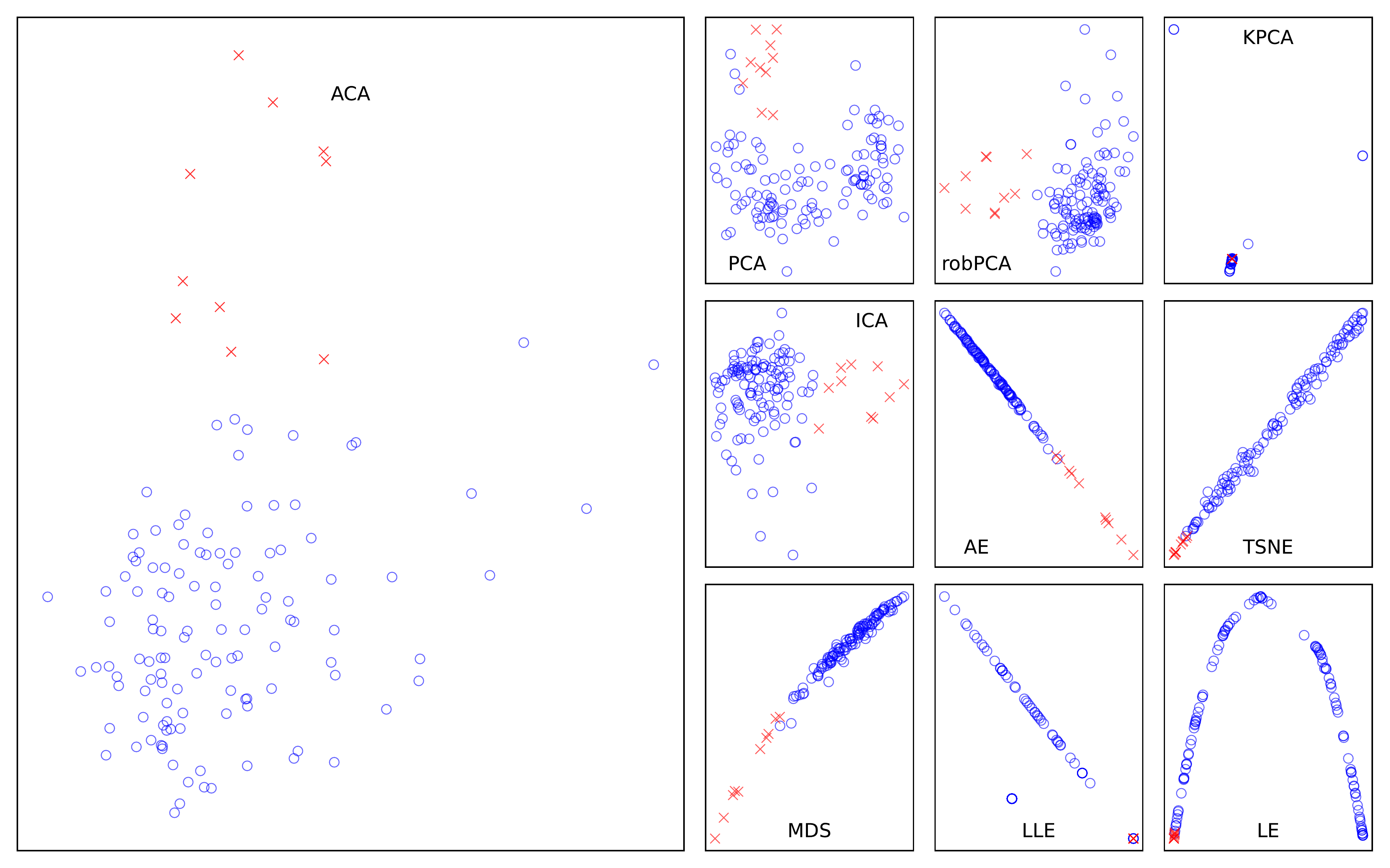
Figure 25: Wine data set

	Wine data set
	PCA		robPCA		ICA		ACA
	PC1	PC2	robPC1	robPC2	IC1	IC2	AC1	AC2
Var1	12 (13%)	13 (16%)	7 (62%)	5 (46%)	5 (70%)	5 (93%)	5 (34%)	9 (16%)
Var2	7 (13%)	5 (14%)	4 (12%)	6 (16%)	13 (26%)	4 (2%)	4 (17%)	3 (14%)
Var3	11 (11%)	1 (13%)	9 (9%)	4 (12%)	4 (2%)	13 (2%)	2 (10%)	13 (14%)
Var4	6 (11%)	3 (11%)	5 (8%)	7 (7%)	10 (1%)	10 (1%)	11 (10%)	8 (13%)
Var5	10 (10%)	10 (11%)	12 (2%)	3 (6%)	9 (1%)	9 (1%)	10 (7%)	12 (12%)
Var6	2 (9%)	6 (9%)	6 (2%)	9 (3%)	12 (0%)	12 (1%)	1 (5%)	11 (9%)
Var7	9 (9%)	9 (8%)	10 (2%)	11 (2%)	3 (0%)	3 (0%)	12 (5%)	5 (8%)
Var8	8 (8%)	7 (7%)	13 (1%)	12 (2%)	1 (0%)	1 (0%)	7 (5%)	2 (4%)
Var9	1 (7%)	8 (4%)	8 (1%)	10 (2%)	8 (0%)	8 (0%)	8 (5%)	7 (3%)
Var10	3 (4%)	11 (3%)	2 (1%)	8 (1%)	6 (0%)	6 (0%)	9 (1%)	1 (3%)

Table 13: Most important variables for every method applied to Wine data set.

References

- Agostinelli et al. (2015) C. Agostinelli, A. Leung, V. J. Yohai, and R. H. Zamar. Robust estimation of multivariate location and scatter in the presence of cellwise and casewise contamination. TEST, 24:441–461, 2015.
- Ahmed et al. (2016) M. Ahmed, A. N. Mahmood, and M. R. Islam. A survey of anomaly detection techniques in financial domain. Future Generation Computer Systems, 55:278–288, 2016.
- Anowar et al. (2021) F. Anowar, S. Sadaoui, and B. Selim. Conceptual and empirical comparison of dimensionality reduction algorithms (pca, kpca, lda, mds, svd, lle, isomap, le, ica, t-sne). Computer Science Review, 40:100378, 2021.
- Azzalini and Capitanio (1999) A. Azzalini and A. Capitanio. Statistical applications of the multivariate skew normal distribution. Journal of the Royal Statistical Society: Series B (Statistical Methodology), 61(3):579–602, 1999.
- Barredo Arrieta et al. (2020) A. Barredo Arrieta, N. Díaz-Rodríguez, J. Del Ser, A. Bennetot, S. Tabik, A. Barbado, S. Garcia, S. Gil-Lopez, D. Molina, R. Benjamins, R. Chatila, and F. Herrera. Explainable artificial intelligence (xai): Concepts, taxonomies, opportunities and challenges toward responsible ai. Information Fusion, 58:82–115, 2020.
- Bateni and Dalalyan (2020) A.-H. Bateni and A. S. Dalalyan. Confidence regions and minimax rates in outlier-robust estimation on the probability simplex. Electronic Journal of Statistics, 14:2653–2677, 2020.
- Belkin and Niyogi (2003) M. Belkin and P. Niyogi. Laplacian eigenmaps for dimensionality reduction and data representation. Neural Computation, 15(6):1373–1396, 2003.
- Carletti et al. (2023) M. Carletti, M. Terzi, and G. A. Susto. Interpretable anomaly detection with diffi: Depth-based feature importance of isolation forest. Engineering Applications of Artificial Intelligence, 119:105730, 2023.
- Chandola et al. (2009) V. Chandola, A. Banerjee, and V. Kumar. Anomaly detection: A survey. ACM Computing Surveys, 41(3), 2009.
- Comon (1992) P. Comon. Independent component analysis. In J.L.Lacoume, editor, Higher-Order Statistics, pages 29–38. Elsevier, 1992.
- Cox and Cox (2008) M. A. A. Cox and T. F. Cox. Multidimensional Scaling, pages 315–347. Springer Berlin Heidelberg, 2008.
- Diakonikolas et al. (2016) I. Diakonikolas, G. Kamath, D. M. Kane, J. Li, A. Moitra, and A. Stewart. Robust estimators in high dimensions without the computational intractability. In IEEE 57th Annual Symposium on Foundations of Computer Science (FOCS), pages 655–664. IEEE, 2016.
- Donoho (1982) D. L. Donoho. Breakdown properties of multivariate location estimators. PhD thesis, Dept. Statistics, Harvard University, Boston, 1982.
- Doshi-Velez and Kim (2017) F. Doshi-Velez and B. Kim. Towards a rigorous science of interpretable machine learning. arXiv preprint arXiv:1702.08608, 2017.
- Dyckerhoff (2004) R. Dyckerhoff. Data depths satisfying the projection property. Allgemeines Statistisches Archiv, 88:163–190, 2004.
- Dyckerhoff et al. (2021) R. Dyckerhoff, P. Mozharovskyi, and S. Nagy. Approximate computation of projection depths. Computational Statistics & Data Analysis, 157:107166, 2021.
- Görnitz et al. (2013) N. Görnitz, M. Kloft, K. Rieck, and U. Brefeld. Toward supervised anomaly detection. Journal of Artificial Intelligence Research, 46:235–262, 2013.
- Hotelling (1933) H. Hotelling. Analysis of a complex of statistical variables into principal components. Journal of Educational Psychology, 24:417–441, 1933.
- Huber (1964) P. J. Huber. Robust estimation of a location parameter. The Annals of Mathematical Statistics, (35):73–101, 1964.
- Huber (1965) P. J. Huber. A robust version of the probability ratio test. The Annals of Mathematical Statistics, (36):1753–1758, 1965.
- Hubert et al. (2005) M. Hubert, P. J. Rousseeuw, and K. V. Branden. Robpca: A new approach to robust principal component analysis. Technometrics, 47(1):64–79, 2005.
- Kim et al. (2018) B. Kim, M. Wattenberg, J. Gilmer, C. Cai, J. Wexler, F. Viegas, and R. Sayres. Interpretability beyond feature attribution: Quantitative testing with concept activation vectors (TCAV). In J. Dy and A. Krause, editors, Proceedings of the 35th International Conference on Machine Learning, volume 80 of Proceedings of Machine Learning Research, pages 2668–2677. PMLR, 2018.
- Kotík and Hlubinka (2017) L. Kotík and D. Hlubinka. A weighted localization of halfspace depth and its properties. Journal of Multivariate Analysis, 157:53–69, 2017.
- Lee and Seung (1999) D. D. Lee and H. S. Seung. Learning the parts of objects by non-negative matrix factorization. Nature, 401(6755):788–791, 1999.
- Li et al. (2023) Z. Li, Y. Zhu, and M. Van Leeuwen. A survey on explainable anomaly detection. ACM Transactions on Knowledge Discovery from Data, 18(1), 2023.
- Liu et al. (2008) F. T. Liu, K. M. Ting, and Z.-H. Zhou. Isolation forest. In 2008 eighth ieee international conference on data mining, pages 413–422. IEEE, 2008.
- Lopuhaa and Rousseeuw (1991) H. P. Lopuhaa and P. J. Rousseeuw. Breakdown points of affine equivariant estimators of multivariate location and covariance matrices. The Annals of Statistics, 19(1):229–248, 1991.
- Mosler and Mozharovskyi (2022) K. Mosler and P. Mozharovskyi. Choosing among notions of multivariate depth statistics. Statistical Science, 37(3):348–368, 2022.
- Murdoch et al. (2019) W. J. Murdoch, C. Singh, K. Kumbier, R. Abbasi-Asl, and B. Yu. Definitions, methods, and applications in interpretable machine learning. Proceedings of the National Academy of Sciences, 116(44):22071–22080, 2019.
- Nagy et al. (2020) S. Nagy, R. Dyckerhoff, and P. Mozharovskyi. Uniform convergence rates for the approximated halfspace and projection depth. Electronic Journal of Statistics, 14(2):3939 – 3975, 2020.
- Parekh et al. (2021) J. Parekh, P. Mozharovskyi, and F. d’Alché Buc. A framework to learn with interpretation. Advances in Neural Information Processing Systems, 34:24273–24285, 2021.
- Pearson (1901) K. Pearson. On lines and planes of closest fit to systems of points in space. The London, Edinburgh, and Dublin Philosophical Magazine and Journal of Science, 2(11):559–572, 1901.
- Rayana (2016) S. Rayana. ODDS library. https://odds.cs.stonybrook.edu, 2016. Stony Brook University, Department of Computer Sciences.