A Hamiltonian for 1:1 Rotational Secondary Resonances, and Application to Small Satellites of Saturn and Jupiter

Abstract

In this work, we study the dynamics of rotation of the small satellites Methone and Aegaeon and revisit previous works on the rotation of Prometheus, Metis, and Amalthea. In all cases, the surfaces of section computed with the standard spin-orbit model reveal that the synchronous regime shares another large domain in the rotation phase space. We reproduce and apply the hamiltonian theory given in Wisdom (2004) to analytically characterize the detected structure as being a secondary resonance where the period of oscillations around the synchronism is similar to the orbital period. Being that the current rotational states of this sort of satellite should be synchronous (Thomas and Helfenstein 2020), our results can be taken into account in evolutionary studies of their rotation.

1 Introduction

Consider the rotation of a rigid and homogeneous satellite orbiting a punctual planet in the case the satellite rotates around a single axis corresponding to its largest moment of inertia. The mutual perturbations between the bodies belonging to multiple systems or due to the non-sphericity of the secondary are neglected in this work, such that the motion of the system is governed by the laws of the two-body problem (Goldreich and Peale 1966).

A hamiltonian for the sort of problem is given by:

$$H(\theta,p,t)=\frac{p^{2}}{2C}-\frac{\epsilon^{2}n^{2}C}{4}\left[\frac{\textsf{a}}{r(t)}\right]^{3}\cos{2[\theta-f(t)]},$$ (1)

where $\theta$ is an angle of rotation of the satellite measured from an inertial line; $p=C\dot{\theta}$ is the angular momentum of rotation around the $z-$axis assumed to be perpendicular to the orbital plane, and $\dot{\theta}$ is the angular velocity of rotation. $A<B<C$ are the moments of inertia around the principal axis of the satellite around the $x$, $y$, $z$, respectively; a, $e$, $f(t)$, $r(t)=\frac{\textsf{a}(1-e^{2})}{1+e\cos f(t)}$, $n$ are the semi-major axis, orbital eccentricity, true anomaly, planet-satellite distance, and the mean-motion of the satellite, respectively.

It is well known that the dynamics of rotation of mid-sized satellites of the outer planets and the Moon are mainly characterized by synchronous orbit-rotation resonances (see Peale 1977, Melnikov and Shevchenko 2022). The exact synchronism occurs when the angular velocity of rotation of the satellite equals its mean motion, $n$. In practice, the synchronous resonance of the satellites is characterized by the physical libration of the angle $\Psi(t)=\theta(t)-f(t)$. $\Psi$ contains all main components of the spin-orbit perturbations, namely, the optical, free, and forced librations (see Callegari and Ribeiro 2015, and references therein). In the case of a small amplitude of libration of $\Psi$ and small orbital eccentricity of the satellite, the physics of the synchronous resonance can be interpreted by an analog of the forced harmonic oscillator (see Murray and Dermott 1999). Suppose also to model the shape of the satellite with a Roche ellipsoid with semi-axes $a$, $b$, and $c$ in the $x$, $y$, $z$ directions, respectively; in this case, $a>b>c$ (see Callegari and Rodríguez 2013, and references therein). Denote the free frequency by $\omega$ (which corresponds to the frequency of the oscillator in the harmonic approximation). The average linear theory of synchronous resonance predicts that the ratio of the free and orbital frequencies $\frac{\omega}{n}$ is given by:

$$\epsilon\equiv\frac{\omega}{n}=\left(3\frac{B-A}{C}\right)^{1/2}=\left[3\left(\frac{a^{2}-b^{2}}{a^{2}+b^{2}}\right)\right]^{1/2}.$$ (2)

Thus, when $\epsilon$ is a rational number, an inner resonance can rise due to the commensurability between $n$ and $\omega$. We have therefore a definition for secondary resonance within the synchronous regime (in the case of a synchronous rotating satellite). The approximation of a simple oscillator is no longer enough to describe the rotational dynamics in this situation, and additional analyses (e.g. perturbation theory) are necessary to describe the dynamics of rotation in more detail.

The case of the Saturnian satellite Enceladus studied in Wisdom (2004) is a good example to illustrate the dynamics of secondary resonances. Under the hypothesis of a homogeneous body, and based on Voyager spacecraft data, the dimensions of Enceladus are $a=256.3\pm 0.3$ km, $b=247.3\pm 0.3$ km, $c=244.6\pm 0.3$ km (Dermott and Thomas 1994). From Equation (2) we obtain $\epsilon\sim 0.327$, a value close to $\frac{1}{3}$, so that Wisdom conjectured if Enceladus would be currently rotating close to the $\frac{\omega}{n}=\frac{1}{3}$ secondary resonance.

While it is certain that current rotational states of all mid-sized satellites of the giant planets are characterized by synchronous resonance, the same is not necessarily true for all other smaller secondary companions having mean-radius of the order of a few dozens kilometer. Several of them are irregularly shaped, and due to this, $\epsilon$ is large. Let us consider the case of Amalthea (J15), a member of the inner group of Jupiter satellites composed of Metis, Adrastea, Amalthea, and Thebe. Amalthea is significantly out of round with dimensions $a\times b\times c$ of the order of $\sim$ $125\times\sim 73\times\sim 64$ such that $\epsilon\sim 1.214$. These values are given after analyses of Galileo tour in Jupiter system; Thomas et al. 1998 (see also Pashkevich et al. 2021, and references therein). The phase space of rotation of Amalthea shows the existence of two resonant modes within the synchronism. They denote these modes by “$\alpha$-resonance” and “$\beta$-resonance”, and named this property of the synchronous regime by the “Amalthea effect”. The existence of such kind of “bifurcation” inside the synchronous domain leads to questioning and discussions on topics related to the evolution of rotation and the true current equilibrium configuration of the satellite (see discussions in Melnikov and Shevchenko 2002, and references therein). Another body with similar rotational properties of the phase space is the Prometheus (Melnikov and Shevchenko 2008), from Saturn, a close-in with a mean radius of 42.8 km (see Table 1).

Table 1: Selected physical and orbital parameters of the satellites studied in this work. In the case of Saturn,
the values of the orbital eccentricities correspond to the maximum geometric values (Callegari et al. 2021;
Ceccatto et al. 2021, Callegari and Rodríguez 2023).

	Methonea	Aegaeona	Prometheusa	Amaltheab	Metisb
semi-major axis (km)	194,707	168,031	140,029	181,400	128,000
eccentricity	0.0014	0.0005	0.00226	0.0031	0.0002
dimensions (km)	$1.94\times$	$0.7\times$	$68.5\times$	$125\times$	$30\times$
	$1.29\times$	$0.25\times$	$40.5\times$	$73\times$	$20\times$
	1.21	0.20	28.1	64	17
$\epsilon$	1.077	1.5236	1.1717	1.2140	1.074

$(^{a})$ Thomas and Helfenstein 2020; $(^{b})$ Thomas et al. 1998; Pashkevich et al. 2021

The objects we study in this project belong to another class of even smaller inner satellites of the Jovian planets having mean diameters of a few kilometers or even less. We consider in this work the Saturnian satellites Methone (S/2004 S 1) and Aegaeon (S/2008 S 1) discovered by the Cassini spacecraft in 2004 (Porco 2004) and 2008 (Porco 2009), respectively. Similarly to Amalthea and Prometheus, their phase spaces also display the co-existence of the $\alpha$ and $\beta$-“resonances”. Methone, jointly with Aegaeon and Pallene is classified as ellipsoidal-like satellites. We will focus next and throughout the paper on the case of Methone, and at the end of the paper, similar results will be shown and discussed for Aegaeon and Prometheus. The cases of Amalthea and Metis will also be revisited given the theory developed here.

To investigate the rotation of Methone, we apply the standard model of spin-orbit resonance. We utilize the Everhart (1985) algorithm to solve numerically the rotation differential equations derived from hamiltonian (1). The full equation is non-autonomous such that, at first, we compute the surfaces of section (hereafter denoted by SOS), a practical procedure often applied in studies of rotation after Wisdom et al. (1984). In this technique, the pair of generalized variables $(\theta,\dot{\theta}/n)$ is plotted every time the satellite passes through the pericenter of its orbit. Figure 1a) shows the SOS for Methone in the vicinity of the synchronous domain. The fixed points of the $\alpha$ and $\beta$-“resonances” are indicated by vertical arrows. Note that the regimes are separated by a new separatrix (red curve in Fig. 1a)), while they are encompassed by a thin chaotic layer associated to the synchronous domain.

The main goal of this work is to investigate the nature of the $\alpha$ and the $\beta$-regimes in the case of the satellite Methone. Both share the synchronous domain, so it is worth giving a cinematic description of the rotation of clones of Methone departing from initial conditions very close to their fixed points to identify their differences. Figs. 1(b,c) show the time variations of $\frac{\dot{\theta}}{n}$ and $\Psi=\theta-f$ corresponding to the $\alpha$ and $\beta$-regimes, respectively. The initial conditions are $\theta_{0}=0$ in both cases and $\frac{\dot{\theta}(0)}{n}=1$, $\frac{\dot{\theta}(0)}{n}=0.45$ in b) and c), respectively.

In the case of the $\beta$-regime (Fig. 1b)), $\Psi$ oscillates around zero with amplitude of $\sim 0.04$ radian (or $\sim 2$ degree) and $\frac{\dot{\theta}}{n}$ oscillates with amplitude of $\sim 0.036$. In both variables there is a “long-term” mode resulting from close values of the fundamental frequencies $n$ and $\omega$. In fact, from Equation (2) we have $\omega=n\epsilon$ and $\epsilon\sim 1.077$. Denoting by $T$, $P$, $T_{\omega}$ the periods of the beating, the orbital period, and the period of the free libration, we obtain $T\sim 13.2$ day from the relation $\frac{1}{T}=\frac{1}{P}-\frac{1}{T_{\omega}}$ considering $P\sim 1.014$ day and $T_{\omega}=P/\epsilon$.

In the case of the $\alpha$-regime (Fig. 1c)), $\Psi$ oscillates around zero with amplitude of $\sim 0.5$ radian (or $\sim 29$ degree). $\frac{\dot{\theta}}{n}$ oscillates around the unit with amplitude of $\sim 0.5$ such that at the minima (indicated by black points in Fig. 1(b)), the satellite is always located at the pericenter of its orbit (open circles in Fig. 1(b)). Thus, due to this relatively large amplitude of oscillation of $\frac{\dot{\theta}}{n}$, the SOS displays $\frac{\dot{\theta}}{n}\sim 0.45$, the same as that of the initial value.

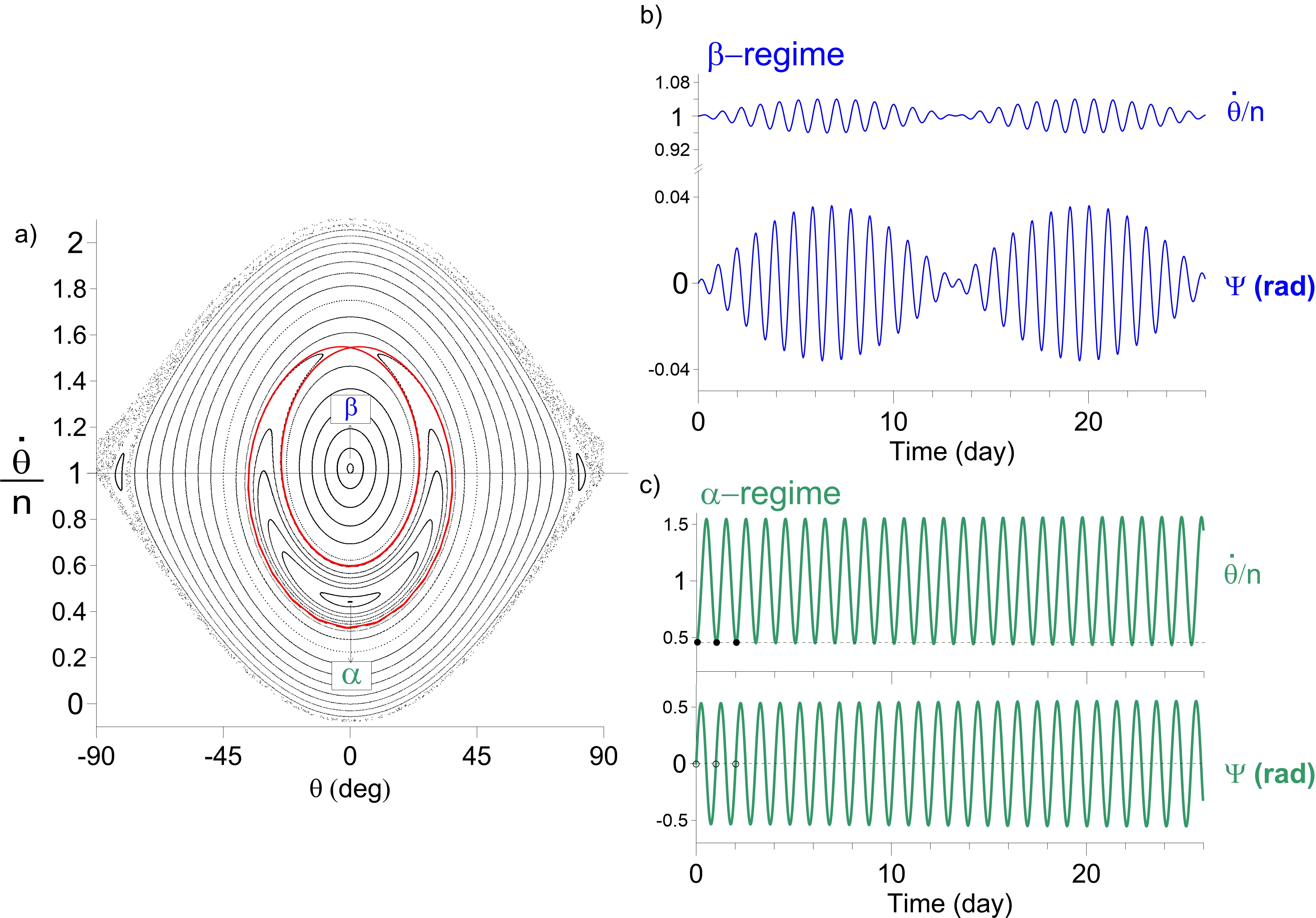
Figure 1: (a) Surfaces of section of solutions of the model (1) applied to the satellite Methone. Each orbit has been integrated for 500 orbital periods of the satellite. The sections (projections) are made at each orbital revolution, and all the time the true anomaly of the satellite reaches $f=0$. The $x$ and $y$-axes are the (projected) rotation angle ($\theta$) around the axis of the largest moment of inertia and the ratio of the angular velocity of rotation and the mean motion, $\frac{\dot{\theta}}{n}$. The vertical arrows indicate the fixed points associated with the $\alpha$ and $\beta$ regimes of rotation. The numerical values of the parameters of the model adopted in this work which is necessary in the numerical solution are: $\textsf{a}=194,707.6$ km, $e=0.0014$, $a=1.94$ km, $b=1.29$ km (see Section 1 for definitions). (b,c) Time variations of $\frac{\dot{\theta}(t)}{n}$, $\Psi(t)=\theta(t)-f(t)$ for two trajectories within the domains of the $\alpha$ and $\beta$-regimes, respectively. $\theta_{0}=0$ in both cases and $\frac{\dot{\theta}(0)}{n}=1$, $\frac{\dot{\theta}(0)}{n}=0.45$ in b) and c), respectively. The horizontal dashed lines plotted in (c) guide the solutions close to the fixed points at the pericenter passage, while the horizontal line in (a) gives the straight $\frac{\dot{\theta}(t)}{n}=1$.

Since the Methone’s phase space of rotation displays additional structures within the synchronous regime, all discussion given above leads us to investigate the existence of secondary resonances. Accordin to the most recent analyses of data taken from Cassini measurements, Thomas and Helfenstein (2020) determined that the dimensions of Methone are $a=1.94\pm 0.02$ km, $b=1.29\pm 0.04$ km, $c=1.21\pm 0.02$ km so that $\epsilon\sim 1.077$. This value of $\epsilon$ is close to the unit so that we conjecture if a 1:1 secondary resonance of the type $\frac{\omega}{n}\sim\frac{1}{1}$ would explain the existence of $\alpha$ and $\beta$ structures within the synchronous domain. To prove the conjecture we return to the Wisdom’s (2004) paper. He developed a simple analytical model for spin-orbit problem in hamiltonian formalism aiming to explain the phase space of Enceladus in the close vicinity of the synchronous regime. Having in hand an expanded version of hamiltonian of Equation (1), he selected the correct terms and explained analytically the properties of the secondary $\frac{1}{3}$ resonance. We follow his steps and reproduce its main results, and we choose those terms in hamiltonian which are proportional to the arguments containing the $\frac{1}{1}$ secondary resonance. By adopting a similar methodology given in Wisdom (2004), we successfully explain the co-existence of the $\alpha$ and $\beta$-regimes in synchronous resonance by comparing the SOS with level curves of the constructed hamiltonian.

The presentation of the results of this paper is divided as follows. In Section 2, we deduce the expanded hamiltonian developed in Wisdom (2004) in detail, showing the terms of the hamiltonian explicitly (that ones related to equation 20 of the referred paper); some extensions of Wisdom’s model are also given. In Sections 3.1 and 3.2, we show exactly how the perturbed hamiltonian can give rise to the secondary resonances and write the hamiltonian for the $\frac{1}{1}$ secondary resonance. The level curves applied in the case of Methone are shown in Section 3.3. Analytical estimative of the bifurcations of the level curves are also provided. In Section 4 we analyze the cases of Aegaeon and Prometheus, and Section 5 is devoted to conclusions and more general discussion involving other satellites. Since the phase space of rotation of Methone, Aegaeon, Prometheus, Amalthea, Metis, and others share similar structures and properties within the synchronous regime, we are led to question their current states of rotation.

2 Expansion of the hamiltonian (1)

2.1 An integrable hamiltonian

The hamiltonian (1) is analogous to that one of a simple non-autonomous pendulum. An expanded version of the hamiltonian can be obtained resulting in a sum of autonomous-like pendulums. This can easily achieved after substituting in hamiltonian (1) the developed forms of $\left[\frac{\textsf{a}}{r(t)}\right]^{3}$, $\cos{2f(t)}$, $\sin{2f(t)}$:

$$\left[\frac{\textsf{a}}{r(t)}\right]^{3}\approx 1+3e\cos{nt}+\frac{3}{2}e^{2}(1+3\cos{2nt}),$$

$$\cos{2f(t)}\approx\cos{nt}+e(\cos{2nt}-1)+\frac{9}{8}e^{2}(\cos{3nt}-\cos{nt}),$$ (3)

$$\sin{2f(t)}\approx\sin{nt}+e\sin{2nt}+\frac{1}{8}e^{2}(9\sin{3nt}-7\sin{nt}).$$

We have:

$$H(\theta,p,t)=\frac{p^{2}}{2C} - \frac{\epsilon^{2}n^{2}C}{4}\left(+\frac{17}{2}e^{2}\right)\cos{(2\theta-4nt)}$$ (4)

$$- \frac{\epsilon^{2}n^{2}C}{4}\left(+\frac{7}{2}e\right)\cos{(2\theta-3nt)}$$

$$- \frac{\epsilon^{2}n^{2}C}{4}\left(1-\frac{5}{2}e^{2}\right)\cos{2(\theta-nt)}$$

$$- \frac{\epsilon^{2}n^{2}C}{4}\left(-\frac{1}{2}e\right)\cos{(2\theta-nt)}+\ldots.$$

Each term in the right side of (4) proportional to $\epsilon^{2}$ can be considered a distinct disturbing resonance associated to the commensurabilities $\dot{\theta}=2n$, $\dot{\theta}=\frac{3}{2}n$, $\dot{\theta}=n$ and $\dot{\theta}=\frac{n}{2}$, defining therefore the 2:1, 3:2, 1:1 (synchronous), and the 1:2 spin-orbit resonant states.

We can isolate a single resonance after applying the average principle (see footnote 1) and we can note that, whatever resonance, the resulting hamiltonian is always analogous to a simple non-autonomous pendulum. Canonical transformations can make each of the resonances given in Equation (4) locally integrable. For instance, consider the synchronous resonance and define $H_{0}$ by:

$$H_{0}(\theta,p,t)=\frac{p^{2}}{2C}-\frac{\epsilon^{2}n^{2}C}{4}\left(1-\frac{5}{2}e^{2}\right)\cos{2(\theta-nt)}.$$ (5)

Given the canonical transformation:

$$\phi = \theta-nt$$ (6)

$$\Phi = p-nC,$$

the new $H^{\prime}_{0}$ is given by:

$$H^{\prime}_{0}(\phi,\Phi,-) = -n\Phi+\frac{(\Phi+nC)^{2}}{2C}-\frac{\epsilon^{2}n^{2}C}{4}\cos{2\phi}\Rightarrow$$ (7)

$$= \frac{\Phi^{2}}{2C}-\frac{\epsilon^{2}n^{2}C}{4}\cos{2\phi},$$

where the term $-n\Phi$ comes from phase space extension (see Sussman and Wisdom 2001, Ferraz-Mello 2007). We have also neglected the term in $e^{2}$ since the orbital eccentricity of Methone is of the order of $10^{-3}$. Moreover, an irrelevant additive constant ($n^{2}C/2$) is not included in (7).

Thus, we have an integrable hamiltonian for the synchronous spin-orbit resonance. Since the hamiltonian (7) is analogous to the simple autonomous pendulum, we can use the equations of transformation to the action-angle variables developed to the simple pendulum which are given in several books. In this work, we consider only the libratory regime in the case of small oscillations.

The action variable $J$ is defined as being the area on the plane $(\phi,\Phi)$ divided by $2\pi$. The conjugated action $\psi$ varies linearly in time. The new hamiltonian depends only on the action and can be written as follows:

$$H^{{}^{\prime\prime}}_{0}(-,\tilde{J}) = \frac{\epsilon^{2}n^{2}C}{4}\left(-1+\tilde{J}-\frac{1}{16}\tilde{J}^{2}-\frac{1}{256}\tilde{J}^{3}+\ldots\right),$$ (8)

where

$$\tilde{J}=\frac{4J}{\epsilon nC},$$ (9)

such that

$$H^{{}^{\prime\prime}}_{0}(-,J)=-\frac{\epsilon^{2}n^{2}C}{4}+\epsilon nJ-\frac{1}{4C}J^{2}-\frac{1}{16\epsilon nC^{2}}J^{3}+\ldots.$$ (10)

The algebraic expression between the new variables $(\psi,J)$ and the old ones $(\phi,\Phi)$ is:

$$\sin{2\phi}\approx 2\phi=F_{1}\sin{\psi}+F_{3}\sin{3\psi}+\ldots,$$ (11)

where

$$F_{1} = \left(2\tilde{J}+\frac{1}{4}\tilde{J}^{2}+\frac{27}{512}\tilde{J}^{3}+\ldots\right)^{1/2}\approx\sqrt{\tilde{J}}+\frac{1}{16}(\sqrt{2\tilde{J}})^{3},$$ (12)

$$F_{3} = \frac{1}{192}\left[(2\tilde{J})^{3}\left(1+\frac{9}{16}\tilde{J}+\ldots\right)\right]^{1/2}\approx\frac{1}{192}(\sqrt{2\tilde{J}})^{3}+\ldots.$$ (13)

Equations (8)-(13) have been taken from Wisdom (2004). A proof of them can be obtained after applying the pendulum model to the hamiltonian (7) in the case of small oscillation approximation (see for instance appendix B.3 in Ferraz-Mello 2007).

2.2 Perturbation of the integrable hamiltonian

Let us consider now the time-dependent perturbations on the integrable part of the synchronous resonance of the hamiltonian such that

$$H^{\prime}(\phi,\Phi,t)=H^{\prime}_{0}+H^{\prime}_{1},$$ (14)

where $H^{\prime}_{0}$ is given in (7) and $H^{\prime}_{1}$ is the perturbation. We will include in $H^{\prime}_{1}$ the two neighboring resonances of the synchronous resonances, namely, 3:2 and 1:2 (see Equation (4)). In terms of old variables $(\phi,\Phi)$ we can obtain from (4) that:

$$H^{\prime}_{1}(\phi,\Phi,t)=-\frac{\epsilon^{2}n^{2}C}{4}\left[\frac{7e}{2}\cos{(2\phi-nt)}-\frac{e}{2}\cos{(2\phi+nt)}\right].$$ (15)

To write $H^{\prime}_{1}$ in terms of the action-angle variables we must consider the transformation equation (11). The algebraic manipulations can be much more simple considering the limit of small oscillations (Wisdom 2004). Thus, first write (13) as follows:

$$H^{\prime}_{1}(\phi,\Phi,t) = -\frac{\epsilon^{2}n^{2}C}{4}\left[\frac{7e}{2}(C_{2}\cos{nt}+S_{2}\sin{nt})-\frac{e}{2}(C_{2}\cos{nt}-S_{2}\sin{nt})\right],$$ (16)

$$C_{2} = \cos{2\phi}\approx 1-\frac{1}{2}(2\phi)^{2},S_{2}=\sin{2\phi}\approx 2\phi-\frac{1}{6}(2\phi)^{3}.$$ (17)

After substituting the expression (11) in (17) and the result in (16), we can obtain the perturbation $H^{\prime\prime}_{1}(\psi,J,t)$ as follows:

$$H^{\prime\prime}_{1}(\psi,J,t) = \epsilon^{2}n^{2}Ce\times$$ (18)

$$+ (3/16)F_{1}^{2}\cos{nt}+(3/16)F_{3}^{2}\cos{nt}-(3/4)\cos{nt}$$

$$- (1/2)F_{1}\cos{(nt-\psi)}$$

$$+ (1/16)F_{1}^{3}\cos{(nt-\psi)}$$

$$- (1/16)F_{1}^{2}F_{3}\cos{(nt-\psi)}$$

$$+ (1/8)F_{1}F_{3}^{2}\cos{(nt-\psi)}$$

$$- (3/32)F_{1}^{2}\cos{(nt-2\psi)}$$

$$+ (3/16)F_{1}F_{3}\cos{(nt-2\psi)}$$

$$+ (1/16)F_{3}^{3}\cos{(nt-3\psi)}$$

$$- (1/48)F_{1}^{3}\cos{(nt-3\psi)}$$

$$+ (1/8)F_{1}^{2}F_{3}\cos{(nt-3\psi)}$$

$$- (1/2)F_{3}\cos{(nt-3\psi)}$$

$$- (3/16)F_{1}F_{3}\cos{(nt-4\psi)}$$

$$+ (1/16)F_{1}F_{3}^{2}\cos{(nt-5\psi)}$$

$$- (1/16)F_{1}^{2}F_{3}\cos{(nt-5\psi)}$$

$$- (3/32)F_{3}^{2}\cos{(nt-6\psi)}$$

$$- (1/16)F_{1}F_{3}^{2}\cos{(nt-7\psi)}$$

$$- (1/48)F_{3}^{3}\cos{(nt-9\psi)}$$

$$- (1/16)F_{1}^{3}\cos{(nt+\psi)}$$

$$+ (1/2)F_{1}\cos{(nt+\psi)}$$

$$- (1/8)F_{1}F_{3}^{2}\cos{(nt+\psi)}$$

$$+ (1/16)F_{1}^{2}F_{3}\cos{(nt+\psi)}$$

$$+ (3/16)F_{1}F_{3}\cos{(nt+2\psi)}$$

$$- (3/32)F_{1}^{2}\cos{(nt+2\psi)}$$

$$- (1/16)F_{3}^{3}\cos{(nt+3\psi)}$$

$$+ (1/48)F_{1}^{3}\cos{(nt+3\psi)}$$

$$+ (1/2)F_{3}\cos{(nt+3\psi)}$$

$$- (1/8)F_{1}^{2}F_{3}\cos{(nt+3\psi)}$$

$$- (3/16)F_{1}F_{3}\cos{(nt+4\psi)}$$

$$+ (1/16)F_{1}^{2}F_{3}\cos{(nt+5\psi)}$$

$$- (1/16)F_{1}F_{3}^{2}\cos{(nt+5\psi)}$$

$$- (3/32)F_{3}^{2}\cos{(nt+6\psi)}$$

$$+ (1/16)F_{1}F_{3}^{2}\cos{(nt+7\psi)}$$

$$+ (1/48)F_{3}^{3}\cos{(nt+9\psi)}.$$

Note that at this step we are not utilizing the expanded versions of $F_{1}$ and $F_{3}$ given in the right side of Equations (12) and (13).

3 Perturbed hamiltonian and the rise of secondary resonances

3.1 The 1:1 secondary resonance

The transformation variable given in Equation (6), $\phi=\theta-nt$, consists of an approximation of the physical libration $\Psi$ valid for small eccentricity.

For small amplitude of oscillation, the frequency of the angle variable $\psi$ is the frequency of $\phi$ divided by $2\pi$. Thus, Equation (18) can be utilized to study several secondary resonances. Inspection of (18) shows the terms in arguments of the cosines of the form $nt-k\psi$, where $k=1,2,\ldots$. Therefore, when $k$ is a multiple of $n$, we should have a secondary resonance.

For instance, after collecting the terms proportional to $\cos{(nt-3\psi)}$,

$$H^{\prime\prime}_{1}(\psi,J,t)=-\frac{\epsilon^{2}n^{2}Ce}{4}\left(\frac{1}{12}F_{1}^{3}+2F_{3}-\frac{1}{4}F_{3}^{3}-\frac{1}{2}F_{1}^{2}F_{3}\right)\cos{(3\psi-nt)},$$ (19)

we can obtain the disturbing part of the hamiltonian associated with the 3:1 secondary resonance utilized in the theory developed by Wisdom (2004) to study the rotation of Enceladus (see Section 1).

The problem we are considering in this work is related to the nature of the $\alpha$ and $\beta$ regimes of motion in the phase space of rotation of Methone and, as pointed out in Section 1, we conjectured that the coexistence of the regimes is explained by a 1:1 secondary resonance. We will prove our conjecture in the next two subsections after considering the terms factored by $\cos{(\psi-nt)}$ in (18) so that we have the following disturbing part of the hamiltonian:

$$H^{\prime\prime}_{1}(\psi,J,t)=-\frac{\epsilon^{2}n^{2}Ce}{4}\left(-\frac{1}{4}F_{1}^{2}F_{3}-2F_{1}+\frac{1}{4}F_{1}^{3}+\frac{1}{2}F_{1}F_{3}^{3}\right)\cos{(\psi-nt)}.$$ (20)

3.2 The second extension of the phase space and the non-singular variables

Consider the canonical transformation

$$\psi^{\prime} = \psi-nt,$$ (21)

$$J^{\prime} = J,$$

and define

$$\hat{J} = \frac{J^{\prime}}{nC},$$

$$\delta = \epsilon-1.$$ (22)

where $\hat{J}$ is a dimensionless quantity (Wisdom 2004), and $\delta$ can be interpreted as being the distance of the exact resonance $\frac{1}{1}$ secondary resonance.

After collecting the terms in (20) up to order $J^{\prime 2}$, neglecting the constant terms, and factoring the parameter $n^{2}C$, we have the final form in Angle-Action variables of the hamiltonian (12) for 1:1 secondary resonance:

$$H^{\prime\prime\prime}_{1:1}(\psi^{\prime},\hat{J},t)=n^{2}C\left[\delta\hat{J}-\frac{\hat{J}^{2}}{4}+\frac{3}{8}e\sqrt{\epsilon}\left(\sqrt{2\hat{J}}\right)^{3}-e\sqrt{\epsilon^{3}}\sqrt{2\hat{J}}\right]\cos{\psi^{\prime}}.$$ (23)

Define

$$H\equiv\frac{H^{\prime\prime\prime}_{1:1}}{n^{2}C}.$$ (24)

It is straightforward to prove that $H$ is dimensionless so that the $H$ depends only on two parameters: $\epsilon$ and the orbital eccentricity $e$.

Let us consider the canonical transformation:

$$x = \sqrt{2\hat{J}}\cos{\psi^{\prime}}$$

$$y = \sqrt{2\hat{J}}\sin{\psi^{\prime}}.$$ (25)

Thus, the hamiltonian (24) becomes:

$$H(x,y)=\frac{\delta}{2}(x^{2}+y^{2})-\frac{1}{16}(x^{2}+y^{2})^{2}+\frac{3}{8}e\sqrt{\epsilon}(x^{2}+y^{2})x-e\sqrt{\epsilon^{3}}x.$$ (26)

3.3 Atlas of the phase space

Keeping in hand a time-independent one-degree-of-freedom hamiltonian for our problem, we can now explore the rotation phase space by computing the level curves of Equation (26). We also aim to compare the level curves with the surfaces of sections and a suitable plane of variables which can be the same utilized in Fig. (1), $(\theta,\frac{\dot{\theta}}{n})$. To relate them to the variables $(x,y)$ (Equation (25)), we first recall that in the linear approximation of harmonic oscillator the relation between variables $(\phi,\Phi)$ (Equation (6)) and the Angle-Action $(\psi,J)$ are given by the canonical transformation

$$\phi = \left(\frac{2J}{\alpha}\right)^{1/2}\sin{\psi},$$

$$\Phi = (2J\alpha)^{1/2}\cos{\psi},$$ (27)

$$\alpha = \epsilon nC.$$

By fixing a instant of time ($t=0$ for instance), manipulating the Equations (6), (25), (27), and by noting that at $t=0$, $\psi^{\prime}=\psi$ (Equation (21)), we can show that,

$$\theta = \frac{y}{\sqrt{\epsilon}},$$

$$\frac{\dot{\theta}}{n} = x\sqrt{\epsilon}+1.$$ (28)

Fig. 2 shows the level curves of the hamiltonian (26) for six values of $\epsilon$. Let $\epsilon_{c}$ be a critical value of $\epsilon$. For $\epsilon<\epsilon_{c}$, only the equilibrium point associated with the $\alpha$-regime exists. The rising of the $\beta$-regime occurs at values of $\epsilon$ slightly larger than $\epsilon_{c}$, and now three equilibria centers share the $y$-axis: two of them are stable points, namely those associated to $\alpha$ and $\beta$-regimes, and the third one is an unstable equilibrium point associated to the separatrix of the $\beta$-regime. The plot in bottom-middle panel in Fig. 2 reproduces with good agreement the surface of section given in Fig. 1. Next we will study in detail the bifurcation of the regimes in the phase space and determine $\epsilon_{c}$ numerically.

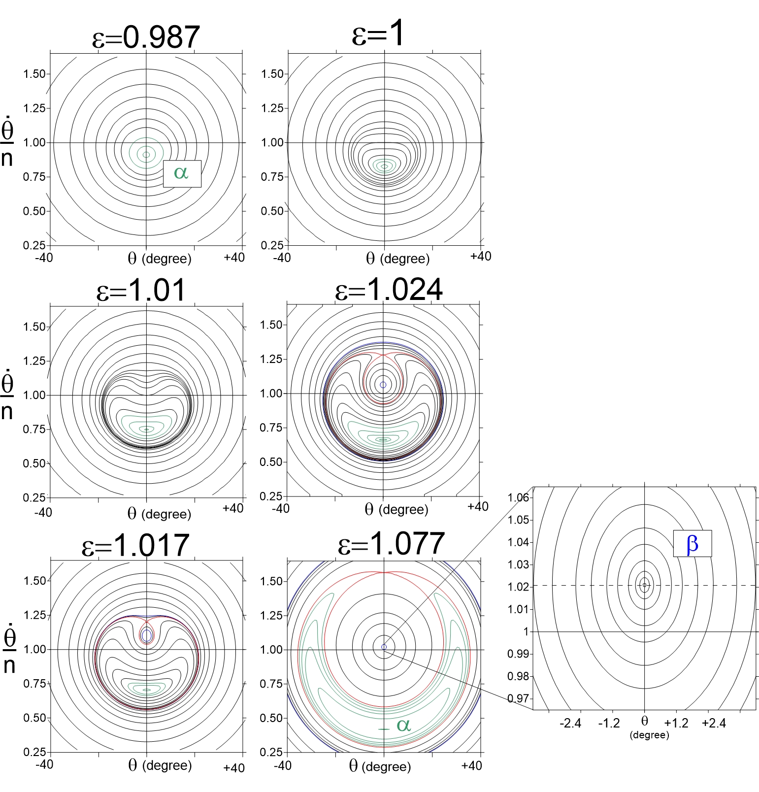
Figure 2: Contour plots of the hamiltonian (26) for several values of the non-sphericity parameter $\epsilon$. The orbital eccentricity is $0.0014$ and the range of values of $\epsilon$ are compatible with the values of Methone ($\epsilon\sim 1.077$ (the same utilized in Fig. 1). Green and blue lines correspond to level curves within the domains of the $\alpha$ and $\beta$-regimes, respectively. Red curves are the separatrix of the $\beta$-regime. Right-bottom plot is a detailed close of the fixed point associated with the $\beta$-regime. The dashed line indicates the forced component.

3.4 The forcing of the $\beta$-regime and the quasi-synchronous regime.

The loci of the equilibria centers (fixed points) of the $\alpha$ and $\beta$-regimes in the phase space can be obtained analytically from equations of motion:

$$\frac{dx}{dt} = +\frac{\partial H}{\partial y}=-\frac{1}{4}(x^{2}+y^{2})y+\delta y+2\gamma_{1}yx$$ (29)

$$\frac{dy}{dt} = -\frac{\partial H}{\partial x}=+\frac{1}{4}(x^{2}+y^{2})x-\delta x-3\gamma_{1}x^{2}-\gamma_{1}y^{2}+\gamma_{2},$$ (30)

where $\gamma_{1}=\frac{3}{8}e\sqrt{\epsilon}$, $\gamma_{2}=e\sqrt{\epsilon^{3}}$.

The equilibria conditions $(\frac{dx}{dt},\frac{dy}{dt})=(0,0)$ lead to a system of non-linear algebraic equations, and equilibria solutions in the x-axis where $y=0$ must satisfy the equation:

$$\frac{x^{3}}{4}-3\gamma_{1}x^{2}-\delta x+\gamma_{2}=0.$$ (31)

The three solutions of Equation (31) are only real for values of $\epsilon$ larger than $\epsilon_{c}$. For $\epsilon<\epsilon_{c}$, only one root is real and there is only one fixed point in the phase space, namely, that one related to the $\alpha$-regime. At $\epsilon=\epsilon_{c}$ occurs the rising of the $\beta$-regime and the unstable point. Considering the current $\epsilon=1.077$ of Methone, the solution of Equation (31) is $(x_{1},x_{2},x_{3})=(-0.5616685,0.02034028,0.5478663)$. Substituting these roots into Equation (28) we obtain $\frac{\dot{\theta}}{n}=0.4171$ ($x_{1}$: $\alpha$-regime); $\frac{\dot{\theta}}{n}=1.0211$ ($x_{2}$: $\beta$-regime); and $\frac{\dot{\theta}}{n}=1.5686$ ($x_{3}$: separatrix). The three values agree with those obtained after inspection of the level curves given Fig. 2. Fig. 3 shows the real solutions calculated in this way in the range of $0.96<\epsilon<1.08$. We can see that the bifurcation occurs at $\epsilon_{c}\sim 1.0149$. Note also the quasi-symmetry of the roots $x_{1}$ and $x_{3}$.

The fixed point of the $\beta$-regime is not centered at the origin as it is indicated by the dashed line in Fig. (2), bottom-right. The forced component calculated above deviates from the unit such that $\frac{\dot{\theta}}{n}=1.0211$. More generally note that in the case of non-circular orbits, $x=0$ is never a solution of Equation (31), so that from Equation (28) the forcing is never null in this case (recall the definition of $\gamma_{1}$).

The forced component in the SOS can also be explained by the classical linear theory of the average solution of the spin-orbit dynamics within the synchronous resonance. The forced harmonic oscillator-analogue model gives $\frac{\dot{\theta}}{n}=1+A$ where the amplitude of the forced component $A$ is given by:

$$A=\frac{2\omega^{2}e}{\omega^{2}-n^{2}}=\frac{2e}{1-\epsilon^{-2}},$$ (32)

(Callegari and Rodríguez 2013; see also equation 5.123 in Murray and Dermott 1999). From Equation (32) we obtain $\frac{\dot{\theta}}{n}=1.0203$, showing good agreement with the value obtained above.

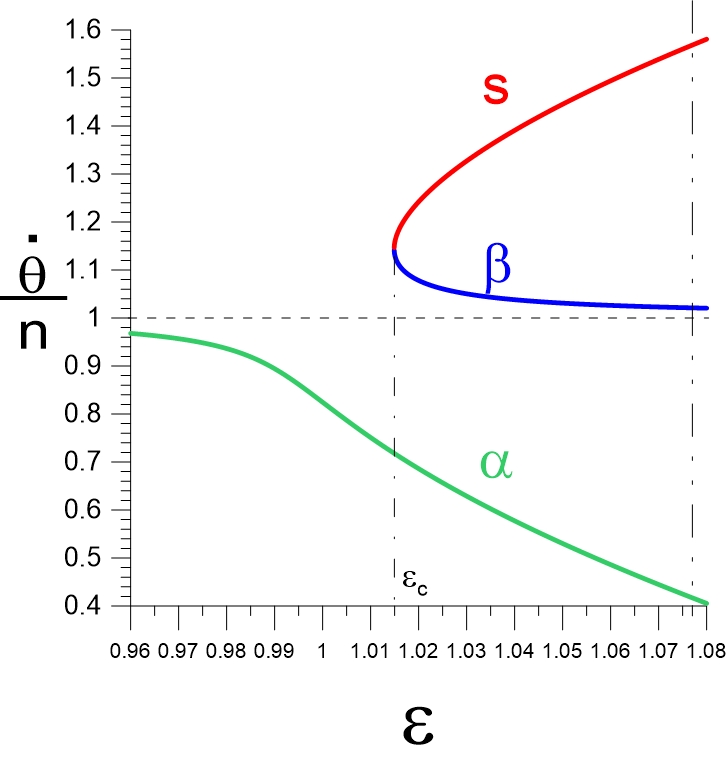
Figure 3: The real roots of Equation (31) as function of $\epsilon$. Red, blue and green curves are the loci of the fixed points of the separatrix ($s$), the $\beta$, and the $\alpha$-regimes, respectively. Dashed horizontal line, dashed-dot-vertical line, and dashed-dot-dot vertical line indicate the straight $\frac{\dot{\theta}}{n}=1$, the critical value $\epsilon_{c}=1.0149$ where the $\beta$-regime rises, and the current value for Methone ($\epsilon=1.077$), respectively.

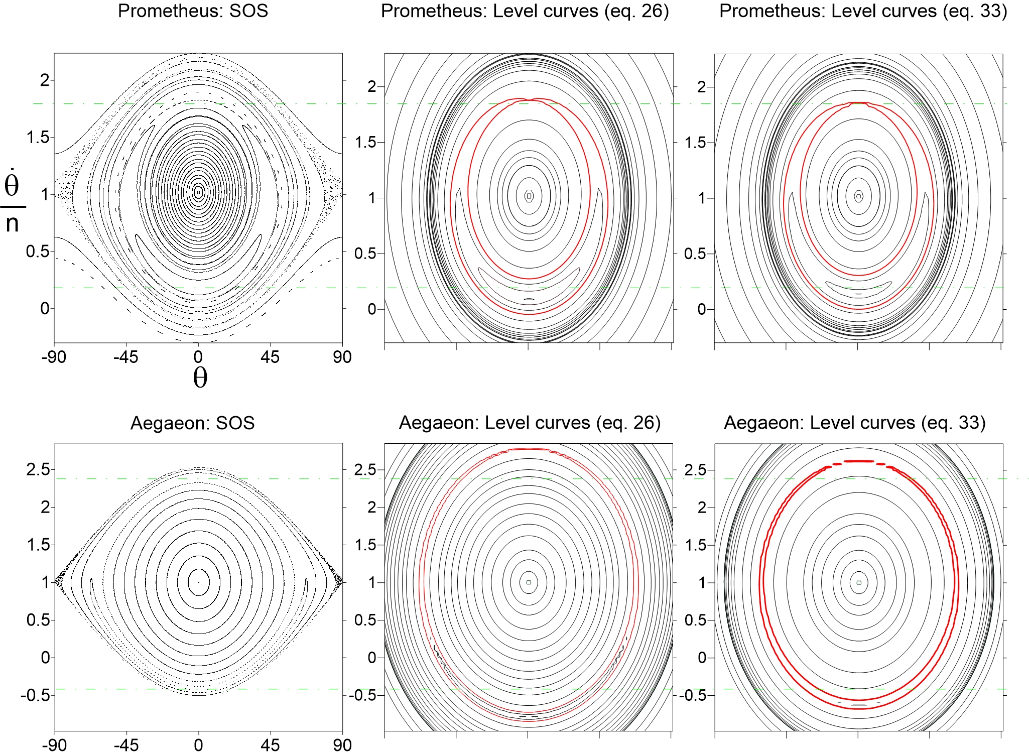
Figure 4: The surfaces of section (SOS; first column), and level curves of the hamiltonian (29) (second column), and (33) (third column) in the cases of Aegaeon and Prometheus (top and bottom, respectively). The separatrix of the $\alpha$-regime is shown in red. Dashed-dot-horizontal lines indicate the fixed points obtained from hamiltonians and compared to the SOS corresponding values.

4 Additional application: Aegaeon and Prometheus.

Fig. (4) shows the rotational phase space around the synchronous regime in the cases of Aegaeon ($\epsilon\sim 1.5236$), and Prometheus ($\epsilon\sim 1.1727$). As pointed out in Section 1, both rotational phase spaces display the $\alpha$ and $\beta$-regimes. Inspection of the left and middle panels shows us that the position of the three fixed points of the $\alpha$ and $\beta$-regimes obtained from level curves (middle) agree with surfaces of section in the case of Prometheus, but the same is not true in the case of Aegaeon.

To improve the model we include terms of order higher than $J^{2}$ in the actions so that the hamiltonian (26) becomes:

$$H(x,y)=\frac{\delta}{2}(x^{2}+y^{2})-\frac{1}{16}(x^{2}+y^{2})^{2}+\frac{3}{8}e\sqrt{\epsilon}(x^{2}+y^{2})x-e\sqrt{\epsilon^{3}}x$$

$$-\frac{1}{128\epsilon}(x^{2}+y^{2})^{3}+\frac{17}{96\sqrt{\epsilon}}e(x^{2}+y^{2})^{5/2},$$ (33)

where terms up to $J^{3}$ have been included (corresponding to the last two terms in Equation (33). A significant improvement can be seen, mainly in the case of Aaegeon. As discussed in Lei (2023), and first shown in Gkolias et al. (2019), in the specific case of the 1:1 secondary resonance, the analytical and numerical mapping of the associated fixed points diverge for values of $\epsilon>1.2$.

5 Conclusions

This work shows the results of the dynamics of rotation of out-of-round close-in small Saturnian satellite Methone and Aegaeon discovered by the Cassini spacecraft. Their shapes and physical parameters have been updated recently by Thomas and Helfenstein (2020). As pointed out in Section 1, the main problem we are considering in this work is related to the nature of the $\alpha$ and $\beta$-regimes of motion in the phase space of rotation of these satellites already detected for Amalthea, Metis, and Prometheus (and probably others - see Melnikov and Shevchenko 2022, and references therein).

We first conduct our investigation with the well-known model of rotation developed by Goldreich and Peale (1966) and applied by many authors in distinct sorts of problems through decades (e.g. Wisdom et al. 1984, Wisdom 2004, Callegari and Rodriguez 2013). The exact equations of the 1.5 degree-of-freedom model are solved numerically Everhart (1985) code, given very accurate rotational trajectories able to identify the main properties of the phase space with the surface of section technique. The $\beta$-regime is located close to the origin and corresponds to the “classical” fixed point associated with the synchronous rotation motion where the amplitude of oscillation of the physical angle $\Psi=\theta-f$ is null at the equilibrium. In the case of Methone, its center is slightly forced by an amount $\sim 0.02$ such that $\frac{\dot{\theta}}{n}\sim 1.02$, a value which can be confirmed by linear theory (Wisdom et al. 1984; Callegari and Rodriguez 2013). The $\alpha$-regime engulfs the $\beta$-regime and it is located far from origin at $\frac{\dot{\theta}}{n}\sim 0.45$ such that $\frac{\dot{\theta}}{n}$ oscillates around 1. Also interestingly the amplitude of variation of $\Psi$ is not null in the equilibrium point of the $\alpha$-regime keeping an amplitude of the order of 30 degrees.

To understand the complexity of such rotation phase space of Methone and Aegaeon, we apply the model developed by Wisdom (2004) to study the rotation of Enceladus. Thus, we follow exactly his steps and reproduce his results; having completed this task, we could apply the methodology to our case. Our hamiltonian (18) generalizes Wisdom’s theory showing all terms at that order of expansion (second order in action). Hamiltonian (33) includes also terms up to $J^{3}$ in the actions. The terms in the expansion involving those which are proportional to 1:1 resonance between the frequency of physical libration $\Psi$ and the mean motion $n$ are responsible for the co-existence of the $\alpha$ and $\beta$ regimes in the rotation of the current Methone and Aegaeon’s phase spaces. Therefore, we have shown the existence of a secondary resonance within the synchronism, completing our initial goals.

Figures (2) and (3) show the dependence of the domains of the $\alpha$ and $\beta$ regimes with the shape parameter of the Methone. The $\beta$-regime occurs at $\epsilon=\epsilon_{c}\sim 1.0149$ such that for $\epsilon<\epsilon_{c}$ only the $\alpha$-regimes exists. While there is good agreement between numerical and analytical calculations in the case of Methone, the same is not true for Aegaeon, where the model is useful only when higher order terms are included in the hamiltonian since $\epsilon>1.2$, a superior limit for convergence of analytical estimative (Gkolias et al. 2019).

We revisit the previous works on the rotation of Prometheus, Amalthea, and Metis given the current theory. The case of Metis is similar to that Methone since $\epsilon\sim 1.0742$ (see Table 1). The case of Amalthea is similar to that of Prometheus since $\epsilon\sim 1.214$ (see Table 1).

As we pointed out above, trajectories within this regime of motion are forced and suffer “long-term” oscillations even in the case of initial conditions located over the fixed point. Being that the current rotational states of Saturnian close-in small satellites are probably synchronous (Thomas and Helfenstein 2020), our results can be taken into account in evolutionary studies of the rotation of these bodies. Tidal models (e.g. Ferraz-Mello et al. 2008, Ferraz-Mello 2013) can be applied to estimate the final destiny of the rotation of such small bodies and also the role of the secondary resonances on its thermal emission (Wisdom 2004).

ACKNOWLEDGEMENTS.

The São Paulo Research Foundation (FAPESP) (process 2020/06807-7).

Prof. Adrián Rodríguez (Valongo Observatory, UFRJ/Brazil).

Part of this work has been presented at the ‘XXI Brazilian Colloquium on Orbital Dynamics’ (INPE, from December 12 to 16, 2022); and at the ‘New Frontiers of Celestial Mechanics: theory and applications’ (Department of Mathematics Tullio Levi-Civita, University of Padua, from February 15 to 17, 2023).

References

- [1] Callegari Jr., N., Rodríguez, A.. Dynamics of rotation of super-Earths. Celest Mech. Dyn. Astr. 116, 389–416 (2013).
- [2] Callegari Jr., N., Ribeiro, F. B.. Computational and Applied Mathematics 34, 423-435 (2015).
-
[3]
Callegari Jr., N., Rodríguez, A., Ceccatto, D. T.. The current orbit of Methone (S/2004 S 1).
Celest. Mech. Dyn. Astr. 133:49 (2021).
-
[4]
Callegari Jr., N., Rodríguez, A..The orbit of Aegaeon and the 7:6 Mimas-Aegaeon resonance.
Celest. Mech. Dyn. Astr. 135:21 (2023).
- [5] Ceccatto, D. T.; Callegari, N., Jr.; Rodríguez, Adrián (2021). The current orbit of Atlas (SXV). Proceedings of the International Astronomical Union, IAU Symposium, 15, 120 - 127.
- [6] Dermott, S. F., Thomas, P. C.. The Determination of the Mass and Mean Density of Enceladus from its Observed Shape. Icarus 109, 241- (1994).
- [7] Everhart, E.. An efficient integrator that uses Gauss-Radau spacings. In: IAU Coloquium 83, 185-202 (1985).
- [8] Ferraz-Mello, S.. Canonical Perturbation Theories - Degenerate Systems and Resonance. Series: Astrophysics and Space Science Library, Vol. 345. Springer US (2007).
- [9] Ferraz-Mello, S., Rodríguez, A., Hussmann, H.. Tidal friction in close-in satellites and exoplanets: The Darwin theory re-visited. Celest. Mech. Dyn. Astr. 101, 171-201 (2008).
- [10] Ferraz-Mello, S.. Tidal synchronization of close-in satellites and exoplanets. A rheophysical approach. Celest. Mech. Dyn. Astr. 116, 109-140 (2013).
- [11] Gkolias, I., Celletti, A., Efthymiopoulos, C., Pucacco, G.. The theory of secondary resonances in the spin–orbit problem. MNRAS, 459, 1327 (2016).
- [12] Gkolias, I., Efthymiopoulos, C., Celletti, A., Pucacco, G.. Accurate Modelling of the low-order resonances in the spin-orbit problem. Communications in Nonlinear Science and Numerical Simulation, 77, 181 (2019).
- [13] Goldreich, P., Peale, S.. Spin-orbit coupling in the solar system. The Astronomical Journal, 71, 425-437 (1966).
- [14] Lei, H.. Dynamical structures associated with high-order and secondary resonances in the spin-orbit problem. https://arxiv.org/pdf/2312.14413.pdf (2023).
- [15] Melnikov, A. V., Shevchenko. On the rotational dynamics of Prometeus and Pandora. Celest Mech. Dyn. Astr. 101, 31-47 (2008).
- [16] Melnikov, A. V., Shevchenko. Rotational Dynamics and Evolution of Planetary Satellites in the Solar and Exoplanetary Systems. Solar System Research, 56, No. 1, pp. 1–22 (2022).
- [17] Murray, C. D, Dermott, S. F.. Solar System Dynamics, Cambridge University Press (1999).
- [18] Pashkevich, V. V. ; Vershkov, A. N. ; Mel’nikov, A. V.. Rotational Dynamics of the Inner Satellites of Jupiter. Solar System Research, 55, Issue 1, p.47-60 (2021).
- [19] Peale, S. J.. Rotation Histories of the Natural Satellites. In: Planetary Satellites. Proceedings of IAU Colloq. 28, held in Ithaca, NY, August 1974. Edited by J. A. Burns. University of Arizona Press, 1977, p.87.
- [20] Porco, C. C.. S/2004 S 1 and S/2004 S 2. IAU Circ. 8401 (2004 August 16) (2004).
- [21] Porco, C. C. S/2008 S 1. IAU Circ. 9023 (2009 March 3) (2009).
- [22] Press, W. H., Teukolsky, S. A., Vetterling, W. T., B. P. Flannery: ‘Numerical Recipes in Fortran 77’. Cambridge University Press (1996).
- [23] Sussman, G. J., Wisdom, J. with Mayer, M. E.: Structure and Interpretation of Classical Mechanics. The MIT Press. Cambridge, Massachusetts (2001).
- [24] Thomas, P.C., J.A. Burns, L. Rossier, D. Simonelli, J. Veverka, C.R. Chapman, K. Klaasen, T.V. Johnson, M.J.S. Belton, Galileo Solid State Imaging Team. The Small Inner Satellites of Jupiter. Icarus, 135, 360-371 (1998).
- [25] Thomas, P. C.; Helfenstein, P.. The small inner satellites of Saturn: Shapes, structures ans some implications. Icarus, 344, 113355 (2020).
- [26] Wisdom, J., Peale, S. J., Mignard, F.. The chaotic rotation of Hyperion. Icarus, 58, 137-152 (1984).
- [27] Wisdom, J.. Spin-Orbit Secondary Resonance Dynamics of Enceladus. The Astronomical Journal 128, 484-491 (2004).