Quantum-Hybrid Stereo Matching
With Nonlinear Regularization and Spatial Pyramids

Abstract

Quantum visual computing is advancing rapidly. This paper presents a new formulation for stereo matching with nonlinear regularizers and spatial pyramids on quantum annealers as a maximum a posteriori inference problem that minimizes the energy of a Markov Random Field. Our approach is hybrid (i.e., quantum-classical) and is compatible with modern D-Wave quantum annealers, i.e., it includes a quadratic unconstrained binary optimization (QUBO) objective. Previous quantum annealing techniques for stereo matching are limited to using linear regularizers, and thus, they do not exploit the fundamental advantages of the quantum computing paradigm in solving combinatorial optimization problems. In contrast, our method utilizes the full potential of quantum annealing for stereo matching, as nonlinear regularizers create optimization problems which are $\mathcal{NP}$-hard. On the Middlebury benchmark, we achieve an improved root mean squared accuracy over the previous state of the art in quantum stereo matching of 2% and 22.5% when using different solvers.

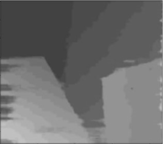
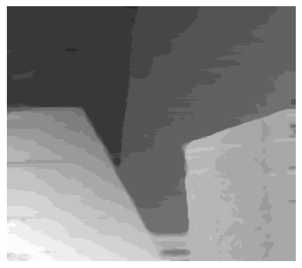
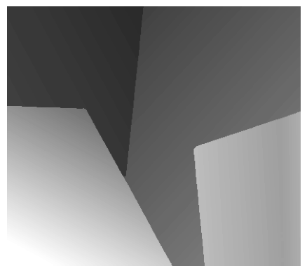
Prior Work	Ours	Ground Truth
$\textit{RMSE}=1.4$	$\textit{RMSE}=0.96$
$\textit{BPP}=9.8$	$\textit{BPP}=8.16$

Figure 1: Stereo estimates on the Middlebury [47] Venus stereo image pair. From left to right: Heidari et al.’s approach [26], our approach and ground truth. In this example, we achieve a $46\%$ decrease in root mean squared error (RMSE) from Heidari et al. and a $10\%$ decrease in bad pixel percentage (BPP). We avoid many of the streaking artifacts present in the result of the prior approach.

1 Introduction

Stereo matching has already been studied for more than a century [25, 19, 36]. It is well understood, and many algorithms exist [32, 30, 52, 27], including recent works leveraging quantum hardware [12, 26]. Despite the fact that quantum computers still cannot compete with classical machines in absolute terms (e.g., absolute execution speed or admissible problem sizes), they promise to provide accelerated solutions in certain cases, including combinatorial optimization problems in the near future. Quantum computing and quantum computer vision are quickly developing and gaining momentum [38, 8, 35]. Hence, the community is investigating how such fundamental computer vision problems as stereo matching could benefit from quantum hardware.

The current leading method for quantum stereo matching from Heidari et al. [26] is based on solving the min-flow-max-cut problem on a quantum annealer. In particular, quantum annealers are theorized to provide advantages in solving Quadratic Unconstrained Binary Optimization (QUBO) problems and, e.g., outperform simulated annealing [29] for certain (rugged) energy landscapes, in terms of the absolute convergence speed and the energy level of the final returned solution [1, 59]. While Heidari et al. [26] achieve useful results, their method is limited to linear regularizers. Moreover, the solution of their approach can be computed in polynomial time and does not leverage the true advantages of quantum computers. Furthermore, it cannot process a complete epipolar line at a time on modern quantum hardware, and has no ability to process data with a large number of disparity labels via coarse-to-fine techniques.

To address these shortcomings, we propose a novel stereo matching formulation for quantum annealers based on Markov Random Fields (MRFs). It allows modeling nonlinear regularizers that lead to $\mathcal{NP}$-hard problems and therefore exploits the true advantages of the quantum computing paradigm. In addition, it allows leveraging a coarse-to-fine pyramid for robust processing, see Fig. 1. A direct comparison to Heidari et al. [26] is challenging, as they use the D-Wave proprietary hybrid solver, and it is unknown to what degree their solution was obtained with traditional solvers or quantum hardware. When reimplementing their method and solving the max-flow-min-cut problem using Ford Fulkerson [20], and comparing it to our method solved with the non-quantum solver Gurobi (i.e., with a non-quantum branch-and-bound optimization), we achieve an RMSE improvement of $2\%$ on average. When directly comparing our Gurobi results to the results of their paper, the improvement is $22.5\%$. Thus, our method overall yields an improvement between $2\%$ and $22.5\%$.

Even though solving the proposed objective on quantum hardware with D-Wave does not result in improved solutions yet due to imperfections of quantum hardware, the proposal of a method with nonlinear regularizers mappable to quantum hardware is a step forward. In summary, our contributions are as follows:

• We present a novel quantum-hybrid approach to stereo matching with MRF energy minimization that is compatible with modern and upcoming quantum hardware.

• For the first time, we show how nonlinear regularizers can be modeled for stereo matching on quantum annealers and the advantages of quantum computers on $\mathcal{NP}$-hard problems can effectively be leveraged.

• We demonstrate that our approach allows integrating a coarse-to-fine pyramid that adds additional regularization and makes the computation tractable with current solvers.

The source code of our approach is available, see our project website for details. The general MRF formulation for quantum annealer optimization can also be applied to other fundamental computer vision tasks, such as optical flow estimation or motion segmentation.

2 Related Work

2.1 Traditional Methods for Stereo Matching

Stereo matching is a fundamental task with a long history. Most recent research focuses on using deep learning to integrate prior knowledge from a training dataset [39, 34]. While these approaches need heavy computing power and perform very well on some datasets, they suffer from robustness and limited generalizability [58, 51]. In contrast, our method is explicit, does not need training data, and uses a quantum computer instead of graphics processing units.

For traditional approaches, Scharstein et al. [47] presented a taxonomy where they introduced the building blocks (1) matching cost computation, (2) cost (support) aggregation, (3) disparity optimization, and (4) disparity refinement. The focus of our work is on (3) as we present a novel way to implement the optimization with a QUBO. For the other building blocks, we follow the baseline [26]. When seeing stereo matching as an optimization problem, it is most common to establish a global energy formulation with a data and smoothness term. In the case of linear regularizers, max-flow-min-cut [46] methods were shown to be efficient and are also the choice of the previous work for quantum annealers [26].

However, when considering the general case and moving to the more robust nonlinear regularizers, the problem becomes $\mathcal{NP}$-hard and many heuristics and algorithms to find a good local minimum have been proposed, including continuation [5], simulated annealing [37, 3], highest confidence first [11] and mean-field annealing [23]. The most popular traditional techniques that allow leveraging nonlinear regularizers and stand in contrast to ours are belief propagation [53] and semi-global matching [27]. However, these require iterative updates and cannot be formulated as a QUBO. Unlike prior work in this area, we use quantum annealers to tackle an $\mathcal{NP}$-hard problem.

2.2 Quantum Computer Vision

Quantum Computer Vision (QCV) is an emerging field and many methods for different problems were proposed over the last years, such as object tracking [60], robust fitting [15] and motion segmentation [2]. Several techniques tackle correspondence problems across two or more instances, i.e., graph and matching [49], mesh alignment [50], point set registration [40, 43] and stereo matching [12, 26].

The method of Heidari et al. [26] leverages the graph cut formulation introduced by Cruz-Santos et al. [12], and is the closest work to ours, but in contrast, does not allow for nonlinear regularizers and is solvable in linear time. The quantum stereo matching method of Heidari et al. [26] is the closest work to ours. It casts stereo matching as a min-flow max-cut problem converted into a QUBO problem using techniques introduced by Cruz-Santos et al. [12], which were improved upon by Krauss et al. [33]. Alternatively, stereo matching can be formulated as an MRF MAP (Markov Random Field Max a Posteriori) inference, and we follow this approach. To this end, we show how an MRF MAP inference can be transformed into a QUBO. Our QUBO requires the same number of binary variables as Heidari et al. when considering the same region and number of disparities. Although the topological complexity of our QUBO will grow faster than in [26] as the number of possible disparities increases, it will still remain relatively sparse. The use of a coarse-to-fine pyramid allows us to fully embed practical problems onto modern quantum hardware, which was not possible in [26].

Our method stands in contrast to Presles et al. [45], which solves an MRF MAP via a graph cut. They introduce an ancillary variable $z_{\alpha}$ which must connect to all original variables. Since $z_{\alpha}$ will have so many connections, embedding this QUBO problem onto a quantum annealer will be difficult, and this difficultly will scale poorly as the problem grows. Additionally, to enforce that their connected ancillary variable $z_{\alpha}$ is always $1$, they must set the corresponding weight to be extremely negative. This can cause the annealer’s energy landscape to be extremely jagged and lead to lower accuracy. Another method for formulating MRF MAP inferences as QUBOs [44] is limited to the binary MRF case, which severely limits the scope of the practical problems which their formulation can solve. In contrast, ours is applicable to any label space size.

3 Method

3.1 Background

We aim at a formulation compatible with experimental adiabatic quantum annealers such as D-Wave. Unlike gate-based quantum computers, the adiabatic quantum annealers are already suitable for practically relevant combinatorial optimization problems, and provide a speed-up over traditional machines in solving them [1, 59]. D-Wave exclusively supports Quadratic Unconstrained Binary Optimization (QUBO) objectives and, hence, all target tasks, including possible boundary conditions, must be converted to a QUBO before quantum annealing can be attempted.

Let $\mathbf{x}\in\{0,1\}^{n}$ be a binary vector of length $n$. A QUBO problem is defined as finding $\mathbf{x}^{*}$ such that:

$$\mathbf{x}^{*}=\text{argmin}_{\mathbf{x}\in\{0,1\}^{n}}\mathbf{x}^{T}Q\mathbf{x}\,\,,$$ (1)

where $Q\in\mathbb{R}^{n\times n}$ is symmetric. $\mathbf{x}^{T}Q\mathbf{x}$ is the quadratic form of $Q$, i.e., it is a polynomial in terms of the entries of $\mathbf{x}$ of at most degree $2$.

Quantum annealers solve (1) by mapping the QUBO onto a quantum-mechanical system consisting of qubits. A qubit is an object small enough to have its behavior be governed by quantum mechanics. When we measure a qubit, we will observe it to be either the state $\ket{0}$ or $\ket{1}$. The possible energies of the annealer’s system are described by a quantum mechanical operator called the Hamiltonian, $\mathcal{H}_{P}$. By measuring the state of every qubit in the system, and by referring to $\mathcal{H}_{P}$, we can determine the total energy of the system. In our mapping, each binary variable in $\mathbf{x}$ is mapped to a qubit, and $Q$ is mapped to $\mathcal{H}_{P}$ such that when the qubits are measured, the system’s total energy is equal to $\mathbf{x}^{T}Q\mathbf{x}$. We seek to measure the ground (i.e., lowest-energy) state of the system as permitted by $\mathcal{H}_{P}$, as this is equivalent to finding $\mathbf{x}^{*}$. Even if we cannot measure the ground state, any low energy state should be a reasonably close solution to the QUBO.

In these terms, quantum annealing (QA) works as follows: The annealer initializes with possible energies described by a standard initial Hamiltonian $\mathcal{H}_{I}$, and with qubits in the known ground state. Next, during annealing, the system smoothly transitions from being described by $\mathcal{H}_{I}$ to $\mathcal{H}_{P}$. The adiabatic theorem of quantum mechanics [7] states that if the interpolation between $\mathcal{H}_{I}$ and $\mathcal{H}_{P}$ is slow enough, the system will have a non-zero (and often high) probability to remain in its ground state. After annealing, the state of the system is measured. Ideally, this is the ground state of $\mathcal{H}_{P}$, however it might only be close to the ground state. Annealing is often run many times, with the measured state with the minimal energy being returned as the proposed QUBO solution.

Further details on qubit measurement and the speed ranges of $\mathcal{H}_{I}$ to $\mathcal{H}_{P}$ transitions can be found in Nielsen and Chuang [42] and the works by Farhi et al. [17, 18]. However, for the remainder of this paper, it is only important to understand that our problem needs to be formulated as a QUBO (1).

3.2 Formulating MRF MAP as a QUBO

Following the notation in Drory et al. [16], a Markov Random Field (MRF) can be formulated as an undirected graph $\mathcal{G}=(\mathcal{V},\mathcal{E})$, where each vertex $\mathbf{v}\in\mathcal{V}$ has a label $\ell_{\mathbf{v}}$ from a discrete set $\mathcal{L}_{\mathbf{v}}$, and there are unary costs $\varphi_{\mathbf{v}}(\ell_{\mathbf{v}})$ and binary costs $\varphi_{\mathbf{p},\mathbf{q}}(\ell_{\mathbf{p}},\ell_{\mathbf{q}})$ for $(\mathbf{p},\mathbf{q})\in\mathcal{E}$. The energy of the MRF is then defined as:

$$E(\ell_{(\cdot)})=\sum_{\mathbf{v}\in\mathcal{V}}\varphi_{\mathbf{v}}(\ell_{\mathbf{v}})+\sum_{(\mathbf{p},\mathbf{q})\in\mathcal{E}}\varphi_{\mathbf{p},\mathbf{q}}(\ell_{\mathbf{p}},\ell_{\mathbf{q}})\,\,.$$ (2)

Finding the labelling $\ell_{(\cdot)}$ such that $E(\ell_{(\cdot)})$ is minimal is the MRF maximum a posteriori (MAP) inference problem, which is $\mathcal{NP}$-hard in general [31, pg.551]. This motivates us to use adiabatic quantum computing and in this subsection, we will show how such a general MRF can be mapped to a QUBO. Subsequently, we will show how stereo matching can be formulated as an instance of an MRF and solved in a quantum-hybrid manner. Notably, the QUBO formulation of an MRF is general and could be applied to a wide range of other problems in the future.

A binary encoding scheme for our Markov variable labels (to be encoded into a QUBO) is conceivable (see Appendix B); this approach would avoid introducing rectifiers necessary with our other scheme and, therefore, may increase the annealing stability. Unfortunately, the number of QUBO binary variables required to represent the MRF in this case grows exponentially with the number of labels, which quickly becomes infeasible with current and likely near-term future hardware. For a full analysis on embedding complexities of all schemes, see Appendix C.

Therefore, we proceed with a one-hot encoding scheme of the Markov variable labels together with a novel local rectifier that minimizes the disturbances during annealing. For a given vertex $\mathbf{v}$, the set of labels is denoted by $\mathcal{L}_{\mathbf{v}}$ and is enumerated by the index $l$. For each possible label value $\ell_{\mathbf{v}}^{l}$, we create a corresponding binary variable $\mathbf{x}_{\ell_{{}_{\textbf{v}}}^{l}}$:

$$\mathbf{x}_{\ell_{\mathbf{v}}^{l}}=\begin{cases}1&\text{if }\ell_{\mathbf{v}}=\ell_{\mathbf{v}}^{l}\,\,,\\ 0&\text{else\,\,.}\end{cases}$$ (3)

This allows us to rewrite Eq. 2 as:

$$\begin{split}E(\ell_{(\cdot)})&=\sum_{\mathbf{v}\in\mathcal{V}}\,\sum_{\ell_{\mathbf{v}}^{l}\in\mathcal{L}_{\mathbf{v}}}\varphi_{\mathbf{v}}(\ell_{\mathbf{v}}^{l})\mathbf{x}_{\ell_{\mathbf{v}}^{l}}^{2}+\\ &+\sum_{(\mathbf{p},\mathbf{q})\in\mathcal{E}}\,\sum_{\ell_{\mathbf{p}}^{r}\in\mathcal{L}_{\mathbf{p}}}\,\sum_{\ell_{\mathbf{q}}^{s}\in\mathcal{L}_{\mathbf{q}}}\varphi_{\mathbf{p},\mathbf{q}}(\ell_{\mathbf{p}}^{r},\ell_{\mathbf{q}}^{s})\mathbf{x}_{\ell_{\mathbf{p}}^{r}}\mathbf{x}_{\ell_{\mathbf{q}}^{s}}\,\,.\end{split}$$ (4)

Next, we can write our Markov random field cost as a quadratic polynomial in terms of a collection of binary variables. To bring the cost from Eq. 4 into the quadratic form (1), we define the binary vector $\mathbf{x}$ as

$$\mathbf{x}=\{\mathbf{x}_{\ell_{\mathbf{v}}^{l}}\}_{\forall\mathbf{v}\in\mathcal{V},\,\forall\ell_{\mathbf{v}}^{l}\in\mathcal{L}_{\mathbf{v}}}\,\,.$$ (5)

We index entries of $Q$ by $\ell_{\mathbf{p}}^{r},\ell_{\mathbf{q}}^{s}$ and define them as follows:

$$\small\begin{split}\forall\mathbf{v}\in\mathcal{V},\,\forall\ell_{\mathbf{v}}^{l}\in\mathcal{L}_{\mathbf{v}}:\,\,Q_{\ell_{\mathbf{v}}^{l},\ell_{\mathbf{v}}^{l}}&=\varphi_{\mathbf{v}}(\ell_{\mathbf{v}}^{l})\\ \forall(\mathbf{p},\mathbf{q})\in\mathcal{E},\,\forall\ell_{\mathbf{p}}^{r}\in\mathcal{L}_{\mathbf{p}},\,\forall\ell_{\mathbf{q}}^{s}\in\mathcal{L}_{\mathbf{q}}:\,\,Q_{\ell_{\mathbf{p}}^{r},\ell_{\mathbf{q}}^{s}}&=\frac{1}{2}\varphi_{\mathbf{p},\mathbf{q}}(\ell_{\mathbf{p}}^{r},\ell_{\mathbf{q}}^{s})\\ \,\,Q_{\ell_{\mathbf{q}}^{s},\ell_{\mathbf{p}}^{r}}&=\frac{1}{2}\varphi_{\mathbf{q},\mathbf{p}}(\ell_{\mathbf{q}}^{s},\ell_{\mathbf{p}}^{r})\,\,.\end{split}$$ (6)

All other entries of $Q$ are $0$. We have now translated our label from Eq. 4 into the matrix quadratic form:

$$\mathbf{x}^{T}Q\mathbf{x}=E(\ell_{(\cdot)})\,\,.$$ (7)

Note, however, that we cannot submit $Q$ to a quantum annealer in its current form as we must enforce that for every vertex we have only one label assigned, i.e., there must be exactly one binary variable $x_{\ell_{\mathbf{v}}^{l}}$ that is equal to $1$. We can express this constraint as:

$$\forall\mathbf{v}\in\mathcal{V}:\sum_{\forall\ell_{\mathbf{v}}^{l}\in\mathcal{L}_{\mathbf{v}}}\mathbf{x}_{\ell_{\mathbf{p}}^{l}}=1\,\,.$$ (8)

Following the techniques proposed in QSync [4], we can incorporate this constraint by tweaking our definition of $Q$ from Eq. 6 into the following form:

$$\small\begin{split}\forall\mathbf{v}\in\mathcal{V},\,\forall\ell_{\mathbf{v}}^{l}\in\mathcal{L}_{\mathbf{v}}:&\,\,Q_{\ell_{\mathbf{v}}^{l},\ell_{\mathbf{v}}^{l}}=\varphi_{\mathbf{v}}(\ell_{\mathbf{v}}^{l})-\Lambda(\ell_{\mathbf{v}}^{l},\ell_{\mathbf{v}}^{l})\\ \forall\mathbf{v}\in\mathcal{V},\,\forall\ell_{\mathbf{v}}^{r},\ell_{\mathbf{v}}^{s}\in\mathcal{L}_{\mathbf{v}},\,r\neq s:&\,\,Q_{\ell_{\mathbf{v}}^{r},\ell_{\mathbf{v}}^{s}}=\Lambda(\ell_{\mathbf{v}}^{r},\ell_{\mathbf{v}}^{s})\\ &\,\,Q_{\ell_{\mathbf{v}}^{s},\ell_{\mathbf{v}}^{r}}=\Lambda(\ell_{\mathbf{v}}^{r},\ell_{\mathbf{v}}^{s})\\ \forall(\mathbf{p},\mathbf{q})\in E,\forall\ell_{\mathbf{p}}^{r}\in\mathcal{L}_{\mathbf{p}}\forall\ell_{\mathbf{q}}^{s}\in\mathcal{L}_{\mathbf{q}}:&\,\,Q_{\ell_{\mathbf{p}}^{r},\ell_{\mathbf{q}}^{s}}=\frac{1}{2}\varphi_{\mathbf{p},\mathbf{q}}(\ell_{\mathbf{p}}^{r},\ell_{\mathbf{q}}^{s})\\ &\,\,Q_{\ell_{\mathbf{q}}^{s},\ell_{\mathbf{p}}^{r}}=\frac{1}{2}\varphi_{\mathbf{p},\mathbf{q}}(\ell_{\mathbf{p}}^{r},\ell_{\mathbf{q}}^{s}),\\ \end{split}$$ (9)

with the unmentioned entries of $Q$ being $0$. The common rectification scheme is to set $\Lambda(\ell_{\mathbf{v}}^{r},\ell_{\mathbf{v}}^{s})=\lambda_{\mathbf{v}}$, with $\lambda_{\mathbf{v}}$ being a vertex-specific constant which enforces that only one label per vertex should have a coefficient of $1$. However, a higher $\Lambda$ leads to a more jagged energy landscape on the quantum annealer and negatively affects its results. Thus, one would like to set the $\Lambda$ as small as possible (see Appendix F for details). To this end, we derive a function $\Lambda(\cdot,\cdot)$ that yields a sufficiently high upper bound while obeying our constraints. The full derivation of $\Lambda(\cdot,\cdot)$ is presented in Appendix A.

3.3 Stereo Matching as an MRF MAP

Let $\{I^{L},I^{R}\}$ be a set of grayscale stereo images defined over the pixel grid domain $\Omega\subset\mathbb{N}^{2}$. We assume that our images are rectified, meaning that the per-point displacements in the image plane lie on horizontal epipolar lines and are positive. We denote the disparity at image coordinates $(i,j)$ with $d_{i,j}$ and the matrix containing all disparities as $D$. There are many works that treat stereo matching as an energy minimization problem [26, 57, 41], where the energy is the sum of a data term $E_{d}(d_{i,j})$ across $D$ and a smoothness term $E_{s}(d_{i,j},d_{i^{\prime},j^{\prime}})$ with $(i,j)$ and $(i^{\prime},j^{\prime})$ being from the set $\mathcal{N}$ of neighboring pixels. The data term should be lower when the estimated disparities map to similar regions in the second image. In our case, it relies on the brightness constancy assumption [22, 26]:

$$E_{d}(d_{i,j})=(I^{L}(i,j)-I^{R}(i-d_{i,j},j))^{2}\,.$$ (10)

The smoothness term should be lower when the disparities maintain local structural coherence. We use a truncated (nonlinear) regularizer with edge-awareness:

$$E_{s}(d_{i,j},d_{i^{\prime},j^{\prime}})=\begin{cases}R\text{ if }|I^{L}(i,j)-I^{L}(i^{\prime},j^{\prime})|\leq\tau\\ R/q\text{ else }\end{cases},$$ (11)

with

$$R=\operatorname{min}(m,s\,|d_{i,j}-d_{i^{\prime},j^{\prime}}|),$$ (12)

where $\tau$, $q$, $m$ and $s$ are tunable hyperparameters. Similar ideas for nonlinear, edge aware regularizers were discussed in the literature before [48]. This nonlinear regularizer makes the resulting total energy function (See Eq. 13 $\mathcal{NP}$-hard to minimize. At the same time, this regularizer has only a few hyperparameters, making it relatively simple to tune and optimize. Throughout Sec. 4, we fix our regularization parameters across all experiments. The values of all the parameters at each iteration of our coarse-to-fine algorithm are given in Appendix D.

We can now define our total energy functional $E(D)$ as

$$E(D)=\sum_{(i,j)\in\Omega}E_{d}(d_{i,j})+\sum_{((i,j),(i^{\prime}j^{\prime}))\in\mathcal{N}}E_{s}(d_{i,j},d_{i^{\prime},j^{\prime}})\,.$$ (13)

We seek the disparity matrix $D^{*}$ that minimizes $E(D)$. Notably, the transformation into an MRF is straight forward with

$$\small\begin{split}&\mathcal{V}=\Omega\,,\,\mathcal{E}=\mathcal{N}\,,\,\ell_{i,j}=d_{i,j}\,,\varphi_{(i,j)}(\ell_{i,j})=E_{d}(d_{i,j})\,\,\text{and}\,\\ &\varphi_{(i,j),(i^{\prime},j^{\prime})}(\ell_{i,j},\ell_{i^{\prime},j^{\prime}})=E_{s}(d_{i,j},d_{i^{\prime},j^{\prime}})\,.\\ \end{split}$$ (14)

3.4 Our Stereo Matching Algorithm

We now describe our full method for stereo matching that leverages adiabatic quantum computing. When given an image pair, we first precalculate $E_{d}(d_{i,j})$ and $E_{s}(d_{i,j},d_{i^{\prime},j^{\prime}})$ for all considered disparity sizes on a traditional machine. Following the derivation in the previous sections, we then produce the matrix $Q$, which we can submit to either a traditional QUBO solver or a quantum annealer. In either case, we receive the binary vector $\mathbf{x}^{*}$ as a response that we decode into the disparity matrix $D^{*}$.

As the QUBO formulations of stereo estimation problems can become too large to be mapped to quantum hardware or even solved directly with a traditional optimizer, we employ a coarse-to-fine strategy. First, we downsample the images by a factor of $4$ in each dimension, and solve the QUBO for $6$ possible disparities per pixel, corresponding to disparities of $0$, $4$, $8$, $12$, $16$, and $20$ on the full resolution. We then upsample by $2$ to proceed to the next higher resolution, this time considering $4$ possible labels. Finally, we upsample to full resolution and consider $4$ possible labels. This method allows us to consider a sufficient number of disparity levels arising in stereo matching problems. The method can, in theory, be just as accurate with only two coarse-to-fine iterations, one at the downsample factor of $4$, and one at full resolution. However, we found that including intermediate coarseness layers allows for some ability to correct errors and yields the best results (see  Appendix E).

To reduce the QUBO size further, we split the problem into bundles of epipolar lines and solve for each bundle individually. Similar to Heidari et al. [26], we observe that the solutions obtained by our method are still noisy. Therefore, we follow their denoising approach and apply median filtering to our disparity estimate at each resolution before upsampling, and bilateral filtering [56] as a final post-processing step. We have now obtained a quantum-hybrid method for stereo matching that can leverage modern quantum hardware for combinatorial optimization objectives. A full overview of the method is given in Algorithms 1 and 2.

Algorithm 1 Coarse-to-Fine Stereo Matching

1:procedure Stereo Match($I^{L},I^{R}$)

2:    $\textit{resolutions}\leftarrow[\frac{1}{4},\frac{1}{2},1]$

3:    $\textit{disparity ranges}\leftarrow[6,4,4]$

4:    $\mathcal{D}^{*}\leftarrow 0$

5:    for step in $[1,2,3]$ do

6:         $\textit{r}\leftarrow\textit{resolutions}[\texttt{step}]$

7:         $\textit{dr}\leftarrow\textit{disparity ranges}[\texttt{step}]$

8:         $\textit{pd}\leftarrow\textsc{Disparity Ranges At Res}(r,dr,\mathcal{D}^{*})$

9:         $I^{L}_{\texttt{step}}\leftarrow\textsc{Resize}(I^{L},r)$

10:         $I^{R}_{\texttt{step}}\leftarrow\textsc{Resize}(I^{R},r)$

11:         $E_{d}\leftarrow\textsc{Build Data Terms}(pd,I^{L}_{\texttt{step}},I^{R}_{\texttt{step}})$

12:         $E_{s}\leftarrow\textsc{Build Smoothness Terms}(pd,I^{L}_{\texttt{step}},I^{R}_{\texttt{step}})$

13:         $\varphi_{\mathbf{p}}\leftarrow E_{d}$ $\triangleright$ Convert to MRF notation

14:         $\varphi_{\mathbf{p},\mathbf{q}}\leftarrow E_{s}$ $\triangleright$ Convert to MRF notation

15:         $\ell^{*}\leftarrow\textsc{Solve MRF MAP}(\varphi_{\mathbf{p}},\varphi_{\mathbf{p},\mathbf{q}})$ (Algorithm 2)

16:         $\mathcal{D}^{*}\leftarrow\ell^{*}$ $\triangleright$ Convert from MRF notation

17:         $\mathcal{D}^{*}\leftarrow\textsc{Full Size From Resolution}(\mathcal{D}^{*},r)$

18:         $\mathcal{D}^{*}\leftarrow\textsc{Median Filter}(\mathcal{D}^{*})$

19:    end for

20:    $\mathcal{D}^{*}\leftarrow\textsc{Bilateral Filter}(\mathcal{D}^{*})$

21:    return $\mathcal{D}^{*}$

22:end procedure

Algorithm 2 MRF MAP Solver via QUBO

1:procedure Solve MRF MAP($\varphi_{\mathbf{p}},\varphi_{\mathbf{p},\mathbf{q}}$)

2:     $Q\leftarrow\textsc{Encode QUBO}(\varphi_{\mathbf{p}},\varphi_{\mathbf{p},\mathbf{q}})$ (Eq. 9)

3:     $x^{*}\leftarrow\textsc{Anneal}(Q)$ $\triangleright$ D-Wave or trad. solver

4:     $\ell^{*}\leftarrow\textsc{Decode Annealer Response}(x^{*})$

5:     return $\ell^{*}$

6:end procedure

4 Experimental Results

For the following sections, we follow Heidari et al. [26] and test on four stereo matching pairs from the Middlebury 2001 dataset [47]: Tsukuba, Bull, Venus, and Sawtooth. We use the root mean squared error (RMSE) and bad pixel percentage (BPP) [47] with $\delta_{d}:=1$ for numerical evaluations.

4.1 Our Experimental Setting

There are many traditional methods to solve QUBO problems. For non-quantum methods, we selected Gurobi [24] and simulated annealing [29]. Gurobi uses branch and bound optimization to find a solution near the global optimum within a tight margin. Its output can be viewed as what an ideal quantum annealer would produce. Simulated annealing is a traditional global optimization technique to solve non-convex problems and can be seen as a simulation of a thermal annealing process. We use D-Wave’s simulated annealer with default parameters [14].

To test with quantum annealing, we use D-Wave’s Pegasus QPU with ${\sim}5.4\cdot 10^{4}$ qubits [6]. To compute the minor embeddings onto Pegasus, we use D-Wave’s minorminer, which by default relies on Cai et al.’s algorithm [10]. Minor embedding is required as physical qubits have limited connectivity, and the logical (or analytically derived qubits) often need to be mapped to chains of physical qubits to enable sampling of a given problem. A minor embedding is a mapping of QUBO binary variables to specific hardware qubits on the QPU. Since physical qubits are connected in a pre-defined pattern (with limited connectivity), a single binary variable must be often mapped to chains of qubits to represent an arbitrary QUBO correctly. Lastly, we tested our approach on closed-source D-Wave’s hybrid solver, which uses traditional optimization in conjunction with quantum annealing. For all techniques involving quantum annealers or simulated annealing, we allow $500$ annealing runs and take the lowest energy solution. All other settings involving D-Wave’s API are set to the default (i.e., annealing time of $20\mu$sec, a majority voting policy for resolving broken chains of physical qubits, and a chain strength calculated as $C=1.414R\sqrt{D}$, with $R$ being the standard deviation of quadratic QUBO coefficients and $D$ being the average degree of QUBO problem nodes).

	Tsukuba	Bull	Sawtooth	Venus
——LI
—–GT
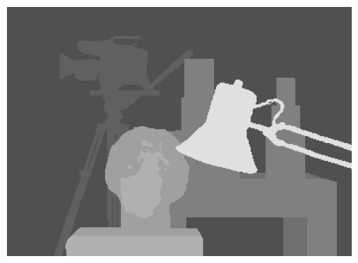
–Ours (G)
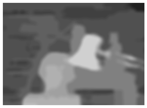
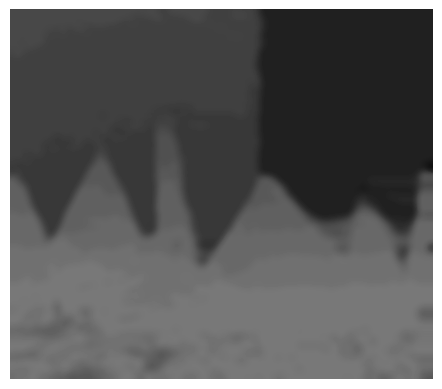
-Ours (SA)
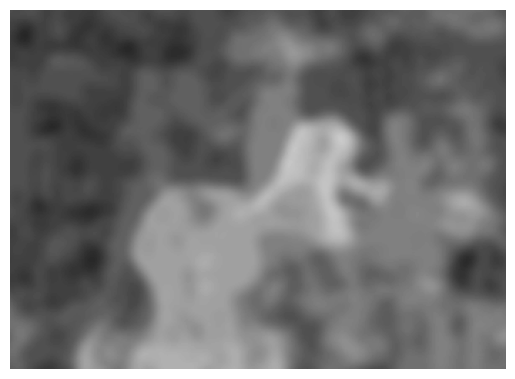
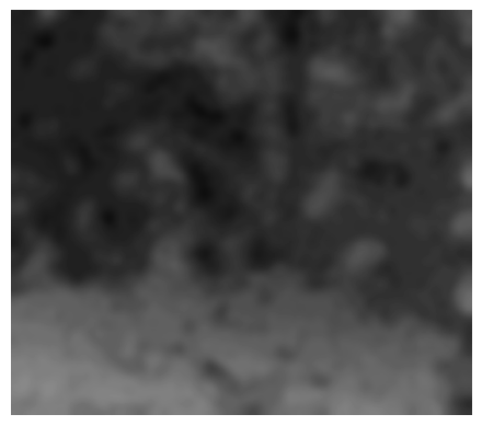
–Ours (H)
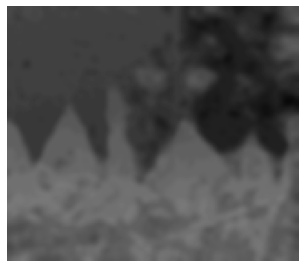
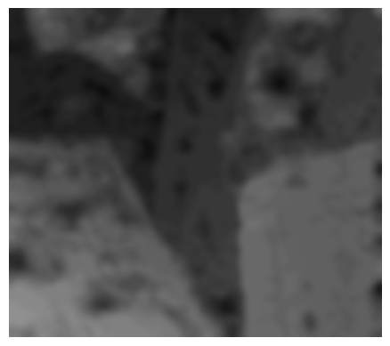
–Ours (Q)

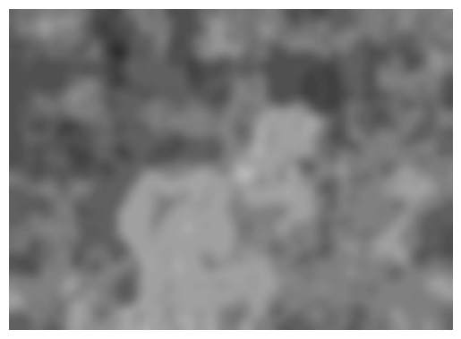
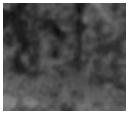
Figure 2: The first row shows the Left Image from each of the four Middlebury stereo pairs. The second row shows the Ground-Truth displacements for each pair. The remaining rows show results by our method using different optimizers: Gurobi, Simulated Annealing, D-Wave’s Hybrid Quantum-Classical Solver, and the D-Wave’s Pegasus QPU. The choice of optimizer has a strong influence on the result quality, and we observe that the traditional optimizer Gurobi outperforms all other methods. We hypothesize that this is because of the jagged and challenging energy landscape for the tested quantum annealer caused by our rectifiers and the current state of quantum hardware.

For the experiments, we restrict our bundles to be a single epipolar line. First, this makes our results more comparable to the previous quantum-admissible stereo matching approach [26] that also operates solely on single epipolar lines. Second, a single epipolar line problem from the Middlebury dataset is sufficiently small to embed onto current D-Wave hardware at all three coarseness levels. We provide a visualization of the different results in Fig. 2 and numerical results in Tab. 1.

Our method performs best when using Gurobi. We conjecture that this is because introducing constraints into a QUBO (i.e., rectification of the QUBO data term) can disrupt the energy landscape and impede the annealing process. For a deeper discussion of this phenomenon, we refer to Birdal and Golyanik et al. [4]. Note that future annealers are expected to improve their properties in sampling of more and more challenging energy landscapes, and achieve performance similar to and even better than Gurobi.

Due to the success of the Gurobi optimizations, for subsequent results, we use it unless stated otherwise. In Fig. 3, we visualize the coarse-to-fine steps of our method. Similar to the previous quantum stereo matching approach [26], the initial results are noisy, while applying median filtering is able to remove the noise effectively. In all the annealing-based methods, we observe splotchy artifacts, which come from coarser resolutions of the pyramid and represent a drawback of coarse-to-fine methods: even with intermediate filtering for corrections, small errors can compound.

In the Gurobi case, these splotchy artifacts are negligible. However, some minor artifacts are still apparent. The streaking patterns (particularly clear on Tsukuba) are likely to occur when one optimizes the epipolar lines independently. We can also see such artifacts in Heidari et al. [26]. The Sawtooth example has two additional unwanted artifacts: over-regularization along the jagged edges, and some general inaccuracies in the lower left region. The over-regularization can be attributed to an incompatible parameterization of our regularizer. We have to select hyperparameters which work well in general, and these jagged edges are a corner case. We conjecture that the poor estimation in the lower left region is also due to our energy model parameterization. The images have a lot of texture in that region of the frame which is misinterpreted as edges of objects, causing under regularization. Additionally, the texture contains repeating brightnesses across the epipolar line, weakening our brightness constancy assumption.

Image Pair Gurobi Simulated Annealing Hybrid QPU RMSE BPP RMSE BPP RMSE BPP RMSE BPP Tsukuba 1.53 12.93 1.87 30.64 1.79 26.82 2.24 45.62 Bull 0.58 3.46 1.86 45.29 1.66 31.57 3.51 76.98 Sawtooth 1.89 24.51 2.27 47.73 2.71 47.49 3.99 74.24 Venus 0.96 8.16 3.04 56.75 2.17 42.43 3.24 67.70 Average 1.24 12.27 2.26 45.10 2.08 37.08 3.25 66.14

Table 1: The Root Mean Squared Error (RMSE) and Bad Pixel Percentage (BPP) of our method using all the optimizers used in Fig. 2. Gurobi outperforms all other optimizers on both metrics

	Pre-Median Filtering	Post-Median Filtering
—–$\frac{1}{4}$  Resolution
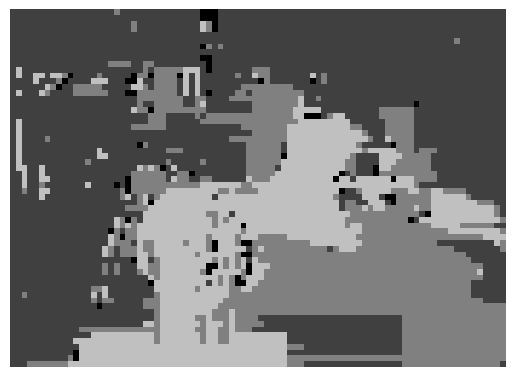
—–$\frac{1}{2}$  Resolution
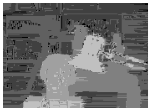
—–Full Resolution

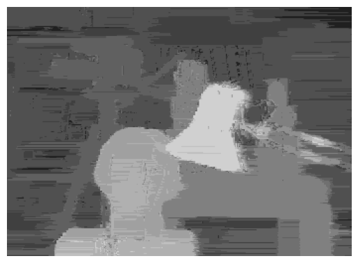
Figure 3: Stereo estimation on the Tsukuba image pair at the three resolution levels, before and after median filtering using the Gurobi solver. Median filtering helps to prevent cascading errors from lower resolution estimates. The final result after bilateral filtering is shown in Fig. 2.

4.2 Comparison to Heidari et al. [26]

We compare our results to those of Heidari et al.’s [26]. However, when making such a comparison, we note that D-Wave’s hybrid optimizer is proprietary. Therefore, it is impossible to diagnose to what degree Heidari et al.’s QUBO problems were optimized with traditional or quantum hardware. To this end, we compare our method using Gurobi against Heidari et al.’s and find that according to Tab. 2 ours is $22.5\%$ better in RMSE on average, although we do have a higher BPP. This can be considered an upper bound of the performance improvement we can achieve. We also considered how Heidari et al.’s results would look if they used classical optimization. For the classical optimization of their formulation, we solved the max-flow min-cut problem using the Ford Fulkerson algorithm [20]. We do not have access to their regularization weight, and determined a value empirically that we found to yield strong performance. Even in this case, our method has a $2\%$ improvement in RMSE over Heidari et al. We conclude that the improvement due to our method lies between $2\%$ and $22.5\%$.

We compare our results visually in Fig. 4 and numerically in Tab. 2. For added context, we also include the result of using D-Wave’s Hybrid optimizer on our method, even though we cannot directly compare to Heidari et al. for the reasons given above. In comparison to Heidari et al.’s hybrid results, our Gurobi results have significantly fewer streaking artifacts. This can be partially explained by the fact that Heidari et al.’s technique only optimizes a single epipolar line at a time. However, because we lack full access to D-Wave’s complete hybrid algorithm, we cannot say for certain. When comparing our Gurobi results to Heidari et al.’s method optimized with Ford Fulkerson [20], we observe that their method has better estimates in the lower left region of Sawtooth than our approach. We suspect this is because Heidari et al.’s method has no coarse-to-fine steps, which are leading to estimation errors for Sawtooth (See Appendix E for a full discussion).

	Tsukuba	Bull	Sawtooth	Venus
Ours (H)
Heidari(H)
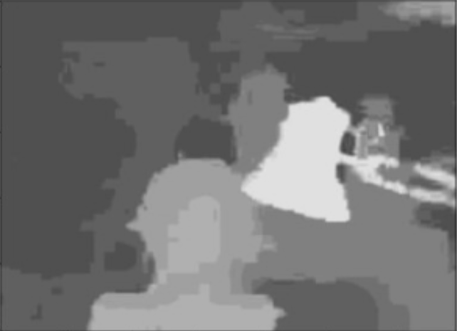
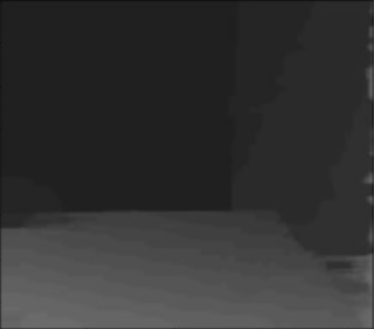
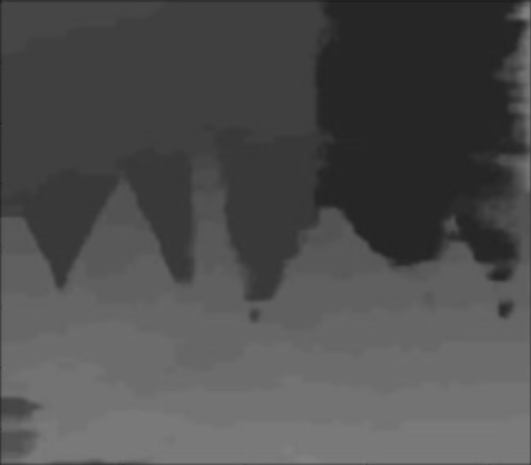
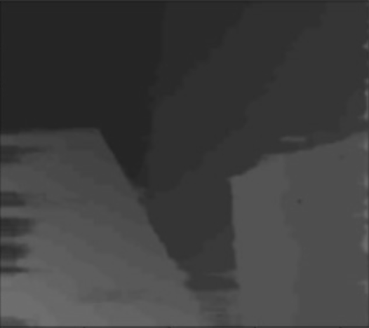
Ours (G)
Heidari (F)

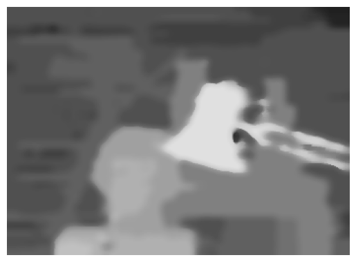
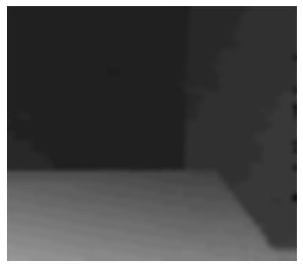
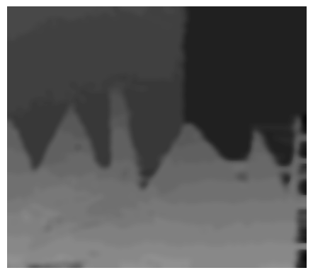
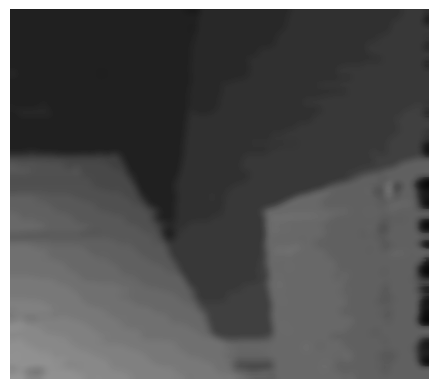
Figure 4: Visual comparison of our method against [26] using Hybrid annealing, and a comparison of our method using Gurobi and the method used in [26] optimized using the classical Ford Fulkerson algorithm [20]. For both methods, we can see a marked visual improvement when classical optimizers are used. Gurobi provides a near-optimal solution, while Ford Fulkerson provides a global optimum.

Image Pair Ours (H) Heidari (H) Ours (G) Heidari (F) RMSE BPP RMSE BPP RMSE BPP RMSE BPP Tsukuba 1.79 26.82 1.8 12.8 1.53 12.93 1.58 13.02 Bull 1.66 31.57 1.3 5.4 0.58 3.46 0.56 3.57 Sawtooth 2.71 47.49 1.9 9.9 1.89 24.51 1.76 11.73 Venus 2.16 42.43 1.4 9.8 0.96 8.16 1.17 10.25 Average 2.06 37.08 1.6 9.48 1.24 12.27 1.27 9.40

Table 2: The Root Mean Squared Error (RMSE) and Bad Pixel Percentage (BPP) of our method against [26] using Hybrid annealing, and a comparison of our method using Gurobi and the method used in [26] optimized using the classical Ford Fulkerson algorithm. Under hybrid annealing conditions, the previous method outperforms ours. Under ideal conditions, we can achieve a lower average RMSE, although we have a higher BPP.

4.3 Comparison to Traditional Methods

We also compared our results against non-quantum classical methods assessed in [26], i.e., Block Matching, [21], Belief Propagation [53], and Local-Expansion [55]. The numerical results are given in Tab. 3 and we can see that with an ideal quantum computer, our approach can outperform existing traditional methods.

Image Pair Ours (G) BM BP LE RMSE BPP RMSE BPP RMSE BPP RMSE BPP Tsukuba 1.53 12.93 1.74 13 1.66 9 1.01 2.9 Bull 0.58 3.46 2.76 23 1.71 8 0.25 0.3 Sawtooth 1.89 24.51 3.34 22 1.96 10 0.81 2.8 Venus 0.96 8.16 3.27 26 2.40 6 0.62 2.31

Table 3: The Root Mean Squared (RMSE) and Bad Pixel Percentage (BPP) of our method against the purely classical Block Matching, [21], Belief Propagation [53], and Local-Expansion [55]. We can see that only Local Expansion outperforms our method on RMSE. Except for the Sawtooth pair, we are also comparable to BM and BP on BPP.

4.4 Ablation Studies

In this section, we perform ablation studies of the elements of our algorithm. We ran our method without a regularization term, with a linear regularizer as in [26], without bilateral filtering, and without median and bilateral filtering.

These results are given in Fig. 5 and Tab. 4 and provide insights into our method. As expected, when no regularizer is used, the quality drops significantly. Using a linear regularizer instead of our more sophisticated nonlinear regularizer had a small impact on the visual appearance and final outcome. In the case of Bull, it is even slightly lower RMSE than the nonlinear regularizer, although it is still higher on average. We suspect this is due to Bull’s disparities being very homogeneous and linear overall, therefore a linear regularizer is advantageous. The bilateral filtering has a blurring effect on the final outcome. Although removing it leads to a small increase RSME, we observe a decrease in BPP. This trade-off occurs because the bilateral filter assists in averaging out the displacements, which generally makes estimates closer in more homogeneous regions, at the cost of a loss of sharpness (and increasing BPP) around the edges. In contrast, removing bilateral and median filtering leads to a much stronger increase in RMSE. This is because median filtering can prevent small inaccuracies made at coarse levels.

	Tsukuba	Bull	Sawtooth	Venus
Ours (G)
— No R
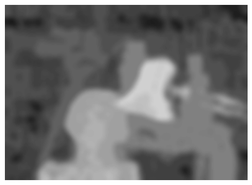
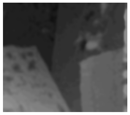
—–L R
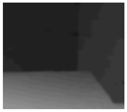
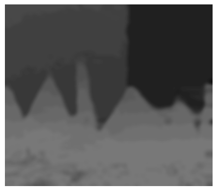
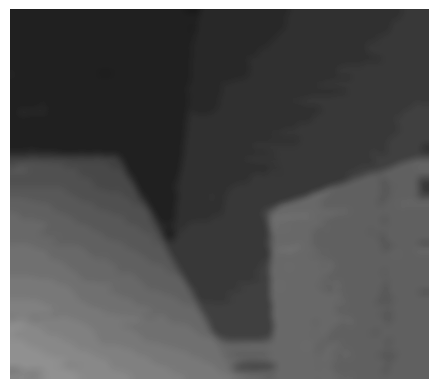
—–No B
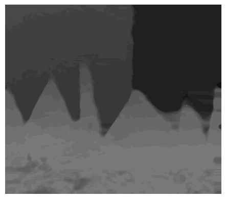
No M No B

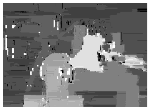
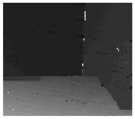
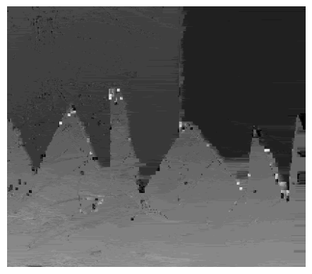
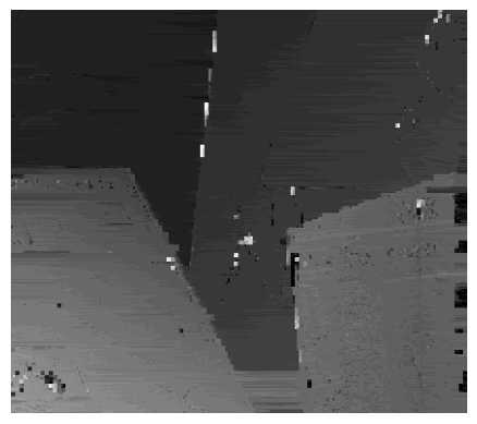
Figure 5: Ablation study of the components of our algorithm. “No Regularizer” sets $E_{s}{=}0$ from line 12 of Algorithm 1, which disables the regularizer and reverts to only using the data term. “Linear Regularizer” does not leverage truncation and is not edge-aware. “No Bilateral filter” removes the bilateral filtering in line 20 of Algorithm 1. “No Median and No Bilateral filtering” row removes lines 18 and 20 from Algorithm 1.

Image Pair Ours (G) No R L R No B No M No B RMSE BPP RMSE BPP RMSE BPP RMSE BPP RMSE BPP Tsukuba 1.53 12.93 1.65 18.63 1.57 13.30 1.59 11.72 2.56 15.19 Bull 0.58 3.46 1.55 16.06 0.56 3.73 0.59 2.70 1.21 6.25 Sawtooth 1.89 24.51 2.30 31.54 1.95 25.20 1.95 23.41 1.99 14.13 Venus 0.96 8.16 1.64 22.22 0.96 7.50 1.03 7.23 1.89 12.34 Average 1.24 12.27 1.79 22.11 1.26 12.43 1.29 11.27 1.91 11.98

Table 4: The RMSE and BPP of our method with different elements removed. See the caption of Fig. 5 for the signification of the abbreviations.

5 Conclusion

We proposed a new approach for quantum-hybrid stereo matching by formulating it as an MRF MAP inference problem. Thanks to the coarse-to-fine policy, we were able to practically apply our technique to real stereo pairs and achieve higher accuracy than prior quantum-admissible stereo matching methods by $2\%$ to $22.5\%$. As more powerful quantum annealers arise in the future and match or surpass the result quality of Gurobi, our method will directly benefit from these improvements.

The QUBO formulation of a general MRF MAP inference allows for greater flexibility in selecting the smoothness term of our energy functional than prior work. Other problems, such as image segmentation and restoration can be expressed as an MRF MAP estimation and are compatible with our technique. Notably, optical flow can be treated as an extension of stereo matching with a 2D search space that could also be estimated by our framework in the future.

Supplementary Material

This supplement contains material which is relevant to our work, but could not be included in the main body of our paper due to the page limit. In Appendix A, we present the formula and proofs for the function $\Lambda(.,.)$ complementing Sec. 3.2 (main paper). In Appendix B, we explain the binary encoding scheme for our MRF as mentioned in Sec. 3.2. In Appendix C, we also offer an analysis of how our QUBO problems embed onto modern quantum hardware, which was also briefly mentioned in Sec. 3.2. In Appendix D, we provide the hyperparameters we used in our algorithm as promised in Sec. 3.3 (main paper). In Appendix E, we ablate our coarse-to-fine method by examining what happens when we remove one intermediate coarse-to-fine step, as we note that each step is necessary in Sec. 3.3. In Appendix F, we examine what happens to our stereo matching results when we lower the values of the rectifier function $\Lambda(.,.)$, as we mention in Sec. 3.2. Finally, in Appendix G, we include additional results of running our algorithm on some examples from the Sintel dataset for stereo matching [9].

Appendix A Deriving Rectifiers For the One-Hot Encoding Scheme

A.1 Deriving Upper Bounds on Non-Granular Rectifiers

We will now derive the function $\Lambda(\ell_{\mathbf{v}}^{r},\ell_{\mathbf{v}}^{s})$, which produces sufficiently high rectifier terms in Eq. 9 such that the QUBO minimizer is the MRF MAP inference. In this section, we define this function such that the constraints are of the form used in QSync [4]. In Sec. A.5, we derive the more granular function. To define $\Lambda(\ell_{\mathbf{v}}^{r},\ell_{\mathbf{v}}^{s})$, we require some additional notation. Suppose $(\mathbf{p},\mathbf{q})\in\mathcal{E}$. Let

$$\gamma(\ell_{\mathbf{p}}^{r},\mathbf{q}):=\text{max}_{\ell_{\mathbf{q}}^{s}\in\mathcal{L}_{\mathbf{q}}}\{\varphi_{\mathbf{p},\mathbf{q}}(\ell_{\mathbf{p}}^{r},\ell_{\mathbf{q}}^{s})\}\,.$$ (15)

Thus, $\gamma(\ell_{\mathbf{p}}^{r},\mathbf{q})$ represents the maximum regularization cost present on the edge $(\mathbf{p},\mathbf{q})$, if $\mathbf{p}$ has been assigned the label $\ell_{\mathbf{p}}^{r}$. Next, we define:

$$\chi(\mathbf{p}):=\text{max}\{0,\text{min}_{\ell_{\mathbf{p}}^{r}\in\mathcal{L}_{\mathbf{p}}}\{\varphi_{\mathbf{p}}(\ell_{\mathbf{p}}^{r})+\sum_{(\mathbf{p},\mathbf{q})\in\mathcal{E}}\text{max}\{0,\gamma(\ell_{\mathbf{p}}^{r},\mathbf{q})\}\}+\epsilon\}\,.\\$$ (16)

$\chi(\mathbf{p})$ is an upper bound of the energy increase of flipping a label $\mathbf{x}_{\ell_{\mathbf{p}}^{r}}$ of $\mathbf{p}$ to be $1$. This energy increase is calculated from the data cost of flipping each label, added to the potential highest possible regularization costs of flipping that label. If all labels for $\mathbf{p}$ are set to $0$, one can always pick a label to flip such that that energy increase is less than or equal to $\chi(\mathbf{p})$. We now define

$$\zeta(\ell_{\mathbf{p}}^{r}):=\sum_{(\mathbf{p},\mathbf{q})\in\mathcal{E}}\sum_{\ell_{\mathbf{q}}^{s}\in\mathcal{L}_{\mathbf{q}}}\text{min}\{0,\varphi_{\mathbf{p},\mathbf{q}}(\ell_{\mathbf{p}}^{r},\ell_{\mathbf{q}}^{s})\}\}\,.$$ (17)

This value tracks all negative regularization energy that can be incurred by flipping $\mathbf{x}_{\ell_{\mathbf{p}}^{r}}$ of $\mathbf{p}$ to be $1$. Next, define

$$\Theta(\ell_{\mathbf{p}}^{r},\ell_{\mathbf{p}}^{s}):=\text{min}\{0,\varphi_{\mathbf{p}}(\ell_{\mathbf{p}}^{r})+\zeta(\ell_{\mathbf{p}}^{r})-\epsilon,\varphi_{\mathbf{q}}(\ell_{\mathbf{q}}^{s})+\zeta(\ell_{\mathbf{q}}^{s})-\epsilon\}\,.$$ (18)

This value accounts for the smaller energy decrease of either flipping $\ell_{\mathbf{p}}^{r}$ or $\ell_{\mathbf{p}}^{s}$ to $1$. Now, for any two labels $\ell_{\mathbf{p}}^{i},\ell_{\mathbf{p}}^{j}\in\mathcal{L}_{\mathbf{p}}$, we can define our function $\Lambda(\ell_{\mathbf{p}}^{i},\ell_{\mathbf{p}}^{j})$ as follows:

$$\Lambda(\ell_{\mathbf{p}}^{i},\ell_{\mathbf{p}}^{j}):=\text{max}\{\chi(\mathbf{p}),\text{max}_{\ell_{\mathbf{p}}^{r},\ell_{\mathbf{p}}^{s}\in\mathcal{L}_{\mathbf{p}}}\{-\Theta(\ell_{\mathbf{p}}^{r},\ell_{\mathbf{p}}^{s})\}\}\,.$$ (19)

We will now show that the lowest energy solution to the QUBO with the matrix presented in Eq. 9 must satisfy the constraints presented in Eq. 8.

A.2 Every Variable Receives at Least One Label

This bound ensures that at least one binary label $\mathbf{x}_{\ell_{\mathbf{p}}^{r}}$ is $1$ for every variable $\mathbf{p}$. Assume that all other labels $\mathbf{x}_{\ell_{\mathbf{p}}^{s}}$ of $\mathbf{p}$ are set to $0$. We select a label to flip $\ell_{\mathbf{p}}^{r}$ such that:

$$\ell_{\mathbf{p}}^{r}=\text{argmin}_{\ell_{\mathbf{p}}^{r}\in\mathcal{L}_{\mathbf{p}}}\{\varphi_{\mathbf{p}}(\ell_{\mathbf{p}}^{r})+\sum_{(\mathbf{p},\mathbf{q})\in\mathcal{E}}\text{max}\{0,\gamma(\ell_{\mathbf{p}}^{r},\mathbf{q})\}\}\,.$$ (20)

Let $c$ be the regularization cost incurred by flipping $\ell_{\mathbf{p}}^{r}$ to $1$. Then, the total change in energy caused by flipping $\ell_{\mathbf{p}}^{r}$ is

$$\begin{split}&\varphi_{\mathbf{p}}(\ell_{\mathbf{p}}^{r})+c-\Lambda(\ell_{\mathbf{p}}^{r},\ell_{\mathbf{p}}^{r})\leq\\ &\varphi_{\mathbf{p}}(\ell_{\mathbf{p}}^{r})+c-\chi(\mathbf{p})\leq\\ &\varphi_{\mathbf{p}}(\ell_{\mathbf{p}}^{r})+c-\text{min}_{\ell_{\mathbf{p}}^{r}\in\mathcal{L}_{\mathbf{p}}}\{\varphi_{\mathbf{p}}(\ell_{\mathbf{p}}^{r})+\sum_{(\mathbf{p},\mathbf{q})\in\mathcal{E}}\text{max}\{0,\gamma(\ell_{\mathbf{p}}^{r},\mathbf{q})\}\}-\epsilon\,.\end{split}$$ (21)

By our construction,

$$c\leq\sum_{(\mathbf{p},\mathbf{q})\in\mathcal{E}}\text{max}\{0,\gamma(\ell_{\mathbf{p}}^{r},\mathbf{q})\},$$ (22)

which means

$$\begin{split}\varphi_{\mathbf{p}}(\ell_{\mathbf{p}}^{r})+c\leq\text{min}_{\ell_{\mathbf{p}}^{r}\in\mathcal{L}_{\mathbf{p}}}\{\varphi_{\mathbf{p}}(\ell_{\mathbf{p}}^{r})+\sum_{(\mathbf{p},\mathbf{q})\in\mathcal{E}}\text{max}\{0,\gamma(\ell_{\mathbf{p}}^{r},\mathbf{q})\}\}\,.\\ \end{split}$$ (23)

Therefore, the expression (21) must be less than or equal to $-\epsilon<0$. Thus, there is still a lower energy to set $\mathbf{x}_{\ell_{\mathbf{p}}^{r}}=1$ rather than $0$.

A.3 Every Variable Receives at Most One Label

Conversely, this bound ensures that at most one label $\mathbf{x}_{\ell_{\mathbf{p}}^{r}}$ is set to $1$ for a variable $\mathbf{p}$. Suppose $\mathbf{x}_{\ell_{\mathbf{p}}^{r}}$ and $\mathbf{x}_{\ell_{\mathbf{p}}^{s}}$ are two binary labels of the same variable. Assume without loss of generality that $\mathbf{x}_{\ell_{\mathbf{p}}^{r}}=1$ and $\mathbf{x}_{\ell_{\mathbf{p}}^{s}}=0$. Now, consider the total change in energy that will occur if we flip $\mathbf{x}_{\ell_{\mathbf{p}}^{s}}$ to $1$: there will be the cost incurred by the diagonal entry of $Q$ ($\varphi_{\mathbf{p}}(\ell_{\mathbf{p}}^{s})-\Lambda(\ell_{\mathbf{p}}^{s},\ell_{\mathbf{p}}^{s})$), the cost of incurred by setting $\mathbf{x}_{\ell_{\mathbf{p}}^{r}}$ and $\mathbf{x}_{\ell_{\mathbf{p}}^{s}}$ to $1$ ($2\Lambda(\ell_{\mathbf{p}}^{s},\ell_{\mathbf{p}}^{r})$), and some regularization cost from neighbor variables, which we will write as $c$. We sum all of these terms together to consider the total change in energy:

$$\begin{split}&\varphi_{\mathbf{p}}(\ell_{\mathbf{p}}^{s})-\Lambda(\ell_{\mathbf{p}}^{s},\ell_{\mathbf{p}}^{s})+2\Lambda(\ell_{\mathbf{p}}^{s},\ell_{\mathbf{p}}^{r})+c=\\ &\varphi_{\mathbf{p}}(\ell_{\mathbf{p}}^{s})+\Lambda(\ell_{\mathbf{p}}^{s},\ell_{\mathbf{p}}^{s})+c\geq\\ &\varphi_{\mathbf{p}}(\ell_{\mathbf{p}}^{s})+\text{max}_{\ell_{\mathbf{p}}^{r},\ell_{\mathbf{p}}^{s}\in\mathcal{L}_{\mathbf{p}}}\{-\Theta(\ell_{\mathbf{p}}^{r},\ell_{\mathbf{p}}^{s})\}+c\geq\\ &\varphi_{\mathbf{p}}(\ell_{\mathbf{p}}^{s})-\Theta(\ell_{\mathbf{p}}^{r},\ell_{\mathbf{p}}^{s})+c=\\ &\varphi_{\mathbf{p}}(\ell_{\mathbf{p}}^{s})-\text{min}\{0,\varphi_{\mathbf{p}}(\ell_{\mathbf{p}}^{r})+\zeta(\ell_{\mathbf{p}}^{r})-\epsilon,\varphi_{\mathbf{p}}(\ell_{\mathbf{p}}^{s})+\zeta(\ell_{\mathbf{p}}^{s})-\epsilon\}+c=\\ &\varphi_{\mathbf{p}}(\ell_{\mathbf{p}}^{s})+\text{max}\{0,-\varphi_{\mathbf{p}}(\ell_{\mathbf{p}}^{r})-\zeta(\ell_{\mathbf{p}}^{r})+\epsilon,-\varphi_{\mathbf{p}}(\ell_{\mathbf{p}}^{s})-\zeta(\ell_{\mathbf{p}}^{s})+\epsilon\}+c\geq\\ &\varphi_{\mathbf{p}}(\ell_{\mathbf{p}}^{s})-\varphi_{\mathbf{p}}(\ell_{\mathbf{p}}^{s})-\zeta(\ell_{\mathbf{p}}^{s})+\epsilon+c=\\ &-\zeta(\ell_{\mathbf{p}}^{s})+\epsilon+c\,.\end{split}$$ (24)

By the construction of $\zeta(\ell_{\mathbf{p}}^{s})$ in Eq. 17, $\zeta(\ell_{\mathbf{p}}^{s})$ must be less than or equal to $c$. Thus, our expression above is greater than or equal to $\epsilon>0$. Thus, there is a net increase in energy when we set both labels to $1$.

A.4 Proof of Correct QUBO Behaviour

We can guarantee that the lowest energy state satisfies our constraints. To understand this, consider a QUBO solution $\mathbf{x}$ where, for some Markov variable $\mathbf{p}$, all binary variables $\mathbf{x}_{\ell_{\mathbf{p}}^{i}}$ are $0$. Then Sec. A.2 proves that there is a label that can be flipped to $1$ to lower the energy. Therefore, $\mathbf{x}$ must not be the optimal solution. Now, consider a solution $\mathbf{x}$ where $2$ or more binary variables that act as labels for Markov variable $\mathbf{p}$ are set to $1$. A.3 shows that there will be a net energy decrease if one of those variables is flipped to $0$. Therefore, $\mathbf{x}$ cannot be the optimal solution. Therefore, the optimal QUBO solution must obey the constraints in Eq. 8.

Let $\mathbf{x}$ be a QUBO solution which obeys all constraints, and corresponds to a labelling $\ell$. The total energy of the QUBO is:

$$\mathbf{x}^{T}Q\mathbf{x}=E(\ell)-\sum_{\mathbf{p}\in\mathcal{V}}\Lambda(\ell_{\mathbf{p}}^{i},\ell_{\mathbf{p}}^{i})\,,$$ (25)

with $E(\ell)$ as defined in Eq. 4. Because $\sum_{\mathbf{p}\in\mathcal{V}}\Lambda(\ell_{\mathbf{p}}^{i},\ell_{\mathbf{p}}^{i})$ is a constant, it is clear that any solution $\mathbf{x}^{*}$ which minimizes $\mathbf{x}^{T}Q\mathbf{x}$ must therefore minimize $E(\ell_{(.)})$.

A.5 A More Granular Implementation of Constraints

We can treat $\Lambda$ is a function of individual labels:

$$\Lambda(\ell_{\mathbf{p}}^{r},\ell_{\mathbf{p}}^{s})=\begin{cases}\chi(\mathbf{p})&\text{ if }r=s\\ \frac{\chi(\mathbf{p})-\Theta(\ell_{\mathbf{p}}^{r},\ell_{\mathbf{p}}^{s})}{2}&\text{ else }\,.\\ \end{cases}\\$$ (26)

We prove that the resulting QUBO obeys our constraints at its optimum, and then the rest of the proof follows exactly the derivations in Sec. A.4.

To prove that every variable receives at least one label, the same argument given in Sec. A.2 holds in this case as well. We can show that for every $\mathbf{p}$, there exists a label $\ell_{\mathbf{p}}^{r}$ such that flipping it to $1$ will cause an energy change of $\varphi_{\mathbf{p}}(\ell_{\mathbf{p}}^{r})+c-\chi(\mathbf{p})<0$ if no other label has been flipped yet.

To prove that every variable receives at most one label, the argument given in Sec. A.3 needs to be modified slightly. In this case, the net change in energy from flipping $\mathbf{x}_{\ell_{\mathbf{p}}^{2}}$ to $1$ is:

$$\begin{split}&\varphi_{\mathbf{p}}(\ell_{\mathbf{p}}^{s})-\chi(\mathbf{p})+2\frac{\chi(\mathbf{p})-\Theta(\ell_{\mathbf{p}}^{r},\ell_{\mathbf{p}}^{s})}{2}+c=\\ &\varphi_{\mathbf{p}}(\ell_{\mathbf{p}}^{s})-\Theta(\ell_{\mathbf{p}}^{r},\ell_{\mathbf{p}}^{s})+c\,.\\ \end{split}$$ (27)

From here, the proof follows the same logic as in Eq. 24.

A.6 Analysis of Improvement

The decrease in $\Lambda(\ell_{\mathbf{p}}^{r},\ell_{\mathbf{p}}^{s})$ for $r=s$ is:

$$\text{max}\{0,\text{max}_{\ell_{\mathbf{p}}^{r},\ell_{\mathbf{p}}^{s}\in\mathcal{L}_{\mathbf{p}}}\{-\Theta(\ell_{\mathbf{p}}^{r},\ell_{\mathbf{p}}^{s})\}-\chi(\mathbf{p})\}\,.$$ (28)

The decrease in $\Lambda(\ell_{\mathbf{p}}^{r},\ell_{\mathbf{p}}^{s})$ for $r\neq s$ is:

$$\text{max}\bigg{\{}\frac{\chi(\mathbf{p})+\Theta(\ell_{\mathbf{p}}^{r},\ell_{\mathbf{p}}^{s})}{2},\text{max}_{\ell_{\mathbf{p}}^{r},\ell_{\mathbf{p}}^{s}\in\mathcal{L}_{\mathbf{p}}}\{-\Theta(\ell_{\mathbf{p}}^{r},\ell_{\mathbf{p}}^{s})\}-\frac{\chi(\mathbf{p})-\Theta(\ell_{\mathbf{p}}^{r},\ell_{\mathbf{p}}^{s})}{2}\bigg{\}}\,.$$ (29)

By implementing more granular constraints, we can be less disruptive to the energy landscape with the same constraint guarantees. Thus, this formulation is an improvement upon the less granular formulation presented in [4]

Appendix B The Binary Encoding of MRF MAP Inference

B.1 Encoding the MRF Energy as a High-Order Binary Polynomial

Let $\operatorname{deg}(\mathbf{p})$ represent the degree of variable $\mathbf{p}$, that is, how many variables are neighbors of $\mathbf{p}$, and define:

$$f_{\mathbf{p},\mathbf{q}}(\ell_{\mathbf{p}},\ell_{\mathbf{q}})=\frac{\varphi_{\mathbf{p}}(\ell_{\mathbf{p}})}{\operatorname{deg}(\mathbf{p})}+\varphi_{\mathbf{p},\mathbf{q}}(\ell_{\mathbf{p}},\ell_{\mathbf{q}})+\frac{\varphi_{\mathbf{q}}(\ell_{\mathbf{q}})}{\operatorname{deg}(\mathbf{q})}\,.$$ (30)

We can view the Markov cost function Eq. 2 from a different perspective:

$$E(\ell_{(\cdot)})=\sum_{(\mathbf{p},\mathbf{q})\in\mathcal{E}}f_{\mathbf{p},\mathbf{q}}(\ell_{\mathbf{p}},\ell_{\mathbf{q}})\,.$$ (31)

For every Markov variable $\mathbf{p}$, we define our label space to be $\mathcal{L}_{\mathbf{p}}=\{0,1\}^{n}$, and we define binary variables $\{\mathbf{x}_{\mathbf{p},0},...,\mathbf{x}_{\mathbf{p},n}\}$. Each $\mathbf{x}_{\mathbf{p},i}$ is flipped to $0$ or $1$, and the sequence $\mathbf{x}_{\mathbf{p},0},...,x_{\mathbf{p},n}$ is a binary encoding of a label in $\mathcal{L}_{\mathbf{p}}$. For label spaces whose size is not a power of $2$, we include extra labels to round the size up to the nearest power of $2$. The extra labels can be duplicates of the original labels.

We will now represent $f_{\mathbf{p},\mathbf{q}}$ as a polynomial of the binary variables $\{\mathbf{x}_{\mathbf{p},0},...,\mathbf{x}_{\mathbf{p},n}\}$, and $\{\mathbf{x}_{\mathbf{q},0},...,\mathbf{x}_{\mathbf{q},m}\}$. To construct this polynomial, we require the following notation: Let $(\sigma_{\mathbf{p}})_{i}$ be the $i^{\text{th}}$ entry of the binary string $\sigma_{\mathbf{p}}\in\mathcal{\mathbf{p}}$. Define:

$$\begin{split}\delta(\sigma_{\mathbf{p}},\mathbf{x}_{\mathbf{p},i})=\begin{cases}\mathbf{x}_{\mathbf{p},i}&\text{if }(\sigma_{\mathbf{p}})_{i}=1\\ 1,&\text{if }(\sigma_{\mathbf{p}})_{i}=0\,.\end{cases}\end{split}$$ (32)

Then, $f_{\mathbf{p},\mathbf{q}}$ is a polynomial of the following form:

$$f_{\mathbf{p},\mathbf{q}}(\mathbf{x}_{\mathbf{p},0},...,\mathbf{x}_{\mathbf{p},n},\mathbf{x}_{\mathbf{q},0},...,\mathbf{x}_{\mathbf{p},m})=\sum_{(\sigma_{\mathbf{p}},\sigma_{\mathbf{q}})\in\mathcal{L}_{\mathbf{p}}\times\mathcal{L}_{\mathbf{q}}}a_{\sigma_{\mathbf{p}},\sigma_{\mathbf{q}}}(\Pi_{i\in[1,...,n]}\delta(\sigma_{\mathbf{p}},\mathbf{x}_{\mathbf{p},i}))\cdot(\Pi_{j\in[1,...,m]}\delta(\sigma_{\mathbf{q}},\mathbf{x}_{\mathbf{q},j}))\,.$$ (33)

where the formula for $a_{\sigma_{\mathbf{p}},\sigma_{\mathbf{q}}}$ is defined as follows: We order $\sigma^{\prime}_{\mathbf{p}}\leq\sigma_{\mathbf{p}}$, if for every index $i$, $(\sigma^{\prime}_{\mathbf{p}})_{i}\leq(\sigma_{\mathbf{p}})_{i}$. Additionally, we define $\kappa(\sigma_{\mathbf{p}})$ to be equal to the number of $1$’s present in $\kappa(\sigma_{\mathbf{p}})$. We can write $a_{\sigma_{\mathbf{p}},\sigma_{\mathbf{q}}}$ as:

$$a_{\sigma_{\mathbf{p}},\sigma_{\mathbf{q}}}:=\sum_{\sigma^{\prime}_{\mathbf{p}}\leq\sigma_{\mathbf{p}},\sigma^{\prime}_{\mathbf{q}}\leq\sigma_{\mathbf{q}}}(-1)^{\kappa(\sigma_{\mathbf{p}})+\kappa(\sigma_{\mathbf{q}})-\kappa(\sigma^{\prime}_{\mathbf{p}})-\kappa(\sigma^{\prime}_{\mathbf{q}})}f_{\mathbf{p},\mathbf{q}}(\sigma^{\prime}_{\mathbf{p}},\sigma^{\prime}_{\mathbf{q}})\,.$$ (34)

We now prove that this formula provides the correct coefficients for our polynomial.

B.2 Proof of Coefficient Formula Correctness

If we plug in the binary strings $\mathbf{x}_{\mathbf{p}}\equiv\mathbf{x}_{\mathbf{p},0},...,\mathbf{x}_{\mathbf{p},n}$ and $\mathbf{x}_{\mathbf{q}}\equiv\mathbf{x}_{\mathbf{q},0},...,\mathbf{x}_{\mathbf{p},m}$ into Eq. 33, we obtain:

$$\begin{split}f_{\mathbf{p},\mathbf{q}}(x_{\mathbf{p}},x_{\mathbf{q}})&=\sum_{\sigma_{\mathbf{p}}\leq x_{\mathbf{p}},\sigma_{\mathbf{q}}\leq x_{\mathbf{q}}}a_{\sigma_{\mathbf{p}},\sigma_{\mathbf{q}}}\\ &=\sum_{\sigma_{\mathbf{p}}\leq x_{\mathbf{p}},\sigma_{\mathbf{q}}\leq x_{\mathbf{q}}}\sum_{\sigma^{\prime}_{\mathbf{p}}\leq\sigma_{\mathbf{p}},\sigma^{\prime}_{\mathbf{q}}\leq\sigma_{\mathbf{q}}}(-1)^{\kappa(\sigma_{\mathbf{p}})+\kappa(\sigma_{\mathbf{q}})-\kappa(\sigma^{\prime}_{\mathbf{p}})-\kappa(\sigma^{\prime}_{\mathbf{q}})}f_{\mathbf{p},\mathbf{q}}(\sigma^{\prime}_{\mathbf{p}},\sigma^{\prime}_{\mathbf{q}})\\ &=\sum_{\sigma^{\prime}_{\mathbf{p}}\leq x_{\mathbf{p}},\sigma^{\prime}_{\mathbf{q}}\leq x_{\mathbf{q}}}f_{\mathbf{p},\mathbf{q}}(\sigma^{\prime}_{\mathbf{p}},\sigma^{\prime}_{\mathbf{q}})\sum_{\sigma^{\prime}_{\mathbf{p}}\leq\sigma_{\mathbf{p}}\leq x_{\mathbf{p}},\sigma^{\prime}_{\mathbf{q}}\leq\sigma_{\mathbf{q}}\leq x_{\mathbf{q}}}(-1)^{\kappa(\sigma_{\mathbf{p}})+\kappa(\sigma_{\mathbf{q}})-\kappa(\sigma^{\prime}_{\mathbf{p}})-\kappa(\sigma^{\prime}_{\mathbf{q}})}\,.\end{split}$$ (35)

We now focus on simplifying the inner term:

$$\begin{split}\sum_{\sigma^{\prime}_{\mathbf{p}}\leq\sigma_{\mathbf{p}}\leq x_{\mathbf{p}},\sigma^{\prime}_{\mathbf{q}}\leq\sigma_{\mathbf{q}}\leq x_{\mathbf{q}}}(-1)^{\kappa(\sigma_{\mathbf{p}})+\kappa(\sigma_{\mathbf{q}})-\kappa(\sigma^{\prime}_{\mathbf{p}})-\kappa(\sigma^{\prime}_{\mathbf{q}})}\,.\end{split}$$ (36)

We can regroup this sum into terms with different values of $\kappa(\sigma^{\prime}_{\mathbf{p}})+\kappa(\sigma^{\prime}_{\mathbf{q}})$. From combinatorics, we know that there are exactly $\binom{\kappa(x_{\mathbf{p}})+\kappa(x_{\mathbf{q}})-\kappa(\sigma^{\prime}_{\mathbf{p}})-\kappa(\sigma^{\prime}_{\mathbf{q}})}{k-\kappa(\sigma^{\prime}_{\mathbf{p}})-\kappa(\sigma^{\prime}_{\mathbf{q}})}$ pairs of binary strings $\sigma_{\mathbf{p}}$, $\sigma_{\mathbf{q}}$ such that $\kappa(\sigma_{\mathbf{p}})+\kappa(\sigma_{\mathbf{q}})=k$. Therefore, we can express Eq. 36 as:

$$\sum_{\kappa(\sigma^{\prime}_{\mathbf{p}})+\kappa(\sigma^{\prime}_{\mathbf{q}})\leq k\leq\kappa(x_{\mathbf{p}})+\kappa(x_{\mathbf{q}})}\binom{\kappa(x_{\mathbf{p}})+\kappa(x_{\mathbf{q}})-\kappa(\sigma^{\prime}_{\mathbf{p}})-\kappa(\sigma^{\prime}_{\mathbf{q}})}{k-\kappa(\sigma^{\prime}_{\mathbf{p}})-\kappa(\sigma^{\prime}_{\mathbf{q}})}(-1)^{k-\kappa(\sigma^{\prime}_{\mathbf{p}})-\kappa(\sigma^{\prime}_{\mathbf{q}})}\,.$$ (37)

We can shift the indices of this sum by $\kappa(\sigma^{\prime}_{\mathbf{p}})+\kappa(\sigma^{\prime}_{\mathbf{q}})$:

$$\sum_{0\leq k\leq\kappa(x_{\mathbf{p}})+\kappa(x_{\mathbf{q}})-\kappa(\sigma^{\prime}_{\mathbf{p}})-\kappa(\sigma^{\prime}_{\mathbf{q}})}\binom{\kappa(x_{\mathbf{p}})+\kappa(x_{\mathbf{q}})-\kappa(\sigma^{\prime}_{\mathbf{p}})-\kappa(\sigma^{\prime}_{\mathbf{q}})}{k}(-1)^{k}\,.$$ (38)

Next, we multiply this term by $1^{\kappa(x_{\mathbf{p}})+\kappa(x_{\mathbf{q}})-\kappa(\sigma^{\prime}_{\mathbf{p}})-\kappa(\sigma^{\prime}_{\mathbf{q}})-k}\equiv 1$ and obtain:

$$\sum_{0\leq k\leq\kappa(x_{\mathbf{p}})+\kappa(x_{\mathbf{q}})-\kappa(\sigma^{\prime}_{\mathbf{p}})-\kappa(\sigma^{\prime}_{\mathbf{q}})}\binom{\kappa(x_{\mathbf{p}})+\kappa(x_{\mathbf{q}})-\kappa(\sigma^{\prime}_{\mathbf{p}})-\kappa(\sigma^{\prime}_{\mathbf{q}})}{k}(-1)^{k}1^{\kappa(x_{\mathbf{p}})+\kappa(x_{\mathbf{q}})-\kappa(\sigma^{\prime}_{\mathbf{p}})-\kappa(\sigma^{\prime}_{\mathbf{q}})-k}\,.$$ (39)

By the binomial theorem, this is equivalent to:

$$(-1+1)^{\kappa(x_{\mathbf{p}})+\kappa(x_{\mathbf{q}})-\kappa(\sigma^{\prime}_{\mathbf{p}})-\kappa(\sigma^{\prime}_{\mathbf{q}})}\,.$$ (40)

If $\sigma^{\prime}_{\mathbf{p}}=x_{\mathbf{p}}$ and $\sigma^{\prime}_{\mathbf{q}}=x_{\mathbf{q}}$, this expression is $1$, and $0$ otherwise. Therefore, we can evaluate the last expression in Eq. 33 to be equal to $f_{\mathbf{p},\mathbf{q}}(x_{\mathbf{p}},x_{\mathbf{q}})$, as needed. This completes the proof. Therefore, if we could somehow transform the minimization of

$$E(\ell_{(\cdot)})=\sum_{(\mathbf{p},\mathbf{q})\in\mathcal{E}}\sum_{(\sigma_{\mathbf{p}},\sigma_{\mathbf{q}})\in\mathcal{L}_{\mathbf{p}}\times\mathcal{L}_{\mathbf{q}}}a_{\sigma_{\mathbf{p}},\sigma_{\mathbf{q}}}(\Pi_{i\in[1,...,n]}\delta(\sigma_{\mathbf{p}},x_{\mathbf{p},i}))\cdot(\Pi_{j\in[1,...,m]}\delta(\sigma_{\mathbf{q}},x_{\mathbf{q},j})),$$ (41)

into the minimization of a quadratic polynomial, we will have formed a QUBO problem.

B.3 Transforming Higher-Order Binary Vector Polynomial Minimization into a QUBO

A technique to transform higher-order polynomial minimization over a binary vector into a QUBO exists and is well explained in Ishikawa [28]: In Sec. 4.2, it is shown that, in a polynomial minimization problem in which all variables are binary, a polynomial term

$$a\mathbf{x}_{0}...\mathbf{x}_{k}$$ (42)

can be transformed into

$$\text{min}_{w\in\{0,1\}}aw\{S_{1}-(k-1)\},$$ (43)

when $a<0$ and

$$\text{min}_{w_{0},...w_{\lfloor\frac{k-1}{2}\rfloor}\in\{0,1\}}a\{\sum_{i=1}^{k}w_{i}(c_{i,k}(-S_{1}+2i)-1)+aS_{2}\},$$ (44)

when $a>0$, and the minimal argument of the polynomial remains the same. Here, $c_{i,k}=1$ if $k$ is odd and $i=k$, and $c_{i,k}=2$ otherwise. $S_{1}$ and $S_{2}$ are defined as:

$$S_{1}=\sum_{i=1}^{k}\mathbf{x}_{i}\,\,\mathrm{and}$$ (45)

$$S_{2}=\frac{S_{1}(S_{1}-1)}{2}\,.$$ (46)

This construction introduces auxiliary binary variables ($w$ if $a<0$ or $w_{1},...,w_{k}$ if $a>0$) to handle the complexity of higher-order terms. These auxiliary binary variables are added into our QUBO problem, and must be optimized alongside our original binary variables. However, once the optimization is complete, we can read off our solution from the original variables and discard the response of the auxiliary variables.

With these techniques, minimization of a polynomial of binary variables of any order can be reduced to a minimization of a quadratic polynomial of binary variables by iteratively applying the transformations explained above to any terms of order greater than $2$. A full proof of why these transformations preserve the minimal argument of the polynomial is too long to explain here, but is elaborated on at length in Ishikawa [28].

We have shown how to express the minimization of $E(\ell_{(\cdot)})$ as a minimization over binary variables. A sketch of the full encoding algorithm goes as follows: 1) For each edge $(\mathbf{p},\mathbf{q})$, calculate all $a_{\mathbf{p},\mathbf{q}}$ from Eq. 34; 2) sum all $f_{\mathbf{p},\mathbf{q}}$ into one large polynomial $E(\ell_{(\cdot)})$ (See Eq. 31), and reduce all higher-order terms to quadratic or lower using the techniques in Ishikawa [28]; 3) build $Q$ from the resulting coefficients.

Appendix C Embedding QUBO Problem Graphs onto D-Wave

One key bottleneck for modern quantum computing is minor embedding: once a QUBO is defined, all the binary variables of $\mathbf{x}$ must be mapped to physical qubits present on the QPU, and all non-zero entries of the off-diagonals of $Q$ must be mapped to the appropriate physical couplers connecting physical qubits. To make this embedding process more flexible, it is possible to chain qubits together: any two physical qubits which share a coupler can be treated as a single physical qubit during the embedding. However, during annealing, qubit chains are at risk of breaking (i.e., not behaving like a single physical qubit), making it ill-defined to measure the QUBO solution from the annealer. The longer the qubit chain, the higher the risk of the chain breaking. Therefore, we aim to keep chains as small as possible.

We first examine the embedding properties of our one-hot encoding scheme, and then turn our attention to the binary encoding scheme proposed in Appendix B, and see why it is more challenging to embed.

C.1 Embedding of the One-Hot Encoding Scheme

A QUBO’s problem graph is a useful concept for discussing minor embedding. For a QUBO problem represented by the matrix $Q$, the corresponding problem graph has vertices corresponding to each binary variable of the QUBO, and edges connecting any two vertices whose corresponding binary variables interact in the QUBO problem. We visualize the QUBO problem graphs for the first epipolar line of the Venus image pair at all three coarse-to-fine steps in Fig. 6. We visualize those same problem graphs when they are embedded onto the D-Wave Pegasus hardware in Fig. 7. The numerics for these problem graphs and embeddings are given in Tab. 5.

For all steps, an embedding is possible, meaning our algorithm can be run on modern hardware. Additionally, the number of vertices of our QUBO problem graph grows linearly as the number of disparities considered by the algorithm increases, or when the length of the epipolar line increases. This means that the one-hot encoding scales well as our problem size increases.

Step 1	Step 2	Step 3

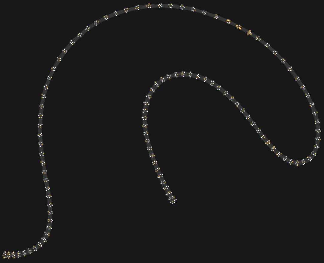
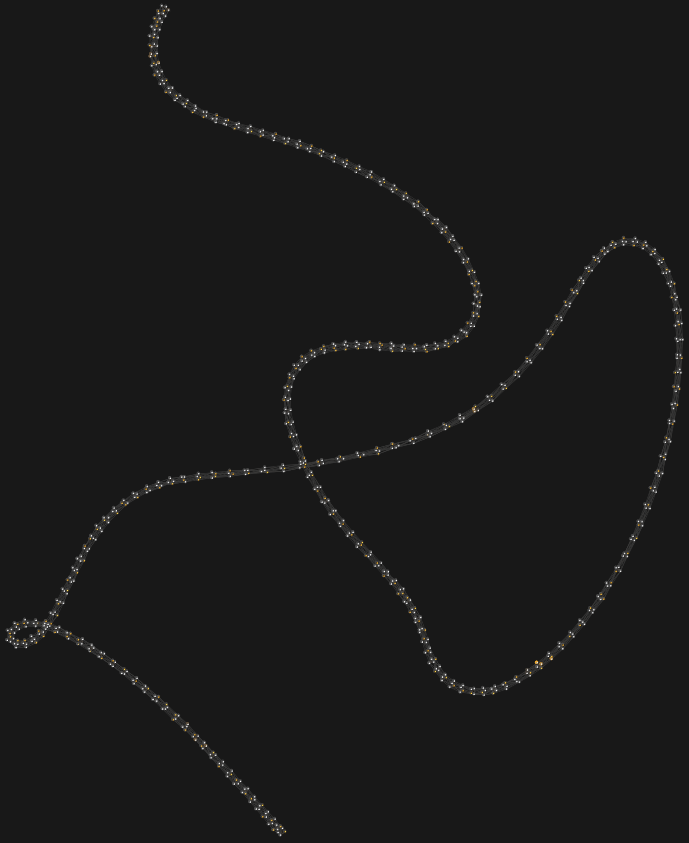
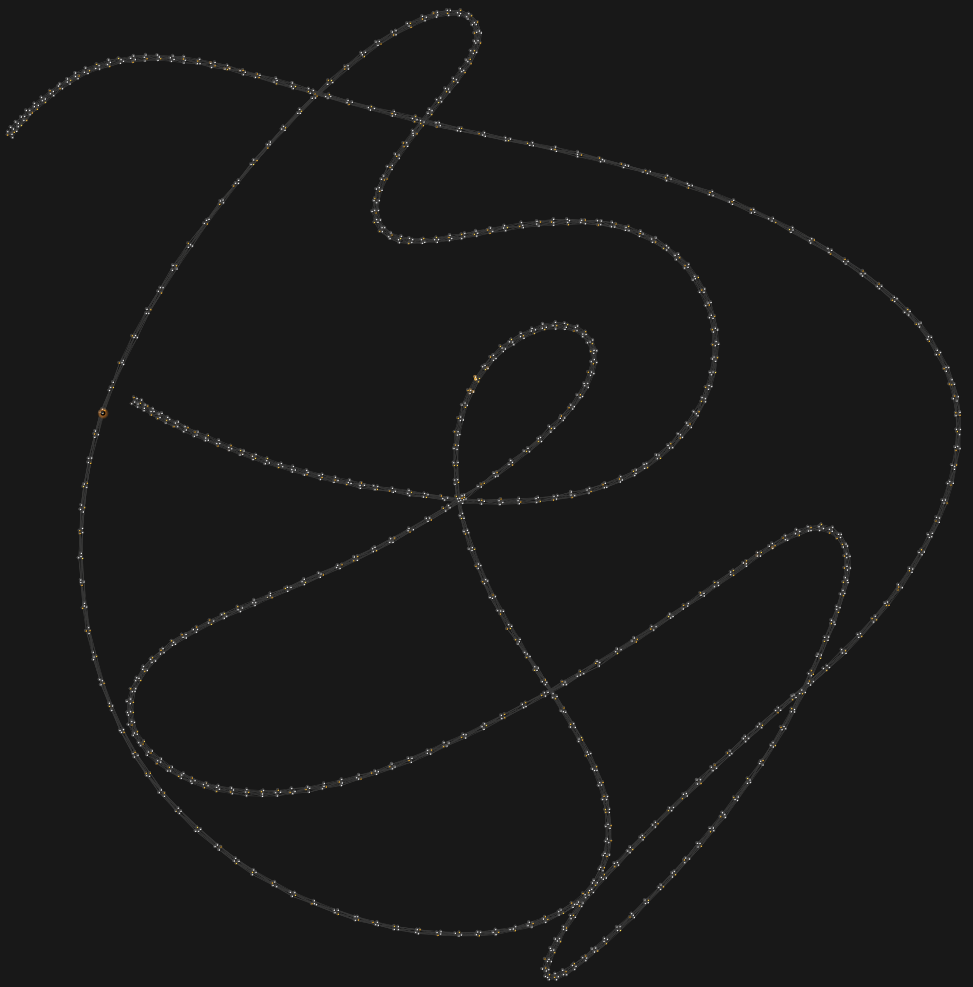
Figure 6: The QUBO problem graphs for the first epipolar line of Venus image pair visualized using D-Wave’s Problem Inspector. The single curve structure of these graphs arises because regularization costs only occur between the immediate neighbors on the epipolar line.

Step 1	Step 2	Step 3

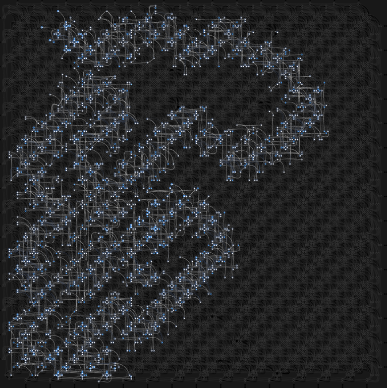
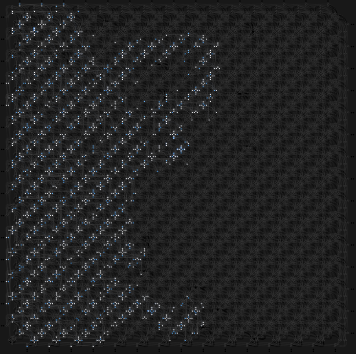
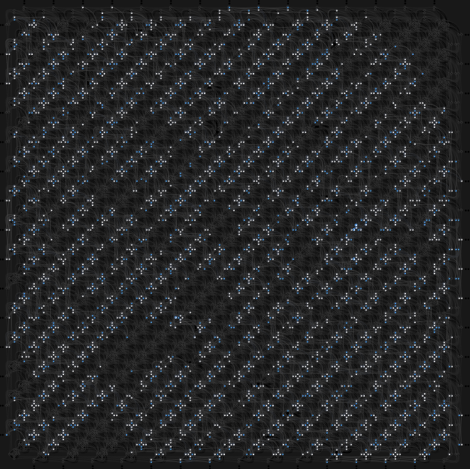
Figure 7: The QUBO problem embeddings onto D-Wave’s Pegasus QPU for the first epipolar line of Venus image pair visualized using D-Wave’s Problem Inspector. The Pegasus QPU has $5,640$ qubits with $40,484$ couplers [6]. Although the QUBO problem graphs have much fewer vertices and edges than the Pegasus QPU’s qubits and couplers, one can see that a large portion of these resources are needed in order to embed properly. This is because many qubit chains are used for the embedding.

Step	1	2	3
Epipolar Line Length	108	217	434
Disparity Levels	6	4	4
QUBO Graph Nodes	648	868	1,736
QUBO Graph Edges	5,472	4,758	9,532
Physical Qubits	2,254	1,937	3,795
Physical Couplers	6,541	5,827	11,591
Physical Max Chain Length	10	5	5

Table 5: QUBO Problem graph statistics for our method with a one-hot encoding scheme for a single epipolar line, and statistics on the computed embeddings of the QUBO problem graphs onto the D-Wave Pegasus QPU. The epipolar line length is from the widest of the Middlebury images, Venus and Sawtooth. Thus, our stereo matching QUBO problems are embeddable on modern quantum hardware.

C.2 Embedding of the Binary Encoding Scheme

We report the number of QUBO problem graph edges and vertices required for stereo matching the Venus image pair (across all steps) in Tab. 6. For Step 1, the number of edges is greater than the number of couplers, meaning it is impossible to find an embedding. As the number of disparities grows, the number of auxiliary binary variables needed grows exponentially (see Section 5.4 of Ishikawa [28]). This explains why the problem graph for the initial step is so large. Note that the number of binary variables needed still grows linearly with respect to epipolar line length.

D-Wave’s upcoming QPU with the Zephyr topology (expected in 2024) should contain $7.4\cdot 10^{4}$ qubits [13]. However, we were still unable to find an embedding for Step 1 in this topology. Because we cannot embed this binary encoding approach into modern or next-generation QPU’s, we decided to focus our attention on using the one-hot encoding scheme.

Step	1	2	3
QUBO Graph Nodes	5,461	1,514	3,033
QUBO Graph Edges	147,452	7,561	15,156

Table 6: Computed embeddings for the D-Wave Pegasus, binary encoding. Given the increased complexity of the graph topology, we were unable to calculate embeddings for all $3$ resolution levels.

Appendix D Model Hyperparameters

We summarize our model parameters used across all three coarse-to-fine levels of our algorithm in Tab. 7. These parameters were found to optimize RMSE while keeping an acceptable BPP. The median filter is across an entire window – and not a vertical median filter as in [26] – as we found this improved the estimation. We found that at the full resolution, a non-truncated regularizer worked best in general. Nevertheless, we still leverage the truncation at lower levels, so it is still present in our approach. Also, note that the range of $I^{L},I^{R}$ is on the interval $[0,1]$.

Step	1	2	3
Downsample Factor (Algorithm 1)	4	2	1
Displacements Considered (Algorithm 1)	6	4	4
$\tau$ (Eq. 11)	0.15	0.15	0.3
q (Eq. 11)	10	10	10
m (Eq. 12)	0.0015	0.0015	$\infty$
s (Eq. 12)	0.0005	0.0003	0.0005
Median Filter Window (Algorithm 1)	7$\times$7	7$\times$7	7$\times$7
Bilateral Filter Diameter (Algorithm 1)	n/a	n/a	12
Bilateral Filter Sigma Color (Algorithm 1)	n/a	n/a	75
Bilateral Filter Sigma Space (Algorithm 1)	n/a	n/a	75

Table 7: Hyperparameters for our stereo matching algorithm described in Sec. 3.4 of the main paper.

Appendix E Ablation Study on the Coarse-to-Fine Levels

We investigated how well our method works if we have fewer coarse-to-fine levels. In the following experiment, we removed the iteration which considers stereo matching at a downsampling factor of $2$ (step $2$). The modified algorithm can still estimate all disparities (rounded to the nearest integer) present in the ground truth, provided that it makes the correct estimation at each step. The visual results as shown in Fig. 8 and numerical results are shown in Tab. 8. Other than the Sawtooth image pair, we see a decline visually and numerically in our estimates. We conclude that having intermediate resolution steps is useful to our method. They give the algorithm more opportunities to adjust as higher resolution details are shown, correcting previous inaccuracies. We also suspect that the inaccurate estimates for Sawtooth begin in the second iteration because its omission leads to better numerical results, and the improvement is particularly noticeable in the troublesome lower left area.

Image Pair	AS		NS2
	RMSE	BPP	RMSE	BPP
Tsukuba	1.53	12.93	1.60	13.97
Bull	0.58	3.46	0.82	10.15
Sawtooth	1.89	24.51	1.71	18.06
Venus	0.96	8.16	1.15	13.62
Average	1.24	12.27	1.32	13.95

Table 8: The Root Mean Squared Error (RMSE) and Bad Pixel Percentage (BPP) of our full method with All Steps, and our method when the iteration step at the intermediate resolution is removed (No Step 2). The Gurobi optimizer is used in both cases. The full algorithm has lower RMSE an BPP.

	Tsukuba	Bull	Sawtooth	Venus
————GT
———–AS
————NS2

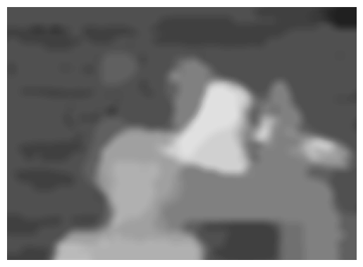
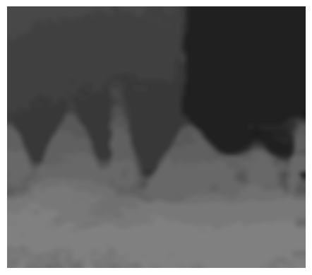
Figure 8: By row: Ground-Truth displacements for each pair, our full method with All Steps, and our method when the iteration step at the intermediate resolution is removed (No Step 2). We can see that removing the second step means that some details are inaccurately estimated, such as a portion of the lamp in Tsukuba and planar regions in Venus. However, in the case of Sawtooth this lack of iterations and attention to details works to the algorithm’s benefit.

Appendix F Ablation Study on the Strength of the Rectifiers

As discussed in Birdal et al. [4], larger constraint values can negatively affect annealer performance. Therefore, we wanted to see if we can improve performance by decreasing these constraint values. What this means in practice is that we modify our QUBO matrix given in Eq. 9 to the following:

$$\begin{split}\forall\mathbf{v}\in\mathcal{V},\,\forall\ell_{\mathbf{v}}^{l}\in\mathcal{L}_{\mathbf{v}}:&\,\,Q_{\ell_{\mathbf{v}}^{l},\ell_{\mathbf{v}}^{l}}=\varphi_{\mathbf{v}}(\ell_{\mathbf{v}}^{l})-t\cdot\Lambda(\ell_{\mathbf{v}}^{l},\ell_{\mathbf{v}}^{l})\\ \forall\mathbf{p}\in\mathcal{V},\,\forall\ell_{\mathbf{p}}^{r},\ell_{\mathbf{p}}^{s}\in\mathcal{L}_{\mathbf{p}},\,r\neq s:&\,\,Q_{\ell_{\mathbf{p}}^{r},\ell_{\mathbf{p}}^{s}}=t\cdot\Lambda(\ell_{\mathbf{p}}^{r},\ell_{\mathbf{p}}^{s})\\ &\,\,Q_{\ell_{\mathbf{p}}^{j},\ell_{\mathbf{p}}^{i}}=t\cdot\Lambda(\ell_{\mathbf{p}}^{r},\ell_{\mathbf{p}}^{s})\\ \forall(\mathbf{p},\mathbf{q})\in E,\forall\ell_{\mathbf{p}}^{i}\in\mathcal{L}_{\mathbf{p}}\forall\ell_{\mathbf{q}}^{j}\in\mathcal{L}_{\mathbf{q}}:&\,\,Q_{\ell_{\mathbf{p}}^{i},\ell_{\mathbf{q}}^{j}}=\frac{1}{2}\varphi_{\mathbf{p},\mathbf{q}}(\ell_{\mathbf{p}}^{i},\ell_{\mathbf{q}}^{j})\\ &\,\,Q_{\ell_{\mathbf{q}}^{j},\ell_{\mathbf{p}}^{i}}=\frac{1}{2}\varphi_{\mathbf{p},\mathbf{q}}(\ell_{\mathbf{p}}^{i},\ell_{\mathbf{q}}^{j}).\\ \end{split}$$ (47)

Here, $t\geq 0$ can adjust the strength of our rectifiers. Our formulation in Eq. 9 is a specialized case of Eq. 47 where $t=1$. For this experiment, we ran our stereo matching algorithm on the four Middlebury image pairs using all the default settings as described in Appendix D, while changing this newly introduced variable $t$. We show the visual results in Fig. 10 and numerical results in Tab. 9. Note that in the case that two or more disparities are chosen during annealing, the lower disparity is chosen. In the case that no disparity was selected, the lowest possible disparity was selected. These experiments ran on D-Wave’s simulated annealer.

By graphing the of the average RMSE and BPP of these stereo estimates over $t$ (as shown in Fig. 9), we observe that lowering $t$ actually improves our results, with an optimum around $t=0.25$, even though for this value, our constraints have not been formally proven to be obeyed. We also observe that some $t>0$ is necessary to avoid the simulator returning the trivial answer of $0$. Given more time, we would like to investigate this performance improvement further to optimize $t$, and conduct experiments on the actual QPU.

Image Pair $t=0$ (SA) $t=0.25$ (SA) $t=0.5$ (SA) $t=0.75$ (SA) $t=1$ (SA) $t=1.25$ (SA) $t=1.5$ (SA) RMSE BPP RMSE BPP RMSE BPP RMSE BPP RMSE BPP RMSE BPP RMSE BPP Tsukuba 7.29 100 1.87 26.24 1.80 23.70 1.79 24.37 1.87 30.64 1.84 27.11 1.89 30.06 Bull 8.29 100 1.30 24.28 1.42 31.59 1.97 38.53 1.87 45.29 2.10 43.74 2.21 48.11 Sawtooth 10.72 100 2.86 38.09 2.84 46.84 2.98 53.85 3.04 56.75 3.23 59.50 3.22 60.96 Venus 9.39 100 2.04 36.73 2.12 42.35 2.26 47.83 2.27 47.73 2.35 50.28 2.56 53.71 Average 8.92 100 2.02 31.34 2.05 36.12 2.25 41.15 2.26 45.10 2.38 45.16 2.47 48.21

Table 9: The Root Mean Squared Error (RMSE) and Bad Pixel Percentage (BPP) of the Simulated Annealing method for increasing values of $t$. Lowering $t$ below $1$ can improve our metrics.

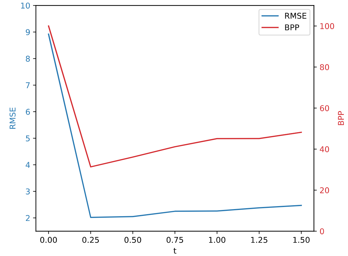
Figure 9: The average RMSE and BPP for the four Middlebury benchmarks over the rectifier strength $t$. We observe that both error metrics obtain a minimum around $t=0.25$.

	Tsukuba	Bull	Sawtooth	Venus
—–.—GT
—-$t=0$ (SA)
–.$t=0.25$ (SA)
—$t=0.5$ (SA)
–.$t=0.75$ (SA)
—-.$t=1$ (SA)
–.$t=1.25$ (SA)
—.$t=1.5$ (SA)

Figure 10: Ground-Truth displacements compared with our Simulated Annealing approach for increasing $t$ values.

Appendix G Sintel Experiments

We ran our model on several stereo image pairs from the Sintel dataset [9]. To account for the larger displacements present in the Sintel data, we adjusted our method to now have six coarse-to-fine levels in total. The full configuration of hyperparameters is given in Tab. 10. Visual results can be found in Fig. 11, and numerical results can be found in Tab. 11. All estimates were done using Gurobi [24].

We observe that our method is capable of scaling up to larger image pairs with more complex scenes. In particular, stereo pairs with a continuous gradient of disparities, such as the walls in Alley 2, are estimated well. The method is also capable of picking out finer details, such as the ladder in the lower left section of Alley 2. At the same time, there are still some challenges. Small errors in coarser iterations compound into larger errors (observe the blotchy artifact in the upper right section of Alley 2, for example). The proposed approach also struggles with precision in detail-heavy foregrounds. For example, the hair in Alley 1 is missing some finer details. We suspect that in this case, the brightness constancy assumption is insufficient, and more advanced data terms could be investigated in the future.

Step	1	2	3	4	5	6
Downsample Factor (Algorithm 1)	32	16	8	4	2	1
Displacements Considered (Algorithm 1)	6	6	6	4	4	4
$\tau$ (Eq. 11)	0.15	0.15	0.15	0.15	0.15	0.3
q (Eq. 11)	10	10	10	10	10	10
m (Eq. 12)	0.0015	0.0015	0.0015	0.0015	0.0015	$\infty$
s (Eq. 12)	0.0005	0.0005	0.0005	0.0005	0.0003	0.0005
Median Filter Window (Algorithm 1)	3$\times$3	3$\times$3	3$\times$3	3$\times$3	3$\times$3	7$\times$7
Bilateral Filter Diameter (Algorithm 1)	n/a	n/a	n/a	n/a	n/a	12
Bilateral Filter Sigma Color (Algorithm 1)	n/a	n/a	n/a	n/a	n/a	75
Bilateral Filter Sigma Space (Algorithm 1)	n/a	n/a	n/a	n/a	n/a	75

Table 10: Hyperparameters for our stereo matching algorithm for the Sintel dataset [9].

	Alley 1	Alley 2	Sleeping 2
——–LI
———GT
——Ours (G)
	Temple 2	Market 2	Sleeping 1
——–LI
———GT
——Ours (G)

Figure 11: The first and fourth rows show the Left Image from the first frame of the selected scenes of the Sintel stereo pairs. The second and fifth rows show the Ground-Truth displacements for each pair. The third and sixth rows show our stereo estimation approach using Gurobi. We observe that our method can still make robust estimates, even though the input data is of higher resolution and more visually complex.

Image Pair	Ours (G)
	RMSE	BPP
Alley 1	38.44	50.21
Alley 2	12.44	23.03
Sleeping 2	3.47	20.23
Temple 2	1.88	10.30
Market 2	10.83	31.22
Sleeping 1	8.73	60.35

Table 11: The Root Mean Squared Error (RMSE) and Bad Pixel Percentage (BPP) of our method using Gurobi on frame pairs from the Sintel dataset.

Appendix H QUBO Matrix Visualization

In this section, we examine the quantum annealing process on the first epipolar line on the Tsukuba image pair at the coarsest resolution. We first visualize the Ising model problem derived from the QUBO problem for stereo matching across this epipolar line. The Ising model problem attempts to minimize the following energy:

$$H(s)=\sum_{i}h_{i}s_{i}+\sum_{i\neq j}J_{i,j}s_{i}s_{j}$$ (48)

where each $s_{i}\in\{-1,1\}$ corresponds to the QUBO variable $\mathbf{x}_{i}$ via the equation:

$$s_{i}=2\mathbf{x}_{i}-1$$ (49)

and each $h_{i}$ is calculated from $Q=\{q_{i,j}\}$ as

$$h_{i}=\frac{q_{ii}}{2}+\sum_{j\neq i}\frac{q_{i,j}+q_{j,i}}{4}$$ (50)

and each $J_{i,j}$ is calculated as

$$J_{i,j}=\frac{q_{i,j}}{4}$$ (51)

The weights from the Ising model problem are directly translated into the QPU component’s energies, therefore by visualizing these weights, one can better understand the energy landscape and topological complexity of the problem. To visualize these weights, we place them into a matrix with the diagonal is populated with $h_{i}$, and the off diagonal is populated with $J_{i,j}$. We then visualize the value of the matrix entries in Fig. 12

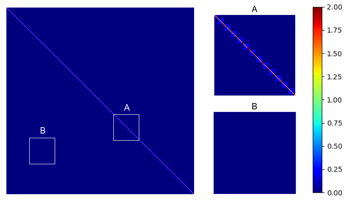
Figure 12: The Ising model matrix’s values visualized with a color mapping. The matrix has an observable pattern of $6\times 6$ submatrices of higher values centered on the diagonal, is shown in the zoomed in section A. Each one of these $6\times 6$ submatrices encodes the energy costs of selecting one of the $6$ possible labels for a particular pixel. The majority of the entries are $0$, as shown in the zoomed in section B. We scaled the entries of this matrix to be in the standard range accepted by the D-Wave QPUs, see [54]. The relative sparseness of the matrix means that it is easier to embed than a denser matrix (See Appendix C for an in-depth discussion on embedding). We also observe that, of the non-zero entries, the highest entries are concentrated on the diagonal, and are significantly higher than other entries. This lack of balance between entries can exacerbate the minimum gap problem.

We also wanted to examine how the minimum gap was affected by the constraints, as we observed better annealing performance with lower constraints. To do so, we looked a small $10$ qubit subproblem from the first epipolar line of the Tsukuba image pair at the coarsest resolution. Beyond $10$ or so qubits makes it impossible to tractably calculate the Hamiltonian’s eigenspectrum (the Hamiltonian grows exponentially with the number of qubits). We plotted the two lowest eigenvalues over time for this problem in Fig. 13 for different constraint weights. We found that the hard constrained problem ($t=1$) had a minimum gap of $0.039$, while the soft constrained problem ($t=0.25$) had a minimum gap of $0.109$. Thus, we can see that the minimum gap problem is lessened when constraints are relaxed. We ran this experiment for the other Middlebury image pairs, see Fig. 14

Hard Constraints	Soft Constraints

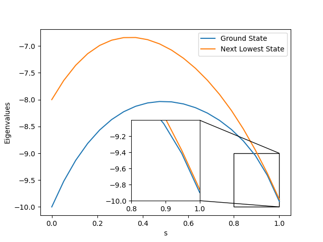
Figure 13: The two lowest value spectral lines of the Hamiltonian as it transitions from its initial state to the final state. We compare between a final problem Hamiltonian which enforces hard constraints ($t=1$), compared with a same final problem Hamiltonian using soft constraints ($t=0.25$), which had better performance on the simulated annealer. In both cases, the minimum gap occurs near the end of the annealing, but we can observe that this gap remains larger in the soft constraint case, which can help explain the improved annealing performance. The near convergence of the spectral lines as the Hamiltonian becomes our problem Hamiltonian also implies that the nature of this problem will be challenging to globally optimize on an annealer, even with softened constraints. Ideally, we would run an eigenspectrum analysis on the full epipolar line problem, however this is not computationally feasible. It is possible that with a larger problem, the difference in minimum gaps would be more pronounced.

Hard Constraints	Soft Constraints

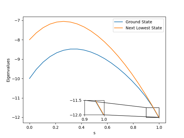
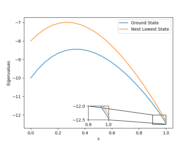
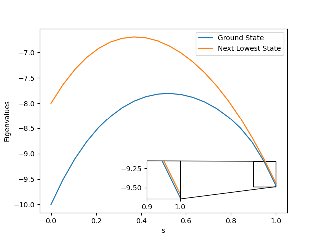
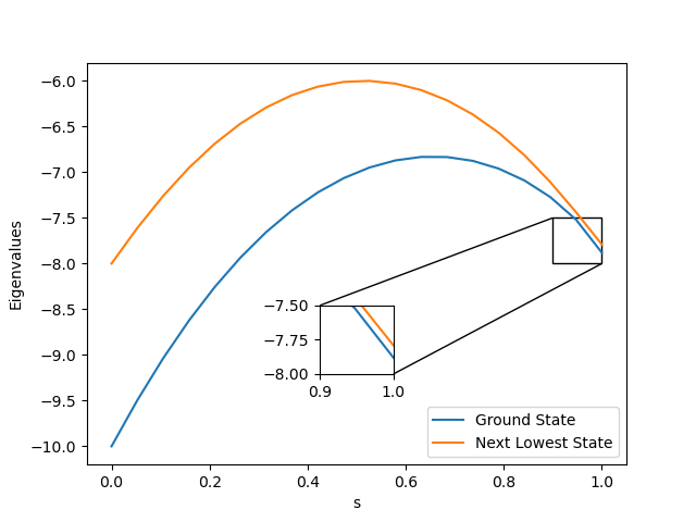
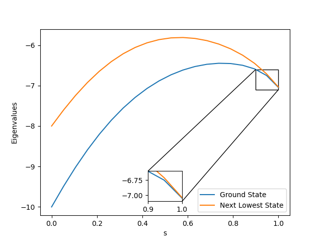
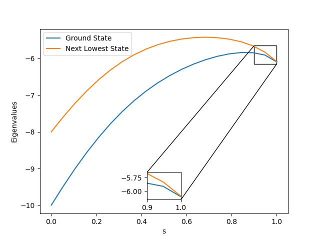
Figure 14: The same experiment as in Fig. 13, only this time we consider the Bull, Sawtooth, and Venus image pairs (presented in that order top to bottom). We see that in all three of these cases, the minimum gap is always smaller in the $t=1$ case than in the $t=0.25$ case. For Bull, the difference is between $0.020$ and $0.119$. For Sawtooth, the difference is between $0.045$ and $0.081$. For Venus, the difference is between $0.001$ and $0.011$. This is further evidence that relaxing constraints shrinks the minimum gap

Appendix I Algorithm Diagrams

We visualize the core of our algorithm in Fig. 15. This shows the image values along the epipolar lines of our images are processed by our algorithm, and ultimately influence the programming of the QPU.

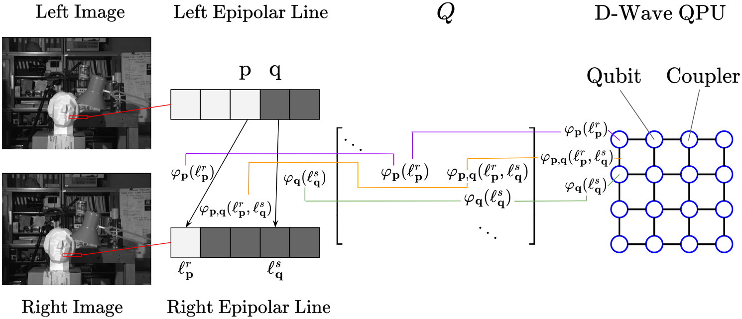
Figure 15: Visualization of Our Algorithm: We zoom in on the corresponding epipolar lines (See Sec. 3.3) for the Tsukuba image pair. For pixels with Markov variables $\mathbf{p}$ and $\mathbf{q}$, we consider their respective displacement labels $\ell_{\mathbf{p}}^{r}$ and $\ell_{\mathbf{q}}^{s}$ (See Sec. 3.2). We classically calculate the data costs $\varphi_{\mathbf{p}}(\ell_{\mathbf{p}}^{r})$ and $\varphi_{\mathbf{q}}(\ell_{\mathbf{q}}^{s})$, and the regularization cost $\varphi_{\mathbf{p},\mathbf{q}}(\ell_{\mathbf{q}}^{s},\ell_{\mathbf{p}}^{r})$. These values are then processed into the QUBO matrix $Q$ (See Sec. 3.1), which is then used to set the qubit and coupler energies on the D-Wave QPU (Also see Sec. 3.1). The diagram only sketches how these cost values calculated from the image pair are programmed into the QPU. Numerical details of the QUBO encoding scheme in $Q$ and minor embedding in the D-Wave QPU have been omitted for the sake of simplicity.

References

- Albash and Lidar [2018] Tameem Albash and Daniel A. Lidar. Demonstration of a scaling advantage for a quantum annealer over simulated annealing. Phys. Rev. X, 8:031016, 2018.
- Arrigoni et al. [2022] Federica Arrigoni, Willi Menapace, Marcel Seelbach Benkner, Elisa Ricci, and Vladislav Golyanik. Quantum motion segmentation. In European Conference on Computer Vision (ECCV), 2022.
- Barnard [1989] Stephen T Barnard. Stochastic stereo matching over scale. International Journal of Computer Vision, 3(1):17–32, 1989.
- Birdal et al. [2021] Tolga Birdal, Vladislav Golyanik, Christian Theobalt, and Leonidas Guibas. Quantum permutation synchronization, 2021.
- Blake and Zisserman [1987] Andrew Blake and Andrew Zisserman. Visual reconstruction. MIT press, 1987.
- Boothby et al. [2020] Kelly Boothby, Paul Bunyk, Jack Raymond, and Aidan Roy. Next-generation topology of d-wave quantum processors. arXiv e-prints, 2020.
- Born and Fock [1928] Max Born and Vladimir Fock. Beweis des adiabatensatzes. Zeitschrift für Physik, 51(3):165–180, 1928.
- Bravyi et al. [2022] Sergey Bravyi, Oliver Dial, Jay M Gambetta, Darío Gil, and Zaira Nazario. The future of quantum computing with superconducting qubits. Journal of Applied Physics, 132(16), 2022.
- Butler et al. [2012] Daniel Jonas Butler, J. Wulff, Garrett B. Stanley, and Michael J. Black. A naturalistic open source movie for optical flow evaluation. In European Conf. on Computer Vision (ECCV), pages 611–625. Springer-Verlag, 2012.
- Cai et al. [2014] Jun Cai, William G. Macready, and Aidan Roy. A practical heuristic for finding graph minors. arXiv, 2014.
- Chou and Brown [1990] Paul B Chou and Christopher M Brown. The theory and practice of bayesian image labeling. International journal of computer vision, 4:185–210, 1990.
- Cruz-Santos et al. [2018] William Cruz-Santos, Salvador Elías Venegas-Andraca, and Marco Lanzagorta. A qubo formulation of the stereo matching problem for d-wave quantum annealers. Entropy, 20, 2018.
- D-Wave [2021] D-Wave. Zephyr topology of d-wave quantum processors (d-wave technical report series). https://www.dwavesys.com/media/2uznec4s/14-1056a-a_zephyr_topology_of_d-wave_quantum_processors.pdf, 2021.
- D-Wave Systems, Inc. [2023] D-Wave Systems, Inc. Simulated annealing sampler. https://github.com/dwavesystems/dwave-neal/blob/master/docs/reference/sampler.rst, 2023. online; accessed on the 07.08.2023.
- Doan et al. [2022] Anh-Dzung Doan, Michele Sasdelli, David Suter, and Tat-Jun Chin. A hybrid quantum-classical algorithm for robust fitting. In Computer Vision and Pattern Recognition (CVPR), pages 417–427, 2022.
- Drory et al. [2014] Amnon Drory, Carsten Haubold, Shai Avidan, and Fred A. Hamprecht. Semi-global matching: A principled derivation in terms of message passing. In German Conference on Pattern Recognition, 2014.
- Farhi et al. [2000] Edward Farhi, Jeffrey Goldstone, Sam Gutmann, and Michael Sipser. Quantum computation by adiabatic evolution. arXiv: Quantum Physics, 2000.
- Farhi et al. [2001] Edward Farhi, Jeffrey Goldstone, Sam Gutmann, Joshua Lapan, Andrew Lundgren, and Daniel Preda. A quantum adiabatic evolution algorithm applied to random instances of an np-complete problem. Science, 292(5516):472–475, 2001.
- Finsterwalder [1897] Sebastian Finsterwalder. Die geometrischen grundlagen der photogrammetrie. Jahresbericht der Deutschen Mathematiker-Vereinigung, 6, 1897.
- Ford and Fulkerson [2010] Lester Randolph Ford and Delbert Ray Fulkerson. Flows in Networks. Princeton University Press, 2010.
- Furht [2008] Borko Furht. Block Matching, pages 55–56. Springer US, Boston, MA, 2008.
- Gennert [1988a] Michael A. Gennert. Brightness-based stereo matching. International Conference on Computer Vision (ICCV), pages 139–143, 1988a.
- Gennert [1988b] Michael A Gennert. Brightness-based stereo matching. In 1988 Second International Conference on Computer Vision, pages 139–140. IEEE Computer Society, 1988b.
- Gurobi Optimization, LLC [2023] Gurobi Optimization, LLC. Gurobi Optimizer Reference Manual, 2023.
- Hauck [1883] Guido Hauck. Neue constructionen der perspective und photogrammetrie. (theorie der trilinearen verwandtschaft ebener systeme, i. artikel.). Journal für die reine und angewandte Mathematik (Crelles Journal), 1883.
- Heidari et al. [2021] Shahrokh Heidari, Mitchell Rogers, and Patrice Delmas. An improved quantum solution for the stereo matching problem. In International Conference on Image and Vision Computing New Zealand (IVCNZ), 2021.
- Hirschmuller [2005] Heiko Hirschmuller. Accurate and efficient stereo processing by semi-global matching and mutual information. In Computer Vision and Pattern Recognition (CVPR), 2005.
- Ishikawa [2011] Hiroshi Ishikawa. Transformation of general binary mrf minimization to the first-order case. IEEE Transactions on Pattern Analysis and Machine Intelligence, 33(6):1234–1249, 2011.
- Kirkpatrick et al. [1983] Scott Kirkpatrick, Daniel Gelatt, and Mario P. Vecchi. Optimization by simulated annealing. Science, 220(4598):671–680, 1983.
- Klaus et al. [2006] Andreas Klaus, Mario Sormann, and Konrad Karner. Segment-based stereo matching using belief propagation and a self-adapting dissimilarity measure. In ICPR, 2006.
- Koller and Friedman [2009] Daphne Koller and Nir Friedman. Probabilistic Graphical Models: Principles and Techniques. MIT Press, 2009.
- Kolmogorov and Zabih [2001] Vladimir Kolmogorov and Ramin Zabih. Computing visual correspondence with occlusions using graph cuts. In International Conference on Computer Vision (ICCV), 2001.
- Krauss et al. [2020] Thomas Krauss, Joey McCollum, Chapman Pendery, Sierra Litwin, and Alan J. Michaels. Solving the max-flow problem on a quantum annealing computer. IEEE Transactions on Quantum Engineering, 1:1–10, 2020.
- Laga et al. [2020] Hamid Laga, Laurent Valentin Jospin, Farid Boussaid, and Mohammed Bennamoun. A survey on deep learning techniques for stereo-based depth estimation. IEEE Transactions on Pattern Analysis and Machine Intelligence, 44(4):1738–1764, 2020.
- Larasati et al. [2022] Harashta Tatimma Larasati, Thi-Thu-Huong Le, and Howon Kim. Trends of quantum computing applications to computer vision. In 2022 International Conference on Platform Technology and Service (PlatCon), pages 7–12, 2022.
- Longuet-Higgins [1981] Hugh Christopher Longuet-Higgins. A computer algorithm for reconstructing a scene from two projections. Nature, 293:133–135, 1981.
- Marroquin et al. [1987] Jose Marroquin, Sanjoy Mitter, and Tomaso Poggio. Probabilistic solution of ill-posed problems in computational vision. Journal of the American Statistical Association, 82, 1987.
- Matteo Biondi Anna Heid and Zemmel [2021] Nicolaus Henke Niko Mohr Lorenzo Pautasso Ivan Ostojic Linde Wester Matteo Biondi Anna Heid and Rodney Zemmel. Quantum computing: An emerging ecosystem and industry use cases (report), 2021.
- Mayer et al. [2016] Nikolaus Mayer, Eddy Ilg, Philip Hausser, Philipp Fischer, Daniel Cremers, Alexey Dosovitskiy, and Thomas Brox. A large dataset to train convolutional networks for disparity, optical flow, and scene flow estimation. In Computer Vision and Pattern Recognition (CVPR), pages 4040–4048, 2016.
- Meli et al. [2022] Natacha Kuete Meli, Florian Mannel, and Jan Lellmann. An iterative quantum approach for transformation estimation from point sets. In Computer Vision and Pattern Recognition (CVPR), pages 529–537, 2022.
- Mozerov and van de Weijer [2015] Mikhail G. Mozerov and Joost van de Weijer. Accurate stereo matching by two-step energy minimization. IEEE Transactions on Image Processing, 24(3):1153–1163, 2015.
- Nielsen and Chuang [2011] Michael A. Nielsen and Isaac L. Chuang. Quantum Computation and Quantum Information: 10th Anniversary Edition. Cambridge University Press, 2011.
- Noormandipour and Wang [2022] Mohammadreza Noormandipour and Hanchen Wang. Matching point sets with quantum circuit learning. In International Conference on Acoustics, Speech and Signal Processing (ICASSP), pages 8607–8611, 2022.
- Otgonbaatar and Datcu [2020] Soronzonbold Otgonbaatar and Mihai Datcu. Quantum annealing approach: Feature extraction and segmentation of synthetic aperture radar image. In IEEE International Geoscience and Remote Sensing Symposium (IGARSS), pages 3692–3695, 2020.
- Presles et al. [2023] Timothe Presles, Cyrille Enderli, Gilles Burel, and El Houssain Baghious. Synthetic aperture radar image segmentation with quantum annealing. arXiv e-prints, 2023.
- Roy and Cox [1998] Sebastien Roy and Ingemar J Cox. A maximum-flow formulation of the n-camera stereo correspondence problem. In International Conference on Computer Vision (ICCV), pages 492–499, 1998.
- Scharstein and Szeliski [2002] Daniel Scharstein and Richard Szeliski. A taxonomy and evaluation of dense two-frame stereo correspondence algorithms. International journal of computer vision, 47:7–42, 2002.
- Scharstein et al. [2001] Daniel Scharstein, Richard Szeliski, and Ramin Zabih. A taxonomy and evaluation of dense two-frame stereo correspondence algorithms. In IEEE Workshop on Stereo and Multi-Baseline Vision (SMBV), pages 131–140, 2001.
- Seelbach Benkner et al. [2020] Marcel Seelbach Benkner, Vladislav Golyanik, Christian Theobalt, and Michael Moeller. Adiabatic quantum graph matching with permutation matrix constraints. In International Conference on 3D Vision (3DV), 2020.
- Seelbach Benkner et al. [2021] Marcel Seelbach Benkner, Zorah Lähner, Vladislav Golyanik, Christof Wunderlich, Christian Theobalt, and Michael Moeller. Q-match: Iterative shape matching via quantum annealing. In International Conference on Computer Vision (ICCV), 2021.
- Song et al. [2021] Xiao Song, Guorun Yang, Xinge Zhu, Hui Zhou, Zhe Wang, and Jianping Shi. Adastereo: A simple and efficient approach for adaptive stereo matching. In Computer Vision and Pattern Recognition (CVPR), pages 10328–10337, 2021.
- Srivastava et al. [2009] Sumit Srivastava, Seong Jong Ha, Sang Hwa Lee, and Nam Ik Cho. Stereo matching using hierarchical belief propagation along ambiguity gradient. In International Conference on Image Processing (ICIP), 2009.
- Sun et al. [2003] Jian Sun, Nan-Ning Zheng, and Heung-Yeung Shum. Stereo matching using belief propagation. IEEE Transactions on Pattern Analysis and Machine Intelligence (TPAMI), 25(7):787–800, 2003.
- Systems [2023] DWave Systems. Solver properties. https://docs.dwavesys.com/docs/latest/c_solver_properties.html, 2023. Accessed: 2023-08-22.
- Taniai et al. [2018] Tatsunori Taniai, Yasuyuki Matsushita, Yoichi Sato, and Takeshi Naemura. Continuous 3d label stereo matching using local expansion moves. IEEE Transactions on Pattern Analysis and Machine Intelligence, 40:2725–2739, 2018.
- Tomasi and Manduchi [1998] Carlo Tomasi and Roberto Manduchi. Bilateral filtering for gray and color images. In International Conference on Computer Vision (ICCV), pages 839–846, 1998.
- Xue and Cai [2016] Hongyang Xue and Deng Cai. Stereo matching by joint energy minimization, 2016.
- Yamanaka et al. [2020] Koichiro Yamanaka, Ryutaroh Matsumoto, Keita Takahashi, and Toshiaki Fujii. Adversarial patch attacks on monocular depth estimation networks. IEEE Access, 8:179094–179104, 2020.
- Yan and Sinitsyn [2022] Bin Yan and Nikolai A. Sinitsyn. Analytical solution for nonadiabatic quantum annealing to arbitrary ising spin hamiltonian. Nature Communications, 13(1), 2022.
- Zaech et al. [2022] Jan-Nico Zaech, Alexander Liniger, Martin Danelljan, Dengxin Dai, and Luc Van Gool. Adiabatic quantum computing for multi object tracking. In Computer Vision and Pattern Recognition (CVPR), pages 8811–8822, 2022.