Morse index of steady-states to the SKT model with Dirichlet boundary conditions

Abstract.

This paper deals with the stability analysis for steady-states perturbed by the full cross-diffusion limit of the SKT model with Dirichlet boundary conditions. Our previous result showed that positive steady-states consist of the branch of small coexistence type bifurcating from the trivial solution and the branches of segregation type bifurcating from points on the branch of small coexistence type. This paper shows the Morse index of steady-states on the branches and constructs the local unstable manifold around each steady-state of which the dimension is equal to the Morse index.

1. Introduction

In this paper, we consider the following Lotka-Volterra competition model with equal cross-diffusion terms:

$$\begin{cases}u_{t}=\Delta[\,(1+\alpha v)u\,]+u(\lambda-b_{1}u-c_{1}v)\quad&\mbox{in}\ \Omega\times(0,T),\\ v_{t}\,=\Delta[\,(1+\alpha u)v\,]+v(\lambda-b_{2}u-c_{2}v)\quad&\mbox{in}\ \Omega\times(0,T),\\ u=v=0\quad&\mbox{on}\ \Omega\times(0,T),\\ u(\,\cdot\,,0)=u_{0}\geq 0,\quad v(\,\cdot\,,0)=v_{0}\geq 0\quad&\mbox{in}\ \Omega,\end{cases}$$ (1.1)

where $\Omega(\subset\mathbb{R}^{N})$ is a bounded domain with a smooth boundary $\partial\Omega$ if $N\geq 2$; a bounded interval $(-\ell,\ell)$ if $N=1$. In 1979, for the purpose of realizing segregation phenomena of two competing species by reaction-diffusion equations, Shigesada, Kawasaki and Teramoto [32] proposed a population model consisting of the Lotka-Volterra competition system with random-, self- and cross-diffusion terms. Since the pioneering work, a class of Lotka-Volterra systems with cross-diffusion like (1.1) is called the SKT model cerebrating the authors of [32].

In (1.1), the unknown functions $u(x,t)$ and $v(x,t)$ represent the population density of two competing species, respectively; $\lambda$, $b_{i}$, $c_{i}$ $(i=1,2)$ and $\alpha$ are positive constants, where $\lambda$ can be interpreted as the amount of resources for both species; $(b_{1},c_{2})$ and $(c_{1},b_{2})$ are coefficients of intra- and inter- specific competition, respectively. The cross-diffusion term $\alpha\Delta(uv)$ represents an inter-species repulsive interaction of diffusion and describes a situation where each species promotes their own diffusion more where there are more other species. We refer to the book by Okubo and Levin [30] for the bio-mechanism of diffusion terms such as the cross-diffusion.

Concerning the solvability for a class of quasilinear parabolic systems including (1.1), in a series of works [1, 2, 3], Amann established the following time-local well-posedness in the Sobolev space:

Theorem 1.1 ([1, 2, 3]).

Assume $u_{0}$, $v_{0}\in W^{1,p}_{0}(\Omega)$ with $p\in(N,\infty)$. Then (1.1) has a unique solution $(u,v)$ satisfying

$$u,\,v\in C([0,T_{m});W^{1,p}_{0}(\Omega))\cap C^{2,1}(\overline{\Omega}\times(0,T_{m})),$$

where $T_{m}$ is a maximal existence time. Moreover, if $T_{m}<\infty$, then

$$\lim_{t\nearrow T_{m}}(\|u(\,\cdot\,,t)\|_{W^{1,p}_{0}(\Omega)}+\|u(\,\cdot\,,t)\|_{W^{1,p}_{0}(\Omega)})=\infty.$$

Concerning the time-global existence of all the solutions obtained in Theorem 1.1, Kim [12] showed $T_{m}=\infty$ in the one-dimensional case where $N=1$, and in the sequel, Lou and Winkler [26] assured $T_{m}=\infty$ when $N=2,3$ with the additional condition that $\Omega$ is convex. It should be noted that proofs in [12] and [26] assumed homogeneous Neumann boundary conditions, but some modifications in their proofs assure $T_{m}=\infty$ also under homogeneous Dirichlet boundary conditions as (1.1). See also [18].

Next we introduce the bifurcation structure for steady-states of (1.1) obtained by Inoue and the authors [10]. The associated stationary problem of (1.1) is reduced to the following Dirichlet problem of nonlinear elliptic equations

$$\begin{cases}\Delta[\,(1+\alpha v)u\,]+u(\lambda-b_{1}u-c_{1}v)=0\ \ &\mbox{in}\ \Omega,\\ \Delta[\,(1+\alpha u)v\,]+v(\lambda-b_{2}u-c_{2}v)=0\ \ &\mbox{in}\ \Omega,\\ u\geq 0,\ \ v\geq 0\ \ &\mbox{in}\ \Omega,\\ u=v=0\ \ &\mbox{on}\ \partial\Omega.\end{cases}$$ (1.2)

It is possible to verify that any weak solution $(u,v)$ with $u\not\equiv 0$ and $v\not\equiv 0$ belongs to $C^{2}(\overline{\Omega})^{2}$ and satisfies $u>0$ and $v>0$ in $\Omega$ by virtue of the elliptic regularity theory and the maximum principle (e.g., [8]). Throughout the paper, such a solution $(u,v)$ of (1.2) will be called a positive solution.

In order to express the bifurcation structure, we introduce the following eigenvalue problem:

$$-\Delta\varPhi=\lambda\varPhi\quad\mbox{in}\ \Omega,\qquad\varPhi=0\quad\mbox{on}\ \partial\Omega.$$ (1.3)

Hereafter, all eigenvalues of (1.3) will be denoted by

$$(0<)\lambda_{1}<\lambda_{2}\leq\lambda_{3}\leq\cdots\leq\lambda_{j}\leq\cdots\quad\mbox{with}\quad\lim_{j\to\infty}\lambda_{j}=\infty,$$ (1.4)

counting multiplicity. It is known from [16, 17, 31] that, if $\alpha>0$ is sufficiently large, then $\lambda_{1}$ yields a threshold for the nonexistence/existence of positive solutions in the sense that (1.2) has no positive solution when $0<\lambda\leq\lambda_{1}$; at least one positive solution when $\lambda>\lambda_{1}$. The usual function space $W^{2,p}(\Omega)\cap W^{1,p}_{0}(\Omega)$ will be often used in the later argument. Then we denote

$$X_{p}:=W^{2,p}(\Omega)\cap W^{1,p}_{0}(\Omega),\quad\boldsymbol{X}_{p}:=X_{p}\times X_{p}.$$

In [10], the asymptotic behavior of positive solutions of (1.2) at the full cross-diffusion as $\alpha\to\infty$ was studied. (As a similar perspective on the Neumann problem for the stationary SKT model, we refer to [13, 19, 20, 21, 22, 23, 24, 25, 27, 35, 36, 37, 39] and references therein for the unilateral cross-diffusion limit, and to [11, 14, 15] for the full cross-diffusion limit.) It was shown in [10] that, if $\lambda>\lambda_{1}$ and $\lambda\neq\lambda_{j}$ for any $j\geq 2$, then any sequence $\{(u_{n},v_{n})\}$ of positive solutions of (1.2) with $\alpha=\alpha_{n}\to\infty$ satisfies either of the following two scenarios:

1. (small coexistence) there exists a positive function $U\in C^{2}(\overline{\Omega})$ such that

   $$\lim\limits_{n\to\infty}(\alpha_{n}u_{n},\alpha_{n}v_{n})=(U,U)\quad\mbox{in}\ \boldsymbol{X}_{p}$$ (1.5)

   for any $p\in(N,\infty)$, passing to a subsequence if necessary, and moreover, $U$ satisfies the following limiting equation:

   $$\begin{cases}\Delta[\,(1+U)U\,]+\lambda U=0\ \ &\mbox{in}\ \Omega,\\ U=0\ \ &\mbox{on}\ \partial\Omega;\end{cases}$$ (1.6)

2. (complete segregation) there exists a sign-changing function $w\in C^{2}(\overline{\Omega})$ such that

   $$\lim\limits_{n\to\infty}(u_{n},v_{n})=(w_{+},w_{-})\quad\mbox{uniformly in}\ \overline{\Omega},$$

   passing to a subsequence if necessary, where $w_{+}(x):=\max\{w(x),0\}$ and $w_{-}(x):=\max\{0,-w(x)\}$, and moreover, $w$ satisfies the following limiting equation

   $$\begin{cases}\Delta w+\lambda w-b_{1}(w_{+})^{2}+c_{2}(w_{-})^{2}=0\ \ &\mbox{in}\ \Omega,\\ w=0\ \ &\mbox{on}\ \partial\Omega.\end{cases}$$ (1.7)

It was also shown that the set of all the positive solutions of (1.6) form a curve

$$\widetilde{\mathcal{C}}_{\infty}=\{(\lambda,U(\,\cdot\,,\lambda))\in(\lambda_{1},\infty)\times X_{p}\}$$

with $\lim_{\lambda\searrow\lambda_{1}}U(\,\cdot\,,\lambda)=0$ in $X_{p}$, see Figures 1 and 2. In the one-dimensional case where $\Omega=(-\ell,\ell)$, it is known that the set $\widetilde{\mathcal{S}}^{+}_{j,\infty}$ (resp. $\widetilde{\mathcal{S}}^{-}_{j,\infty}$) of solutions of (1.7) with exact $j-1$ zeros in $\Omega$ and $w^{\prime}(-\ell)>0$ (resp. $w^{\prime}(-\ell)<0$) forms a curve

$$\widetilde{\mathcal{S}}^{+}_{j,\infty}=\{(\lambda,w(\,\cdot\,,\lambda))\in(\lambda_{j},\infty)\times X_{p}\}\quad(\mbox{resp.}\ \widetilde{\mathcal{S}}^{-}_{j,\infty}=\{(\lambda,\widetilde{w}(\,\cdot\,,\lambda))\in(\lambda_{j},\infty)\times X_{p}\}).$$

Here $\widetilde{\mathcal{S}}^{+}_{j,\infty}\cup\{(\lambda_{j},0)\}\cup\widetilde{\mathcal{S}}^{-}_{j,\infty}$ forms a pitchfork bifurcation curve bifurcating from the trivial solution at $\lambda=\lambda_{j}$ (e.g., [9]).

In [10], a subset of positive solutions of (1.2) was constructed by the perturbation of $\widetilde{\mathcal{C}}_{\infty}$, $\widetilde{\mathcal{S}}^{\pm}_{j,\infty}$ when $\alpha>0$ is sufficiently large. More precisely, for any given large $\varLambda>0$, there exists a large $\overline{\alpha}=\overline{\alpha}(\varLambda)>0$ such that, if $\alpha>\overline{\alpha}$, then there exists a bifurcation curve

$$\mathcal{C}_{\alpha,\varLambda}=\{(\lambda,u(\,\cdot\,,\lambda,\alpha),v(\,\cdot\,,\lambda,\alpha))\in(\lambda_{1},\varLambda]\times\boldsymbol{X}_{p}\}$$ (1.8)

with $\lim_{\lambda\searrow\lambda_{1}}(u(\,\cdot\,,\lambda,\alpha),v(\,\cdot\,,\lambda,\alpha))=(0,0)$ in $\boldsymbol{X}_{p}$ and

$$\lim_{\alpha\to\infty}\alpha(u(\,\cdot\,,\lambda,\alpha),v(\,\cdot\,,\lambda,\alpha))=(U(\,\cdot\,,\lambda),U(\,\cdot\,,\lambda))\quad\mbox{in}\ \boldsymbol{X}_{p}$$ (1.9)

for each $\lambda\in(\lambda_{1},\varLambda]$. Then it can be said that $\mathcal{C}_{\alpha,\varLambda}$ is the perturbation (with scaling) of $\widetilde{\mathcal{C}}_{\infty}$ over the range $\lambda\in(\lambda_{1},\varLambda]$. It was also proved that $\mathcal{C}_{\alpha,\varLambda}$ can be extended in the direction $\lambda\to\infty$ as a connected subset of positive solutions of (1.2).

Furthermore, it was shown in [10] that the subsets of positive solutions of (1.2) with $\Omega=(-\ell,\ell)$ can be constructed by perturbation of $\widetilde{\mathcal{S}}^{\pm}_{j,\infty}$ if $\alpha>0$ is sufficiently large. To be precise, for each $\lambda_{j}\in(\lambda_{1},\varLambda)$, there exists $\overline{\alpha}_{j}>0$ and $\beta_{j,\alpha}\in(\lambda_{1},\varLambda)$ such that, if $\alpha>\overline{\alpha}_{j}$, then bifurcation curves of positive solutions of (1.2) can be parameterized by one variable $s$ as follows

$$\mathcal{S}^{+}_{j,\alpha,\varLambda}=\{(\lambda,u,v)=(\xi_{j}(s,\alpha),u_{j}(\,\cdot\,,s,\alpha),v_{j}(\,\cdot\,,s,\alpha))\,:\,0<s\leq T^{\alpha,+}_{j}\}$$ (1.10)

and

$$\mathcal{S}^{-}_{j,\alpha,\varLambda}=\{(\lambda,u,v)=(\xi_{j}(s,\alpha),u_{j}(\,\cdot\,,s,\alpha),v_{j}(\,\cdot\,,s,\alpha))\,:\,-T^{\alpha,-}_{j}\leq s<0\}$$ (1.11)

with $\lim_{s\to 0}(\xi_{j}(s,\alpha),u_{j}(\,\cdot\,,s,\alpha),v_{j}(\,\cdot\,,s,\alpha))=(\beta_{j,\alpha},u(\,\cdot\,,\beta_{j,\alpha},\alpha),v(\,\cdot\,,\beta_{j,\alpha},\alpha))\in\mathcal{C}_{\alpha,\varLambda}$ in $\mathbb{R}\times\boldsymbol{X}_{p}$ and

$$\lim_{\alpha\to\infty}(u_{j}(\,\cdot\,,s,\alpha),v_{j}(\,\cdot\,,s,\alpha))=(w_{+},w_{-})\quad\mbox{uniformly in}\ \overline{\Omega},$$ (1.12)

where

$$w\in\begin{cases}\widetilde{\mathcal{S}}^{+}_{j,\alpha,\varLambda}\quad\mbox{with}\ \ \lambda=\xi_{j}(s,\alpha)\quad\mbox{if}\ \ s>0,\\ \widetilde{\mathcal{S}}^{-}_{j,\alpha,\varLambda}\quad\mbox{with}\ \ \lambda=\xi_{j}(s,\alpha)\quad\mbox{if}\ \ s<0.\end{cases}$$

Then it follows that $\mathcal{S}^{-}_{j,\alpha,\varLambda}\cup\{(\beta_{j,\alpha},u(\,\cdot\,,\beta_{j,\alpha},\alpha),v(\,\cdot\,,\beta_{j,\alpha},\alpha))\}\cup\mathcal{S}^{+}_{j,\alpha,\varLambda}$ forms a pitchfork bifurcation curve bifurcating from the solution $(\beta_{j,\alpha},u(\,\cdot\,,\beta_{j,\alpha},\alpha),v(\,\cdot\,,\beta_{j,\alpha},\alpha))$ on the branch $\mathcal{C}_{\alpha,\varLambda}$, see Figures 1 and 3.

This paper focuses on the stability analysis for steady-states of (1.1) in the case where $\alpha$ is sufficiently large. It will be shown that each positive solution on $\mathcal{C}_{\alpha,\varLambda}$ is linearly unstable, whereas semi-trivial solutions, such that one of $u$ and $v$ is positive and the other is zero in $\Omega$, are linearly stable. In the one-dimensional case, we show that if $\lambda\in(\lambda_{j},\lambda_{j+1})$ and $\alpha>0$ is sufficiently large, then the Morse index of $(\lambda,u(\,\cdot\,,\lambda,\alpha),v(\,\cdot\,,\lambda,\alpha))\in\mathcal{C}_{\alpha,\varLambda}$ is equal to $j$, whereas the Morse index of $(\lambda,u_{j}(\,\cdot\,,s,\alpha),v_{j}(\,\cdot\,,s,\alpha))\in\mathcal{S}^{\pm}_{j,\alpha,\varLambda}$ is equal to $j-1$. These results invoking the dynamical theory for a class of quasilinear parabolic equations including (1.1) (e.g. [38, p.312]) enable us to construct the local unstable manifold of each positive steady-state whose dimension is equal to the Morse index.

To summarize our results from the ecological view-point, three bifurcation branches (consisting of semi-trivial solutions whose $v$ component vanishes; semi-trivial solutions whose $u$ component vanishes; positive solutions of small coexistence type) bifurcate from the trivial solution at $\lambda=\lambda_{1}$. Among three branches, two branches of semi-trivial solutions are linearly stable and the branch $\mathcal{C}_{\alpha,\varLambda}$ of positive solutions of small coexistence type is linearly unstable. Following the branch $\mathcal{C}_{\alpha,\varLambda}$ in the direction of increasing $\lambda$, the dimension of the local unstable manifold is equal to $1$ when $\lambda-\lambda_{1}>0$ is small, and then, the dimension of the local unstable manifold increases by $1$ passing each bifurcation point from which the branch of positive solutions of segregation type bifurcate. Each positive solution on the branch $\mathcal{S}^{\pm}_{j,\alpha,\varLambda}$ possesses the unstable dimension $j-1$ (i.e. the dimension of the local unstable manifold), which is equal to the number of locations where the segregation occurs since it can be interpreted that the competitive species are generally segregating near zeros of $w(x)$ by (1.12). In other words, the number of segregation points increases, the more unstable the steady-states become. Indeed, in the final section of this paper, it will be shown that these purely mathematical results for the calculation of the Morse index are supported by the numerical simulations (Figure 4).

The contents of this paper is as follows: In Section 2, the linearly stable/unstable of the trivial and the semi-trivial steady-states will be shown as the preliminary. In Section 3, we drive the Morse index of positive steady-states of small coexistence type on the branch $\mathcal{C}_{\alpha,\varLambda}$. In Section 4, in the one-dimensional case, we show that the Morse index of each positive steady-state of segregation type on the branches $\mathcal{S}^{\pm}_{j,\alpha,\varLambda}$ is equal to $j-1$. In Section 5, we exhibit a numerical bifurcation diagram with information on the Morse index by using the continuation software pde2path.

2. Preliminary

In what follows, we mainly discuss the linear stability/instability of steady-states to (1.1). Corresponding to (1.2), we define the nonlinear operator $F\,:\,\mathbb{R}_{+}\times\boldsymbol{X}_{p}\to\boldsymbol{Y}_{p}(\,:=\,L^{p}(\Omega)\times L^{p}(\Omega))$ by

$$F(\lambda,u,v):=-\Delta\biggl{[}\begin{array}[]{l}(1+\alpha v)u\\ (1+\alpha u)v\end{array}\biggr{]}-\biggl{[}\begin{array}[]{l}u(\lambda-b_{1}u-c_{1}v)\\ v(\lambda-b_{2}u-c_{2}v)\end{array}\biggr{]}.$$

For each solution $(u^{*},v^{*})$ of (1.2), we denote the linearized operator of $F$ around $(u^{*},v^{*})$ by $L(\lambda,u^{*},v^{*})$, that is, $L(\lambda,u^{*},v^{*}):=D_{(u,v)}F(\lambda,u^{*},v^{*})$.

Hence it is easily verified that $L(\lambda,u^{*},v^{*})\in\mathcal{L}(\boldsymbol{X}_{p},\boldsymbol{Y}_{p})$, where $\mathcal{L}(\boldsymbol{X}_{p},\boldsymbol{Y}_{p})$ represents the set of bounded linear operators from $\boldsymbol{X}_{p}$ to $\boldsymbol{Y}_{p}$. The linearized eigenvalue problem is formulated as

$$L(\lambda,u^{*},v^{*})\biggl{[}\begin{array}[]{l}\phi\\ \psi\end{array}\biggr{]}=\mu\biggl{[}\begin{array}[]{l}\phi\\ \psi\end{array}\biggr{]}.$$ (2.1)

Hence $L(\lambda,u^{*}.v^{*})$ is represented by

$$\begin{split}L(\lambda,u^{*},v^{*})\biggl{[}\begin{array}[]{c}\phi\\ \psi\end{array}\biggr{]}=&-\Delta\biggl{(}\biggl{[}\begin{array}[]{ll}1+\alpha v^{*}&\alpha u^{*}\\ \alpha v^{*}&1+\alpha u^{*}\end{array}\biggr{]}\biggl{[}\begin{array}[]{c}\phi\\ \psi\end{array}\biggr{]}\biggr{)}\\ &-\biggl{[}\begin{array}[]{ll}\lambda-2b_{1}u^{*}-c_{1}v^{*}&-c_{1}u^{*}\\ -b_{2}v^{*}&\lambda-b_{2}u^{*}-2c_{2}v^{*}\end{array}\biggr{]}\biggl{[}\begin{array}[]{c}\phi\\ \psi\end{array}\biggr{]}.\end{split}$$ (2.2)

Definition 2.1.

If all the eigenvalues of (2.1) have positive real parts, then the steady-state $(u^{*},v^{*})$ is called linearly stable. If all the eigenvalues of (2.1) have nonnegative real parts and there exist an eigenvalue whose real part is equal to zero, then $(u^{*},v^{*})$ is called neutrally stable. If (2.1) has at least one eigenvalue whose real part is negative, then $(u^{*},v^{*})$ is called linearly unstable.

Let $q(x)\in\mathbb{R}$ and $r(x)\geq(\not\equiv)\,0$ be Hölder continuous functions in $\overline{\Omega}$. Consider the following eigenvalue problem:

$$\begin{cases}-\Delta\phi+q(x)\phi=\mu r(x)\phi\quad&\mbox{in}\ \Omega,\\ \phi=0\quad&\mbox{on}\ \partial\Omega.\end{cases}$$ (2.3)

It is well-known that all the eigenvalues of (2.3) consist of non-decreasing sequence

$$\mu_{1}<\mu_{2}\leq\mu_{3}\leq\cdots\quad\mbox{with}\ \lim_{j\to\infty}\mu_{j}=\infty\quad\mbox{(counting multiplicity)},$$

and moreover, the least eigenvalue $\mu_{1}=\mu_{1}(q,r)$ can be characterized by the following variational formula:

$$\mu_{1}(q,r)=\inf\left\{\dfrac{\int_{\Omega}(|\nabla\phi|^{2}+q(x)\phi^{2})}{\int_{\Omega}r(x)\phi^{2}}\,:\,\phi\in H^{1}_{0}(\Omega),\,\int_{\Omega}r(x)\phi^{2}>0\right\}.$$

Lemma 2.1.

The least eigenvalue $\mu_{1}(q,r)$ is monotone increasing with respect to $q$ and monotone decreasing with respect to $r$ in the following sense.

1. If $q_{1}(x)\leq(\not\equiv)\,q_{2}(x)$ in $\Omega$, then $\mu_{1}(q_{1},r)<\mu_{1}(q_{2},r)$.

2. If $r_{1}(x)\leq(\not\equiv)\,r_{2}(x)$ in $\Omega$, then $\mu_{1}(q,r_{1})>\mu_{1}(q,r_{2})$.

Proof.

See e.g. [6, Corollary 2.2] and [28, Theorem 4.2] for the proofs of the assertions (i) and (ii), respectively. ∎

In this section, we note the linearized stability/instability of the trivial and the semi-trivial solutions to (1.2).

Lemma 2.2.

If $\lambda\leq\lambda_{1}$, then (1.2) admits only the trivial solution $(u,v)=(0,0)$, and moreover, it is linearly stable when $\lambda<\lambda_{1}$ and it is neutrally stable when $\lambda=\lambda_{1}$. If $\lambda>\lambda_{1}$, then the trivial solution is linearly unstable.

Proof.

See [17, Lemma 3.1] for the nonexistence of nontrivial solutions of (1.2) when $\lambda\leq\lambda_{1}$.

Setting $(u^{*},v^{*})=(0,0)$ in (2.2), we see that the linearized operator $L(\lambda,0,0)$ is expressed as $L(\lambda,0,0)=-\Delta-\lambda I$. Therefore, the linearized eigenvalue problem (2.1) with $(u^{*},v^{*})=(0,0)$ is reduced to the linear elliptic equations

$$\begin{cases}-\Delta\phi-\lambda\phi=\mu\phi\quad&\mbox{in}\ \Omega,\\ -\Delta\psi-\lambda\psi=\mu\psi\quad&\mbox{in}\ \Omega,\\ \phi=\psi=0\quad&\mbox{on}\ \partial\Omega.\end{cases}$$

by (2.2). Hence the linearized stability/instability can be determined by the sign of $\mu_{1}(-\lambda,1)$. In view of (1.4) and the Krein-Rutman theorem, we obtain $\mu_{1}(-\lambda_{1},1)=0$. By using (i) of Lemma 2.1, we know

$$\mu_{1}(-\lambda,1)\begin{cases}>0\quad&\mbox{if}\ \lambda<\lambda_{1},\\ =0\quad&\mbox{if}\ \lambda=\lambda_{1},\\ <0\quad&\mbox{if}\ \lambda>\lambda_{1}.\end{cases}$$ (2.4)

Then all the assertions of Lemma 2.2 are verified. ∎

Next we consider the linearized stability/instability of semi-trivial solutions of (1.2). By setting $v=0$ in (1.2), one can see that the existence of semi-trivial solutions with $v=0$ is reduced to that of positive solutions of the following diffusive logistic equation

$$\Delta u+u(\lambda-b_{1}u)=0\quad\mbox{in}\ \Omega,\qquad u=0\quad\mbox{on}\ \partial\Omega.$$ (2.5)

It is well-known that the existence and uniqueness of positive solutions of (2.5) hold true if and only if $\lambda>\lambda_{1}$, see e.g. [5]. Hereafter, the positive solution of (2.5) will be denoted by $\theta(x;\lambda,b_{1})$. It is also known that the set $\{(\lambda,\theta(\,\cdot\,;\lambda,b_{1}))\in(\lambda_{1},\infty)\times X_{p}\}$ forms a simple curve bifurcating from the trivial solution at $\lambda=\lambda_{1}$. Hence (1.2) has no semi-trivial solution if $\lambda\leq\lambda_{1}$, two semi-trivial solutions $(u,v)=(\theta(\,\cdot\,;\lambda,b_{1}),0)$ and $(u,v)=(0,\theta(\,\cdot\,;\lambda,c_{2}))$ if $\lambda>\lambda_{1}$.

Lemma 2.3.

Let $\lambda>\lambda_{1}$. If $\alpha>0$ is sufficiently large, then semi-trivial solutions $(\theta(\,\cdot\,;\lambda,b_{1}),0)$ and $(0,\theta(\,\cdot\,;\lambda,c_{2}))$ are linearly stable.

Proof.

It obviously suffices to show the linearized stability of $(\theta(\,\cdot\,;\lambda,b_{1}),0)$. To avoid complications, $\theta(\,\cdot\,;\lambda,b_{1})$ will be abbreviated as $\theta_{\lambda}$. Setting $(u,v)=(\theta_{\lambda},0)$ in (2.2), we see that

$$L(\lambda,\theta_{\lambda},0)=-\Delta\biggl{(}\biggl{[}\begin{array}[]{ll}1&\alpha\theta_{\lambda}\\ 0&1+\alpha\theta_{\lambda}\end{array}\biggr{]}\biggl{[}\begin{array}[]{c}\phi\\ \psi\end{array}\biggr{]}\biggr{)}-\biggl{[}\begin{array}[]{ll}\lambda-2b_{1}\theta_{\lambda}&-c_{1}\theta_{\lambda}\\ 0&\lambda-b_{2}\theta_{\lambda}\end{array}\biggr{]}.$$

Then the linearized eigenvalue problem (2.1) around $(u^{*},v^{*})=(\theta_{\lambda},0)$ is reduced to

$$\begin{cases}\Delta(\phi+\alpha\theta_{\lambda}\psi)+(\lambda-2b_{1}\theta_{\lambda})\phi-c_{1}\theta_{\lambda}\psi+\mu\phi=0\quad&\mbox{in}\ \Omega,\\ \Delta[(1+\alpha\theta_{\lambda})\psi]+(\lambda-b_{2}\theta_{\lambda})\psi+\mu\psi=0\quad&\mbox{in}\ \Omega,\\ \phi=\psi=0\quad&\mbox{on}\ \partial\Omega.\end{cases}$$ (2.6)

By employing the change of variables

$$h(x):=\phi(x)-\psi(x),\qquad k(x):=(1+\alpha\theta_{\lambda}(x))\psi(x),$$

we transform (2.6) to

$$\begin{cases}\Delta h+\lambda h-2b_{1}\theta_{\lambda}h-\dfrac{(2b_{1}+c_{1}-b_{2})\theta_{\lambda}}{1+\alpha\theta_{\lambda}}k+\mu h=0\quad&\mbox{in}\ \Omega,\\ \Delta k+\dfrac{\lambda-b_{2}\theta_{\lambda}}{1+\alpha\theta_{\lambda}}k+\dfrac{\mu}{1+\alpha\theta_{\lambda}}k=0\quad&\mbox{in}\ \Omega,\\ h=k=0\quad&\mbox{on}\ \partial\Omega.\end{cases}$$ (2.7)

It will be shown that the principal eigenvalue $\mu_{*}$ of (2.7) (or equivalently (2.6)) is positive. In the case where $k=0$, (2.7) is reduced to

$$\begin{cases}-\Delta h+(2b_{1}\theta_{\lambda}-\lambda)h=\mu h\quad&\mbox{in}\ \Omega,\\ h=0\quad&\mbox{on}\ \partial\Omega.\end{cases}$$

It is possible to check that the least eigenvalue $\mu=\mu_{1}(2b_{1}\theta_{\lambda}-\lambda,1)$ is positive. Indeed, it follows from (2.5) that $\theta_{\lambda}$ satisfies

$$\begin{cases}-\Delta\theta_{\lambda}+(b_{1}\theta_{\lambda}-\lambda)\theta_{\lambda}=0,\quad\theta_{\lambda}>0\quad&\mbox{in}\ \Omega,\\ \theta_{\lambda}=0\quad&\mbox{on}\ \partial\Omega.\end{cases}$$

This fact with the Krein-Rutman theorem implies $\mu_{1}(b_{1}\theta_{\lambda}-\lambda,1)=0$. Then (i) of Lemma 2.1 leads to

$$\mu_{1}(2b_{1}\theta_{\lambda}-\lambda,1)>\mu_{1}(b_{1}\theta_{\lambda}-\lambda,1)=0.$$

Therefore, we deduce that, if $h\neq 0$ and $k=0$ in (2.7), then $\mu>0$.

In the other case where $k\neq 0$, we focus on the second equation of (2.7) to know that

$$\mu\geq\mu_{1}\biggl{(}\dfrac{b_{2}\theta_{\lambda}-\lambda}{1+\alpha\theta_{\lambda}},\dfrac{1}{1+\alpha\theta_{\lambda}}\biggr{)}.$$

To show the positivity of the right-hand side, we employ the following scaling

$$\sigma_{1}(\alpha):=\dfrac{1}{\alpha}\mu_{1}\biggl{(}\dfrac{b_{2}\theta_{\lambda}-\lambda}{1+\alpha\theta_{\lambda}},\dfrac{1}{1+\alpha\theta_{\lambda}}\biggr{)}=\mu_{1}\biggl{(}\dfrac{b_{2}\theta_{\lambda}-\lambda}{1+\alpha\theta_{\lambda}},\dfrac{\alpha}{1+\alpha\theta_{\lambda}}\biggr{)},$$

and show $\sigma_{1}(\alpha)>0$ if $\alpha>0$ is sufficiently large. By virtue of the Dini theorem, one can see that

$$\lim_{\alpha\to\infty}\dfrac{b_{2}\theta_{\lambda}-\lambda}{1+\alpha\theta_{\lambda}}=0\quad\mbox{and}\quad\lim_{\alpha\to\infty}\dfrac{\alpha}{1+\alpha\theta_{\lambda}}=\dfrac{1}{\theta_{\lambda}}$$

uniformly in any compact subset $\Omega^{\prime}$ of $\Omega$. Then (ii) of Lemma 2.1 implies that

$$\liminf_{\alpha\to\infty}\sigma_{1}(\alpha)>\mu_{1}\biggl{(}0,\zeta(x)\dfrac{1}{\theta_{\lambda}}\biggr{)},$$

where $\zeta(x)$ represents a smooth function satisfying $0\leq\zeta(x)\leq 1$ for all $x\in\Omega$ and $\zeta(x)=1$ for all $x\in\Omega^{\prime}$ and $\mbox{supp}\,\zeta\subset\Omega$ (with $\mbox{dist}\,(\mbox{supp}\,\zeta,\partial\Omega)>0$). Since $\mu_{1}(0,\zeta\theta_{\lambda}^{-1})$ is the least eigenvalue of

$$-\Delta\phi=\mu\zeta(x)\dfrac{1}{\theta_{\lambda}}\phi\quad\mbox{in}\ \Omega,\qquad\phi=0\quad\mbox{on}\ \partial\Omega,$$

then $\mu_{1}(0,\zeta\theta_{\lambda}^{-1})>0$. Then we know that $\sigma_{1}(\alpha)>0$ if $\alpha>0$ is sufficiently large. That is to say, if $k\neq 0$ in (2.7) and $\alpha>0$ is sufficiently large, then $\mu>0$.

Consequently, we can conclude that the principal eigenvalue $\mu_{*}$ of (2.7) (or equivalently (2.6)) is positive if $\alpha>0$ is sufficiently large. The proof of Lemma 2.3 is accomplished. ∎

3. Morse index of small coexistence states

This section is devoted to the stability analysis for positive steady-states of small coexistence type on the branch $\mathcal{C}_{\alpha,\varLambda}$ (expressed as (1.8)). Our goal of this section is to obtain the Morse index of each solution on $\mathcal{C}_{\alpha,\varLambda}$. In the expression of $(\lambda,u(\,\cdot,\lambda,\alpha),v(\,\cdot\,,\lambda,\alpha))\in\mathcal{C}_{\alpha,\varLambda}$, we employ the change of variable

$$\varepsilon:=\dfrac{1}{\alpha}$$

to introduce $(u_{\varepsilon}(\lambda),v_{\varepsilon}(\lambda)):=(u(\,\cdot,\lambda,\varepsilon^{-1}),v(\,\cdot\,,\lambda,\varepsilon^{-1}))$ and

$$(U_{\varepsilon}(\lambda),V_{\varepsilon}(\lambda)):=\dfrac{1}{\varepsilon}(u_{\varepsilon}(\lambda),v_{\varepsilon}(\lambda)).$$

Substituting $(u^{*},v^{*})=(u_{\varepsilon}(\lambda),v_{\varepsilon}(\lambda))$ into (2.2), we see that

$$\begin{split}L(\lambda,u_{\varepsilon}(\lambda),v_{\varepsilon}(\lambda))\biggl{[}\begin{array}[]{c}\phi\\ \psi\end{array}\biggr{]}=&-\Delta\biggl{(}\bigg{[}\begin{array}[]{ll}1+V_{\varepsilon}(\lambda)&U_{\varepsilon}(\lambda)\\ V_{\varepsilon}(\lambda)&1+U_{\varepsilon}(\lambda)\end{array}\biggr{]}\biggl{[}\begin{array}[]{c}\phi\\ \psi\end{array}\biggr{]}\biggr{)}-\lambda\biggl{[}\begin{array}[]{c}\phi\\ \psi\end{array}\biggr{]}\\ &+\varepsilon\biggl{[}\begin{array}[]{ll}2b_{1}U_{\varepsilon}(\lambda)+c_{1}V_{\varepsilon}(\lambda)&c_{1}U_{\varepsilon}(\lambda)\\ b_{2}V_{\varepsilon}(\lambda)&b_{2}U_{\varepsilon}(\lambda)+2c_{2}V_{\varepsilon}(\lambda)\end{array}\biggr{]}\biggl{[}\begin{array}[]{c}\phi\\ \psi\end{array}\biggr{]}.\end{split}$$ (3.1)

Then the linearized eigenvalue problem (2.1) around $(u^{*},v^{*})=(u_{\varepsilon}(\lambda),v_{\varepsilon}(\lambda))$ is reduced to the following Dirichlet problem:

$$\begin{cases}\Delta[(1+V_{\varepsilon}(\lambda))\phi+U_{\varepsilon}(\lambda)\psi]+\lambda\phi\\ -\varepsilon\left[\{2b_{1}U_{\varepsilon}(\lambda)+c_{1}V_{\varepsilon}(\lambda)\}\phi+c_{1}U_{\varepsilon}(\lambda)\psi\right]+\mu\phi=0\quad&\mbox{in}\ \Omega,\\ \Delta[V_{\varepsilon}(\lambda)\phi+(1+U_{\varepsilon}(\lambda))\psi]+\lambda\psi\\ -\varepsilon\left[b_{2}V_{\varepsilon}(\lambda)\phi+\{b_{2}U_{\varepsilon}(\lambda)+2c_{2}V_{\varepsilon}(\lambda)\}\psi\right]+\mu\psi=0\quad&\mbox{in}\ \Omega,\\ \phi=\psi=0\quad&\mbox{on}\ \partial\Omega.\end{cases}$$ (3.2)

In view of (1.9), we recall that $(U_{\varepsilon}(\lambda),V_{\varepsilon}(\lambda))\to(U(\lambda),U(\lambda))$ in $\boldsymbol{X}_{p}$ as $\varepsilon\to 0$, where we abbreviate $U(\lambda)=U(\,\cdot\,,\lambda)$. Then setting $\varepsilon\to 0$ in (3.2), we obtain the limiting eigenvalue problem as follows:

$$\begin{cases}\Delta[(1+U(\lambda))\phi+U(\lambda)\psi]+\lambda\phi+\mu\phi=0\quad&\mbox{in}\ \Omega,\\ \Delta[U(\lambda)\phi+(1+U(\lambda))\psi]+\lambda\psi+\mu\psi=0\quad&\mbox{in}\ \Omega,\\ \phi=\psi=0\quad&\mbox{on}\ \partial\Omega.\end{cases}$$ (3.3)

To know the set of all the eigenvalues of (3.3), we prepare the following lemma:

Lemma 3.1.

Suppose that $r(x)\,(\not\equiv 0)$ is a nonnegative and Hölder continuous function. Let $U(\lambda)$ be the positive solution of (1.6). Then it holds that

$$\mu_{1}\biggl{(}-\dfrac{\lambda}{1+U(\lambda)},r\biggr{)}=0\quad\mbox{for any}\ \lambda>\lambda_{1}.$$

Proof.

Setting $Z(\lambda)=(1+U(\lambda))U(\lambda)$ in (1.6), one can see that $Z(\lambda)$ satisfies

$$-\Delta Z(\lambda)-\dfrac{\lambda}{1+U(\lambda)}Z(\lambda)=0\quad\mbox{in}\ \Omega,\qquad Z(\lambda)=0\quad\mbox{on}\ \partial\Omega.$$ (3.4)

Thanks to the positivity that $Z(\lambda)>0$ in $\Omega$, the application of the Krein-Rutman theorem to (3.4) implies that

$$\mu_{1}\biggl{(}-\dfrac{\lambda}{1+U(\lambda)},q\biggr{)}=0\quad\mbox{for any}\ \lambda>\lambda_{1}.$$

The proof of Lemma 3.1 is complete. ∎

Lemma 3.2.

Suppose that $\lambda>\lambda_{1}$. Then, all the eigenvalues of (3.3) consist of the union of

$$\{\lambda_{j}-\lambda\}^{\infty}_{j=1},\qquad\biggl{\{}\mu_{j}\biggl{(}-\dfrac{\lambda}{1+2U(\lambda)},\dfrac{1}{1+2U(\lambda)}\biggr{)}\biggr{\}}^{\infty}_{j=1}.$$

Furthermore, all the eigenvalues contained in the latter set are positive.

Proof.

By the change of variables

$$h(x):=\phi(x)-\psi(x)\quad\mbox{and}\quad k(x):=(1+2U(\lambda))(\phi(x)+\psi(x))$$

we reduce (3.3) to a pair of eigenvalue problems for single equations with separate variables:

$$-\Delta h-\lambda h=\mu h\quad\mbox{in}\ \Omega,\qquad h=0\quad\mbox{on}\ \partial\Omega$$ (3.5)

and

$$-\Delta k-\dfrac{\lambda}{1+2U(\lambda)}k=\dfrac{\mu}{1+2U(\lambda)}k\quad\mbox{in}\ \Omega,\qquad k=0\quad\mbox{on}\ \partial\Omega.$$ (3.6)

Hence the set of eigenvalues of (3.3) coincides with the union of the sets of eigenvalues of (3.5) and (3.6).

It is obvious that (3.5) admits nontrivial solutions if and only if $\lambda+\mu=\lambda_{j}$. This fact means that all the eigenvalues of (3.5) are arranged as $\{\lambda_{j}-\lambda\}^{\infty}_{j=1}$.

Then, by the combination of Lemma 3.1 with $r=1/(1+2U(\lambda))$ and (i) of Lemma 2.1, we deduce that

$$\mu_{1}\biggl{(}-\dfrac{\lambda}{1+2U(\lambda)},\dfrac{1}{1+2U(\lambda)}\biggr{)}>\mu_{1}\biggl{(}-\dfrac{\lambda}{1+U(\lambda)},\dfrac{1}{1+2U(\lambda)}\biggr{)}=0\quad\mbox{for any}\ \lambda>\lambda_{1}.$$

This fact implies that, if $k$ is not trivial, then $\mu$ is necessarily positive.

Therefore, the negative eigenvalues of (3.3) coincide with the negative elements of the set $\{\lambda_{j}-\lambda\}^{\infty}_{j=1}$. Hence we obtain the assertion of Lemma 3.2. ∎

Next we consider the Morse index of any solutions on the bifurcation curve $\mathcal{C}_{\alpha,\varLambda}$ introduced by (1.8). The following result asserts that positive solutions with the Morse index $-1$ bifurcate from the trivial solution at $\lambda=\lambda_{1}$, and as $\lambda$ increases along $\mathcal{C}_{\alpha,\varLambda}$, the Morse index of positive solutions decreases by one for each time $\lambda$ exceeds the bifurcation points $\beta_{2,\alpha}<\beta_{3,\alpha}<\cdots<\beta_{\overline{j},\alpha}$. Hereafter the Morse index of $(\lambda,u(\,\cdot\,,\lambda,\alpha),v(\,\cdot\,,\lambda,\alpha))\in\mathcal{C}_{\alpha,\varLambda}$ will be denoted by

$$i(\lambda,u(\,\cdot\,,\lambda,\alpha),v(\,\cdot\,,\lambda,\alpha)),$$

namely, $i(u(\,\cdot\,,\lambda,\alpha),v(\,\cdot\,,\lambda,\alpha))$ denotes the number of negative eigenvalues of (2.1) with $(u^{*},v^{*})=(u(\,\cdot\,,\lambda,\alpha),v(\,\cdot\,,\lambda,\alpha))$.

Theorem 3.3.

Let $\overline{j}:=\max\{j\in\mathbb{N}\,:\,\lambda_{j}<\varLambda\,\}$. Suppose that $\lambda_{1},\lambda_{2},\cdots,\lambda_{\overline{j}}$ in (1.4) are simple eigenvalues. Then there exists a large $\overline{\alpha}=\overline{\alpha}(\varLambda)$ such that, if $\alpha>\overline{\alpha}$ and $\lambda\in(\beta_{j,\alpha},\beta_{j+1,\alpha}]\cap(\lambda_{1},\varLambda]$ with $\beta_{1,\alpha}:=\lambda_{1}$, then $i(\lambda,u(\,\cdot\,,\lambda,\alpha),v(\,\cdot\,,\lambda,\alpha))=j$.

Proof.

We study the linearized eigenvalue problem (2.1) around $(u^{*},v^{*})=(u_{\varepsilon}(\lambda),v_{\varepsilon}(\lambda))$. Repeating the argument to get (3.1), we recall that (2.1) is equivalent to (3.2). By the change of variables

$$h(x):=\phi(x)-\psi(x)\quad\mbox{and}\quad k(x):=(1+2V_{\varepsilon}(\lambda))\phi(x)+(1+2U_{\varepsilon}(\lambda))\psi(x),$$

we reduce (3.2) to

$$\begin{split}&\Delta\biggl{[}\begin{array}[]{c}h\\ k\end{array}\biggr{]}+(\lambda+\mu)\biggl{[}\begin{array}[]{ll}1&0\\ \frac{U_{\varepsilon}(\lambda)-V_{\varepsilon}(\lambda)}{1+U_{\varepsilon}(\lambda)+V_{\varepsilon}(\lambda)}&\frac{1}{1+U_{\varepsilon}(\lambda)+V_{\varepsilon}(\lambda)}\end{array}\biggr{]}\biggl{[}\begin{array}[]{c}h\\ k\end{array}\biggr{]}\\ &-\dfrac{\varepsilon}{2(1+U_{\varepsilon}(\lambda)+V_{\varepsilon}(\lambda))}\biggl{[}\begin{array}[]{ll}2b_{1}U_{\varepsilon}(\lambda)+(c_{1}-b_{2})V_{\varepsilon}(\lambda)&(c_{1}-b_{2})U_{\varepsilon}(\lambda)-2c_{2}V_{\varepsilon}(\lambda)\\ 2b_{1}U_{\varepsilon}(\lambda)+(c_{1}+b_{2})V_{\varepsilon}(\lambda)&(c_{1}+b_{2})U_{\varepsilon}(\lambda)+2c_{2}V_{\varepsilon}(\lambda)\end{array}\biggr{]}\\ &\times\biggl{[}\begin{array}[]{ll}1+2U_{\varepsilon}(\lambda)&1\\ -1-2V_{\varepsilon}(\lambda)&1\end{array}\biggr{]}\biggl{[}\begin{array}[]{c}h\\ k\end{array}\biggr{]}=\biggl{[}\begin{array}[]{c}0\\ 0\end{array}\biggr{]}\end{split}$$ (3.7)

with homogeneous Dirichlet boundary conditions $h=k=0$ on $\partial\Omega$. For $(\lambda,h,k,\mu,\varepsilon)\in(\lambda_{1},\varLambda)\times\boldsymbol{X}_{p}\times\mathbb{C}\times\mathbb{R}$, we define $G(\lambda,h,k,\mu,\varepsilon)\in\boldsymbol{Y}_{p}$ by the left-hand side of (3.7). Furthermore, we define $H(\lambda,h,k,\mu,\varepsilon)\in\boldsymbol{Y}_{p}\times\mathbb{R}$ by

$$H(\lambda,h,k,\mu,\varepsilon):=\biggl{[}\begin{array}[]{l}G(\lambda,h,k,\mu,\varepsilon)\\ \|h\|^{2}_{2}+\|k\|^{2}_{2}-1\end{array}\biggr{]},$$

where $\|\,\cdot\,\|_{2}$ denotes the usual norm of $L^{2}(\Omega)$. Since $G(\lambda,h,k,\mu,\varepsilon)$ is linear with respect to $(h,k)$, then it is reasonable to regard $\boldsymbol{X}_{p}$ and $\boldsymbol{Y}_{p}$ as

$$\boldsymbol{X}_{p}=[W^{2,p}(\Omega:\mathbb{R})\cap W^{1,p}_{0}(\Omega:\mathbb{R})]\times[W^{2,p}(\Omega:\mathbb{C})\cap W^{1,p}_{0}(\Omega:\mathbb{C})],\quad\boldsymbol{Y}_{p}=L^{p}(\Omega:\mathbb{C})\times L^{p}(\Omega:\mathbb{C})$$ (3.8)

in the proof of Theorem 3.3.

Here we recall the eigenvalue problem (3.3) at the limit $\varepsilon\to 0$. It follows from Lemma 3.2 that all the eigenvalues of (3.3) with $\lambda=\lambda^{*}\in(\lambda_{1},\infty)$ consist of

$$\lambda_{1}-\lambda^{*}<\lambda_{2}-\lambda^{*}<\cdots$$

and

$$(\,0<\,)\,\mu_{1}\biggl{(}-\dfrac{\lambda^{*}}{1+2U(\lambda^{*})},\dfrac{1}{1+2U(\lambda^{*})}\biggr{)}<\mu_{2}\biggl{(}-\dfrac{\lambda^{*}}{1+2U(\lambda^{*})},\dfrac{1}{1+2U(\lambda^{*})}\biggr{)}<\cdots.$$

In order to count the negative eigenvalues, we set

$$\mu_{i}^{*}:=\lambda_{i}-\lambda^{*}\quad\mbox{for}\ i\in\mathbb{N}.$$

In the case where $\lambda^{*}\in(\lambda_{j},\lambda_{j+1})$ with some $j\in\mathbb{N}$, all the negative eigenvalues of (3.3) with $\lambda=\lambda^{*}$ consist of $\{\mu^{*}_{i}\}^{j}_{i=1}$, that is,

$$\mu^{*}_{1}<\mu^{*}_{2}<\cdots<\mu^{*}_{j}\,(\,<0<\,)\,\mu^{*}_{j+1}<\cdots.$$ (3.9)

In the other case where $\lambda^{*}=\lambda_{j}$ with some $j\geq 2$, all the negative eigenvalues of (3.3) with $\lambda=\lambda^{*}$ consist of $\{\mu^{*}_{i}\}^{j-1}_{i=1}$, that is,

$$\mu^{*}_{1}<\mu^{*}_{2}<\cdots<\mu^{*}_{j-1}<\mu^{*}_{j}=0<\mu^{*}_{j+1}<\cdots.$$ (3.10)

We consider (3.5)-(3.6) with $(\lambda,\mu)=(\lambda^{*},\mu_{i}^{*})$. Then the corresponding eigenfunctions are obtained as

$$(h^{*},k^{*})=t(\varPhi_{i},0)\quad\mbox{with}\ t\neq 0,$$

where $\varPhi_{i}$ denotes an $L^{2}$ normalized eigenfunction of $-\Delta$ with the eigenvalue $\lambda=\lambda_{i}$ under the homogeneous Dirichlet boundary condition, namely, $\varPhi_{i}$ satisfies (1.3) with $\lambda=\lambda_{i}$ and $\|\varPhi_{i}\|_{2}=1$. It follows that

$$H(\lambda^{*},\varPhi_{i},0,\mu^{*}_{i},0)=0.$$ (3.11)

Our strategy is to construct the zero-level set of $H$ near $(\lambda^{*},\varPhi_{i},0,\mu^{*}_{i},0)\in\mathbb{R}\times\boldsymbol{X}_{p}\times\mathbb{C}\times\mathbb{R}$ by the applications of the implicit function theorem. To do so, we need to check that

$$D_{(h,k,\mu)}H(\lambda^{*},\varPhi_{i},0,\mu^{*}_{i},0)\in\mathcal{L}(\boldsymbol{X}_{p}\times\mathbb{C},\boldsymbol{Y}_{p}\times\mathbb{R})$$

is an isomorphism. In view of the left-hand side of (3.7), one can verify that

$$\begin{split}&D_{(h,k,\mu)}H(\lambda^{*},\varPhi_{i},0,\mu^{*}_{i},0)\left[\begin{array}[]{c}h\\ k\\ \mu\end{array}\right]=\left[\begin{array}[]{l}D_{(h,k,\mu)}G(\lambda^{*},\varPhi_{i},0,\mu^{*}_{i},0)\left[\begin{array}[]{c}h\\ k\\ \mu\end{array}\right]\\ 2\int_{\Omega}\varPhi_{i}h\end{array}\right]\\ &=\left[\begin{array}[]{l}\Delta\biggl{[}\begin{array}[]{l}h\\ k\end{array}\biggr{]}+(\lambda^{*}+\mu^{*}_{i})\biggl{[}\begin{array}[]{ll}1&0\\ 0&\frac{1}{1+2U(\lambda^{*})}\end{array}\biggr{]}\biggl{[}\begin{array}[]{l}h\\ k\end{array}\biggr{]}+\mu\biggl{[}\begin{array}[]{ll}1&0\\ 0&\frac{1}{1+2U(\lambda^{*})}\end{array}\biggr{]}\biggl{[}\begin{array}[]{l}\varPhi_{i}\\ 0\end{array}\biggr{]}\\ 2\int_{\Omega}\varPhi_{i}h\end{array}\right].\end{split}$$

By virtue of $\lambda^{*}+\mu^{*}_{i}=\lambda_{i}$, we see that

$$D_{(h,k,\mu)}H(\lambda^{*},\varPhi_{i},0,\mu^{*}_{i},0)\left[\begin{array}[]{c}h\\ k\\ \mu\end{array}\right]=\left[\begin{array}[]{l}\Delta h+\lambda_{i}h+\mu\varPhi_{i}\\ \Delta k+\frac{\lambda_{i}}{1+2U(\lambda^{*})}k\\ 2\int_{\Omega}\varPhi_{i}h\end{array}\right].$$

In order to verify that $D_{(h,k,\mu)}H(\lambda^{*},\varPhi_{i},0,\mu^{*}_{i},0)\in\mathcal{L}(\boldsymbol{X}_{p}\times\mathbb{C},\boldsymbol{Y}_{p}\times\mathbb{R})$ is an isomorphism, we suppose that $D_{(h.k.\mu)}H(\lambda^{*},\varPhi_{i},0,\mu^{*}_{i},0)(h,k,\mu)^{T}=0$, that is,

$$\begin{cases}-\Delta h-\lambda_{i}h=\mu\varPhi_{i}\quad&\mbox{in}\ \Omega,\\ -\Delta k-\frac{\lambda_{i}}{1+2U(\lambda^{*})}k=0\quad&\mbox{in}\ \Omega,\\ \int_{\Omega}\varPhi_{i}h=0,\\ h=k=0\quad&\mbox{on}\ \partial\Omega.\end{cases}$$ (3.12)

Taking the inner product of the first equation with $\varPhi_{i}$, we obtain $\mu=0$. This fact leads to

$$-\Delta h=\lambda_{i}h\quad\mbox{in}\ \Omega,\qquad h=0\quad\mbox{on}\ \partial\Omega,\qquad\displaystyle\int_{\Omega}\varPhi_{i}h=0.$$

Owing to the assumption that $\lambda_{i}$ is a simple eigenvalue of (1.3), the Fredholm alternative theorem yields $h=0$. It follows from Lemma 3.1 and (i) of Lemma 2.1 that

$$0=\mu_{1}\biggl{(}-\dfrac{\lambda^{*}}{1+U(\lambda^{*})},1\biggr{)}<\mu_{1}\biggl{(}-\dfrac{\lambda^{*}}{1+2U(\lambda^{*})},1\biggr{)}.$$ (3.13)

Whether in the case $\lambda^{*}\in(\lambda_{j},\lambda_{j+1})$ with some $j\in\mathbb{N}$ or the case $\lambda^{*}=\lambda_{j}$ with some $j\geq 2$, it follows that $\lambda_{i}\leq\lambda^{*}$ for any $i=1,2,\ldots,j$. Then (i) of Lemma 2.1 with (3.13) implies

$$0<\mu_{1}\biggl{(}-\dfrac{\lambda^{*}}{1+2U(\lambda^{*})},1\biggr{)}\leq\mu_{1}\biggl{(}-\dfrac{\lambda_{i}}{1+2U(\lambda^{*})},1\biggr{)}\quad\mbox{for}\ i=1,2,\ldots,j.$$

Therefore, we know from the second equation of (3.12) that

$$k=\biggl{(}-\Delta-\dfrac{\lambda_{i}}{1+2U(\lambda^{*})}\biggr{)}^{-1}0=0\quad\mbox{for}\ i=1,2,\ldots,j.$$

Consequently, we deduce that $D_{(h,k,\mu)}H(\lambda^{*},\varPhi_{i},0,\mu^{*}_{i},0)\in\mathcal{L}(\boldsymbol{X}_{p}\times\mathbb{C},\boldsymbol{Y}_{p}\times\mathbb{C})$ is an isomorphism for each $i=1,2,\ldots,j$. With (3.11), the implicit function theorem gives a neighborhood $\mathcal{U}^{*}_{i}$ of $(\lambda^{*},\varPhi_{i},0,\mu^{*}_{i},0)\in\mathbb{R}\times\boldsymbol{X}_{p}\times\mathbb{C}\times\mathbb{R}$, a small number

$$\delta_{i}(\lambda^{*})>0$$ (3.14)

and the mapping

$$B((\lambda^{*},0);\delta_{i}(\lambda^{*}))\ni(\lambda,\varepsilon)\mapsto(h_{i}(\lambda,\varepsilon),k_{i}(\lambda,\varepsilon),\mu_{i}(\lambda,\varepsilon))\in\boldsymbol{X}_{p}\times\mathbb{C}$$

of class $C^{1}$, where $B((\lambda^{*},0);\delta_{i}(\lambda^{*}))=\{(\lambda,\varepsilon)\in\mathbb{R}^{2}\,:\,(\lambda-\lambda^{*})^{2}+\varepsilon^{2}<\delta_{i}(\lambda^{*})^{2}\}$, such that all the solutions of $H(\lambda,h,k,\mu,\varepsilon)=0$ in $\mathcal{U}^{*}_{i}$ are given by

$$(h,k,\mu)=(h_{i}(\lambda,\varepsilon),k_{i}(\lambda,\varepsilon),\mu_{i}(\lambda,\varepsilon))\quad\mbox{for}\ (\lambda,\varepsilon)\in B((\lambda^{*},0);\delta_{i}(\lambda^{*})).$$

Hence it holds that

$$(h_{i}(\lambda,0),k_{i}(\lambda,0),\mu_{i}(\lambda,0))=(\varPhi_{i},0,\lambda_{i}-\lambda).$$ (3.15)

It will be shown that $\{\mu_{i}(\lambda,\varepsilon)\}^{j}_{i=1}$ are real for any $(\lambda,\varepsilon)\in B((\lambda^{*},0);\delta^{*}_{i})$. Suppose for contradiction that $\operatorname{Im}\mu_{i}(\hat{\lambda},\hat{\varepsilon})\neq 0$ with some $i\in\{1,2,\ldots,j\}$ and $(\hat{\lambda},\hat{\varepsilon})\in B((\lambda^{*},0);\delta^{*}_{i})$. Taking the complex conjugate of (3.7), one can verify that the conjugate $\overline{\mu}_{i}(\hat{\lambda},\hat{\varepsilon})\,(\,\neq\mu_{i}(\hat{\lambda},\hat{\varepsilon})\,)$ is also an eigenvalue of (3.7) (also (2.1)). It follows that

$$H(\hat{\lambda},\overline{h}_{i}(\hat{\lambda},\hat{\varepsilon}),\overline{k}_{i}(\hat{\lambda},\hat{\varepsilon}),\overline{\mu}_{i}(\hat{\lambda},\hat{\varepsilon}),\hat{\varepsilon})=0\quad\mbox{in addition to}\quad H(\hat{\lambda},h_{i}(\hat{\lambda},\hat{\varepsilon}),k_{i}(\hat{\lambda},\hat{\varepsilon}),\mu_{i}(\hat{\lambda},\hat{\varepsilon}),\hat{\varepsilon})=0.$$

Hence this contradicts the fact that all the solutions of $H(\lambda,h,k,\mu,\varepsilon)=0$ in $\mathcal{U}^{*}_{i}$ are uniquely determined by $(\lambda,h_{i}(\lambda,\varepsilon),k_{i}(\lambda,\varepsilon),\mu_{i}(\lambda,\varepsilon),\varepsilon)$ for all $(\lambda,\varepsilon)\in B((\lambda^{*},0);\delta^{*}_{i})$.

We aim to count the negative eigenvalues of (3.7) (also (2.1)) when $\lambda$ is close to the bifurcation point $\beta_{j}(\varepsilon):=\beta_{j,\varepsilon}$ with $\alpha=1/\varepsilon$. By virtue of $\beta_{j}(\varepsilon)\to\lambda_{j}$ as $\varepsilon\to 0$, we first set $\lambda^{*}=\lambda_{j}$ with some $j\geq 2$. In view of (3.10) and (3.15), we see that if

$$0<\varepsilon<\delta(\lambda_{j}):=\min_{i=1,\ldots,j}\delta_{i}(\lambda_{j}),$$

then there are at least $j-1$ negative eigenvalues of (3.7) (also (2.1)) as

$$\mu_{1}(\lambda_{j},\varepsilon)<\mu_{2}(\lambda_{j},\varepsilon)<\cdots<\mu_{j-1}(\lambda_{j},\varepsilon)\,(\,<0\,)$$

and $\mu_{j}(\lambda_{j},\varepsilon)$ lies in a neighborhood of zero. Here we recall that the bifurcation point

$$(\beta_{j,\alpha},u(\,\cdot\,,\beta_{j,\alpha},\alpha),v(\,\cdot\,,\beta_{j,\alpha},\alpha))\in\mathcal{C}_{\alpha,\varLambda}$$

satisfies $\beta_{j,\alpha}\to\lambda_{j}$ as $\alpha\to\infty$. Then the continuity of $\mu_{i}(\lambda,\varepsilon)$ implies that

$$\mu_{1}(\beta_{j}(\varepsilon),\varepsilon)<\mu_{2}(\beta_{j}(\varepsilon),\varepsilon)<\cdots<\mu_{j-1}(\beta_{j}(\varepsilon),\varepsilon)\,(\,<0\,),$$ (3.16)

where $\beta_{j}(\varepsilon):=\beta_{j,\alpha}$ with $\alpha=1/\varepsilon$, if $\varepsilon>0$ is sufficiently small. Here we remark that (3.7) (also (2.1)) with $\lambda=\beta_{j}(\varepsilon)$ necessarily has the zero eigenvalue since $(\beta_{j,\alpha},u(\,\cdot\,,\beta_{j,\alpha},\alpha),v(\,\cdot\,,\beta_{j,\alpha},\alpha))\in\mathcal{C}_{\alpha,\varLambda}$ is a bifurcation point. Together with the facts that $\mu_{j}(\lambda_{j},\varepsilon)$ is the unique eigenvalue near zero (for (3.7) with $\lambda=\lambda_{j}$) and that $\beta_{j}(\varepsilon)\to\lambda_{j}$ as $\varepsilon\to 0$, we deduce that

$$\mu_{j}(\beta_{j}(\varepsilon),\varepsilon)=0$$ (3.17)

if $\varepsilon>0$ is sufficiently small.

Next it will be shown that $\partial_{\lambda}\mu_{j}(\beta_{j}(\varepsilon),\varepsilon)<0$. Differentiating the first component of (3.7) by $\lambda$ and setting $(\lambda,\varepsilon)=(\lambda_{j},0)$ in the resulting expression, one can see that $h_{\lambda}(\lambda,\varepsilon):=\partial_{\lambda}h(\lambda,\varepsilon)$ satisfies

$$\Delta h_{\lambda}(\lambda_{j},0)+(1+\partial_{\lambda}\mu_{j}(\lambda_{j},0))\varPhi_{j}+(\lambda_{j}+\mu_{j}(\lambda_{j},0))h_{\lambda}(\lambda_{j},0)=0\quad\mbox{in}\ \Omega.$$ (3.18)

Here we note $\mu_{j}(\lambda_{j},0)=0$ by setting $\varepsilon=0$ in (3.17). Taking the inner product of (3.18) with $\varPhi_{j}$, we obtain $\partial_{\lambda}\mu_{j}(\lambda_{j},0)=-1$. We recall that $\mu_{j}(\lambda,\varepsilon)$ is of class $C^{1}$ near $(\lambda,\varepsilon)=(\lambda_{j},0)$. Therefore, there exists a small positive number $\delta^{\#}_{j}$ such that, if $0<\varepsilon<\delta^{\#}_{j}$, then

$$\partial_{\lambda}\mu_{j}(\beta_{j}(\varepsilon),\varepsilon)<-\dfrac{1}{2}.$$ (3.19)

By virtue of (3.16), (3.17) and (3.19), there exists $\tau_{j}>0$ such that, if $0<\varepsilon<\delta^{\#}_{j}$, then

$$\mu_{1}(\lambda,\varepsilon)<\mu_{2}(\lambda,\varepsilon)<\cdots<\mu_{j-1}(\lambda,\varepsilon)<0\quad\mbox{for}\ \lambda\in(\beta_{j}(\varepsilon)-\tau_{j},\beta_{j}(\varepsilon)+\tau_{j})$$ (3.20)

and

$$\mu_{j}(\lambda,\varepsilon)\begin{cases}>0\quad&\mbox{for}\ \lambda\in(\beta_{j}(\varepsilon)-\tau_{j},\beta_{j}(\varepsilon)),\\ =0\quad&\mbox{for}\ \lambda=\beta_{j}(\varepsilon),\\ <0\quad&\mbox{for}\ \lambda\in(\beta_{j}(\varepsilon),\beta_{j}(\varepsilon)+\tau_{j}).\end{cases}$$ (3.21)

The final task of the proof is to count the negative eigenvalues of (3.7) (also (2.1)) when $\lambda$ is away from the bifurcation point $\beta_{j}(\varepsilon)$. To do so, we assume

$$\lambda^{*}\in\biggl{(}\lambda_{j}+\dfrac{\tau_{j}}{2},\lambda_{j+1}-\dfrac{\tau_{j+1}}{2}\biggr{)}=:I_{j}$$

with some $j\in\mathbb{N}$. By virtue of (3.9) and (3.15), we see that if

$$0<\varepsilon<\delta(\lambda^{*}),$$

then there exist negative eigenvalues of (3.7) (also (2.1)) as

$$\mu_{1}(\lambda^{*},\varepsilon)<\mu_{2}(\lambda^{*},\varepsilon)<\cdots<\mu_{j}(\lambda^{*},\varepsilon)\,(\,<0\,).$$

Together with the continuity of $\mu_{i}(\lambda,\varepsilon)$ $(i=1,2,\ldots,j)$, we find a small $\tau^{*}>0$, which is depending on $\lambda^{*}$ such that if $0<\varepsilon<\delta^{*}$, then

$$\mu_{1}(\lambda,\varepsilon)<\mu_{2}(\lambda,\varepsilon)<\cdots<\mu_{j}(\lambda,\varepsilon)\,(\,<0\,)\quad\mbox{for any}\ \lambda\in(\lambda^{*}-\tau^{*},\lambda^{*}+\tau^{*})=:J(\lambda^{*}).$$ (3.22)

By virtue of $\beta_{j}(\varepsilon)\to\lambda_{j}$ as $\varepsilon\to 0$, we can see that

$$\bigcup^{\overline{j}}_{j=1}\bigcup_{\lambda^{*}\in I_{j}}J(\lambda^{*})\cup\,(\beta_{2}(\varepsilon)-\tau_{2},\beta_{2}(\varepsilon)+\tau_{2})\cup\cdots\cup(\beta_{\overline{j}}(\varepsilon)-\tau_{j},\beta_{\overline{j}}(\varepsilon)+\tau_{j})$$

gives an open covering of the compact set $[\lambda_{1}+\tau_{1},\varLambda]$. It follows that there exist

$$\lambda^{*}_{(1)},\ldots,\lambda^{*}_{(m)}\in\bigcup^{\overline{j}}_{j=1}I_{j}$$

such that

$$\bigcup^{m}_{n=1}J(\lambda^{*}_{(n)})\cup\,(\beta_{2}(\varepsilon)-\tau_{2},\beta_{2}(\varepsilon)+\tau_{2})\cup\cdots\cup(\beta_{\overline{j}}(\varepsilon)-\tau_{j},\beta_{\overline{j}}(\varepsilon)+\tau_{j})$$

covers $[\lambda_{1}+\tau_{1},\varLambda]$. Therefore, we can deduce from (3.20), (3.21) and (3.22) that, if

$$0<\varepsilon<\min_{j=1,\ldots,\overline{j}}\delta^{\#}_{j}\quad\mbox{and}\quad 0<\varepsilon<\min_{n=1,\ldots,m}\delta(\lambda^{*}_{(n)}),$$

then, for each $j=1,\ldots,\overline{j}$,

$$\mu_{1}(\lambda,\varepsilon)<\mu_{2}(\lambda,\varepsilon)<\cdots<\mu_{j}(\lambda,\varepsilon)<0\quad\mbox{for any}\ \lambda\in(\beta_{j}(\varepsilon),\beta_{j+1}(\varepsilon)]\cap(\lambda_{1}+\tau_{1},\varLambda].$$

By a slight modification of the argument to get (3.21), we can show that

$$\mu_{1}(\lambda,\varepsilon)<0\quad\mbox{for}\ \lambda\in(\lambda_{1},\lambda_{1}+\tau_{1}]$$

if $\varepsilon>0$ is small enough. Consequently, the above argument enables us to conclude that

$$i(\lambda,u(\,\cdot\,,\lambda,\varepsilon^{-1}),v(\,\cdot\,,\lambda,\varepsilon^{-1}))=j\quad\mbox{for any}\ \lambda\in(\beta_{j}(\varepsilon),\beta_{j+1}(\varepsilon)]\cap(\lambda_{1},\varLambda],$$

where $\beta_{1}(\varepsilon)=\lambda_{1}$. Then the proof of Theorem 3.3 is complete. ∎

In the one-dimensional case, it can be proved that the Morse index $i(\lambda,u(\,\cdot\,,\lambda,\alpha)v(\,\cdot\,,\lambda,\alpha))$ obtained in Theorem 3.3 is equal to the dimension of the local unstable manifold of the steady-state $(u(\,\cdot\,,\lambda,\alpha),v(\,\cdot\,,\lambda,\alpha))$ of (1.1).

Corollary 3.4.

Assume $\Omega=(-\ell,\ell)$. If $\alpha>0$ is large, then for each $\lambda\in(\beta_{j,\alpha},\beta_{j+1,\alpha})\cap(\lambda_{1},\varLambda]$, there exists a local unstable manifold $\mathcal{W}^{u}((u(\,\cdot\,,\lambda,\alpha),v(\,\cdot\,,\lambda,\alpha));\mathcal{O})$ in $\boldsymbol{Z}_{\theta}:=W^{1+\theta,2}_{0}(\Omega)\times W^{1+\theta,2}_{0}(\Omega)$ satisfying $\dim\mathcal{W}^{u}((u(\,\cdot\,,\lambda,\alpha),v(\,\cdot\,,\lambda,\alpha));\mathcal{O})=j$, where $\theta\in(0,1/2)$ and $\mathcal{O}\subset\boldsymbol{Z}_{\theta}$ is a neighborhood of $(u(\,\cdot\,,\lambda,\alpha),v(\,\cdot\,,\lambda,\alpha))$.

Proof.

In the one-dimensional case where $\Omega=(-\ell,\ell)$, it is known that (1.1) admits a unique time-global solution in the class $(u,v)\in C([0,\infty):\boldsymbol{Z}_{\theta})\cap C^{\infty}((0,\infty)\times\overline{\Omega})^{2}$, see e.g., [12, 38]. Furthermore, it is also known from [38, p.520] that the dynamical system from the abstract evolution equation associated with (1.1) can be determined in the universal space $\boldsymbol{Z}_{\theta}$. Then the result in [38, Section 6.5] ensures the desired local unstable manifold. ∎

4. Morse index of segregation states

In this section, the Morse index of almost all solutions on $\mathcal{S}^{\pm}_{j,\alpha,\varLambda}$ (in (1.10) and (1.11)) will be obtained. Before stating the result, it should be noted that $\mathcal{S}^{\pm}_{j,\alpha,\varLambda}$ can be parameterized by $\lambda$ outside the neighborhood of bifurcation point.

Lemma 4.1 ([10]).

Assume $\Omega=(-\ell,\ell)$. For any small $\eta>0$ and $j\geq 2$, there exist small $\underline{\delta}^{\pm}_{j}(\eta,\varLambda)>0$ such that for each $\alpha>1/\delta^{\pm}_{j}$, there exists a pair of simple curves $\mathcal{S}^{\pm}_{j,\alpha}(\lambda_{j}+\eta,\varLambda)\,(\,\subset\mathcal{S}^{\pm}_{j,\alpha,\varLambda}\,)$ consisting of positive solutions to (1.2) parameterized by $\lambda\in(\lambda_{j}+\eta,\varLambda)$ such as

$$\mathcal{S}^{\pm}_{j,\alpha}(\lambda_{j}+\eta,\varLambda)=\{\,(\lambda,\widetilde{u}^{\pm}_{j}(\lambda,\varepsilon),\widetilde{v}^{\pm}_{j}(\lambda,\varepsilon))\in(\lambda_{j}+\eta,\varLambda)\times\boldsymbol{X}_{p}\,\},$$

where $\varepsilon=1/\alpha$ and

$$(\lambda,\widetilde{u}^{\pm}_{j}(\lambda,\varepsilon),\widetilde{v}^{\pm}_{j}(\lambda,\varepsilon))=(\xi_{j}(s,\alpha),u_{j}(\,\cdot\,,s,\alpha),v_{j}(\,\cdot\,,s,\alpha))$$

with the expressions in (1.10) and (1.11).

The next result gives the Morse index $i(\lambda,\widetilde{u}^{\pm}_{j}(\lambda,\varepsilon),\widetilde{v}^{\pm}_{j}(\lambda,\varepsilon))$ of any $(\lambda,\widetilde{u}^{\pm}_{j}(\lambda,\varepsilon),\widetilde{v}^{\pm}_{j}(\lambda,\varepsilon))\in\mathcal{S}^{\pm}_{j,\alpha}(\lambda_{j}+\eta,\varLambda)$:

Theorem 4.2.

Assume $\Omega=(-\ell,\ell)$. For any $(\lambda,\widetilde{u}^{\pm}_{j}(\lambda,\varepsilon),\widetilde{v}^{\pm}_{j}(\lambda,\varepsilon))\in\mathcal{S}^{\pm}_{j,\alpha}(\lambda_{j}+\eta,\varLambda)$, there exists a small positive $\delta$ which is independent of $\lambda\in(\lambda_{j}+\eta,\varLambda)$ and $j\in\{2,\ldots,\overline{j}\}$ such that, if $0<\varepsilon<\delta$, then $i(\lambda,\widetilde{u}^{\pm}_{j}(\lambda,\varepsilon),\widetilde{v}^{\pm}_{j}(\lambda,\varepsilon))=j$.

Proof.

Our task is to count the negative eigenvalues of

$$L(\lambda,\widetilde{u}^{\pm}_{j}(\lambda,\varepsilon),\widetilde{v}^{\pm}_{j}(\lambda,\varepsilon))\biggl{[}\begin{array}[]{l}\phi\\ \psi\end{array}\biggr{]}=\mu\biggl{[}\begin{array}[]{l}\phi\\ \psi\end{array}\biggr{]}\qquad\mbox{for any}\ \lambda\in[\lambda_{j}+\eta,\varLambda].$$ (4.1)

Here we fix $\lambda^{*}\in(\lambda_{j}-\eta/2,\varLambda+\eta/2)$ arbitrarily. In what follows, we abbreviate

$$(u^{*}_{\varepsilon},v^{*}_{\varepsilon}):=(\widetilde{u}^{\pm}_{j}(\lambda^{*},\varepsilon),\widetilde{v}^{\pm}_{j}(\lambda^{*},\varepsilon))$$

to avoid complications with subscripts. By the change of variables

$$h(x):=\phi(x)-\psi(x),\quad k(x):=(1+2\varepsilon^{-1}v^{*}_{\varepsilon}(x))\phi(x)+(1+2\varepsilon^{-1}u^{*}_{\varepsilon}(x))\psi(x),$$

we reduce (4.1) to the equation

$$\widetilde{G}(\lambda,h,k,\mu,\varepsilon)=0,$$ (4.2)

where the mapping

$$(\lambda_{j}+\eta,\varLambda)\times\boldsymbol{X}_{p}\times\mathbb{C}\times\mathbb{R}\ni(\lambda,h,k,\mu,\varepsilon)\mapsto\widetilde{G}(\lambda,h,k,\mu,\varepsilon)\in\boldsymbol{Y}_{p}$$

is defined by

$$\begin{split}&\widetilde{G}(\lambda,h,k,\mu,\varepsilon):=\\ &\dfrac{d^{2}}{dx^{2}}\biggl{[}\begin{array}[]{c}h\\ k\end{array}\biggr{]}+(\lambda+\mu)\biggl{[}\begin{array}[]{ll}1&0\\ \frac{u^{*}_{\varepsilon}-v^{*}_{\varepsilon}}{\varepsilon+u^{*}_{\varepsilon}+v^{*}_{\varepsilon}}&\frac{\varepsilon}{\varepsilon+u^{*}_{\varepsilon}+v^{*}_{\varepsilon}}\end{array}\biggr{]}\biggl{[}\begin{array}[]{c}h\\ k\end{array}\biggr{]}\\ &-\dfrac{1}{2(\varepsilon+u^{*}_{\varepsilon}+v^{*}_{\varepsilon})}\biggl{[}\begin{array}[]{ll}2b_{1}u^{*}_{\varepsilon}+(c_{1}-b_{2})v^{*}_{\varepsilon}&(c_{1}-b_{2})u^{*}_{\varepsilon}-2c_{2}v^{*}_{\varepsilon}\\ 2b_{1}u^{*}_{\varepsilon}+(c_{1}+b_{2})v^{*}_{\varepsilon}&(c_{1}+b_{2})u^{*}_{\varepsilon}+2c_{2}v^{*}_{\varepsilon}\end{array}\biggr{]}\biggl{[}\begin{array}[]{ll}\varepsilon+2u^{*}_{\varepsilon}&\varepsilon\\ -\varepsilon-2v^{*}_{\varepsilon}&\varepsilon\end{array}\biggr{]}\biggl{[}\begin{array}[]{c}h\\ k\end{array}\biggr{]}.\end{split}$$

We recall from (1.5) that

$$\lim_{\varepsilon\to 0}(u^{*}_{\varepsilon},v^{*}_{\varepsilon})=(w^{*}_{+},w^{*}_{-})\quad\mbox{uniformly in}\ [-\ell,\ell],\\$$ (4.3)

where $w^{*}\in\widetilde{\mathcal{S}}^{+}_{j,\infty}\cup\widetilde{\mathcal{S}}^{-}_{j,\infty}$ with $\lambda=\lambda^{*}$. Here we consider the limiting equation $\widetilde{G}(\lambda^{*},h,k,\mu,0)=0$, that is,

$$\begin{cases}h^{\prime\prime}+\lambda^{*}h-2(b_{1}w^{*}_{+}+c_{2}w^{*}_{-})h+\mu h=0\quad&\mbox{in}\ (-\ell,\ell),\\ k^{\prime\prime}+(\lambda^{*}+\mu)\,(\mbox{sign}\,w^{*})h-2(b_{1}w^{*}_{+}-c_{2}w^{*}_{-})h=0\quad&\mbox{in}\ (-\ell,\ell),\\ h(\pm\ell)=k(\pm\ell)=0,\end{cases}$$ (4.4)

where $\mbox{sign}\,w^{*}:=w^{*}/|w^{*}|$. We note that the first equation of (4.4) is corresponding to the linearized eigenvalue problem of (1.7) around $w^{*}$, that is,

$$-h^{\prime\prime}-f_{w}(\lambda^{*},w^{*})h=\mu h\quad\mbox{in}\ (-\ell,\ell),\qquad h(\pm\ell)=0,$$ (4.5)

where

$$f(\lambda,w)=\lambda w-b_{1}(w_{+})^{2}+c_{2}(w_{-})^{2}=\begin{cases}w(\lambda-b_{1}w)\quad&\mbox{for}\ w\geq 0,\\ w(\lambda+c_{2}w)\quad&\mbox{for}\ w<0.\end{cases}$$

Let $\mu_{i,0}\in\mathbb{R}$ be the $i$-th eigenvalue of (4.5). By the Sturm-Liouville theory, it is well-known that

$$\sharp\{\mbox{negative eigenvalues of }\eqref{eg1dim}\}=\sharp\{z\in(-\ell,\ell)\,:\,w(z)=0\}=j.$$

Then it follows that all the eigenvalues of (4.5) are arranged as

$$\mu^{*}_{1,0}<\mu^{*}_{2,0}<\cdots<\mu^{*}_{j,0}\,(\,<0<\,)\,\mu^{*}_{j+1,0}<\cdots.$$ (4.6)

For (4.5) with $\mu=\mu^{*}_{i,0}$, let $h^{*}_{i,0}(x)$ be the eigenfunction with $\|h^{*}_{i,0}\|_{2}=1$ and $(h^{*}_{i,0})^{\prime}(-\ell)>0$. In view of (4.4), we see that

$$\widetilde{G}(\lambda^{*},h^{*}_{i,0},k^{*}_{i,0},\mu^{*}_{i,0},0)=0,$$ (4.7)

where

$$k^{*}_{i,0}:=\mathcal{G}\,[\,\{\,2(c_{2}w^{*}_{-}-b_{1}w^{*}_{+})+(\lambda^{*}+\mu^{*}_{i,0})\,\mbox{sign}\,w^{*}\,\}h^{*}_{i,0}\,].$$

Here $\mathcal{G}$ represents the inverse operator of $-d^{2}/dx^{2}$ with homogeneous Dirichlet boundary conditions at $x=\pm\ell$.

In (4.2), we set $h=0$ and consider the equation $\widetilde{G}(\lambda,0,k,\mu,\varepsilon)=0$, which consists of

$$\begin{cases}\{(2b_{1}+c_{1}-b_{2})u^{*}_{\varepsilon}+(c_{1}-b_{2}-2c_{2})v^{*}_{\varepsilon}\}k=0\quad&\mbox{in}\ (-\ell,\ell),\\ -k^{\prime\prime}-\dfrac{\varepsilon}{2(\varepsilon+u^{*}_{\varepsilon}+v^{*}_{\varepsilon})}\left[2(\lambda+\mu)-\left\{(2b_{1}+c_{1}+b_{2})u^{*}_{\varepsilon}+(c_{1}+b_{2}+2c_{2})v^{*}_{\varepsilon}\right\}\right]k=0\quad&\mbox{in}\ (-\ell,\ell),\\ k(\pm\ell)=0.\end{cases}$$ (4.8)

It can be shown that the corresponding eigenvalues $\mu_{\varepsilon_{n}}$ satisfy $\mu_{\varepsilon_{n}}\to\infty$. Suppose for contradiction that $\mu_{\varepsilon_{n}}<M$ with some positive constant $M$ independent of $n$. With the aid of (4.3), we know that the operator

$$-\dfrac{d^{2}}{dx^{2}}-\dfrac{\varepsilon_{n}}{2(\varepsilon_{n}+u_{\varepsilon_{n}}+v_{\varepsilon_{n}})}\left[2(\lambda+\mu_{\varepsilon_{n}})-\left\{(2b_{1}+c_{1}+b_{2})u_{\varepsilon_{n}}+(c_{1}+b_{2}+2c_{2})v_{\varepsilon_{n}}\right\}\right]\in\mathcal{L}(X_{p},Y_{p})$$

is invertible if $n$ is sufficiently large. Then in this situation, the second equation implies $k_{n}=0$. However, this is a contradiction because $\mu_{\varepsilon_{n}}$ are eigenvalues. Therefore, we can deduce that, if some $k\neq 0$ satisfies $\widetilde{G}(\lambda,0,k,\mu,\varepsilon)=0$, then $\mu$ is positive and away from zero when $\varepsilon>0$ is sufficiently small. Therefore, we may assume $h\neq 0$ in (4.2) when counting negative eigenvalues of (4.1).

Here we define the mapping $\widetilde{H}\,:\,(\lambda_{j}+\eta,\varLambda)\times\boldsymbol{X}_{p}\times\mathbb{C}\times\mathbb{R}\to\boldsymbol{Y}_{p}\times\mathbb{R}$ by

$$\widetilde{H}(\lambda,h,k,\mu,\varepsilon):=\left[\begin{array}[]{l}\widetilde{G}(\lambda,h,k,\mu,\varepsilon)\\ \|h\|^{2}_{2}-1\end{array}\right],$$

where $\boldsymbol{X}_{p}$ and $\boldsymbol{Y}_{p}$ are regarded as (3.8). Then it follows from (4.7) that

$$\widetilde{H}(\lambda^{*},h^{*}_{i,0},k^{*}_{i,0},\mu^{*}_{i,0},0)=0.$$

In order to construct the zero-level set of $\widetilde{H}$ in a neighborhood of

$$(\lambda^{*},h^{*}_{i,0},k^{*}_{i,0},\mu^{*}_{i,0},0)\in\mathbb{R}\times\boldsymbol{X}_{p}\times\mathbb{C}\times\mathbb{R}$$

with the aid of the implicit function theorem, we need to show that

$$D_{(h,k,\mu)}\widetilde{H}(\lambda^{*},h^{*}_{i,0},k^{*}_{i,0},\mu^{*}_{i,0},0)\in\mathcal{L}(\boldsymbol{X}_{p}\times\mathbb{C},\boldsymbol{Y}_{p}\times\mathbb{R})$$

is an isomorphism. For this end, we assume that $D_{(h,k,\mu)}\widetilde{H}(\lambda^{*},h^{*}_{i,0},k^{*}_{i,0},\mu^{*}_{i,0},0)(h,k,\mu)^{T}=0$, namely,

$$\begin{cases}h^{\prime\prime}+(\lambda^{*}+\mu^{*}_{i,0})h-2(b_{1}w^{*}_{+}+c_{2}w^{*}_{-})h+\mu h^{*}_{i,0}=0\quad&\mbox{in}\ (-\ell,\ell),\\ k^{\prime\prime}+(\lambda^{*}+\mu^{*}_{i,0})(\mbox{sign}\,w^{*})h-2(b_{1}w^{*}_{+}-c_{2}w^{*}_{-})h+\mu(\mbox{sign}\,w^{*})h^{*}_{i,0}=0\quad&\mbox{in}\ (-\ell,\ell),\\ \int^{\ell}_{-\ell}h^{*}_{i,0}\,h=0,\\ h(\pm\ell)=k(\pm\ell)=0.\end{cases}$$ (4.9)

By taking the inner product of the first equation of (4.9) with $h^{*}_{i,0}$, we use the first equation of (4.4) to see $\mu=0$. Then the first equation is reduced to

$$h^{\prime\prime}+(\lambda^{*}+\mu^{*}_{i,0})h-2(b_{1}w^{*}_{+}+c_{2}w^{*}_{-})h=0\quad\mbox{in}\ (-\ell,\ell).$$

Hence it follows that $h=th^{*}_{i,0}$. By the integral condition of (4.9), we see $t=0$, and therefore, $h=0$. Finally we obtain $k=0$ by the second equation of (4.9). Consequently, we deduce that $D_{(h,k,\mu)}\widetilde{H}(\lambda^{*},h^{*}_{i,0},k^{*}_{i,0},\mu^{*}_{i,0},0)$ is an isomorphism from $\boldsymbol{X}_{p}\times\mathbb{C}$ to $\boldsymbol{Y}_{p}\times\mathbb{R}$. Therefore, for each $i$, the implicit function theorem yields a neighborhood $\mathcal{U}^{*}_{i,0}$ of $(\lambda^{*},h^{*}_{i,0},k^{*}_{i,0},\mu^{*}_{i,0},0)\in\mathbb{R}\times\boldsymbol{X}_{p}\times\mathbb{C}\times\mathbb{R}$ and a small positive number $\delta_{i}$ and a mapping

$$B((\lambda^{*},0);\delta^{*}_{i})\ni(\lambda,\varepsilon)\mapsto(h^{*}_{i}(\lambda,\varepsilon),k^{*}_{i}(\lambda,\varepsilon),\mu^{*}_{i}(\lambda,\varepsilon))\in\boldsymbol{X}_{p}\times\mathbb{C}$$

of class $C^{1}$ such that all the solutions of $\widetilde{H}(\lambda,h,k,\mu,\varepsilon)=0$ in $\mathcal{U}^{*}_{i,0}$ are represented by

$$(h,k,\mu)=(h^{*}_{i}(\lambda,\varepsilon),k^{*}_{i}(\lambda,\varepsilon),\mu^{*}_{i}(\lambda,\varepsilon))\quad\mbox{for}\ (\lambda,\varepsilon)\in B((\lambda^{*},0);\delta^{*}_{i}).$$

Hence it holds that $(h_{i}(\lambda,0),k_{i}(\lambda,0),\mu_{i}(\lambda,0))=(h_{i,0},k_{i,0},\mu_{i,0})$, where $(h_{i,0},k_{i,0},\mu_{i,0})$ is the solution of (4.4) with $\lambda^{*}$ replaced by $\lambda$ satisfying $\|h_{i,0}\|_{2}=1$ and $h_{i,0}^{\prime}(-\ell)>0$. Since $\mu_{i,0}\in\mathbb{R}$, then we may assume $\mu_{i}(\lambda,\varepsilon)\in\mathbb{R}$ for $(\lambda,\varepsilon)\in B((\lambda^{*},0);\delta^{*}_{i})$ by the same argument just after (3.15) in the proof of Theorem 3.3. By the continuity of $\mu_{i}(\lambda,\varepsilon)$ with respect to $(\lambda,\varepsilon)$, we can deduce from (4.6) that

$$\mu_{1}(\lambda,\varepsilon)<\mu_{2}(\lambda,\varepsilon)<\cdots<\mu_{j}(\lambda,\varepsilon)\,(\,<0<\,)\,\mu_{j+1}(\lambda,\varepsilon)$$ (4.10)

for any $(\lambda,\varepsilon)\in B((\lambda^{*},0);\delta^{*}_{j})$. Since

$$\bigcup\,\biggl{\{}(\lambda^{*}-\delta^{*}_{i},\lambda^{*}+\delta^{*}_{i})\,:\,\lambda^{*}\in\biggl{(}\lambda_{j}-\dfrac{\eta}{2},\varLambda+\dfrac{\eta}{2}\biggr{)}\biggr{\}}$$

gives an open covering of the compact set $[\lambda_{j}+\eta,\varLambda]$, then the similar procedure to the argument below (3.22) ensures a small positive $\delta$ which is independent of $\lambda\in[\lambda_{j}+\eta,\varLambda]$ and $j\in\{2,\ldots,\overline{j}\}$ such that, if $0<\varepsilon<\delta$, then (4.10) holds true for any $\lambda\in[\lambda_{j}+\eta,\varLambda]$. Then the proof of Theorem 4.2 is complete. ∎

The Morse index $i(\lambda,\widetilde{u}^{\pm}_{j}(\lambda,\varepsilon),\widetilde{v}^{\pm}(\lambda,\varepsilon))$ obtained in Theorem 4.2 corresponds to the dimension of the local unstable manifolds for the steady-states $(\widetilde{u}^{\pm}_{j}(\lambda,\varepsilon),\widetilde{v}^{\pm}(\lambda,\varepsilon))$ of (1.1) with $\Omega=(-\ell,\ell)$.

Corollary 4.3.

In the case where $\Omega=(-\ell,\ell)$, let $(\lambda,\widetilde{u}^{\pm}_{j}(\lambda,\varepsilon),\widetilde{v}^{\pm}_{j}(\lambda,\varepsilon))\in\mathcal{S}^{\pm}_{j,\alpha}(\lambda+\eta,\varLambda)$. If $\alpha=1/\varepsilon$ is sufficiently large, then there exist unstable local manifolds $\mathcal{W}^{u}((\widetilde{u}^{\pm}_{j}(\lambda,\varepsilon),\widetilde{v}^{\pm}_{j}(\lambda,\varepsilon));\mathcal{O}^{\pm}_{j})$ in $\boldsymbol{Z}_{\theta}:=W^{1+\theta,2}_{0}(\Omega)\times W^{1+\theta,2}_{0}(\Omega)$ satisfying $\dim\mathcal{W}^{u}((\widetilde{u}^{\pm}_{j}(\lambda,\varepsilon),\widetilde{v}^{\pm}_{j}(\lambda,\varepsilon));\mathcal{O}^{\pm}_{j})=j$, where $\theta\in(0,1/2)$ and $\mathcal{O}^{\pm}_{j}\subset\boldsymbol{Z}_{\theta}$ are neighborhoods of $(\widetilde{u}^{\pm}_{j}(\lambda,\varepsilon),\widetilde{v}^{\pm}_{j}(\lambda,\varepsilon))$, respectively.

Proof.

The proof is essentially same as that of Corollary 3.4. ∎

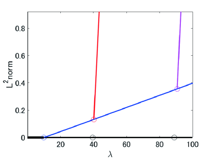
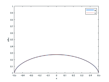
Figure 1. Bifurcation diagram of solutions of (1.2).

Figure 2. Profile of a solution on blue curve at $\lambda=59.8286$.

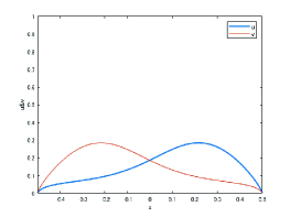
(a) Profile of a solution on red upper branch in Figure 1 at $\lambda=40.3421$.

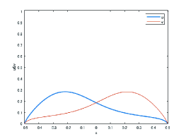
(b) Profile of a solution on red lower branch in Figure 1 at $\lambda=40.3421$.

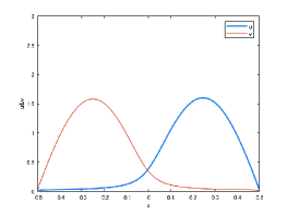
(c) Profile of a solution on red upper branch in Figure 1 at $\lambda=43.0673$.

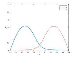
(d) Profile of a solution on red lower branch in Figure 1 at $\lambda=43.0673$.

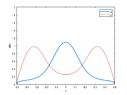
(e) Profile of a solution on purple upper branch in Figure 1 at $\lambda=91.5836$.

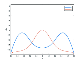
(f) Profile of a solution on purple lower branch in Figure 1 at $\lambda=91.5836$.

Figure 3. Profiles of solutions on red and purple pitchfork bifurcation branches in Figure 1.

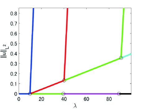
Figure 4. Morse index of solutions of (1.2).

5. Numerical results

In this section, we exhibit the numerical results on the Morse index of positive steady-states by using the continuation software pde2path [4, 7, 33, 34] based on an FEM discretization of the stationary problem. For (1.2), our setting of parameters in the numerical simulation is as follows:

$$\Omega=(-0.5,0.5),\quad\alpha=20,\quad b_{1}=3,\quad b_{2}=2,\quad c_{1}=2,\quad c_{2}=1.$$ (5.1)

Our previous paper with Inoue [10] has already shown the numerical bifurcation diagram as in Figure 1, where the horizontal axis represents the bifurcation parameter $\lambda$, and the vertical axis represents the $L^{2}$ norm of the $u$ component of positive solutions $(u,v)$ to (1.2). In Figure 1, the blue curve is corresponding to the branch $\mathcal{C}_{20,\varLambda}$ of small coexistence (see (1.8)) bifurcating from the trivial solution at $\lambda=\lambda_{1}$. The theoretical value of $\lambda_{1}$ with (5.1) is equal to $\pi^{2}\,(\,\fallingdotseq 9.8696)$. Figure 2, also a reprint from [10], shows the profile of a positive solution $(u,v)$ corresponding to the point at $\lambda=59.8286$ on the blue curve $\mathcal{C}_{20,\varLambda}$. In Figure 1, the red curve exhibits the upper branch $\mathcal{S}_{2,20,\varLambda}^{+}$ and lower one $\mathcal{S}_{2,20,\varLambda}^{-}$ ((1.10) and (1.11)). The pitchfork bifurcation curve $\mathcal{S}_{2,20,\varLambda}$ bifurcates from a solution on the blue curve at $\beta_{2,20}$. It should be noted the $L^{2}$ norm of each component of $\mathcal{S}_{2,20,\varLambda}^{+}$ and $\mathcal{S}_{2,20,\varLambda}^{-}$ are shown overlapped. It was shown in [10] that the secondary bifurcation point $\beta_{2,\alpha}$ theoretically tends to $\lambda_{2}=(2\pi)^{2}\,(\,\fallingdotseq 39.4784)$ as $\alpha\to\infty$. In Figure 3, also a reprint from [10], (a) and (b) exhibit the profiles of solutions on the upper branch $\mathcal{S}^{+}_{2,20,\varLambda}$ and the lower one $\mathcal{S}^{-}_{2,20,\varLambda}$ of the red pitchfork bifurcation curve $\mathcal{S}_{2,20,\varLambda}$ at $\lambda=40.3421$, respectively. It can be observed that $u$ and $v$ are somewhat spatially segregated. Furthermore, as the solution moves away from the bifurcation point on the blue curve, the numerical simulation shows that the segregation between $u$ and $v$ becomes more overt. Actually, (c) and (d) in Figure 3 exhibit the profiles of solutions on $\mathcal{S}^{+}_{2,20,\varLambda}$ and $\mathcal{S}^{+}_{2,20,\varLambda}$ on the red pitchfork bifurcation curve $\mathcal{S}_{2,20,\varLambda}$ at $\lambda=43.0673$, where $u$ and $v$ considerably segregate each other.

The numerical result of this paper is shown in Figure 4 exhibiting the Morse index of each solutions of (1.2) with (5.1). It should be noted that the blue curve in Figure 4 bifurcating from the trivial solution at $\lambda=\lambda_{1}(=\pi^{2}\fallingdotseq 9.8696)$ is corresponding to the bifurcation curve of the semi-trivial solutions $(u,v)=(\theta_{\lambda},0)$ for $\lambda>\lambda_{1}$, which is not included in Figure 1 focusing only on positive solutions. In Figure 4, the blue part is the stable branch of the trivial solution and the semi-trivial solutions; the red part is the unstable branch of the solutions of small coexistence and of segregation with the Morse index $1$; the green part is the unstable branch of the solutions with the Morse index $2$, the light blue part is unstable branch of the solutions with the Morse index $3$.

References

- [1] H. Amann, Dynamic theory of quasilinear parabolic systems, III. Global existence, Math Z., 202 (1989), 219–250.
- [2] H. Amann, Dynamic theory of quasilinear parabolic equations, II. Reaction-diffusion systems, Differ. Int, Eqns., 3 (1990), 13–75.
- [3] H. Amann, Nonhomogeneous linear and quasilinear and parabolic boundary value problems. In: H. Schmeisser, H. Triebel eds. Function Spaces, Differential Operators and Nonlinear Analysis. Teubner-Texte Zur Math., vol. 133, Stuttgart-Leibzig: Teubner, pp. 9–126.
- [4] M. Breden, C. Kuehn, C. Soresina, On the influence of cross-diffusion in pattern formation, J. Comput. Dyn., 8 (2021), 213–240.
- [5] R. S. Cantrell, C. Cosner, Diffusive logistic equations with indefinite weights: population models in disrupted environments, Proc. Royal Soc. Edinburgh A, 112 (1989), 293–318.
- [6] R. S. Cantrell and C. Cosner, Spatial Ecology via Reaction-Diffusion Equations, Wiley Series in Mathematical and Computational Biology. John Wiley & Sons, Ltd., Chichester, 2003.
- [7] T. Dohnal, J. D. M. Rademacher, H. Uecker, D. Wetzel, pde2path 2.0: Multi-parameter continuation and periodic domains, in Proceedings of the 8th European Nonlinear Dynamics Conference, ENOC, 2014 (2014).
- [8] D. Gilbarg, N. S. Trudinger, Elliptic Partial Differential Equations of Second Order, Springer-Verlag, Berlin-Heidelberg, 1998.
- [9] T. Hirose, Y. Yamada, Multiple existence of positive solutions of competing species equations with diffusion and large interactions, Adv. Math. Sci. Appl. Vol. 12 (2002), 435-453.
- [10] J. Inoue, K. Kuto, H. Sato, Coexistence-segregation dichotomy in the full cross-diffusion limit of the stationary SKT model, J. Differ. Equ., 373 (2023), 48–107.
- [11] Y. Kan-on, On the limiting system in the Shigesada, Kawasaki and Teramoto model with large cross-diffusion rates, Discrete Contin. Dyn. Syst. 40 (2020), 3561-3570.
- [12] J.-U. Kim, Smooth solutions to a quasi-linear system of diffusion equations for a certain population model, Nonlinear Anal., 8 (1984), 1121–1144.
- [13] K. Kuto, Limiting structure of shrinking solutions to the stationary SKT model with large cross-diffusion, SIAM J. Math. Anal., 47 (2015), 3993–4024.
- [14] K. Kuto, Full cross-diffusion limit in the stationary Shigesada-Kawasaki-Teramoto model, Ann. Inst. Henri Poincaré C, Anal. Non Linéaire, 38 (2021), 1943–1959.
- [15] K. Kuto, Global structure of steady-states to the full cross-diffusion limit in the Shigesada-Kawasaki-Teramoto model, J. Differ. Equ., 333 (2022), 103–143.
- [16] K. Kuto, Y. Yamada, Positive solutions for Lotka-Volterra competition systems with large cross-diffusion, Appl. Anal., 89 (2010), 1037-1066.
- [17] K. Kuto, Y. Yamada, On limit systems for some population models with cross-diffusion, Discrete Contin. Dyn. Syst. B, 17 (2012), 2745-2769.
- [18] D. Le, Global existence for some cross diffusion systems with equal cross diffusion/reaction rates, Adv. Nonlinear Stud., 20 (2020), 833–845.
- [19] Q. Li, Q. Xu, The stability of nontrivial positive steady states for the SKT model with large cross-diffusion, Acta Math. Appl. Sin. Engl. Ser., 36 (2020), 657–669.
- [20] Q. Li, Y. Wu, Stability analysis on a type of steady state for the SKT competition model with large cross diffusion, J. Math. Anal. Appl., 462 (2018), 1048–1078.
- [21] Q. Li, Y. Wu, Existence and instability of some nontrivial steady states for the SKT competition model with large cross diffusion, Discrete Contin. Dyn. Syst., 40 (2020), 3657–3682.
- [22] Y. Lou, W.-M. Ni, Diffusion, self-diffusion and cross-diffusion, J. Differ. Equ., 131 (1996), 79–131.
- [23] Y. Lou, W.-M. Ni, Diffusion vs cross-diffusion: an elliptic approach, J. Differ. Equ., 154 (1999), 157–190.
- [24] Y. Lou, W.-M, Ni, S. Yotsutani, On a limiting system in the Lotka-Volterra competition with cross-diffusion, Discrete Contin. Dyn. Syst., 10 (2004), 435–458.
- [25] Y. Lou, W.-M, Ni, S. Yotsutani, Pattern formation in a cross-diffusion system, Discrete Contin. Dyn. Syst., 35 (2015), 1589–1607.
- [26] Y. Lou, M. Winkler, Global existence and uniform boundedness of smooth solutions to a cross-diffusion system with equal diffusion rates, Commun. Partial. Differ. Equ., 40 (2015), 1905–1941.
- [27] T. Mori, T. Suzuki, S. Yotsutani, Numerical approach to existence and stability of stationary solutions to a SKT cross-diffusion equation, Math. Models Methods Appl. Sci., 11 (2018), 2191–2210.
- [28] W.-M. Ni, The Mathematics of Diffusion, CBMS-NSF Regional Conference Series in Applied Mathematics 82, SIAM, Philadelphia, 2011.
- [29] W.-M. Ni, Y. Wu, Q. Xu, The existence and stability of nontrivial steady states for S-K-T competition model with cross diffusion, Discrete Contin. Dyn. Syst., 34 (2014), 5271–5298.
- [30] A. Okubo, L. A. Levin, Diffusion and Ecological Problems: Modern Perspective, Second edition. Interdisciplinary Applied Mathematics, 14, Springer-Verlag, New York, 2001.
- [31] W. H. Ruan, Positive steady-state solutions of a competing reaction- diffusion system with large cross-diffusion coefficients, J. Math. Anal. Appl., 197 (1996), 558–578.
- [32] N. Shigesada, K. Kawasaki, E. Teramoto, Spatial segregation of interacting species, J. Theor. Biol., 79 (1979), 83–99.
- [33] H. Uecker, Hopf bifurcation and time periodic orbits with pde2path - algorithms and applications, Commun. Comput. Phys., 25 (2019), 812–852.
- [34] U. Uecker, D. Watzel, J. M. Rademacher, pde2path - A Matlab package for continuation and bifurcation in 2D elliptic systems, Numer. Math. Theory Methods Appl., 7 (2014), 58–106.
- [35] L. Wang, Y. Wu, Q. Xu, Instability of spiky steady states for S-K-T biological competing model with cross-diffusion, Nonlinear Anal., 159 (2017), 424–457.
- [36] Y. Wu, The instability of spiky steady states for a competing species model with cross-diffusion, J. Differ. Equ., 213 (2005), 289–340.
- [37] Y. Wu, Q. Xu, The existence and structure of large spiky steady states for S-K-T competition systems with cross diffusion, Discrete Contin. Dyn. Syst., 29 (2011), 367–385.
- [38] A. Yagi, Abstract Parabolic Evolution Equations and their Applications, Springer-Verlag, Berlin, 2010.
- [39] H. Zhou, Y.-X. Wang, Steady-state problem of an S-K-T competition model with spatially degenerate coefficients, Internat. J. Bifur. Chaos Appl. Sci. Engrg. 31 (11), 2150165 (2021).