Electron Confinement study in a double quantum dot by means of Shannon Entropy Information.

Abstract

In this work, we use the Shannon informational entropies to study an electron confined in a double quantum dot; we mean the entropy in the space of positions, $S_{r}$, in the space of momentum, $S_{p}$, and the total entropy, $S_{t}=S_{r}+S_{p}$. We obtain $S_{r}$, $S_{p}$ and $S_{t}$ as a function of the parameters $A_{2}$ and $k$ which rules the height and the width, respectively, of the internal barrier of the confinement potential. We conjecture that the entropy $S_{r}$ maps the degeneracy of states when we vary $A_{2}$ and also is an indicator of the level of decoupling/coupling of the double quantum dot. We study the quantities $S_{r}$ and $S_{p}$ as measures of delocalization/localization of the probability distribution. Furthermore, we analyze the behaviors of the quantities $S_{p}$ and $S_{t}$ as a function of $A_{2}$ and $k$. Finally, we carried out an energy analysis and, when possible, compared our results with work published in the literature.

Keywords: Shannon Informational Entropies; Double Quantum Dot; Harmonic-Gaussian Symmetric Double Quantum Dot.

1 Introduction

Quantum systems under confinement conditions present notable properties and are studied over a wide range of situations [1, 2]. From the theoretical point of view one finds different approaches and methods to treat these systems, by computing the electronic structure of atoms, ions and molecules under the confinement of a phenomenological external potential in the presence (or not) of external fields. For instance, analytical approximations for two electrons in the presence of an uniform magnetic field under the influence of a harmonic confinement potential representing a single quantum dot (QD) [3, 4, 5], or a quartic one corresponding to a double QD [6]; in this last case the presence of an additional laser field is done through the electron effective mass [7]; or different numerical methods of calculation related to the concern with the accuracy of describing the electron-electron interaction in (artificial) atoms, molecules and nanostructures such as the Hartree approximation [8, 9], the Hartree-Fock computation [10, 11, 12] or the full configuration interaction method (Full CI) [13, 11, 12] among others. Besides, initially the study of confined quantum systems involved the study of the electronic wave function in an atom, or ion, inside a box, whose walls could be partially or not penetrable, and whose description led to the use of different phenomenological potentials [14, 15]. In the case of QD’s, the choice of potential profiles has usually involved a harmonic profile [12, 16, 17, 18], or an exponential one, to take into account the finite size of the confining potential well [19, 20, 21]; or a combination of both [22, 23]. Recently, we have analyzed the behavior of two electrons in a double QD with different confinement profiles, and under the influence of an external magnetic field, aiming at interest in fundamental logical operations of quantum gates [21].

On the other hand, the comprehension of the properties of confined quantum systems is related to the choice of what physical quantities are computed and analysed; in the case of QDs one finds, for instance, the computation of linear and nonlinear absorption coefficients, refractive index, and harmonics generation susceptibilities [24], as well as exchange coupling, electron density function and electronic spatial variance [16, 17]. Although the mathematical basis of information theory was established a long time ago [25, 26, 27], only recently informational entropy has been used as an alternative to the study of the properties of confined quantum systems [28, 29, 30, 31, 32, 33] and in particular QDs [34, 35].

The present work aims to use Shannon informational entropy as a tool to study an electron confined in a double quantum dot. We use a confinement potential composed of a harmonic-gaussian symmetric double quantum well function and harmonic functions. More precisely, by manipulating parameters of the double quantum well function we analyze, for example, the level of decoupling/coupling between neighboring quantum wells. This treatment allows us to study the formation of degenerate and non-degenerate states, as well as the phenomenon of electron tunneling. This approach has applications, among other topics, in quantum computing, where as observed by Loss and DiVincenzo [36] the quantum gate operation of two qubits in a double quantum dot is connected to the decoupling/coupling level between the quantum wells.

Throughout this paper we use atomic units and cartesian coordinate axes. The present paper is organized as follows. In Section 2 our theoretical approach is discussed: in Sec.2.1 the concepts and methodology adopted in this work are presented, in particular the phenomenological confinement potential, whose width, height and coupling are adjusted by different parameters; and in Sec.2.2 the entropy quantities are defined for the sake of completeness. The Sec.3 is also divided in Sec.3.1 and Sec.3.2, where energy and entropies, respectively, are studied as functions of the parameters which rule the potential’s height and coupling.

2 Model and Formulation

This section presents the concepts and methodology of the calculations used in this work. In particular, Subsection 2.1 is dedicated to the presentation of the system formed by an electron confined in a double quantum dot as the physical problem of interest and in Subsection 2.2 the informational quantities $S_{r}$, $S_{p}$ and $S_{t}$ are defined.

2.1 System of interest

2.1.1 Hamiltonian

In the present work we study a system formed by an electron confined in a double quantum dot, whose Hamiltonian is

$$\hat{H}=-\frac{1}{2m_{c}}\vec{\nabla}^{2}+\hat{V}(x,y,z),$$ (1)

where $m_{c}$ is the effective electronic mass and the confinement potential function is given by

$$\hat{V}(x,y,z)=\hat{V}_{DQD}(x)+\hat{V}_{HO}(y)+\hat{V}_{HO}(z)\ .$$ (2)

The potential function $\hat{V}_{DQD}(x)$ is defined by a harmonic-gaussian symmetric double quantum well function, so that,

$$\hat{V}_{DQD}(x)=V_{0}\left[A_{1}\frac{x^{2}}{k^{2}}+A_{2}e^{-\left(\frac{x}{k}\right)^{2}}\right],$$ (3)

with $A_{1}>0$ and $A_{2}>A_{1}$, where $V_{0}$ is the depth of the well and $k$ is the parameter that relates the width of the confinement barrier. The parameters $A_{1}$ adjusts the well to the width of the barrier and $A_{2}$ the height of the internal barrier adjusting the coupling/decoupling between the wells. The potential functions $\hat{V}_{HO}(y)$ and $\hat{V}_{HO}(z)$ are defined by harmonic functions, that is,

$$\hat{V}_{HO}(y) = \frac{1}{2}m_{c}\omega^{2}_{y}y^{2}$$ (4)

and

$$\hat{V}_{HO}(z) = \frac{1}{2}m_{c}\omega^{2}_{z}z^{2}\ ,$$ (5)

where the angular frequencies $\omega_{y}$ and $\omega_{z}$ indicate the confinement parameters.

In the Fig. 1 we present the graph of the confinement potential function, $\hat{V}(x,y,0)$, for A₁ = 0.240, A₂ = 5.000, k = 377.945 a.u., V₀ = 0.00839 a.u., $m_{c}$ = 0.067 a.u. and $\omega_{y}$ = 1.000 a.u. In this figure, we observe the form of the potential function that confines the electron in the double quantum dot, including the infinite barriers of confinement and the internal barrier that regulates the decoupling/coupling between the two wells.

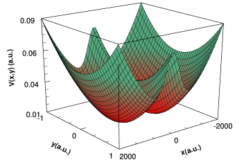
Figure 1: Graph of the confinement potential function $\hat{V}(x,y,0)$ for A₁ = 0.240, A₂ = 5.000, k = 377.945 a.u., V₀ = 0.00839 a.u., $m_{c}$ = 0.067 a.u. and $\omega_{y}$ = 1.000 a.u..

We are interested here in studying the influence of the structure of the double quantum dot on the properties of the system, more precisely, when we vary the parameters $A_{2}$ and $k$ of the potential function $\hat{V}_{DQD}(x)$. Thus, avoid excitation in the directions $\hat{y}$ and $\hat{z}$ and fixed the situation of spatial confinement in these directions determining the potential functions (4) and (5) with $\omega_{y}~{}=1.000$ a.u. and $\omega_{z}~{}=1.000$ a.u..

In Fig. 2 we present graphs with the general behavior of the potential function $\hat{V}_{DQD}(x)$ when: (a) we vary the parameter $A_{2}$ with fixed $k$, $A_{1}$ and $V_{0}$ and (b) we change the values of $k$ with fixed $A_{2}$, $A_{1}$ and $V_{0}$. From graph (a) we see that the increase in $A_{2}$ values increases the level of decoupling between the two wells. Additionally, when the values of $A_{1}$ and $A_{2}$ are very close we have approximately one well in $V_{DQD}(x)$. According to graph (b), the increase in $k$ values increases the width of the confinement barrier. The minimum values of $V_{DQD}(x)$ are changed according to variations in $A_{2}$ or $k$.

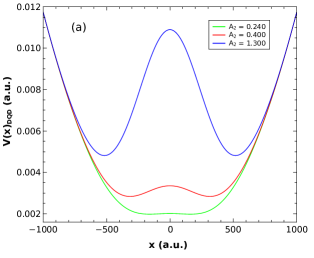
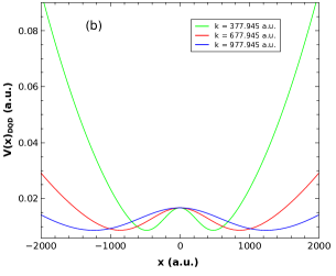
Figure 2: Harmonic-gaussian symmetric double quantum well as a function of $x$ for: (a) different values of $A_{2}$ with $k=$377.945 a.u., $A_{1}=$0.200 and $V_{0}=$0.00838 a.u. and (b) different values of $k$ with $A_{2}=$0.400, $A_{1}=$2.000 and $V_{0}=$0.00838 a.u..

For a deeper understanding of the behavior of the potential function $V_{DQD}(x)$ we present in Fig. S1 of the supplementary material the situations in which we vary the parameter $A_{1}$ with $k$, $A_{2}$ and $V_{0}$ fixed and where we change $V_{0}$ with $A_{1}$, $A_{2}$ and $k$ fixed.

2.1.2 Wave functions and probability densities

Our problem is to solve the Schödinger equation

$$\hat{H}\psi(x,y,z)=E\psi(x,y,z)$$ (6)

adopting the Hamiltonian (1). Here, we write the wave function of an electron

$$\psi(x,y,z)=\psi_{x}(x)\psi_{y}(y)\psi_{z}(z)\$$ (7)

in terms of basis functions of the Cartesian anisotropic Gaussian orbitals (c-aniGTO) type centered at $\vec{R}=(X,0,0)$, that is,

$$\psi_{x}(x) = \sum_{\mu}N_{\mu}C_{\mu}(x-X_{\mu})^{n_{x}}\exp[-\alpha_{\mu}(x-X_{\mu})^{2}].$$ (8)

$$\psi_{y}(y) = N_{y}\ y^{n_{y}}\exp[-\alpha_{y}y^{2}]\ {\rm and}$$ (9)

$$\psi_{z}(z) = N_{z}\ z^{n_{z}}\exp[-\alpha_{z}z^{2}],$$ (10)

where $N_{\mu}$, $N_{y}$ and $N_{z}$ are the normalization constants, $C_{\mu}$ are the molecular orbital coefficients obtained by diagonalization methods and $X_{\mu}$ is defined in $\pm k\sqrt{\ln\left({A_{2}/A_{1}}\right)}$ (minimum values of $\hat{V}_{DQD}(x)$) The integers $n_{x}$, $n_{y}$ and $n_{z}$ allow the classification of orbitals, for example, the types $s-$, $p-$, $d-$, … correspond to $n=n_{x}+n_{y}+n_{z}=$ 0, 1, 2, …., respectively.

In Eq. (8), as we did in previous articles(Refs. [12, 37, 16, 17, 18, 21]), we have considered two types of exponents in $x$, the first Gaussian exponent $\alpha_{x}$ has been obtained variationally, that is, minimizing the functional energy in $x$, and the second proportional to the first as being $\alpha=\frac{3}{2}\alpha_{x}$. In its turn, in Eqs. 9 and 10, $n_{y}$ and $n_{z}$ were taken equal to 0 to avoid excitation in the directions $\widehat{y}$ e $\widehat{z}$. Furthermore, taking $\alpha_{y}=\alpha_{z}=\alpha=\frac{1}{2}m_{c}\omega_{y}$ and $N_{y}=N_{z}=N$, we have

$$\psi_{y}(y) = N\exp[-\alpha(y)^{2}]\ ,$$ (11)

$$\psi_{z}(z) = N\exp[-\alpha(z)^{2}]\ .$$ (12)

The wave function $\widetilde{\psi}(p_{x},p_{y},p_{z})$, in momentum space, has been obtained through a Fourier transform applied to $\psi(x,y,z)$, so that we get

$$\widetilde{\psi}(p_{x},p_{y},p_{z})=\widetilde{\psi_{x}}(p_{x})\widetilde{\psi_{y}}(p_{y})\widetilde{\psi_{z}}(p_{z}),$$ (13)

where

$$\widetilde{\psi_{x}}(p_{x}) = \dfrac{1}{\sqrt{2\pi}}\sum_{\mu}N_{\mu}C_{\mu}e^{-\frac{p_{x}^{2}}{4\alpha_{\mu}}-i{p_{x}X_{\mu}}}\times$$ (14)

$$\sum_{k=0\atop k\text{ even}}^{n_{\mu}}\binom{n_{\mu}}{k}\Big{(}\dfrac{p}{2i\alpha_{\mu}}\Big{)}^{n_{\mu}-k}\dfrac{\Gamma\big{(}\dfrac{k+1}{2}\big{)}}{\alpha_{\mu}^{(k+1)/2}},$$

$$\widetilde{\psi_{y}}(p_{y}) = \dfrac{N}{\sqrt{2\alpha}}\exp\left(-\dfrac{p_{y}^{2}}{4\alpha}\right),{\rm and}$$ (15)

$$\widetilde{\psi_{z}}(p_{z}) = \dfrac{N}{\sqrt{2\alpha}}\exp\left(-\dfrac{p_{z}^{2}}{4\alpha}\right).$$ (16)

The probability density in the position space is defined as usual as

$$\rho(x,y,z) = \rho_{x}(x)\rho_{y}(y)\rho_{z}(z)$$ (17)

$$= |\psi_{x}(x)|^{2}|\psi_{y}(y)|^{2}|\psi_{z}(z)|^{2}\ ,$$

and using the Eqs. (8), (11) and (12), it yields:

$$\rho_{x}(x) = |\psi_{x}(x)|^{2}$$ (18)

$$= \sum_{\mu\nu}N_{\mu}N_{\nu}C_{\mu}^{\ast}C_{\nu}(x-X_{\mu})^{n_{\mu}}(x-X_{\nu})^{n_{\nu}}\times$$

$$\exp\left[-\alpha_{\mu}(x-X_{\mu})^{2}-\alpha_{\nu}(x-X_{\mu})^{2}\right]\ \ ,$$

$$\rho_{y}(y) = |\psi_{y}(y)|^{2}=N^{2}\exp(-2\alpha y^{2})\ ,$$ (19)

$$\rho_{z}(z) = |\psi_{z}(z)|^{2}=N^{2}\exp(-2\alpha z^{2})\ .$$ (20)

Normalizing the densities $\rho_{y}(y)$ and $\rho_{y}(y)$ to unity we find $N^{2}=\sqrt{2\alpha/\pi}$.

The probability density in momentum space is defined as

$$\gamma(p_{x},p_{y},p_{z}) = \gamma_{x}(p_{x})\gamma_{y}(p_{y})\gamma_{z}(p_{z})$$ (21)

$$= |\widetilde{\psi_{x}}(p_{x})|^{2}|\widetilde{\psi_{y}}(p_{y})|^{2}|\widetilde{\psi_{z}}(p_{z})|^{2}$$

where

$$\gamma_{x}(p_{x}) = |\widetilde{\psi_{x}}(p_{x})|^{2}$$ (22)

$$= \dfrac{1}{2\pi}\sum_{\mu\nu}N_{\mu}N_{\nu}C_{\mu}^{\ast}C_{\nu}e^{-\frac{p_{x}^{2}}{4}(1/\alpha_{\mu}+1/\alpha_{\nu})+i{p_{x}(X_{\mu}-X_{\nu})}}\sum_{k=0\atop k\text{ even}}^{n_{\mu}}\sum_{\ell=0\atop\ell\text{ even}}^{n_{\nu}}\binom{n_{\mu}}{k}\binom{n_{\nu}}{\ell}\times$$

$$\Big{(}\dfrac{ip_{x}}{2\alpha_{\mu}}\Big{)}^{n_{\mu}-k}\Big{(}\dfrac{p_{x}}{2i\alpha_{\nu}}\Big{)}^{n_{\nu}-\ell}\dfrac{\Gamma\big{(}\dfrac{k+1}{2}\big{)}}{\alpha_{\mu}^{(k+1)/2}}\dfrac{\Gamma\big{(}\dfrac{\ell+1}{2}\big{)}}{\alpha_{\nu}^{(\ell+1)/2}},$$

$$\gamma_{y}(p_{y}) = |\widetilde{\psi_{y}}(p_{y})|^{2}=\dfrac{1}{\sqrt{2\alpha\pi}}\exp\left(-\dfrac{p_{y}^{2}}{2\alpha}\right),{\rm\ and}$$ (23)

$$\gamma_{z}(p_{z}) = |\widetilde{\psi_{z}}(p_{z})|^{2}=\dfrac{1}{\sqrt{2\alpha\pi}}\exp\left(-\dfrac{p_{z}^{2}}{2\alpha}\right).$$ (24)

We present the details for determining of $\gamma_{x}(p_{x})$ in the supplementary material.

2.2 Shannon informational entropies

In the context of atomic and molecular physics, Shannon informational entropies in the space of positions, $S_{r}$, and momentum, $S_{p}$, can be written as [38, 39]

$$S_{r}=-\int\rho(x,y,z)\ln\left(\rho(x,y,z)\right)d^{3}r$$ (25)

and

$$S_{p}=-\int\gamma(p_{x},p_{y},p_{z})\ln\left(\gamma(p_{x},p_{y},p_{z})\right)d^{3}p.$$ (26)

The probability densities $\rho(x,y,z)$ and $\gamma(p_{x},p_{y},p_{z})$ are defined as in Eqs. (17) e  (21). Adopting $\rho(x,y,z)$ normalized to unity the $S_{r}$ entropy can be written as

$$S_{r} = S_{x}+S_{y}+S_{z}\ ,$$ (27)

where

$$S_{x} = -\int\rho_{x}(x)\ln\left(\rho_{x}(x)\right)dx,$$ (28)

$$S_{y} = -\int\rho_{y}(y)\ln\left(\rho_{y}(y)\right)dy,\textrm{\ and}$$ (29)

$$S_{z} = -\int\rho_{z}(z)\ln\left(\rho_{z}(z)\right)dz.$$ (30)

Analogously, using $\gamma(p_{x},p_{y},p_{z})$ normalized to unity the $S_{p}$ entropy becomes

$$S_{p} = S_{p_{x}}+S_{p_{y}}+S_{p_{z}},$$ (31)

where

$$S_{p_{x}} = -\int\gamma_{x}(p_{x})\ln\left(\gamma_{x}(p_{x})\right)dp_{x}\ ,$$ (32)

$$S_{p_{y}} = -\int\gamma_{y}(p_{y})\ln\left(\gamma_{y}(p_{y})\right)dp_{y},\textrm{\ and}$$ (33)

$$S_{p_{z}} = -\int\gamma_{z}(p_{z})\ln\left(\gamma_{z}(p_{z})\right)dp_{z}.$$ (34)

The quantities $S_{r}$ and $S_{p}$ are interpreted as measures of delocalization or localization of the probability distribution [40, 41].

We determine the entropies $S_{y}$ and $S_{z}$ analytically by replacing Eqs. (19) e (20) in Eqs. (29) and   (30), respectively, so that,

$$S_{y}=S_{z}=-\dfrac{1}{2}\ln\left(\dfrac{2\alpha}{\pi}\right)+\dfrac{1}{2}.$$ (35)

Computing such results in Eq. (27) we have

$$S_{r} = S_{x}-\ln\left(\dfrac{2\alpha}{\pi}\right)+1\ .$$ (36)

$S_{x}$ is calculated numerically using the density (18) in Eq. (28).

Similarly, we obtain the values of $S_{p_{y}}$ and $S_{p_{z}}$ by substituting Eqs. (23) and (24) in Eqs. (33) and  (34), so that

$$S_{p_{y}}=S_{p_{z}}=\frac{1}{2}+\frac{1}{2}\ln(2\pi\alpha).$$ (37)

Considering such results in Eq. (31) one gets

$$S_{p}=S_{p_{x}}+\ln(2\pi\alpha)+1.$$ (38)

$S_{p_{x}}$ is calculated numerically using the density (22) in Eq. (32).

The sum $S_{t}$ is composed of the addition of the quantities $S_{r}$ and $S_{p}$ which, in turn, originate the entropic uncertainty principle mathematized as [42]

$$S_{t} = S_{r}+S_{p}$$ (39)

$$= -\int\rho(x,y,z)\gamma(p_{x},p_{y},p_{z})\ln\left[\rho(x,y,z)\gamma(p_{x},p_{y},p_{z})\right]d^{3}rd^{3}p$$

$$\geq 3(1+\ln\pi).$$

The value of $S_{t}$ is limited by the relation (39) which exhibits a minimum value. From the entropic uncertainty relation we can derive the Kennard uncertainty relation. More specifically, adding the Eqs. (36) e (38) we obtain

$$S_{t}=S_{x}+S_{p_{x}}+2\left[\ln(\pi)+1\right]\geq 3(1+\ln\pi)\ .$$ (40)

Note that this last expression does not depend on $\alpha$.

Shannon entropies are dimensionless quantities from the point of view of physics. However, subtleties surround this issue since, in principle, we have quantities that have physical dimensions in the argument of the logarithmic function. For a more detailed discussion on this topic see Refs. [39, 43, 44].

3 Analysis and Discussion

In this Section, the energy and the entropic quantities $S_{r}$, $S_{p}$ and $S_{t}$ determined by Eqs. (36), (38) and (40) are discussed as a function of the parameter $A_{2}$ and, afterwards, as function of $k$. In the first case we have kept fixed $A_{1}$, $k$ and $V_{0}$; and in the second case, $A_{1}$, $A_{2}$ and $V_{0}$. The specific/fixed values of the parameters in question, besides the values of $m_{c}$ and $V_{0}$ are based in Ref. [22, 23].

The calculations in our study are performed in atomic units (a.u.). In order to compare some of our results with those previously published in the literature we adopt in this section the parameter $k$ in nanometer (nm) and, more specifically, we highlight the energetic contribution along the $x$-axis in meV.

The optimized wave function was expanded into the following basis functions: on the $x$ axis we employ orbitals of the type 2s2p2d2f2g (in total 10 functions located in each well) and on the $y$ and $z$ axes, 1s type orbitals. In cases where states are degenerate, symmetrization and antisymmetrization were done.

3.1 Energy analysis

We present in Fig. 3 the energy curves $E_{n}$ (contribution along the $x$-axis) as a function of the parameter $A_{2}$ ranging from 0.240 to 5.000 for the first six quantum states $(n=0-5)$ with $A_{1}$ = 0.200, k = 20.000 nm and V₀ = 228.00 meV. Inset: it is detailed the energy curves for the $A_{2}$ ranging from 0.240 to 1.050, where states initially non-degenerate become degenerate two by two as $A_{2}$ increases. In Table S1 of the supplementary material you can find the energy values as a function of $A_{2}$.

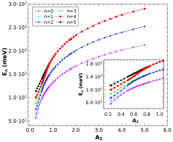
Figure 3: Energy contribution along the $x$-axis for states $n=0-5$ as a function of $A_{2}$, for $A_{1}=$ 0.200, $k=$ 20.000 nm and V${}_{0}=$ 228.00 meV. The inset details the region where the states are completely non-degenerate and merge two by two into one.

According to the Table S1, we have that the degeneracy for states $n$ = 0 and $n$ = 1 appears in the interval of $1.200\leq A_{2}\leq 1.400$, and at $A_{2}$ = 1.300 we have $E_{0}=E_{1}=$ 146.24146 meV. The degeneracies in $n$ = 2 and $n$ = 3 originate at values of $1.400\leq A_{2}\leq 1.600$, and at $A_{2}$ = 1.500 we find $E_{2}$ = $E_{3}$ = 184.54417 meV. Finally, the degeneracies in $n=4$ and $n$ = 5 begin between $1.800\leq A_{2}\leq 2.000$, and at $A_{2}$ = 1.900 we have $E_{4}$ = $E_{5}$ = 230.14020 meV. Otherwise, we observe by inset of Fig. 3 that the decrease in the values of $A_{2}$ causes the system to rely on non-degenerate states.

In Fig. 4a we present the probability density curves in the position, $\rho_{x}(x)$ , as a function of $x$ for the ground state and different values of $A_{2}$. In the curves of $\rho_{x}(x)$ for $A_{2}$ = 0.240 and 0.400 the state is not degenerate, in this case, the electron has the probability of being in one or both wells of the function $V_{DQD}(x)$, and even above the internal barrier. In the curves of $\rho_{x}(x)$ for $A_{2}$ = 1.300 and 1.400 the state is degenerate and the electron has the probability of being in only one of the wells of $V_{DQD}(x)$. For completeness, in Fig. 4b we present the probability density curves in the momentum, $\gamma_{x}(p_{x})$, as a function of $p$ for the ground state for $A_{2}$ = 0.240, 0.400, 1.300 and 1.400.

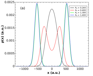
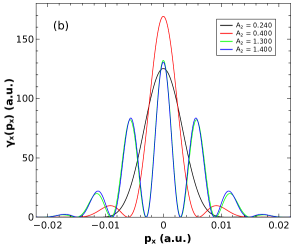
Figure 4: Probability densities $\rho_{x}(x)$ and $\gamma_{x}(p_{x})$ in the position and momentum space, respectively, for the ground state with different values of $A_{2}$, for $A_{1}$ = 0.200, $k$ = 20.000 nm and V${}_{0}=$ 228.00 meV.

In the main graph of Fig. 5 we present the energy curves $E_{n}$ (contribution along the $x$-axis) for the first six quantum states $(n=0-5)$ as a function of the parameter $k$ varying from 0.500 nm to 30.000 nm with $A_{1}$ = 0.400, $A_{2}$ = 2.000 and V₀ = 228.00 meV. Furthermore, we indicate in the insets (a) the energy curves with the parameter $k$ varying from 0.500 nm to 3.500 nm and (b) the energy curves with $k$ varying from 11.000 nm to 30.000 nm. In Table S2 of the supplementary material the values obtained for energies as a function of $k$ can be found.

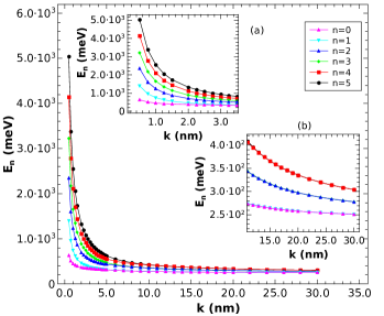
Figure 5: Energy contribution along the $x$-axis for states $n$ = 0-5 as a function of $k$, for $A_{1}$ = 0.400, $A_{2}$ = 2.000 and V₀ = 228.00 meV. The insets show the non-degenerate region of the energy curves (0.5 $\leq$ k $\leq$ 3.5 nm) and the degenerate one (11.0 $\leq$ k $\leq$ 30.0 nm).

We observe in the main graph of Fig. 5 and inset (b) that with the increase in the values of $k$ the energies merge two by two into one, that is, $E_{0}=E_{1}$, $E_{2}=E_{3}$, $E_{4}=E_{5}$. By inset (a), with the decrease in the values of $k$ and the increase in the effects of confinement, we identify the appearance of non-degenerate states, besides, we have on considerable increase in the values of $E_{n}$.

In the graphs of Fig. 6 we present the probability density curves for the ground state in the position and momentum space, $\rho_{x}(x)$ (Fig.  6a) and $\gamma_{x}(p_{x})$ (Fig. 6b), respectively, for different values of $k$. In both cases, $\rho_{x}(x)$ and $\gamma_{x}(p_{x})$, for the value of $k$ = 0.500 nm the ground state is non-degenerate, otherwise, for $k$ = 17.000 nm, 19.000 nm and 30.000 nm the state is degenerate. In this way, we perceive changes in the shape of the probability distributions when the values of $k$ imply or not degeneracy in energies.

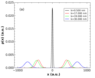
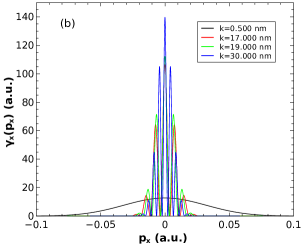
Figure 6: Probability densities $\rho_{x}(x)$ and $\gamma_{x}(p_{x})$ in the position and momentum space, respectively, for the ground state with different values of $k$, for $A_{1}$ = 0.400, $A_{2}$ = 2.000 and V₀ = 228.00 meV.

As long as comparison has been possible, we have obtained a good agreement with the values found in Ref. [22, 23] regarding the energy as a function of $A_{2}$ and $k$. As in the present work, Duque et al have also used matrix diagonalization methods; however, they have adopted an expanded wave function in terms of orthonormal trigonometric functions.

3.2 Informational Analysis

In the main graph of Fig. 7 we present the curves of Shannon entropy in the space of positions for the first six quantum states $(n=0-5)$, $S^{n}_{r}$, as a function of the parameter $A_{2}$ ranging from 0.240 to 5.000 with $A_{1}$ = 0.200, $k$ = 20.000 nm and V₀ =228.00 meV. The inset details the curves of $S^{n}_{r}$ in the range of $A_{2}=$0.240 to 1.100. In Table S3 of the supplementary material we provide the values of $S^{n}_{r}$ as a function of $A_{2}$.

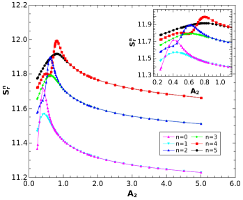
Figure 7: Shannon entropy, $S^{n}_{r}$, for states $n=0-5$ as a function of $A_{2}$ ranging from 0.240 to 5.000, for $A_{1}$ = 0.200, $k$ = 20.000 nm and V₀ =228.00 meV. In the inset, it is detailed the initial behaviour of $S^{n}_{r}$ as a function of $A_{2}$.

According to Fig. 7 we notice that the values of the Shannon entropy curves $S^{n}_{r}$ get closer two by two as $A_{2}$ increases, i.e., $S^{0}_{r}\rightarrow S^{1}_{r}$, $S^{2}_{r}\rightarrow S^{3}_{r}$ and $S^{4}_{r}\rightarrow S^{5}_{r}$. In Table S3, we identified that the degeneracy of $S^{n}_{r}$ for states $n=0$ and $n=1$ appears in the values of $A_{2}$ comprised between $1.300\leq A_{2}\leq 1.500$, and at $A_{2}=$ 1.400 we have $S^{0}_{r}=S^{1}_{r}=$ 11.35961. The degeneracy in $S^{n}_{r}$ for states $n=2$ and $n=3$ becomes evident in the interval $1.400\leq A_{2}\leq 1.600$, and at $A_{2}=$ 1.500 we find $S^{2}_{r}=S^{3}_{r}=$ 11.63816. Finally, although at $A_{2}=$ 1.750 we already have $S^{4}_{r}=S^{5}_{r}=$ 11.78527, the degeneracy in $S^{n}_{r}$ for $n=4$ and $n=5$ appears in the values between $1.800\leq A_{2}\leq 2.000$, and at $A_{2}=$ 1.900 we have the identical value of $S^{4}_{r}=S^{5}_{r}=$ 11.77304.

In Table 1 we present the regions of $A_{2}$ where the degeneracies in energy and entropy $S^{n}_{r}$ for states $n=0-5$ originate. For states $n=0$ and $n=1$, the range of values of $A_{2}$ where this occurs coincides reasonably with the range of values of $A_{2}$ where the degeneracy in $S^{n}_{r}$ originates. For states $n=2$ and $n=3$, and also for $n=4$ and $n=5$, the set of values of $A_{2}$, where the degeneracy in energies and in $S_{r}$ originate, are identical. In this way, we conjecture that the Shannon entropy in the space of positions, $S^{n}_{r}$, can successfully map the degeneracy of states when we vary the values of $A_{2}$ in the double quantum dot studied.

Table 1: Range of $A_{2}$ where degeneracies in energies and entropy $S^{n}_{r}$ for states $n=0-5$ originate.

	Range of $A_{2}$
States	Energy	$S_{r}$
n=0 e n=1	1.200 < $A_{2}$ <1.400	1.300 < $A_{2}$ <1.500
n=2 e n=3	1.400 < $A_{2}$ <1.600	1.400 < $A_{2}$ <1.600
n=4 e n=5	1.800 < $A_{2}$ <2.000	1.800 < $A_{2}$ <2.000

By analyzing the inset of Fig. 7 we see that as $A_{2}$ decreases, the values of $S^{n}_{r}$ increase until they reach a maximum value and, from that point on, they decrease again. The oscillations for the values of $S^{n}_{r}$ can be justified taking into account that the information entropies reflect a measure of the delocalization/localization of $\rho_{x}(x)$. For example, for the ground state, according to Table S3, we highlight that: at $A_{2}=1.300$ we have $S^{0}_{r}=$ 11.37033, at $A_{2}=$ 0.400 we have a maximum value of $S^{0}_{r}=$ 11.71876 and, finally, at $A_{2}=$ 0.240 we find $S^{0}_{r}=$ 11.36528. These values of $S^{n}_{r}$ agree with Fig. 4(a), since the delocalization of the green curve is smaller than that of the red curve which, in turn, is greater than that of the black curve. Similar analyzes can be undertaken for other states.

Taking the state $n=0$ in Fig. 7, starting from $A_{2}=0.240$, where $S^{0}_{r}=11.36528$, the values of $S^{0}_{r}$ increase up to the maximum value of $S^{0}_{r}=11.71876$ in $A_{2}=0.400$. From this point of maximum entropy, the values of $S^{0}_{r}$ decrease, passing through $A_{2}=1.300$ where $S_{r}=11.37033$. We observe in Fig. 2(a) that it is precisely at $A_{2}=0.400$ that the internal barrier of $V_{DQD}(x)$ begins to influence the decoupling between the two wells. Still, from Fig. 2(a), in $A_{2}=1.300$ the internal barrier of the function $V_{DQD}(x)$ is quite consolidated, strongly favoring the decoupling between the two wells of the function. In this way, we conjecture that the information entropy by means of $S^{0}_{r}$ is an indicator of the level of decoupling/coupling of the double quantum dot studied.

In the graph in Fig. 8 we present for the first six quantum states $(n=0-5)$ the Shannon entropy curves in the space of positions, $S^{n}_{r}$, as a function of the parameter $k$ varying from 0.500 nm to 30.000 nm with $A_{1}=0.400$, $A_{2}=2.000$ and $V_{0}=228.00$ meV. In the inset we highlight $S^{n}_{r}$ in the range from $k=0.500$ nm to 5.000 nm. In Table S4 of the supplementary material we provide the values of $S^{n}_{r}$ as a function of $k$.

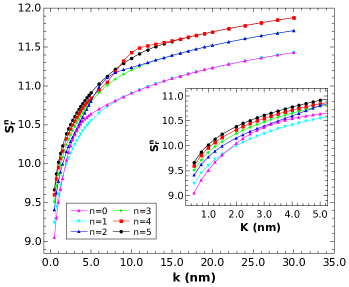
Figure 8: Shannon entropy, $S^{n}_{r}$, for states $n=0-5$ as a function of $k$ ranging from 0.500 to 30.000 nm, for $A_{1}$ = 0.400, $A_{2}$ = 2.000 and $V_{0}=228.00$ meV. In the inset, $S^{n}_{r}$ as a function of $k$ ranging from 0.500 to 5.000 nm.

According to the main graph of the Fig. 8 when $k$ tends to infinity degeneracy arises in the values of $S_{r}$ such that $S^{0}_{r}=S^{1}_{r}$, $S^{2}_{r}=S^{3}_{r}$ and $S^{4}_{r}=S^{5}_{r}$. An increase in the values of $k$ widens the barriers of the potential function $V_{DQD}(x)$ reducing the effects of confinement. In this situation, the uncertainty in determining the location of the electron increases and, consequently, we identify an increase in the values of $S^{n}_{r}$. In fact, as $k$ increases the delocalization in $\rho_{x}(x)$ increases according to Fig. 6 (a).

On the other hand, we observe in the inset of Fig. 8 that as $k$ decreases there is a break in the degeneracy of $S^{n}_{r}$. Furthermore, the decrease in $k$ generates a narrowing in the barriers of the potential function $V_{DQD}(x)$. In this case, there is an increase in the confinement situation and, consequently, a decrease in uncertainty in the location of the electron, causing $S^{n}_{r}$ values to decrease. Here, the delocalization in $\rho_{x}(x)$ decreases according to Fig. 6(a).

In Fig. 9 we display for the first six quantum states ($n=0-5$) the Shannon entropy curves in the momentum space, $S^{n}_{p}$, as a function of the parameter $A_{2}$ varying from 0.240 to 5.000 with $A_{1}$ = 0.200, $k$ = 20.000 nm and V₀ = 228.00 meV. In Table S5 of the supplementary material we provide the values of $S^{n}_{p}$ as a function of $A_{2}$.

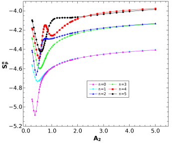
Figure 9: Shannon entropy, $S^{n}_{p}$, for states $n=0-5$ as a function of $A_{2}$ ranging from 0.240 to 5.000, for $A_{1}$ = 0.200, $k$ = 20.000 nm and V₀ = 228.00 meV.

We have from Fig. 9 and according to Table S5 that when $A_{2}$ increases occurs that $S^{0}_{p}\rightarrow S^{1}_{p}$. We did not identify degeneration in $S^{2-5}_{p}$. In general, with the decrease in $A_{2}$ the values of $S^{n}_{p}$ also decrease until they reach a minimum value, then increase again. Similar to what we did for $S^{n}_{r}$ the oscillatory behavior of the values of $S^{n}_{p}$ can be explained based in the curves of $\gamma_{x}(p_{x})$ in the Fig. 4.

In Fig. 10 we present for the first six quantum states $(n=0-5)$ the Shannon entropy curves in momentum space, $S^{n}_{p}$, as a function of the parameter $k$ varying from 0.500  nm up to 30.000 nm with $A_{1}$ = 0.400, $A_{2}$ = 2.000 and $V_{0}$ = 228.00 meV. In Table S6 of the supplementary material we have the values of $S^{n}_{p}$ as a function of $k$.

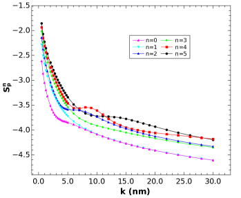
Figure 10: Shannon entropy, $S^{n}_{p}$, for states $n=0-5$ as a function of $k$ ranging from 0.500 to 30.000 nm, for $A_{1}$ = 0.400, $A_{2}$ = 2.000 and $V_{0}$ = 228.00 meV.

According to the Fig. 10 and Table S6 when the values of $k$ increase we have degeneracy in $S^{0}_{p}$ and $S^{1}_{p}$. We did not identify degeneration in $S^{2-5}_{p}$. On the other hand, when $k$ decrease the values of $S^{n}_{p}$ increases. The behavior of the curve for $n$ = 4 shows intriguing oscillations.

All values of $S^{n}_{p}$ obtained in this work are negative as can be seen in Tables S5 e S6 of the supplementary material. This result has an explanation in the quantum context [45], that is, when the limits of confinement are very small, the probability density becomes large and $\rho(x,y,z)>1$. In this situation, $-\rho(x,y,z)\ln(\rho(x,y,z))<0$ and so $S_{p}$ (or $S_{r}$) can be negative. The original work by Shannon [27] also indicates the possibility of obtaining negative values for informational entropy when working with continuous distributions.

In Fig. 11 we present for the first six quantum states $(n=0-5)$ the entropy sum curves $S^{n}_{t}$ as a function of the parameter $A_{2}$ varying from 0.240 to 5.000 with $A_{1}$ = 0.200, $k$ = 20.000 nm and V₀ = 228.00 meV . In Table S7 of the supplementary material we provide the values of $S^{n}_{t}$ as a function of $A_{2}$.

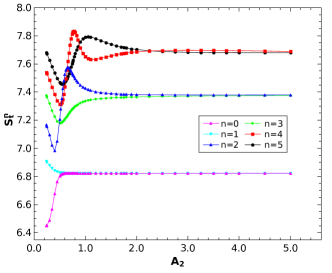
Figure 11: Entropy sum, $S^{n}_{t}$, for states $n=0-5$ as a function of $A_{2}$ ranging from 0.240 to 5.000, for $A_{1}$ = 0.200, $k$ = 20.000 nm and V₀ = 228.00 meV.

From Fig. 11 and Table S7, as $A_{2}$ increases we have $S^{0}_{t}\rightarrow S^{1}_{t}$. We did not identify degeneracy in $S^{2-5}_{t}$. Furthermore, when $A_{2}$ tends to infinity $S^{n}_{t}$ tends to constant values. More specifically, the values of $S^{0}_{t}=6.44814$ for $A_{2}=0.240$ and $A_{1}=0.200$ (see green curve in Fig. 2a) is a value approximately equal to three times the value of the entropy sum for the one-dimensional harmonic oscillator in the ground state presented in Ref. [43].

We identify in Fig. 11 oscillations in the $S^{n}_{t}$ curves with the occurrence of maximum and minimum values for states $n=2-5$. An elegant explanation for the extreme values of the entropy sum is presented in Ref. [34], that is, in general, the derivative of $S_{t}$ with respect to $A_{2}$ is given by $\frac{\partial S_{t}}{\partial A_{2}}=\frac{\partial S_{r}}{\partial A_{2}}+\frac{\partial S_{p}}{\partial A_{2}}$. Since the extreme points in the curves occur when $\frac{\partial S_{t}}{\partial A_{2}}=0$ with the absolute values $|\frac{\partial S_{r}}{\partial A_{2}}|$ and $|\frac{\partial S_{p}}{\partial A_{2}}|$ being equal.

The Fig. 12 displays for the first six quantum states $(n=0-5)$ the entropy sum curves $S^{n}_{t}$ as a function of the parameter $k$ ranging from 0.500 nm to 30.000 nm with $A_{1}$ = 0.400, $A_{2}$ = 2.000 and $V_{0}$ = 228.00 meV. In Table S8 of the supplementary material we provide the values of $S^{n}_{t}$ as a function of $k$.

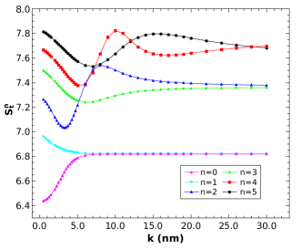
Figure 12: Entropy sum, $S^{n}_{t}$, for states $n=0-5$ as a function of $k$ ranging from 0.500 to 30.000 nm, for $A_{1}$ = 0.400, $A_{2}$ = 2.000 and $V_{0}$ = 228.00 meV.

As shown in Fig. 12 as $k$ grows, we see a degeneracy of $S^{0}_{t}$ and $S^{1}_{t}$. For $S^{2-5}_{t}$ we did not identify degeneration. When $k$ tends to infinity, the values of $S^{n}_{t}$ tend to constant values. With the decrease in the values of $k$, oscillations appear in the curves of $S^{2-5}_{t}$, such oscillations can be analyzed in a similar way as we presented previously, that is, taking into account the derivative of $S_{t}$ in relation to $k$.

The values of $S_{r}$ and $S_{p}$, whether as a function of $A_{2}$ or $k$, are compatible with the entropic uncertainty relationship. Furthermore, all values of $S_{t}$ obtained in this work (see Tables S7  and S8) are above the minimum value of 6.43419 that the entropy sum can assume according to the Eq. (40).

4 Conclusion

We have studied the electronic confinement in a double quantum dot using Shannon informational entropies. The confinement potential $\hat{V}(x,y,z)$ has been described phenomenologically by using a 3D harmonic-gaussian function representing a double quantum dot symmetric in the $x$ direction, and with a harmonic profile in the $y$ and $z$ directions. In particular, we have varied the parameters $A_{2}$ and $k$, which are related to the height and the width of the confinement potential internal barrier, respectively.

We have initially established the energetic contribution along the $x$ direction for the first six quantum states of the system (n=0-5). We have analyzed the values of the parameter $A_{2}$ for which the energy values correspond to the degenerate and non-degenerate states. Regarding the $k$ parameter, we have highlighted the considerable increase in energy values when the values of this quantity tend to zero, increasing the confinement effects on the electron. As long as comparison was possible, we have obtained a good agreement with the values of energy as a function of $A_{2}$ and $k$ found in the literature.

We have obtained the entropy values $S^{n}_{r}$ as a function of $A_{2}$ and $k$ for the quantum states $n=0-5$. In the first situation, we conjecture that the entropy $S^{n}_{r}$ successfully maps the degeneration of states when we vary the coupling parameter $A_{2}$. We also conclude that information entropy, through $S^{0}_{r}$, is an indicator of the level of decoupling/coupling of the double quantum dot. Furthermore, taking into account that informational entropies are used as a measure of delocalization/localization of $\rho_{x}(x)$, we justify the fluctuations in the values of $S^{n}_{r}$ as a function of $A_{2}$ and present the study of the values of $S^{n}_{r}$ as a function of $k$.

In addition to the informational analysis, we have determined the values of $S^{n}_{p}$ and $S^{n}_{t}$ as functions of $A_{2}$ and $k$. In this treatment, analyzing trends and, through the derivative of $S^{n}_{t}$, we focus on general aspects of the behavior of the values obtained. Additionally, we conclude that all values obtained for $S^{n}_{t}$ respect the entropic uncertainty relationship. In future work we shall delve deeper into the physical explanations about the behavior of the values of $S^{n}_{p}$ and $S^{n}_{t}$ as a function of $A_{2}$ and $k$.

Finally, from another perspective of work, we shall also use Shannon’s informational entropies to analyze an electron confined in a double quantum dot, however, this time subjected to external fields.

Supporting Information

This manuscript contains supplementary information. Click here to access.

Acknowledgements

The authors acknowledge Conselho Nacional de Desenvolvimento Científico e Tecnológico (CNPq) and Coordenação de Aperfeiçoamento Pessoal de Nível Superior (CAPES) for the financial support.

Conflict of Interest

The authors declare no conflict of interest.

References

- [1] Sabin J R and Brandas E J (eds) 2009 Advances in quantum chemistry: theory of confined quantum systems-part one vol 57 and 58 (Academic Press) https://www.elsevier.com/books/advances-in-quantum-chemistry/sabin/978-0-12-374764-8 and https://www.elsevier.com/books/advances-in-quantum-chemistry/sabin/978-0-12-375074-7
- [2] Sen K D (ed) 2014 Electronic structure of quantum confined atoms and molecules (Springer) URL https://doi.org/10.1007/978-3-319-09982-8
- [3] Merkt U, Huser J and Wagner M 1991 Phys. Rev. B 43 7320 URL https://doi.org/10.1103/PhysRevB.43.7320
- [4] Wagner M, Merkt U and Chaplik A 1992 Phys. Rev. B 45 1951 URL https://doi.org/10.1103/PhysRevB.45.1951
- [5] Quiroga L, Ardila D and Johnson N 1993 Solid State Commun. 86 775–780 URL https://doi.org/10.1016/0038-1098(93)90107-X
- [6] Burkard G, Loss D and DiVincenzo D P 1999 Phys. Rev. B 59(3) 2070–2078 URL https://link.aps.org/doi/10.1103/PhysRevB.59.2070
- [7] Carvalho C R, Jalbert G, Rocha A B and Brandi H S 2003 J. Appl. Phys. 94 2579–2584 URL https://doi.org/10.1063/1.1591058
- [8] Pfannkuche D, Gudmundsson V and Maksym P A 1993 Phys. Rev. B 47 2244 URL https://doi.org/10.1103/PhysRevB.47.2244
- [9] Creffield C E, Jefferson J H, Sarkar S and Tipton D 2000 Phys. Rev. B 62 7249 URL https://doi.org/10.1103/PhysRevB.62.7249
- [10] Szafran B, Bednarek S, Adamowski J, Tavernier M, Anisimovas E and Peeters F 2004 Eur. Phys. J. D 28 373–380 URL https://doi.org/10.1140/epjd/e2003-00320-5
- [11] Thompson D C and Alavi A 2005 J. Chem. Phys. 122 URL https://doi.org/10.1063/1.1869978
- [12] Olavo L S F, Maniero A M, de Carvalho C R, Prudente F V and Jalbert G 2016 J. Phys. B: At. Mol. Opt. Phys. 49 145004 URL https://doi.org/10.1088/0953-4075/49/14/145004
- [13] Jung J and Alvarellos J 2003 J. Chem. Phys. 118 10825–10834 URL https://doi.org/10.1063/1.1574786
- [14] Fröman P O, Yngve S and Fröman N 1987 J. Math. Phys. 28 1813–1826 URL https://doi.org/10.1063/1.527441
- [15] Connerade J P and Semaoune R 2000 J. Phys. B: At. Mol. Opt. Phys. 33 3467 URL https://dx.doi.org/10.1088/0953-4075/33/17/323
- [16] Maniero A M, de Carvalho C R, Prudente F V and Jalbert G 2020 J. Phys. B: At. Mol. Opt. Phys. 53 185001 URL https://doi.org/10.1088/1361-6455/ab9f0f
- [17] Maniero A M, de Carvalho C R, Prudente F V and Jalbert G 2020 arXiv preprint arXiv:2004.09459 URL https://arxiv.org/abs/2004.09459
- [18] Maniero A M, de Carvalho C R, Prudente F V and Jalbert G 2021 J. Phys. B: At. Mol. Opt. Phys. 54 11LT01 URL https://doi.org/10.1088/1361-6455/abf2dc
- [19] Adamowski J, Sobkowicz M, Szafran B and Bednarek S 2000 Phys. Rev. B 62(7) 4234–4237 URL https://link.aps.org/doi/10.1103/PhysRevB.62.4234
- [20] Xie W 2003 Solid State Commun. 127 401–405 ISSN 0038-1098 URL https://www.sciencedirect.com/science/article/pii/S0038109803003351
- [21] Maniero A M, Prudente F V, de Carvalho C R and Jalbert G 2023 Phys. B (Amsterdam, Neth.) 657 414818 ISSN 0921-4526 URL https://www.sciencedirect.com/science/article/pii/S0921452623001850
- [22] Kasapoglu E, Yücel M B and Duque C A 2023 Nanomaterials 13 ISSN 2079-4991 URL https://www.mdpi.com/2079-4991/13/5/892
- [23] Kasapoglu E, Yücel M B and Duque C A 2023 Nanomaterials 13 ISSN 2079-4991 URL https://www.mdpi.com/2079-4991/13/8/1360
- [24] TA Sargsian PA Mantashyan D H 2023 Nano-Structures and Nano-Objects 33 100936 URL https://doi.org/10.1016/j.nanoso.2022.100936
- [25] Nyquist H 1928 Trans. A.I.E.E. 47 617–644 URL https://doi.org/10.1109/T-AIEE.1928.5055024
- [26] Hartley R V L 1928 Bell Syst. Tech. Journal 7 535–563 URL https://doi.org/10.1002/j.1538-7305.1928.tb01236.x
- [27] Shannon C E 1948 Bell Syst. Tech. Journal 27 379–423 URL https://doi.org/10.1002/j.1538-7305.1948.tb01338.x
- [28] Mukherjee N and Roy A K 2016 Ann. Phys. (Berlin) 528 412–433 URL https://onlinelibrary.wiley.com/doi/abs/10.1002/andp.201500301
- [29] Nascimento W S, de Almeida M M and Prudente F V 2021 Eur. Phys. J. D 75 171 URL https://doi.org/10.1140/epjd/s10053-021-00177-6
- [30] Estañón C R, Aquino N, Puertas-Centeno D and Dehesa J S 2020 Int. J. Quantum Chem. 120 e26192 URL https://onlinelibrary.wiley.com/doi/abs/10.1002/qua.26192
- [31] Saha S and Jose J 2020 Int. J. Quantum Chem. 120 e26374 URL https://onlinelibrary.wiley.com/doi/abs/10.1002/qua.26374
- [32] Salazar S J C, Laguna H G, Dahiya B, Prasad V and Sagar R P 2021 Eur. Phys. J. D 75 127 URL https://doi.org/10.1140/epjd/s10053-021-00143-2
- [33] Santos A d J, Prudente F V, Guimarães M N and Nascimento W S 2022 Quantum Rep. 4 544–557 URL https://doi.org/10.3390/quantum4040039
- [34] Liu X, Xie X y, Wang D h, Wang C l, Zhao Y l and Zhang S f 2023 Philos. Mag. 103 892–913 URL https://doi.org/10.1080/14786435.2023.2173818
- [35] Mondal S, Sen K and Saha J K 2022 Phys. Rev. A 105(3) 032821 URL https://link.aps.org/doi/10.1103/PhysRevA.105.032821
- [36] Loss D and DiVincenzo D P 1998 Phys. Rev. A 57 120–126 URL https://doi.org/10.1103/PhysRevA.57.120
- [37] Maniero A M, de Carvalho C R, Prudente F V and Jalbert G 2019 J. Phys. B: At. Mol. Opt. Phys. 52 095103 URL https://doi.org/10.1088/1361-6455/ab0574
- [38] Sen K D (ed) 2011 Statistical Complexity: Applications in Electronic Struture (Dordrecht: Springer) URL https://doi.org/10.1007/978-90-481-3890-6
- [39] Nascimento W S and Prudente F V 2018 Chem. Phys. Lett. 691 401 URL https://www.sciencedirect.com/science/article/pii/S0009261417310655
- [40] Corzo H H, Laguna H G and Sagar R P 2012 J. Math. Chem. 50 233 URL https://doi.org/10.1007/s10910-011-9908-2
- [41] Cruz E, Aquino N and Prasad V 2021 Eur. Phys. J. D 75 106 URL https://doi.org/10.1140/epjd/s10053-021-00119-2
- [42] Bialynicki-Birula I and Mycielski J 1975 Commun. Math. Phys. 44 129 URL https://doi.org/10.1007/BF01608825
- [43] Nascimento W S, de Almeida M M and Prudente F V 2020 Eur. J. Phys. 41 025405 URL https://dx.doi.org/10.1088/1361-6404/ab5f7d
- [44] Matta C F, Sichinga M and Ayers P W 2011 Chem. Phys. Lett. 514 379–383 ISSN 0009-2614 URL https://www.sciencedirect.com/science/article/pii/S0009261411010530
- [45] Aquino N, Flores-Riveros A and Rivas-Silva J 2013 Phys. Lett. A 377 2062 URL https://www.sciencedirect.com/science/article/abs/pii/S0375960113005367