Dynamical simulations of colliding superconducting strings

Abstract

We study the collisions of elastic superconducting strings, also referred to as current-carrying strings, formed in a $U_{\rm local}(1)\times U_{\rm global}(1)$ field-theory model, using three-dimensional numerical field-theoretic simulations. The breaking of $U_{\rm local}(1)$ leads to string formation via the Higgs mechanism, while the scalar field of the second $U_{\rm global}(1)$ carries the current, which condenses onto the string. We construct straight and static superconducting string solutions numerically and identify the regions in which they exist in the model parameter space. We then perform dynamical simulations for colliding superconducting strings with various collision angles and collision velocities. We explore the kinematic parameter space for six sets of model parameters characterising the coupling between the two scalar fields and the current on the string. The final states of the strings (after the collision) are reported diagrammatically. We classify them into four categories: (i) regular intercommutation, (ii) double intercommutation, (iii) bound state, and (iv) expanding string solution. We find that the outcome of the collision process is the regular intercommutation of the colliding strings in most of the kinematic parameter space while they form bound states for small velocities and small angles. We also find that the strings undergo two successive intercommutations and therefore pass through one other in a small region corresponding to relatively small angles and velocities of order $c/2$. The string structure breaks down when there is a relatively large coupling between the two scalar fields even if each string is stable before the occurrence of the collision.

I Introduction

Cosmic strings can form in many models of grand-unification, see, e.g., [1], and hence, determining their observational consequences — be it via gravitational waves, lensing, cosmic microwave background physics, or any other means — is of great interest [2, 3, 4, 5]. Indeed, if any signature of cosmic strings was to be observed (so far, only bounds exist), it would provide invaluable information about the Universe during its phase transitions, and open up a window on fundamental physics at very high energies, such as axion physics [6, 7, 8, 9, 10, 11, 12, 13, 14], grand-unification [15, 1, 16, 17] and the seesaw mechanism [18, 19, 20].

Central to any calculation of the observational consequences of cosmic strings is that the string network reaches a “scaling solution”, in which the energy density in the strings is a small fixed fraction of the energy density in the Universe. Most of the work related to string networks has been based on the Abelian-Higgs model for cosmic strings; in this particular case, strings generally intercommute when colliding (see below). This crucial fact means that the string network will form closed loops during its evolution; these loops radiate energy in the form of gravitational waves (see, e.g., [21, 22, 23, 24, 25, 26, 27, 28, 29, 30, 31, 32, 33, 34, 35, 36, 37, 22, 38, 39, 21, 40, 41, 42, 43, 44, 45, 46, 47, 48, 49, 50, 51, 52, 53, 54, 55, 56, 57, 58]), and it is for this reason that the network evolves towards an attractor scaling solution (see, e.g., [59, 60, 61, 62, 63, 64, 65, 66]). In this regime, there is a unique length scale, called the correlation length. The (velocity-dependent) one-scale model was developed with this particular property in mind [59, 67, 68, 69, 61, 62, 70], and allows one to estimate the present power spectrum of the gravitational waves generated by cosmic strings as well as the contribution of the cosmic string network to the cosmic microwave background [71, 72, 73, 74, 75, 76, 65, 77, 78, 79, 73, 80, 81, 82].

Generally, the outcome of a collision of two U(1) Abelian-Higgs cosmic strings depends on the relative velocity $v$ of the colliding strings, their relative angle $\alpha$, and of course, on whether the strings are in the Type-I or Type-II regime [2]. In the Type-II regime, no bound states can form (in other words, a string with winding 2 has higher energy per unit length than two strings with winding 1). In that case, extensive studies have shown that the strings intercommute – that is, they exchange partners – in most of the $(\alpha,v)$ plane, except for the $v\rightarrow 1$ case, where double reconnections occur [83, 84]. In the Type-I regime or for cosmic superstrings, bound states with corresponding Y-junctions can form [85, 86, 87, 88, 89, 90, 91, 92, 93], thus leading to a more diverse set of final states. Analytic studies of these collisions have shown that at low $v$ and $\alpha$, bound states are kinematically allowed to form while numerical simulations have shown that they generally form dynamically, see [94].

In this paper, we extend previous studies to the collisions of $U(1)_{\rm local}\times U(1)_{\rm global}$ strings, in which the second $U(1)_{\rm global}$ leads to the formation of currents on the strings. The motivation for this work is precisely that in GUT models, such current-carrying cosmic strings, also referred to as “superconducting strings”, are thought to form generically [95, 1]. Superconducting strings and their physical properties have been studied extensively in the literature [96, 97, 98, 99, 100, 101, 102, 103, 104, 105, 106, 107, 108, 109, 110, 111, 112, 113, 114, 115, 116, 117, 118, 119, 120, 121, 122, 123, 124, 125]. As in the case of standard cosmic strings, semi-analytic models of superconducting strings have been developed [126, 127, 128, 129, 75, 130, 131, 132, 85, 133], and the radiation of gravitational waves [51, 50, 134, 135] and the radiation of electromagnetic waves [136, 137, 138, 31, 139, 140, 141, 142, 143, 144] by superconducting string networks have been studied. It is of interest to find out whether the network of such strings follows a scaling law, as Abelian-Higgs cosmic strings do. The key to obtaining such a scaling law is that the strings can efficiently reconnect with each other to create loops. Here, we focus on the collision of two current-carrying strings using field-theoretic numerical simulations.

Collisions of current-carrying strings will depend not only on ($\alpha,v$) but also on the current on each string. In a previous paper [93], we have studied these collisions analytically using the well-known elastic string model [95] applied to the case of electric and magnetic strings. In the elastic string model, for an infinite string in a stationary state, the energy per unit length of the string $U$ is related to its tension $T$ by a barotropic equation of state $U(T)$. In [93] we showed that this description breaks down when electric or magnetic current-carrying strings collide to form a bound state, which we interpret as being due to the inability of the elastic string model to take into account non-conservative processes, as for instance the appearance of dissipative processes at the Y-junction. In [85] and [133], the authors performed a similar analysis for strings carrying chiral currents and for transonic strings. In both cases, by contrast to the general case, a wave-like solution exists, and the authors were able to show that a bound state with Y-junctions exists in the context of the elastic string model.

Hence, unlike in the Nambu-Goto case (without currents), it would appear to be impossible – at least with simple models – to determine the outcome of a collision between either electric or magnetic current-carrying strings. For this reason, we present here, as an alternative, a numerical study of the same situation: the collision of two straight current-carrying elastic strings in a $U_{\rm local}(1)\times U_{\rm global}(1)$ field-theory model. We focus on the role of the current in the collision and study the outcome of collisions as a function of the couplings in the field theory and as a function of the collision velocity and angle.

This paper is organized as follows. In Section II, we briefly introduce the field theory model used to describe current-carrying cosmic strings and outline how to determine the one-dimensional current-carrying vortex solution. We discuss the region of parameter space in which current-carrying strings can form and then numerically obtain straight and static superconducting string solutions. In Section III, we discuss the setup used to perform the field theory simulations for colliding superconducting strings. In Section IV, we show the numerical results of the colliding superconducting strings and summarise the final states resulting from the collision. In Section V, we classify the final states in the plane defined by the collision velocity and the collision angle. Finally, we conclude in Section VI.

II Superconducting string model and vortex solution

II.1 Model

We study a $U(1)_{\rm local}\times U(1)_{\rm global}$ current-carrying string model [109] defined by the action

$$S=-\int\!d^{4}x\,\sqrt{-g}\left((D_{\mu}\varphi)^{*}(D^{\mu}\varphi)+(\partial_{\mu}\sigma)^{*}(\partial^{\mu}\sigma)+\frac{1}{4}F_{\mu\nu}F^{\mu\nu}+V(\varphi,\sigma)\right)\,,$$ (1)

where $\varphi$ is a complex scalar field, and $F_{\mu\nu}\equiv\partial_{\mu}A_{\nu}-\partial_{\nu}A_{\mu}$ is the field strength, with $A_{\mu}$ the $U(1)$ gauge field. The covariant derivative is defined as $D_{\mu}\equiv\partial_{\mu}-ieA_{\mu}$. The additional scalar field $\sigma$ which has a global $U(1)$ symmetry, will be referred to as the current-carrier. In Ref. [145], the authors consider a local $U(1)$ symmetry for the current-carrier, while in Ref. [146], the model considered is similar to the one studied here, but using global strings with a gauged current-carrier instead.

We use the same potential $V(\varphi,\sigma)$ as in Ref. [109], namely

$$V(\varphi,\sigma)=\frac{\lambda_{\varphi}}{4}(|\varphi|^{2}-\eta^{2})^{2}+\lambda_{\varphi\sigma}(|\varphi|^{2}-\eta^{2})|\sigma|^{2}+\frac{m_{\sigma}^{2}}{2}|\sigma|^{2}+\frac{\lambda_{\sigma}}{4}|\sigma|^{4}.$$ (2)

The first term is the familiar Mexican-hat potential (with the vacuum expectation value, $\eta$) which gives rise to vortex solutions for $\varphi$. The second term couples the string forming field to the current-carrier $\sigma$, and thus plays an important role in the current condensation on the string. The correspondence with the notations in Ref. [109] is summarised in Appendix A.

We consider the model in Minkowski space. In Lorenz gauge, the field equations read

$$\ddot{\varphi}-\partial^{i}\partial_{i}\varphi+2ieA^{\mu}\partial_{\mu}\varphi+e^{2}A^{\mu}A_{\mu}\varphi+\frac{dV}{d\varphi^{*}}=0$$ (3)

$$\ddot{A}_{\nu}-\partial^{j}\partial_{j}A_{\nu}=2e{\rm Im}(\varphi^{*}\partial_{\nu}\varphi)-2e^{2}A_{\nu}|\varphi|^{2},$$ (4)

$$\ddot{\sigma}-\partial^{i}\partial_{i}\sigma+\frac{dV}{d\sigma^{*}}=0,$$ (5)

with the dot denoting a derivative with respect to time.

II.2 Vortex solutions

We use cylindrical coordinates and look for axially-symmetric Abrikosov-Nielsen-Olsen (ANO) vortex solutions. Following Ref. [109], we use the ansatz

$$\varphi(\boldsymbol{r}) =\eta f(r)e^{in\theta},$$ (6)

$$A_{i}(\boldsymbol{r}) =-\epsilon_{ij}x_{j}\frac{n}{er^{2}}\alpha(r),$$ (7)

$$\sigma(t,\boldsymbol{r}) =\eta g(r)e^{i(kz-\omega t)},$$ (8)

where $f,\,g$ and $\alpha$ are dimensionless functions of the radial coordinate, $r$. Note that the first two expressions are exactly equivalent to those in the Abelian-Higgs model. Substitution into the field equations (3)-(5), we obtain

$$\frac{d^{2}f}{dx^{2}}+\frac{1}{x}\frac{df}{dx}-\frac{n^{2}f}{x^{2}}(\alpha-1)^{2}=\beta_{\varphi}(f^{2}-1)f+2\beta_{\varphi\sigma}g^{2}f,$$ (9)

$$\frac{d^{2}\alpha}{dx^{2}}-\frac{1}{x}\frac{d\alpha}{dx}=2f^{2}(\alpha-1),$$ (10)

$$\frac{d^{2}g}{dx^{2}}+\frac{1}{x}\frac{dg}{dx}-\gamma g=2\beta_{\varphi\sigma}(f^{2}-1)g+\beta_{\sigma}g^{3},$$ (11)

where

$$\beta_{\varphi}\equiv\frac{\lambda_{\varphi}}{2e^{2}},\quad\beta_{\varphi\sigma}\equiv\frac{\lambda_{\varphi\sigma}}{2e^{2}},\quad\beta_{\sigma}\equiv\frac{\lambda_{\sigma}}{2e^{2}},\quad\mu^{2}_{\sigma}=\frac{m_{\sigma}^{2}}{2e^{2}\eta^{2}},\quad K^{2}=\frac{k^{2}}{e^{2}\eta^{2}},\quad\Omega^{2}=\frac{\omega^{2}}{e^{2}\eta^{2}},\quad x=e\eta r.$$ (12)

and $\gamma=K^{2}-\Omega^{2}+\mu^{2}_{\sigma}$. Note that, in Ref. [109], the author introduced a parameter $w\equiv k^{2}-\omega^{2}$ that becomes $w=e^{2}\eta^{2}(\gamma-\mu_{\sigma}^{2})$ in our notation. For later convenience, we define the conserved current of the current-carrier,

$$j^{\sigma}_{\mu} =2{\rm Im}\;(\sigma^{*}\partial_{\mu}\sigma).$$ (13)

In the setup considered here, the current only has a $z$-component, $j_{z}^{\sigma}(r)=2k\eta^{2}g(r)^{2}=2eK\eta^{3}g(r)^{2}$. The parameter $K$ thus characterises the strength of the current.

II.3 Conditions on model parameters for superconducting string formation

We can obtain vortex solutions on which the current-carrier $\sigma$ condenses, i.e. superconducting strings, only when the model parameters are in a certain region of parameter space. Here we determine under which conditions the superconducting strings exist. Substituting Eqs. (6)-(8) into Eq. 1, we obtain

$$-\frac{1}{e^{2}\eta^{4}}\mathcal{L}=\left(\frac{df}{dx}\right)^{2}+\frac{n^{2}}{x^{2}}f^{2}(1-\alpha)^{2}+\left(\frac{dg}{dx}\right)^{2}+\frac{n^{2}}{2x^{2}}\left(\frac{d\alpha}{dx}\right)^{2}+(K^{2}-\Omega^{2})g^{2}+\frac{V}{e^{2}\eta^{4}}\,.$$ (14)

The effective potential reads

$$\widetilde{V}_{\rm eff} \equiv\frac{V}{e^{2}\eta^{4}}+(K^{2}-\Omega^{2})g^{2},$$

$$=\frac{\beta_{\varphi}}{2}(f^{2}-1)^{2}+2\beta_{\varphi\sigma}(f^{2}-1)g^{2}+\frac{\beta_{\sigma}}{2}g^{4}+\gamma g^{2},$$ (15)

where again $\gamma\equiv K^{2}-\Omega^{2}+\mu_{\sigma}^{2}$. This effective potential determines whether a superconducting string can exist or not. The shape of this potential is shown in Fig. 1 for three distinct cases with $(\beta_{\varphi},\beta_{\sigma},\gamma)=(1.0,1.0,0.05)$ and $\beta_{\varphi\sigma}=0.02,0.49$ and $0.60$.

Figure 1: Effective potential given in Eq. (15) with $\beta_{\varphi\sigma}=0.02$ (upper-left plot), 0.49 (upper-right plot) and 0.60 (lower plot). We fixed $(\beta_{\varphi},\beta_{\sigma},\gamma)=(1.0,1.0,0.05)$. The labels [A], [B], [C] and [D] indicate the locations of the local extrema given in Eq. (16).

The four critical points of the effective potential are given by

$$(f,g)=(0,0),\;(1,0),\;\left(0,\sqrt{\frac{2\beta_{\varphi\sigma}-\gamma}{\beta_{\sigma}}}\right),\;\left(\sqrt{1-\frac{2\beta_{\varphi\sigma}\gamma}{4\beta_{\varphi\sigma}^{2}-\beta_{\sigma}\beta_{\varphi}}},\sqrt{\frac{\beta_{\varphi}\gamma}{4\beta_{\varphi\sigma}^{2}-\beta_{\sigma}\beta_{\varphi}}}\right).$$ (16)

We label them [A] to [D] in Fig. 1. When $g=0$, there is no condensate, and this occurs at locations [A] and [B]. The field profile $f(r)$ for a string carrying no current connects [A] and [B]. The field $g$ is non-zero at [C] and at the saddle point [D]. [C] corresponds to the desired vacuum state describing the string core on which the current-carrier $\sigma$ condenses, i.e. $\varphi=0$ and $|\sigma|>0$. [D] is a saddle point, i.e. one eigenvalue of the Hessian matrix is positive while the other is negative. Note that [C] and [D] do not always exist.

To obtain a superconducting string configuration, we first impose $\widetilde{V}_{\rm eff}(A)>\widetilde{V}_{\rm eff}(B)$. This means that $\beta_{\varphi}>0$, a necessary condition for spontaneous symmetry breaking. A stable superconducting string configuration also requires the existence of the extremum [C]. This condition yields $(2\beta_{\varphi\sigma}-\gamma)/\beta_{\sigma}>0$, see Eq. 16. This condition is satisfied in the upper-right and lower plots of Fig. 1 while it is not satisfied in the upper-left plot.

In order for the condensate to form onto the string, the potential energy at [C],

$$\widetilde{V}_{\rm eff}(C) =\frac{\beta_{\varphi}\beta_{\sigma}-(2\beta_{\varphi\sigma}-\gamma)^{2}}{2\beta_{\sigma}}.$$ (17)

should be smaller than that at [A], i.e. $\widetilde{V}_{\rm eff}(A)=\beta_{\varphi}/2>\widetilde{V}_{\rm eff}(C)$. This means that $\beta_{\sigma}>0$. Using this condition and the one required to guarantee the existence of [C], we obtain $2\beta_{\varphi\sigma}>\gamma$. On the other hand, the current-carrier $\sigma$ should vanish far from the string core, requiring [B] to be a minimum. In other words, the Hessian matrix at [B] should be positive-definite, i.e. $\gamma>0$. We thus immediately obtain $\beta_{\varphi\sigma}>0$. Moreover, we require $\widetilde{V}_{\rm eff}(C)>\widetilde{V}_{\rm eff}(B)$ in order for [B] to be the global minimum, which yields the condition $\beta_{\varphi}\beta_{\sigma}>(2\beta_{\varphi\sigma}-\gamma)^{2}$, since $\widetilde{V}_{\rm eff}(B)=0$. Owing to this condition, the (true) vacuum manifold of $\widetilde{V}_{\rm eff}$ is always equivalent to $U(1)$ even if the current-carrier exists.

Note that if the latter condition is not satisfied, namely if $\widetilde{V}_{\rm eff}(A)>\widetilde{V}_{\rm eff}(B)>\widetilde{V}_{\rm eff}(C)$, the potential is similar to the one shown in the lower panel of Fig. 1, and the fields $\varphi$ and $\sigma$ tend to go into the global minimum [C]. Roughly speaking, in this case, the interior of the string continues to grow forever since [C] is energetically favoured. As shown in the next subsection, a metastable static string configuration that does not satisfy this latter condition can indeed be constructed numerically. Of course, the configuration of such a metastable string is broken if it collides with another string.

In summary, in order to obtain a superconducting string configuration, we require

$$2\beta_{\varphi\sigma}>\gamma>0,\quad\beta_{\varphi}\beta_{\sigma}>(2\beta_{\varphi\sigma}-\gamma)^{2}.$$ (18)

These conditions, which are determined only by considering the shape of the effective potential, are necessary but not sufficient for the obtention of a superconducting string. In reality, the configuration is determined by the balance of the potential energy and the gradient energy of the string. In the next subsection, we compute the region of parameter space in which superconducting strings form and are viable by solving Eq. 9 to Eq. 11 numerically.

II.4 Viable parameter regions for static and stationary strings

In order to take the gradient energy of the string configuration into account, we solve Eq. 9 to Eq. 11 numerically. We impose the following boundary conditions for $f,\alpha$ and $g$,

$$\begin{cases}\displaystyle f(0)=\alpha(0)=\left.\frac{dg}{dx}\right|_{x=0}=0,\\ f(\infty)=\alpha(\infty)=1,\quad g(\infty)=0,\end{cases}$$ (19)

The conditions for $f$ and $\alpha$ are the same as those in the Abelian-Higgs model. The condition for $g$ stems from the regularity of the field profile at $x=0$ and the requirement that the current vanishes far from the string core.

In practice, we truncate the radial coordinate at finite $x$. The values of $f,\,\alpha$ and $g$ for large $x$ can be computed by considering the asymptotic behaviour of their field equations (see Ref. [2] for the Abelian-Higgs case and Ref. [109] for the case of superconducting strings). It is easy to find that $\delta f(x)=1-f(x),\delta\alpha(x)=1-\alpha(x)$, and $g(x)$ satisfy a modified Bessel equation of the second kind in the asymptotic region. More precisely, they behave as $\delta f(x)\approx K_{0}(\sqrt{2\beta_{\varphi}}x),\delta\alpha(x)\approx xK_{1}(\sqrt{2}x)$ and $g(x)\approx K_{0}(\sqrt{\gamma}x)$ for $\gamma>0$. Therefore we may impose those boundary values for $f(x),\alpha(x)$ and $g(x)$ at $x=x_{\rm max}$ instead of the boundary conditions at infinity. The typical value of $x_{\rm max}$ in our study is $x_{\rm max}=50$, chosen so that $g(x_{\rm max})$ is sufficiently close to zero, say $g(x_{\rm max})\sim 10^{-10}$. As a result, the boundary conditions are

$$\begin{cases}f(0)&=0,\\ f(x_{\rm max})&=1-K_{0}(\sqrt{2\beta_{\varphi}}x_{\rm max}),\end{cases}\quad\begin{cases}\alpha(0)&=0,\\ \alpha(x_{\rm max})&=1-x_{\rm max}K_{1}(\sqrt{2}x_{\rm max}),\end{cases}\quad\begin{cases}\frac{dg}{dx}(0)&=0,\\ g(x_{\rm max})&=K_{0}(\sqrt{\gamma}x_{\rm max}).\end{cases}$$ (20)

We solve the field equations using an iterative method developed in Ref. [149] with spatial resolution $\Delta x=0.25$.

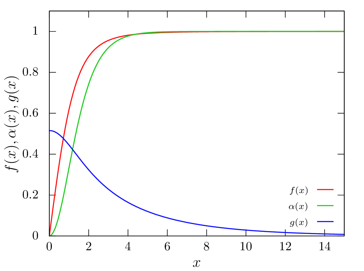
Figure 2: The field configuration of $f(x)$ (red), $\alpha(x)$ (green) and $g(x)$ (blue) with $\gamma=0.05$, $\beta_{\varphi}=\beta_{\sigma}=1$ and $\beta_{\varphi\sigma}=0.49$ (left-hand plot) and $\beta_{\varphi\sigma}=0.30$ (right-hand plot). Note that $g(x)$ in the right-hand plot is too small to be seen.

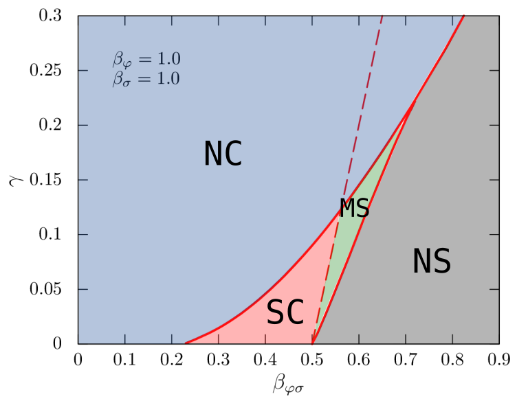
Figure 3: Regions of viability of strings in the $(\beta_{\varphi\sigma},\gamma)$ plane for $\beta_{\varphi}=\beta_{\sigma}=1$. The viable parameter region for a superconducting string is the red region labelled “SC” corresponding to field profiles as in the left-hand plot of Fig. (2). Strings form without a condensate in the blue region labelled “NC”. The corresponding field profiles are shown in the right-hand plot of Fig. (2), with $g(x)$ negligibly small. No string solutions (NS) exist in the grey region labelled “NS”. This region is where one is unable to obtain plausible field profiles which satisfy the boundary conditions (20) in the asymptotic region. Metastable strings (“MS”) form in the small region separated from region “SC” by the dashed line (defined by $\gamma=2\beta_{\varphi\sigma}-\sqrt{\beta_{\varphi}\beta_{\sigma}}$); in this region, superconducting strings are not stable against fluctuations.

The desirable field configurations of $f(x)$, $\alpha(x)$ and $g(x)$ are shown in the left-hand plot of Fig. 2, where $(\beta_{\varphi},\beta_{\sigma},\beta_{\varphi\sigma},\gamma)=(1,1,0.49,0.05)$. This parameter set yields a vortex solution on which $\sigma\propto g$ takes a non-zero value in the string core. In contrast, when $\beta_{\varphi\sigma}$ is small, the current-carrier $\sigma$ no longer condenses on the string, as shown in the right-hand plot of Fig. 2, where we set $\beta_{\varphi\sigma}=0.30$. This string behaves as an Abelian-Higgs string. In this case, the difference between $\widetilde{V}_{\rm eff}(C)$ and $\widetilde{V}_{\rm eff}(A)$ is too small to compensate for the increase in the gradient energy $\sim|\partial_{x}\sigma|^{2}$.

The regions of viability for superconducting strings and non-superconducting strings, obtained by solving Eqs. (9)-(11), in the range $0\leq\gamma\leq 0.3$ and $0\leq\beta_{\varphi\sigma}\leq 0.9$, with $\beta_{\varphi}=\beta_{\sigma}=1$ are shown in Fig. 3. In Appendix B we report on the cases with $\beta_{\sigma}=0.5$ and $1.0$ and $\beta_{\varphi}=0.1,\,0.5$ and $1.0$.

Superconducting strings (with field profiles as in the left-hand plot of Fig. 2) are obtained in the region labelled “SC”. This region is separated from a neighboring region labelled “MS” in which strings are in a meta-stable state. The line separating the two regions is given by $\gamma=2\beta_{\varphi\sigma}-\sqrt{\beta_{\varphi}\beta_{\sigma}}$. As discussed in Section II.3, to the right of the dashed line of Fig. 3, extremum [B] (see Fig. 1) is not the global minimum of the potential. This is why a superconducting string solution in the “MS” region is meta-stable. For small $\beta_{\varphi\sigma}$ or large $\gamma$, strings can form, but no condensate can be obtained (region “NC” in Fig. 3). The corresponding field profiles are shown in the right-hand plot of Fig. 2 with $g(x)$ suppressed to a level of order $10^{-10}$. For large $\beta_{\varphi\sigma}$, strings do not form (region “NS” in Fig. 3). In this region, one cannot obtain field profiles satisfying the boundary conditions (20) in the asymptotic region. In fact, in this region, the potential energy at extremum [C] in Fig. 1 becomes large and negative.

Note that the numerical study conducted in this section of the paper, which is restricted to the case of static string configurations, reveals that there exists sharp transitions between the “NC”, “SC” and “NS” regions. These transitions are represented by solid red lines. Note also that our study is not able to resolve the transition between the “SC” and “MS” regions, which instead stems from the analysis of Section II.3. The expression for the boundary of the region in which a string forms but no condensate forms (region “NC”), obtained by considering the gradient energy as well as the potential energy of a superconducting string, is derived in Appendix C.

While the analysis in this subsection was restricted to static strings, in the following section, we perform dynamical simulations of colliding strings starting from the static superconducting string solutions in the “SC” region.

III Simulation setup

Let us now consider the collision of two moving strings. An individual axisymmetric static vortex solution is obtained by solving Eq. 9 to Eq. 11 with the boundary conditions given in Eq. 20. We then obtain a moving string with velocity $v$ and angle $\alpha$ by performing a Lorentz transformation, as explained in Appendix D. These moving strings are placed in the computational domain as a superposition of the field configurations given in Eq. 41. A diagram depicting the initial string configuration is shown in Fig. 4. The coordinate origin is at the centre of the domain. It is labelled $O$. The strings have the same initial velocity, $v$, and move along the $x$-axis. For later convenience, we define hyper-surfaces $\Sigma_{I}$ for $I=x,y$ and $z$, as the surface perpendicular to the $I$-axis. The collision angle $\alpha$ is defined as the angle between two colliding strings projected onto the surface $\Sigma_{x}$ at $x=0$. As seen along the $x$-axis, towards positive values of $x$, the initial configuration and the angle $\alpha$ are shown in Fig. 5.

We define parallel and anti-parallel strings as the vortex solutions given in Eq. 6 to Eq. 8 with ${\rm sign}(n)={\rm sign}(K)$ and ${\rm sign}(n)=-{\rm sign}(K)$, respectively. In other words, the parallel ($p$) string is a string such that the direction of the magnetic flux, $\boldsymbol{B}:=\nabla\times\boldsymbol{A}$, and the direction of the conserved current, $\boldsymbol{j}^{\sigma}$, are parallel to each other while for the anti-parallel ($a$) string, they are anti-parallel to each other. We can consider three combinations: $(p,p)$, $(p,a)$ and $(a,a)$, as shown in Fig. 5. The solid arrow indicates the direction of $\boldsymbol{B}$, and the triple arrow is that of $\boldsymbol{j}^{\sigma}$, defined in Eq. 13.

In all simulation runs, we assume $\beta_{\varphi}=\beta_{\sigma}=1$ for simplicity. As we mentioned in Section II.3, stable superconducting strings can be obtained in a restricted region of the $\gamma$–$\beta_{\varphi\sigma}$ plane (recall that $\gamma=K^{2}-\Omega^{2}+\mu_{\sigma}^{2}$). Hence we can fix $\Omega=0$ without a loss of generality. We then vary other model parameters, $K$, $\mu_{\sigma}^{2}$ and $\beta_{\varphi\sigma}$. Then we vary the kinematical parameters of strings, the collision velocity $v$ and the collision angle $\alpha$.

For each simulation, we solve the dynamical equations Eq. 3 to Eq. 5 in Cartesian coordinates. The strings are assumed to extend infinitely outside the computational domain. To realise this, we use Eq. 41 as the boundary condition.

We use the Leap-Frog method in the time domain and approximate the spatial derivatives using second-order central finite differences. For consistency with the boundary conditions, each simulation ends before the result of the collision reaches the boundaries of the computational domain. We compute the optimal size of the computational domain by considering the velocity of strings and the collision angle. For details, see Appendix E.

Finally, we classify the final configuration of strings after the collision based on the criteria introduced in Section V.1.

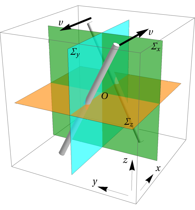
Figure 4: Computational domain and initial layout of the strings. $\Sigma_{I}$ for $I=x,y,z$ represents the plane perpendicular to $I$-axis. The strings moves along the $x$-axis with velocity $v$.

Figure 5: The solid arrow represents the direction of $\boldsymbol{B}:=\nabla\times\boldsymbol{A}$, which indicates the winding of a string (the upward arrow represents $n>0$). The triple arrow represents the direction of the conserved current, $\boldsymbol{j}^{\sigma}$ (the upward arrow represents $K>0$). A string with $\boldsymbol{B}\parallel\boldsymbol{j}^{\sigma}$ is a parallel ($p$) string and a string with $\boldsymbol{B}\parallel-\boldsymbol{j}^{\sigma}$ is an anti-parallel ($a$) string. We consider the three following pairs of strings: $(p,p)$, $(p,a)$ and $(a,a)$.

IV Final states of colliding strings

IV.1 Regular intercommutation

Let us first illustrate the familiar intercommutation process. We simulate a $(p,p)$ pair with model parameters $(\beta_{\varphi\sigma},\mu_{\sigma}^{2},K^{2})=(0.45,0.01,0.04)$ and $v/c=0.5,\,\alpha=0.2\pi$. In Fig. 6, the isosurface defined by $|\varphi|=\eta/2$ at $t=0,~{}17.5/(e\eta),~{}35/(e\eta)$ and $70/(e\eta)$ is shown in the first four 3D surface plots while the isosurface defined by $|j^{\sigma}_{i}|=0.01\eta/e$ at $t=70/(e\eta)$ is shown in the fifth 3D surface plot. Note that unless otherwise specified, in Fig. 6 to Fig. 9, the $z$-axis points upward in the vertical direction, the $x$-axis is oriented outwards and the $y$-axis points from left to right.

Intercommutation occurs at $t\approx 17.5/(e\eta)$ (in the second panel from the left), after which the strings move away from each other. This process is familiar in the Abelian-Higgs model in the absence of $\sigma$. The fifth plot of Fig. 6 shows that the current $j^{\sigma}_{\mu}$ on the reconnected strings survives the collision process. We shall discuss the evolution of the current during the collision process in  Section IV.5.

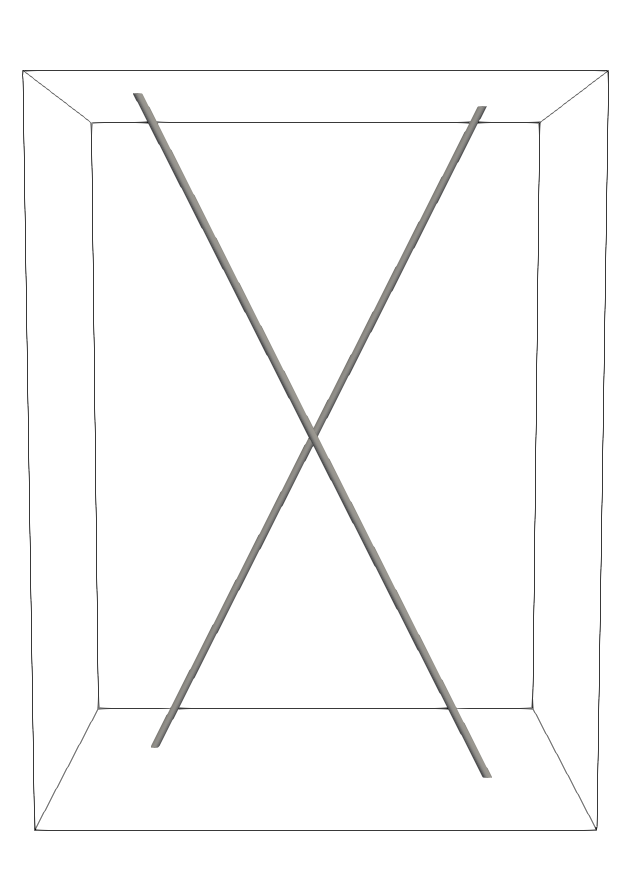
(a)

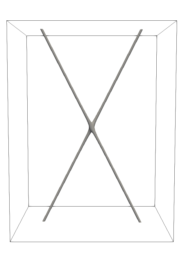
(b)

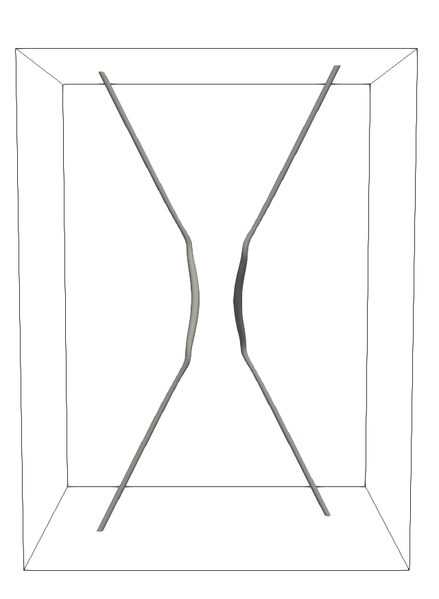
(c)

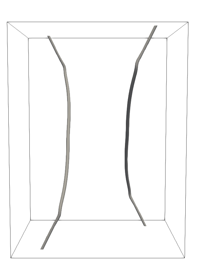
(d)

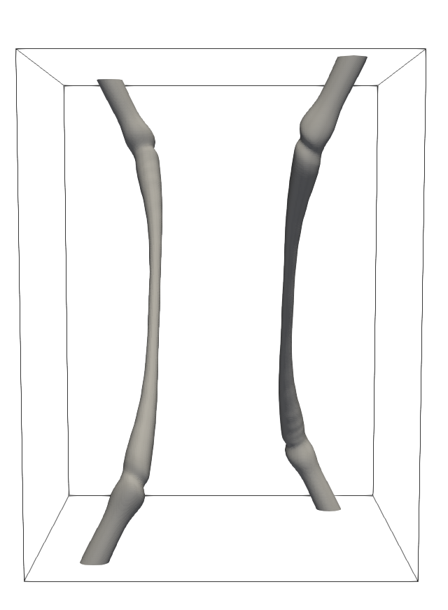
(e)

Figure 6: An example of the reconnection of strings with $(\beta_{\varphi\sigma},\mu_{\sigma}^{2},K^{2})=(0.49,0.01,0.04)$ and $v/c=0.5,\alpha=0.2\pi$. The panels (a)–(d) show the isosurface with $|\varphi|=\eta/2$ at $t=0,~{}17.5/(e\eta),~{}35.0/(e\eta),~{}70/(e\eta)$, respectively; (e) the fifth 3D surface plot shows the isosurface with $|j_{i}^{\sigma}|=0.01\eta/e$ at $t=70/(e\eta)$.

IV.2 Bound states

An interesting property of colliding strings is the possible formation of bound states ending at string Y-junctions. This phenomenon is known to appear in Type-I Abelian-Higgs strings where the gauge coupling is stronger than the self-coupling of the scalar field. In our setup, this corresponds to $\beta_{\varphi}<1$ and $\beta_{\varphi\sigma}=0$ [150, 94]. We find that superconducting strings, i.e. strings with $\beta_{\varphi\sigma}>0$, can form bound states even when $\beta_{\varphi}=1$. Indeed, while in the context of the Abelian-Higgs model with $\beta_{\varphi}=1$, no interactions between strings exist because the forces due to the gauge interaction and the scalar interaction balance each other out, in the case of a superconducting string and in the presence of the extra field $\sigma$, the balance of forces is modified, and bound states will form even when $\beta_{\varphi}=1$, as long as we set a relatively small velocity and small collision angle.

An example of a bound state formation for a $(p,p)$ pair is shown in Fig. 7. While the model parameters are the same as those in the previous subsection, the kinematic parameters are $v/c=0.2$ and $\alpha=0.1\pi$. The reconnection occurs soon after the collision, but the strong coupling between strings forms the bound state with Y-junctions at $t\approx 75/(e\eta)$. The length of the bound state is expected to grow with time until the string tension interrupts the development of the two Y-junctions.

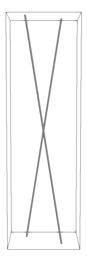
(a)

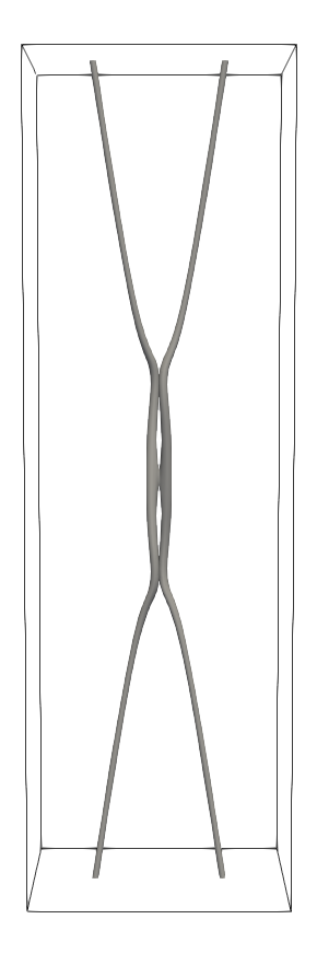
(b)

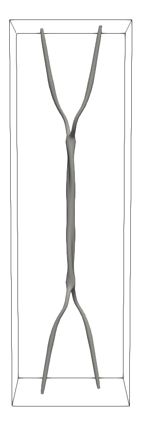
(c)

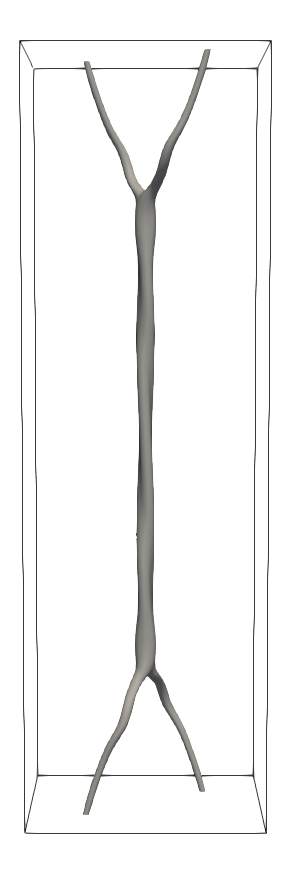
(d)

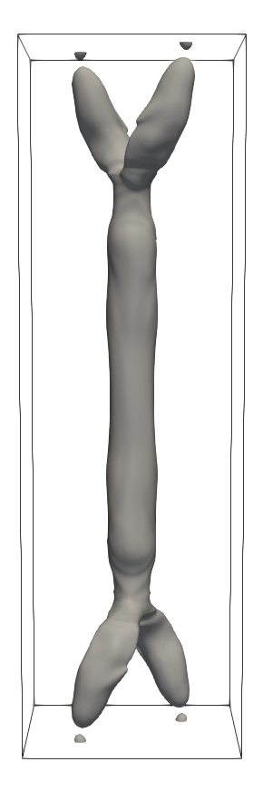
(e)

Figure 7: A bound state is formed after the collision with the same model parameters as used in Fig. 6, $(\beta_{\varphi\sigma},\mu_{\sigma}^{2},K^{2})=(0.49,0.01,0.04)$, but with different kinematical parameters, $v/c=0.2,\alpha=0.1\pi$. The panels (a)–(d) show the isosurface $|\varphi|=0.5\eta$ at $t=0,50/(e\eta),\,75/(e\eta)$ and $100/(e\eta)$, respectively; (e) shows $|j_{i}^{\sigma}|=0.01\eta/e$ at $t=100/(e\eta)$.

IV.3 Double intercommutation

In a collision process, strings may intercommute once, as already discussed, or intercommute multiple times [83, 84]. If an even number of intercommutations occur, the strings will consequently “pass” through each other. This phenomenon was first reported for Abelian-Higgs strings with large velocities ($v/c\gtrsim 0.9$) and large collision angles ($\alpha\sim\pi/2$) [83]. Here we discuss double intercommutation, as intercommutations occurring more than twice are rare.

In Fig. 8, we display the case of a $(p,p)$ pair with $(\beta_{\varphi\sigma},\mu_{\sigma}^{2},K^{2})=(0.49,0.01,0.04)$, $v/c=0.5$ and $\alpha=0.14\pi$. In the plots (a)-(d), the 3D surface plots are taken at $t=0,~{}32.5/(e\eta),~{}42.5/(e\eta)$ and $70/(e\eta)$ respectively. The strings collide and intercommute in plot (b), similarly to what is shown in plot (c) of Fig. 6. Then, they intercommute once more in plot (c) and “pass” through one another; see plot (d). By looking at the locations of the string endpoints at the top and bottom boundaries of the field theory computational domain, one can confirm that the strings intercommute twice and “pass” through each other. Note that the currents survive the double intercommutation process, as shown in (e).

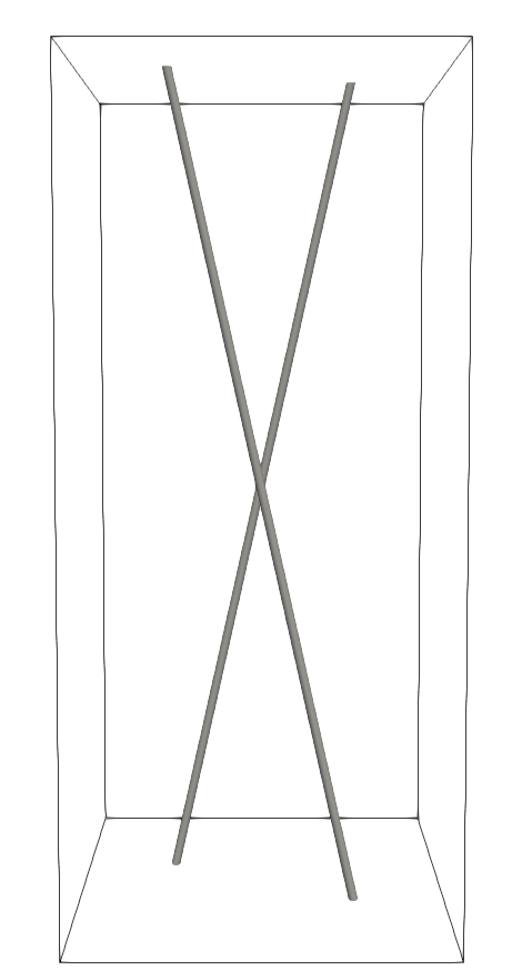
(b)

(b)

(c)

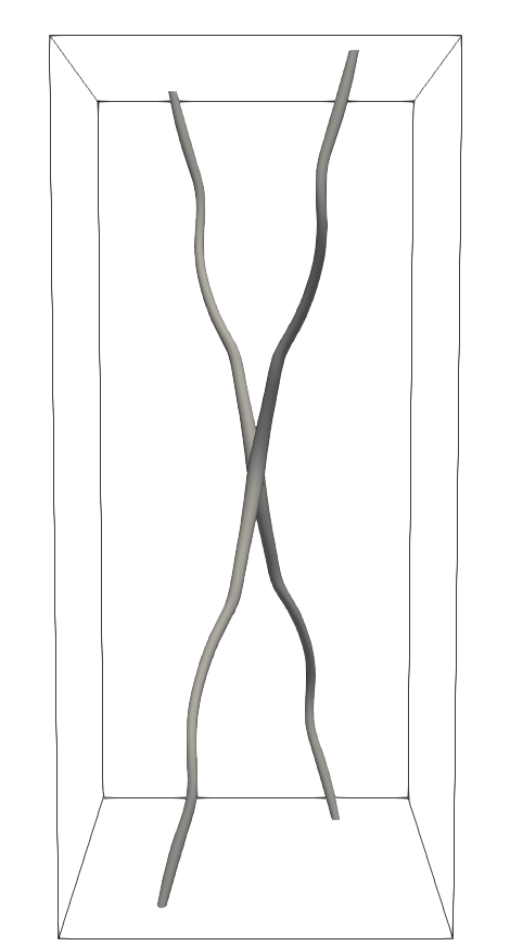
(d)

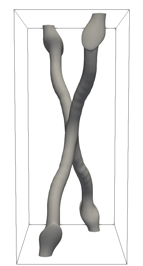
(e)

Figure 8: Double intercommutation process with $(\beta_{\varphi\sigma},\mu_{\sigma}^{2},K^{2})=(0.49,0.01,0.04)$ and $v/c=0.5,\alpha=0.14\pi$. As a result, they slip through each other. Plots (a)-(d) show the isosurfaces defined by $|\varphi|=\eta/2$ at $t=0,32.5/(e\eta),42.5/(e\eta)$ and $70/(e\eta)$, respectively; Plot (e) shows the isosurface $|j^{\sigma}_{i}|=0.01\eta/e$ at $t=70/(e\eta)$.

IV.4 Expanding bubble

Finally, superconducting string collisions can result in the nucleation of a bubble. As mentioned in Section II.3 and Section II.4, static strings for which the parameters of the effective potential are in the “MS” region of Fig. 3 are unstable. Here, we consider a $(p,p)$ pair with $(\beta_{\varphi\sigma},\mu_{\sigma}^{2},K^{2})=(0.51,0.01,0.04)$, i.e. $\gamma=0.05$, $v/c=0.6$ and $\alpha=0.22\pi$. Although this set of parameters belongs to the “SC” region of Fig. 3, the dynamical simulation reveals that the string configuration is broken after the collision, as shown in Fig. 9. The strings collide at $t=15/(e\eta)$ in plot (a) and intercommute in plot (b). The reconnected segments then come into contact once more at $t=32.5/(e\eta)$ in plot (c). The reconnected region then expands, see plot (d). In plot (e), we plot the corresponding current amplitude at $t=32.5/(e\eta)$. Note that they merge into a single current.

As pointed out in Section II.3, the stable vortex solution cannot be obtained if the vacuum [C] is energetically favoured (see Fig. 1). Indeed, in such a case, the volume where the fields lie at [C] in the interior of the string grows with time, so that the string configuration is broken, as shown in the right plot of Fig. 9. According to Fig. 3, the case with $\beta_{\varphi\sigma}=0.51$ belongs to the “NS” region. Our numerical result suggests that the colliding string has, locally, entered this region.

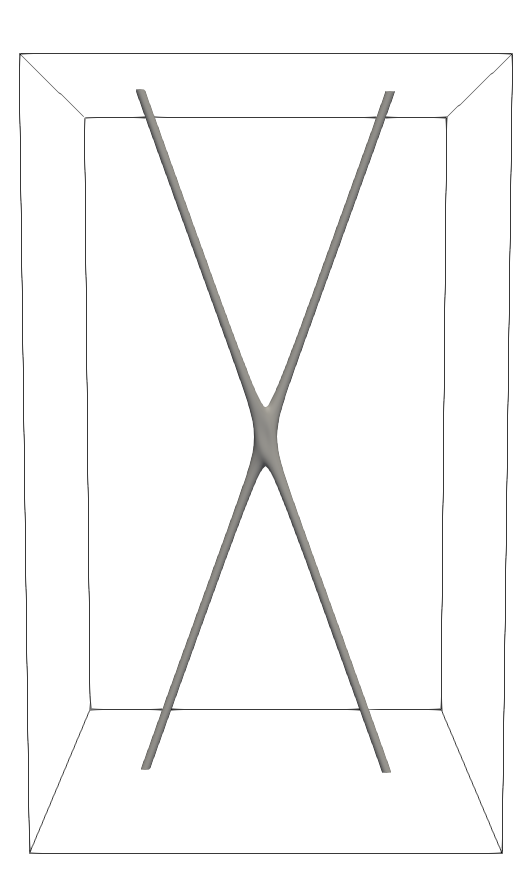
(a)

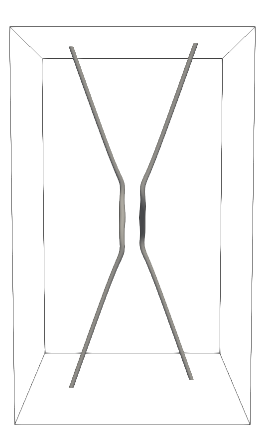
(b)

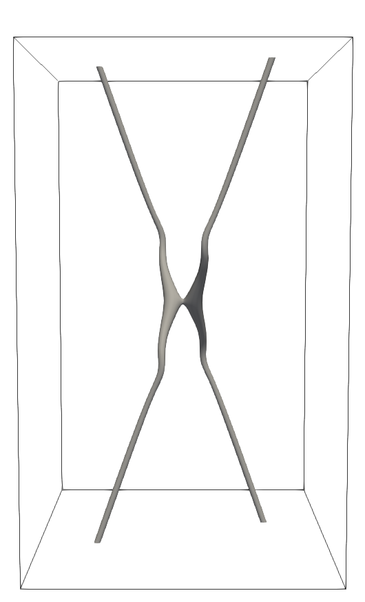
(c)

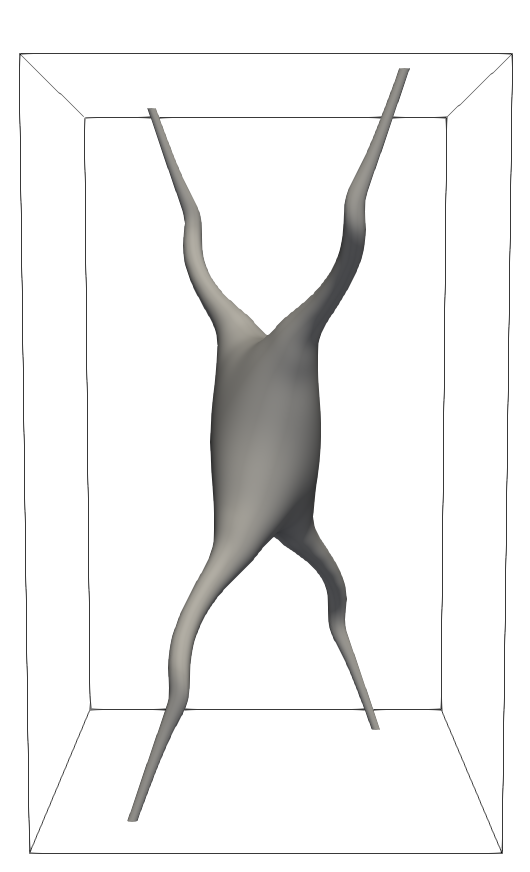
(d)

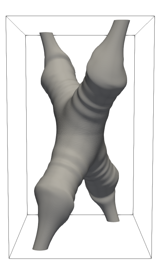
(e)

Figure 9: For $(\beta_{\varphi\sigma},\mu_{\sigma}^{2},K^{2})=(0.51,0.01,0.04)$, $v/c=0.6$ and $\alpha=0.22\pi$ the interior of the string expands and then the string configuration breaks down. From left to right, each 3D surface plot shows the isosurface $|\varphi|=\eta/2$ at $t=15/(e\eta),~{}25/(e\eta),~{}32.5/(e\eta)$ and $65/(e\eta)$ while (e) shows $|j^{\sigma}_{i}|=0.01\eta/e$ at $t=65/(e\eta)$.

IV.5 Current on strings after collision

Figure 10: The time evolution of the current on $\Sigma_{z}$ with $\alpha=0.02\pi$ (red), $0.14\pi$ (green), $0.30\pi$ (blue) and $0.46\pi$ (magenta) for a $(p,p)$ pair with $(\beta_{\varphi\sigma},\mu_{\sigma}^{2},K^{2})=(0.49,0.01,0.04)$ and $v/c=0.1$. At the initial time, $J_{z}(0)\approx 2.4\eta/e$. After the collision, the current on the strings fluctuates significantly. It can sometimes take on negative values.

To quantify the magnitude of the current of $\sigma$ on the strings after the collision, we define the current evaluated on the hypersurface $\Sigma_{I}$ for $I=x,y,z$, defined in Fig. 4, as

$$J_{I}:=\int j^{\sigma}_{\mu}\,d\Sigma^{\mu}_{I},$$ (21)

where $j^{\sigma}_{\mu}$ is the conserved current defined in Eq. 13 and $d\Sigma^{\mu}_{I}$ is the surface element of the hypersurface $\Sigma_{I}$. For a $(p,p)$ pair, in the case of $(\beta_{\varphi\sigma},\mu_{\sigma}^{2},K^{2})=(0.49,0.01,0.04)$, the initial currents on the string flow in the positive direction across $\Sigma_{z}$, and its magnitude is $J_{z}(0)\approx 2.4\eta/e$. There is no current across $\Sigma_{x}$. The currents of each string flow in opposite directions and with the same magnitude across $\Sigma_{y}$, so that the net currents $J_{x}=J_{y}=0$.

In Fig. 10, we show the time evolution of the current $J_{z}(t)$ for $\alpha=0.02\pi$ (red), $0.14\pi$ (green), $0.30\pi$ (blue) and $0.46\pi$ (magenta) with $v/c=0.1$ for a $(p,p)$ pair. The final configurations for $\alpha=0.02\pi,0.14\pi$ and $0.30\pi$ are bound states, while the choice $\alpha=0.46\pi$ results in regular intercommutation. We find that, after the collision, the current on the strings fluctuates significantly and can sometimes take on negative values. We can confirm that finite box size effects do not affect these findings. However, we cannot confirm whether the current will be sustained in the final state at large $t$ in the present numerical setup. To confirm it, one would need a longer simulation with a larger simulation box.

V Classification and phase diagrams

V.1 Classification

There is a total of five possible outcomes for superconducting string collisions. A summary of these final states is shown in Fig. 11. The first four states, (a) to (d), were discussed in previous sections. The last one, state (e), is one for which the outcome of the collision is an indeterminate final string state, which, for longer simulation times, may evolve into either (c) or (d).

Let us now introduce some criteria with which we can classify the final states of colliding strings, using the simulated end states of $\varphi(t_{\rm end},\boldsymbol{x})$ and $\sigma(t_{\rm end},\boldsymbol{x})$, at $t_{\rm end}$. Our code computes, at $t_{\rm end}$, the surface areas for which $|\varphi|<\eta/2$ on $\Sigma_{x}$, $\Sigma_{y}$ and $\Sigma_{z}$, see Fig. 4. Those surface areas are denoted by $S_{x},S_{y}$ and $S_{z}$, respectively. If the strings undergo regular intercommutation, $S_{x}\neq 0,S_{y}=0$ and $S_{z}\neq 0$ for all $\alpha$. Indeed, since the strings have velocities along the $x$-axis and momentum is conserved after the collision, the strings must cross $\Sigma_{x}$, while it is the intercommutation process that results in $S_{y}=0$ and $S_{z}\neq 0$ for this particular configuration of string collision. This is confirmed by Fig. 6.

If the strings undergo double intercommutation, they “pass” through each other such that the final string configuration is identical to the starting configuration. In this case, $S_{x}=0$, see plot (b) in Fig. 11.

If $S_{x},S_{y}$ and $S_{z}$ are all non-zero, the strings either create a bound state or become unstable and the volume for $|\varphi|<\eta/2$ grows with time. If the strings form a bound state, the final configuration is parallel to the $z$-axis. Hence $S_{z}$ should be much smaller than $S_{x}$ and $S_{y}$ (plot (c) in Fig. 11). Instead, if $S_{x},S_{y}$ and $S_{z}$ are comparable, the final state would be like plot (d) or (e) in Fig. 11 and thus corresponds to bubble nucleation or an indeterminate string state.

To distinguish between (c) and (d) or (e), we introduce an ellipticity parameter defined as $e_{z}\equiv S_{z}^{-1}/(S_{x}^{-2}+S_{y}^{-2}+S_{z}^{-2})^{1/2}$. If the strings are bounded along the $z$-axis, $e_{z}\sim 1$. In what follows, we consider the final string state to be a bound state when $e_{z}\geq e_{z,{\rm crit}}=0.9$.

As mentioned before, because simulation time is limited, some end configurations at $t_{\rm end}$ see plot (e) of Fig. 11 are not in their definitive state and could evolve into either (c) or (d) for longer simulation times. These strings are in an indeterminate state at $t_{\rm end}$. To decide whether a final string configuration is in state (d) or (e), we introduce the effective volume $V=\sqrt{S_{x}S_{y}S_{z}}$, and consider final states with $e_{z}<e_{z,{\rm crit}}$ and $V\geq V_{\rm crit}=3\times 10^{4}\eta^{-3}$ to be expanding bubbles, while if $V<V_{\rm crit}$, we consider them to be indeterminate string states.

The classification of the final states is summarized Table 1. In the following, we use, throughout, the critical values $e_{z,{\rm crit}}=0.9$ and $V_{\rm crit}=3\times 10^{4}\eta^{-3}$ mentioned above. These criteria, while they have no rigorous physical motivation, are useful for the classification of strings end states into types (a) to (e). Note that slight changes in these parameters do not significantly affect our findings.

Note that we do not discuss whether currents remain on the string after the collision. In the previous section, we saw cases for which the current disappears after the collision but we believe this phenomenon to be transient, with a non-zero current re-established for a simulation with increased duration and a larger computational domain. While in principle the final state of the current is of interest, the current on the strings after the collision continues to fluctuate significantly in our simulations, see Fig. 10. For this reason, in what follows, we do not report on the current’s final configuration. Finally, we would like to point out that bound states may also be transient and may disappear under the effect of the string tension for longer simulation times, particularly for cases in which the bound state is formed on the edge of its region of viability in parameter space.

Criteria	Classification	Critical values
$S_{x}\neq 0$, $S_{y}=0$ and $S_{z}\neq 0$	regular intercommutation	–
$S_{x}=0$	double intercommutation	–
$e_{z}\geq e_{z,\mathrm{crit}}$	bound state	$e_{z,{\rm crit}}=0.9$
$e_{z}<e_{z,\mathrm{crit}}$ and $V>V_{\mathrm{crit}}$	expanding bubble	$V_{\rm crit}=3\times 10^{4}\eta^{-3}$
none of the above	indeterminate state	–

Table 1: Criteria used in the classification of string collision final states.

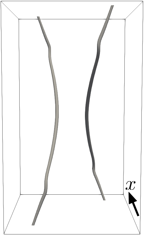
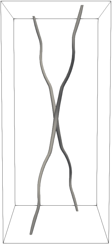
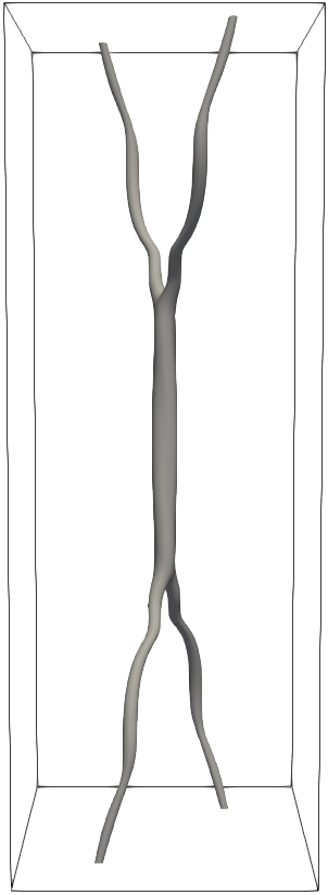
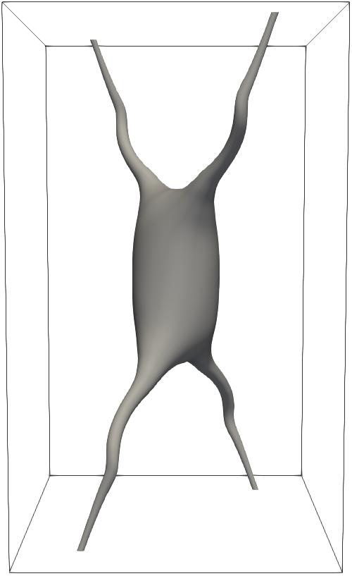
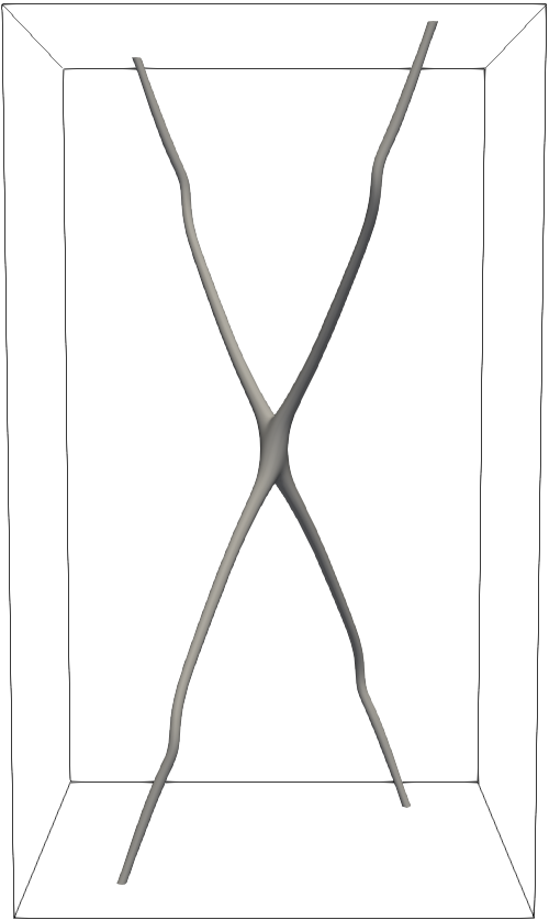
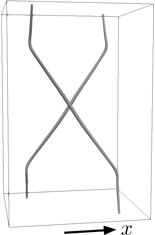
(a)

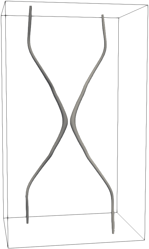
(b)

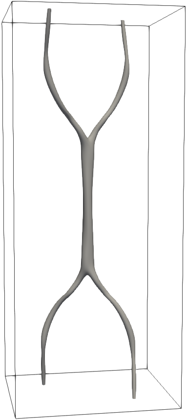
(c)

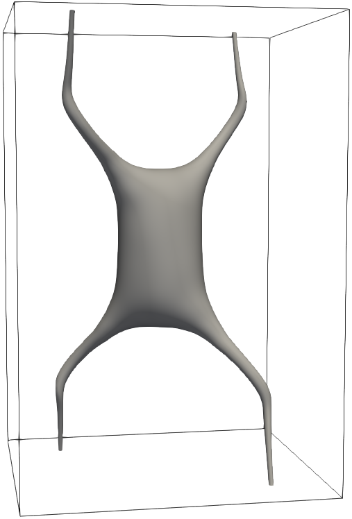
(d)

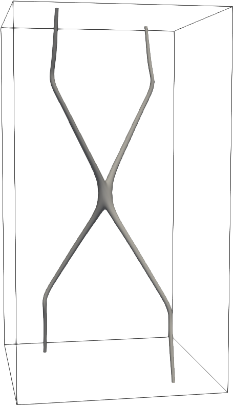
(e)

Figure 11: Superconducting string collision outcomes: (a) regular intercommutation, (b) double intercommutation, (c) bound state with Y-junctions, (d) unstable configuration, and (e) indeterminate final state. Note that the lower plots show the upper panels rotated 90 degrees around the $z$-axis, as indicated by the arrows representing the $x$-axis.

V.2 Phase diagram

In this section, we report on the final states resulting from the collision of superconducting strings in the $(v,\alpha)$ plane. We consider six sets of model parameters, listed in Table 2. In Model I, the parameters are the same as the ones used in Section IV.3. In Model II, $\beta_{\varphi\sigma}$ is taken to be slightly larger than in Model I. In Models III and IV, we set $K^{2}$ to be respectively smaller and larger than in Models I and II. In Model V, $\beta_{\varphi\sigma}$ is smaller than in Model III. Finally, in model VI, $K^{2}$ and $\mu_{\sigma}^{2}$ are interchanged with those in Model IV, while keeping $\gamma=0.08$.

We vary the collision velocity $v/c$ from $0.1$ to $0.9$ in steps $\Delta(v/c)=0.05$, and the collision angle $\alpha$ (see Fig. 5 for the definition of $\alpha$) from $0.02\,\pi$ to $0.46\,\pi$ in steps $\Delta\alpha=0.04\,\pi$. In Models I and II, we also consider angles $\alpha$ in the range $0.58\pi\leq\alpha\leq 0.98\pi$, with $\Delta\alpha=0.08\,\pi$. We classify the final configurations according to Table 1.

V.2.1 Model I

The phase diagram for Model I is shown in Fig. 12 for $(p,p)$ and $(p,a)$-type string pairs (see Section III for details). Strings with $v/c\lesssim 0.5$ and $\alpha\lesssim 0.3\,\pi$ form bound states. This is similar to the outcome of the collisions between Type-I Abelian-Higgs strings with $e^{2}>\lambda/2$ [94]. Strings with $v/c\sim 0.5$ and $\alpha\sim 0.2\pi$ pass through each other via double intercommutation. This behaviour is observed in Type-I/II Abelian-Higgs strings only for strings with large velocities [83, 84]. Note that while bound states form in a wide range of velocities and angles, double intercommutation occurs only in a restricted region of the kinematic parameter space.

As is well known, in a bound state, Y-junctions may form [86, 87, 88, 89, 90, 91, 92, 93]. At such junctions, the string tension in the two outer strings may unbind the bound string state. Whether this unbinding is observed or not depends on the duration of the simulation. For this reason, the border between the regions of regular intercommutation and bound states comprises some indeterminate string states.

Model	I	II	III	IV	V	VI
$\beta_{\varphi\sigma}$	0.49	0.51	0.49	0.49	0.40	0.49
$\mu_{\sigma}^{2}$	0.01	0.01	0.01	0.01	0.01	0.07
$K^{2}$	0.04	0.04	0.02	0.07	0.02	0.01
$\gamma$	0.05	0.05	0.03	0.08	0.03	0.08
String type in Fig. 3	SC	MS	SC	SC	SC	SC

Table 2: Model parameters. Throughout the simulations, we fix $\beta_{\varphi}=\beta_{\sigma}=1$ and $\Omega=0$. Note that while the phase diagrams obtained are not sensitive to the value of $\Omega$, they are sensitive to the difference $K^{2}-\Omega^{2}$.

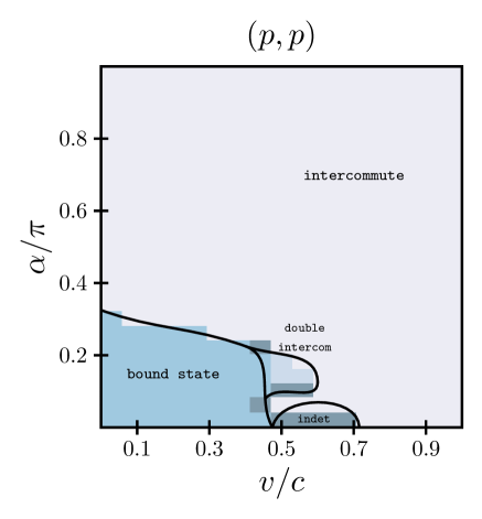
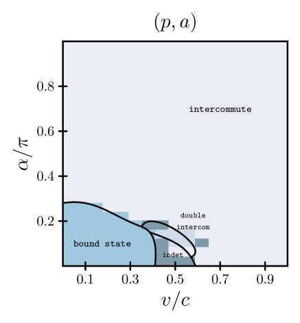
Figure 12: The phase diagram of the colliding strings for Model I, with $(\beta_{\varphi},\beta_{\varphi\sigma},\beta_{\sigma},\mu_{\sigma}^{2},K^{2})=(1.0,0.49,1.0,0.01,0.04)$. The left panel is $(p,p)$ and the right one is $(p,a)$.

One also finds that collisions with large angles, $\alpha>\pi/2$, result in regular intercommutation for all values of the velocity. If the collision angle is large, the curvature of the outgoing strings around the impact point is significant, and the string velocity near the impact point is large. For this reason, in such a configuration, no bound state can be formed, and no double intercommutation can occur.

Note that the phase diagram for $(a,a)$-type strings is identical to the one for $(p,p)$-type strings in Fig. 12. This means that while the relative orientation of the currents affects the outcome of superconducting string collisions, the relative orientation of the current and the winding is not essential. This also holds true for models II to VI.

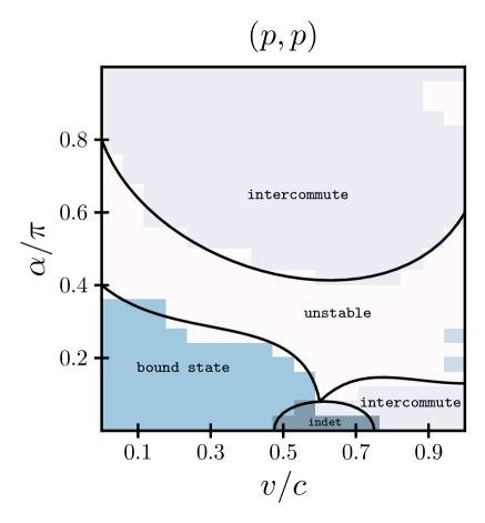
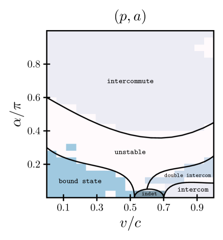
Figure 13: Phase diagram of the colliding strings for Model II, with $(\beta_{\varphi},\beta_{\varphi\sigma},\beta_{\sigma},\mu_{\sigma}^{2},K^{2})=(1.0,0.51,1.0,0.01,0.04)$. The left and right-hand plots correspond to $(p,p)$ and $(p,a)$-type string pairs, respectively.

V.2.2 Model II

Let us now consider the collisions of strings whose parameters belong to the region of Fig. 3 labelled “MS”. In this region, the extremum [C] in Fig. 1 becomes the global minimum (see lower plot). Strings in this region of parameter space are dynamically unstable, which means that collisions of such strings can lead to expanding bubbles around the impact point (see Section IV.4). This is confirmed by the results of the dynamical simulations, see Fig. 13, which demonstrate that the collisions of strings belonging to model II form bubbles in a large part of the kinematic phase space when $\alpha\lesssim\pi/2$, see Fig. 13 while they intercommute when $\alpha\gtrsim\pi/2$.

As can be seen from Fig. 3, strings with $\gamma\geq\min\left(0,2\beta_{\varphi\sigma}-\sqrt{\beta_{\varphi}\beta_{\sigma}}\right)$ for values $\beta_{\varphi\sigma}\leq 0.5$ belong to region “SC”. In a hypothetical bound state resulting from a collision of two model II strings, the total current is given by $2K\cos(\alpha/2)$. Given the constraint on $\gamma$ given above and its definition ($\gamma=K^{2}+\mu_{\sigma}^{2}$), one can deduce that the collision of strings in region “MS” can result in stable bound states for small angles $\alpha$. In addition, the interaction time will scale as the ratio of the string thickness, $d$, and the velocity of the incident strings, taken to be $v$. That is to say, the interaction time and the probability to form bound states will be greater for small velocities.

It is worth noting that the region in the $(v/c,\alpha/\pi)$ plane in which the result of the collision of model II strings is an unstable string state is greater for greater values of $\beta_{\varphi\sigma}$. This can be seen in Fig. 3 and from the constraint on $\gamma$ given in the preceding paragraph, and it is confirmed by a set of additional simulations (not shown) with $0.50\leq\beta_{\varphi\sigma}\leq 0.51$. In these simulations, the region of parameter space in which a collision results in the appearance of an unstable string state (in the form of an expanding bubble) is larger for large values of $\beta_{\varphi\sigma}$, while it shrinks considerably for $\beta_{\varphi\sigma}\lesssim 0.50$.

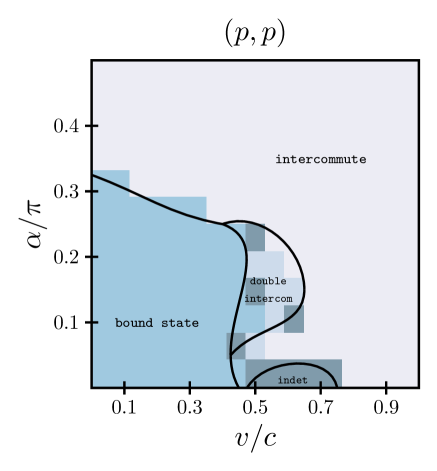
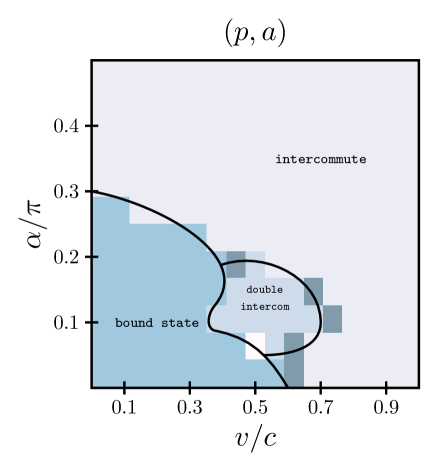
Figure 14: The phase diagram of the colliding strings for Model III, with $(\beta_{\varphi},\beta_{\varphi\sigma},\beta_{\sigma},\mu_{\sigma}^{2},K^{2})=(1.0,0.49,1.0,0.01,0.02)$.

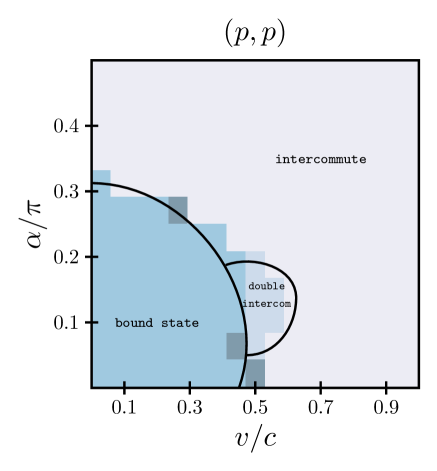
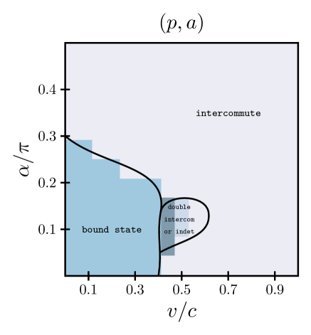
Figure 15: The phase diagram of the colliding strings for Model IV, with $(\beta_{\varphi},\beta_{\varphi\sigma},\beta_{\sigma},\mu_{\sigma}^{2},K^{2})=(1.0,0.49,1.0,0.01,0.07)$.

V.2.3 Model III & IV

In going from Model III to IV, the squared amplitude of the currents in the two colliding, $K^{2}$, is increased from 0.02 to 0.07. The corresponding phase diagrams are shown in Fig. 14 and Fig. 15, respectively, and are similar to the ones of Model I, see Fig. 12. In particular, strings intercommute in the usual way for all $\alpha>\pi/2$. For this reason, in Fig. 14 and Fig. 15, the phase plots are shown for the reduced range $0\leq\alpha\leq\pi/2$ rather than for the full range 0 to $\pi$. The similarity of these phase plots suggests that the initial current $K$ does not play an essential role in the outcome of the collision as long as $\beta_{\varphi\sigma}<0.5$. This applies especially to the regions in which bound states form and regular intercommutation occurs. We refer the reader to the discussion in Section V.2.2 for the case $\beta_{\varphi\sigma}>0.5$.

Note that the region of double intercommutation is smaller when the amplitude of the current in the colliding strings is larger. This is visible by comparing the results for model I and IV with those of model III. One can conclude that larger currents hinder the occurrence of double intercommutation and instead favor regular intercommutation and/or the formation of bound states.

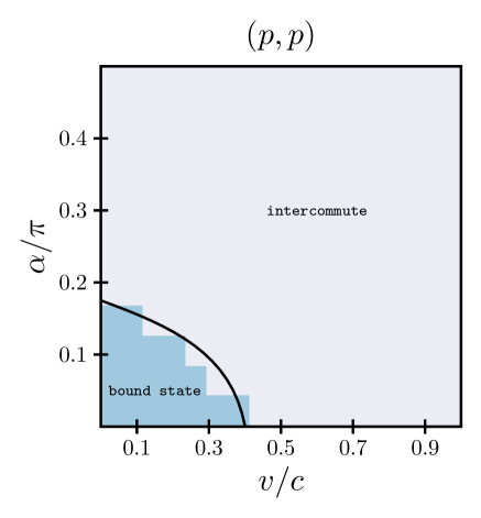
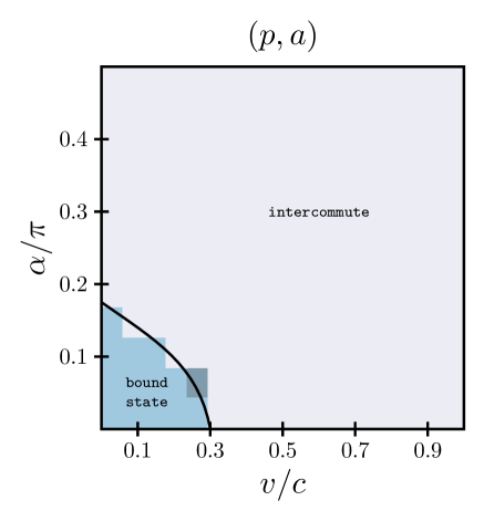
Figure 16: The phase diagram of the colliding strings for Model V, with $(\beta_{\varphi},\beta_{\varphi\sigma},\beta_{\sigma},\mu_{\sigma}^{2},K^{2})=(1.0,0.4,1.0,0.01,0.02)$.

V.2.4 Model V

Let us now study the influence of $\beta_{\varphi\sigma}$, the coupling constant between $\varphi$ and $\sigma$. To do so, we compare the results of Model III in Fig. 14 with those of Model V in Fig. 16. In going from Model III to Model V, $\beta_{\varphi\sigma}$ is decreased from 0.49 to 0.40, while all other parameters are kept identical. We find that bound states form less frequently for smaller $\beta_{\varphi\sigma}$ (Model V). This result is reasonable. Indeed, if we consider the limit $\beta_{\varphi\sigma}\to 0$, the strings are similar to critical Abelian-Higgs strings, which do not form bound states.

While in comparing Model I and III, we found that the size of the region in which bound states form is largely insensitive to $K$, here, we find, by comparing models III and V, that its size has a clear dependence on $\beta_{\varphi\sigma}$. We thus conclude that the parameter which determines whether bound states can form is the coupling $\beta_{\varphi\sigma}$.

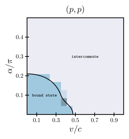
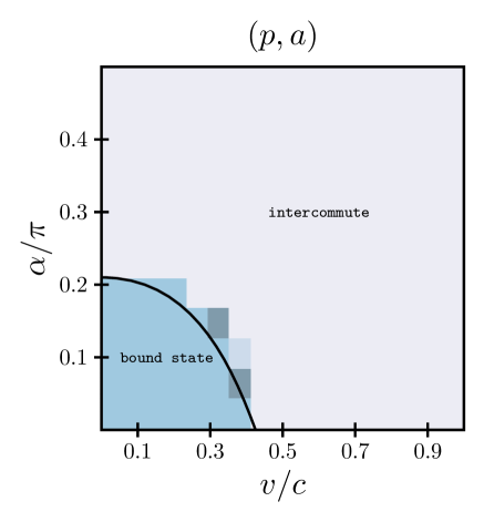
Figure 17: The phase diagram for the colliding strings of Model VI with $(\beta_{\varphi},\beta_{\varphi\sigma},\beta_{\sigma},\mu_{\sigma}^{2},K^{2})=(1.0,0.49,1.0,0.07,0.01)$.

V.2.5 Model VI

Finally, let us consider a case with large $\mu_{\sigma}^{2}$, the bare mass of $\sigma$. Note that Model IV (Fig. 15) and VI both have $\gamma=0.08$, with the values of $K$ and $\mu_{\sigma}$ interchanged. As explained in Section II.4, the stability of a straight and static string is determined by two parameters, $\beta_{\varphi\sigma}$ and $\gamma=K^{2}-\Omega^{2}+\mu_{\sigma}^{2}$ (recall that $\Omega=0$ in our simulations). While the individual values of $\mu_{\sigma}^{2}$ and $K^{2}$ do not play an essential role in the analysis of static strings, we find, by comparing the results of Model IV and Model VI, that the dynamical process does depend on $\mu_{\sigma}^{2}$ itself.

The phase diagram of Model VI is shown in Fig. 17. We find a significant decrease in the size of the region of kinematic parameter space in which bound states can form in Model VI, in comparison to Model IV. To explain this difference, we note, from Eq. 2, that the effective mass of $\sigma$, in the core of the string, is bounded from below by $\mu_{\sigma}$ ($m_{\sigma}$). Correspondingly, the length scale over which two strings interact, which is roughly given by the inverse of the effective mass, is bounded from above by $\mu_{\sigma}^{-1}$.

VI Conclusion

In this work, we studied the collision process of two superconducting strings using field-theoretic simulations. We considered a complex scalar field $\varphi(\boldsymbol{x},t)$ with its associated gauge field $A_{\mu}(\boldsymbol{x},t)$ and another complex scalar field $\sigma(\boldsymbol{x},t)$. This model has $U_{\rm local}(1)\times U_{\rm global}(1)$ symmetry, and the breaking of the $U_{\rm local}(1)$ symmetry leads to the formation of cosmic strings.

We first considered an Abrikosov-Nielsen-Olesen vortex solution on which the current-carrier $\sigma$ condenses. We solved the field equations numerically in order to obtain the field configuration and determine the region of parameter space in which strings are viable. The parameter space considered is the $(\beta_{\varphi\sigma},\gamma)$ plane, where $\beta_{\varphi\sigma}=\lambda_{\varphi\sigma}/2e^{2}$ is the coupling constant between $\varphi$ and $\sigma$, and $\gamma=K^{2}-\Omega^{2}+\mu_{\sigma}^{2}$ is the effective mass of $\sigma$ condensed on the string.

We then considered two straight current-carrying strings in a collision process. From the static string solutions, we performed a Lorentz transformation in order to obtain moving strings with velocity $v$ and relative angle $\alpha$. In a three-dimensional computational domain, we then performed dynamic simulations of the collision process. Using a set of criteria defined in Table 1 we classified the final string configuration after the collision. The results are summarised in the phase diagrams of  Fig. 12–Fig. 17 for the six sets of string parameters defined in Table 2.

While most colliding strings do intercommute in the same manner as in the Abelian-Higgs model in parts of the string parameter space and collision configuration space, we also found a variety of other final states depending on the model parameters and on the kinetics of the simulations. With a relatively small velocity, $v/c\lesssim 0.5$ and a small angle, $\alpha\lesssim 0.3\pi$, the colliding strings form a bound state; this is consistent with what can be observed in Type-I Abelian-Higgs strings. We also observe that two strings can pass through one another in a double intercommutation mechanism. This phenomenon is also observed in the collision of Type-I/II Abelian-Higgs strings at speeds close to $c$.

Furthermore, two strings with a relatively large $\beta_{\varphi\sigma}$ form an expanding bubble after the collision, and the string configuration breaks down. In the bubble’s interior, $\varphi$ and $\sigma$ lie at the extremum labelled [C], defined in Section II.3. Once a small segment of string around the impact point enters the region of string instability region in the $(\beta_{\varphi\sigma},\gamma)$ plane, it expands and tends to fill the entire 3D computational domain. This phenomenon can be observed only if $\beta_{\varphi\sigma}$ is larger than its critical value.

In summary, our numerical studies demonstrate that there exists a substantial variety of final string configurations in a dynamical current-carrying string collision process. This suggests that in a cosmological context, the evolution of the network of superconducting strings should be more complicated than that of Abelian-Higgs strings. It is therefore non-trivial that a superconducting string network would follow scaling laws similar to what is found in the Abelian-Higgs model [59, 60, 61, 62, 63, 64, 65, 66]. This being said, should the superconducting string network indeed follow a scaling law, the number density of superconducting strings may differ from the one found in the Abelian-Higgs case due to the formation of bound states and double intercommutation. This could leave a distinct characteristic imprint on the cosmic microwave background and gravitational wave background. Furthermore, if standard model particles or dark matter particles condense on strings, the resulting superconducting strings could generate fast radio bursts [151, 152] and could also be at the origin of gamma-ray bursts [153, 154].

Let us finally note that in the present study, the scalar field that condenses onto the string induces a long-range force, which enhances interactions with distant strings. The dynamics of the strings would change were the scalar field gauged, since its effect would then be confined around the strings [145]. We leave this type of superconducting string for a future study.

Appendix A Notations

We use the same model as used in Peter’s paper [109], but follow the different notations. The correspondence of the variables and parameters between the literature and ours is as follows:

$$\varphi=\frac{1}{\sqrt{2}}\Phi^{\rm Peter},\quad\sigma=\frac{1}{\sqrt{2}}\Sigma^{\rm Peter},\quad A_{\mu}=-\frac{1}{\sqrt{4\pi}}B_{\mu}^{\rm Peter},$$ (22)

$$e=\sqrt{4\pi}q^{\rm Peter},\quad\eta=\frac{1}{\sqrt{2}}\eta^{\rm Peter},\quad m_{\sigma}=\sqrt{2}m_{\sigma}^{\rm Peter},$$ (23)

$$\lambda_{\varphi}=2\lambda_{\phi}^{\rm Peter},\quad\lambda_{\varphi\sigma}=4f^{\rm Peter},\quad\lambda_{\sigma}=4\lambda_{\sigma}^{\rm Peter}.$$ (24)

The dimensionless parameters $\alpha_{i}$ ($i=1,2,3$) and $\widetilde{w}$, $\widetilde{q}$ defined in Ref. [109] can be represented by our notations,

$$\alpha_{1}=\frac{m_{\sigma}^{2}}{\lambda_{\sigma}\eta^{2}}=\frac{\mu_{\sigma}^{2}}{\beta_{\sigma}},\quad\alpha_{2}=\frac{\lambda_{\varphi\sigma}m_{\sigma}^{2}}{2\lambda_{\varphi}\lambda_{\sigma}\eta^{2}}=\frac{\beta_{\varphi\sigma}\mu_{\sigma}^{2}}{2\beta_{\varphi}\beta_{\sigma}},\quad\alpha_{3}=\frac{m_{\sigma}^{4}}{2\lambda_{\varphi}\lambda_{\sigma}\eta^{4}}=\frac{\mu_{\sigma}^{4}}{2\beta_{\varphi}\beta_{\sigma}},$$ (25)

$$\widetilde{q}^{2}=\frac{1}{4\pi\beta_{\varphi}},\quad\widetilde{w}=\frac{\mu_{\sigma}^{2}W}{2\beta_{\varphi}\beta_{\sigma}},$$ (26)

and we can rewrite $\beta_{\varphi},\beta_{\varphi\sigma},\beta_{\sigma}$ and $\mu_{\sigma}^{2}$ with $\alpha_{i}$ and $\widetilde{q}$. In Ref. [109], the authors used two kinds of parameter sets,

$$1) \;\;\alpha_{1}=1.68\times 10^{-2},\quad\alpha_{2}=5.26\times 10^{-3},\quad\alpha_{3}=5.26\times 10^{-4},\quad 4\pi\widetilde{q}^{2}=0.1,$$ (27)

$$2) \;\;\alpha_{1}=2\times 10^{-3},\quad\alpha_{2}=5\times 10^{-4},\quad\alpha_{3}=2\times 10^{-6},\quad 4\pi\widetilde{q}^{2}=0.1.$$ (28)

These respectively correspond to

$$1) \;\;\beta_{\varphi}=10.0,\quad\beta_{\varphi\sigma}=6.26,\quad\beta_{\sigma}=37.3,\quad\mu_{\sigma}=0.791,$$ (29)

$$2) \;\;\beta_{\varphi}=10.0,\quad\beta_{\varphi\sigma}=5.0,\quad\beta_{\sigma}=10.0,\quad\mu_{\sigma}=0.141.$$ (30)

From 5 of Ref. [109], we can read $\widetilde{w}\sim 10^{-3}$ for the first parameter set called ’moderate’ case in the main text. This is corresponding to $W\approx 1.19\left(\widetilde{w}/10^{-3}\right)$.

Appendix B Viable parameter region for a superconducting string

Figure 18: Viable parameter region for a superconducting string with $\beta_{\varphi}=1.0$ (red), $0.5$ (green) and $0.1$ (blue). In the left-hand (right-hand) plot, we set $\beta_{\sigma}=1.0$ ($\beta_{\sigma}=0.5$). The shaded area indicates the region of parameter space in which superconducting strings form, i.e., the region labelled ’SC’ in Fig. 3. The red solid and dashed lines are the same as in Fig. 3.

In Section II.4, we explored the viable parameter region for a superconducting string in $(\beta_{\varphi\sigma},\gamma)$ space. In the left panel of Fig. 18, we vary $\beta_{\varphi}$ as $\beta_{\varphi}=1.0$ (red), $0.5$ (green) and $0.1$ (blue). Basically, as $\beta_{\varphi}$ decreases or $\beta_{\sigma}$ decreases, the viable region (’SC’ region in Fig. 3) moves toward the left to satisfy the positivity of Eq. (17). We find that the boundary of the left-hand region (“NC” region in Fig. 3) is insensitive to $\beta_{\sigma}$. We discuss this point in Appendix C.

Appendix C Determining the boundary of the “NC” region

We shall analytically derive the boundary of the “NC” region in Fig. 3. In Section II, we considered the condition for the current-carrier to condensate on a string from the potential shape of $\widetilde{V}_{\rm eff}$. However, an actual string configuration also highly depends on the gradient energy. So we derive the condition taking into account the gradient energy by approximating the field configuration.

In the case with $\beta_{\varphi}=1$ and the winding number $n=1$, we find that

$$f(x)=\tanh\frac{x}{d},\quad\alpha(x)=\tanh^{2}\frac{x}{d},\quad g(x)=\frac{g_{0}}{\cosh(x/d)}.$$ (31)

can approximate the numerical solutions in the right panel of Fig. 2 with $d\approx 1.2$ and $g_{0}\approx 0.5$. For $\beta_{\sigma}=0.5$ as in the right panel of Fig. 18, $d$ changes within only $10\%$, so these ansatz work also in this case.

Plugging these ansatz with $\beta_{\varphi}=n=1$ into Eq. 14, the Lagrangian becomes

$$-\frac{\mathcal{L}}{e^{2}\eta^{4}} =\frac{x}{2d^{2}}\left(2+d^{2}+d^{2}\beta_{\sigma}g_{0}^{4}+g_{0}^{2}(-1+d^{2}(-4\beta_{\varphi\sigma}+\gamma))+g_{0}^{2}(1+d^{2}\gamma)\cosh\frac{2x}{d}\right){\rm sech}^{4}\frac{x}{d}$$

$$\quad+\left(1+\frac{2}{d^{2}}\right)\frac{1}{x}{\rm sech}^{4}\frac{x}{d}\tanh^{2}\frac{x}{d}.$$ (32)

The tension of a superconducting string, the energy per the unit length, is given by integrating the Lagrangian over $x=[0,\infty]$. The integral of the last term cannot be expressed in terms with elementary functions, which gives only a constant contribution to $\mu$. Then we obtain the tension of a superconducting string,

$$\mu=2\pi\int\!\mathcal{L}xdx=2\pi\left(c+a_{2}g_{0}^{2}+a_{4}g_{0}^{4}\right),$$ (33)

where $c$ is constant and

$$a_{2} =\frac{\pi}{3}\left(1+2\ln 2-2d^{2}\left((4\ln 2-1)\beta_{\varphi\sigma}-3\ln 2\gamma\right)\right),$$ (34)

$$a_{4} =\frac{\pi}{6}\left(4\ln 2-1\right)\beta_{\sigma}d^{2}>0.$$ (35)

Requiring the minimum of the tension to exist, we obtain the condition, $a_{2}<0$, which yields

$$2d^{2}\beta_{\varphi\sigma}(4\ln 2-1)-(2\ln 2+1)>6d^{2}\gamma\ln 2.$$ (36)

This equation with $d=1.2$ can well reproduce the boundary of the ’NC’ region in Fig. 3. Too small $\beta_{\varphi\sigma}$ cannot satisfy this condition, preventing the condensation of the current-carrier on the string, namely, $g_{0}=0$. Clearly, the simplest analysis taking into account only the potential shape discussed in Section II is not enough to explain the location of the boundary. The condensation is an outcome of the balance of the potential energy and the gradient energy.

In addition, this condition is independent to $\beta_{\sigma}$. The effect appears only through the weak dependence of $d$. This result is consistent to the numerical result in Fig. 18, where the location of the boundary is insensitive to $\beta_{\sigma}$ .

This analysis can be applied to the case with $\beta_{\varphi\sigma}\lesssim 1$. From the numerical analysis with $\beta_{\varphi\sigma}\gtrsim 1$, we find that the boundary deviates from the condition Eq. 36, implying that the details of the field configuration become important for the condensation.

Appendix D Moving strings and field superposition

We construct a moving string by taking the Lorentz-boost of the 1-vortex solution given in Section II.4. We consider a string rotated by $\theta_{x}$ around the $x$-axis, where $\theta_{x}=0$ corresponds to a string along the $z$-axis. The string moves with velocity $v$ along the $x$-axis. Suppose the scalar fields and the gauge field in the static frame of the string are given as $\{\varphi(\boldsymbol{x}),A_{\mu}(\boldsymbol{x}),\sigma(\boldsymbol{x})\}$. Those in the observer frame, where the string is rotated around the $x$-axis and Lorentz-boosted, $\{\varphi^{\prime}(\boldsymbol{x}^{\prime}),A^{\prime}_{\mu}(\boldsymbol{x}^{\prime}),\sigma^{\prime}(\boldsymbol{x}^{\prime})\}$, are given by

$$\varphi^{\prime}(\boldsymbol{x}^{\prime})=\varphi(\boldsymbol{x}),\quad A^{\prime}_{\mu}(\boldsymbol{x}^{\prime})=G^{\nu}{}_{\mu}(-\beta;-\theta_{x})A_{\nu}(\boldsymbol{x}),\quad\sigma^{\prime}(\boldsymbol{x}^{\prime})=\sigma(\boldsymbol{x}),$$ (37)

with $\beta=v/c$ and

$$x^{\mu}{}^{\prime}=G^{\mu}{}_{\nu}(\beta;\theta_{x})x^{\nu}{}.$$ (38)

with the matrix $G^{\mu}{}_{\nu}$ defined as

$$G(\beta;\phi_{x})\equiv\Lambda_{x}(\beta)R_{x}(\theta_{x}),$$ (39)

where

$$\Lambda_{x}(\beta)=\begin{pmatrix}1/\sqrt{1-\beta^{2}}&\beta/\sqrt{1-\beta^{2}}&0&0\\ \beta/\sqrt{1-\beta^{2}}&1/\sqrt{1-\beta^{2}}&0&0\\ 0&0&1&0\\ 0&0&0&1\end{pmatrix},\quad R_{x}(\theta_{x})=\begin{pmatrix}1&0&0&0\\ 0&1&0&0\\ 0&0&\cos\theta_{x}&-\sin\theta_{x}\\ 0&0&\sin\theta_{x}&\cos\theta_{x}\end{pmatrix}.$$ (40)

The field theory’s computational domain is defined in the observer frame, $\boldsymbol{x}^{\prime}$. Let us now the prime, and from hereon denote $\boldsymbol{x}$ as the observer frame. At time $t=0$, the 2-vortex solution in the observer frame is given as the superposition of each 1-vortex solution [2],

$$\varphi(\boldsymbol{x})=\frac{1}{\eta}\varphi^{(1)}(\boldsymbol{x}-\boldsymbol{x}^{(1)}_{0})\varphi^{(2)}(\boldsymbol{x}-\boldsymbol{x}^{(2)}_{0}),\quad A_{\mu}(\boldsymbol{x})=A_{\mu}^{(1)}(\boldsymbol{x}-\boldsymbol{x}^{(1)}_{0})+A_{\mu}^{(2)}(\boldsymbol{x}-\boldsymbol{x}^{(2)}_{0}),\quad\sigma(\boldsymbol{x})=\sigma^{(1)}(\boldsymbol{x}-\boldsymbol{x}^{(1)}_{0})+\sigma^{(2)}(\boldsymbol{x}-\boldsymbol{x}^{(2)}_{0}),$$ (41)

where the superscript $(i)$ labels each moving vortex. The superposition of fields with different Lorentz transformations is justified by the fact that the Lorentz gauge condition is, of course, Lorentz invariant. At the initial time, vortex (1) and vortex (2) are sufficiently distant from one another, $|\boldsymbol{x}^{(1)}_{0}-\boldsymbol{x}^{(2)}_{0}|=20/(e\eta)$, so that their interactions can be neglected.

Appendix E Optimal grid size

We briefly explain how we determine the size of the computational domain for the colliding strings. The box size depends on the collision velocity $v$, the collision angle $\alpha$ and how long we want to follow the time-evolution of the strings after the collision.

If we require that the strings with a small angle $\alpha$ are sufficiently far apart from each other at the top and bottom of the computational domain, one can imagine that the box is elongated in the $z$-direction. If the velocity $v$ is large, the strings also need sufficient volume in the $x$-direction, as the strings will travel a long distance in the $x$-direction. Also, after the collision, the aftermath travels along the strings towards outside the collision point. The simulation must be completed before this aftermath reaches the edge of the computational domain. Therefore, fixing the simulation time determines the size of the entire computational domain.

In Fig. 4, we show the 3D computational domain. The strings are placed on the planes parallel to the $\Sigma_{x}$ plane at $x=\pm d$. The length of the box along the $x$-axis, $L_{x}$, is given as

$$L_{x}={\rm max}(2vt_{\rm end}-2d,~{}2d)+2m_{x},$$ (42)

where $m_{x}$ is the constant margin and $t_{\rm end}$ is the simulation time. Here we assume that the aftermath of the impact propagates on the string at the speed of light. Then the simulation time $t_{\rm end}$ is related to the velocity $v$ and the propagation distance of the aftermath $\ell_{s0}$ as

$$t_{\rm end}=\frac{d}{v}+\frac{\ell_{s0}}{c}.$$ (43)

If the length of the box along the $z$-axis is $L_{z}$ and the minimum separation of the strings at $z=\pm L_{z}/2$ is $s_{\rm min}$, we obtain the relation,

$$L_{z}\tan\frac{\alpha}{2}>s_{\rm min}.$$ (44)

Note that if $s_{\rm min}$ is too small, the collision between strings can suddenly occur across the entire computational domain. The aftermath of the collision propagates along the strings. Its distance along the $z$-axis should be less than $L_{z}$,

$$L_{z}>2\ell_{s0}\cos\frac{\alpha}{2}.$$ (45)

Combining Eq. 44 and Eq. 45, we determine $L_{z}$ from

$$L_{z} =\max\left\{\frac{s_{\rm min}}{\tan(\alpha/2)},~{}2\ell_{s0}\cos\frac{\alpha}{2}\right\}.$$ (46)

Finally, the length of the box along the $y$-axis is given by

$$L_{y} =L_{z}\tan\frac{\alpha}{2}+2m_{y},$$ (47)

where $m_{y}$ is the constant margin.

Throughout this paper, we set $m_{x}=15/(e\eta),m_{y}=15/(e\eta),s_{\rm min}=10/(e\eta)$ and $\ell_{s0}=100/(e\eta)$. For some cases whose final configuration cannot be clearly judged, we set $\ell_{s0}=300/(e\eta)$ to perform simulations for a longer time. From this procedure, the typical number of grid is $202\leq N_{x}\leq 482,162\leq N_{y}\leq 914,302\leq N_{z}\leq 1274$ with the spatial interval $\Delta x=0.25/(e\eta)$.

References

- Jeannerot et al. [2003] R. Jeannerot, J. Rocher, and M. Sakellariadou, Phys. Rev. D 68, 103514 (2003), arXiv:hep-ph/0308134 .
- Vilenkin and Shellard [1994] A. Vilenkin and E. P. S. Shellard, Cosmic strings and other topological defects (Cambridge Monographs on Mathematical Physics, Cambridge: Cambridge University Press, 1994 ISBN 0521391539., 1994).
- Kibble [1976] T. W. B. Kibble, J. Phys. A 9, 1387 (1976).
- Hindmarsh and Kibble [1995] M. B. Hindmarsh and T. W. B. Kibble, Rept. Prog. Phys. 58, 477 (1995), arXiv:hep-ph/9411342 .
- Copeland and Kibble [2010] E. J. Copeland and T. W. B. Kibble, Proc. Roy. Soc. Lond. A 466, 623 (2010), arXiv:0911.1345 [hep-th] .
- Davis [1986] R. L. Davis, Phys. Lett. B 180, 225 (1986).
- Dabholkar and Quashnock [1990] A. Dabholkar and J. M. Quashnock, Nucl. Phys. B 333, 815 (1990).
- Gorghetto et al. [2018] M. Gorghetto, E. Hardy, and G. Villadoro, JHEP 07, 151 (2018), arXiv:1806.04677 [hep-ph] .
- Kawasaki et al. [2015] M. Kawasaki, K. Saikawa, and T. Sekiguchi, Phys. Rev. D 91, 065014 (2015), arXiv:1412.0789 [hep-ph] .
- Hiramatsu et al. [2011] T. Hiramatsu, M. Kawasaki, and K. Saikawa, JCAP 08, 030 (2011), arXiv:1012.4558 [astro-ph.CO] .
- Kawasaki et al. [2018] M. Kawasaki, T. Sekiguchi, M. Yamaguchi, and J. Yokoyama, PTEP 2018, 091E01 (2018), arXiv:1806.05566 [hep-ph] .
- Yamaguchi et al. [1998] M. Yamaguchi, J. Yokoyama, and M. Kawasaki, Prog. Theor. Phys. 100, 535 (1998), arXiv:hep-ph/9808326 .
- Yamaguchi et al. [2000] M. Yamaguchi, J. Yokoyama, and M. Kawasaki, Phys. Rev. D 61, 061301 (2000), arXiv:hep-ph/9910352 .
- Yamaguchi and Yokoyama [2003] M. Yamaguchi and J. Yokoyama, Phys. Rev. D 67, 103514 (2003), arXiv:hep-ph/0210343 .
- Davis et al. [1997] S. C. Davis, A.-C. Davis, and M. Trodden, Phys. Lett. B 405, 257 (1997), arXiv:hep-ph/9702360 .
- Cui et al. [2008] Y. Cui, S. P. Martin, D. E. Morrissey, and J. D. Wells, Phys. Rev. D 77, 043528 (2008), arXiv:0709.0950 [hep-ph] .
- Allys [2016] E. Allys, Phys. Rev. D 93, 105021 (2016), arXiv:1512.02029 [gr-qc] .
- Dror et al. [2020] J. A. Dror, T. Hiramatsu, K. Kohri, H. Murayama, and G. White, Phys. Rev. Lett. 124, 041804 (2020), arXiv:1908.03227 [hep-ph] .
- Samanta and Datta [2021] R. Samanta and S. Datta, JHEP 05, 211 (2021), arXiv:2009.13452 [hep-ph] .
- Fu et al. [2023] B. Fu, A. Ghoshal, and S. F. King, JHEP 11, 071 (2023), arXiv:2306.07334 [hep-ph] .
- Sousa and Avelino [2014] L. Sousa and P. P. Avelino, Phys. Rev. D 89, 083503 (2014), arXiv:1403.2621 [astro-ph.CO] .
- Blanco-Pillado and Olum [2017] J. J. Blanco-Pillado and K. D. Olum, Phys. Rev. D 96, 104046 (2017), arXiv:1709.02693 [astro-ph.CO] .
- Ringeval and Suyama [2017] C. Ringeval and T. Suyama, JCAP 12, 027 (2017), arXiv:1709.03845 [astro-ph.CO] .
- Sousa and Avelino [2016] L. Sousa and P. P. Avelino, Phys. Rev. D 94, 063529 (2016), arXiv:1606.05585 [astro-ph.CO] .
- Auclair et al. [2020] P. Auclair et al., JCAP 04, 034 (2020), arXiv:1909.00819 [astro-ph.CO] .
- Allen and Shellard [1992] B. Allen and E. P. S. Shellard, Phys. Rev. D 45, 1898 (1992).
- Durrer [1989] R. Durrer, Nucl. Phys. B 328, 238 (1989).
- Garfinkle and Vachaspati [1988] D. Garfinkle and T. Vachaspati, Phys. Rev. D 37, 257 (1988).
- Burden [1985] C. J. Burden, Phys. Lett. B 164, 277 (1985).
- Vachaspati and Vilenkin [1985] T. Vachaspati and A. Vilenkin, Phys. Rev. D 31, 3052 (1985).
- Garfinkle and Vachaspati [1987] D. Garfinkle and T. Vachaspati, Phys. Rev. D 36, 2229 (1987).
- Vilenkin [1981] A. Vilenkin, Phys. Lett. B 107, 47 (1981).
- Binetruy et al. [2012] P. Binetruy, A. Bohe, C. Caprini, and J.-F. Dufaux, JCAP 06, 027 (2012), arXiv:1201.0983 [gr-qc] .
- Sanidas et al. [2012] S. A. Sanidas, R. A. Battye, and B. W. Stappers, Phys. Rev. D 85, 122003 (2012), arXiv:1201.2419 [astro-ph.CO] .
- Kuroyanagi et al. [2012] S. Kuroyanagi, K. Miyamoto, T. Sekiguchi, K. Takahashi, and J. Silk, Phys. Rev. D 86, 023503 (2012), arXiv:1202.3032 [astro-ph.CO] .
- Blanco-Pillado et al. [2014] J. J. Blanco-Pillado, K. D. Olum, and B. Shlaer, Phys. Rev. D 89, 023512 (2014), arXiv:1309.6637 [astro-ph.CO] .
- Sousa et al. [2020] L. Sousa, P. P. Avelino, and G. S. F. Guedes, Phys. Rev. D 101, 103508 (2020), arXiv:2002.01079 [astro-ph.CO] .
- Lorenz et al. [2010] L. Lorenz, C. Ringeval, and M. Sakellariadou, JCAP 10, 003 (2010), arXiv:1006.0931 [astro-ph.CO] .
- Blanco-Pillado and Olum [2020] J. J. Blanco-Pillado and K. D. Olum, Phys. Rev. D 101, 103018 (2020), arXiv:1912.10017 [astro-ph.CO] .
- Abbott et al. [2021] R. Abbott et al. (LIGO Scientific, Virgo, KAGRA), Phys. Rev. Lett. 126, 241102 (2021), arXiv:2101.12248 [gr-qc] .
- Dufaux et al. [2010] J.-F. Dufaux, D. G. Figueroa, and J. Garcia-Bellido, Phys. Rev. D 82, 083518 (2010), arXiv:1006.0217 [astro-ph.CO] .
- Sousa and Avelino [2013] L. Sousa and P. P. Avelino, Phys. Rev. D 88, 023516 (2013), arXiv:1304.2445 [astro-ph.CO] .
- Bian et al. [2022] L. Bian, J. Shu, B. Wang, Q. Yuan, and J. Zong, Phys. Rev. D 106, L101301 (2022), arXiv:2205.07293 [hep-ph] .
- Kitajima and Nakayama [2023a] N. Kitajima and K. Nakayama, JHEP 08, 068 (2023a), arXiv:2212.13573 [hep-ph] .
- Vachaspati et al. [1984] T. Vachaspati, A. E. Everett, and A. Vilenkin, Phys. Rev. D 30, 2046 (1984).
- Blanco-Pillado et al. [2018] J. J. Blanco-Pillado, K. D. Olum, and X. Siemens, Phys. Lett. B 778, 392 (2018), arXiv:1709.02434 [astro-ph.CO] .
- Camargo Neves da Cunha et al. [2022] D. Camargo Neves da Cunha, C. Ringeval, and F. R. Bouchet, JCAP 09, 078 (2022), arXiv:2205.04349 [astro-ph.CO] .
- Chen et al. [2022] Z.-C. Chen, Y.-M. Wu, and Q.-G. Huang, Astrophys. J. 936, 20 (2022), arXiv:2205.07194 [astro-ph.CO] .
- Lozanov et al. [2023] K. D. Lozanov, M. Sasaki, and V. Takhistov, (2023), arXiv:2304.06709 [astro-ph.CO] .
- Auclair et al. [2023] P. Auclair, S. Blasi, V. Brdar, and K. Schmitz, JCAP 04, 009 (2023), arXiv:2207.03510 [astro-ph.CO] .
- Rybak and Sousa [2022] I. Y. Rybak and L. Sousa, JCAP 11, 024 (2022), arXiv:2209.01068 [gr-qc] .
- Siemens et al. [2007] X. Siemens, V. Mandic, and J. Creighton, Phys. Rev. Lett. 98, 111101 (2007), arXiv:astro-ph/0610920 .
- Jenkins and Sakellariadou [2018] A. C. Jenkins and M. Sakellariadou, Phys. Rev. D 98, 063509 (2018), arXiv:1802.06046 [astro-ph.CO] .
- Gelmini et al. [2021] G. B. Gelmini, A. Simpson, and E. Vitagliano, Phys. Rev. D 104, 061301 (2021), arXiv:2103.07625 [hep-ph] .
- Damour and Vilenkin [2000] T. Damour and A. Vilenkin, Phys. Rev. Lett. 85, 3761 (2000), arXiv:gr-qc/0004075 .
- Damour and Vilenkin [2001] T. Damour and A. Vilenkin, Phys. Rev. D 64, 064008 (2001), arXiv:gr-qc/0104026 .
- Kitajima and Nakayama [2023b] N. Kitajima and K. Nakayama, Phys. Lett. B 846, 138213 (2023b), arXiv:2306.17390 [hep-ph] .
- Damour and Vilenkin [2005] T. Damour and A. Vilenkin, Phys. Rev. D 71, 063510 (2005), arXiv:hep-th/0410222 .
- Kibble [1985] T. W. B. Kibble, Nucl. Phys. B 252, 227 (1985), [Erratum: Nucl.Phys.B 261, 750 (1985)].
- Martins and Shellard [1996a] C. J. A. P. Martins and E. P. S. Shellard, Phys. Rev. D 53, 575 (1996a), arXiv:hep-ph/9507335 .
- Martins and Shellard [1996b] C. J. A. P. Martins and E. P. S. Shellard, Phys. Rev. D 54, 2535 (1996b), arXiv:hep-ph/9602271 .
- Martins and Shellard [2002] C. J. A. P. Martins and E. P. S. Shellard, Phys. Rev. D 65, 043514 (2002), arXiv:hep-ph/0003298 .
- Hiramatsu et al. [2013a] T. Hiramatsu, Y. Sendouda, K. Takahashi, D. Yamauchi, and C.-M. Yoo, Phys. Rev. D88, 085021 (2013a), arXiv:1307.0308 [astro-ph.CO] .
- Hindmarsh et al. [2017] M. Hindmarsh, J. Lizarraga, J. Urrestilla, D. Daverio, and M. Kunz, Phys. Rev. D 96, 023525 (2017), arXiv:1703.06696 [astro-ph.CO] .
- Hindmarsh et al. [2019] M. Hindmarsh, J. Lizarraga, J. Urrestilla, D. Daverio, and M. Kunz, Phys. Rev. D99, 083522 (2019), arXiv:1812.08649 [astro-ph.CO] .
- Correia and Martins [2020] J. R. C. C. C. Correia and C. J. A. P. Martins, Astron. Comput. 32, 100388 (2020), arXiv:1809.00995 [physics.comp-ph] .
- Bennett [1986] D. P. Bennett, Phys. Rev. D 33, 872 (1986), [Erratum: Phys.Rev.D 34, 3932 (1986)].
- Albrecht and Turok [1989] A. Albrecht and N. Turok, Phys. Rev. D 40, 973 (1989).
- Austin et al. [1993] D. Austin, E. J. Copeland, and T. W. B. Kibble, Phys. Rev. D 48, 5594 (1993), arXiv:hep-ph/9307325 .
- Vanchurin [2013] V. Vanchurin, Phys. Rev. D 87, 063508 (2013), [Erratum: Phys.Rev.D 87, 069910 (2013)], arXiv:1301.1973 [hep-th] .
- Lazanu and Shellard [2015] A. Lazanu and P. Shellard, JCAP 02, 024 (2015), arXiv:1410.5046 [astro-ph.CO] .
- Lazanu et al. [2015] A. Lazanu, E. P. S. Shellard, and M. Landriau, Phys. Rev. D 91, 083519 (2015), arXiv:1410.4860 [astro-ph.CO] .
- Lizarraga et al. [2016] J. Lizarraga, J. Urrestilla, D. Daverio, M. Hindmarsh, and M. Kunz, JCAP 10, 042 (2016), arXiv:1609.03386 [astro-ph.CO] .
- Charnock et al. [2016] T. Charnock, A. Avgoustidis, E. J. Copeland, and A. Moss, Phys. Rev. D 93, 123503 (2016), arXiv:1603.01275 [astro-ph.CO] .
- Rybak et al. [2017] I. Y. Rybak, A. Avgoustidis, and C. J. A. P. Martins, Phys. Rev. D 96, 103535 (2017), [Erratum: Phys.Rev.D 100, 049901 (2019)], arXiv:1709.01839 [astro-ph.CO] .
- Rybak and Sousa [2021] I. Y. Rybak and L. Sousa, Phys. Rev. D 104, 023507 (2021), arXiv:2104.08375 [astro-ph.CO] .
- Landriau and Shellard [2003] M. Landriau and E. P. S. Shellard, Phys. Rev. D 67, 103512 (2003), arXiv:astro-ph/0208540 .
- Bevis et al. [2007] N. Bevis, M. Hindmarsh, M. Kunz, and J. Urrestilla, Phys. Rev. D 75, 065015 (2007), arXiv:astro-ph/0605018 .
- Daverio et al. [2016] D. Daverio, M. Hindmarsh, M. Kunz, J. Lizarraga, and J. Urrestilla, Phys. Rev. D 93, 085014 (2016), [Erratum: Phys.Rev.D 95, 049903 (2017)], arXiv:1510.05006 [astro-ph.CO] .
- Lopez-Eiguren et al. [2017] A. Lopez-Eiguren, J. Lizarraga, M. Hindmarsh, and J. Urrestilla, JCAP 07, 026 (2017), arXiv:1705.04154 [astro-ph.CO] .
- Ramberg et al. [2023] N. Ramberg, W. Ratzinger, and P. Schwaller, JCAP 02, 039 (2023), arXiv:2209.14313 [hep-ph] .
- Silva et al. [2023] R. P. Silva, L. Sousa, and I. Y. Rybak, JCAP 07, 016 (2023), arXiv:2303.07548 [astro-ph.CO] .
- Achucarro and de Putter [2006] A. Achucarro and R. de Putter, Phys. Rev. D74, 121701 (2006), arXiv:hep-th/0605084 [hep-th] .
- Achucarro and Verbiest [2010] A. Achucarro and G. J. Verbiest, Phys. Rev. Lett. 105, 021601 (2010), arXiv:1006.0979 [hep-th] .
- Rybak et al. [2018] I. Y. Rybak, A. Avgoustidis, and C. J. A. P. Martins, Phys. Rev. D 98, 063519 (2018), arXiv:1809.04033 [astro-ph.CO] .
- Avgoustidis et al. [2015] A. Avgoustidis, A. Pourtsidou, and M. Sakellariadou, Phys. Rev. D 91, 025022 (2015), arXiv:1411.7959 [hep-th] .
- Bevis and Saffin [2008] N. Bevis and P. M. Saffin, Phys. Rev. D 78, 023503 (2008), arXiv:0804.0200 [hep-th] .
- Copeland et al. [2004] E. J. Copeland, R. C. Myers, and J. Polchinski, JHEP 06, 013 (2004), arXiv:hep-th/0312067 .
- Jackson et al. [2005] M. G. Jackson, N. T. Jones, and J. Polchinski, JHEP 10, 013 (2005), arXiv:hep-th/0405229 .
- Polchinski [1988] J. Polchinski, Phys. Lett. B 209, 252 (1988).
- Binetruy et al. [2010] P. Binetruy, A. Bohe, T. Hertog, and D. A. Steer, Phys. Rev. D 82, 083524 (2010), arXiv:1005.2426 [hep-th] .
- Matsui et al. [2020] Y. Matsui, K. Horiguchi, D. Nitta, and S. Kuroyanagi, JCAP 11, 039 (2020), arXiv:2001.01241 [astro-ph.CO] .
- Steer et al. [2018] D. A. Steer, M. Lilley, D. Yamauchi, and T. Hiramatsu, Phys. Rev. D 97, 023507 (2018), arXiv:1710.07475 [astro-ph.CO] .
- Salmi et al. [2008] P. Salmi, A. Achucarro, E. J. Copeland, T. W. B. Kibble, R. de Putter, and D. A. Steer, Phys. Rev. D77, 041701 (2008), arXiv:0712.1204 [hep-th] .
- Witten [1985] E. Witten, Nucl. Phys. B 249, 557 (1985).
- Davis and Shellard [1989] R. L. Davis and E. P. S. Shellard, Nucl. Phys. B 323, 209 (1989).
- Martins and Shellard [1998a] C. J. A. P. Martins and E. P. S. Shellard, Phys. Rev. D 57, 7155 (1998a), arXiv:hep-ph/9804378 .
- Carter et al. [1997] B. Carter, P. Peter, and A. Gangui, Phys. Rev. D 55, 4647 (1997), arXiv:hep-ph/9609401 .
- Babul et al. [1988] A. Babul, T. Piran, and D. N. Spergel, Phys. Lett. B 202, 307 (1988).
- Everett [1988] A. E. Everett, Phys. Rev. Lett. 61, 1807 (1988).
- Davis and Perkins [1997] A.-C. Davis and W. B. Perkins, Phys. Lett. B 390, 107 (1997), arXiv:hep-ph/9610292 .
- Peter [1994] P. Peter, Phys. Rev. D 49, 5052 (1994), arXiv:hep-ph/9312280 .
- Garaud and Volkov [2010] J. Garaud and M. S. Volkov, Nucl. Phys. B 826, 174 (2010), arXiv:0906.2996 [hep-th] .
- Davis and Peter [1995] A.-C. Davis and P. Peter, Phys. Lett. B 358, 197 (1995), arXiv:hep-ph/9506433 .
- Lilley et al. [2010] M. Lilley, F. Di Marco, J. Martin, and P. Peter, Phys. Rev. D 82, 023510 (2010), arXiv:1003.4601 [hep-th] .
- Fukuda et al. [2021] H. Fukuda, A. V. Manohar, H. Murayama, and O. Telem, JHEP 06, 052 (2021), arXiv:2010.02763 [hep-ph] .
- Abe et al. [2021] Y. Abe, Y. Hamada, and K. Yoshioka, JHEP 06, 172 (2021), arXiv:2010.02834 [hep-ph] .
- Kibble et al. [1997] T. W. B. Kibble, G. Lozano, and A. J. Yates, Phys. Rev. D 56, 1204 (1997), arXiv:hep-ph/9701240 .
- Peter [1992a] P. Peter, Phys. Rev. D 45, 1091 (1992a).
- Peter [1992b] P. Peter, Phys. Rev. D 46, 3335 (1992b).
- Hartmann et al. [2017a] B. Hartmann, F. Michel, and P. Peter, Phys. Lett. B 767, 354 (2017a), arXiv:1608.02986 [hep-th] .
- Hartmann et al. [2017b] B. Hartmann, F. Michel, and P. Peter, Phys. Rev. D 96, 123531 (2017b), arXiv:1710.00738 [hep-th] .
- Lilley et al. [2009] M. Lilley, P. Peter, and X. Martin, Phys. Rev. D 79, 103514 (2009), arXiv:0903.4328 [hep-ph] .
- Oikonomou [2010] V. K. Oikonomou, Mod. Phys. Lett. A 25, 2611 (2010), arXiv:1001.2433 [hep-th] .
- Babeanu and Hartmann [2012] A. Babeanu and B. Hartmann, Phys. Rev. D 85, 023518 (2012), arXiv:1110.5497 [hep-th] .
- Allen et al. [1996] B. Allen, B. S. Kay, and A. C. Ottewill, Phys. Rev. D 53, 6829 (1996), arXiv:gr-qc/9510058 .
- Copeland et al. [1987] E. J. Copeland, N. Turok, and M. Hindmarsh, Phys. Rev. Lett. 58, 1910 (1987).
- Cordero-Cid et al. [2002] A. Cordero-Cid, X. Martin, and P. Peter, Phys. Rev. D 65, 083522 (2002), arXiv:hep-ph/0201097 .
- Blanco-Pillado et al. [2002] J. J. Blanco-Pillado, K. D. Olum, and A. Vilenkin, Phys. Rev. D 66, 023506 (2002), arXiv:hep-ph/0202116 .
- Dimopoulos and Davis [1998] K. Dimopoulos and A.-C. Davis, Phys. Rev. D 57, 692 (1998), arXiv:hep-ph/9705302 .
- Martins and Shellard [1998b] C. J. A. P. Martins and E. P. S. Shellard, Phys. Lett. B 432, 58 (1998b), arXiv:hep-ph/9706533 .
- Martin and Peter [2000] X. Martin and P. Peter, Phys. Rev. D 61, 043510 (2000).
- Dimopoulos and Davis [1999] K. Dimopoulos and A.-C. Davis, Phys. Lett. B 446, 238 (1999), arXiv:hep-ph/9901250 .
- Larsen [1993] A. L. Larsen, Class. Quant. Grav. 10, 1541 (1993), arXiv:hep-th/9304086 .
- Martins and Shellard [1999] C. J. A. P. Martins and E. P. S. Shellard, Astrophys. Space Sci. 261, 325 (1999).
- Martins [1999] C. J. A. P. Martins, Astrophys. Space Sci. 261, 311 (1999).
- Oliveira et al. [2012] M. F. Oliveira, A. Avgoustidis, and C. J. A. P. Martins, Phys. Rev. D 85, 083515 (2012), arXiv:1201.5064 [hep-ph] .
- Martins et al. [2014] C. J. A. P. Martins, E. P. S. Shellard, and J. P. P. Vieira, Phys. Rev. D 90, 043518 (2014), arXiv:1405.7722 [hep-ph] .
- Vieira et al. [2016] J. P. P. Vieira, C. J. A. P. Martins, and E. P. S. Shellard, Phys. Rev. D 94, 096005 (2016), [Erratum: Phys.Rev.D 94, 099907 (2016)], arXiv:1611.06103 [astro-ph.CO] .
- Rybak et al. [2023] I. Y. Rybak, C. J. A. P. Martins, P. Peter, and E. P. S. Shellard, Phys. Rev. D 107, 123514 (2023), arXiv:2304.00053 [astro-ph.CO] .
- Martins et al. [2021a] C. J. A. P. Martins, P. Peter, I. Y. Rybak, and E. P. S. Shellard, Phys. Rev. D 103, 043538 (2021a), arXiv:2011.09700 [astro-ph.CO] .
- Martins et al. [2021b] C. J. A. P. Martins, P. Peter, I. Y. Rybak, and E. P. S. Shellard, Phys. Rev. D 104, 103506 (2021b), arXiv:2108.03147 [astro-ph.CO] .
- Rybak [2020] I. Y. Rybak, Phys. Rev. D 102, 083516 (2020), arXiv:2001.07262 [astro-ph.CO] .
- Babichev and Dokuchaev [2003] E. Babichev and V. Dokuchaev, Phys. Rev. D 67, 125016 (2003), arXiv:astro-ph/0303659 .
- Babichev and Dokuchaev [2002] E. Babichev and V. Dokuchaev, Phys. Rev. D 66, 025007 (2002), arXiv:hep-ph/0204304 .
- Blanco-Pillado and Olum [2001] J. J. Blanco-Pillado and K. D. Olum, Nucl. Phys. B 599, 435 (2001), arXiv:astro-ph/0008297 .
- Miyamoto and Nakayama [2013] K. Miyamoto and K. Nakayama, JCAP 07, 012 (2013), arXiv:1212.6687 [astro-ph.CO] .
- Imtiaz et al. [2020] B. Imtiaz, R. Shi, and Y.-F. Cai, Eur. Phys. J. C 80, 500 (2020), arXiv:2001.11149 [astro-ph.HE] .
- Copeland et al. [1988] E. J. Copeland, D. Haws, M. Hindmarsh, and N. Turok, Nucl. Phys. B 306, 908 (1988).
- Blanco-Pillado et al. [2001] J. J. Blanco-Pillado, K. D. Olum, and A. Vilenkin, Phys. Rev. D 63, 103513 (2001), arXiv:astro-ph/0004410 .
- Spergel et al. [1987] D. N. Spergel, T. Piran, and J. Goodman, Nucl. Phys. B 291, 847 (1987).
- Ferrer and Vachaspati [2005] F. Ferrer and T. Vachaspati, Phys. Rev. Lett. 95, 261302 (2005), arXiv:astro-ph/0505063 .
- Vilenkin and Vachaspati [1987] A. Vilenkin and T. Vachaspati, Phys. Rev. Lett. 58, 1041 (1987).
- Tashiro et al. [2012] H. Tashiro, E. Sabancilar, and T. Vachaspati, Phys. Rev. D 85, 123535 (2012), arXiv:1204.3643 [astro-ph.CO] .
- Laguna and Matzner [1990] P. Laguna and R. A. Matzner, Phys. Rev. D 41, 1751 (1990).
- Abe et al. [2023] Y. Abe, Y. Hamada, K. Saji, and K. Yoshioka, JHEP 02, 004 (2023), arXiv:2209.03223 [hep-ph] .
- Abrikosov [1957] A. A. Abrikosov, Sov. Phys. JETP 5, 1174 (1957).
- Nielsen and Olesen [1973] H. B. Nielsen and P. Olesen, Nucl. Phys. B61, 45 (1973), [,302(1973)].
- Hiramatsu et al. [2013b] T. Hiramatsu, W. Hu, K. Koyama, and F. Schmidt, Phys. Rev. D 87, 063525 (2013b), arXiv:1209.3364 [hep-th] .
- Bettencourt and Rivers [1995] L. M. A. Bettencourt and R. J. Rivers, Phys. Rev. D51, 1842 (1995), arXiv:hep-ph/9405222 [hep-ph] .
- Vachaspati [2008] T. Vachaspati, Phys. Rev. Lett. 101, 141301 (2008), arXiv:0802.0711 [astro-ph] .
- Yu et al. [2014] Y.-W. Yu, K.-S. Cheng, G. Shiu, and H. Tye, JCAP 11, 040 (2014), arXiv:1409.5516 [astro-ph.HE] .
- Berezinsky et al. [2001] V. Berezinsky, B. Hnatyk, and A. Vilenkin, Phys. Rev. D 64, 043004 (2001), arXiv:astro-ph/0102366 .
- Cheng et al. [2010] K. S. Cheng, Y.-W. Yu, and T. Harko, Phys. Rev. Lett. 104, 241102 (2010), arXiv:1005.3427 [astro-ph.HE] .