Unsupervised Learning of Phylogenetic Trees via Split-Weight Embedding

Abstract

Unsupervised learning has become a staple in classical machine learning, successfully identifying clustering patterns in data across a broad range of domain applications. Surprisingly, despite its accuracy and elegant simplicity, unsupervised learning has not been sufficiently exploited in the realm of phylogenetic tree inference. The main reason for the delay in adoption of unsupervised learning in phylogenetics is the lack of a meaningful, yet simple, way of embedding phylogenetic trees into a vector space. Here, we propose the simple yet powerful split-weight embedding which allows us to fit standard clustering algorithms to the space of phylogenetic trees. We show that our split-weight embedded clustering is able to recover meaningful evolutionary relationships in simulated and real (Adansonia baobabs) data.

1 Introduction

The Tree of Life is a massive graphical structure which represents the evolutionary process from single cell organisms into the immense biodiversity of living species in present time. Estimating the Tree of Life would not only represent the greatest accomplishment in evolutionary biology and systematics, but it would also allow us to fully understand the development and evolution of important biological traits in nature, in particular, those related to resilience to extinction when exposed to environmental threats such as climate change. Therefore, the development of statistical and machine-learning theory to reconstruct the Tree of Life, especially those scalable to big data, are paramount in evolutionary biology, systematics, and conservation efforts against mass extinctions.

Graphical structures that represent evolutionary processes are denoted phylogenetic trees. A phylogenetic tree is a binary tree whose internal nodes represent ancestral species that over time differentiate into two separate species giving rise to its two children nodes (see Figure 1 left). The evolutionary process is then depicted by this bifurcating tree from the root (the origin of life) to the external nodes of the tree (also denoted leaves) which represent the living organisms today. Mathematically, a rooted phylogenetic tree $T$ on taxon set $X$ is a connected directed acyclic graph with vertices $V=\{r\}\cup V_{L}\cup V_{T}$ , edges $E$ and a bijective leaf-labeling function $f:V_{L}\rightarrow X$ such that the root $r$ has indegree 0 and outdegree 2; any leaf $v\in V_{L}$ has indegree 1 and outdegree 0, and any internal node $v\in V_{T}$ has indegree 1 and outdegree 2. An unrooted tree results from the removal of the root node $r$ and the merging of the two edges leading to the outgroup (taxon 4 in Figure 1 left). Traditionally, phylogenetic trees are drawn without nodes (Figure 1 center) given that only the bifurcating pattern is necessary to understand the evolutionary process. The specific bifurcating pattern (without edge weights) is denoted the tree topology. Edges in the tree have weight $w_{e}\in(0,\infty)$ that can represent different units, evolutionary time or expected substitutions per site being the most common.

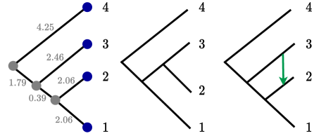
Figure 1: Left: Phylogenetic tree in 4 taxa. Internal (gray) nodes represent speciation events in which an ancestral species differentiates into two. External (blue) nodes, also denoted leaves, represent living species (here denoted 1,2,3,4). Edge weights (in gray) also denoted branch lengths can represent evolutionary time or expected substitutions per site. Center: Different phylogenetic tree on the same 4 taxa in which taxon 2 is grouped with taxon 3 rather than with taxon 1. Nodes are no longer drawn as is the most common representation of phylogenetic trees. Right: Phylogenetic tree with gene flow event depicted as a green arrow. This biological scenario represents the possibility that some genes have the evolutionary history of the phylogenetic tree on the left (with clade $(1,2)$) and some genes, the evolutionary history of the center tree (with clade $(2,3)$).

One of the main challenges when inferring phylogenetic trees is the fact that different genes in the data can have different evolutionary histories due to biological processes such as introgression, hybridization or horizontal gene transfer [33, 12, 28]. An example is depicted in Figure 1 (right) which has one gene flow event drawn as a green arrow. This gene flow event represents the biological scenario in which some genes in taxon 2 get transferred from the lineage of taxon 3, and thus, when reconstructing the evolutionary history of this group of four taxa, some genes will depict the phylogenetic tree that clusters taxa 1 and 2 in a clade (Figure 1 left) and some genes will depict the phylogenetic tree that clusters taxa 2 and 3 in a clade (Figure 1 center). Evolutionary biologists are interested in inferring the correct evolutionary history of the taxon group accounting for the different evolutionary histories of individual genes.

In the absence of gene tree estimation error, the identification of the main trees that represent the evolution of certain gene groups would be trivial. However, estimation error combined with unaccounted biological processes such as incomplete lineage sorting or gene duplications complicate the identification of the main gene evolutionary histories in the data. Thus, novel and scalable tools to accurately classify gene trees into clusters are needed. Surprisingly, unsupervised learning methods have not been explored in phylogenetics. The only implementations of unsupervised learning in phylogenetics aim to cluster DNA sequences [22, 26] or species [7, 27], not trees.

The main challenge to implement unsupervised learning algorithms for phylogenetic trees is the discreteness of tree space. While there exists a proper distance function (Robinson-Foulds distance [30]) in the space of phylogenetic trees that can be used in clustering algorithms [34], the new trend in machine learning is to embed data points into a intelligently selected vector space [36, 35, 13]. Traditionally, there are multiple natural embeddings designed for the space of phylogenetic trees. For example, BHV space [2] is a continuous space for rooted $n$-taxon phylogenetic trees in which each tree is represented as a vector of edge weights in an orthant defined by its topology (bifurcating pattern). While the space is equipped in the geodesic distance, it is not a fully Euclidean space which complicates the embedding, computation of distance, and ultimately, clustering. Other embeddings such as tropical geometric space [24, 19] or the hyperbolic embedding [21, 14] are mathematically sophisticated, yet unnecessarily complicated for standard clustering tasks.

Here, we define a simpler, yet equally powerful, embedding which we denote split-weight which relies on the edge weights of taxon splits to embed a phylogenetic tree into a fully Euclidean vector space. We prove that this embedding preserves phylogenetic similarity and allows us to cluster samples of gene trees into biologically meaningful groups. We implement three standard unsupervised algorithms (K-means, Gaussian mixture model and hierarchical) on the embedding space, and test the performance of our algorithm with simulated and real gene trees. Last, we present a novel open-source Julia package publicly available on GitHub (name and link removed for anonymity) which is easy to use for maximum outreach among the evolutionary biology.

2 Split-Weight Embedding of Phylogenetic Trees

Bipartitions. A bipartition (or split) of the whole set of taxa ($X$) into two groups $X_{1}$ and $X_{2}$ is represented as $X_{1}|X_{2}$ such that $X_{1}\cap X_{2}=\emptyset$ and $X_{1}\cup X_{2}=X$. Let $n=|X|$ denote the total number of taxa in the data. The number of bipartitions is given by $2^{n-1}-1$. For example, for the case of $n=4$ taxa (Figure 1), there are 7 splits (Table 1).

Split-Edge Equivalence. Let $\mathcal{B}_{X}$ be the set of all bipartitions for taxon set $X$ (with cardinality $2^{|X|-1}-1$ as mentioned). Let $T$ be an unrooted phylogenetic tree on taxon set $X$. For every edge $e\in E$ in $T$, there exists a bipartition $b_{e}\in\mathcal{B}_{X}$ such that the removal of $e$ from the tree $T$ results in the two subsets of taxa defined by $b_{e}$. For example, the edge with weight $0.39$ in Figure 1 (left) is an internal edge which, if removed from the tree, would split the taxa into two groups $X_{1}=\{1,2\}$ and $X_{2}=\{3,4\}$, and thus, this edge is uniquely mapped to the bipartition $b_{e}=12|34$. Thus, there is a mapping function $f_{b}:E\rightarrow\mathcal{B}_{X}$ such that $f_{b}(e)$ is the bipartition defined by $e$. We note that not every bipartition is defined by an edge in $T$. For example, the split $13|24$ is not defined by any edge in the tree in Figure 1 (left), and thus, the range of the mapping function $f_{b}(E)\subset\mathcal{B}_{X}$.

Split Representation for Trees. Let $T$ be an unrooted $n$-taxon phylogenetic tree with taxon set $X$. For simplicity, instead of $f_{b}(E)$, we denote by $\mathcal{B}_{T}$ the bipartitions defined by $T$ as the splits $\{f_{b}(e)\}$ defined for every edge $e\in E$ in $T$. For example, the unrooted version of the phylogenetic tree in Figure 1 (left) has five edges that define the bipartitions: $\mathcal{B}_{T}=\{1|234,2|134,12|34,3|124,4|123\}$ in post order traversal. Note that for the unrooted version of this tree, the two children edges of the root are merged into one edge with weight $6.04=1.79+4.25$. In addition, we define a mapping function $f_{w}:\mathcal{B}_{T}\rightarrow\mathbb{(}0,\infty)$ that assigns a numerical value to each bipartition which corresponds to the edge weight of the uniquely mapped edge in the tree. For example, $f_{w}(12|34)=0.39$.

Split-Weight Embedding. Let $T$ be an $n$-taxon unrooted phylogenetic tree on taxon set $X$. Let $\mathcal{B}_{T}$ the bipartitions defined by $T$, and let $\mathcal{B}_{X}$ the set of all bipartitions of $X$. We define the split-weight embedding of $T$ as a ($2^{n-1}-1$)–dimensional numerical vector $y(T)\in\mathbb{[}0,\infty)^{2^{n-1}-1}$ such that the $i$th entry of $y(T)$ corresponds to the $i$th bipartition ($b_{i}$) in $\mathcal{B}_{X}$ with entry value given by:

$$y(T)_{i}=\left\{\begin{array}[]{ll}f_{w}(f_{b}(e))&f_{b}^{-1}(b_{i})=e\in E\\ 0&ow\end{array}\right.,$$

That is, if there is an edge $e\in E$ in $T$ such that $f_{b}(e)=b_{i}$, then the $i$th entry of $y(T)$ is given by the corresponding edge weight $f_{w}(f_{b}(e))$. For example, for 4 taxa, there are 7 bipartitions; five of them correspond to edges in the tree in Figure 1 left (Table 1) and for those, their value in the split-weight embedding vector correspond to the edge weights in $T$. In contrast, the two bipartitions that do not belong to $\mathcal{B}_{T}$ ($13|24$ and $14|23$) have a value in the split-weight embedding vector of $0$, as in [18]. Thus, the split-weight embedding for the unrooted version of the phylogenetic tree $T$ in Figure 1 (left) is the numerical vector $y(T)=(2.06,2.06,2.46,6.04,0.39,0,0)$.

index	bipartition	$y(T)_{i}$
0	1 $\mid$ 2 3 4	2.06
1	2 $\mid$ 1 3 4	2.06
2	3 $\mid$ 1 2 4	2.46
3	4 $\mid$ 1 2 3	6.04
4	1 2 $\mid$ 3 4	0.39
5	1 3 $\mid$ 2 4	0
6	1 4 $\mid$ 2 3	0

Table 1: All possible bipartitions for 4 taxa ($\mathcal{B}_{\{1,2,3,4\}}$) with the numerical entry in the split-weight vector embedding for the unrooted version of the phylogenetic tree $T$ in Figure 1 (left).

3 Clustering Algorithms

For a sample of $n$-taxon unrooted phylogenetic trees $\{T_{1},...,T_{N}\}$, we first embed them into the split-weight numerical vectors: $\{y(T_{1}),...,y(T_{N})\}$. Note that all vectors have the same dimension as all the trees have the same taxon set ($X$). The input matrix ($M\in[0,\infty)^{(2^{n-1}-1)\times N}$) for unsupervised learning algorithms becomes the concatenated embedded vectors. Then, we implement three different types of unsupervised learning methods which are modified to use the input matrix and directly output the predicted labels for each tree in the sample. Figure 2 shows a graphical representation of our unsupervised learning strategy.

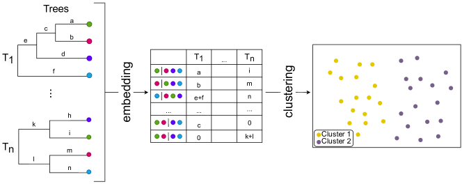
Figure 2: Graphical representation of our unsupervised learning algorithm for phylogenetic trees. In this case, we are embedding 4-taxon trees into a Euclidean space using the split-weight embedding to fit unsupervised learning models. Each point in the scatter plot is a tree. We visualize the clusters with a dimension reduction strategy such as PCA or tSNE.

3.1 K-means

The algorithm [20] is a partitioning method that divides data into K distinct, non-overlapping clusters based on their characteristics, with each cluster represented by the mean (centroid) of its members. It starts by selecting K initial centroids and iterates through two main steps: assigning data points to the nearest centroids, and then updating the position of the centroids to the mean of their assigned points. The algorithm minimizes the squared Euclidean distances within each cluster and ends when the positions of the centroids no longer move.

Instead of traditional K-means, we use Yinyang K-means [8] which has less runtime and memory usage on large datasets. Traditional K-means calculates the distance from all data points to centroids for each iteration. Yinyang K-means uses triangular inequalities to construct and maintain upper and lower bounds on the distances of data points from the centroids, with global and local filtering to minimize unneeded calculations.

The parameters of this algorithm include the number of clusters, the initialization method, and the seed. To select the initial centroids efficiently, we use the K-means++ [1] as default seed algorithm. We also employ the repeating strategy [11] for large datasets to avoid the instability of standard K-means clustering algorithm due to the initial centroid selection. This instability can easily result into convergence to a local minimum, even with the help of a better initial point selection algorithm like K-means++. Therefore, we use a simple strategy of repeating the K-means clustering at least 10 times and retaining the result with the highest accuracy when calculating the accuracy for each large group in our simulations.

3.2 Gaussian mixture model (GMM)

The algorithm [5] is a model-based probabilistic method that assumes data points are generated from a mixture of several Gaussian distributions with unknown parameters. It uses the Expectation Maximization (EM) algorithm to update the parameters iteratively in order to optimize the log-likelihood of the data until convergence. It is similar yet more flexible than K-means as it allows for mixed membership.

The parameters of this model include the number of clusters, the initialization method, and the covariance type. We use K-means as the method for selecting initial centrals and choose diagonal covariance as covariance type. We also employ repeating K-means [11] to find the best starting centers.

3.3 Hierarchical clustering

The algorithm is a hierarchical method that creates a clustering tree called a dendrogram. Each leaf on the tree is a data point, and branches represent the joining of clusters. We can ’cut’ the tree at different heights to get a different number of clusters. This method does not require the number of clusters to be specified in advance and can be either agglomerative (bottom-up) or divisive (top-down). The parameters of this model are the linkage method, and the number of cluster. As default, we use Ward’s method [37] as linkage method for hierarchical clustering.

4 Simulation study

We perform simulation tests of K-means, GMM, and hierarchical clustering with K = 2 for samples of $N$ trees, each with $n$ taxa where we vary $N$ and $n$ as described below. For each combination of $n$ and $N$, we generate 100 datasets to account for performance variability. Tree variability is simulated with the PhyloCoalSimulations Julia package [10] which takes a species tree as input and simulates gene trees under the coalescent model [29] which generates tree variability due to random sorting of lineages within populations. In this sense, we expect simulated trees to cluster around the chosen species tree. The level of expected variability in the sample of gene trees is governed by the edge weights in the species tree (longer branches resulting in less tree variability) [6]. All trees are embedded into the split-weight space, and the vectors are standarized prior to clustering. Visualization of clusters is performed via PCA.

To quantify the performance of unsupervised learning models, we use the Hungarian algorithm [25] to find the grouping method with the largest overlap between predicted and true labels. In this grouping method, the fact that the predicted label is different from the true label means that the tree is not classified into the correct group. Therefore, the accuracy is defined as $\frac{2N-t}{2N}$ where $t$ is the number of trees with different predicted and true labels.

4.1 Clustering of trees with different topologies

For $n=4$ taxa, there are 15 possible bifurcating patterns (tree topologies). For each of the 15 4-taxon species trees, we simulated samples of $N=50,100,500,1000,5000$ trees with PhyloCoalSimulations [10] for two choices of edge weights in the species trees: 1) all edge weights set to $1.0$ coalescent unit, or 2) each edge weight randomly selected from an uniform distribution $(0.5,2)$ coalescent units. The rationale is that $1.0$ coalescent unit generates medium levels of gene tree discordance [6], and thus, we expect the clustering algorithms to perform accurately, whereas shorter branches (e.g. $0.5$ coalescent units) produce more tree heterogeneity further complicating clustering.

Figure 3 (left) shows a heatmap of the prediction accuracy of the different clustering algorithms. Each cell in the heatmap represents a comparison between the row and column tree (only rows labeled, but the order of the columns is the same). Trees are ordered depending of their unrooted topology. For example, the first 5 rows (and columns) correspond to the 5 different rooted versions of the unrooted tree corresponding to the split $12|34$; the next 5 rows (and columns) to the split $13|24$, and the last 5 rows (and columns) to the split $14|23$. The darker the color, the more accurate the classification of the two trees. We can see a diagonal block pattern in the heatmaps which illustrates the difficulty of separating two clusters defined by two rooted trees with the same unrooted representation. The heatmaps are arranged by clustering algorithm (three columns: K-means, GMM and hierarchical) and number of trees in the sample ($N=50$ and $N=5000$). Similar plot for $N=100,500,1000$ can be found in the Appendix. We can see that the accuracy of K-means is robust to sample size, while the accuracy of GMM is higher for larger number of trees ($N=5000$). Hierarchical clustering shows the worst performance of the three methods.

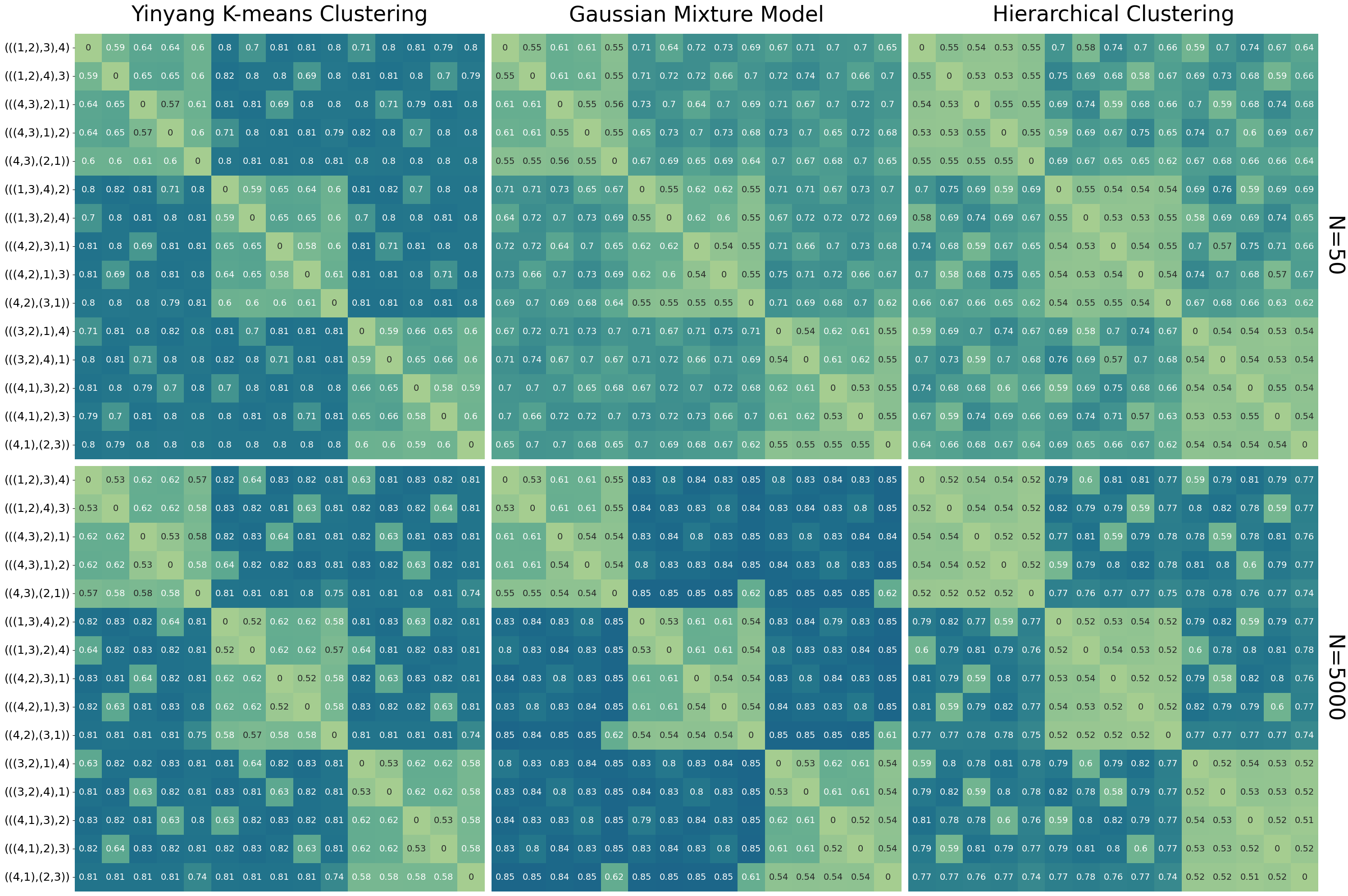
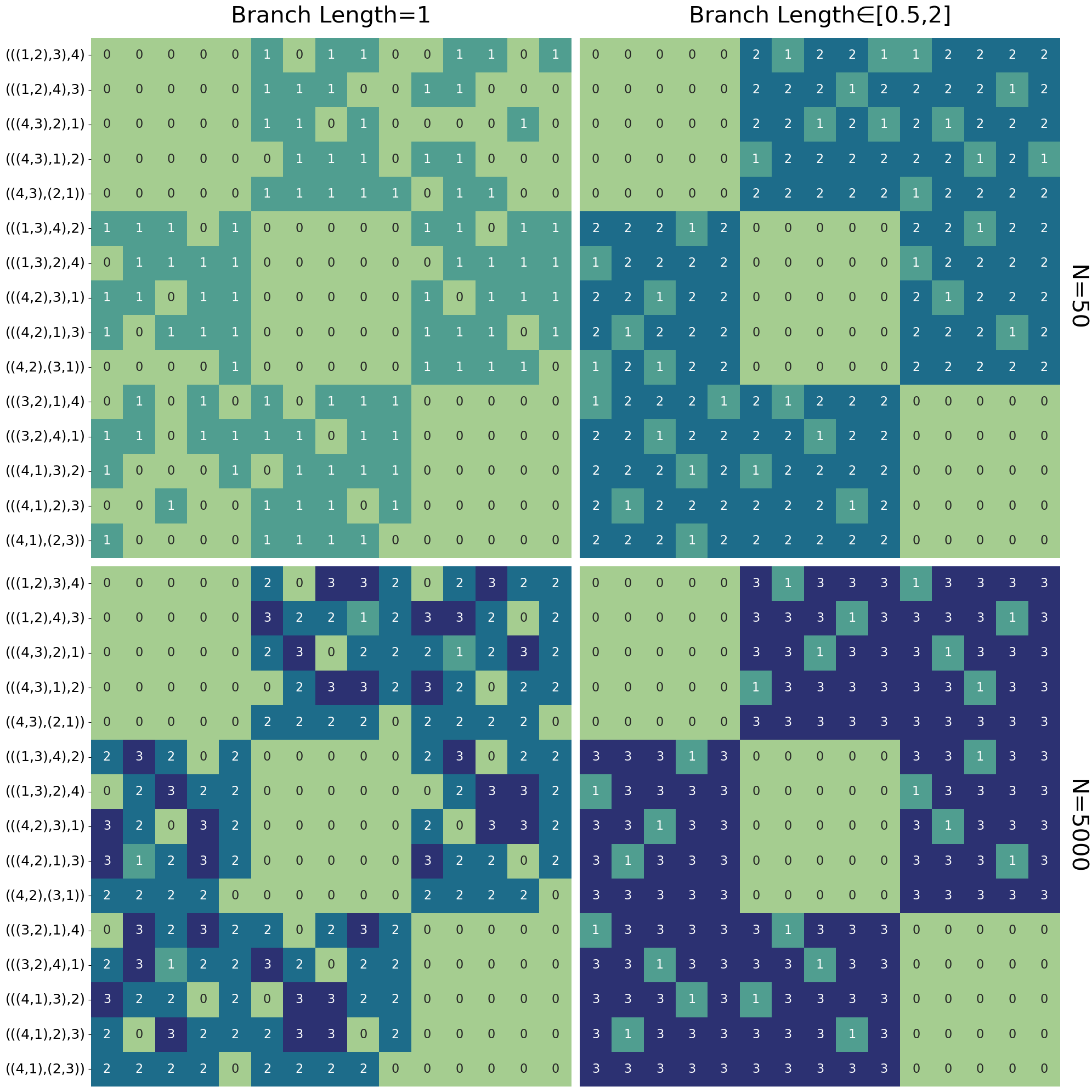
Figure 3: Left: Heatmaps of classificacion accuracy on the 15 trees with 4 taxa. Each panel corresponds to the classification accuracy of pairwise comparisons for two clusters originated on two trees (row and column) for one clustering method (columns: K-means, GMM and Hierarchical) and one sample size (rows: $N=50$ and $N=5000$). Within each panel, trees are sorted based on their unrooted topology (first 5 rows correspond to split $12|34$; next 5 to the split $13|24$, and last 5 to the split $14|23$). Off-diagonal blocks (trees with different unrooted representation) can be accurately separated as different clusters by GMM with large sample size ($N=5000$), and by K-means for any sample size. Right: Heatmaps on the number of algorithms that reach $80$% classification accuracy ($0,1,2,$ or $3$ algorithms) by edge weight strategy (columns: edge weights equal to $1$ or edge weights randomly chosen in $(0.5,2)$) and sample size (rows: $N=50,5000$).

Figure 3 (right) shows a different type of heatmap in which we summarize the performance of all three methods. Each cell in the heatmap can have four values: $0$ if none of the three methods have a classification accuracy above $80$%; $1$ if one of the three methods has a classification accuracy above $80$%; $2$ if two of the three methods have a classification accuracy above $80$%, and $3$ if all three methods have a classification accuracy above $80$%. The two columns correspond to the strategy to set edge weights (all edge weights equal to $1.0$ in the left column and edge weights randomly selected in $(0.5,2)$ in the right column). Unlike standard phylogenetic methods that tend to perform better when edges are $1.0$ coalescent unit long, the clustering methods here tested perform better with variable edge weights. Furthermore, we can see that with larger sample sizes ($N=5000$), most methods are able to distinguish samples originated from trees that do not have the same unrooted topology (off-diagonal blocks).

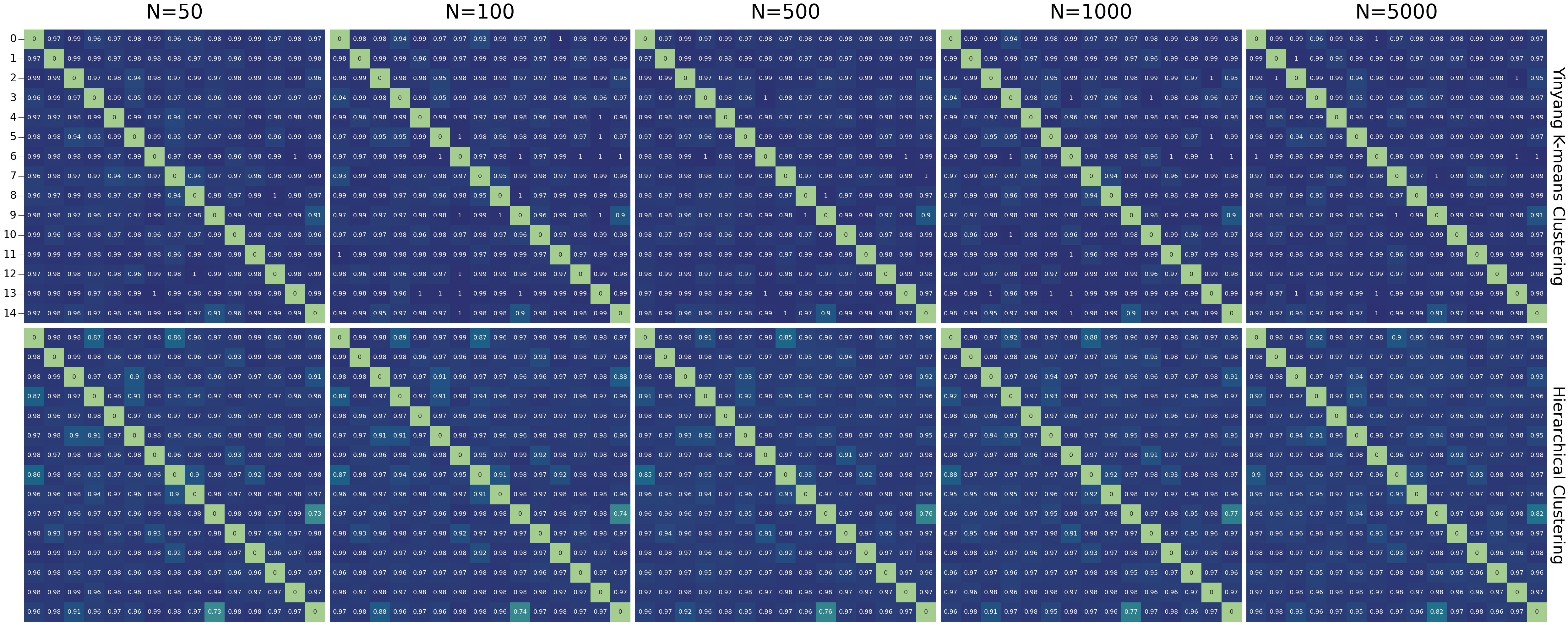
Figure 8: Heatmaps of classificacion accuracy on the 15 randomly generated trees with 8 taxa. Each panel corresponds to the classification accuracy of pairwise comparisons for two clusters originated on two trees (row and column) for one clustering method (rows: K-means and Hierarchical) and one sample size (columns: $N=50,100,500,1000,5000$).

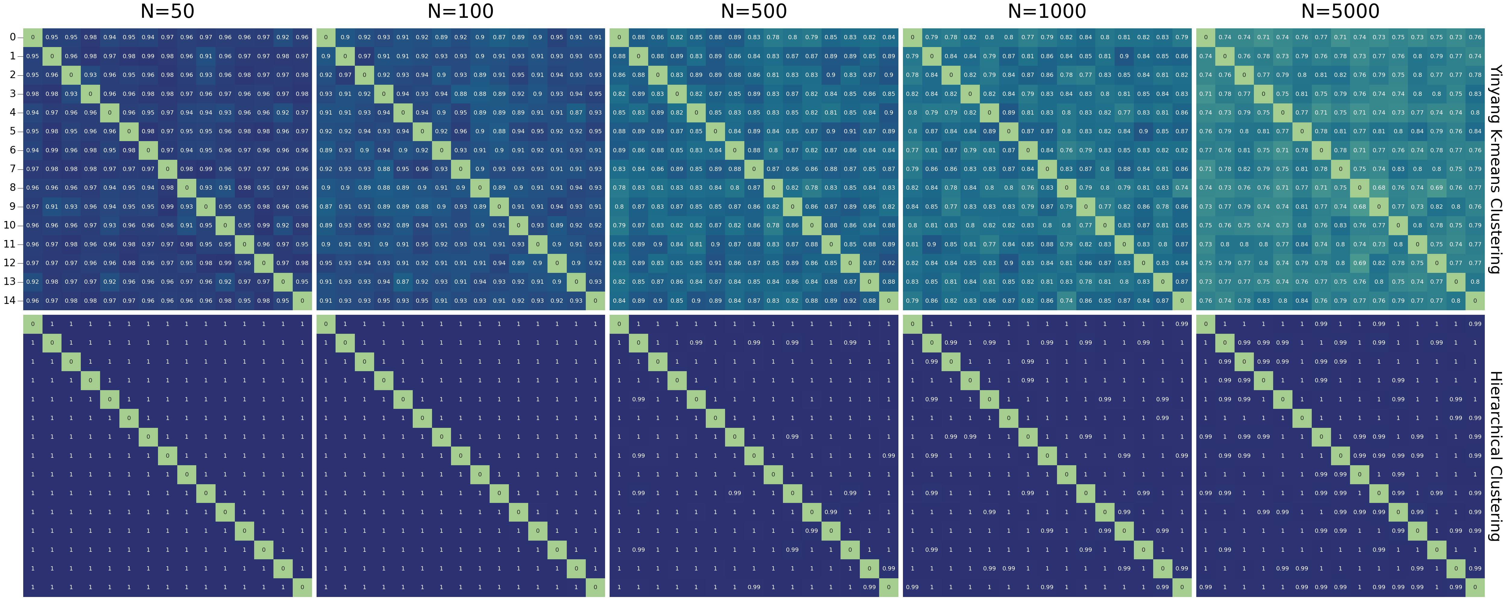
Figure 9: Heatmaps of classificacion accuracy on the 15 randomly generated trees with 16 taxa. Each panel corresponds to the classification accuracy of pairwise comparisons for two clusters originated on two trees (row and column) for one clustering method (rows: K-means and Hierarchical) and one sample size (columns: $N=50,100,500,1000,5000$).

For the case of more than 4 taxa, we cannot list all of the tree topologies (10,395 total unrooted trees for 8 taxa and 213,458,046,676,875 total unrooted trees for 16 taxa), so we randomly generate 15 8-taxon trees and 15 16-taxon trees using the simulating algorithm in the R package SiPhyNetwork [15] under a birth-death model. We focus on the case of edge weights randomly chosen uniformly in the interval $(0.5,2)$. Figures 8 and 9 in the Appendix show the classification of all methods to cluster samples of trees accurately. As classification appears to be easy for randomly selected trees, we design another simulation study to compare the accuracy on trees that are more similar to each other (next section).

4.2 Clustering of trees in NNI-neighborhoods

The Nearest Neighbor Interchange (NNI) move is a type of phylogenetic tree arrangement that selects an internal branch of a given tree and then swaps adjacent subtrees across that branch. It generates alternative tree topologies that are “nearest neighbours” to the original tree, differing only in the local arrangement of the subtrees connected by the chosen branch. For a given tree, we can define a NNI-neighborhood as all the trees that are one NNI move away from the selected tree (or any number of NNI moves away). In this section, we test whether the clustering algorithms are accurate enough to distinguish trees within the same NNI-neighborhood.

Using the simulating algorithm in the R package SiPhyNetwork [15] under a birth-death model, we randomly generate one 8-taxon tree and one 16-taxon tree, and then we perform 1, 2, 3, 4 and 5 NNI moves on each tree to produce 10 new trees (5 with 8 taxa and 5 with 16 taxa). The NNI function for phylogenetic trees is implemented in PhyloNetworks [32]. The edge weights are randomly selected from an uniform distribution $(0.5,2)$ coalescent units. For each of the trees, we simulate samples of $N=50,100,500,1000,5000$ trees with PhyloCoalSimulations [10].

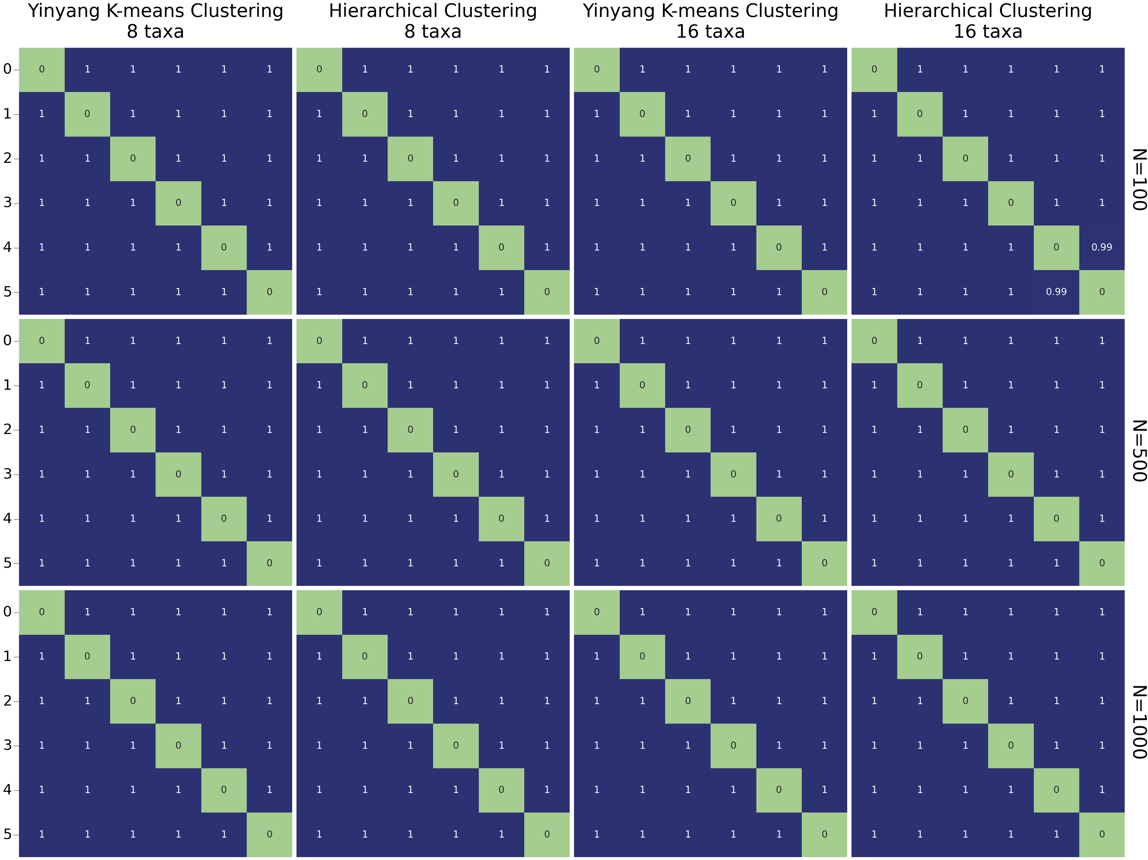
Figure 10: Heatmaps of classification accuracy on one randomly generated tree with 8 taxa (first two columns) or 16 taxa (second two columns) with 5 other trees obtained by $1,2,3,4$ or $5$ NNI moves on the original tree. Rows correspond to sample size ($N=100,500,1000$). Classificacion accuracy is high for both methods even for very similar trees (1 NNI move away, for example).

Figure 4 shows the classification accuracy of trees with 8 and 16 taxa, and their corresponding neighbor trees obtained by performing $1,2,3,4$ or $5$ NNI moves on the original tree. Despite the similarity of the trees under comparison, the methods are able to classify quite accurately clusters of trees originated from two similar trees. This implies that the split-weight embedding is able to preserve the necessary signal to classify phylogenetic trees even for closely related clusters. Figure 10 in the Appendix shows the same figure for $N=100,500,1000$ trees.

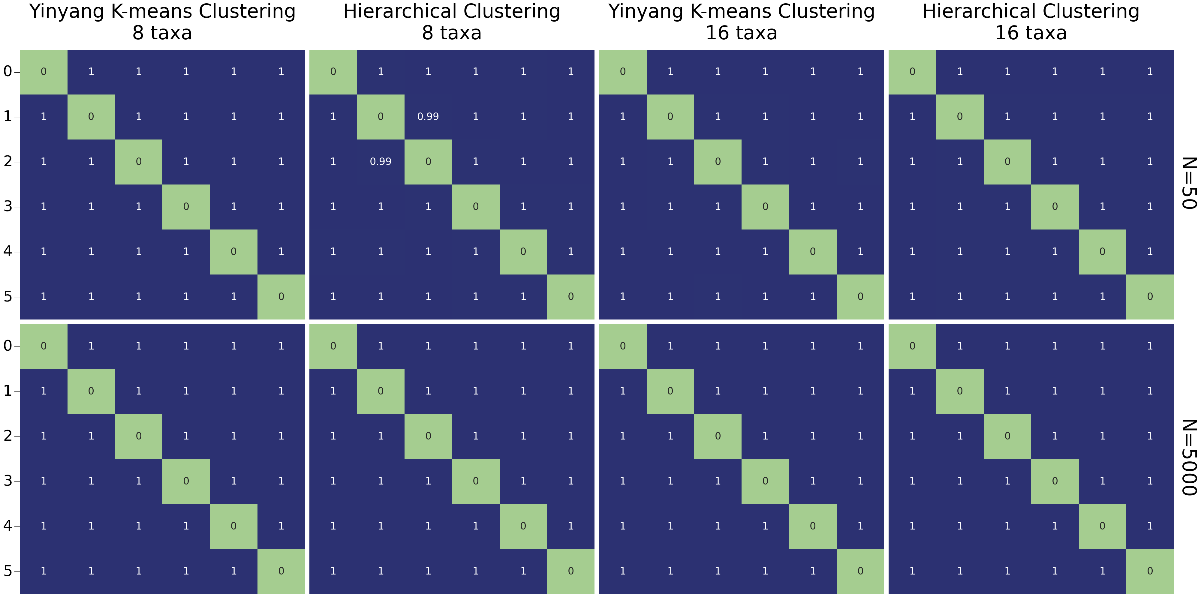
Figure 4: Heatmaps of classification accuracy on one randomly generated tree with 8 taxa (first two columns) or 16 taxa (second two columns) with 5 other trees obtained by $1,2,3,4$ or $5$ NNI moves on the original tree. Rows correspond to sample size ($N=50$ trees on top, and $N=5000$ trees on bottom). Classificacion accuracy is high for both methods even for very similar trees (1 NNI move away, for example) which illustrates the preservation of phylogenetic signal by the split-weight embedding.

4.3 Clustering of trees with the same topology, but different edge weights

To test the performance of the clustering algorithms to classify trees that have the same topologies, but different edge weights, we simulate trees under the same species tree topology with six different sets of edge weights: 1) all edge weights equal to $1$ (denoted org in the figures); 2) all edge weights lengths equal to $1.5$ (denoted inc in the figures); 3) randomly selected edge weights uniformly in $(1,2)$ (denoted inc_r in the figures); 4) all branch lengths equal to $0.5$ (denoted dec in the figures); 5) randomly selected edge weights uniformly in $(0,1)$ (denoted dec_r in the figures), and 6) randomly selected edge weights uniformly in $(0,2)$ (denoted all_r in the figures). We only focus on the 4-taxon tree topologies for these tests. For each of the trees, we simulated samples of $N=50,100,500,1000,5000$ trees with PhyloCoalSimulations [10].

While we showed that GMM can accurately identify tree clusters defined by different topologies (Figure 3), it appears that this algorithm does not have enough sensitivity to identify clusters originated from the same tree topology (Figure 5). K-means, on the other hand, is able to identify such clusters as long as the edge weights are sufficiently different (dec vs inc, for example). Figures for other tree topologies are in the Appendix with similar conclusion.

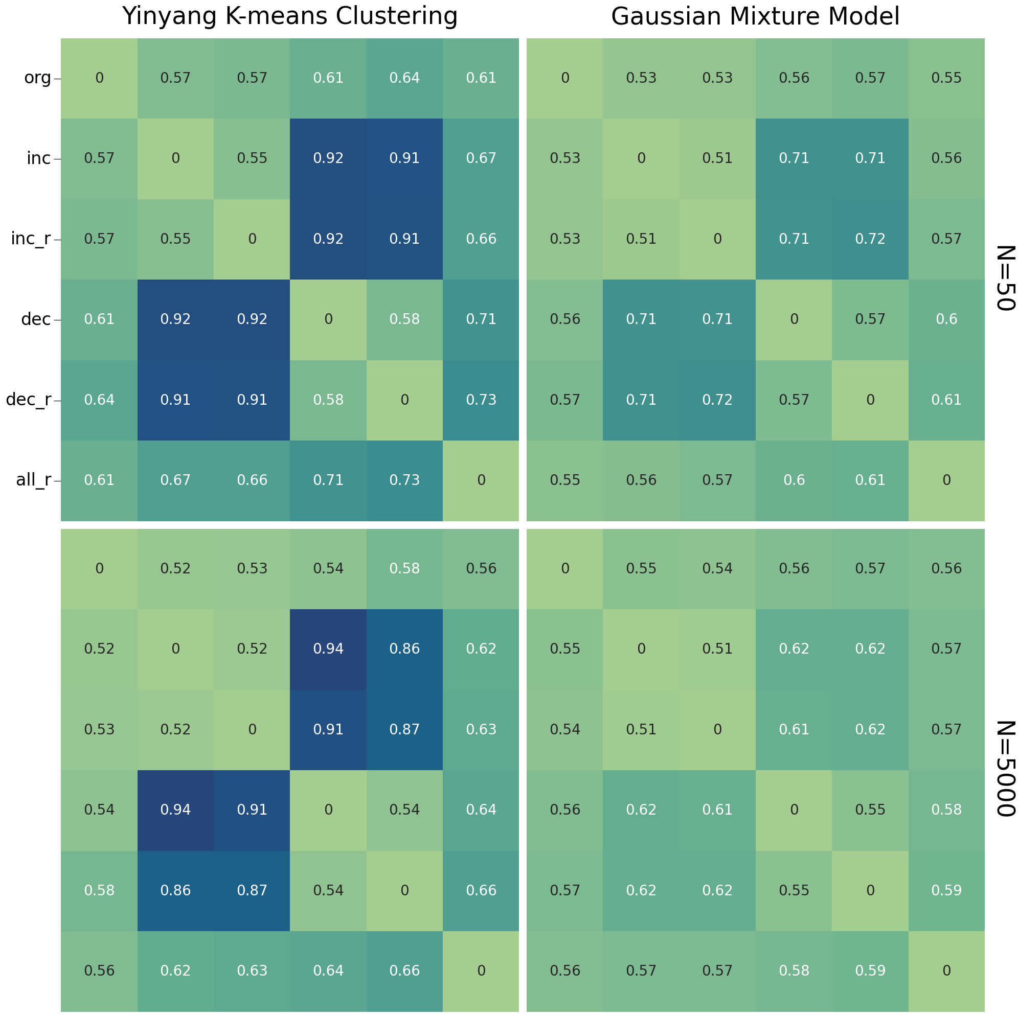
Figure 5: Heatmaps of classification accuracy on 4-taxon tree $(((4,3),2),1)$ by the two methods (columns: K-means and GMM) and sample size (rows: $N=50$, $N=5000$) by different set of edge weights. Clusters defined by the same tree topology can be accurately identified by K-means if edge weights are sufficiently different (inc vs dec, for example), but not by GMM.

5 Reticulate evolution in baobabs

In-frame codon alignments of baobab target-enrichment data [17] are used to estimate gene trees under maximum likelihood (ML) [9] with IQTREE v.2.1.3 and default settings [23]. The ML analyses treats alignments as nucleotide data and the best model is determined by ModelFinderPlus [16], which uses the Bayesian Information Criterion for model selection.

The data then consist of 371 estimated trees in 8 species of Adansonia: A. digitata (continental Africa), A. gregorii (Australia), A. grandidieri (Madagascar), A. suarezensis (Madagascar), A. madagascariensis (Madagascar), A. perrieri (Madagascar), A. za (Madagascar), and A. rubrostipa (Madagascar). The data also contain an outgroup Scleronema micranthaum, so in total, there are 9 taxa. We remove 4 trees that only had 8 taxa, and 5 outlier trees with pathologically long edges so that the final dataset contain 363 trees which we embed in the split-weight space. We standarize the resulting matrix as in the simulation study, and cluster the vectors using the K-means algorithm ($K=2$). After clustering, we use Densitree [3] to identify the consensus tree of each cluster via the root canal method.

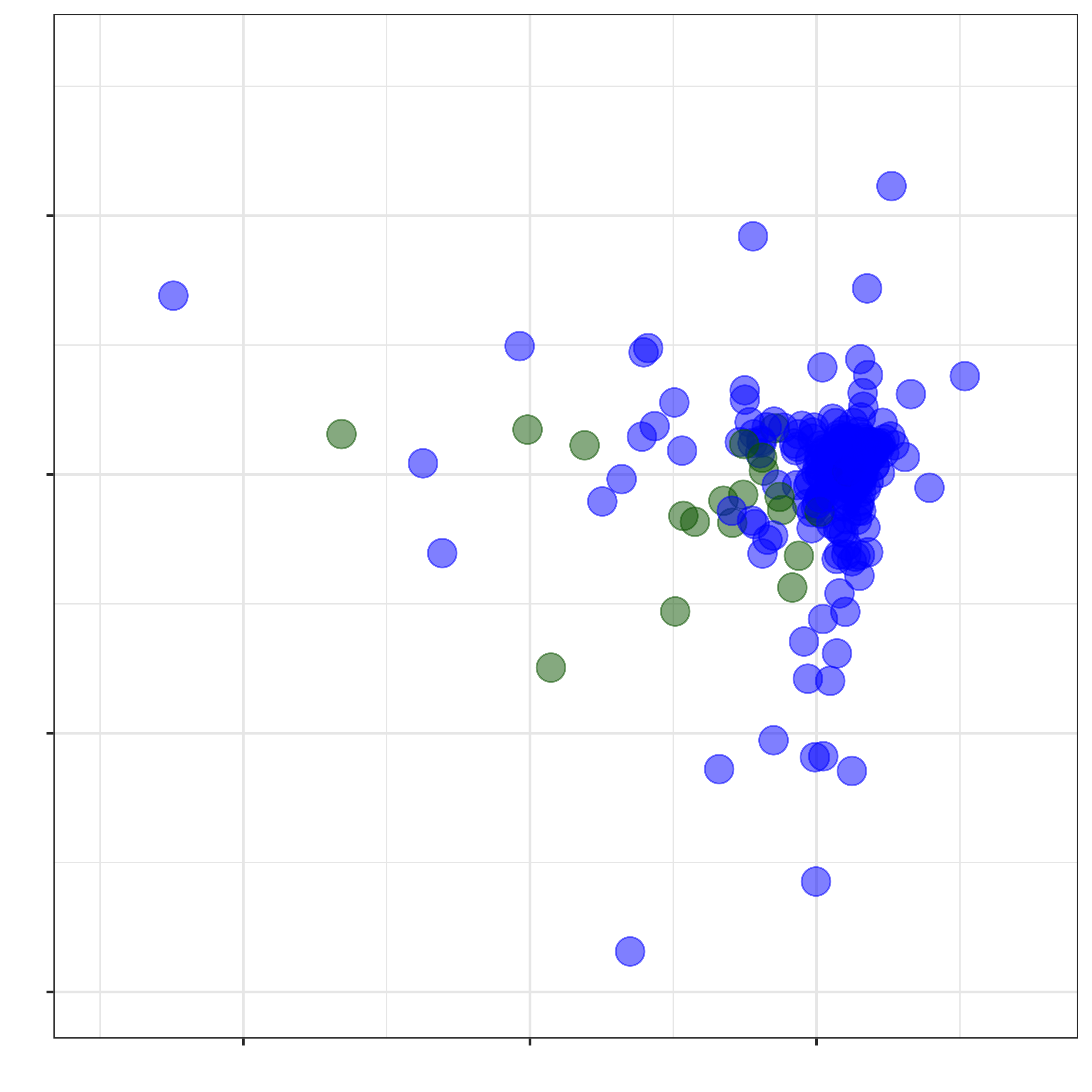
Figure 13: PCA plot for the clustering of baobabs phylogenetic trees (center). The two clusters (blue and green) are highly imbalanced (341/363 vs 22/363), but these partition agrees with the evolutionary history of the group (Figure 6 in the main text) which involves one gene flow event for $11.2$% of the genes [17]. Left and right trees represent the consensus tree created by Densitree [3] for each cluster.

The two resulting clusters are not balanced: 341 trees in cluster 1 and 22 trees in cluster 2 (Figure 13 in th Appendix). This is expected given the evolutionary history of the baobabs group (Figure 6 left). The original publication [17] identified one reticulation event (blue arrow) representing $11.8$% gene flow. This means that we expect $11.8$% of the genes to follow the blue arrow back to the root in their evolutionary history, and thus, most of the genes ($88.2$%) will have a tree that puts clade ((A.mad, A.ped), A.zaa) sister to (A.gra, A.sua) (Figure 6 center; clade highlighted in blue) whereas a few genes ($11.8$%) will place ((A.mad, A.ped), A.zaa) sister to A.rub (Figure 6 right; clade highlighted in green).

The accurate identification of the consensus trees for each cluster, in spite of estimation error and other biological processes in addition to reticulation, is an important result for phylogenetic inference. Estimating a phylogenetic network with 9 taxa (tree plus gene flow event in Figure 6 left) could take up to two days of compute time depending on the method used [31]. Clustering the input trees, building the consensus trees and reconstruct the network from the consensus trees cannot take more than a few minutes. Our work shows the promise of machine learning (unsupervised learning specifically) to aid in the estimation of phylogenetic trees and networks in a scalable manner.

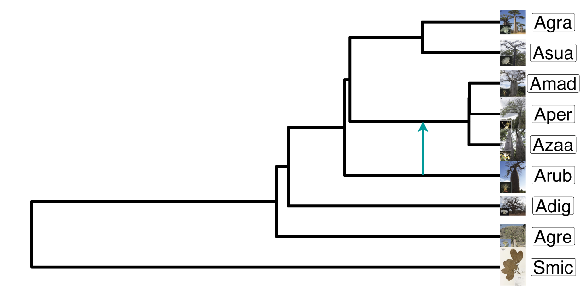
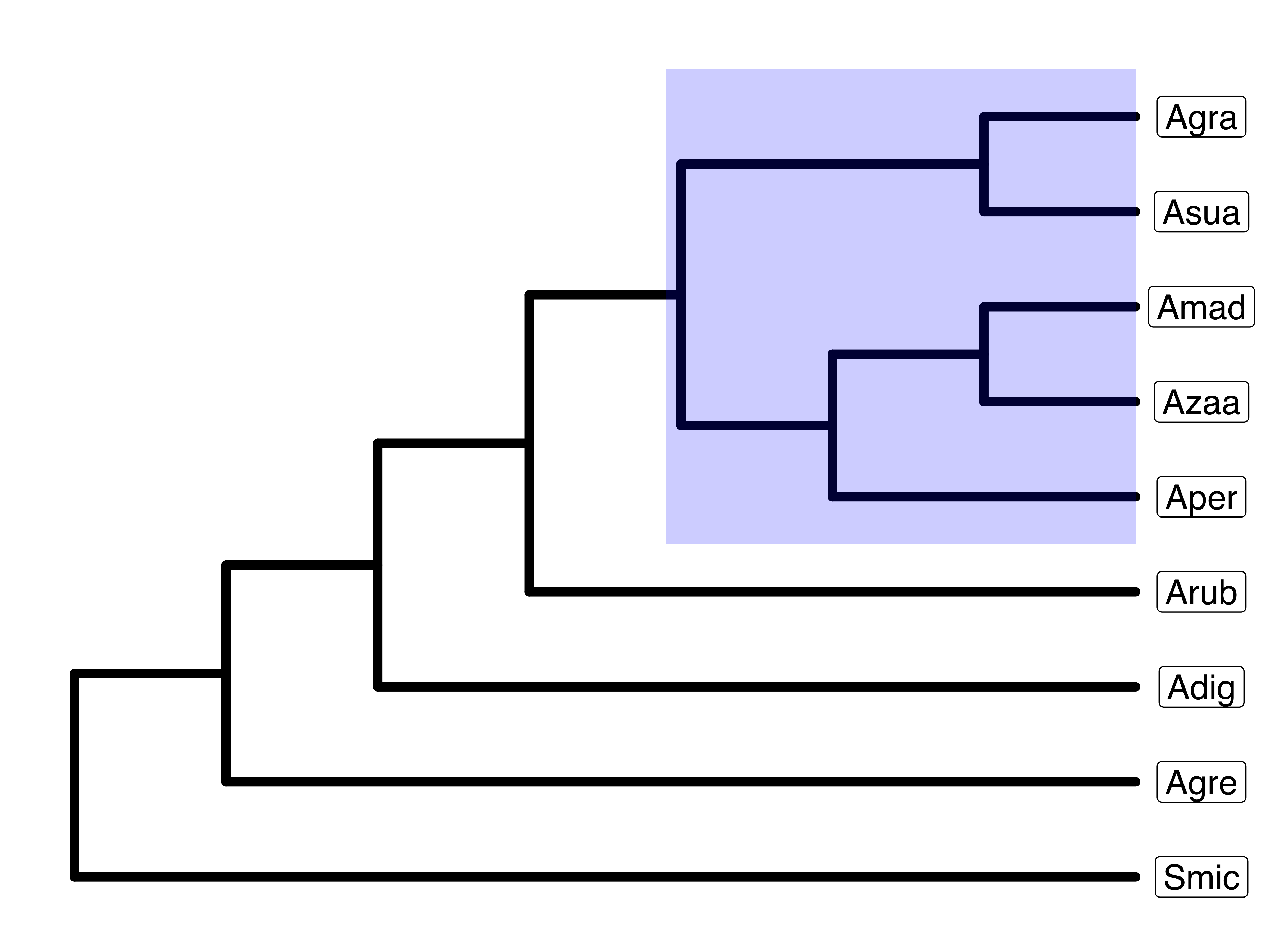
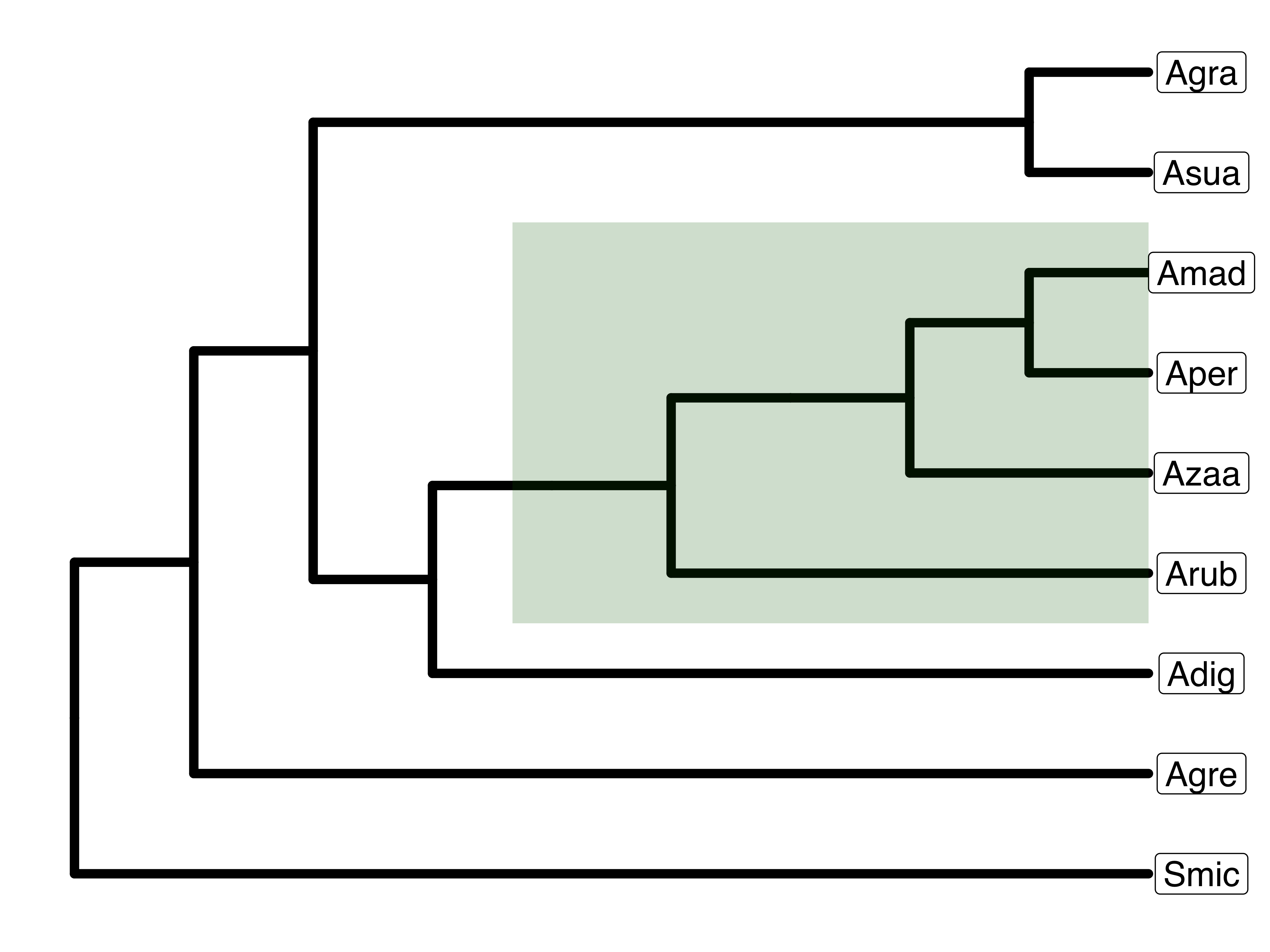
Figure 6: Clustering via split-weight embedding recovers the correct evolutionary relationship in baobabs. Estimated gene trees from the baobabs group cluster around two consensus trees (341/363 genes around the center tree and 22/363 genes around the right tree) that represent the two correct possibilities created by the gene flow event in the phylogenetic network for the group (left) as estimated by the original study [17]. The placement of the (A.mad, A.per, A.zaa) clade changes from being sister to clade (A.gra, A.sua) in the center tree (clade highlighted in blue) to be sister of taxon A.rub in the right tree (clade highlighted in green).

6 Discussion

Here, we apply the first (to our knowledge) implementation of unsupervised learning in the space of phylogenetic trees via the novel and powerful split-weight embedding. Via extensive simulations, we show that the split-weight embedding is able to capture meaningful evolutionary relationships while keeping the simplicity of a standard Euclidean space. Our implementation is able to cluster trees with different topologies, and even trees with the same topology, but different edge weights. As usual in machine learning applications, the larger the sample size (number of trees), the more accurately the different clusters were recovered. On average, K-means was the desired choice of algorithm as it showed robust performance across sample size and number of taxa, yet for large trees (8 or 16 taxa), hierarchical clustering outperforms K-means in terms of running efficiency and accuracy. For the case of 4 taxa, GMM outperforms K-means when the sample size increased.

The bottleneck of our implementation is the curse of dimensionality. In its current version, we do not perform dimension reduction except for visualization purposes. The dimension of the split-weight embedded vector is given by the number of bipartitions which is $2^{n-1}-1$ for $n$ taxa. In addition, the embedded vector is highly sparse. For a tree of $n$ taxa, there are $2n-3$ edges, and thus, only $2n-3$ entries of the embedded vector will be different than zero. So, for example, for $n=8$ taxa, the embedded vector is 127-dimensional with 13 non-zero entries; for $n=16$ taxa, the embedded vector is 32767-dimensional with 29 non-zero entries. The field of phylogenetic trees deals with datasets of hundreds or thousands of taxa consistently. Future work will involve the study of dimension reduction techniques, as well as compression, such as autoencoder models in order to improve the scalability and stability of our algorithms.

Future work will also involve the comparison of different tree embeddings in terms of evolutionary signal. Here, we tested the embedding’s ability to accurately cluster trees into meaningful groups, yet the embedded vectors could be used to calculate pairwise taxon distances and build distance-based trees such as neighbor-joining. Different embeddings could retain better phylogenetic signal, and thus, could be preferred when the goal is to reconstruct a phylogenetic tree accounting for gene tree discordance.

Finally, here we utilize Densitree [3] to obtain a representation of the consensus tree per cluster. We can, however, explore similar ideas to those in BHV space regarding the computation Fréchet sample means and Fréchet sample variances [4] which could set the foundation of classical statistical theory on the split-weight embedding space.

7 Data and code availability

The baobabs dataset was made publicly available by the original publication [17] and can be accessed through the Dryad Digital Repository http://doi.org/10.5061/dryad.mf1pp3r. The split-weight embedding and unsupervised learning algorithms are implemented in the open source publicly available Julia package available in the GitHub repositoryhttps://github.com/solislemuslab/PhyloClustering.jl. All the simulation and real data scripts for our work are available in the public GitHub repository https://github.com/YiboK/PhyloClustering-scripts.

8 Acknowledgements

This work was supported by the National Science Foundation [DEB-2144367 to CSL]. The authors thank Marianne Björner and Reed Nelson for help with setting up tests, and Zhaoxing Wu for providing the testing data.

Appendix A Supplementary Figures

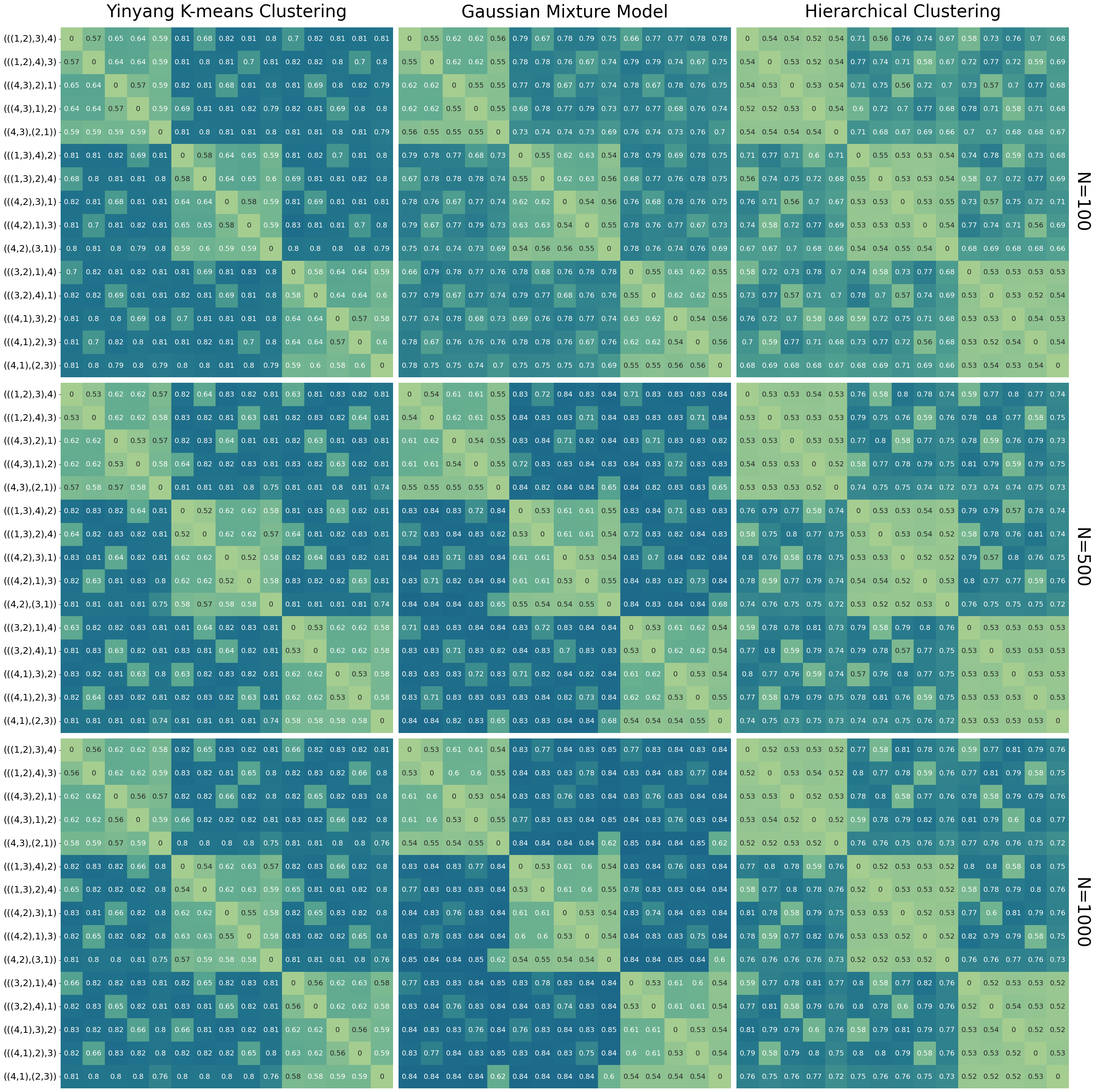
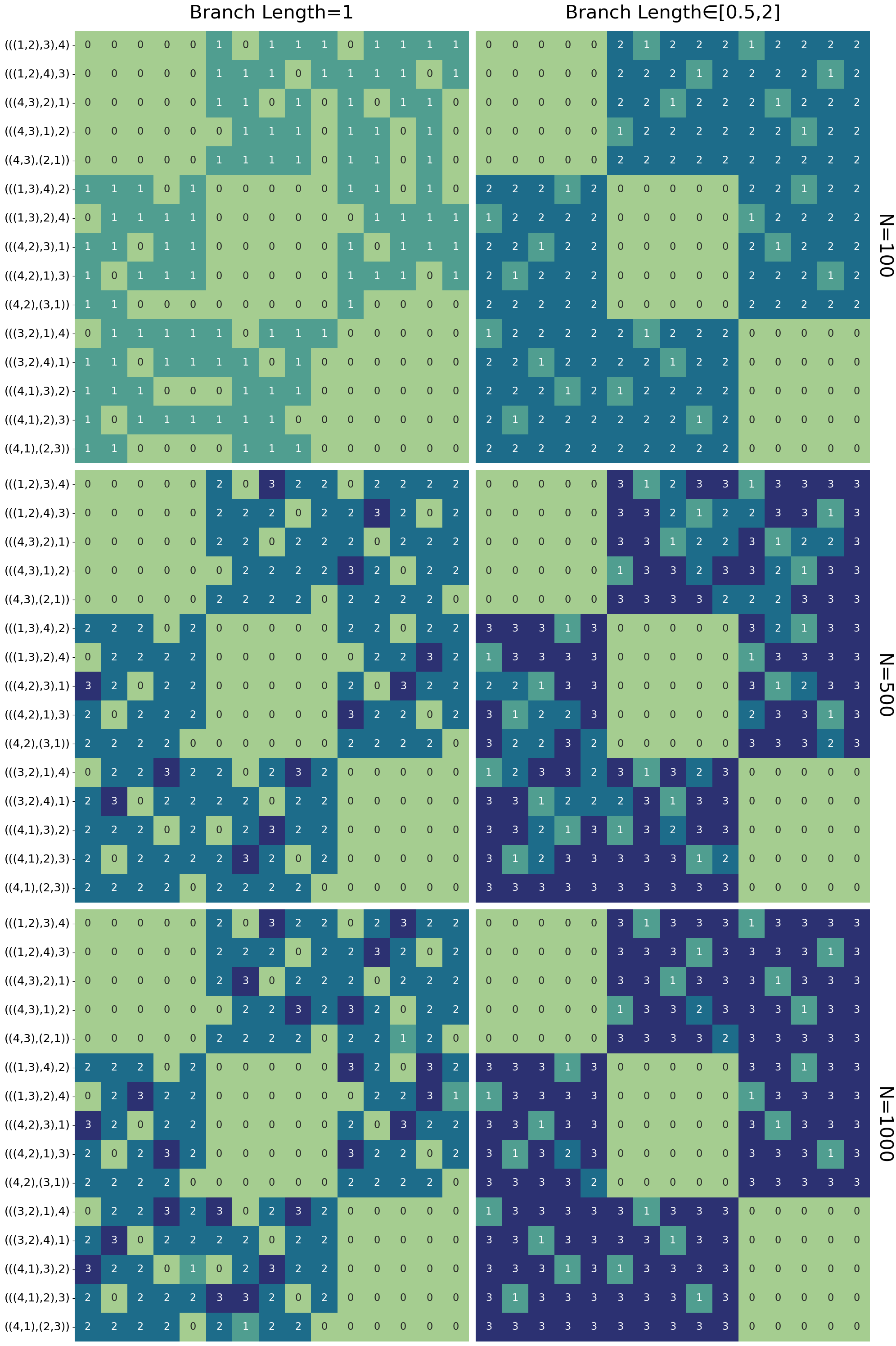
Figure 7: Left: Heatmaps of classificacion accuracy on the 15 trees with 4 taxa. Each panel corresponds to the classification accuracy of pairwise comparisons for two clusters originated on two trees (row and column) for one clustering method (columns: K-means, GMM and Hierarchical) and one sample size (rows: $N=100,500,1000$). Within each panel, trees are sorted based on their unrooted topology (first 5 rows correspond to split $12|34$; next 5 to the split $13|24$, and last 5 to the split $14|23$). Right: Heatmaps on the number of algorithms that reach $80$% classification accuracy ($0,1,2,$ or $3$ algorithms) on edge weight strategy (columns: edge weights equal to $1$ or edge weights randomly chosen in $(0.5,2)$) and sample size (rows: $N=100,500,1000$).

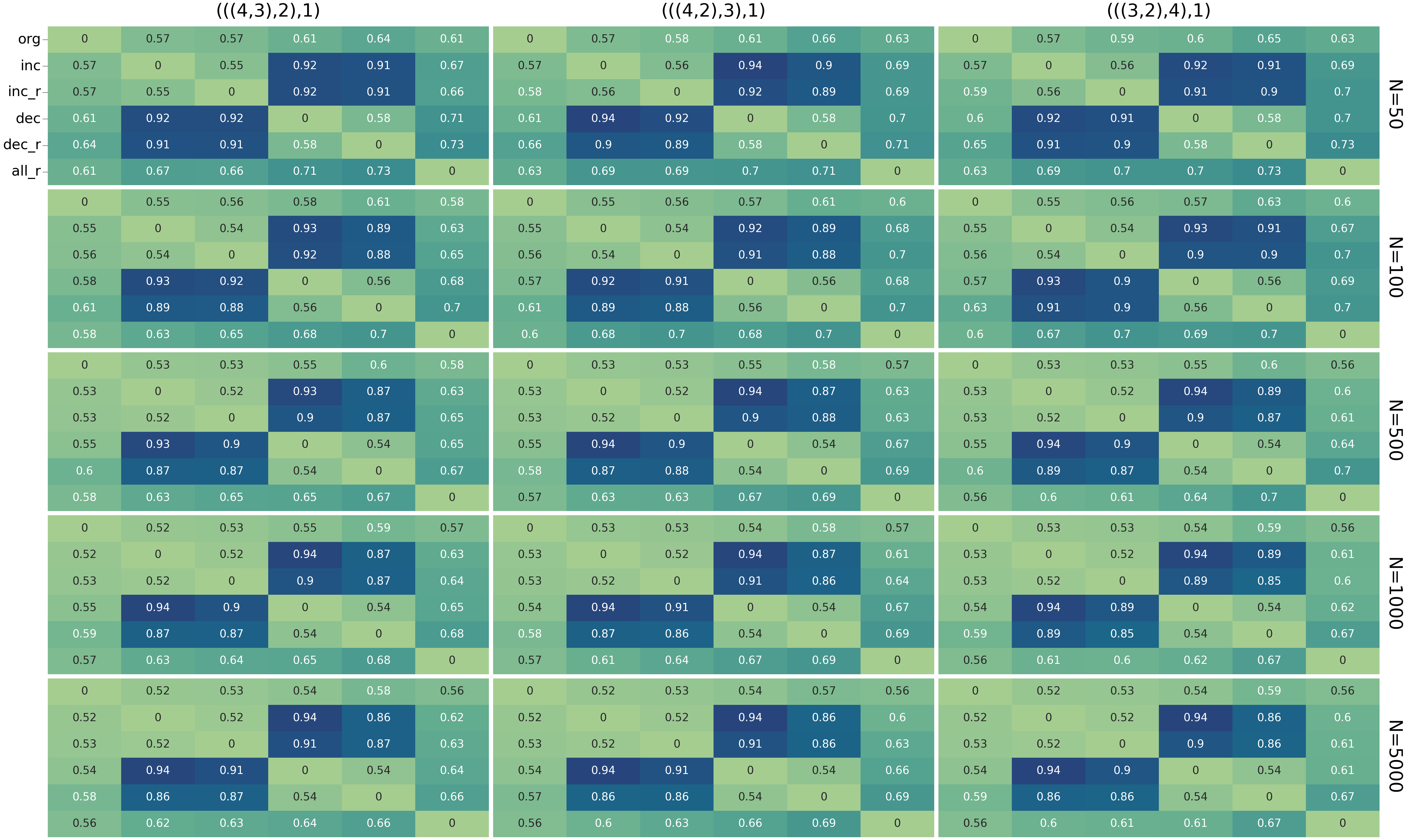
Figure 11: Heatmaps of K-means classification accuracy on three 4-taxon trees (columns) by sample size (rows: $N=50,100,500,1000,5000$) by different set of edge weights. Clusters defined by the same tree topology can be accurately identified if edge weights are sufficiently different (inc vs dec, for example).

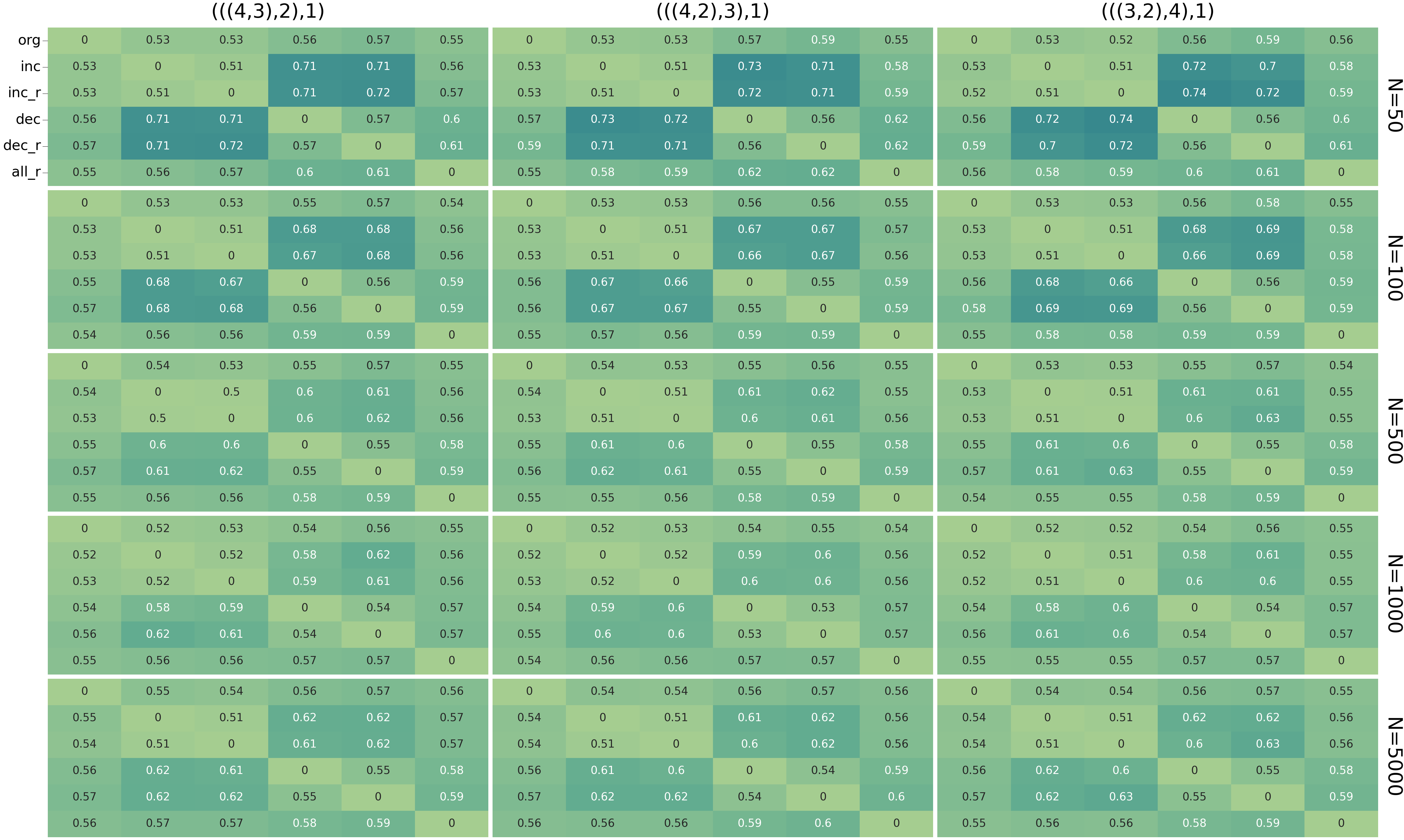
Figure 12: Heatmaps of GMM classification accuracy on three 4-taxon trees (columns) by sample size (rows: $N=50,100,500,1000,5000$) by different set of edge weights. Clusters defined by the same tree topology cannot be accurately identified compared to using K-means (Figure 11).

References

- [1] David Arthur and Sergei Vassilvitskii. K-means++: The advantages of careful seeding. In Proceedings of the Eighteenth Annual ACM-SIAM Symposium on Discrete Algorithms, SODA ’07, page 1027–1035, USA, 2007. Society for Industrial and Applied Mathematics.
- [2] Louis J Billera, Susan P Holmes, and Karen Vogtmann. Geometry of the space of phylogenetic trees. Advances in Applied Mathematics, 27(4):733–767, 2001.
- [3] Remco R. Bouckaert. DensiTree: Making sense of sets of phylogenetic trees. Bioinformatics, 26(10):1372–1373, 03 2010.
- [4] Daniel G Brown and Megan Owen. Mean and variance of phylogenetic trees. Systematic biology, 69(1):139–154, 2020.
- [5] Lars Buitinck, Gilles Louppe, Mathieu Blondel, Fabian Pedregosa, Andreas Mueller, Olivier Grisel, Vlad Niculae, Peter Prettenhofer, Alexandre Gramfort, Jaques Grobler, Robert Layton, Jake Vanderplas, Arnaud Joly, Brian Holt, and Gaël Varoquaux. API design for machine learning software: experiences from the scikit-learn project. arXiv, 1(1309.0238), 2013.
- [6] James H Degnan and Noah A Rosenberg. Gene tree discordance, phylogenetic inference and the multispecies coalescent. Trends in ecology & evolution, 24(6):332–340, 2009.
- [7] Shahan Derkarabetian, Stephanie Castillo, Peter K Koo, Sergey Ovchinnikov, and Marshal Hedin. A demonstration of unsupervised machine learning in species delimitation. Molecular phylogenetics and evolution, 139:106562, 2019.
- [8] Yufei Ding, Yue Zhao, Xipeng Shen, Madanlal Musuvathi, Todd Mytkowicz, and Madan Musuvathi. Yinyang k-means: A drop-in replacement of the classic k-means with consistent speedup. In Proceedings of the 32nd International Conference on Machine Learning, ICML 2015, pages 579–587, 7 2015.
- [9] Joseph Felsenstein. Evolutionary trees from dna sequences: a maximum likelihood approach. Journal of molecular evolution, 17:368–376, 1981.
- [10] John Fogg, Elizabeth S Allman, and Cécile Ané. Phylocoalsimulations: A simulator for network multispecies coalescent models, including a new extension for the inheritance of gene flow. Systematic Biology, page syad030, 2023.
- [11] Pasi Fränti and Sami Sieranoja. How much can k-means be improved by using better initialization and repeats? Pattern Recognition, 93:95–112, 2019.
- [12] Mark S. Hibbins and Matthew W. Hahn. The effects of introgression across thousands of quantitative traits revealed by gene expression in wild tomatoes. PLOS Genetics, 17(11):1–20, 11 2021.
- [13] Yanrong Ji, Zhihan Zhou, Han Liu, and Ramana V Davuluri. Dnabert: pre-trained bidirectional encoder representations from transformers model for dna-language in genome. Bioinformatics, 37(15):2112–2120, 2021.
- [14] Yueyu Jiang, Puoya Tabaghi, and Siavash Mirarab. Learning hyperbolic embedding for phylogenetic tree placement and updates. Biology, 11(9):1256, 2022.
- [15] Joshua A. Justison, Claudia Solís-Lemus, and Tracy A. Heath. Siphynetwork: An r package for simulating phylogenetic networks. Methods in Ecology and Evolution, 14(7):1687–1698, 5 2023.
- [16] S Kalyaanamoorthy, BQ Minh, TKF Wong, A Von Haeseler, and LS Jermiin ModelFinder. Fast model selection for accurate phylogenetic estimates. DOI: https://doi. org/10.1038/nmeth, 4285:587–589, 2017.
- [17] Nisa Karimi, Corrinne E Grover, Joseph P Gallagher, Jonathan F Wendel, Cécile Ané, and David A Baum. Reticulate Evolution Helps Explain Apparent Homoplasy in Floral Biology and Pollination in Baobabs (Adansonia; Bombacoideae; Malvaceae). Systematic Biology, 69(3):462–478, 11 2019.
- [18] Mary K. Kuhner and Joseph Felsenstein. A simulation comparison of phylogeny algorithms under equal and unequal evolutionary rates. Molecular Biology and Evolution, 11(3):459–68, 1994.
- [19] Bo Lin, Anthea Monod, and Ruriko Yoshida. Tropical geometric variation of tree shapes. Discrete & Computational Geometry, 68(3):817–849, 2022.
- [20] James MacQueen. Some methods for classification and analysis of multivariate observations. In Proceedings of the fifth Berkeley symposium on mathematical statistics and probability, volume 1, pages 281–297, 1967.
- [21] Hirotaka Matsumoto, Takahiro Mimori, and Tsukasa Fukunaga. Novel metric for hyperbolic phylogenetic tree embeddings. Biology Methods and Protocols, 6(1):bpab006, 2021.
- [22] Pablo Millán Arias, Fatemeh Alipour, Kathleen A Hill, and Lila Kari. Delucs: Deep learning for unsupervised clustering of dna sequences. Plos one, 17(1):e0261531, 2022.
- [23] Bui Quang Minh, Heiko A Schmidt, Olga Chernomor, Dominik Schrempf, Michael D Woodhams, Arndt Von Haeseler, and Robert Lanfear. Iq-tree 2: new models and efficient methods for phylogenetic inference in the genomic era. Molecular biology and evolution, 37(5):1530–1534, 2020.
- [24] Anthea Monod, Bo Lin, Ruriko Yoshida, and Qiwen Kang. Tropical geometry of phylogenetic tree space: a statistical perspective. arXiv preprint arXiv:1805.12400, 2018.
- [25] James Munkres. Algorithms for the assignment and transportation problems. Journal of the Society for Industrial and Applied Mathematics, 5(1):32–38, 1957.
- [26] Samuel Ozminkowski, Yuke Wu, Liule Yang, Zhiwen Xu, Luke Selberg, Chunrong Huang, and Claudia Solis-Lemus. BioKlustering: a web app for semi-supervised learning of maximally imbalanced genomic data. arXiv, September 2022.
- [27] R Alexander Pyron. Unsupervised machine learning for species delimitation, integrative taxonomy, and biodiversity conservation. Molecular Phylogenetics and Evolution, 189:107939, 2023.
- [28] Fernando Racimo, Sriram Sankararaman, Rasmus Nielsen, and Emilia Huerta-Sánchez. Evidence for archaic adaptive introgression in humans. Nat Rev Genet, 16(6):359–371, Jun 2015.
- [29] Bruce Rannala and Ziheng Yang. Bayes estimation of species divergence times and ancestral population sizes using dna sequences from multiple loci. Genetics, 164(4):1645–1656, 2003.
- [30] David F Robinson and Leslie R Foulds. Comparison of phylogenetic trees. Mathematical biosciences, 53(1-2):131–147, 1981.
- [31] Claudia Solís-Lemus and Cécile Ané. Inferring phylogenetic networks with maximum pseudolikelihood under incomplete lineage sorting. PLoS Genet., 12(3):e1005896, March 2016.
- [32] Claudia Solís-Lemus, Paul Bastide, and Cécile Ané. PhyloNetworks: A package for phylogenetic networks. Molecular Biology and Evolution, 34(12):3292–3298, 09 2017.
- [33] Anton Suvorov, Bernard Y. Kim, Jeremy Wang, Ellie E. Armstrong, David Peede, Emmanuel R.R. D’Agostino, Donald K. Price, Peter J. Waddell, Michael Lang, Virginie Courtier-Orgogozo, Jean R. David, Dmitri Petrov, Daniel R. Matute, Daniel R. Schrider, and Aaron A. Comeault. Widespread introgression across a phylogeny of 155 Drosophila genomes. Current Biology, 32(1):111–123.e5, 2022.
- [34] Nadia Tahiri, Bernard Fichet, and Vladimir Makarenkov. Building alternative consensus trees and supertrees using k-means and robinson and foulds distance. Bioinformatics, 38(13):3367–3376, 2022.
- [35] Ian Tenney, Dipanjan Das, and Ellie Pavlick. Bert rediscovers the classical nlp pipeline. arXiv preprint arXiv:1905.05950, 2019.
- [36] Ashish Vaswani, Noam Shazeer, Niki Parmar, Jakob Uszkoreit, Llion Jones, Aidan N Gomez, Łukasz Kaiser, and Illia Polosukhin. Attention is all you need. Advances in neural information processing systems, 30, 2017.
- [37] Joe H. Ward. Hierarchical grouping to optimize an objective function. Journal of the American Statistical Association, 58(301):236–244, 1963.