Error-free Training for Artificial Neural Network

Bo Deng

Department of Mathematics, University of Nebraska-Lincoln, Lincoln, NE 68588

bdeng@math.unl.edu

Abstract: Conventional training methods for artificial neural network (ANN) models never achieve zero error rate systematically for large data. A new training method consists of three steps: first create an auxiliary data from conventionally trained parameters which correspond exactly to a global minimum for the loss function of the cloned data; second create a one-parameter homotopy (hybrid) of the auxiliary data and the original data; and third train the model for the hybrid data iteratively from the auxiliary data end of the homotopy parameter to the original data end while maintaining the zero-error training rate at every iteration. This continuation method is guaranteed to converge numerically by a theorem which converts the ANN training problem into a continuation problem for fixed points of a parameterized transformation in the training parameter space to which the Uniform Contraction Mapping Theorem from dynamical systems applies.

Key Words: Artificial neural networks, stochastic gradient descent, gradient descent tunnelling, zero-error training rate, uniform contraction theorem

By definition, to train an ANN model is to find the global minimum of its loss function with the 100% accuracy rate. The theoretical solution to this problem was established by [3, 7] in 1989 for finite points classification with sufficiently many parameters. For small training data, the training problem can be solved by the gradient descent (GD) method. But for large data, such as the most popular MNIST benchmark data for handwritten digit classification ([9]), the problem is not known to be solved systematically. Currently, the state of art for the MNIST problem achieved a 99.87% positive rate (PR) with about 1.5 millions parameters ([14]). Here below we describe a method to bring the PR for supervised ANN models to 100%.

Let $p=(W,b)$ be the weight parameters and the biases for an ANN with supervised training ([11]). Let $q=L(p)$ be the loss function for the ANN with respect to a given training data set $D$. Denote by $\bar{p}$ any local minimum of $L$ and $p^{\ast}$ the global minimum with the perfect accuracy if exists. To train the ANN is to find this perfect global minimum $p^{\ast}$. Currently training is done by a variety of implementations of the gradient descent method (GD) ([12, 13]). Specifically, the basic idea works as follows. Let $\nabla L(p)$ denote the gradient of $L$. Then starting at an initial guess $p_{0}$, and for a learning rate parameter $\alpha>0$, the next update $p$ is given by this iterative formula

$$p_{k+1}=p_{k}-\alpha\nabla L(p_{k})$$ (1)

for $k=0,1,2,\dots$. So far none of the variations has found the global minimum $p^{\ast}$ with the 100% PR for MNIST’s full 60,000 training data.

Theory of Convergence

The theoretical basis for our method is based on an equivalent setting for the conventional training method. Specifically, to train the ANN from any $p_{0}$ is to find the gradient flow path $p(t)$ satisfying the induced gradient system of equations

$$\dot{p}(t)=-\nabla L(p(t)),\ \hbox{ with $p(0)=p_{0}$ for the initial condition.}$$

All conventional GD methods are discrete approximations of the gradient flow $p(t)$. For example, the basic searching algorithm (1) above is the numerical implementation of Euler’s method for the differential equations. In this equivalent setting, any local minimum point of the loss function is a stable equilibrium of the gradient system. The converse is also true.

Specifically, let $\phi_{t}(p_{0})$ denote the solution operator of the gradient system satisfying the initial condition

$$\phi_{0}(p_{0})=p_{0}.$$

The solution $p(t)$ to the gradient system with the IC $p(0)=p_{0}$ is $p(t)=\phi_{t}(p_{0})$. That is, $\phi_{t}:\mathbb{R}^{n}\to\mathbb{R}^{n}$ defines a transformation or mapping from $\mathbb{R}^{n}$ to itself for every time $t$. Thus, the subscript $0$ can be dropped and $\phi_{t}(p)$ can be used to denote the solution operator, mapping point $p$ to $\phi_{t}(p)$ after time $t>0$. In this setting, every local minimum $\bar{p}$ of the loss function $L$ is a locally stable fixed point of the solution operator $\phi_{t}(p)$ for every $t\geq 0$

$$\phi_{t}(\bar{p})=\bar{p},\ t\geq 0.$$

Conversely, every locally stable fixed point of $\phi_{t}$ is a local minimum point of $L$. In addition, a fixed point of $\phi_{t}$ for one fixed nonzero $t$, say $t=1$, is a fixed point of $\phi_{t}$ for all $t>0$ ([1]). Thus, we only need to consider the solution operator at one fixed time, say $t=1$, $T(p):=\phi_{1}(p)$. Such a map is called a Poincaré map. The conclusion is, a point $\bar{p}$ is a locally stable fixed point of the Poincaré map $T$ if and only if $\bar{p}$ is a local minimum of the loss function $L$.

So far the theory is for supervised training on one set of training data. We now consider the case that there is a set of training sets of data, denoted by $\mathscr{D}_{\lambda}$ where $\lambda$ is a parameter from a compact interval, say $0\leq\lambda\leq 1$. For each $\lambda\in[0,1]$, the task is to find the global minimum $p^{\ast}_{\lambda}$ for the same ANN model on training data $\mathscr{D}_{\lambda}$ whose corresponding loss function can be denoted by $L_{\lambda}$. We can call this type of training a parameterized training with parameter $\lambda$ or a parameterized co-training.

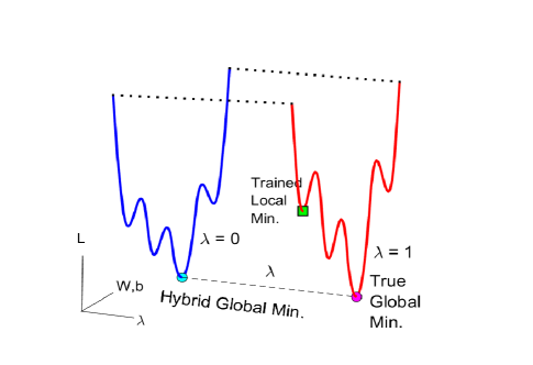
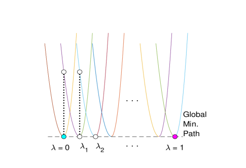
(a)                                                                  (b)

Figure 1: GM Continuation. (a) Trained local minimum is where a conventional training method ends. The surface with the co-train parameter $\lambda$ represents the landscape graph for the hybrid loss function. The method finds the GM below the landscape by continuing the GM at the $\lambda=0$ end all the way to the $\lambda=1$ end. (b) The disc on the line and the disc directly above it are the same parameter point $p$ in the parameter space $\mathbb{R}^{n}$ relative to different continuation parameter values $\lambda$. The former represents the GM for a given $\lambda$, seating at the GM for the loss function. The latter presents the same point lies inside or outside the basin of attraction, or the potential well, of the GM for a forwarding co-train parameter value $\lambda$. If it is inside the GM’s potential well, a gradient descent will lead the point to the new GM. Otherwise, it will leads it to a local minimum of the $\lambda$ value, in which case backtrack correction is applied to continue the process. The goal is to maintain the 100% PR throughout the continuation from start to finish.

In terms of the Poincaré mapping equivalency, for each $\lambda$ we have the equivalent Poincaré map $T_{\lambda}$ for which $\bar{p}_{\lambda}$ is a local minimum for $L_{\lambda}$ if and only if $\bar{p}_{\lambda}$ is a locally stable fixed point of $T_{\lambda}$. Our method is based on the following theorem.

Theorem 1 (Continuation Theorem of Global Minimums).

Assume the perfect global minimum point $p^{\ast}_{\lambda}\in\mathbb{R}^{n}$ of $L_{\lambda}$ exists for every $\lambda\in[0,1]$ and is asymptotically stable for the Poincaré map $T_{\lambda}$. Assume also $T_{\lambda}$ is continuous in $\lambda$ and is differentiable at $p^{\ast}_{\lambda}$. Then the global minimums form a continuous path $\gamma:=\{p^{\ast}_{\lambda}:0\leq\lambda\leq 1\}$ in the training parameter space $\mathbb{R}^{n}$.

Proof.

For each co-train parameter $\lambda\in[0,1]$, let $DT_{\lambda}(p^{\ast}_{\lambda})$ be the linearization of the Poincaré map $T_{\lambda}$ at the fixed point $p^{\ast}_{\lambda}$. Since $p^{\ast}_{\lambda}$ is asymptotically stable for $T_{\lambda}$ which is differentiable, there is an adapted norm ([6]) and a small convex neighborhood $U_{\lambda}$ of the point so that $T_{\lambda}$ is Lipschitz continuous with the Lipschitz constant smaller than 1, i.e. $T_{\lambda}$ is locally contracting. Let $\rho(p)$ be a $C^{\infty}$ cut-off scalar function ([1, 6]) in $U_{\lambda}$. Extend $T_{\lambda}$ from $U_{\lambda}$ to the entire space $\mathbb{R}^{n}$ by

$$T_{\lambda}(p)\to DT_{\lambda}(p^{\ast}_{\lambda})p+\rho(p-p^{\ast}_{\lambda})[T_{\lambda}(p)-DT_{\lambda}(p^{\ast}_{\lambda})p]$$

For small enough neighborhood $U_{\lambda}$, the extended map is a contraction mapping in $\mathbb{R}^{n}$. Without loss of generality, we will use the same notation $T_{\lambda}$ for the extended map. Because the interval $[0,1]$ where $\lambda$ is from is compact, the extended map $T_{\lambda}$ can be made to be uniformly contracting for all $\lambda\in[0,1]$. As a consequence by the Uniform Contraction Mapping Theorem ([1, 6]), for each $\lambda$, $T_{\lambda}$ has a unique fixed point which by construction is exactly the global minimum point $p^{\ast}_{\lambda}$ for $L_{\lambda}$. Also as a consequence to the Uniform Contraction Mapping Theorem, because $T_{\lambda}$ is continuous in $\lambda$, the set of points $\{p^{\ast}_{\lambda}:0\leq\lambda\leq 1\}$ form a continuous path in the training parameter space $\mathbb{R}^{n}$ that is parameterized by the co-train parameter $\lambda$. ∎

Method of Global Minimum Continuation

1. Let $D$ denote the training data for an ANN model. For example, for the MNIST benchmark problem, $D$ is the training data of 60,000 handwritten digits. Train the model by any conventional ways, e.g. stochastic gradient descent (SGD) method, to achieve a considerable positive rate. This divides the data set $D$ into those which are correctly labelled or trained, $D_{t}$, and those which are incorrectly labelled or untrained, $D_{u}$.

2. Create a set of auxiliary data, consisting two parts. One part is exactly the correctly labelled data $D_{t}$. The other part is cloned or duplicated from $D_{t}$ for the same number as $D_{u}$. Specifically, for each incorrectly labelled data from $D_{u}$, pick a trained partner data from $D_{t}$, preferably having the same training label and without repeating. Denote this cloned data set by $\bar{D}_{u}$. As a result, the joint data set $\bar{D}=D_{t}+\bar{D}_{u}$ is perfectly trained for the ANN model, with 100% PR, with the same weight parameter and bias $p=\{W,b\}$ as for the imperfectly trained but true data $D$. The corresponding auxiliary system with $\bar{D}$ is referred to as a training partner. The imperfectly trained parameters $p$ is automatically the global minimum, i.e., $p=\bar{p}^{\ast}$ for the partner system.

3. Introduce a parameter $\lambda$ in the interval $[0,1]$. For each $\lambda$, create an hybrid data from the true data $D$ and the auxiliary partner data $\bar{D}$ by

   $$\mathscr{D}_{\lambda}=(1-\lambda)\bar{D}+\lambda D.$$

   This technique by such weighted average of $\bar{D}$ and $D$ with weight $(1-\lambda)$ and $\lambda$, respectively, is known as homotopy for continuation in dynamical systems ([2, 10]). The trained data $D_{t}$ remains unchanged for all $0\leq\lambda\leq 1$. The part corresponding to the erred data changes from the perfectly trained partner set $\bar{D}_{u}$ at $\lambda=0$ to the original data set $D_{u}$ at $\lambda=1$. If the partnering data are chosen for the same training labels as the partneree data, then the same training labels can be used throughout for all co-train parameters $0\leq\lambda\leq 1$. More generally, one can create a homotopy in the classification space and directly compute the error-rate from the classifying vectors. See Fig.1(a).

4. For the ANN model with the hybrid and co-train data set $\mathscr{D}_{\lambda}$ from $\lambda=0$ to $\lambda=1$, the Continuation Theorem of Global Minimums guarantees that the error-free global minimum at $\lambda=0$ for $\mathscr{D}_{0}=\bar{D}$ is connected all the way through $0<\lambda<1$ to the error-free global minimum at $\lambda=1$ with $\mathscr{D}_{1}=D$, which is what we want for the solution of the training problem. Continuation of the GMs from $\lambda=0$ to $\lambda=1$ can be done by any continuation method. For example, it can be done by solving for equilibrium solutions for the gradient vector field

   $$\nabla L_{\lambda}(p)=0$$

   by Newton’s method or its variations ([8]), starting at the partner system’s global minimum $p^{\ast}_{0}$ at $\lambda=0$. Here below we describe a new method referred to as the gradient-descent tunneling (GDT) method by way of backtrack correction.

Gradient Descent Tunneling: Backtrack Correction

1. Start at $\lambda=0$ where the global minimum $p=p^{\ast}_{0}$ locates for the partner system with training data $\mathscr{D}_{0}=\bar{D}$.

2. Move forward in $\lambda$ to a value $\lambda=a>0$. If $p^{\ast}_{0}$ is inside the gradient-descent’s basin of attraction for the GM $p^{\ast}_{a}$ of the loss function $L_{a}$, then applying a gradient descent algorithm in a few iterations to find the GM $p^{\ast}_{a}$. Fig.1(b) illustrates this case if $a=\lambda_{1}$.

3. If the step size $\lambda=a$ taken if too large, say, $a=\lambda_{2}$ as shown in Fig.1(b), then the parameter $p=p^{\ast}_{0}$ is inside the basin of attraction of a local minimum point. Any gradient descent search will miss the GM $p^{\ast}_{a}$. When this occurs, the PR indicator for the search will be less than 100%. In this case, the step size is reduced to a smaller value, say $a/2$, and then repeat the same step. This procedure is referred to as backtrack correction.

4. The Continuation Theorem of Global Minimums guarantees the convergence of the algorithm. That is, the number of backtrack correction required before the PR becomes 100% is finite. And the convergence also guarantees the GM $p^{\ast}_{1}$ for the true system with data $D$ can be reached in finite steps because the extended Poincaré map $T_{\lambda}$ is a uniform contraction on a compact interval $\lambda\in[0,1]$. In the continuation path to $\lambda=1$ and PR $=$ 100%, there are trained models with sub-100% but high positive rates.

Gradient Descent Tunneling: Adaptive Continuation

1. For computational efficiency, we can speed up the continuation of $\lambda$ by increasing the step-size $a$ if the iteration yields a sequence of consecutive 100% PRs. When combining with the backtrack correction technique, such a continuation should result in an efficient algorithm to find the true global minimum $p^{\ast}_{1}$ at $\lambda=1$.

Cumulative Training

1. As one direct implication of the continuation method, the trained data $D_{t}$ can be viewed as what have been learned by the ANN model and the erred data $D_{u}$ can be viewed as what have to be learnt new data. The co-train continuation method together with GDT can be used to accomplish such memory retention learning tasks so that the model is trained to the new while keeping the old intact.

Figure 2: Complete Segmentation. A projection of the 784-dimension classification space to $\mathbb{R}^{3}$, with $[1,0,0],\ [0,1,0],\ [0,0,1]$ for digits “1”, “2”, “3”. The viewing angle vector is $[1,1,1]$ towards the origin. Top row is for an SGD trained model with 99.88% positive rate and the bottom row is for a fully trained model. The top-right plot presents how the current benchmark model would look like for its final clustering of points. The ANN architecture is 784-100-10.

Result. The continuation method with gradient descent tunneling was implemented on Matlab. Models of two different types of activation functions were used, all having the 784-$n$-10 architecture, and all achieved 100% PR for the MNIST benchmark data, where $n$ is the number of nodes for the only hidden layer. All used the softmax for the output layers’s classification function.

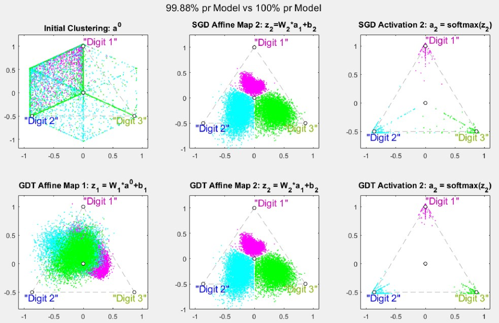
We used the popular ReLU as the activation functions for the hidden layer, with node number $n=$ 100, 80, 60, 40, 20, respectively. The corresponding numbers of parameters in $\{W,b\}$ for the 784-$n$-10 models are 79510, 63610, 47710, 31810, 15910, respectively. Fig.2 shows a comparison between conventionally-trained model and our fully-trained model. The latter achieves a clean and complete partition of the 60,000 training points from the 784-dimensional classification space in a 3D projection for digits 1, 2, and 3. Because ReLU is not differentiable at the origin, the loss function is not differentiable everywhere as required by the continuation theorem. To avoid the non-differentiable points, we chose the initial parameters in $W$ and $b$ randomly with uniform distribution in interval $(-5,5)$. Instead of ${\rm softmax}(x)$, we used a scaled version, ${\rm softmax}(x/100)$ for the output layer’s pooling. But the continuation failed to work for the initials from $(-0.5,0.5)$ together with the standard softmax, most likely because the continuation can’t avoid the non-smooth points of the loss function.

For the second type of activation function, we used a new sigmoid function

$$\sigma(x)=\left\{\begin{array}[]{ll}0,&x\leq 0\\ \tanh^{2}(x/2),&x\geq 0\\ \end{array}\right.$$

This function was derived as the voltage-gated activation function for neuron models which all modelers must agree regardless which approach to take, modeling the conductance or modeling the resistance of the ion channels ([5]). More specifically, the inverse of $\sigma$ over $x>0$ is

$$\rho(x)=\coth^{2}(x/2),\ \ x\geq 0,$$

having the property that both are solutions to the following differential equation

$$\frac{dy}{dx}=\sqrt{y}(1-y),$$

referred to as the switch equation in [5], and the sigmoid function $y=\sigma(x)$ is refereed to as a switch function by extension, for which the state is off if $x\leq 0$ and on if $x>0$. When the ReLU activation function is replaced by the switch function $\sigma$, the continuation method works perfectly for initials of $W,b$ from $(-0.5,0.5)$ together with the standard softmax. Moreover, the convergence with the switch activation function is at least 3 times faster than with the ReLU model for GDT. Also, SGD works faster with the switch function than the ReLU, most likely because of the smoothness difference between them.

Figure 3: Result with Switch Activation. Top two plots show two trainings for the model with the switch activation $\sigma$ with different number of SGD iterations. Thick lines are for the training data and thin lines are for the test data. The bottom plots are similar to the clustering plots of Fig.2 for a fully-trained model.

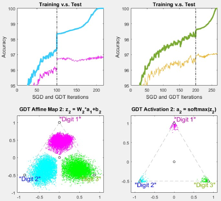
Specifically, Fig.3 shows some results for a 784-100-10 model with the switch function for activation. It shows the accuracy curves for MNIST’s training and test data by the conventionally trained model with SGD and the fully-trained model with GDT. It shows that the final accuracy for test after GDT is always better than the SGD-trained model. It also shows that other than the normal random fluctuations for the test accuracy curve, little can be construed as “overfitting”. The figure also shows the last and the second last segmentations of the transformed training data, with the second last achieved a clearer separation than the model with ReLU from Fig.2.

Discussion. Mathematical data sciences is to solve theoretical and computational scaling problems from small data to large data. The Universal Approximation Theorem by [3, 7] solved the theoretical problem to automate the classification problem by ANN models. For small data, the (stochastic) gradient descent method is able to solve the training problem, i.e. finding the global minimum of a model’s loss function. For large data, finding the global minimum by SGD becomes a game of chance. Our Continuation Theorem should fill this computational gap.

In the parameter $\{W,b\}$ space, there are infinitely many global minimums of a model’s loss function. It can be found by choosing different initial parameters, or by different choices of auxiliary training partners, or by different training batches or iterations with SGD searching. Together with the continuation theorem, it suggests that the global minimums form a hyper-surface continuum in the parameter space. As a result, these global minimums are infinitely many but have zero probability to find by chance via SGD when the data is big and the dimension of the parameter space is big. Our theorem guarantees the convergence of the continuation algorithm if there are enough parameters to ensure the existence of the hybrid global minimums.

Our empirical finding on the size of the ANN models which solved the MNIST training problem suggests that the minimal dimension of the parameter space in which a classification problem is solvable may not be too high, i.e., not suffering the so-called curse of dimensionality. This is because every ANN model has its own intrinsic dimension, like every physics model having finite many state variables for their intrinsic dimensionality. That dimension would fix some upper bound in its number of parameters to fully determine the model. These two numbers plus the number of distinct data whose basins of attraction contain all data points should define some lower bound for the minimal number of parameters in $\{W,b\}$. Of course, this remains as an educated conjecture based on the findings of this paper and the theory of dimension analysis (c.f. [4]).

Our result also suggests the following practices for ANN models. The switch function for activation is better suited than the ReLU is for both SGD training and GDT continuation. Because there are infinitely many global minimums, we can always find those which are good for test data. Thus, we can find one we like and then use GDT to incorporate all test data into one fully-trained model for deployment. Over-fitting is never an issue for good model, good math, and good code.

The error-free training method is applicable for all supervised trainings of ANNs, including convolutional neural networks (CNN), spiking neural networks (SNN). It is even more advantageous because of its relatively small numbers of model parameters required, reducing carbon-footprint for AI training. It can be implemented on platforms from cloud-frame supper computers to microchips on mobile devices. The error-free learning capability of the method will enable AI to fully enter into many fields such as inventory logistic, record keeping, human resource management, fully automated grading for examinations, precision manufacturing, health care management, pharmaceutical and medical expert systems ([15]). It can build error-free modular systems for search engines and for large language models which always involve supervision in various stages. Our result may redirect the question of how accurately an ANN can be trained to how to maximize the potentials of full-trained models.

Declarations

Ethical approval: Not Applied.

Competing interests: None.

Authors’ contributions: Not Applied.

Funding: None.

Availability of data and materials: All trained ANN models mentioned in this article can be downloaded from figshare, https://doi.org/10.6084/m9.figshare.24328756 titled ‘Validation for error-free ANN models on MNIST’. It also contains Matlab mfiles for the SGD training and GDT continuation algorithms.

References

- [1] Chow, S.N. and Hale, J., Methods of Bifurcation Theory, New York, Springer, 1982.
- [2] Chow, S.N., Mallet-Paret, J. and Yorke, J.A., A homotopy method for locating all zeros of a system of polynomials. In Functional Differential Equations and Approximation of Fixed Points: Proceedings, Bonn, July 1978 (pp. 77-88). Berlin, Heidelberg: Springer Berlin Heidelberg, 2006.
- [3] Cybenko, G., Approximation by superpositions of a sigmoidal function. Mathematics of control, signals and systems, 2(4), pp.303-314, 1989.
- [4] Deng, B., An Inverse Problem: Trappers Drove Hares to Eat Lynx, Acta Biotheor, 66, pp.213–242, 2018.
- [5] Deng, B., Neuron model with conductance-resistance symmetry. Physics Letters A, 383(33), p.125976, 2019.
- [6] Deng, B., Theory of invariant manifold and foliation and uniqueness of center manifold dynamics. J. Dyn. Diff. Equat., 2023. https://doi.org/10.1007/s10884-023-10265-3
- [7] Hornik, K., Stinchcombe, M. and White, H., Multilayer feedforward networks are universal approximators. Neural networks, 2(5), pp.359-366, 1989.
- [8] Kelley, C.T., Solving Nonlinear Equations with Newton’s Method, Society for Industrial and Applied Mathematics, 2003.
- [9] LeCun, Y., Bottou, L., Bengio, Y. and Haffner, P., Gradient-based learning applied to document recognition. Proceedings of the IEEE, 86(11), pp.2278-2324, 1998.
- [10] Li, T.Y., Sauer, T. and Yorke, J.A., Numerical solution of a class of deficient polynomial systems. SIAM journal on numerical analysis, 24(2), pp.435-451, 1987.
- [11] Nielsen, M.A., Neural Networks and Deep Learning (Vol. 25). San Francisco, CA, Determination press, 2015.
- [12] Robbins, H. and Monro, S., A Stochastic Approximation Method. The Annals of Mathematical Statistics, 22(3), pp.400–407, 1951.
- [13] Rosenblatt, F., The perceptron: A probabilistic model for information storage and organization in the brain. Psychological review, 65(6), p.386, 1958.
- [14] Image Classification on MNIST. https://paperswithcode.com/sota/image-classification-on-mnist, 2023.
- [15] Yang, J., Shi, R., Wei, D., Liu, Z., Zhao, L., Ke, B., Pfister, H. and Ni, B., MedMNIST v2-A large-scale lightweight benchmark for 2D and 3D biomedical image classification. Scientific Data, 10(1), p.41, 2023.