Reinforcement Unlearning

Abstract.

Machine unlearning refers to the process of mitigating the influence of specific training data on machine learning models based on removal requests from data owners. However, one important area that has been largely overlooked in the research of unlearning is reinforcement learning. Reinforcement learning focuses on training an agent to make optimal decisions within an environment to maximize its cumulative rewards. During the training, the agent tends to memorize the features of the environment, which raises a significant concern about privacy. As per data protection regulations, the owner of the environment holds the right to revoke access to the agent’s training data, thus necessitating the development of a novel and pressing research field, termed reinforcement unlearning. Reinforcement unlearning focuses on revoking entire environments rather than individual data samples. This unique characteristic presents three distinct challenges: 1) how to propose unlearning schemes for environments; 2) how to avoid degrading the agent’s performance in remaining environments; and 3) how to evaluate the effectiveness of unlearning. To tackle these challenges, we propose two reinforcement unlearning methods. The first method is based on decremental reinforcement learning, which aims to erase the agent’s previously acquired knowledge gradually. The second method leverages environment poisoning attacks, which encourage the agent to learn new, albeit incorrect, knowledge to remove the unlearning environment. Particularly, to tackle the third challenge, we introduce the concept of “environment inference” to evaluate the unlearning outcomes.

1. Introduction

Machine learning relies on the acquisition of vast amounts of data, which may encompass sensitive information of individuals. To safeguard the privacy of individual users, data protection regulations have been proposed, e.g., the General Data Protection Regulation (GDPR) (GDPR, 2016), which empowers users to request the removal of their data. It is imperative for model owners to adhere to users’ requests by removing revoked data from their datasets and ensuring that any influence these revoked data may have on the model is eliminated. This process is referred to as machine unlearning (Cao and Yang, 2015; Bourtoule et al., 2021).

While significant progress has been made in conventional machine unlearning (Bourtoule et al., 2021; Guo et al., 2020; Zhang et al., 2022), one area that remains an unfilled gap for unlearning is reinforcement learning (RL). RL is an essential research field in machine learning due to its ability to address complex decision-making problems in dynamic environments (Wang et al., 2022a). In RL, the primary objective is to train an intelligent entity, known as an agent, to interact with the environment through a specific policy. This policy guides its actions based on the current state. With each action taken, the agent receives a reward and consequently updates its state, creating an experience sample used to update its policy. The ultimate aim of the agent is to learn an optimal policy that maximizes its cumulative rewards over time.

However, in the course of RL, agents tend to memorize features of their environments, raising substantial security concerns. Consider an RL agent designed for providing navigation guidance through real-time data from Google Maps. During its training, the agent learns from a dynamic environment using Google Street Views for its photographic content (Mirowski et al., 2018). However, privacy issues may arise when the agent inadvertently learns and stores sensitive information, such as the locations of restricted areas. Without a forgetting mechanism, this poses a significant privacy risk, potentially compromising the anonymity of individuals and organizations.

In addition, the agent’s ability to forget is also crucial for ensuring the security of autonomous vehicles. A security challenge arises from malicious entities that exploit the mapping system by registering fraudulent businesses on Google Maps (Huang et al., 2017). Their aim is to redirect organic search traffic away from legitimate establishments and steer it towards profit-driven scams. When training an autonomous driving agent, utilizing maps tainted by such fraudulent entries can lead to suboptimal user experiences or even result in fatal consequences. Thus, the need for the RL agent to forget such sensitive or incorrect information gives rise to a novel research field, which we term as reinforcement unlearning.

Conventional machine unlearning methods are not directly applicable to reinforcement unlearning due to fundamental differences in their learning paradigms. In machine learning, unlearning involves removing specific data samples from the static training set, where data samples are independently and identically distributed. In contrast, RL is a dynamic and sequential decision-making process, where agents interact with an environment in a series of actions, and agents’ experience samples are temporally dependent.

Additionally, reinforcement unlearning is distinct from privacy-preserving RL (Vietri et al., 2020; Garcelon et al., 2021). Reinforcement unlearning aims to selectively erase learned knowledge from the agent’s memory, ensuring the privacy of environment owners, while privacy-preserving RL focuses on preserving the agent’s personal information. In essence, reinforcement unlearning presents three specific challenges.

• How can we unlearn an environment from the agent’s policy? In machine unlearning, a data owner can specify which data samples should be removed. However, in reinforcement unlearning, the environment owner cannot access the experience samples. The difficulty arises as these samples are dynamically accumulated during the agent’s interactions with the environment, and samples are managed by the agent. Thus, the key challenge lies in effectively associating the environment that needs to be unlearned with the corresponding experience samples.

• How can we prevent a degradation in the agent’s performance after unlearning? In conventional machine unlearning, removing a sample may lead to a decrease of performance. It is more challenging in reinforcement unlearning as unlearning an environment requires forgetting a significant number of experience samples. Ensuring that the agent maintains its performance on the retained environments becomes a considerable challenge.

• How can we evaluate the effectiveness of reinforcement unlearning? In machine unlearning, one commonly used evaluation is using membership inference attack (Shokri et al., 2017; Ye et al., 2022; Salem et al., 2023) to assess if the model has discarded the revoked data. However, this methodology cannot be directly applied to reinforcement unlearning, as the environment owner cannot specify which samples should be unlearned. This poses a challenge in evaluating the effectiveness of reinforcement unlearning and in determining if the agent has been over- or under-unlearned.

To address these challenges, we propose two distinct unlearning methods: decremental reinforcement learning and environment poisoning. Decremental reinforcement learning involves deliberately erasing an agent’s learned knowledge about a specific environment. This method finds practical applications in scenarios where certain environments become obsolete or need to be forgotten due to privacy concerns. Environment poisoning-based method aims to create poisoning experience samples by modifying the unlearning environment. This method ensures that the agent’s performance in other environments remains unaffected, eliminating any negative impact on its overall capabilities. This method finds application in situations where attacks or misinformation may be present. Both methods enable an agent to unlearn specific environments while maintaining its performance in others, thereby tackling the first two challenges. To tackle the third challenge, we utilize environment inference to infer an agent’s training environment by observing its behavior. If the inference result after unlearning shows a substantial degradation compared to the result before unlearning, it is indicative that the agent has effectively unlearned that environment.

In summary, we make three main contributions:

• We provide a valuable step forward in machine unlearning by pioneering the research of reinforcement unlearning. The concept of reinforcement unlearning that selectively forgets learned knowledge of the training environment from the agent’s memory offers novel insights and lays a foundation for future research in this emerging domain.

• Reinforcement unlearning exposes an impactful vulnerability of RL – the risk of exposing the privacy of the environment owner. This vulnerability can disclose sensitive information about the environment owner’s preferences and intentions. We introduce two innovative reinforcement unlearning methods: decremental RL-based and environment poisoning-based approaches.

• With limited prior research in reinforcement unlearning, to confirm the unlearning results, we introduce a novel evaluation approach, “environment inference”. By visualizing the unlearning results, this approach provides an intuitive and effective means of measuring the efficacy of unlearning techniques.

2. Preliminaries

Reinforcement Learning.  The primary objective of RL is to learn an optimal policy for the agent, enabling it to maximize the total accumulated reward and accomplish the task optimally. In the context of deep reinforcement learning (DRL), the policy is typically represented by a deep neural network.

Formally, a learning environment is commonly formulated by the tuple $\mathcal{M}=\langle\mathcal{S},\mathcal{A},\mathcal{T},r\rangle$ (Mnih and et al., 2015). Here, $\mathcal{S}$ and $\mathcal{A}$ denote the state and action sets, respectively, while $\mathcal{T}$ represents the transition function, and $r$ represents the reward function. At each time step $t$, the agent, given the current environmental state $s_{t}\in\mathcal{S}$, selects an action $a_{t}\in\mathcal{A}$ based on its policy $\pi(s_{t},a_{t})$. This action causes a transition in the environment from state $s_{t}$ to $s_{t+1}$ according to the transition function: $\mathcal{T}(s_{t+1}|s_{t},a_{t})$. The agent then receives a reward $r_{t}(s_{t},a_{t})$, along with the next state $s_{t+1}$. This tuple of information, denoted as $(s_{t},a_{t},r_{t}(s_{t},a_{t}),s_{t+1})$, is collected by the agent as an experience sample utilized to update its policy $\pi$. Typically, the policy $\pi$ is implemented using a Q-function: $Q(s,a)$, estimating the accumulated reward the agent will attain in state $s$ by taking action $a$. Formally, the Q-function is defined as:

(1) $$Q_{\pi}(s,a)=\mathbb{E}_{\pi}[\sum^{\infty}_{i=1}\gamma^{i}\cdot r(s_{i},a_{i})|s_{i}=s,a_{i}=a],$$

where $\gamma$ represents the discount factor.

In deep reinforcement learning, a neural network is employed to approximate the Q-function, denoted as $Q(s,a;\theta)$, where $\theta$ represents the weights of the neural network. The neural network takes the state $s$ as input and produces a vector of Q-values as output, with each Q-value corresponding to an action $a$. To learn the optimal values of $Q(s,a;\theta)$, the weights $\theta$ are updated using a mean squared error loss function $\mathcal{L}(\theta)$.

(2) $$\mathcal{L}=\frac{1}{|B|}\sum_{e\in B}[(r(s_{t},a_{t})+\gamma\max_{a_{t+1}}Q(s_{t+1},a_{t+1};\theta)-Q(s_{t},a_{t};\theta))^{2}],$$

where $e=(s_{t},a_{t},r(s_{t},a_{t}),s_{t+1})$ is an experience sample showing a state transition, and $B$ consists of multiple experience samples used to train the neural network.

Machine Unlearning.  Machine unlearning focuses on removing specific data samples or learned knowledge from a trained model. Unlike model training, unlearning aims to erase the impact of certain data samples on the model’s behavior. A straightforward unlearning method involves removing the revoked data and retraining the model from scratch. However, this approach is computationally challenging. To improve computational efficiency, several machine unlearning methods have been proposed. SISA (Sharded, Isolated, Sliced, and Aggregated) is one of the most prevalent methods (Bourtoule et al., 2021), aiming to divide the training set into disjoint shards and train each shard model separately. When a revoke request is received, only the corresponding shard model is retrained.

When combining machine unlearning with reinforcement learning, a novel concept called reinforcement unlearning is introduced. This concept revolves around the selective removal or modification of the agent’s acquired knowledge within the context of reinforcement learning, offering unique insights and challenges in the dynamic environment of sequential decision-making tasks.

3. Reinforcement Unlearning

3.1. Problem Statement and Threat Model

Problem Definition.  The definition of “forgetting” is application-dependent, leading to different desiderata and priorities in various scenarios (Kurmanji et al., 2023). For example, in a privacy-centric application, the main goal of unlearning user data is to ensure that the unlearned model has no exposure to the data, and a successful membership inference attack would reveal that the data is not in the training set for the unlearned model. Conversely, in a bias-removing application, the aim of unlearning is to prevent the unlearned model from predicting the assigned labels of the forgotten data, as these labels may indicate unintended and biased behavior.

The objective of reinforcement unlearning is to eliminate the influence of a specific environment on the agent, i.e., “forgetting an environment”. We define “forgetting an environment” as equivalent to “performing deterioratively in that environment”. This definition aligns with common sense. For example, when we have thoroughly explored a place and are highly familiar with it, we can efficiently find things within it, resulting in high performance. Conversely, when we have forgotten a place, our ability to locate things diminishes, leading to deteriorative performance.

It is worth noting that we cannot simply adopt the concept of “forgetting” from conventional machine unlearning, which often involves retraining the model from scratch without the revoked data. This is because reinforcement unlearning operates within a distinct learning paradigm, such as sequential decision making and dynamic learning. For instance, even if we were to retrain an agent from scratch without including a specific unlearning environment, there’s a possibility that the agent still performs well in that environment. However, this positive performance could be exploited by adversaries to deduce critical information about that environment. This clearly contradicts the fundamental objective of safeguarding the environment owner’s privacy in reinforcement unlearning.

Formally, let us consider a set of $n$ learning environments:
$\{\mathcal{M}_{1},\ldots,\mathcal{M}_{n}\}$. Each environment $\mathcal{M}_{i}$ has the same state and action spaces but differs in state transition and reward functions. Consider the target environment to be unlearned as $\mathcal{M}_{u}=\langle\mathcal{S}_{u},\mathcal{A}_{u},\mathcal{T}_{u},r\rangle$, denoted as the ‘unlearning environment’. The set of remaining environments, denoted as $\{\mathcal{M}_{1},\ldots,\mathcal{M}_{u-1},\mathcal{M}_{u+1},\ldots,\mathcal{M}_{n}\}$, will be referred to as the ‘retaining environments’. Given a learned policy $\pi$, the goal is to update the policy $\pi$ to $\pi^{\prime}$ such that the accumulated reward obtained in $\mathcal{M}_{u}$ is minimized:

(3) $$\min_{\pi^{\prime}}||Q_{\pi^{\prime}}(s)||_{\infty},$$

where $s\in\mathcal{S}_{u}$, while the accumulated reward received in the retaining environments remains the same:

(4) $$\min_{\pi^{\prime}}||Q_{\pi^{\prime}}(s)-Q_{\pi}(s)||_{\infty},$$

where $s\notin\mathcal{S}_{u}$. We assume that the owner of the trained RL model can access $\mathcal{M}_{u}$ and gather trajectories within $\mathcal{M}_{u}$. A trajectory $\tau$ is denoted as a sequence of state-action pairs: $\tau=((s_{1},a_{1}),\ldots,(s_{k},a_{k}))$, where $k$ represents the length of the trajectory.

The assumption of the model owner having access to the unlearning environment $\mathcal{M}_{u}$ is reasonable, as $\mathcal{M}_{u}$ is an integral part of the training data used by the model owner to train the agent. When an unlearning request is initiated, the model owner employs the proposed unlearning methods, leveraging the unlearning environment $\mathcal{M}_{u}$, to execute the unlearning process. Subsequently, the model owner physically removes $\mathcal{M}_{u}$. This approach ensures that the unlearning is performed using the relevant environment data under the ownership of the user, maintaining a practical and privacy-conscious procedure.

Threat Model.  Reinforcement unlearning primarily focuses on mitigating the influence of a designated unlearning environment on the trained agent. This essentially involves safeguarding the distinctive features of that environment by thwarting a particular type of attack, namely environment inference attacks. In these attacks, adversaries seek to infer a learning environment by closely observing the actions of the agent within that specific environment. Formally, consider the unlearning environment as $\mathcal{M}_{u}=\langle\mathcal{S}_{u},\mathcal{A}_{u},\mathcal{T}_{u},r\rangle$ and the unlearned policy as $\pi^{\prime}$. The adversary’s objective is to infer the transition function $\mathcal{T}_{u}$ by accessing $\mathcal{S}_{u}$, $\mathcal{A}_{u}$, $r$, and $\pi^{\prime}$.

It is essential to note that the environment inference attack differs significantly from conventional membership inference attacks in machine learning. Traditional membership inference attacks typically involve point-level inference, where the focus is on deducing information about an individual sample. In contrast, the environment inference attack operates at the object level, concentrating on the inference of features characterizing an entire environment that encompasses a substantial number of samples. This distinction underscores the unique nature of the environment inference attack, as it extends its scope beyond individual data points to involve the broader context of environments, introducing a new dimension to the evaluation methodology for reinforcement unlearning.

Methods Overview.  Both decremental reinforcement learning-based method and the poisoning-based method share the common aim of intentionally degrading the agent’s performance within the unlearning environment while preserving its performance in other environments. However, they employ distinct strategies to achieve this outcome. The decremental reinforcement learning-based method involves updating the agent by minimizing its reward specifically in the unlearning environment. This is achieved through iterative adjustments to the agent’s policy, aiming to reduce its effectiveness within the unlearning environment. In contrast, the environment poisoning-based method focuses on modifying the unlearning environment itself. This method involves introducing deliberate changes to the state transition function of the environment and subsequently updating the agent in this modified environment. The intention is to disrupt the agent’s learned behavior in the unlearning environment.

3.2. Decremental RL-based Method

The implementation of this method involves two main steps. The first one is the exploration of the unlearning environment $\mathcal{M}_{u}$. Initially, the agent is allowed to explore the unlearning environment, collecting experience samples specific to that environment. The nature of this exploration depends on the scenario. For instance, in the grid-world setting, the agent might traverse the unlearning grid using a random walk for a predefined number of steps. In the aircraft-landing scenario, it could involve the airplane making random landings within the unlearning environment. The second step is fine-tuning the agent. Following the exploration phase, the agent is fine-tuned using the collected experience samples. This fine-tuning process employs a newly defined loss function (Eq. 5) to update the policy $\pi^{*}$ with the experience samples accumulated in the first step. This loss function is carefully designed to ensure that the agent’s performance within the unlearning environment $\mathcal{M}_{u}$ degrades while preserving its performance in other environments. Essentially, it guides the agent to unlearn the knowledge associated with the unlearning environment.

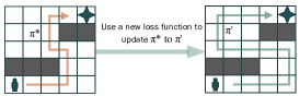
Figure 1. The schematic diagram of the decremental reinforcement learning-based method

To accomplish the aim of unlearning, we establish an optimization objective to guide the unlearning process (Eqs. 3 and 4). We also introduce a new loss function (Eq. 5) that will be used to update the agent. This loss function is designed to minimize the influence of the previously learned knowledge and encourage the agent to modify its existing policy. By incorporating this loss function into the training procedure, we can steer the agent’s learning process towards unlearning the knowledge from the given environment.

(5) $$\mathcal{L}_{u}=\mathbb{E}_{s\sim\mathcal{S}_{u}}[||Q_{\pi^{\prime}}(s)||_{\infty}]+\mathbb{E}_{s\not\sim\mathcal{S}_{u}}[||Q_{\pi^{\prime}}(s)-Q_{\pi}(s)||_{\infty}].$$

In Eq. 5, the first term encourages the new policy $\pi^{\prime}$ to work deficiently in the unlearning environment $\mathcal{M}_{u}$, while the second term drives the new policy $\pi^{\prime}$ to have the same performance as the current policy $\pi$ in other environments. Notably, the two terms in Eq. 5 have favorable properties. The first term directs an agent to search and attempt different policies to sufficiently explore the state space of environment $\mathcal{M}_{u}$. Thus, $\mathcal{M}_{u}$ can be adequately unlearned. This property is particularly useful when $\mathcal{M}_{u}$ is a sparse reward setting, i.e., the reward is $0$ in most of the states in $\mathcal{S}_{u}$. The second term motivates an agent to modify policies, instead of randomly changing its behavior. This property ensures that the agent performs consistently in those states which are not in $\mathcal{S}_{u}$. It is essential to highlight that the accurate computation of the second term is infeasible due to its involvement with all states except $\mathcal{S}_{u}$. Thus, during implementation, we uniformly select a consistent set of states across all environments, excluding $\mathcal{M}_{u}$. This approach is taken to mitigate computational burden and ensure a balanced impact on performance preservation across the remaining environments.

The decremental RL-based method is formally described as follows. First, the agent explores the unlearning environment using a random policy. This policy ensures that the agent takes each action with equal probability. Adopting a random policy ensures a comprehensive exploration of the unlearning environment. If the agent were to use a well-established policy from its training, there is a risk of swift achievement of the target, potentially resulting in insufficient collection of experience samples within the unlearning environment. This strategic use of a random policy enables the effective collection of diverse experiences crucial for the unlearning process. For instance, in the grid world setting, where the agent has four possible actions (moving up, down, left, and right), the random policy dictates that, in each grid (i.e., state), the agent has an equal likelihood of selecting any of the four directions. As the agent progresses in its exploration, in each time step $t$, after taking an action $a_{t}$, it receives a corresponding reward $r_{t}$. Coupled with the current state $s_{t}$ and the subsequent state $s_{t+1}$, the agent effectively creates an experience sample in the form of $(s_{t},a_{t},r_{t},s_{t+1})$. In our method, the agent is directed to explore the unlearning environment for a specified number of steps, denoted as $m$. Consequently, the agent accumulates a total of $m$ experience samples: $(s_{1},a_{1},r_{1},s_{2}),\ldots,(s_{m},a_{m},r_{m},s_{m+1})$. In the second step, the agent employs these collected experience samples to fine-tune its current optimal policy $\pi^{*}$ to a new policy $\pi^{\prime}$ by minimizing the custom loss function defined in Eq. 5.

Convergence Analysis of the Method.  We proceed with examining the convergence of the method by conducting a separate analysis for each term in Eq. 5.

For the first term in Eq. 5, let $y_{\pi}=r(s,\pi(s))+\gamma max_{\pi(s^{\prime})}Q(s^{\prime},\pi(s^{\prime}))$ and $\delta_{\pi}=y_{\pi}-Q(s,\pi(s))$, where $s^{\prime}$ denotes the next state. Then, the loss function in Eq. 2 can be rewritten as:

(6) $$\mathcal{L}=\mathbb{E}_{s\sim\mathcal{S}}[\delta_{\pi}].$$

Similarly, the first term in Eq. 5 can also be rewritten as: $\mathbb{E}_{s\sim\mathcal{S}_{u}}[|y_{\pi^{\prime}}-\delta_{\pi^{\prime}}|]$. Based on the triangle inequality, we have:

(7) $$\mathbb{E}_{s\sim\mathcal{S}_{u}}[|y_{\pi^{\prime}}-\delta_{\pi^{\prime}}|]\leq\mathbb{E}_{s\sim\mathcal{S}_{u}}[|y_{\pi^{\prime}}|]+\mathbb{E}_{s\sim\mathcal{S}_{u}}[|\delta_{\pi^{\prime}}|].$$

As the convergence of the learning on the loss function in Eq. 6 has been both theoretically and empirically proven (Mnih et al., 2013; Tosatto et al., 2017; Fan et al., 2020), we can also conclude the convergence of $\mathbb{E}_{s\sim\mathcal{S}_{u}}[|\delta_{\pi^{\prime}}|]$ in Eq. 7. For the first term in the right of Eq. 7, $\mathbb{E}_{s\sim\mathcal{S}_{u}}[|y_{\pi^{\prime}}|]$, as it is computed by accumulating the previously collected discounted rewards (Eq. 1 and 2), the term converges if the rewards are bounded. The reward bound can be acquired by proper definition, i.e., $r\in[-R_{max},R_{max}]$. Thus, as both $\mathbb{E}_{s\sim\mathcal{S}_{u}}[|y_{\pi^{\prime}}|]$ and $\mathbb{E}_{s\sim\mathcal{S}_{u}}[|\delta_{\pi^{\prime}}|]$ converge, $\mathbb{E}_{s\sim\mathcal{S}_{u}}[|y_{\pi^{\prime}}-\delta_{\pi^{\prime}}|]$ also converges, i.e., $\mathbb{E}_{s\sim\mathcal{S}_{u}}[||Q_{\pi^{\prime}}(s)||_{\infty}]$ converges.

For the second term in Eq. 5, to analyze its convergence, we need the following theorem.

Theorem 1 (Error Propagation (Tosatto et al., 2017)).

Let $(\pi_{i})^{K}_{i=0}$ be a sequence of policies with regard to the sequence $(Q_{i})^{K}_{i=0}$ of Q-functions learned using a fitted Q-iteration. Then, the following inequality holds.

$$||Q_{i}-Q^{*}||_{\infty}\leq||\xi_{i-1}||_{\infty}+\gamma||Q_{i-1}-Q^{*}||_{\infty}+\zeta||Q_{i-1}||_{\infty},$$

where $Q^{*}$ is the optimal value function, $\xi_{i}$ denotes the approximation error: $\xi_{i}=T^{\pi_{i}}Q_{i}-Q_{i+1}$ which is also bounded, $T$ is the Bellman operator, and $\zeta$ is a constant.

Theorem 1 provides evidence that the disparity between the learned Q-function and the optimal Q-function diminishes as the learning process advances. This reduction signifies convergence, given that the Q-function, denoted as $Q$, remains uniformly bounded by $\frac{R_{max}}{1-\gamma}$ for any policy $\pi$ (Tosatto et al., 2017). Consequently, if the number of learning iterations is sufficiently large, the method converges.

In our problem, the second term in Eq. 5, $\mathbb{E}_{s\not\sim\mathcal{S}_{u}}[||Q_{\pi^{\prime}(s)}(s)-Q_{\pi(s)}(s)||_{\infty}]$, is intended to minimize the performance discrepancy between the unlearned policy $\pi^{\prime}$ and the well-trained policy $\pi$ across all environments except $\mathcal{M}_{u}$. In this context, the well-trained policy $\pi$ can be considered as the optimal policy, while the unlearned policy $\pi^{\prime}$ represents the policy we aim to learn. Notably, this learning process is analogous to the one described in Theorem 1, implying that the second term also exhibits convergence.

3.3. Environment Poisoning-based Method

This method is implemented by modifying the unlearning environment itself. This modification can include various changes, i.e., the poisoning actions, such as altering the layout in the grid world scenario by adding or removing obstacles and repositioning targets within the environment. After these changes are introduced, the agent is updated in this modified environment. This method aims to influence the agent’s policy learning by creating a situation where its previously learned knowledge becomes less effective, particularly within the context of the unlearning environment.

Specifically, this method consists of three distinct steps. Firstly, we apply a random poisoning strategy to alter the transition function of the unlearning environment. Secondly, the agent learns a new policy in this modified environment. Lastly, based on the agent’s learned policy, we update the poisoning strategy and re-poison the unlearning environment. These three steps are iteratively repeated until a predetermined number of poisoning epochs is reached, effectively refining the unlearning process. By employing this iterative approach, the method enhances the agent’s ability to unlearn specific experiences associated with the targeted unlearning environment. The schematic diagram of this method is presented in Figure 2, illustrating that the targeted unlearning environment $\mathcal{M}_{u}$ is altered to a new one $\mathcal{M}^{\prime}_{u}$ with strategically introduced perturbations, e.g., adding fake obstacles, and the agent is retrained in this poisoned environment to learn a new policy $\pi^{\prime}$.

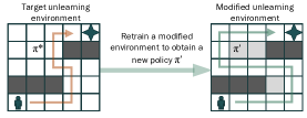
Figure 2. The schematic diagram of the environment poisoning-based method

Let us consider the learned policy as $\pi^{*}$, which is regarded as the optimal policy. To refine the agent’s policy, we manipulate the given environment $\mathcal{M}_{u}$. The manipulation of $\mathcal{M}_{u}$ involves poisoning the transition function $\mathcal{T}_{u}(s^{\prime}|s,a)$ (Xu et al., 2022), where $\mathcal{M}_{u}=\langle\mathcal{S}_{u},\mathcal{A}_{u},\mathcal{T}_{u},r\rangle$. We introduce a poisoned transition function denoted as $\hat{\mathcal{T}}_{u}(\hat{s}^{\prime}|s,a)$. After the agent takes action $a$ in state $s$, instead of observing the intended state $s^{\prime}$, it will observe the manipulated state $\hat{s}^{\prime}$. The challenge now lies in determining the appropriate state $\hat{s}^{\prime}$, which can mislead the agent’s learning process. To address this, we define a new learning environment for poisoning, denoted as $\mathcal{M}_{p}=\langle\mathcal{O},\mathcal{G},\mathcal{P},\mathcal{R}\rangle$. By constructing this new environment, we can manipulate the state transitions experienced by the agent, thus guiding its learning process in a desired manner.

• $\mathcal{O}$ denotes the set of poisoning states. Each state $\pi_{i}\in\mathcal{O}$ is the policy used by the agent during the $i$-th poisoning epoch.

• $\mathcal{G}$ is the set of poisoning actions. A poisoning action $g\in\mathcal{G}$ signifies a modification made to the transition function of the unlearning environment $\mathcal{T}_{u}$. This modification determines which state should be presented to the agent as the new state.

• $\mathcal{P}:\mathcal{O}\times\mathcal{G}\times\mathcal{O}\rightarrow[0,1]$ defines the poisoning state transition. It describes how the agent adjusts its policy in response to poisoning actions. Specifically, $\mathcal{P}(\pi^{\prime}|\pi,g)$ is the probability of the agent transitioning from policy $\pi$ to policy $\pi^{\prime}$ when the unlearning environment’s transition function is modified by $g$.

• $\mathcal{R}:\mathcal{O}\times\mathcal{G}\times\mathcal{O}\rightarrow\mathbb{R}$ represents the reward function, which serves two purposes. Firstly, it quantifies the disparity between the current policy $\pi_{i}$ and the updated policy $\pi^{\prime}$ in the unlearning environment $\mathcal{M}_{u}$. Secondly, it incorporates the rewards obtained by the agent in other environments while utilizing $\pi_{i}$. Specifically, the reward function is defined as

  (8) $$\mathcal{R}_{i}:=\lambda_{1}\Delta(\pi_{i}(s_{i})||\pi^{\prime}(s_{i}))+\lambda_{2}\sum_{s\not\sim\mathcal{S}_{u}}\sum_{a}\pi_{i}(s,a)r(s,a).$$

  $\mathcal{R}_{i}$ represents the reward received during the $i$-th poisoning epoch. The term $\Delta(\pi_{i}(s_{i})||\pi^{\prime}(s_{i}))$ indicates the difference between $\pi_{i}(s_{i})$ and $\pi^{\prime}(s_{i})$. Here, $\pi_{i}(s_{i})$ represents the probability distribution over the available actions in state $s_{i}$ under policy $\pi_{i}$. This difference can be measured using either KL-divergence or cosine similarity. Coefficients $\lambda_{1}$ and $\lambda_{2}$ are introduced to balance the two terms. Note that precisely computing the second term is computationally infeasible due to the involvement of states from all environments except $\mathcal{M}_{u}$. Thus, similar to the decremental RL-based method, in the implementation of the poisoning-based method, a uniform selection of states across all the environments, except $\mathcal{M}_{u}$, is performed in each poisoning epoch.

Algorithm 1 The poisoning-based method

0:  The learned policy $\pi^{*}$, the learning tasks $\mathcal{M}_{1},...,\mathcal{M}_{n}$, and the unlearning task $\mathcal{M}_{u}$;

0:  A refined policy $\hat{\pi}$;

1:  for poisoning epoch $i=1,...,m$ do

2:     Select a poisoning action $g_{i}$ from $\mathcal{G}$;

3:     Alter the transition function of the unlearning task from $\hat{\mathcal{T}}_{u,{i-1}}$ to $\hat{\mathcal{T}}_{u,i}$ based on $g_{i}$;

4:     The agent learns a policy $\pi_{i}$ according to $\hat{\mathcal{T}}_{u,i}$;

5:     Receive reward $\mathcal{R}_{i}$;

6:     Update poisoning strategy using samples $(\pi_{i-1},g_{i},\pi_{i},\mathcal{R}_{i})\in\mathcal{B}$ by optimizing loss function Eq. 2;

7:  end for

8:  return  $\hat{\pi}\leftarrow\pi_{m}$;

The proposed poisoning-based method is outlined in Algorithm 1. In each poisoning epoch $i$, we take the first step by choosing a poisoning action $g_{i}$ to modify the transition function of the unlearning environment (Lines 1-3). The selection process can be implemented using an $\epsilon$-greedy strategy, where the best action is chosen with a probability of $1-\epsilon$, and the remaining actions are chosen uniformly with a probability of $\frac{\epsilon}{|\mathcal{G}|-1}$. Here, the “best action” denotes the action that results in the highest Q-value, signifying the maximum expected future reward. This criterion guides the agent to identify the most effective way to modify the unlearning environment, ensuring optimal adjustments based on the expected outcomes.

Next, the agent performs the second step by learning a new policy $\pi_{i}$ in the altered environment (Line 4). This learning phase can be performed using any deep reinforcement learning algorithm, such as deep Q-learning (Mnih et al., 2013). Once $\pi_{i}$ is learned, we execute the third step by evaluating the reward using Eq. 8 and updating the poisoning strategy using samples $(\pi_{i-1},g_{i},\pi_{i},\mathcal{R}_{i})$ from batch $\mathcal{B}$ (Lines 5 and 6). The update process is carried out using the DDPG algorithm (Lillicrap et al., 2016). After all poisoning epochs are completed, we obtain a refined policy $\hat{\pi}$ (Line 8), which allows the agent to perform poorly in the unlearning environment $\mathcal{M}_{u}$, while maintaining satisfactory performance in other environments.

Convergence Analysis of the Method.  Algorithm 1 represents a deep RL algorithm employed by the model owner. This algorithm utilizes the agent’s policies as states, the modification of the unlearning environment as actions, and the performance of the agent’s policies in the environments as rewards. The interaction between the algorithm and the agent’s learning process is illustrated in Figure 3. In this figure, the model owner is engaged in learning how to poison the unlearning environment $\mathcal{M}_{u}$, while the agent is concurrently learning within the poisoned environment $\mathcal{M}^{\prime}_{u}$.

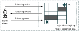
Figure 3. The interaction between agent learning and model owner poisoning. The owner observes the poisoning states about the unlearning environment $\mathcal{M}_{u}$, takes poisoning actions against $\mathcal{M}_{u}$, and receives poisoning rewards. The agent, on the other hand, is learning in the poisoned environment.

Given that our primary concern lies in the performance of the agent’s policies, our analysis primarily revolves around these policies. Each policy $\pi$ is associated with a state distribution denoted as $\mu_{\pi}$, which can be defined as:

$$\mu_{\pi}:=(1-\gamma)\sum^{\infty}_{t=0}\gamma^{t}\mathbb{P}[s_{t}=s|s_{0}\sim d_{0},\pi],$$

where $d_{0}$ is the initial state distribution and $\mu_{\pi}>0$ for each state $s$. Here, $\mu_{\pi}$ satisfies the following Bellman flow constraints (Rakhsha et al., 2021):

(9) $$\mu_{\pi}=(1-\gamma)d_{0}+\gamma\sum_{s^{\prime}}\mathcal{T}(s^{\prime}|\pi(s^{\prime}),s)\mu_{\pi(s^{\prime})}.$$

Then, the score of policy $\pi$ can be defined as:

$$\rho_{\pi}(\mathcal{M},d_{0}):=\sum_{s}\mu_{\pi}(s)r(s,\pi(s)).$$

The policy score $\rho_{\pi}$ quantifies the quality of a policy $\pi$, with a higher score indicating a better policy. Specifically, $\rho_{\pi}$ has the following property.

Lemma 1 (Even-dar et al. (Even-dar et al., 2004)).

For two policies $\pi$ and $\pi^{\prime}$, the following equation holds: $\rho_{\pi}-\rho_{\pi^{\prime}}=\sum_{s\in\mathcal{S}}\mu_{\pi^{\prime}}(s)(Q_{\pi}(s,\pi(s))-Q_{\pi}(s,\pi^{\prime}(s)))$.

Let us examine the expression $Q_{\pi}(s,\pi(s))-Q_{\pi}(s,\pi^{\prime}(s))$. To simplify the analysis, we introduce a seminorm called the span. The span of $Q$ is defined as $sp(Q)=\max_{i}Q(s_{i},a_{i})-\min_{j}Q(s_{j},a_{j})$. This seminorm measures the maximum difference between the highest and lowest values of the function $Q$ across different states and actions. Certainly, we have: $Q_{\pi}(s,\pi(s))-Q_{\pi}(s,\pi^{\prime}(s))\leq sp(Q_{\pi})$. Then, we have: $\rho_{\pi}-\rho_{\pi^{\prime}}\leq sp(Q_{\pi})|\mathcal{S}|\sum_{s\in\mathcal{S}}\mu_{\pi^{\prime}}(s)$.

Based on Eq. 1 and 9, it can be inferred that the span $sp(Q_{\pi})$ is limited by the cumulative reward, while $\mu_{\pi^{\prime}}$ is bounded by the transition function. The reward is predefined by users, and the initial state distribution $d_{0}$ remains fixed for a given environment. Thus, the only variable that influences the difference in policy scores, $\rho_{\pi}-\rho_{\pi^{\prime}}$, is the transition function dictated by the environment. This rationale underscores why we opt for environment-poisoning as our unlearning method.

3.4. Comparison of the Two Methods

We compare the two methods in their ability of overcoming the “over-unlearning” and “catastrophic forgetting” issues.

In the context of a set of environments $\{\mathcal{M}_{1},...,\mathcal{M}_{n}\}$ and an unlearning environment $\mathcal{M}_{u}$, the objective of the decremental RL-based method is to minimize the agent’s return specifically in $\mathcal{M}_{u}$ while ensuring that the return in the remaining environments remains unaffected. In contrast, the poisoning-based method aims to develop a strategy to modify the unlearning environment $\mathcal{M}_{u}$ into $\mathcal{M}^{\prime}_{u}$ and subsequently fine-tune the agent within this modified environment. The objective is to ensure that the agent adapts well to $\mathcal{M}^{\prime}_{u}$ while exhibiting poor performance in the original unlearning environment $\mathcal{M}_{u}$. Thus, the key distinction between the two methods lies in their approaches. The decremental RL-based method focuses on erasing the knowledge acquired by the agent in $\mathcal{M}_{u}$, while the poisoning-based method encourages the agent to learn in a new but altered environment, i.e., $\mathcal{M}^{\prime}_{u}$.

One advantage of the poisoning-based method over the decremental reinforcement learning-based method is its ability to address the over-unlearning issue associated with the latter. The decremental reinforcement learning-based method may inadvertently suffer from over-unlearning, which occurs when the deep reinforcement learning model is fine-tuned to degrade the agent’s learning performance in $\mathcal{M}_{u}$. This issue is also observed in conventional machine unlearning scenarios (Bourtoule et al., 2021). Even if efforts are made to restrict the deterioration to $\mathcal{M}_{u}$, it may still affect other environments due to the shared distribution among them. However, the poisoning-based method inherently avoids this issue by focusing on enabling the agent to learn new knowledge rather than intentionally forgetting existing knowledge. Thus, the poisoning-based method has the potential to achieve superior performance in non-unlearning environments compared to the decremental RL-based method.

A valid concern regarding the poisoning-based method is the potential occurrence of catastrophic forgetting, which arises when the continual updating of the deep reinforcement learning model results in the overwriting of previously acquired knowledge. However, this issue does not arise in the context of the poisoning-based method. The primary cause of catastrophic forgetting is a shift in the input distribution across different environments (Kirkpatrick and et al., 2017; Shi et al., 2021). In our scenario, the modified environment $\mathcal{M}^{\prime}_{u}$ retains the same distribution as the other environments. This is because the modification is solely applied to the transition function, while the state and action spaces, as well as the reward function, remain unchanged. Specifically, the transition function dictates the evolution of states based on the actions taken by the agent, governing how states change over time. In contrast, the state and action spaces, as well as the reward function, are pre-defined by the model owner during the training of the agent. These foundational elements remain relatively unaffected by modifications to the transition function. Thus, there is no distribution shift across environments in our problem, thereby mitigating the risk of catastrophic forgetting.

3.5. Environment Inference

One of our contributions is to propose a new evaluation methodology named environment inference. This kind of inference aims to infer an agent’s training environments by observing agent’s behavior (Pan et al., 2019). By employing this approach, we can assess whether the agent has successfully eradicated the knowledge of the unlearning environment. If the removal of the unlearning environment’s knowledge is executed correctly, the agent’s behavior in that environment should be random rather than purposeful. Thus, by observing the agent’s behavior, an adversary can only infer a randomized environment, devoid of any specific knowledge.

A notable environment inference (Pan et al., 2019) utilizes a genetic algorithm to identify a transition function that not only satisfies specific constraints but also provides the best possible explanation for the observed policy. Inspired by this approach, our research also employs the same genetic algorithm to infer the unlearning environments. Specifically, by observing the agent’s behavior, we can obtain a policy $\pi_{target}$. In each iteration, we maintain a set of dynamic transition functions. For each transition function $\mathcal{T}$, we train an optimal policy $\pi^{*}_{\mathcal{T}}$. By quantifying the similarity between $\pi_{target}$ and $\pi^{*}_{\mathcal{T}}$, we obtain a fitness score denoted as $Score(\pi_{target},\pi^{*}_{\mathcal{T}})$. Our objective is to identify a transition function $\mathcal{T}$ that maximizes this fitness score. To achieve this objective, the top $n$ candidates are selected based on their fitness scores and carried over to the next generation. The remaining candidates are generated by involving two parents selected from the previous generation, with the selection based on their scores. These selected parents undergo a two-point crossover, generating child candidates. Finally, to introduce diversity, a random mutation is applied to the child candidates.

4. Experimental Evaluation

4.1. Experimental Setup

Evaluation metrics in conventional machine unlearning (Xu et al., 2023) are not applicable to reinforcement unlearning. For instance, in reinforcement unlearning, there are no specific datasets to be forgotten, rendering metrics like “accuracy on forget set” irrelevant. Thus, it is necessary to propose new metrics.

Cumulative Reward quantifies the total sum of rewards accumulated by an agent while utilizing the acquired policy.

The Number of Steps quantifies the total number of steps taken by an agent to reach its goal or complete a task.

Environment Similarity quantifies the resemblance between the inferred environment and the original one. It is evaluated by doing an environment inference and calculating the percentage of agreement between the inferred and original environments.

4.1.1. Tasks

The experiments were conducted across four learning tasks: grid world, aircraft landing, virtual home and maze explorer. The virtual home and maze explorer tasks were sourced from the VirtualHome (VirtualHome, 2023) and MazeExplorer (Harries et al., 2019), respectively, while the other two tasks were developed by us. Although there are well-known RL tasks available, e.g., Gym (Gym, 2023) and Atari (Artari, 2023), they were deemed unsuitable for our research as those RL tasks are designed for single-environment and do not support multiple environments.

Grid World.  The objective for the agent in this task is to navigate towards the predetermined destination. This task mirrors numerous challenges present in real-world autonomous driving and navigation scenarios, with each square akin to a section of road, intersection, or obstacle. These obstacles can represent restricted areas in reality. Thus, to forget the restricted areas, the agent must be able to unlearn these obstacles within the environment.

Aircraft Landing.  This task simulates an aircraft landing on the ground by avoiding the obstacles. This task pertains to autonomous systems, operating in critical environments and avoiding dangers.

Virtual Home.  Virtual home is a multi-agent platform designed to simulate various activities within a household setting. This task mirrors real-world smart home challenges, with each room representing a different area of the home. Homeowners can request the agent to forget certain features, necessitating our reinforcement unlearning schemes for privacy maintenance.

Maze Explorer.  Maze explorer is a customizable 3D platform. The objective is to guide an agent through a procedurally generated maze to collect a predetermined number of keys. This task represents scenarios where agents need to learn from visual information, making it relevant to applications such as robotic exploration in intricate environments.

In these tasks, four available actions include moving up (forward), down (backward), left, and right. Environments are instantiated with predetermined sizes. The instantiation process involves two steps. Firstly, each environment is randomly generated, introducing variability in the placement of obstacles. Subsequently, a manual inspection is carried out to eliminate any instances of “dead locations”. These are locations within the environment that become inaccessible due to being entirely surrounded by obstacles.

While our unlearning methods are evaluated in tasks with discrete state and action spaces, they can also be applied to tasks with continuous state and action spaces. Our approaches are independent of the underlying RL algorithms. To address continuous spaces, one can simply integrate our unlearning techniques with suitable RL algorithms, e.g., (Lee et al., 2018), designed for such environments.

4.1.2. Comparison Methods

As there are no closely related existing works, to establish a benchmark, we propose two baseline methods.

Learning From Scratch (LFS).  This method entails removing the unlearning environment and subsequently retraining the agent from scratch using the remaining environments when an unlearning request is received (Bourtoule et al., 2021). However, this method is not a desirable criterion for reinforcement unlearning. In the forthcoming experimental results, we will show that this approach fails to fulfill the objectives of reinforcement unlearning as defined in Section 3.1.

Non-transferable Learning From Scratch (Non-transfer LFS). To align with the objectives of reinforcement unlearning, we introduce a non-transferable learning-from-scratch approach. This approach is similar to the previously mentioned learning-from-scratch approach. However, a crucial distinction lies in the non-transferable version, which incorporates the non-transferable learning technique (Wang et al., 2022b) to restrict the approach’s generalization ability within the unlearning environments. In this approach, while training an agent, the model owner meticulously stores experience samples acquired from all learning environments, labeling them according to their source environment. When an unlearning request is initiated, the model owner engages in an offline retraining process. Specifically, all the collected experience samples are utilized in retraining the agent. If a sample originates from the unlearning environment, an inverse loss function is applied to minimize the agent’s cumulative reward. Conversely, for samples from other environments, the standard loss function is used to maximize the agent’s overall reward. Denoting the unlearning environment as $\mathcal{M}_{u}=(\mathcal{S}_{u},\mathcal{A}_{u},\mathcal{T}_{u},r)$, the loss functions are defined in Eq. 10.

(10) $$\mathcal{L}=\begin{cases}-\frac{1}{|B|}\sum_{e\in B}[(r(s_{t},a_{t})+\gamma\max\limits_{a_{t+1}}Q(s_{t+1},a_{t+1};\theta)\\ -Q(s_{t},a_{t};\theta))^{2}],&\text{if $s_{t}\in\mathcal{S}_{u}$},\\ \frac{1}{|B|}\sum_{e\in B}[(r(s_{t},a_{t})+\gamma\max\limits_{a_{t+1}}Q(s_{t+1},a_{t+1};\theta)\\ -Q(s_{t},a_{t};\theta))^{2}],&\text{otherwise}.\end{cases}$$

Indeed, we have also conducted evaluations on a random-walking agent, which uniformly selects actions in each state. This random-walking agent functions as a representation of a completely unlearned agent, signifying it has forgotten all prior knowledge and returned to the initial status. This can serve as a foundational benchmark in the evaluation. However, the performance of this agent is notably degraded, requiring, for instance, several thousand steps to accomplish a given task. While these results provide valuable insights, their inclusion in the figures can obscure the clarity of other methods under consideration. Thus, to maintain the focus of the paper, we do not include these results in the final presentation.

4.1.3. Sample Complexity of Unlearning Methods

In the learning-from-scratch method (LFS), the retraining process involves leveraging all the experience samples collected from various environments, excluding the unlearning environment. This extensive dataset is used for the comprehensive retraining of the agent. Similarly, in the Non-transfer LFS, retraining utilizes all experience samples, encompassing those from the unlearning environment. In contrast, when evaluating the performance of the decremental RL-based and the poisoning-based methods, only a small subset of these samples, approximately one-tenth, is employed to fine-tune the agent to generate the final experimental results.

There might be a concern regarding our proposed methods, as they allow the agent to engage in additional interactions with the unlearning environment. In contrast, both LFS and Non-transfer LFS do not involve further interactions with any environments. However, this additional interaction in our methods does not bring any extra advantages. The purpose of engaging with the unlearning environment is solely to collect experience examples. These experience samples are not required by either LFS or Non-transfer LFS since their objective is precisely to forget this information. Therefore, the absence of these samples, i.e., the lack of such interactions, does not impact the performance of both LFS and Non-transfer LFS.

4.2. Overall Performance

Before showing the final performance of the proposed unlearning methods, we first present the progression of their performance change during unlearning in grid world and aircraft landing.

To illustrate the effectiveness of unlearning, we introduce the concept of “forget quality” as a quantitative measure of the strength of forgetting, aligning with the latest machine unlearning evaluation criteria (Maini et al., 2024) and tailoring it to reinforcement unlearning. We define the “cumulative truth ratio” to gauge this strength, serving as the foundation for the computation of forget quality. Specifically, the cumulative truth ratio $R_{truth}$ can be written as follows.

(11) $$R_{truth}=\frac{\sum_{s\in\tau}\frac{1}{|\mathcal{A}_{w}|}\sum_{\hat{a}\in\mathcal{A}_{w}}\pi(\hat{a}|s)}{\sum_{s\in\tau}\pi(\tilde{a}|s)},$$

where $\hat{a}$ represents a wrong action from the wrong action set $\mathcal{A}_{w}$, $\tilde{a}$ is the correct action, and $\tau=((s_{1},a_{1}),\ldots,(s_{N},a_{N}))$ signifies a trajectory in $\mathcal{M}_{u}$. Here, the correct action is defined as the one capable of moving the agent closer to the target compared to other available actions in a given state, while the remaining actions are considered wrong. In particular, the cumulative truth ratio $R_{truth}$ quantifies the ratio between the average probability of selecting wrong actions and the probability of taking the correct action. Thus, a to-be-unlearned agent is expected to achieve a low $R_{truth}$, while an effectively unlearned agent in the unlearning environment should exhibit a high $R_{truth}$, resembling an agent that has never seen $\mathcal{M}_{u}$. For each agent, we obtain $N$ values of $R_{truth}$ each from the first $i$ ($i\in[1,N]$) step(s), and normalize them to serve as an empirical cumulative distribution function (ECDF). A two-sample Kolmogorov-Smirnov (KS) test (Massey Jr, 1951) is conducted between the ECDFs of the unlearned and retained agent to generate a $p$-value to quantify forget quality. A high $p$-value indicates a strong forgetting, implying that the $R_{truth}$ distributions of the unlearned agent and the retained agent are identical.

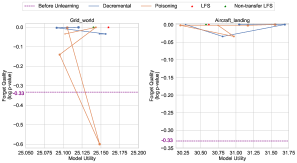
Figure 4. Forget Quality vs. Model Utility. Larger marker represents more unlearning epochs.

We compute the utility of the unlearned/retained model as the average cumulative rewards of it in the retaining environments. Figure 4 illustrates the trade-off between model utility and forget quality during unlearning in grid world and aircraft landing, where a larger marker denotes more unlearning epochs. In grid world (the left subfigure), the decremental RL-based method exhibits consistently high forget quality, while the poisoning-based method displays some fluctuations in forget quality but eventually attains a commendable level. This variance may be attributed to the randomness introduced by the RL algorithm in the poisoning-based approach. During the learning of the poisoning strategy, the method gradually converges, ultimately achieving a favorable result. Furthermore, both methods attain a higher forget quality than before unlearning, indicating the success of the unlearning process.

For model utility, both methods demonstrate robust performance, fluctuating in a narrow range of $(25.075,25.175)$. This performance is comparable to that of the retained models trained by the two baseline methods, i.e., learning-from-scratch (LFS) and Non-transfer LFS. A closer examination of model utility reveals a dynamic shift in utility in both methods as the unleanring progresses. This oscillation may arise from two factors. First, the decremental RL-based method aims to erase the agent’s knowledge, potentially leading to over-forgetting (Hu et al., 2024). Second, the poisoning-based method involves an intricate interplay between the RL dynamics and the strategic introduction of poison. This interplay can introduce randomness.

A similar trend is observed in aircraft landing (the right subfigure). The primary distinction is that the poisoning-based method exhibits fewer fluctuations in forget quality in aircraft landing compared to grid world. This discrepancy may be attributed to the less complex nature of the aircraft landing setting, allowing the poisoning strategy to converge more rapidly.

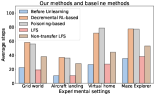
(a) Average steps of the four methods

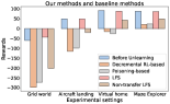
(b) Rewards of the four methods

Figure 5. Four methods in the unlearning environment

Next, we make detailed comparisons between our methods and the baselines. In Figure 5, it becomes evident that the unlearning results of the LFS baseline method in all four experimental settings are subpar. The agent’s performance in the unlearning environment remains nearly unchanged before and after unlearning. The reason for this result lies in the agent’s ability to generalize knowledge from other environments and apply it to the unlearning environment, despite never having encountered it before.

During training, the agent learns underlying rules and strategies from various environments. For instance, in the grid world setting, the agent acquires knowledge that obstacles should be avoided while collecting the target as quickly as possible. This learned knowledge, even if it was acquired in different environments, enables the agent to still perform well in unseen environments, including the unlearning environment. As a result, the baseline method proves to be ineffective as a reinforcement unlearning technique.

In contrast, the unlearning results of the Non-transfer LFS method surpass those of the regular LFS due to the limitation on its generalizability. Notably, Non-transfer LFS shows a considerable performance deterioration in the unlearning environment while maintaining effectiveness in other environments. These outcomes underscore the effectiveness of using an inverse loss function to minimize the agent’s cumulative reward in the unlearning environment.

4.3. Hyperparameter Study

Impact of Environment Size.  The alteration in the environment size allows us to evaluate how well the unlearning methods adapt and perform across different scales.

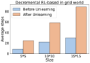
(a) Steps of decremental RL-based

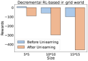
(b) Rewards of decremental RL-based

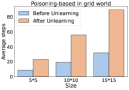
(c) Steps of poisoning-based

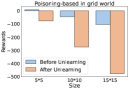
(d) Rewards of poisoning-based

Figure 6. The decremental RL-based and poisoning-based methods in Grid World with different sizes.

In the grid world setting, we extend the size of the environment from $5\times 5$ to $15\times 15$, resulting in a larger grid. Figure 6 visually depicts the impact of this increased environment size on both methods. As illustrated in the figure, we observe that with the expansion of the environment, the discrepancy in rewards between the pre-unlearning and post-unlearning stages is magnified for both methods. The reason is that the larger grid size introduces a greater number of states for the agent to navigate. Thus, unlearning becomes a more challenging task as the agent must modify its learned behavior to adapt to the enlarged environment. Also, this magnification effect can be attributed to the increased number of possible trajectories and interactions in the expanded grid world. After unlearning, the behavior of the agent in the unlearning environment becomes randomized. Consequently, a wider range of possible trajectories and interactions often leads to longer paths taken by the agent, thereby resulting in lower rewards attained. Hence, the discrepancy in rewards between the pre-unlearning and post-unlearning stages becomes more pronounced.

Impact of Poisoning Level.  The hyperparameter, poisoning level, serves as a pivotal factor in evaluating and testing the poisoning-based method exclusively. This parameter governs the quantity of poison introduced to the agent during the unlearning process, enabling us to investigate how the method performs under varying levels of poisoning. Specifically, the poisoning level is measured by the difference between the intended state $s^{\prime}$ and the manipulated state $\hat{s}^{\prime}$. To illustrate, in the grid world context where an agent’s state comprises eight dimensions, a poisoning level of 3 indicates that the two states differ in three dimensions.

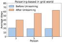
(a) Steps of poisoning-based

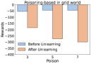
(b) Rewards of poisoning-based

Figure 7. The poisoning-based method in Grid World with different poison levels

Figure 7 illustrates the impact of changing the poisoning level on the evaluation metrics in the grid world setting. As the poisoning level increases, the values of all the evaluation metrics demonstrate a consistent downward trend. This trend indicates an improvement in the unlearning results with higher poisoning amounts. The reason behind this promising phenomenon lies in the nature of the poisoning-based method and its strategic use of targeted perturbations. As the poisoning level escalates, the method introduces a more substantial amount of deceptive information into the agent’s policy, causing a stronger deviation from the optimal path.

This increase in poisoning intensity effectively compels the agent to unlearn its previous behaviors more forcefully, encouraging it to abandon suboptimal policies. Thus, the agent’s learned policy becomes more adaptable and resilient, leading to enhanced performance in unlearning unwanted knowledge. Moreover, higher poisoning amounts facilitate a more efficient exploration of the policy space, allowing the agent to escape local optima and discover better solutions. Thus, the unlearning process becomes more effective in refining the agent’s behavior and enhancing its performance.

Consistent results across the remaining scenarios, illustrated in Figure 8 (aircraft landing), Figure 9 (virtual home), and Figure 10 (maze explorer), further strengthen the observations in the grid world setting. The increased poison during unlearning correlates with improved results. These findings emphasize the significance of the poisoning-based approach in reinforcement unlearning. By strategically introducing poison to prompt the agent to forget specific information, this method offers a promising solution for overcoming challenges in unlearning within complex environments.

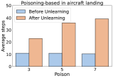
(a) Average steps of the poisoning-based method

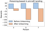
(b) Rewards of the poisoning-based method

Figure 8. The poisoning-based method in Aircraft Landing with different poison levels

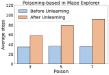
(a) Average steps of the poisoning-based method

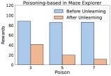
(b) Rewards of the poisoning-based method

Figure 9. The poisoning-based method in Virtual Home with different poison levels

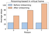
(a) Average steps of the poisoning-based method

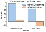
(b) Rewards of the poisoning-based method

Figure 10. The poisoning-based method in Maze Explorer with different poison levels

4.4. Adaptability Study

Dynamic Environments.  To illustrate the performance of our methods in dynamic environments, where the features and layouts of environments can change during agent training, we introduce a slight modification to the unlearning problem. Specifically, we consider an unlearning environment denoted as $\mathcal{M}_{u}$, and we employ time steps to represent changes in the environment. As time progresses in $t$ steps, the evolution of the unlearning environment can be represented as $\mathcal{M}^{1}_{u},\ldots,\mathcal{M}^{t}_{u}$. Thus, the problem of unlearning $\mathcal{M}_{u}$ transforms into the task of unlearning $\mathcal{M}^{1}_{u},\ldots,\mathcal{M}^{t}_{u}$.

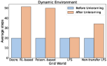
(a) Steps of the four methods

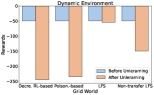
(b) Rewards of the four methods

Figure 11. Performance of the four methods in dynamic environments in Grid World

The experimental results, shown in Figure 11, were derived by setting $t=5$ and averaging the outcomes across the five environments. Similar outcomes can be observed for other values of $t$, e.g., $3$ and $8$. The results indicate that even in this dynamic setting, the outcomes of post-unlearning remain notably favorable. The effectiveness is attributed to the carefully designed mechanisms inherent in our reinforcement unlearning methods. Both unlearning methods involve dynamism during their operation. The decremental RL-based method dynamically adjusts the agent’s knowledge, ensuring it remains effective even as the environment undergoes alterations. Similarly, the poisoning-based method introduces dynamism by modifying the unlearning environment, ensuring the agent to perform optimally in the evolving environment.

Generalization.  To assess the generalization capability of our unlearning methods, we evaluated the unlearned models in unseen environments. We established the ratio between training environments and unseen environments as $4:1$, employing $20$ training environments and $5$ unseen environments. This configuration is analogous to the typical setting of the ratio between the size of the training set and the test set in conventional machine learning.

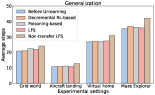
(a) Steps of the four methods

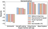
(b) Rewards of the four methods

Figure 12. Generalization of the four methods in Grid World

The outcomes, shown in Figure 12, were derived by averaging the results across the five unseen environments. The results indicate that the performance is sustained in these unseen settings. This suggests that our methods do not compromise the models’ generalization ability; instead, they selectively impact the models’ performance in the unlearning environments. This success can be attributed to the precision of our unlearning methods, which erase only the features specific to each unlearning environment while preserving the underlying rules gained from training environments.

Robustness.  Robustness gauges the strength and resilience of a method in the face of external perturbations. Evaluating robustness entails assessing how the unlearning methods perform when subjected to external perturbations. To conduct the evaluation, we introduce noise to the agent’s actions during both training and unlearning. The introduction of noise is achieved by randomly perturbing the probability distribution over the agent’s actions. This perturbation involves adding a small randomly generated number, falling within the range of $[-0.1,0.1]$, to a randomly selected probability in the distribution. This noise represents random variations or disturbances that can occur in real-world scenarios.

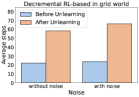
(a) Steps of decremental RL-based

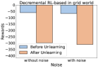
(b) Rewards of decremental RL-based

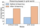
(c) Steps of poisoning-based

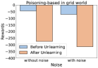
(d) Rewards of poisoning-based

Figure 13. The decremental RL-based and poisoning-based methods in Grid World with and without noise

The corresponding results of the grid world setting are presented in Figure 13. Upon analyzing the outcomes, a notable observation emerges: both the decremental reinforcement learning-based and poisoning-based methods exhibit remarkable robustness against external noise. Despite the introduction of noise, the difference in both steps and rewards between the pre-unlearning and post-unlearning states remains nearly unchanged for both methods. This robustness can be attributed to the inherent adaptability and resilience of the unlearning methods. In the case of the decremental RL-based method, the gradual modification of the agent’s policy allows it to withstand minor variations in observations, ensuring that its learned behavior remains stable despite external noise.

Similarly, the poisoning-based method’s strategic use of targeted perturbations enables the agent to develop a more adaptive policy. Thus, the agent’s behavior proves to be less affected by the noise, maintaining its consistency in unlearning undesired knowledge.

We have additionally assessed the unlearning process in two similar environments, delving into the consequences on one environment when unlearning the other. For adherence to page limitations, the detailed results are presented in the appendix.

4.5. Environment Inference Testing

This inference enables us to infer the environment that the agent needs to forget, allowing for a comparison of the inference outcomes before and after unlearning. In Figure 14, we present the results of the aircraft landing setting for the decremental RL-based method.

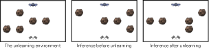
Figure 14. Inference results in Aircraft

The inference successfully recreates about $50\%$ of the unlearning environment before unlearning. However, after unlearning, this inference result significantly reduces to only $20\%$. This result provides clear evidence of a successful unlearning process. Note that the inference strategy employed in our experiments is not particularly effective. However, its use is solely for the purpose of illustrating the change in the percentage of an environment that can be inferred before and after unlearning. Evaluating our unlearning methods against a more potent inference strategy is left as future research.

The reason behind this success lies in the unlearning methods’ capability to modify the agent’s learned policy effectively. Both of the proposed methods adapt the agent’s behavior to forget specific aspects of the environment while preserving essential knowledge. Thus, the environment inference attack becomes less effective in recreating the forgotten parts after unlearning. Also, the visual comparison highlights the unlearning methods’ efficiency in refining the agent’s policy to eliminate unwanted behaviors. The process of inferring the forgotten environment confirms the success of our unlearning methods in reducing the agent’s reliance on previously learned information and adapting to changes in the environment.

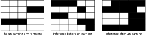
Figure 15. Inference results in Grid World

The results observed in the grid world scenario (Figure 15) are similar to the results in the aircraft landing setting, where the environment inference accuracy is significantly reduced after the unlearning process. In the grid world scenario, as the agent unlearns specific navigation patterns, the environment inference struggles to recreate the forgotten parts accurately. The unlearning process alters the agent’s policy, leading to changes in navigation trajectories. Thus, the inferred environment fails to capture the full complexity and intricacies of the original environment.

Note that these results not only show the accuracy of the inference but also exhibit the associated inference difficulty. A lower inference accuracy indicates a higher level of complexity in deducing information about an environment. It is essential to recognize that a diminished accuracy does not merely signify an error rate; rather, it implies that the inference process demands more time and effort to discern the intricacies of the environment accurately.

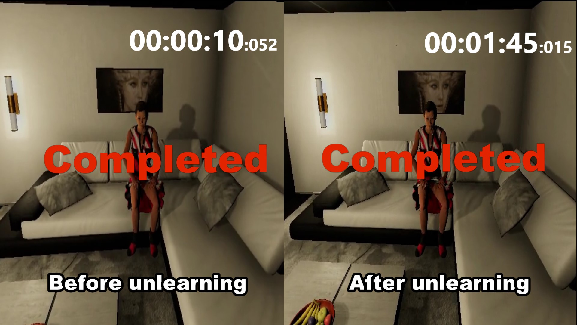
Figure 16. The time it took the agent to complete a predefined task before and after unlearning in Virtual Home

In the virtual home setting, where an environment inference is not applicable, we evaluated unlearning performance by measuring the time it took the agent to complete a predefined task before and after unlearning. As illustrated in Figure 16, before unlearning, the agent could swiftly complete the task in $10$ seconds. However, after unlearning, the agent needed $1$ minute and $45$ seconds to accomplish the same task in the same environment, showcasing its diminished performance resulting from the unlearning process.

5. Related Work

Machine Unlearning.  The concept of machine unlearning was initially introduced by Cao et al. (Cao and Yang, 2015). They employed statistical query learning and decomposed the model into a summation form, enabling efficient removal of a sample by subtracting the corresponding summand. Later, Bourtoule et al. (Bourtoule et al., 2021) proposed SISA training, which involves randomly partitioning the training set into multiple shards and training a constituent model for each shard. In the event of an unlearning request, the model provider only needs to retrain the corresponding shard model. Warnecke et al. (Warnecke et al., 2023) shifted the focus of unlearning research from removing samples to removing features and labels. Their approach is based on the concept of influence functions, which allows for estimating the influence of data on learning models. Machine unlearning has also been explored from a theoretical perspective. Ginart et al. (Ginart et al., 2019) introduced the concept of $(\epsilon,\delta)$-approximate unlearning, drawing inspiration from differential privacy (DP) (Dwork, 2006; Ruan et al., 2023; Feng et al., 2023). Subsequently, Guo et al. (Guo et al., 2020) formulated unlearning as certified removal and provided theoretical guarantees. They achieved certified removal by employing convex optimization followed by Gaussian perturbation on the loss function. Gupta et al. (Gupta et al., 2021) considered update sequences based on a function of the published model. They leveraged differential privacy and its connection to max information to develop a data deletion algorithm. Thudi et al. (Thudi et al., 2023) argued that unlearning cannot be proven solely by training the model on the unlearned data. They concluded that unlearning can only be defined at the level of the algorithms used for learning and unlearning.

Reinforcement Learning Security.  While reinforcement unlearning remains an underexplored area, considerable research has been devoted to reinforcement learning security. For instance, studies have extensively investigated the vulnerabilities present in RL systems (Wu et al., 2021) and policy explanation with security applications (Yu et al., 2023). However, it is crucial to note that these studies differ significantly from reinforcement unlearning for three distinct reasons. Firstly, the focus of prior research in reinforcement learning security primarily revolves around identifying and addressing vulnerabilities within the learning process. In contrast, our work centers on the fundamental task of how to effectively forget previously acquired knowledge. Secondly, existing studies in reinforcement learning security commonly aim to train robust agents capable of withstanding diverse adversarial activities. In contrast, our objective is to enable the unlearning of knowledge in a well-trained agent, highlighting a different goal and approach. Lastly, prior research endeavors to explain learned policies, particularly within security applications. In contrast, our research focuses on relearning policies based on revoke requests, giving a novel perspective on policy adaptation.

6. Conclusion

This paper presents a pioneering research area, termed reinforcement unlearning, which addresses the crucial need to protect the privacy of environment owners by enabling an agent to unlearn entire environments. We propose two distinct reinforcement unlearning methods: decremental RL-based and environment poisoning-based approaches. These methods are designed to be adaptable to different situations and provide effective mechanisms for unlearning. Also, we introduce a novel concept termed “environment inference” to evaluate the outcomes of the unlearning process. This evaluation framework allows us to assess the efficacy of our unlearning methods and gauge the level of privacy protection achieved in reinforcement learning-driven critical applications.

Appendix

Additional experimental results, along with details regarding the model architecture, are provided in this appendix.

1. Model Architecture

In the grid world and aircraft landing settings, we employ a fully-connected neural network as the model for our reinforcement learning agent. The neural network architecture consists of an input layer, two hidden layers, and an output layer. The input layer takes a 10-dimensional vector as input, representing the relevant features of the environment. The output layer generates a 4-dimensional vector, representing the probability distribution over the four possible actions: up, down, left, and right. The network architecture incorporates two hidden layers to facilitate learning and representation of complex patterns. The first hidden layer comprises 64 neurons, while the second one consists of 32 neurons.

In the virtual home and maze explorer settings, we employ a Convolutional Neural Network (CNN) comprising three CNN blocks and one hidden layer with 512 neurons. This network receives visual information as input with a size of $140\times 120$ and produces a 4-dimensional vector, indicating the probability distribution across the four possible actions: up, down, left, and right. The weights of these neural networks are randomly initialized.

2. Overall Performance

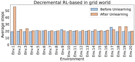
(a) The average number of steps before and after unlearning, where Environment 1 is the unlearning environment

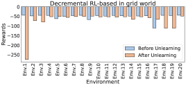
(b) The average rewards received by the agent before and after unlearning, where Environment 1 is the unlearning environment

Figure 17. The decremental RL-based method in Grid World

The presented experimental results were derived by averaging the outcomes across $100$ rounds of repeated experiments, and a $95\%$ confidence interval of $\textpm 3\%$ was calculated. The variances of the average reward and steps are both below 7 and 10, respectively. However, for clarity, they are not visually presented in the figures.

Figure 17 presents the overall performance of the decremental RL-based method in the grid world setting. The obtained results provide compelling evidence of the profound impact of the unlearning process on the agent’s performance, as evident from the average number of steps taken and the average received rewards metrics. Following unlearning, the agent demonstrates a substantial increase in the average number of steps taken and a notable reduction in the average received rewards compared to the pre-unlearning stage.

For example, in Figure 17(a), after unlearning, it is evident that the average number of steps taken by the agent in the unlearning environment substantially increases from $19.34$ to $55.8$, while in Figure 17(b), its reward decreases from $-44$ to $-273.5$. These findings indicate a significant performance reduction in the unlearning environment, which can be interpreted as a successful unlearning outcome. Conversely, in the retained environments, we observe minimal changes in the agent’s steps and rewards. This implies a successful preservation of performance in these environments.

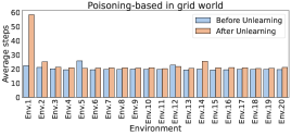
(a) The average number of steps before and after unlearning, where Environment 1 is the unlearning environment

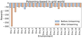
(b) The average rewards received by the agent before and after unlearning, where Environment 1 is the unlearning environment

Figure 18. The poisoning-based method in Grid World

Figure 18 presents the overall performance of the poisoning-based method in the grid world setting. It exhibits a similar trend to the decremental RL-based method. The reason for this similarity lies in the shared objective of both methods, which is to degrade the agent’s performance within the targeted unlearning environment while maintaining its performance in other environments. As a result, both methods effectively achieve the goal of reinforcement unlearning by selectively modifying the agent’s behavior within the specified context.

However, upon closer comparison between Figures 17 and 18, we can observe slight differences in the performance of the two methods in some remaining environments, such as Environments 18 and 19. In these environments, the poisoning-based method maintains almost unchanged steps and rewards between the pre-unlearning and post-unlearning stages, while the decremental reinforcement learning-based method does not achieve this. This result suggests that the decremental reinforcement learning-based method can potentially suffer from the over-unlearning issue to some extent, while the poisoning-based method demonstrates its ability to overcome this issue and retain better performance in the remaining environments after unlearning. These findings highlight the different characteristics and strengths of the two unlearning methods.

Figures 19, 20 and 21 demonstrate the overall performance of the decremental RL-based method in the context of aircraft landing, virtual home and maze explorer, respectively. In all the three scenarios, the agent’s behavior exhibits a notable increase in steps taken and a significant decrease in rewards achieved after the unlearning process. The reason for these trends in the three scenarios is rooted in the fundamental nature of reinforcement unlearning. The unlearning process seeks to selectively modify the agent’s behavior to forget specific environments or aspects of its learning history. Thus, the agent must re-explore and adapt to new circumstances, leading to fluctuations in its performance.

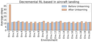
(a) The average number of steps before and after unlearning, where Environment 1 is the unlearning environment

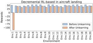
(b) The average rewards received by the agent before and after unlearning, where Environment 1 is the unlearning environment

Figure 19. The decremental RL-based method in Aircraft Landing

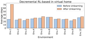
(a) The average number of steps before and after unlearning, where Environment 1 is the unlearning environment

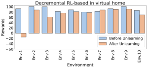
(b) The average rewards received by the agent before and after unlearning, where Environment 1 is the unlearning environment

Figure 20. The decremental RL-based method in Virtual Home

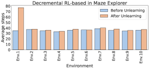
(a) The average number of steps before and after unlearning, where Environment 1 is the unlearning environment

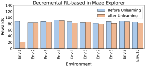
(b) The average rewards received by the agent before and after unlearning, where Environment 1 is the unlearning environment

Figure 21. The decremental RL-based method in Maze Explorer

Figures 22, 23 and 24 provide a comprehensive view of the poisoning-based method’s performance in the aircraft landing, virtual home and maze explorer settings, respectively. Remarkably, the performance trend in all the three scenarios is similar to that of the decremental RL-based method. This observation reinforces the effectiveness of the poisoning-based approach in reinforcement unlearning, as it consistently achieves the objective of degrading the agent’s performance in the targeted unlearning environment while preserving its capabilities in other environments. The consistent performance trend across different settings shows the method’s versatility and potential applicability in various RL scenarios.

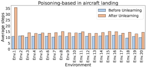
(a) The average number of steps before and after unlearning, where Environment 1 is the unlearning environment

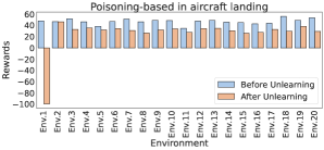
(b) The average rewards received by the agent before and after unlearning, where Environment 1 is the unlearning environment

Figure 22. The poisoning-based method in Aircraft Landing

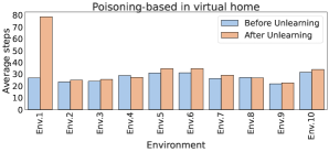
(a) The average number of steps before and after unlearning, where Environment 1 is the unlearning environment

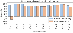
(b) The average rewards received by the agent before and after unlearning, where Environment 1 is the unlearning environment

Figure 23. The poisoning-based method in Virtual Home

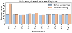
(a) The average number of steps before and after unlearning, where Environment 1 is the unlearning environment

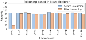
(b) The average rewards received by the agent before and after unlearning, where Environment 1 is the unlearning environment

Figure 24. The poisoning-based method in Maze Explorer

3. Hyperparameter Study

Impact of Environment Size. In the aircraft landing setting (Figure 25), the discrepancy in rewards between the pre-unlearning and post-unlearning stages becomes more pronounced for both the decremental RL-based and poisoning-based methods. Interestingly, this discrepancy in the aircraft landing setting is even larger compared to that observed in the grid world setting. The reason behind this distinction can be attributed to the inherent differences in the features and complexities of the two settings. In the grid world setting, the environment primarily consists of discrete and structured grids, with agent navigating through straightforward paths. The relatively limited environment complexity in the grid world setting allows the unlearning methods to efficiently adapt the agent’s behavior and modify its policy, resulting in significant yet manageable changes in rewards. On the other hand, the aircraft landing setting is considerably more intricate and continuous, involving multiple variables and parameters governing the aircraft’s landing procedures. As the size of the environment increases, the number of possible landing trajectories and configurations expands exponentially. This complexity poses a greater challenge to the unlearning methods, requiring them to navigate a more vast policy space.

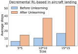
(a) Average steps of the decremental RL-based method

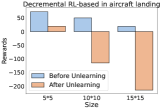
(b) Rewards of the decremental RL-based method

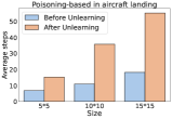
(c) Average steps of the poisoning-based method

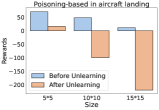
(d) Rewards of the poisoning-based method

Figure 25. The drecremental RL-based and poisoning-based methods in Aircraft Landing with different size

Impact of Environment Complexity. The complexity of an environment can be characterized by the presence and arrangement of obstacles within it. By modifying the complexity of the environment, we can assess the adaptability of the proposed methods. In the grid world setting, we examine the impact of increasing the environment complexity by introducing more obstacles, with the environment size maintained at $10\times 10$. Figures 26(a) and 26(b) show the outcomes of the decremental RL-based method.

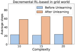
(a) Steps of decremental RL-based

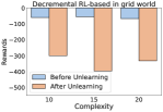
(b) Rewards of decremental RL-based

(c) Steps of poisoning-based

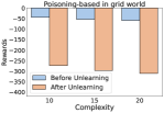
(d) Rewards of poisoning-based

Figure 26. The decremental RL-based and poisoning-based methods in Grid World with different complexity

We observe that as the number of obstacles is raised from $10$ to $15$, there is a notable increase in both the number of steps taken by the agent and the disparity in rewards between the pre-unlearning and post-unlearning stages. This observation suggests that with a moderate increase in complexity, the unlearning process becomes more challenging, resulting in a substantial alteration in the agent’s behavior, leading to changes in both step count and rewards. However, intriguingly, as we further augment the number of obstacles from $15$ to $20$, the difference in both steps and rewards between before and after unlearning seems to stabilize or vary less significantly. The reason behind this behavior lies in the agent’s learning adaptability. When the environment complexity rises from $10$ to $15$ obstacles, the agent faces substantial alterations in the optimal path and must undertake considerable unlearning to adjust its behavior accordingly. As a result, we observe a noticeable increase in step count and disparity in rewards. Conversely, when the number of obstacles increases from $15$ to $20$, the agent has already adapted its behavior to accommodate the increased complexity. As the agent’s policy has already been modified, further increases in obstacle count have a diminishing impact on step count and reward disparity.

However, when employing the poisoning-based method (depicted in Figures 26(c) and 26(d)), an interesting observation emerges. Unlike the decremental RL-based method, the difference in both steps and rewards between the pre-unlearning and post-unlearning stages remains relatively stable even as the number of obstacles increases. The reason behind this intriguing behavior lies in the nature of the poisoning-based approach. When we introduce additional obstacles to the environment, the poisoning-based method operates differently compared to the decremental RL-based approach. Instead of modifying the agent’s learned policy gradually, the poisoning-based method incorporates an element of targeted perturbation. As the number of obstacles increases, the poisoning-based method strategically poisons the agent’s policy by introducing deceptive information during the unlearning process. This targeted perturbation causes the agent’s behavior to deviate from the optimal path more significantly, leading to relatively constant differences in both step count and reward between the pre-unlearning and post-unlearning phases.

By undertaking a comparative analysis, it becomes evident that the poisoning-based method introduces a higher level of stability in performance compared to the decremental RL-based method. This enhanced stability is of significant interest and has several underlying reasons. Firstly, the poisoning-based approach leverages targeted perturbations to strategically poison the agent’s policy during the unlearning process. By introducing adversarial elements in a controlled manner, this method consistently influences the agent’s behavior, leading to more predictable changes in its performance.

Secondly, the poisoning-based method’s targeted perturbations are designed to cause deliberate deviations from the optimal path. As a result, the agent’s policy becomes consistently misled in the presence of additional obstacles, leading to a stable performance difference between the pre-unlearning and post-unlearning states.

Moreover, the consistent impact of the poisoning-based method can be advantageous in certain scenarios. For instance, in safety-critical environments, e.g., autonomous driving, where stability and predictability are crucial, the poisoning-based approach offers a more controlled and reliable means of unlearning unwanted behaviors. On the other hand, the decremental RL-based method, gradually modifying the agent’s policy, leads to more varied and less predictable changes in behavior as the environment complexity increases. This approach makes it challenging to precisely anticipate the agent’s performance changes in response to additional obstacles.

In Figure 27, the similar results observed in the context of aircraft landing corroborate the findings in the grid world setting. This outcome can be attributed to the analogous reasons previously identified in the grid world scenario.

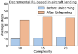
(a) Average steps of the decremental RL-based method

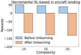
(b) Rewards of the decremental RL-based method

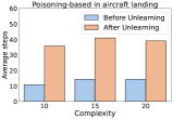
(c) Average steps of the poisoning-based method

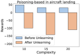
(d) Rewards of the poisoning-based method

Figure 27. The drecremental RL-based and poisoning-based methods in Aircraft Landing with different complexity

4. Adaptability Study

Similar Environments. In our evaluation, we intentionally introduced scenarios where two environments were very similar, with differences limited to just one grid in the grid world setting. The agent was then subjected to the unlearning process in one of these environments. After unlearning, we carefully examined the agent’s performance in the other environment.

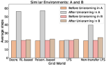
(a) Steps of the four methods

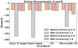
(b) Rewards of the four methods

Figure 28. The four methods in two similar environments, denoted as $A$ and $B$, in the grid world setting

The results of this experiment, shown in Figure 28, provide valuable insights. They demonstrate that when an agent undergoes unlearning in one of two similar environments, it does not exhibit deteriorated performance in the other environment. This finding supports the idea that the agent’s unlearning is environment-specific and does not extend to other environments, even if they are almost identical. This can be attributed to the characteristics of the two proposed unlearning methods. In the decremental reinforcement learning-based method, the agent is fine-tuned in the unlearning environment using a new loss function. In contrast, the poisoning-based method involves the agent’s retraining in a modified version of the unlearning environment. Consequently, even though the two environments are almost identical, the agent undergoes different training experiences, leading to distinct performance outcomes in the two environments. This outcome underscores the effectiveness of our reinforcement unlearning methods in achieving environment-specific knowledge removal while maintaining performance in other environments.

We have also undertaken the challenge of unlearning in both of the two similar environments. The outcomes, illustrated in Figure 29, reveal a deterioration in the agent’s performance across both environments. This observation underscores the profound impact of the unlearning process on the agent’s adaptability and proficiency in similar yet distinct environments. The discernible decline in performance serves as a compelling testament to the intricacies involved in unlearning an agent, shedding light on the nuanced dynamics that govern its responses in comparable scenarios.

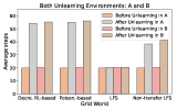
(a) Steps of the four methods

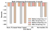
(b) Rewards of the four methods

Figure 29. The four methods in two similar environments, denoted as $A$ and $B$, in the grid world setting, when both environments are unlearned

We further investigated the scenario in which two environments are completely identical. However, the results revealed an intriguing outcome: after the agent undergoes the unlearning process in one environment, its performance in the identical counterpart deteriorates. Our hypothesis is that the agent’s updated knowledge, acquired during unlearning in one environment, is seamlessly applied to the identical environment, leading to a decline in performance. We leave the differentiation between two identical environments during reinforcement unlearning as our future research.

Robustness. The results observed in the aircraft landing (Figure 30), virtual home (Figure 31) and maze explorer (Figure 32) scenarios closely align with those in the grid world setting, showcasing the robustness of both the decremental reinforcement learning-based and poisoning-based methods against external noise. In the remaining three scenarios, the agent’s behavior continues to exhibit consistent patterns even when external noise is introduced during the unlearning process. This consistency is crucial for practical real-world applications, where agents must maintain their adaptability and performance despite uncertainties and disturbances. For example, in autonomous driving, noise from sensor readings or unexpected environmental conditions may often be encountered. The ability of the unlearning methods to maintain their efficacy despite such disturbances reinforces their practicality and reliability in dynamic environments.

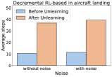
(a) Average steps of the decremental RL-based method

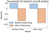
(b) Rewards of the decremental RL-based method

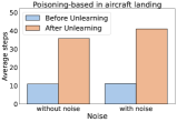
(c) Average steps of the poisoning-based method

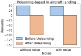
(d) Rewards of the poisoning-based method

Figure 30. The decremental RL-based and poisoning-based methods in Aircraft Landing with and without noise

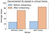
(a) Average steps of the decremental RL-based method

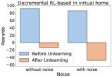
(b) Rewards of the decremental RL-based method

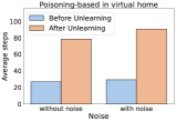
(c) Average steps of the poisoning-based method

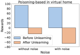
(d) Rewards of the poisoning-based method

Figure 31. The decremental RL-based and poisoning-based methods in Virtual Home with and without noise

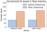
(a) Average steps of the decremental RL-based method

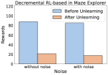
(b) Rewards of the decremental RL-based method

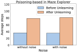
(c) Average steps of the poisoning-based method

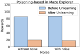
(d) Rewards of the poisoning-based method

Figure 32. The decremental RL-based and poisoning-based methods in Maze Explorer with and without noise

5. Numerical Results

In these numerical results, a new evaluation metric is adopted: trajectory similarity, which is defined as a sequence of state-action pairs. We evaluate the effectiveness of unlearning by comparing the similarity between two trajectories: one captured before unlearning and the other obtained after unlearning. Consider two trajectories, $\tau=((s_{1},a_{1}),\ldots,(s_{m},a_{m}))$ and $\tau^{\prime}=((s^{\prime}_{1},a^{\prime}_{1}),\ldots,(s^{\prime}_{m^{\prime}},a^{\prime}_{m^{\prime}}))$, where $\tau$ represents the trajectory recorded before unlearning, and $\tau^{\prime}$ corresponds to the trajectory collected after unlearning. The similarity between $\tau$ and $\tau^{\prime}$ is computed as:

(12) $$sim(\tau,\tau^{\prime})=\frac{\sum^{m}_{i=1}\mathbbm{1}_{s_{i}=s^{\prime}_{j}\wedge a_{i}=a^{\prime}_{j}}}{m},$$

where $\mathbbm{1}$ is the indicator function and $j$ is an index in $[1,m^{\prime}]$.

Table 1 numerically showcases the performance of the decremental RL-based method in the grid world setting with the size of $10\times 10$. An intriguing observation is the notable difference in trajectory similarity between the unlearning environment and the retained environments. In the unlearning environment, the trajectory similarity is as low as $35\%$, indicating that the unlearned policy operates substantially differently from the original policy in this specific environment. However, in the retained environments, the trajectory similarity remains around $85\%$ in average, implying that the unlearned policy only exhibits slight variations compared to the original policy. These results support the notion of successful unlearning, as the retained environments maintain a high level of performance similarity.

Table 1. Grid world $10\times 10$ under the decremental RL-based method, where Environment 1 is the unlearning environment

	Steps pre-unlearning	Steps post-unlearning	Reward pre-unlearning	Reward post-unlearning	Trajectory similarity
Environment 1	19.34	55.8	-44	-273.5	35%
Environment 2	$20.08$	$22.38$	$-47.8$	$-72.5$	$89\%$
Environment 3	$19.36$	$23.7$	$-44.6$	$-78.7$	$79\%$
Environment 4	$19.4$	$20.8$	$-45.1$	$-51.9$	$91\%$
Environment 5	$21.08$	$20.44$	$-62.2$	$-50.8$	$88\%$
Environment 6	$20.44$	$21.22$	$-50.8$	$-55.5$	$93\%$
Environment 7	$19.54$	$20.58$	$-45.9$	$-51.1$	$94\%$
Environment 8	$19.48$	$20.52$	$-44.6$	$-50.8$	$94\%$
Environment 9	$22.36$	$20.36$	$-66.8$	$-48.8$	$75\%$
Environment 10	$19.38$	$20.94$	$-46$	$-53$	$92\%$
Environment 11	$20.08$	$20.82$	$-48.5$	$-52.6$	$94\%$
Environment 12	$19.42$	$21.12$	$-45$	$-54.4$	$89\%$
Environment 13	$19.86$	$21.02$	$-47$	$-52.1$	$94\%$
Environment 14	$20.04$	$21.98$	$-48.9$	$-65.7$	$89\%$
Environment 15	$19.96$	$20.78$	$-48$	$-52.3$	$93\%$
Environment 16	$19.98$	$21.46$	$-47.3$	$-57.3$	$92\%$
Environment 17	$25.78$	$22.34$	$-110.5$	$-65.6$	$70\%$
Environment 18	$19.36$	$26.7$	$-44.7$	$-110.9$	$72\%$
Environment 19	$19.6$	$26.7$	$-45.9$	$-110.9$	$72\%$
Environment 20	$19.34$	$20.1$	$-44.1$	$-48.5$	$95\%$

The observation in the aircraft landing setting in Table 2 is similar to the grid world setting. The unlearning process successfully reduces the trajectory similarity in the unlearning environments, with values as low as $28\%$, while maintaining relatively high trajectory similarity around $90\%$ in average in the retained environments. These consistent results provide strong evidence of the effectiveness of our unlearning method in selectively modifying the agent’s behavior within the targeted unlearning environments while preserving its performance in other retained environments.

The results of the poisoning-based method align closely with those of the decremental RL-based method in the virtual home and maze explorer settings shown in Tables 3 and 4, respectively. The trajectory similarity is as low as $46\%$ and $35\%$ in the unlearning environment while maintaining high around $87\%$ and $84\%$ in average in the remaining environments in virtual home and maze explorer, respectively. This similarity can be attributed to the effectiveness of both methods in modifying the agent’s behavior within the targeted unlearning environments while preserving its performance in other retained environments. The poisoning-based method introduces deliberate changes to the state transition function of the unlearning environment, leading the agent to learn new, albeit incorrect, knowledge specific to the modified environment. Similarly, the decremental RL-based method selectively forgets learned knowledge related to the unlearning environment through iterative adjustments to the agent’s policy. As a result, both methods successfully enable the agent to adapt to the unlearning environment while maintaining its performance in other retained environments. The consistent performance across different settings showcases the robustness and efficacy of our reinforcement unlearning methods.

Table 2. Aircraft landing $10\times 10$ under the decremental RL-based method, where Environment 1 is the unlearning environment

	Steps pre-unlearning	Steps post-unlearning	Reward pre-unlearning	Reward post-unlearning	Trajectory similarity
Environment 1	10.72	36.9	50	-115	28%
Environment 2	$11.4$	$12.14$	$46$	$42.3$	$91\%$
Environment 3	$11.88$	$13.38$	$43.7$	$35.6$	$89\%$
Environment 4	$11.52$	$12.42$	$45.4$	$40.7$	$90\%$
Environment 5	$10.86$	$12.36$	$49.2$	$39.6$	$84\%$
Environment 6	$10.1$	$11.88$	$53.2$	$42.7$	$79\%$
Environment 7	$10$	$12.08$	$53$	$42.8$	$81\%$
Environment 8	$10.02$	$11.6$	$53.1$	$44.8$	$82\%$
Environment 9	$11.62$	$13.2$	$44.5$	$36.6$	$88\%$
Environment 10	$10.02$	$11.84$	$53.9$	$43$	$83\%$
Environment 11	$10.12$	$12.12$	$53.2$	$42.6$	$82\%$
Environment 12	$11$	$12.48$	$48.3$	$40.4$	$82\%$
Environment 13	$12.06$	$13.34$	$42.6$	$35.5$	$89\%$
Environment 14	$10.44$	$11.4$	$50.6$	$46.2$	$89\%$
Environment 15	$11.1$	$11.9$	$47.7$	$43.6$	$91\%$
Environment 16	$10.28$	$12.18$	$52.3$	$41.8$	$82\%$
Environment 17	$9.94$	$11.72$	$53.8$	$43$	$85\%$
Environment 18	$11.1$	$12.72$	$48$	$39.3$	$83\%$
Environment 19	$10.08$	$12.12$	$53.2$	$42.3$	$78\%$
Environment 20	$11.4$	$11.74$	$46.2$	$44.8$	$95\%$

Table 3. Virtual home under the poisoning-based method, where Environment 1 is the unlearning environment

	Steps pre-unlearning	Steps post-unlearning	Reward pre-unlearning	Reward post-unlearning	Trajectory similarity
Environment 1	26.34	55.6	92.88	6.48	46%
Environment 2	$23.42$	$25.02$	$102$	$94.3$	$86\%$
Environment 3	$23.76$	$24.02$	$90.56$	$87.36$	$94\%$
Environment 4	$28.28$	$30.48$	$80.44$	$82.48$	$89\%$
Environment 5	$31.5$	$32.3$	$76.28$	$72.6$	$90\%$
Environment 6	$33.38$	$35.04$	$74.2$	$70.6$	$93\%$
Environment 7	$27.06$	$26.96$	$89.56$	$92.16$	$99\%$
Environment 8	$27.84$	$31.64$	$91.28$	$80.72$	$85\%$
Environment 9	$21.28$	$22.8$	$100.16$	$94.16$	$87\%$
Environment 10	$32.28$	$32.2$	$80.88$	$81.8$	$96\%$

Table 4. Maze explorer under the poisoning-based method, where Environment 1 is the unlearning environment

	Steps pre-unlearning	Steps post-unlearning	Reward pre-unlearning	Reward post-unlearning	Trajectory similarity
Environment 1	35.2	77.3	88	21.2	35%
Environment 2	$37.2$	$37.9$	$83.6$	$83.4$	$86\%$
Environment 3	$34.9$	$36.1$	$87.51$	$85.47$	$80\%$
Environment 4	$33.1$	$33.9$	$91.6$	$90.1$	$84\%$
Environment 5	$35.9$	$37.7$	$86.81$	$81.75$	$80\%$
Environment 6	$36.4$	$36.3$	$83.9$	$85.1$	$90\%$
Environment 7	$38.9$	$40.1$	$81.7$	$79.67$	$87\%$
Environment 8	$35.7$	$38.1$	$87.15$	$81.1$	$79\%$
Environment 9	$34.5$	$35.5$	$89.2$	$86.5$	$82\%$
Environment 10	$36.1$	$37.2$	$85.47$	$82.6$	$85\%$

References

- (1)
- Artari (2023) Artari. 2023. https://paperswithcode.com/task/atari-games.
- Bourtoule et al. (2021) L. Bourtoule, V. Chandrasekaran, C. A. Choquette-Choo, H. Jia, A. Travers, B. Zhang, D. Lie, and N. Papernot. 2021. Machine Unlearning. In Proc. of IEEE S & P. 141–159.
- Cao and Yang (2015) Y. Cao and J. Yang. 2015. Towards Making Systems Forget with Machine Unlearning. In Proc. of IEEE S & P. 463–480.
- Dwork (2006) C. Dwork. 2006. Differential Privacy. In Proc. of International Conference on Automata, Languages and Programming. 1–12.
- Even-dar et al. (2004) E. Even-dar, S. M. Kakade, and Y. Mansour. 2004. Experts in a Markov Decision Process. In Proc. of NIPS.
- Fan et al. (2020) J. Fan, Z. Wang, Y. Xie, and Z. Yang. 2020. A Theoretical Analysis of Deep Q-Learning. https://arxiv.org/abs/1901.00137 (2020).
- Feng et al. (2023) C. Feng, N. Xu, W. Wen, P. Venkitasubramaniam, and C. Ding. 2023. Spectral-DP: Differentially Private Deep Learning through Spectral Perturbation and Filtering. In Proc. of IEEE S & P. 1944–1960.
- Garcelon et al. (2021) E. Garcelon, V. Perchet, C. Pike-Burke, and M. Pirotta. 2021. Local Differential Privacy for Regret Minimization in Reinforcement Learning. In Proc. of NIPS.
- GDPR (2016) GDPR. 2016. General Data Protection Regulation. https://gdpr-info.eu (2016).
- Ginart et al. (2019) A. A. Ginart, M. Y. Guan, G. Valiant, and J. Zou. 2019. Making AI Forget You: Data Deletion in Machine Learning. In Proc. of NIPS.
- Guo et al. (2020) C. Guo, T. Goldstein, A. Hannun, and L. van der Maaten. 2020. Certified Data Removal from Machine Learning Models. In Proc. of ICML.
- Gupta et al. (2021) V. Gupta, C. Jung, and S. Neel. 2021. Adaptive Machine Unlearning. In Proc. of NIPS.
- Gym (2023) Gym. 2023. https://gymnasium.farama.org.
- Harries et al. (2019) L Harries, S Lee, J Rzepecki, K Hofmann, and S Devlin. 2019. MazeExplorer: A Customisable 3D Benchmark for Assessing Generalisation in Reinforcement Learning. In Proc. of IEEE Conference on Games (CoG).
- Hu et al. (2024) Hongsheng Hu, Shuo Wang, Jiamin Chang, Haonan Zhong, Ruoxi Sun, Shuang Hao, Haojin Zhu, and Minhui Xue. 2024. A Duty to Forget, a Right to be Assured? Exposing Vulnerabilities in Machine Unlearning Services. NDSS (2024).
- Huang et al. (2017) D Y Huang, D Grundman, K Thomas, A Kumar, E Bursztein, K Levchenko, and A C Snoeren. 2017. Pinning Down Abuse on Google Maps. In Proc. of WWW. 1471–1479.
- Kirkpatrick and et al. (2017) J. Kirkpatrick and et al. 2017. Overcoming catastrophic forgetting in neural networks. PNAS 114, 13 (2017), 3521–3526.
- Kurmanji et al. (2023) M Kurmanji, P Triantafillou, J Hayes, and E Triantafillou. 2023. Towards Unbounded Machine Unlearning. In Proc. of NeurIPS.
- Lee et al. (2018) K Lee, S Kim, J Choi, and S Lee. 2018. Deep Reinforcement Learning in Continuous Action Spaces: a Case Study in the Game of Simulated Curling. In Proc. of ICML. 2937–2946.
- Lillicrap et al. (2016) T. P. Lillicrap, J. J. Hunt, A. Pritzel, N. Heess, T. Erez, Y. Tassa, D. Silver, and D. Wierstra. 2016. Continuous control with deep reinforcement learning. In Proc. of ICLR.
- Maini et al. (2024) P Maini, Z Feng, A Schwarzschild, Z C. Lipton, and J. Z Kolter. 2024. TOFU: A Task of Fictitious Unlearning for LLMs. https://arxiv.org/abs/2401.06121
- Massey Jr (1951) Frank J Massey Jr. 1951. The Kolmogorov-Smirnov test for goodness of fit. Journal of the American statistical Association 46, 253 (1951), 68–78.
- Mirowski et al. (2018) P Mirowski, M K Grimes, M Malinowski, K M Hermann, K Anderson, D Teplyashin, K Simonyan, K Kavukcuoglu, A Zisserman, and R Hadsell. 2018. Learning to Navigate in Cities Without a Map. In Proc. of NeurIPS.
- Mnih and et al. (2015) V. Mnih and et al. 2015. Human-level control through deep reinforcement learning. Nature 518 (2015), 529–533.
- Mnih et al. (2013) V. Mnih, K. Kavukcuoglu, D. Silver, A. Graves, I. Antonoglou, D. Wierstra, and M. Riedmiller. 2013. Playing Atari with Deep Reinforcement Learning. In Proc. of NIPS Deep Learning Workshop.
- Pan et al. (2019) X. Pan, W. Wang, X. Zhang, B. Li, J. Yi, and D. Song. 2019. How You Act Tells a Lot: Privacy-Leaking Attack on Deep Reinforcement Learning. In Proc. of AAMAS.
- Rakhsha et al. (2021) A. Rakhsha, G. Radanovic, R. Devidze, X. Zhu, and A. Singla. 2021. Policy Teaching in Reinforcement Learning via Environment Poisoning Attacks. Journal of Machine Learning Research 22 (2021), 1–45.
- Ruan et al. (2023) W. Ruan, M. Xu, W. Fang, L. Wang, L. Wang, and W. Han. 2023. Private, Efficient, and Accurate: Protecting Models Trained by Multi-party Learning with Differential Privacy. In Proc. of IEEE S & P. 1926–1943.
- Salem et al. (2023) A. Salem, G. Cherubin, D. Evans, B. Kopf, A. Paverd, A. Suri, S. Tople, and S. Z. Beguelin. 2023. SoK: Let the Privacy Games Begin! A Unified Treatment of Data Inference Privacy in Machine Learning. In Proc. of IEEE S & P. 327–345.
- Shi et al. (2021) G. Shi, J. Chen, W. Zhang, L. Zhan, and X. Wu. 2021. Overcoming Catastrophic Forgetting in Incremental Few-Shot Learning by Finding Flat Minima. In Proc. of NIPS.
- Shokri et al. (2017) R. Shokri, M. Stronati, C. Song, and Vi. Shmatikov. 2017. Membership Inference Attacks Against Machine Learning Models. In Proc. of IEEE S & P. 3–18.
- Thudi et al. (2023) A. Thudi, H. Jia, I. Shumailov, and N. Papernot. 2023. On the Necessity of Auditable Algorithmic Definitions for Machine Unlearning. In Proc. of USENIX Security.
- Tosatto et al. (2017) S. Tosatto, M. Pirotta, C. D’Eramo, and M. Restelli. 2017. Boosted Fitted Q-Iteration. In Proc. of ICML.
- Vietri et al. (2020) G. Vietri, B. Balle, A. Krishnamurthy, and S. Wu. 2020. Private Reinforcement Learning with PAC and Regret Guarantees. In Proc. of ICML.
- VirtualHome (2023) VirtualHome. 2023. http://virtual-home.org.
- Wang et al. (2022b) L Wang, S Xu, R Xu, X Wang, and Q Zhu. 2022b. Non-Transferable Learning: A New Approach for Model Ownership Verification and Applicability Authorization. In Proc. of ICLR.
- Wang et al. (2022a) X. Wang, S. Wang, X. Liang, D. Zhao, J. Huang, X. Xu, B. Dai, and Q. Miao. 2022a. Deep Reinforcement Learning: A Survey. IEEE Transactions on Neural Networks and Learning Systems (2022), DOI: 10.1109/TNNLS.2022.3207346.
- Warnecke et al. (2023) A. Warnecke, L. Pirch, C. Wressnegger, and K. Rieck. 2023. Machine Unlearning of Features and Labels. In Proc. of NDSS.
- Wu et al. (2021) X. Wu, W. Guo, H. Wei, and X. Xing. 2021. Adversarial Policy Training against Deep Reinforcement Learning. In Proc. of USENIX Security. 1883–1900.
- Xu et al. (2022) H. Xu, X. Qu, and Z. Rabinovich. 2022. Spiking Pitch Black: Poisoning an Unknown Environment to Attack Unknown Reinforcement Learning. In Proc. of AAMAS. 1409–1417.
- Xu et al. (2023) H. Xu, T. Zhu, L. Zhang, W. Zhou, and P. S. Yu. 2023. Machine Unlearning: A Survey. Comput. Surveys (2023). https://doi.org/10.1145/3603620
- Ye et al. (2022) J. Ye, A. Maddi, S. K. Murakonda, V. Bindschaedler, and R. Shokri. 2022. Enhanced Membership Inference Attacks against Machine Learning Models. In Proc. of CCS.
- Yu et al. (2023) J. Yu, W. Guo, Q. Qin, G. Wang, T. Wang, and X. Xing. 2023. AIRS: Explanation for Deep Reinforcement Learning based Security Applications. In Proc. of USENIX Security.
- Zhang et al. (2022) Z. Zhang, Y. Zhou, X. Zhao, T. Che, and L. Lyu. 2022. Prompt Certified Machine Unlearning with Randomized Gradient Smoothing and Quantization. In Proc. of NIPS.