Simultaneous ground-state cooling of two levitated nanoparticles by coherent scattering
Yi Xu
Key Laboratory of Low-Dimensional Quantum Structures and Quantum Control of Ministry of Education, Key Laboratory for Matter Microstructure and Function of Hunan Province, Department of Physics and Synergetic Innovation Center for Quantum Effects and Applications, Hunan Normal University, Changsha 410081, China
Yu-Hong Liu
Key Laboratory of Low-Dimensional Quantum Structures and Quantum Control of Ministry of Education, Key Laboratory for Matter Microstructure and Function of Hunan Province, Department of Physics and Synergetic Innovation Center for Quantum Effects and Applications, Hunan Normal University, Changsha 410081, China
Cheng Liu
Key Laboratory of Low-Dimensional Quantum Structures and Quantum Control of Ministry of Education, Key Laboratory for Matter Microstructure and Function of Hunan Province, Department of Physics and Synergetic Innovation Center for Quantum Effects and Applications, Hunan Normal University, Changsha 410081, China
Jie-Qiao Liao
Corresponding author: jqliao@hunnu.edu.cnKey Laboratory of Low-Dimensional Quantum Structures and Quantum Control of Ministry of Education, Key Laboratory for Matter Microstructure and Function of Hunan Province, Department of Physics and Synergetic Innovation Center for Quantum Effects and Applications, Hunan Normal University, Changsha 410081, China
Institute of Interdisciplinary Studies, Hunan Normal University, Changsha, 410081, China
Abstract
Simultaneous ground-state cooling of two levitated nanoparticles is a crucial prerequisite for investigation
of macroscopic quantum effects such as quantum entanglement and quantum correlation involving translational motion of particles. Here we consider a coupled
cavity-levitated-particle system and present a detailed derivation of its Hamiltonian. We find that the -direction motions of the two particles are decoupled from the cavity field and both the - and -direction motions, and that the -direction motions can be further decoupled from the cavity field and the -direction motions by choosing proper locations of the particles. We study the simultaneous cooling of these mechanical modes in both the three-mode and five-mode cavity-levitated optomechanical models. It is found that there exists the dark-mode effect when the two tweezers have the same powers, which suppress the simultaneous ground-state cooling. Nevertheless, the simultaneous ground-state cooling of these modes can be realized by breaking the dark-mode effect under proper parameters. Our system provides a
versatile platform to study quantum effects and applications in cavity-levitated optomechanical systems.
I Introduction
With the development of micro- and nano-fabrication techniques,
great advances have recently been achieved in cavity
optomechanics, especially on the fundamentals of quantum physics and modern quantum
technology Aspelmeyer2014 ; MAPR2014 . The optically levitated
particles, as a kind of novel optomechanical platform,
have attracted much attention from the communities of quantum optics and quantum information CSC2021 ; JRPP2020 ; Gaxv2307 .
In 1970s, it has been discovered that the particles can be levitated
by focusing beams of light Ask1 ; Ask2 ; Ask3 , and this discovery has
played a crucial role in advancing the field of atom trapping and cooling ARMP2009 . In recent years,
much attention has been paid to quantum manipulation of the translation and rotation of the center-of-mass
of particles, and great advances have been made in this platform, such as the realization of a controllable torque induced by the spins of atoms embedded in a microscale object TN2020 ,
the measurement of the Brownian motion of micrometer-sized beads TS2010 , and the cooling of the motion of particles into quantum ground state US2020 ; LN2021 ; FN2021 . The levitated particles can also be utilized for quantum precision measurements, including acceleration measurement FPRA2017 ; APRA2018 , mass measurement YPRL2020 , and gyroscope RPRL2018 ; JPRL2018 .
The levitated nanoparticles was conceived as a candidate to explore macroscopic
quantum phenomena PNAS2010 ; NJP2010 ; TLNP2011 ; APRL2010 ; JPRL2012 ; NPNAS2013 ; JNN2014 ; TNP2023 . This is because the nanoparticles are considered as a kind of macroscopic quantum system, and they can be levitated in a high vacuum NJP2010 ; PNAS2010 ; TLNP2011 ; Uaxv1902 , which reduces the
thermal contact between mechanical motion and environment. As a
result, these systems have exceptionally high mechanical quality factors, and are considered as an excellent candidate for studying low-dissipation optomechanics.
The first step to exploring quantum effects in macroscopic mechanical systems
is the cooling of the mechanical systems to their ground states IPRL2007 ; FPRL2007 ; JN2011 ; CPRL2019 ; LiuPRA2022 .
It has been reported that the levitated particles can be significantly cooled via feedback cooling TLNP2011 ; JPRL2012 ; APRL2010 ; RPRA2018 ; GPRL2019 ; FPRL2019
and sideband cooling PRA2010 ; PRA2011 ; PNC2013 ; JPRL2015 ; PPRL2016 ; APRR2022 .
The standard sideband-cooling method in optomechanical systems
typically requires an externally red-detuned pumping field to remove the energy from the particles NPNAS2013 ; NPRL1902 ; Uaxv1902 . However, high driving
powers will lead to the trapping of cavity fields for the optically levitated systems, and then reducing the cooling rate Uaxv1902 .
In addition, the laser-phase noise can hinder ground-state cooling at the relevant frequencies of the
trapped nanoparticles PPRA2009 ; ANJP2012 ; ANJP2013 . To overcome these challenges,
the coherent scattering technique has been introduced into the levitated particle
systems UPRL2019 ; DPRL2019 ; CPRA2019 ; US2020 ; JNP2023 , drawing from atomic physics experiments VPRL2000 . This method harnesses higher optical trapping powers and larger
particles to achieve stronger coupling strengths NC2021 , thereby paving the way to
ultra-strong coupling Kaxv2305 and leading to novel quantum optomechanical
effects. These works were mostly based on the cooling of a single particle.
In parallel, an increasing
amount of research is focusing on the field of multi-levitated particles CPRL2017 ; DQST2021 ; RPRL2021 ; YO2018 ; VO2021 ; TPRR2023 .
Compared with other mechanical oscillator arrays, the array of optically levitated particles has better controllability SA2020 ; JPR2023 ; CSC2023 ; YSC2023 .
Motivated by these advances, we are committed to study the simultaneously cooling multiple levitated particles and to explore more novel quantum effects.
In this paper, we study the simultaneous ground-state cooling of two levitated particles coupled to a cavity.
Similar to a single-particle case, the photon enters the cavity via the scattering
process, which provides the mechanism for cooling the center-of-mass motions of the particle. For multiple particles levitated simultaneously,
the mechanical effect of the scattered light between the particles has been ignored
in the past. However, the recent experimental observations indicate that this scattering effect cannot be neglected for some cases MPRL1989 ; VARB2006 ; KRMP2010 ; JS2022 . The redistributed light field greatly affects the
equilibrium position of the particles. Therefore, we consider the optical binding effect
between the two nanoparticles. In particular, we find that the -direction motions of the two particles decouple from other degrees of freedom in this system. We also find that, when the two nanoparticles are located at the cavity nodes,
the cavity mode only couples to the modes of the particles.
Benefiting from the extremal isolation of the system, the simultaneous ground-state cooling of the center-of-mass motions of the
two nanoparticles along -axis can be realized.
When the two nanoparticles are not located at the specific positions, both the mode
and the mode are coupled to the cavity mode, then the two modes of the two nanoparticles
can also be cooled into their ground states. In addition, we find that there exists the dark-mode
effect when the powers of the two tweezers are identical, and the dark-mode effect will
suppress the cooling of the system. By choosing proper parameters to avoid the dark-mode existing condition,
then the dark-mode effect can be broken, and the simultaneous ground-state cooling can be achieved.
The rest of the paper is organized as follows. In Sec. II,
we introduce the system consisting of two levitated nanoparticles trapped in a Fabry-Pérot cavity, and
analytically derive the Hamiltonians. In Sec. III,
we investigate the simultaneous ground-state cooling of the -direction motions of the two particles, which are located at the nodes of the cavity.
In Sec. IV, we study the simultaneous ground-state cooling of both the - and -direction motions of the two nanoparticles in a general case. Finally, we briefly conclude this work in Sec. V.
II Physical Model and Hamiltonians
We consider a coupled cavity-levitated-nanoparticle system, in which two dielectric nanoparticles trapped by two optical tweezers are coupled to the field modes in a Fabry-Pérot cavity.
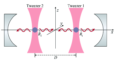
As shown in Fig. 1, the Fabry-Pérot cavity, with the cavity axis aligning with the direction, contains two nanoparticles. The two nanoparticles, placed at
and , have the radius nm, density kg/,
and dielectric constant . We assume that the two
optical tweezers have electric fields propagating along the axis, with the corresponding polarizations and along the direction. The foci of the two optical tweezers
are located at the positions and , separated by a distance . The frequency of the
two optical tweezers is ,
where is the speed of light in a vacuum and is the
wavelength of the tweezers.
Figure 1: Schematic of the physical setup. Two dielectric nanoparticles are
trapped at positions
and by two optical tweezers, where the cavity axis is along the direction, and the two optical tweezers propagate along the axis with polarization along the direction. The distance between the foci of the two tweezers is .
The total Hamiltonian of the system can be written as
(1)
Here, the Hamiltonian describes the kinetic energy of the center-of-mass
motion for the two nanoparticles, and it takes the form
(2)
where is the -dimensional momentum
operator for the th nanoparticle with mass . The second term in Eq. (1) reads
(3)
where and are, respectively, the electric and magnetical fields in the cavity, and is the free space premittivity (permeability). In addition, is the resonance frequency of the th cavity mode (described by the creation and annihilation operators and ) in the optical cavity.
Since the frequency of the center-of-mass motion for the nanoparticles
is much smaller than the free spectrum range of the cavity, we could consider that the two nanoparticles
are coupled to a single cavity mode. Then, the Hamiltonian of the optical cavity can be approximately denoted as , where is
the resonance frequency of the cavity mode under consideraion with the wave number , described by the creation and annihilation operators and . Note that the zero-point fluctuation term has been omitted in the Hamiltonian.
The last term in Eq. (1) describes the
interactions between the nanoparticles and the electromagnetic fields. In
the Rayleigh regime, the radius of the nanoparticle is much smaller than the
optical wavelength ( ), and the interaction Hamiltonian between the nanoparticles and the electric fields can be
written as UPRL2019 ; DPRL2019 ; CPRA2019
(4)
where is the particle polarizability with and being the volume of the nanoparticle. In Eq. (4), represents the electric field at the position of the th particle,
where denotes the center-of-mass position operator of
the th particle, with
being the focus of the th optical tweezer along the cavity axis
and the
position operator of the th particle.
II.1 The initial electric field
In general, the total electric field at the position can be approximately written as a sum of the
cavity field and the
fields for the two optical tweezers,
(5)
The first term in Eq. (5) describes the single-mode electric field of the cavity, which is given by
(6)
where is the amplitude at the center of the cavity with being the cavity volume. For simplicity, we consider the case and the -axis polarized cavity mode in this paper.
We assume that the two tweezers are sufficiently spaced apart such that the influence of the electric
field of tweezer 1 on the distant nanoparticle 2 can be neglected,
and vice versa. Then the total electric fields at the positions of the two nanoparticles 1 and 2 can be approximated as
(7a)
(7b)
Typically, the fields of the optical tweezers are considered in
coherent states and thus they can be well described by classical fields. Then the electric field of th optical tweezer can be expressed by
(8)
with the laser frequency and
wave number of the tweezer.
We assume that the propagating directions of two beams are parallel, and that
the polarizations and of the electric fields are along the direction. Then the real amplitude in Eq. (8) can be written as
(9)
where is the amplitude of the electric field, with being the power of the th laser and the tweezer waist at the focus. In addition, is the Rayleigh range and
. Note that the tweezer Gouy-phase in Eq. (8) can be neglected,
since the Rayleigh range is typically
several orders of magnitude larger than other length scales.
II.2 The radiation fields
In the Rayleigh regime, these nanoparticles embedded in the electric fields will
possess an electric dipole moment, which will create electromagnetic radiation
by charge oscillation. Physically, the frequency of the radiation field is equal to that of the
incident field. The electric field at position generated by the oscillating dipole at the position is given by
(10)
where the field propagator (also know as the dyadic Green’s function)
between the two dipoles is given by KRMP2010 ; Lbook2012 ; MPRA2018
(11)
Here, “T” denotes the matrix transpose, is the wave number of the incident field, is the distance between the two
dipoles, and . In the following analyses,
the Green function can be divided into two parts: Daxv2203 , where is the near-field constant and
is the far-field constant. The near-field constant is much smaller than the far-field constant in the far-field regime . In addition, we introduce the near-field tensor
(12)
and the far-field tensor
(13)
The total electric field for the th () particle is given by the sum of the
incident field and the field emitted by the other
dipole,
(14)
Here is the dipole moment generated by the th dielectric nanoparticle, where the index denotes the other particle with respect to the th particle (namely and ).
Since the cavity field and the tweezer field have
different wave numbers, the Green function will take two distinct forms,
and , corresponding to the wave numbers of the cavity field and the tweezer field, respectively. Consequently, the electric field can be divided into two parts, , with
(15a)
(15b)
Since the magnitude of is considerably small
compared to the trapping fields, we can neglect the second-order terms in Eq. (15). Then we
obtain the total electric field consisting of the incident field [the tweezer field and the cavity field ] and the emitted
field [ and ] by the dipole,
(16)
where describes the
radiation field generated by the oscillating dipoles at , which is induced by the th tweezer field . In addition, represents the radiation field produced by the dipole moment, which is
induced by the cavity field at the position .
II.3 The interaction Hamiltonians
In this section, we present the detailed expressions of the interaction Hamiltonians by putting the electric
field operator given by Eq. (16)
into Hamiltonians (4). The interaction Hamiltonian can be divided
into two parts , where the forms of the two parts are similar.
Below, we take the th (for =1,2) particle as an example. The Hamiltonian can be written as
(17)
which can be further divided into six terms
(18)
each of which represents a special physical interaction.
The first term in Eq. (18) is the standard interaction Hamiltonian of the cavity-field with the th
levitated particle
(19)
which consists of three parts .
Since the th particle is trapped near the focus of the th tweezer, we can
approximate the electric field of the tweezer by its expansion near . Then, we can obtain the harmonic potential energy of the tweezer as
with , where we employ the rotating-wave approximation
and neglect both the terms and the
constant terms. This means that the th nanoparticle is trapped by the tweezer with trapping frequencies .
The square term of the cavity field contains both the cavity frequecy shift and the radiation
pressure effect, , where and . In addition, the interaction term between the tweezer and cavity fields is given by , which describes
the displacement of the cavity mode and the coupling mediated by coherent scattering, where , , and .
The second term in Eq. (18) describes the
interaction between these radiation fields at position generated by the th oscillating dipole, and it is written as
(20)
We point out that the terms for are usually small enough to be ignored.
The remaining terms in Eq. (18) describe the interactions between the
incident field at the position of th particle and the field at
position generated by the th dipole. Concretely, these interaction Hamiltonians are given by
(21a)
(21b)
(21c)
(21d)
The four cross terms describe
the interactions between the incident field and the radiation field, and they
are generated by the mechanical effect of scattered light via the optical binding force. Equations (21a) and (21b) describe the
lateral binding and longitudinal binding, respectively. The optical binding force can be
calculated as KRMP2010 ; JS2022
(22)
where the force term describes the interaction between the emitted field
and the dipole at . Equation (21a) describes the interaction corresponding to the case where the two
particles are placed on the -axis, and they are trapped by the two
optical tweezers with the same frequency, respectively. Here, the two tweezers polarize along the -axis. In this
case, the binding force acting on particle 1 has the following components
(23a)
(23b)
(23c)
along the -, -, and -axes, respectively, with the distance between the two particles.
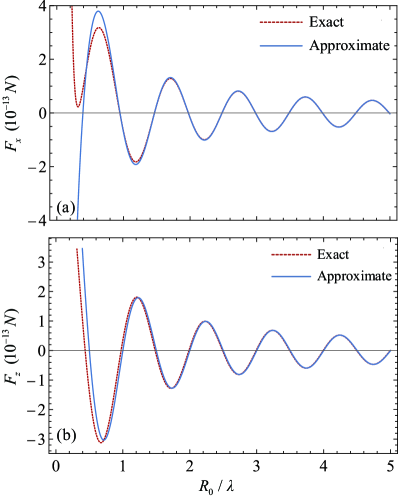
The Green function [Eq. (11)] contains these terms proportional to , , and . In the far-field region , the terms with dominate in the case, and then the Green function retains only the last term, i.e., . To investigate the specific scope of the far-field region , we compare in Fig. 2 the optical binding forces corresponding to the exact calculation and the far-field approximation. As shown in Fig. 2, we can find that the forces experience oscillations, and that as the scaled displacement increases, the oscillation amplitudes of the optical binding forces decrease. This oscillation behavior can be understood because the forces are functions of the trigonometric functions, as shown in Eqs. (23). Meanwhile, it can be seen from Fig. 2 that the exact optical-binding force is very close to the approximate optical-binding force when , which is consistent with the fact that the near-field constant is much smaller than the far-field constant when .
Figure 2: Comparison of the exact and approximate results concerning the optical binding forces (a) amd (b) (along -axis and -axis) between the two nanoparticles as
functions of the scaled distance . The radius of the two nanoparticles is nm, the numerical apertures of the two tweezers are , and the powers of the two tweezers are W and W.
Since these interaction terms described by Eqs. (21) involve two particles, below we analyze these cross interactions between the two particles together in the far-field regime.
The first cross term describes the lateral binding of the two
identical spherical nanoparticles. It is given by
(24)
where and correspond to the far-field constant and the far-field tensor for the wave number , respectively. Expanding the corresponding electric field near the foci of tweezers 1
and 2, the can be rewritten as
(25)
where the first term corresponds to a shift of the equilibrium position of the center-of-mass motion along -axis, and the displacement factor is given by
(26)
The second term in Eq. (25) describes the frequency shifts of the center-of-mass motion, with the frequency shifts
(27a)
(27b)
The third term in Eq. (25) describes the interaction between the two particles mediated by the light scattering, and the particle-particle coupling strengths are given by
(28a)
(28b)
(28c)
The second cross term given by Eq. (21b) represents the longitudinal binding of the two spherical
nanoparticles,
(29)
where and correspond to the far-field constant and the far-field tensor for the wave number , respectively. The Hamiltonian can be further re-expressed as
(30)
where the first term is the frequency shift term and the last two terms
are the optomechanical coupling terms, with the coupling strength
(31)
The third cross term describes the interaction between the th tweezer
field at and the field generated by the
other dipole caused by the cavity field. This term reads
(32)
which can be rewritten as
(33)
In Eq. (33), we introduced and the coupling strengths
(34a)
(34b)
(34c)
Finally, the interaction Hamiltonian between the cavity field and the field emitted by the
dipole induced by the tweezer fields reads
(35)
which can be further expressed as
(36)
Here, the displacement factor of mode is and the coupling strengths are
(37a)
(37b)
(37c)
Based on the above analyses, we obtain the total Hamiltonian in the rotating frame [defined by the unitary transformation operator ] as
(38)
where the effective driving detuning is with . The th particle exhibits a -mode frequency of with and , the displacement factor of the cavity mode and modes are, respectively, given by and , and the optomechanical couplings are given by and . It can be seen from Eq. (38) that the modes of the two
particles are only coupled to each other and decoupled from the other modes, so we
will only consider the and modes in the following discussions. We also note that, for concise, the hat for all the operators will be ignored in the following.
III Simultaneous ground-state cooling of the x-direction motions
For cooling of the -direction (along the cavity axis) motion of a single-levitated nanoparticle,
the best location of the particle is the nodes of the cavity mode UPRL2019 .
Below we consider that the two particles are located at and ,
which satisfy and . To cool the mechanical
modes, we consider the red-sideband resonance regime: . Concretely, we assume that the tweezer laser has the wavelength nm and the trapping
frequency of the particles is
MHz. Therefore, the driving frequency is much larger than the resonance
frequency of the oscillator , then the
wave number of the cavity field is approximately equal to that of the
tweezer field , and we can make the following
approximations: , , , , and . In this case, the Hamiltonian of the system is reduced to
(39)
where the -mode oscillation frequency of the th nanoparticle is given by , the coupling strengths are given by
(40a)
(40b)
and the displacement factor is
(41)
We see from Hamiltonian (39) that there exist bilinear couplings between the
cavity field and the -direction motions, the two harmonic oscillations are coupled with each other via the - interaction, and both the two oscillators are displaced in the -direction. For analyzing the cooling of the -direction motion, below we will
work in the displaced representation of the system such that the excitations are associated with the fluctuations.
For convenience, we introduce the dimensionless position and momentum operators and , where the zero-point motions are and . We also introduce the quadrature operators and for the cavity field.
Based on Eq. (39), we can obtain the quantum Langevin equations for the system as
(42a)
(42b)
(42c)
(42d)
(42e)
(42f)
where and are the decay rates of the cavity mode and the -direction motion of the th particle,
respectively. In Eqs. (42), we introduce , , and . The is the stochastic thermal noise
operator corresponding to the -mode motion of the th particle, which is determined by
the zero average values
(43)
and the correlation function,
(44)
where is the Boltzmann constant, and is the temperature of the thermal
bath associated with the mode. We assume that these mechanical modes
are connected to the high-temperature reservoirs (),
so we can obtain in the high-temperature limit. The stochastic noise is
reduced to a delta-correlation noise , where is the
thermal occupation number for the th thermal bath. In addition, the and are the optical noise operators, which
are determined by the zero average values and . The correlation functions of these optical noise operators are given by Cbook2000
(45a)
(45b)
(45c)
(45d)
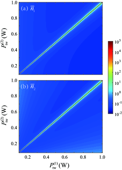
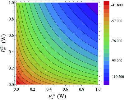
Figure 3: The final mean phonon numbers (a) and (b) in the two mechanical modes versus the powers and of the two tweezers. The
silica nanoparticle of radius is nm, the separation of
the particles is , the initial occupations are , and the effective driving detuning is . Other parameters used are and
To work in the displacement representation, we re-express Eqs. (42a)–(42f) around the steady-state values by writing
operators as the sum of average value
and quantum fluctuation: . Then, the Langevin equations can be separated into the semi-classical equations of
motion and the equations of motion for quantum fluctuations. The latter can be written as
(46a)
(46b)
(46c)
(46d)
(46e)
(46f)
By introducing the operator vector
(47)
and the noise operator vector
(48)
Eq. (46) can be expressed as a compact matrix form
(49)
where the coefficient matrix is given by
(50)
To calculate the final mean phonon numbers in these mechanical modes, we introduce the covariance matrix
defined by the matrix elements
(51)
for -. The covariance matrix is determined by the Lyapunov equation DPRL2007
(52)
where is the noise correlation matrix, defined by the elements for -.
Based on Eqs. (44) and (45), the noise correlation matrix can be obtained as
(53)
The final mean phonon numbers of the two mechanical modes can be
expressed as
(54)
where the stationary variance of the mechanical modes is given by the
corresponding diagonal matrix elements of the covariance matrix:
(55a)
(55b)
Therefore, the final mean phonon numbers in the two mechanical modes can be obtained by solving the Lyapunov equation.
In the coupled cavity-levitated-nanoparticles system, the powers of the optical tweezers affect both the resonance frequencies of the mechanical modes and the coupling strengths between the cavity mode and the mechanical modes. Below, we analyze the dependence of the cooling efficiency of the modes of the two nanoparticles
on the powers of the two optical tweezers. In Fig. 3, we plot the final mean
phonon numbers and as functions of the powers
and . We can see from Fig. 3 that the cooling of the two modes and is strongly suppressed when the two tweezers have the same powers. The cooling performance becomes better when the working point deviates the diagonal line . This phenomenon can be well
explained based on the dark-mode effect JNP2023 ; CNJP2008 ; DPRA2020 ; DPRL2022 ; JPRA2022a ; Jarx2023 .
From the expressions of and , we know that, when the powers of the two optical
tweezers are equal, i.e., , the two modes and have
the same resonance frequency , and the optomechanical coupling strengths are equal but with opposite signs .
In the following, we analyze the dark-mode effect in the system under these parameters.
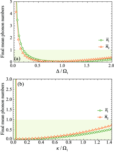
Figure 4: (a) The final mean phonon numbers (green solid line with circles) and
(yellow solid line with triangles) versus the scaled
driving detuning when . (b) The
final average phonon numbers and versus the scaled cavity linewidth at .
Other common parameters used are W, W, , .
Using the dimensionless operators, the Hamiltonian characterizing the quantum fluctuations can be written as
(56)
To clearly see the dark-mode effect in the system, we define two hybrid
modes of the two mechanical modes as
(57a)
(57b)
In the representation of the two new hybrid modes, the Hamiltonian can be expressed as
(58)
Figure 5: The particle-particle coupling strength versus
the powers and of the two optical tweezers.
Here, we take the following parameters: the radius of the two silica nanoparticles nm, the wavelength nm, and the numerical aperture .
where the resonance frequencies of the two hybrid modes are
(59)
In addition, the optomechanical coupling strength between the cavity mode and the
hybrid mode is given by , and the other two
coupling strengths between the two modes are given by
(60a)
(60b)
It can be seen from Eq. (58) that, when and ,
we have , and thus the mode is decoupled from both the mode and the cavity mode . In this case, the mode becomes a dark mode, and it cannot be cooled
via the cavity-field cooling channel. In
order to realize the simultaneous ground-state cooling of the two modes and , we can take different
optical tweezers powers, i.e., , then the dark-mode effect is broken.
In Fig. 4(a),
we plot the final mean phonon numbers and for the two mechanical modes
as functions of the scaled detuning in the nondegenerate-mechanical-mode case, .
In this case, we obtain the mechanical frequencies kHz for the center-of-mass motion
of the particle 1.
For this system, the nanoparticle is levitated in a vacuum, and hence it is highly isolated from the environment, resulting in a high -factor exceeding JNP2013 .
Under these parameters, the simultaneous ground-state cooling of the two mechanical modes can be realized . In particular, the optimal cooling of the mode for the th
particle appears around the red-sideband resonances: . Note that the slightly shifts of the resonance point are caused by the couplings among the optical modes and two mechanical modes. We point out that the present cooling scheme is essentially a sideband cooling. Therefore, we need to investigate the dependence of the cooling performance on the sideband resolution condition. To this end, we plot in Fig. 4(b) the final mean phonon numbers and as functions of the scaled cavity-field decay rate . Here we can see that the final mean phonon numbers and firstly decrease and then increase with the increase of the decay rate .
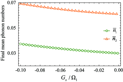
Figure 6: The final mean phonon numbers (green solid line with
circles) and (yellow solid line with triangles) as functions of
when and . Other parameters used are the same as those in Fig. 4
In this system, there exists a coupling between the two mechanical modes with the coupling strength .
Below, we investigate how does the coupling affect the cooling results of the two mechanical modes. Firstly, we point out that the particle-particle coupling strength used in Fig. 4 is , where the distance between the two particles.
It can be confirmed from Fig. 2 that the chosen parameters satisfy the far-field approximation well.
In addition, it can be seen from Eq. (28a) that the particle-particle coupling strength can be adjusted
by the powers and of the two tweezers and the distance
of the two particles.
To further elucidate this point, in Fig. 5 we plot the particle-particle coupling strength versus the powers and of the two tweezers. Figure 5 exhibits that the strength increases with the increase of the two powers and , which is consistent with the phenomenon that the optical binding force between the two levitated particles increases with the powers of the two tweezers. Moreover, we find can be adjusted from kHz to kHz and the scaled coupling .
In addition, the coupling strength is related to the size of the nanoparticles.
Since the particle-particle coupling provides a channel for the exchange of thermal excitations between the two mechanical modes and , it is interesting to analyze the dependence of the cooling results on the coupling strength . In Fig. 6, we plot the final mean phonon numbers and as functions of the scaled particle-particle coupling strength . Figure 6 shows that both the final mean phonon numbers and of
particles 1 and 2 increase with the increase of the absolute value of the particle-particle coupling ,
which means that the increase of the absolute value of the particle-particle coupling strength will
reduce the cooling efficiency of the two modes and .
IV Simultaneous cooling of x- and z-direction motions
In Sec. III, we considered the special case where the distance
between the two particles takes special values, resulting in the
decoupling of the cavity mode from the -direction motions of the two
particles. However, when the distance between the two particles does not take these
special positions, the cavity mode will couple to the -direction motions of the two particles. In the following, we will analyze
the cooling of both - and -direction motions of the two particles in this case.
For a general case, the system is described by Hamiltonian (38).
Here, there exist nonlinear coupling terms between the cavity mode and the -direction
motions of the two particles. In particular, we consider the case where the driving
[the term in Eq. (38)] of the cavity mode is strong enough, then we
can linearize the system and obtain the linearized Langevin equations as
(61)
Here the fluctuation operator vector is
(62)
where the mechanical quadratures are introduced as , , , and with . In Eq. (61), the noise operator vector is defined by
(63)
and the coefficient matrix is given by
(64)
In Eq. (64), we have defined ,
, and , then the linearized optomechanical-coupling strengths are given by
and . These complex coupling
strengths can be divided into real and imaginary parts, namely, and , where , , , and have been introduced in Eq. (64).
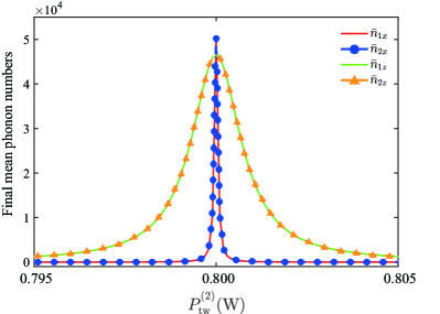
Figure 7: The final mean phonon numbers (red line),
(blue dashed line with dots), (green line), and (yellow dashed line with triangles) in
the four mechanical modes versus the power of the tweezer 2. Other parameters used are W, ,
, and .
These linearized coupling strengths depend on the semi-classical motion, which are governed by the semi-classical equations of motion.
In the steady-state case, the average values of the
system operators can be obtained as
(65a)
(65b)
(65c)
(65d)
(65e)
where and . Based on the linearized Langevin equations, we can derive an effective Hamiltonian as
(66)
where .
It can be seen from Eq. (66) that, the cavity mode is coupled to the four modes , , , and . Meanwhile, the modes and are coupled to the modes and , respectively. To investigate the dependence of the cooling performance of the four mechanical modes on the powers of the two tweezers, in Fig. 7, we plot the final mean phonon number , , , and as functions of when W.
Here, we can see that all the modes cannot be cooled around the identical power point . The phenomenon can be explained based on the dark-mode effect. In this five-mode system, when , we have and . Meanwhile, the coupling strengths satisfy the relations: , , and . To analyze the dark-mode effect, we introduce the creation and annihilation operators and of these mechanical modes. We further define four hybrid mechanical modes as
(67a)
(67b)
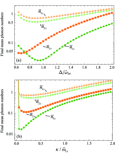
Figure 8: The final mean phonon numbers (green line with dots),
(orange line with squares), (light green dashed line with rhombuses), and (yellow dashed line with triangles) versus the effective driving detuning . Other parameters used are ,
, , , ,
, , , , and .
In the hybrid-mode representation, the Hamiltonian (66) can be re-expressed as a new form, which is not presented here because of its complicated form. By analyzing the Hamiltonian in the hybrid-mode representation, we find that the dark-mode effect appears under the conditions and . Accordingly, in the identical power case under consideration, the modes of the two particles have
the same frequency
and absolute value of coupling strength ,
and then the Hamiltonian is reduced to
(68)
where we have ignored the constant term. In Eq. (68), the normalized resonance frequencies are
and ,
and other parameters used are defined as , ,
, and . We can see from Eq. (68) that the two modes and are decoupled from other modes, and hence become the dark modes. Therefore, the cooling of the four mechanical modes will be significantly suppressed.
In order to break the dark-mode effect, we need to consider the
case , then we have and for our parameters. In the dark-mode-breaking case, we want to investigate the influence of the detuning on the cooling efficiency for these motions. In Fig. 8(a), we plot the final mean phonon numbers , , , and in the four mechanical modes versus the scaled detuning .
We find in Fig. 8(a) that the simultaneous ground-state cooling of the four mechanical
modes can be realized. In particular, the cooling performance of the -direction motions are better than those of the two modes and . Moreover, we can see from Fig. 8(a) that, for the two modes and , the optimal cooling appears respectively around and , corresponding to the red-sideband resonances. In this case, the effective mode temperatures of the -direction motions of the two nanoparticles are cooled to mK (corresponding to MHz), and the two -mode mechanical oscillators are simultaneously cooled to mK (corresponding to MHz). We also investigate the dependence of the final mean phonon numbers , , , and on the scaled decay rate for the cavity field, as shown by Fig. 8(b). Here, we can see that the simultaneous ground-state cooling of the four modes can be realized. In particular, the cooling performances of the two -direction modes and are better than those of the two -direction modes and . Meanwhile, we find that the main cooling region exists in the resolved-sideband regime.
V Conclusion
In conclusion, we have developed a theoretical model for
describing the simultaneous ground-state cooling of the motions of
two levitated nanoparticles trapped in a cavity via coherent scattering.
We have found that, different from the single-levitated particle case,
the scattered light will induce the mechanical effect between the
particles, which shifts the equilibrium position
of the particles and cause the coupling between two particles. We have derived the
Hamiltonian of the system and analyze the interactions in various cases. When the two nanoparticles are located at the nodes of the
cavity, the system is reduced to a three-mode loop-coupled model, in which the cavity mode is coupled to the -direction motional modes of the two particles, and the two modes are coupled with each other via the position-position coupling.
In this case, we have found that the dark-mode effect appears when two tweezers have
the same power, and then the effective cooling of the two mechanical oscillations is suppressed.
In particular, the simultaneous ground-state cooling of the -direction motion of the
two particles can be realized by breaking the dark-mode effect. In addition, when the particles are not
placed at the nodes, the system is reduced to a five-mode model, in which both the - and -direction motions are
coupled to the cavity mode, and there exist both the - coupling and - coupling between the two mechanical modes. In this case, we have also found that the dark-mode effect exists in the identical-power case, and that both the - and -direction motions can be significantly cooled by breaking the dark-mode effect.
This work paves the way to quantum manipulation of multiple levitated nanoparticles.
Acknowledgements.
J.-Q.L. was supported in part by National Natural Science Foundation of China (Grants No. 12175061, No. 12247105, and No. 11935006), the Science and Technology Innovation Program of Hunan Province (Grant No. 2021RC4029), and Hunan Provincial Major Science and Technology Program (Grant No. 2023ZJ1010).
References
(1) M. Aspelmeyer, T. J. Kippenberg, and F. Marquardt, Cavity optomechanics, Rev. Mod. Phys. 86, 1391 (2014).
(2) M. Metcalfe, Applications of Cavity Optomechanics, Appl. Phys. Rev. 1, 031105 (2014).
(3) J. Millen, T. S. Monteiro, R. Pettit, and A. N. Vamivakas, Optomechanics with levitated particles, Rep. Prog. Phys. 83, 026401 (2020).
(4) C. Gonzalez-Ballestero, M. Aspelmeyer, L. Novotny, R. Quidant, and O. Romero-Isart, Levitodynamics: Levitation and control of microscopic objects in vacuum, Science 374, eabg3027 (2021).
(5) G. Winstone, M. Bhattacharya, A. A. Geraci, T. Li, P. J. Pauzauskie, and N. Vamivakas, Levitated optomechanics: A tutorial and perspective, arXiv: 2307.11858.
(6) A. Ashkin, Acceleration and Trapping of Particles by Radiation Pressure, Phys. Rev. Lett. 24, 156 (1970).
(7) A. Ashkin and J. Dziedzic, Optical Levitation by Radiation Pressure, Appl. Phys. Lett. 19, 283 (1971).
(8) A. Ashkin, J. M. Dziedzic, J. E. Bjorkholm, and S. Chu, Observation of a single-beam gradient force optical trap for dielectric particles, Opt. Lett. 11, 288 (1986).
(9) W. D. Phillips, Nobel lecture: Laser cooling and trapping of neutral atoms, Rev. Mod. Phys. 70, 721 (1998).
(10) T. Delord, P. Huillery, L. Nicolas, and G. Hétet, Spin-cooling of the motion of a trapped diamond, Nature (London) 580, 56 (2020).
(11) T. Li, S. Kheifets, D. Medellin, and M. G. Raizen, Measurement of the instantaneous velocity of Brownian particle, Science 328, 1673 (2010).
(12) U. Delić, M. Reisenbauer, K. Dare, D. Grass, V. Vuletić, N. Kiesel, and M. Aspelmeyer, Cooling of a levitated nano-particle to the motional quantum ground state, Science 367, 892 (2020).
(13) L. Magrini, P. Rosenzweig, C. Bach, A. Deutschmann-Olek, S. G. Hofer, S. Hong, N. Kiesel, A. Kugi, and M. Aspelmeyer, Real-time optimal quantum control of mechanical motion at room temperature, Nature (London) 595, 373 (2021).
(14) F. Tebbenjohanns, M. L. Mattana, M. Rossi, M. Frimmer, and L. Novotny, Quantum control of a nanoparticle optically levitated in cryogenic free space, Nature (London) 595, 378 (2021).
(15) F. Monteiro, S. Ghosh, A. G. Fine, and D. C. Moore, Optical levitation of 10-ng spheres with nano- acceleration sensitivity, Phys. Rev. A 96, 063841 (2017).
(16) A. D. Rider, C. P. Blakemore, G. Gratta, and D. C. Moore, Single-beam dielectric-microsphere trapping with optical heterodyne detection, Phys. Rev. A 97, 013842 (2018).
(17) Y. Zheng, L.-M. Zhou, Y. Dong, C.-W. Qiu, X.-D. Chen, G.-C. Guo, and F.-W. Sun, Robust Optical-Levitation-Based Metrology of Nanoparticle’s Position and Mass, Phys. Rev. Lett. 124, 223603 (2020).
(18) R. Reimann, M. Doderer, E. Hebestreit, R. Diehl, M. Frimmer, D. Windey, F. Tebbenjohanns, and L. Novotny, GHz Rotation of an Optically Trapped Nanoparticle in Vacuum, Phys. Rev. Lett. 121, 033602 (2018).
(19) J. Ahn, Z. Xu, J. Bang, Y.-H. Deng, T. M. Hoang, Q. Han, R.-M. Ma, and T. Li, Optically Levitated Nanodumbbell Torsion Balance and GHz Nanomechanical Rotor, Phys. Rev. Lett. 121, 033603 (2018).
(20) D. E. Chang, C. A. Regal, S. B. Papp, D. J. Wilson, J. Ye, O. Painter, H. J. Kimble, and P. Zoller, Cavity opto-mechanics using an optically levitated nanosphere, Proc. Natl. Acad. Sci. U.S.A. 107, 1005 (2010).
(21) O. Romero-Isart, M. L. Juan, R. Quidant, and J. I. Cirac, Toward quantum superposition of living organisms, New J. Phys. 12, 033015 (2010).
(22) T. Li, S. Kheifets, and M. G. Raizen, Millikelvin cooling of an optically trapped microsphere in vacuum, Nat. Phys. 7, 527 (2011).
(23) A. A. Geraci, S. B. Papp, and J. Kitching, Short-Range Force Detection Using Optically Cooled Levitated Microspheres, Phys. Rev. Lett. 105, 101101 (2010).
(24) J. Gieseler, B. Deutsch, R. Quidant, and L. Novotny, Subkelvin Parametric Feedback Cooling of a Laser-Trapped Nanoparticle, Phys. Rev. Lett. 109, 103603 (2012).
(25) N. Kiesel, F. Blaser, U. Delić, D. Grass, R. Kaltenbaek, and M. Aspelmeyer, Cavity cooling of an optically levitated submicron particle, Proc. Natl. Acad. Sci. U.S.A. 110, 14180 (2013).
(26) J. Millen, T. Deesuwan, P. Barker, and J. Anders, Nanoscale temperature measurements using non-equilibrium Brownian dynamics of a levitated nanosphere, Nat. Nanotechnol. 9, 425 (2014).
(27) T. F. Kuang, R. Huang, W. Xiong, Y. L. Zuo, X. Han, F. Nori, C.-W. Qiu, H. Luo, H. Jing, and G. Z. Xiao, Nonlinear multi-frequency phonon lasers with active levitated optomechanics, Nat. Phys. 19, 414 (2023).
(28) U. Delić, D. Grass, M. Reisenbauer, T. Damm, M. Weitz, N. Kiesel, and M. Aspelmeyer, Levitated cavity optomechanics in high vacuum, Quantum Sci. Technol. 5, 025006 (2020).
(29) I. Wilson-Rae, N. Nooshi, W. Zwerger, and T. J. Kippenberg, Theory of Ground State Cooling of a Mechanical Oscillator Using Dynamical Backaction, Phys. Rev. Lett. 99, 093901 (2007).
(30) F. Marquardt, J. P. Chen, A. A. Clerk, and S. M. Girvin, Quantum Theory of Cavity-Assisted Sideband Cooling of Mechanical Motion, Phys. Rev. Lett. 99, 093902 (2007).
(31) J. Chan, T. P. M. Alegre, A. H. Safavi-Naeini, J. T. Hill, A. Krause, S. Gröblacher, M. Aspelmeyer, and O. Painter, Laser cooling of a nanomechanical oscillator into its quantum ground state, Nature (London) 478, 89 (2011).
(32) C. Sommer and C. Genes, Partial Optomechanical Refrigeration via Multimode Cold-Damping Feedback, Phys. Rev. Lett. 123, 203605 (2019).
(33) Y.-H. Liu, X.-L. Yin, J.-F. Huang, and J.-Q. Liao, Accelerated ground-state cooling of an optomechanical resonator via shortcuts to adiabaticity, Phys. Rev. A 105, 023504 (2022).
(34) R. Diehl, E. Hebestreit, R. Reimann, F. Tebbenjohanns, M. Frimmer, and L. Novotny, Optical levitation and feedback cooling of a nanoparticle at subwavelength distances from a membrane, Phys. Rev. A 98, 013851 (2018).
(35) G. P. Conangla, F. Ricci, M. T. Cuairan, A. W. Schell, N. Meyer, and R. Quidant, Optimal Feedback Cooling of a Charged Levitated Nanoparticle with Adaptive Control, Phys. Rev. Lett. 122, 223602 (2019).
(36) F. Tebbenjohanns, M. Frimmer, A. Militaru, V. Jain, and L. Novotny, Cold Damping of an Optically Levitated Nanoparticle to Microkelvin Temperatures, Phys. Rev. Lett. 122, 223601 (2019).
(37) P. F. Barker and M. N. Shneider, Cavity cooling of an optically trapped nanoparticle, Phys. Rev. A 81, 023826 (2010).
(38) O. Romero-Isart, A. C. Pflanzer, M. L. Juan, R. Quidant, N. Kiesel, M. Aspelmeyer, and J. I. Cirac, Optically levitating dielectrics in the quantum regime: Theory and protocols, Phys. Rev. A 83, 013803 (2011).
(39) P. Asenbaum, S. Kuhn, S. Nimmrichter, U. Sezer, and M. Arndt, Cavity cooling of free silicon nanoparticles in high vacuum, Nat. Commun. 4, 2743 (2013).
(40) J. Millen, P. Z. G. Fonseca, T. Mavrogordatos, T. S. Monteiro, and P. F. Barker, Cavity Cooling a Single Charged Levitated Nanosphere, Phys. Rev. Lett. 114, 123602 (2015).
(41) P. Z. G. Fonseca, E. B. Aranas, J. Millen, T. S. Monteiro, and P. F. Barker, Nonlinear Dynamics and Strong Cavity Cooling of Levitated Nanoparticles, Phys. Rev. Lett. 117, 173602 (2016).
(42) A. Ranfagni, K. Børkje, F. Marino, and F. Marin, Two-dimensional quantum motion of a levitated nanosphere, Phys. Rev. Research 4, 033051 (2022).
(43) N. Meyer, A. de los Ríos Sommer, P. Mestres, J. Gieseler, V. Jain, L. Novotny, and R. Quidant, Resolved-sideband cooling of a levitated nanoparticle in the presence of laser phase noise, Phys. Rev. Lett. 123, 153601 (2019).
(44) P. Rabl, C. Genes, K. Hammerer, and M. Aspelmeyer, Phase-noise induced limitations on cooling and coherent evolution in optomechanical systems, Phys. Rev. A 80, 063819 (2009).
(45) A. M. Jayich, J. C. Sankey, K. Børkje, D. Lee, C. Yang, M. Underwood, L. Childress, A. Petrenko, S. M. Girvin, and J. G. E. Harris, Cryogenic optomechanics with a Si3N4 membrane and classical laser noise, New J. Phys. 14, 115018 (2012).
(46) A. H. Safavi-Naeini, J. Chan, J. T. Hill, S. Gröblacher, H. Miao, Y. Chen, M. Aspelmeyer, and O. Painter, Laser noise in cavity-optomechanical cooling and thermometry, New J. Phys. 15, 035007 (2013).
(47) U. Delić, M. Reisenbauer, D. Grass, N. Kiesel, V. Vuletic, and M. Aspelmeyer, Cavity Cooling of a Levitated Nanosphere by Coherent Scattering, Phys. Rev. Lett. 122, 123602 (2019).
(48) D. Windey, C. Gonzalez-Ballestero, P . Maurer, L. Novotny, O. Romero-Isart, and R. Reimann, Cavity-Based 3D Cooling of a Levitated Nanoparticle via Coherent Scattering, Phys. Rev. Lett. 122, 123601 (2019).
(49) C. Gonzalez-Ballestero, P. Maurer, D. Windey, L. Novotny, R. Reimann, and O. Romero-Isart, Theory for cavity cooling of levitated nanoparticles via coherent scattering: Master equation approach, Phys. Rev. A 100, 013805 (2019).
(50) J. Piotrowski, D. Windey, J. Vijayan, C. Gonzalez-Ballestero, A. de los Ríos Sommer, N. Meyer, R. Quidant, O. Romero-Isart, R. Reimann, and L. Novotny, Simultaneous ground-state cooling of two mechanical modes of a levitated nanoparticle, Nat. Phys. 19, 1009 (2023).
(51) V. Vuletić and S. Chu, Laser Cooling of Atoms, Ions, or Molecules by Coherent Scattering, Phys. Rev. Lett. 84, 3787 (2000).
(52) A. de los Ríos Sommer, N. Meyer, and R. Quidant, Strong optomechanical coupling at room temperature by coherent scattering, Nat. Commun. 12, 276 (2021).
(53) K. Dare, J. J. Hansen, I. Coroli, A. Johnson, M. Aspelmeyer, and U. Delić, Linear Ultrastrong Optomechanical Interaction, arXiv:2305.16226.
(54) C. Marletto and V. Vedral, Gravitationally induced entanglement between two massive particles is sufficient evidence of quantum effects in gravity, Phys. Rev. Lett. 119, 240402 (2017).
(55) D. C. Moore and A. A. Geraci, Searching for new physics using optically levitated sensors, Quantum Sci. Technol. 6, 014008 (2021).
(56) R. Zhao, A. Manjavacas, F. J. García de Abajo, and J. B. Pendry, Rotational quantum friction, Phys. Rev. Lett. 109, 123604 (2012).
(57) Y. Arita, E. M. Wright, and K. Dholakia, Optical binding of two cooled micro-gyroscopes levitated in vacuum, Optica 5, 910 (2018).
(58) V. Svak, J. Flajšmanová, L. Chvátal, M. Šiler, A. Jonáš, J. Ježek, S. H. Simpson, P. Zemánek, and O. Brzobohatý, Stochastic dynamics of optically bound matter levitated in vacuum, Optica 8, 220 (2021).
(59) T. W. Penny, A. Pontin, and P. F. Barker, Sympathetic cooling and squeezing of two colevitated nanoparticles, Phys. Rev. Research 5, 013070 (2023).
(60) S. Liu, Z.-q. Yin, and T. Li, Prethermalization and nonreciprocal phonon transport in a levitated optomechanical array, Adv. Quantum Technol. 3, 1900099 (2020).
(61) J. Yan, X. Yu, Z. V. Han, T. Li, and J. Zhang, On-demand assembly of optically-levitated nanoparticle arrays in vacuum, Photon. Res. 11, 600 (2023).
(62) Y. Bao, S. S. Yu, L. Anderegg, E. Chae, W. Ketterle, K.-K. Ni, and J. M. Doyle, Dipolar spin-exchange and entanglement between molecules in an optical tweezer array, Science 382, 1138 (2023).
(63) C. M. Holland, Y. Lu, and L. W. Cheuk, On-demand entanglement of molecules in a reconfigurable optical tweezer array, Science 382, 1143 (2023).
(64) M. M. Burns, J.-M. Fournier, and J. A. Golovchenko, Optical binding, Phys. Rev. Lett. 63, 1233 (1989).
(65) V. Karásek, K. Dholakia, and P. Zemánek, Analysis of optical binding in one dimension, Appl. Phys. B 84, 149 (2006).
(66) K. Dholakia and P. Zemánek, Colloquium: Gripped by light: Optical binding, Rev. Mod. Phys. 82, 1767 (2010).
(67) J. Rieser, M. A. Ciampini, H. Rudolph, N. Kiesel, K. Hornberger, B. A. Stickler, M. Aspelmeyer, and U. Delić, Tunable light-induced dipole-dipole interaction between optically levitated nanoparticles, Science 377, 987 (2022).
(68) L. Novotny and B. Hecht, Principles of Nano-optics (Cambridge University Press, Cambridge, Eangland, 2012).
(69) M. A. Abbassi and K. Mehrany, Inclusion of the backaction term in the total optical force exerted upon rayleigh particles in nonresonant structures, Phys. Rev. A 98, 013806 (2018).
(70) D. De Bernardis, G. Rastelli, I. Carusotto, and V. Scarani, Optical-force-mediated coupling between levitated nanospheres can go ultrastrong, arXiv:2203.10126.
(71) C. W. Gardiner and P. Zoller, Quantum Noise (Springer, Berlin, 2000).
(72) D. Vitali, S. Gigan, A. Ferreira, H. R. Bohm, P. Tombesi, A. Guerreiro, V. Vedral, A. Zeilinger, and M. Aspelmeyer, Optomechanical Entanglement between a Movable Mirror and a Cavity Field, Phys. Rev. Lett. 98, 030405 (2007).
(73) C. Genes, D. Vitali, and P. Tombesi, Simultaneous cooling and entanglement of mechanical modes of amicromirror in an optical cavity, New J. Phys. 10, 095009 (2008).
(74) D.-G. Lai, J.-F. Huang, X.-L. Yin, B.-P. Hou, W. Li, D. Vitali, F. Nori, and J.-Q. Liao, Nonreciprocal ground-state cooling of multiple mechanical resonators, Phys. Rev. A 102, 011502(R) (2020).
(75) D.-G. Lai, J.-Q. Liao, A. Miranowicz, and F. Nori, Noise-Tolerant Optomechanical Entanglement Via Synthetic Magnetism, Phys. Rev. Lett. 129, 063602 (2022).
(76) J. Huang, D.-G. Lai, C. Liu, J.-F. Huang, F. Nori, and J.-Q. Liao, Multimode optomechanical cooling via general dark-mode control, Phys. Rev. A 106, 013526 (2022).
(77) J. Huang, C. Liu, X.-W. Xu, and J.-Q. Liao, Dark-Mode Theorems for Quantum Networks, arXiv:2312.06274.
(78) J. Gieseler, L. Novotny, and R. Quidant, Thermal nonlinearities in a nanomechanical oscillator, Nat. Phys. 9, 806 (2013).