ANN vs SNN: A case study for Neural Decoding in Implantable Brain-Machine Interfaces

Abstract

While it is important to make implantable brain-machine interfaces (iBMI) wireless to increase patient comfort and safety, the trend of increased channel count in recent neural probes poses a challenge due to the concomitant increase in the data rate. Extracting information from raw data at the source by using edge computing is a promising solution to this problem, with integrated intention decoders providing the best compression ratio. In this work, we compare different neural networks (NN) for motor decoding in terms of accuracy and implementation cost. We further show that combining traditional signal processing techniques with machine learning ones deliver surprisingly good performance even with simple NNs. Adding a block Bidirectional Bessel filter provided maximum gains of $\approx 0.05$, $0.04$ and $0.03$ in $R^{2}$ for ANN_3d, SNN_3D and ANN models, while the gains were lower ($\approx 0.02$ or less) for LSTM and SNN_streaming models. Increasing training data helped improve the $R^{2}$ of all models by $0.03-0.04$ indicating they have more capacity for future improvement. In general, LSTM and SNN_streaming models occupy the high and low ends of the pareto curves (for accuracy vs. memory/operations) respectively while SNN_3D and ANN_3D occupy intermediate positions. Our work presents state of the art results for this dataset and paves the way for decoder-integrated-implants of the future.

I Introduction

Implantable Brain-Machine Interfaces (iBMI) (Fig. 1(a)) are a promising class of assistive technology that enables the reading of a person’s intent to drive an actuator[1]. It holds promise to enable paralyzed patients to perform activities of daily living with partial or total autonomy[1]. While the first applications were in motor prostheses to control a cursor on a computer screen[2], or wheelchairs[3], or robotic arms[4], recent studies have shown remarkable results for speech decoding[5, 6], handwritten text generation[7] and therapies for other mental disorders[8].

The majority of clinical iBMI systems have a wired connection from the implant to the outside world [1]. However, this entails a risk of infection leading to the increasing interest in wireless neural interfaces [9, 1, 10]. Another trend in the field has been the continual increase in the number of electrodes[11] to increase the number of simultaneously recorded neurons (Fig. 1(b)) which can increase the accuracy of decoding user intent and enable dexterous control. Recently developed Neuropixels technology has pushed the number of recorded neurons to $\approx 1000$. However, this makes it a problem for wireless implants due to the conflicting requirements of high data rate and low power consumption[12]. Hence, there are efforts to compress the neural data on the sensor by extracting information from it by edge computing (Fig. 1(c)).

Different degrees of computing can be embedded in the implant ranging from spike detection, sorting to decoding[13]. Ideally, decoding on implant can provide the maximum compression [14] with the added benefit of patient privacy since the data does not need to leave the implant—only motor commands are sent out. Traditional decoders have used methods from statistical signal processing such as Kalman Filters and their variants[15]. With the rapid growth of Artificial Neural Networks (ANN) and variants for many different applications, it is natural to explore the usage of such techniques for motor decoding and several such works have recently been published [14, 16].

To fit on the implant, the decoder has to be extremely energy and area efficient along with being accurate. Brain-inspired SNN are supposed to be more energy-efficient due to their event-driven nature. They are also expected to be better at modeling signals with temporal dynamics due to their inherent “stateful” neurons with memory. However, detailed comparisons between SNN and ANN variants with controlled datasets and benchmarking procedures have been lacking. A recent effort[17] has put together a benchmarking suite to address this gap and one chosen task is that of motor decoding. We use the same dataset for benchmarking and show additional results for more control cases.

Neurobench showed that streaming SNNs provide a good tradeoff in terms of accuracy vs computes while other methods could have similar memory footprint. Further, it was shown that expanding traditional ANN with temporal memory (ANN-flat) at the input could drastically increase accuracy albeit at the cost of increased operations. Hence, we ask the question – will ANN models augmented with memory be better than SNNs in terms of the tradeoff between accuracy and cost (memory, operations/energy)? We make the following novel contributions in this paper:

• We compare SNNs with ANNs with memory augmentation at hidden state (by using LSTM) and output (by incorporating a traditional Bessel filter from signal processing).

• We show that combining NNs with traditional signal processing methods such as filtering drastically improves performance at minimial cost of additional operations or memory.

• We show the effect of increasing training data that shows which models have potential for improvements in future.

• We show the effect of testing with better curated data.

The rest of the paper is organized as follows. The following section discusses some of the related works while Section III describes the dataset, models and pre-processing used in this work. Section IV presents the results comparing different models in terms of their performance-cost tradeoff using pareto curves. This is followed by a section V that discusses the main results and provides additional control experiments. Finally, we summarize our findings and conclude in the last section.

Figure 1: (a) Conceptual figure of an iBMI that reads user intent and controls an effector. (b) Trend of exponential increase in the number of simultaneously recorded neurons[18]. (c) Integrating computing in the implant can reduce the wireless datarate enabling scalability of iBMI systems.

II Related Works and Contribution

The current work on designing decoders for motor prostheses can be divided into two broad categories–those using traditional signal processing methods and more recent ones based on machine learning.

II-A Traditional Signal Processing Decoders

An early decoder used in BMI system is the linear decoder, such as population vector (PV) algorithm [19]. Optimal linear estimators (OLE), generalized from PV algorithm, has comparable performance in closed-loop BMI systems, Whereas Bayesian algorithms perform better [20]. Inspired by estimation and communication theory, Wiener filter improved linear decoders by combining neuron history activation [21].

Kalman filter has an outstanding ability to cope with dynamic and uncertain environments and is suited in real-time applications. That makes Kalman filter one of the most widely used decoding algorithms in iBMI systems. However, the conventional Kalman filter is only optimal for linear variables and Gaussian noise [15]. Many variants of Kalman filter have been proposed to be applied to different applications or environments, such as decoding for cursor movement [15], predicting the movement for clinical devices [12], controlling the robotic arms [22], speech decoding [5].

II-B Machine Learning Decoders

Machine learning is widely used in various applications due to its powerful ability to process complex data. An SVM decoder could be trained to analyze rhythmic movements of Quadriplegia patients [23], or motor control of paralyzed limbs [24]. Recently, ANNs have attracted much attention among machine learning algorithms and have made great progress in BMI decoding. ELM-based intelligent intracortical BMI $($ $i^{2}$ BMI $)$ achieves an outstanding performance compared to traditional signal processing decoders [14]. A multi-layer ANN is trained to decode the finger movement running in a real-time BMI system, which outperforms a Kalman filter [16].

Recurrent neural networks (RNN) were introduced since they are more skilled at capturing the relations between two variables using a hidden state with memory. For instance, there have been studies on decoding speech [6] and on brain representation for handwriting [7]. Long-term decoding achieved higher performance by using LSTM and Wiener filter [25]. To decode speech for a paralyzed person, a natural-language model and Viterbi decoder are used [26].

Neuromorphic algorithms have emerged as an energy-efficient decoder and an effective tool for data compression [27]. SNN is a brain-inspired neural network popular in neuromorphic applications due to its low energy. It can achieve nearly the same accuracy as ANN but with less than $10\%$ memory access and computation of ANN [28]. Similarly, it was found that the SNN decoders could use far fewer computes compared to ANN, but with a performance penalty in accuracy, for the motor prediction of primates in the Neurobench benchmark suite[17].

In this work, we show that the combination of traditional signal processing and machine learning algorithms results in the best decoders for iBMI systems.

III Methodology

List of notations used in this section

• $N_{i}$: $i^{th}$ layer’s neuron count

• $N_{ch}$: No. of Input Probes

• $x_{i}$: Computed feature from i-th probe

• $T_{W}$: Bin window duration

• $m$: Number of sub-windows in a bin

• $St$: Stride size

• $s$: Sparsity

• $d$: Dropout rate

• $f_{GT}$: Ground truth label frequency ($=1/T_{GT}$)

III-A Dataset

The primate reaching dataset chosen for this paper was gathered and released by [29], with the six files chosen for Neurobench [17] being the files of interest. These six files are recordings of two non-human primates (NHP) (Indy and Loco), where each NHP accounts for three files (more details about this choice in [17]). This dataset contains microelectrode array (MEA) recordings of the NHP’s brain activity while it is moving a cursor to the target location, as seen in Figure 2. The finger velocity is sampled at $f_{GT}=250$ Hz resulting in ground truth labels at a fixed interval of $T_{GT}=4$ ms. The target position changes once the monkey successfully moves the cursor to the intended target. We refer to this action as a reach. The dataset contains a continuous stream of the brain’s activity from one MEA with $N_{ch}=96$ probes (Indy) or two MEAs with $N_{ch}=192$ probes (Loco). In this work, we ignore sorted spikes since it has been shown that spike detection provides sufficient information for decoding[30] and is more stable over time. Hence, the number of probes $N_{ch}$ is the input feature dimension $N_{0}$ for the neural network models (except ANN_3D) that will be discussed in the following subsection.

Training NN models on time series-based data requires the data to be split apart into separate segments. In analogy with keyword spotting[17], each segment of neural data should correspond to separate keywords. By using the target positions in this dataset, we can separate the spike data into segments based on indices in the target position array where there is a change in values, as illustrated in Figure 3. Such consecutive indices forms the beginning and end of a reach, and then we can split the time series into training, validation, and test sets based on the number of reaches. The split ratio used in this paper follows that of Neurobench[17], which is 50% for the training set, and 25% each for validation and test sets. The total number of reaches recorded in each file can be seen in Table I.

Figure 2: The experiment in the dataset has the NHP controlling the cursor and moving it to the target location. Once the NHP completes the action (referred to as a reach), the target location will move to a new location, and the subject will move the cursor accordingly.

(a)

(b)

Figure 3: How each reach is defined in this work: a) The start and end of a reach are marked by the index where there is a change in the target location array, indicating the monkey has moved the cursor to the previous target location. b) A sample segment taken from the file indy_20160622_01, where we can see five consecutive reaches being segmented.

TABLE I: Number of reaches in each file

Filename	Number of Reaches
indy_20160622_01	970
indy_20160630_01	1023
indy_20170131_02	635
loco_20170131_02	587
loco_20170215_02	409
loco_20170301_05	472

III-B Network Models

Figure 4: Architecture of models used in this paper are a) ANN b) ANN_3D c) SNN_3D d) SNN_Streaming and e) LSTM.

To explore the potential of various neural network models as the neural decoder, five different model architectures with and without memory are tested: ANN, ANN_3D, SNN_3D, Streaming SNN and LSTM, which can be seen in Figure 4. These five models use popular NN architectures and have memory at the input layer or hidden layer. Every model except for LSTM has two versions of varying complexity (explained in section IV-A) where complexity refers to the model size indicating the number of neurons. The larger model is henceforth referred to as the base model while the smaller model is dubbed the tiny variant. It was found that networks deeper than 3 layers performed poorly and hence deeper models were excluded from this study.

1. ANN or ANN_2D

   The ANN model has an architecture of $N_{ch}-N_{1}-N_{2}-2$, with rectified linear unit (ReLU) as the activation function for the first two-layers as well as batch normalization to improve upon the accuracy obtained by the model. Note that $N_{0}=N_{ch}$ indicates one feature extracted from each probe obtained by summing the neural spikes over a fixed duration of $T_{W}$ as described in Section III-C. Also, $N_{3}=2$ corresponds to predicting the $X$ and $Y$ velocities. A dropout layer with a dropout rate of $0.5$ is also added to the first two layers to help regularize the model. In analogy with the naming convention of ANN_3D introduced next, this model can also be referred to as ANN_2D due to the shape of the input weight tensor.

2. ANN_3D or ANN_flat

   The architecture of the ANN_3D or ANN_flat model is $m\times N_{ch}-N_{1}-N_{2}-2$, i.e. it shares an identical architecture with ANN, except at the input layer. This model divides the $T_{W}$ duration of the input bin window into $m$ sub-windows and creates a $m$-dimensional feature from each probe by summing spikes in each sub-window. This mode of input will be further explained in Section III-C. The input will then be flattened across the sub-windows, yielding a final input dimension of $N_{ch}\times m$; hence, the number of weights/synapses in the first layer is $m$ times more than ANN. It is referred to as ANN_flat in [17]; we refer to it as ANN_3D here in keeping with the shape of the input weight tensor, which we feel is more intuitive.

3. LSTM

   The LSTM model contains a single LSTM layer of dimension $N_{LSTM}$, followed by a fully-connected layer of dimension $2$. The input of the model shares the same pre-processor as ANN (summing spikes in a bin-window of duration $T_{W}$); however it uses a different $T_{W}$. The input is first normalized with a layer normalization, before passing through the rest of the network.

4. SNN_3D or SNN_flat

   The SNN_3D shares a similar architecture with ANN ($N_{ch}-N_{1}-N_{2}-2$), with the following differences: 1) Instead of using standard activation like ReLU, the SNN_3D model uses the leaky integrate-and-fire (LIF) neuron after every fully-connected layer, 2) the input is first passed through layer normalization, similar to LSTM due to the recurrent nature of LIF, and 3) at the final layer there is a scaling layer applied to the output LIF neurons. The LIF neurons are governed by the following set of equations:

   $$U[t] =\beta U[t-1]+WX[t]-S_{out}[t-1]\theta$$

   $$\beta =e^{-\Delta t/\tau}$$

   $$S_{out}[t] =\begin{cases}1&\text{if }U[t]>U_{thr}\\ 0&\text{otherwise }\end{cases}$$

   $$\theta =\begin{cases}0&\text{if no reset}\\ \beta U[t-1]+WX[t]&\text{if reset-to-zero}\\ U_{sub}&\text{if reset-by-subtraction}\end{cases}$$ (1)

   where $U[t]$ and $X[t]$ are the membrane potential of the LIF neuron and the input at the t-th time step respectively, $W$ is the synaptic weight of the fully-connected layer, $\beta$ is the decay rate, $S_{out}[t]$ is the output spike, $U_{thr}$ is the membrane potential threshold, $U_{sub}$ is the subtracted value if the reset mechanism is reset-by-subtraction and $\theta$ is the reset mechanism. The LIF neurons for all layers shares the same $U_{thr}$ and $\beta$. The first two layer uses the reset-to-zero mechanism while the last layer does not use any reset to allow the final output neurons to accumulate membrane potential to predict the velocity of the primate’s movement. For every stride of $4$ ms, the membrane voltages are reset and the integration is restarted with fresh input to produce the next output.

   The input for the SNN_3D model is different from ANN and identical to ANN_3D; however, unlike the ANN_3D model, the spike counts in the $m$ sub-windows spanning $T_{W}$ are input to the LIF neuron using only one weight/synapse but over $m$ time steps. Due to the reset of the LIF neurons after every prediction, overlapping bin-windows (for $T_{W}>st$) cause the SNN_3D to process the same input spikes for multiple predictions.

5. SNN_Streaming

   The SNN_Streaming model also consists of three fully-connected layers ($N_{ch}-N_{1}-N_{2}-2$), with LIF neurons (see Eq. 1) in each layer. Unlike SNN_3D, every LIF layer has its own unique $U_{thr}$ and $\beta$. Just like SNN_3D, the first two layer uses reset-to-zero while the last layer does not reset its membrane potential. In this model, $T_{W}=T_{GT}=St=4$ ms and hence does not require any additional pre-processing as seen in Section III-C; hence, it is called a streaming mode since inputs can stream in directly and continuously to this model.

III-C Input Spike Processing

(a)

(b)

(c)

Figure 5: Input data pre-processing methods presented in this paper: a) Summation mode, where the number of spikes detected within a bin window $T_{W}$ for each probe is summed to create a feature. b) Sub-window mode, where the bin window is further divided into $m$ sub-windows, and the number of spikes detected within each sub-window is summed. c) Streaming mode, where the input spike is gathered as it is.

The spikes generated by the NHP’s neurons are sparse in nature. While SNNs are designed with sparsity in mind, standard neural networks are not and hence require a feature extraction step from the raw spike data. Also, from the biological viewpoint, it is generally assumed that short term firing rates are important for motor control. Hence, we calculate firing rates, $r_{i}(t_{k})$ at the sample time $t_{k}$ from the spike waveforms $P_{i}=\sum_{t_{s,i}}\delta(t-t_{s,i})$ on the i-th probe ($1\leq i\leq N_{ch}$) using the following equation:

$$r_{i}(t_{k})=\int_{t_{k}-T_{W}}^{t_{k}}P_{i}(t)dt$$ (2)

where $t_{k+1}-t_{k}=T_{GT}$ is the sampling time, $t_{s,i}$ denote neural spike times on the i-th probe and $T_{W}$ is the bin window duration. Three different pre-processing methods were used in this paper: the summation method, the sub-window method and the streaming method as illustrated in Figure 5. For all of them, the stride size, $st$ is identical to the sampling duration, which is $T_{GT}=4$ ms. They differ in the choice of $T_{W}$ and how to present the firing information in the bin window to the network as described next.

1. Summation Method (used in ANN and LSTM):

   This is the simplest case where the firing rate in a bin window with duration of $T_{W}$ is directly used as a feature and input to the NN. We define the input feature vector $\overline{x}(t_{k})$ as follows:

   $$\overline{x}(t_{k}) =[x_{0}(t_{k}),x_{1}(t_{k}),...,x_{N_{ch}}(t_{k})]$$

   $$x_{i}(t_{k}) =r_{i}(t_{k})$$ (3)

   This method is depicted in Figure 5(a). This method is used by ANN and LSTM models, where ANN uses $T_{W}=200$ms while LSTM uses $T_{W}=32$ms. Efficient implementation of such firing rate calculation with overlapping windows are shown in [30].

2. Sub-Window Method (used in ANN_3D and SNN_3D):

   Similar to the summation method, the sub-window method uses information over the latest $T_{W}$ bin window. However, instead of summing all the spikes, it provides firing rate information at an even shorter time-scale (or with finer resolution) of $T_{W}/m$. Thus, the feature computed from the i-th probe itself becomes a vector $\overline{x_{i}}(t_{k})=[r_{i}^{1}(t_{k}),r_{i}^{2}(t_{k})...r_{i}^{m}(t_{k})]$ with $m$ components corresponding to firing rates in each of the $m$ sub-windows (duration of integration in Eq. 2 is reduced to $T_{W}/m$). The sub-window method is illustrated in Figure 5(b) and is used by the ANN_3D and SNN_3D models with $T_{W}=200$ms and $m=7$. The feature vector $\overline{x}(t_{k})$ for ANN_3D is defined according to Equation 4 as follows:

   $$\overline{x}(t_{k}) =[\overline{x_{0}}(t_{k}),\overline{x_{1}}(t_{k})..\overline{x_{N{ch}}}(t_{k})]$$ (4)

   where the dimension of $\overline{x}(t_{k})$ is $N_{ch}\times m$. For the SNN_3D, the firing rates in each sub-window are given as input feature to the SNN , which has $m$ time steps. Thus the input feature vector for the SNN in the j-th time step ($1\leq j\leq m$) is given by:

   $$\overline{x_{j}}(t_{k}) =[r_{j}^{1}(t_{k}),r_{j}^{2}(t_{k})...r_{j}^{N_{ch}}(t_{k})]$$ (5)

   where the dimension of $\overline{x_{j}}(t_{k})$ is $N_{ch}$. Note that ‘j’ indexes time steps here and the SNN output at $j=m$ is the prediction of motor velocity for sample time $t_{k}$.

3. Streaming Method (used in SNN_Streaming): The streaming method, as the name suggests, processes the incoming spike data as a continuous stream as seen in Figure 5(c). In this case, $T_{W}=st=T_{GT}=4$ ms implying no overlap between consecutive windows. This allows for a direct interface between the probes and the model, without the need of adding additional compute cost to our network like the two methods mentioned before. The input feature vector $\overline{x}(t_{k})$ is given by the following equation:

   $$\overline{x}(t_{k}) =[u(r_{0}(t_{k})),u(r_{1}(t_{k})),...u(r_{N_{ch}}(t_{k}))]$$ (6)

   where $u()$ denotes the Heaviside function. Hence, the resulting SNN can replace multiply and accumulate (MAC) operations by selective accumulation (AC) operations.

III-D Filter: Adding memory at output

Figure 6: Frequency distribution of ground truth and two model outputs from [17] for 2 sec of data from the fourth file in Table I shows higher frequency content in prediction. This indicates a strategy to choose filter cut off frequency.

Most of the NN models (with the exception of LSTM and SNN_Streaming) introduced in Section III-B operate on a window or chunk of inputs; providing these windows in any order would result in the same prediction. However, in real life the motor output is a smooth signal with a continuous trajectory. To understand this, we plot in Fig. 6 the frequency content of ground truth trajectories of a sample 2-sec waveform and compare it with predicted trajectories of two models from [17]. It is clear that the predictions have much higher frequency content indicating ground truth trajectories are smoother. In signal processing, this can be rectified by using a filter, which amounts to adding a memory of the past output. Among the different possible filters, a Bessel filter is chosen because of its linear phase response which is good for maintaining arbitrary waveform shapes. Three different filtering methods are tested in this work. First, we use forward (Fwd) filtering, which can achieve real-time filtering, but cannot be zero-phase. On the contrary, bidirectional (Bid) filtering can effectively eliminate phase distortions, but it is generally applicable to offline filtering since the whole waveform is needed before processing begins. To achieve a compromise, block bidirectional filter with a sliding window is applied, such that only a latency penalty of half window size is applicable. In this work, a window size of $16$ was chosen to limit the latency to $32$ ms while the order of filters and their cutoff frequencies were varied between $1-4$ and $0.05-0.5$ respectively to find the optimum for each model.

III-E Metrics

In order to evaluate the performance of the models comprehensively in terms of cost vs performance, three metrics are used: (1) number of operations, (2) memory footprint, and (3) accuracy. Three types of operations are considered for (1) – multiply, add and memory read (since the energy for memory access often dominates the energy for computations[31]). For most NNs, each synaptic operation comprises a multiply and add (MAC) while for SNN_Streaming, we only have additions (AC). The number of operations is used as proxy for power/energy in this work since the actual energy ratio between these three operations depends on bit-width, process node and memory size; more accurate energy evaluations will be the subject of future work. For (2), memory footprint is evaluated from model size where every parameter is stored using a 32-bit float number. For (3), R-Squared score is a commonly used metrics for regression tasks[15, 17, 14], which is defined by Equation 7:

$$R^{2}=1-\frac{{\textstyle\sum_{i=1}^{n}\left(y_{i}-\hat{y_{i}}\right)^{2}}}{{\textstyle\sum_{i=1}^{n}\left(y_{i}-\bar{y}\right)^{2}}}$$ (7)

where the label and predictions are showing as $y_{i}$ and $\hat{y_{i}}$ respectively while $\bar{y}$ is the mean of labels. For motor prediction, separate $R_{X}^{2}$ and $R_{Y}^{2}$ are computed for predicting X and Y velocities respectively and the final $R^{2}$ is an average of the two.

Another set of important metrics for NN hardware are throughput and latency. We have not considered them here since the considered NN models are small enough so that the total time taken for evaluating the prediction is dominated by the input data accumulation time shown in Section III-C. However, we do touch upon this point later in Section V.

III-F Training & Testing Details

All models are trained for $50$ epochs using the SNNTorch framework, with a learning rate of $0.005$, a dropout rate between $0.3-0.5$, and an L2-regularization value between $0.005-0.2$. AdamW is chosen as the optimizer, Mean Squared Error (MSE) loss is determined as the loss function, and a learning scheduler (cosine annealing schedule) is used after every epoch. For ANN, ANN_3D, and SNN_3D, data is shuffled with batch size of $512$ in training. For SNN_3D, the membrane potential resets every batch, while reset occurs at the beginning of each reach for membrane potential in SNN_streaming and hidden states in LSTM. The distribution of reach dutrations show most reaches completed in less than $4$ sec while some reaches being much longer, presumably due to the NHP not attending to the task. Similar to [17], reaches that exceed $8$ seconds in length are removed to improve the training performance. Leaky Integrate-and-Fire Neuron is used in SNNs, where the threshold and $\beta$ are learned during training and Arctan is applied as a surrogate function. The membrane potential of neurons ceases to reset in the last layer to enable regression. The velocity predicted by SNNs is determined by scaling the membrane potential of neurons with a learnable constant parameter. For validation and testing, data is input to the models in chronological order, and reset mechanisms only occur at the beginning. Filters are employed exclusively during the inference process.

IV Results

To comprehensively examine the capability of different models, we performed multiple experiments and evaluated models using the metrics mentioned in Section III-E. All the results except memory access are obtained from the neurobench harness[17] that does automated evaluation of the models; memory access is estimated based on theoretical equations of weight fetches based on experimentally observed sparsity multiplying the number of weights on a per layer basis. The findings are presented pictorially using two pareto plots, first comparing the accuracy versus operations trade-off and the second comparing accuracy versus memory footprint (e.g. see Figures 8 and 10). For the pareto plots shown in this section, the following colour scheme is used:

• blue markers are base models without filtering (correspond to results from prior work in [17] for ANN, ANN_3D and SNN_3D)

• red markers are models using forward (Fwd) filtering

• green markers are models using bidirectional (Bid) filtering

• orange markers are models using block Bid filtering

• markers with dark border are tiny variants of base models

A tabular summary of all the experiments performed for our base models can be found in Table III.

IV-A Model Size Search

As mentioned earlier, it was found that networks deeper than 3 layers performed poorly and hence deeper models were excluded from this study. The number of neurons in each of the two hidden layers was determined by searching within a certain range ($N_{0}=N_{ch}$ and $N_{3}=2$ are fixed). We used the ANN to do this search due to its simplest network structure and resultant fast training. Each model complexity is characterized by the number of neurons. The results obtained by varying $N_{1}$ and $N_{2}$ are shown in the Figure 7. The text shown in the figure represents the different network architectures ($N_{1}-N_{2}$ combinations) tested. As expected, the $R^{2}$ initially increases with increasing number of neurons but starts decreasing after the number of neurons reaches a certain value due to overfitting. The best trade-off between $R^{2}$ and complexity is determined by the networks lying on the pareto curve. Therefore, the two models with $N_{1}-N_{2}$ values of $32-48$ and $16-32$ were selected as the ‘base’ and ‘tiny’ variants respectively for ANN. Same variant sizes were near optimal for ANN_3D and SNN_3D (we do not show these tradeoff curves for brevity), while for SNN_Streaming, base and tiny variants represented $N_{1}-N_{2}$ values of $32-48$ and $16-48$ respectively.

Figure 7: Complexity versus $R^{2}$ for different ANN models tested. $N_{1}-N_{2}$ values of $16-32$ and $32-48$ were on the pareto curve and chosen as ‘tiny’ and ‘baseline’ variants.

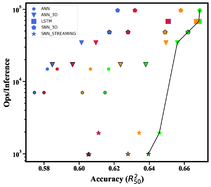
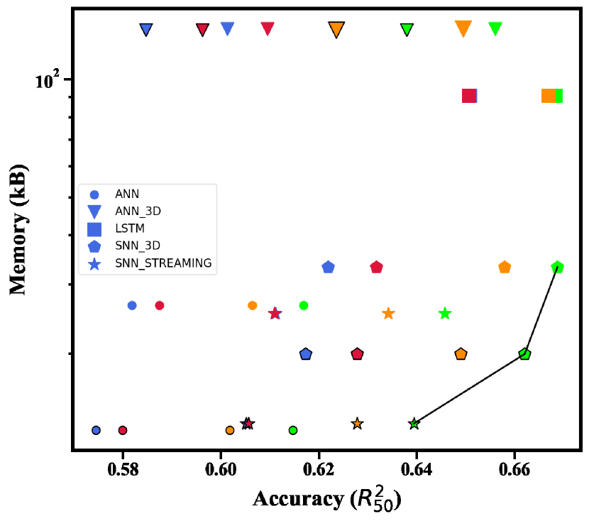
Figure 8: Baseline Pareto plots showing trade-offs for different models: a) Compute cost vs. accuracy b) Memory footprint vs. accuracy

IV-B K-Fold Cross Validation

It is important to verify that the result will not vary significantly regardless of how the data is split. Hence, K-fold cross-validation is used to test all six files for three models (ANN, ANN_3D and SNN_3D). We divided the data into five parts, randomly selecting four parts as training and the other part was divided into validation and testing. The means and standard deviations of $R^{2}$ for the 5-fold experiment are shown in Table II. Low variance of the results for all 3 cases implies using one-fold data split for our experiment is reasonable and will give dependable results. As a comparison, the results in Table III does show that without filter, the decoding accuracy for SNN_3D is the best and ANN is the worst with ANN_3D between the two. Hence, we just use the single data split in [17] described earlier for the rest of the results.

TABLE II: K-fold Cross Validation

Models	$R^{2}$ Mean	$R^{2}$ Standard Deviation
ANN	0.6186	0.0294
ANN_3D	0.6467	0.0299
SNN_3D	0.6661	0.0252

IV-C Baseline result and effect of filtering

The pareto plots showing the baseline comparison can be seen in Figure 8. The filter order and cutoff frequency are chosen separately for different filtering methods and different models. For ANN, ANN_3D, SNN_3D and SNN_Streaming, filter order and cutoff frequency are $4$ and $0.05$ for bidirectional filtering, while in block bid filtering, order is selected as $2$. For forward filtering, the parameters are $1$ and $0.15$ for order and cutoff frequency respectively. However, these are different in LSTM and set at $2$ and $0.07$ for order and cutoff for all kinds of filtering methods. These optimal parameters were selected based on results in the validation set by doing a grid search over filter orders $1-4$ and cut-off frequencies in the range $0.05-0.5$ as mentioned earlier in Section III-D.

In terms of the models that forms the pareto front of operations vs. accuracy (Fig. 8(a)), we observe all of them use bidirectional filtering to achieve their high accuracy. While this is impractical in real-time decoding, these results can be taken as a gold standard for the neurobench suite at this time since they represent the highest reported accuracy so far. Along the pareto front, the two SNN variants, SNN_3D and SNN_Streaming show the biggest difference in terms of operations required ($\approx 100$x) and accuracies ($\approx 0.022$), while LSTM and ANN_3D are at intermediate positions on the pareto front. In terms of memory usage (Fig. 8(b)), the pareto front is dominated by SNNs of the two types. The ANN_3D models have highest memory usage due to their input dimension being expanded by $m$ times to $m\times N_{ch}$–the weights in the first layer are dominant for memory footprint since $N_{0}>>N_{1},N_{2},N_{3}$.

If we ignore models with Bid filtering due to them not being applicable in real-time, the next pareto frontier is dominated by models with block BiD filtering. Both these results point to the extreme efficiency of combining NN models with traditional filtering for motor decoding. In that case, the pareto frontier for operations vs. accuracy consists of LSTM at the high end and SNN_streaming at the low end with ANN_3D in the middle. For the case of memory vs. accuracy, LSTM and SNN_streaming retain their positions at the top and bottom of the pareto curve, while SNN_3D is in the intermediate part. Figure 9 plots the actual trajectory of a ground truth reach waveform, a prediction from ANN_3D, and a filtered version. It can be seen how the filtered waveform is smoother and resembles the more natural motion of the primate’s finger.

Looking deeper at the effects of filtering, we see that Fwd filtering provided very little gains to most of the NN models. Using the block Bid filter provided maximum gains of $\approx 0.05$, $0.04$ and $0.03$ in $R^{2}$ for ANN_3d, SNN_3D and ANN models, while the gains were lower ($\approx 0.02$ or less) for LSTM and SNN_streaming models. This is intuitively understandable given that recurrent models have an inbuilt longer memory. Also, we see that tiny variant of ANN with block Bid filtering achieves similar accuracy of $\approx 0.61$ as the tiny or base SNN_streaming without filtering at similar memory and $\approx 8X$ computations. This confirms our initial hypothesis that adding memory to ANN models can indeed make their performance similar to SNNs. However, the performance of SNN_streaming also improves with the addition of the filter making this combination a great choice for decoding with very low computational and memory resources.

Figure 9: Predicted trajectory of X-velocity with and without filter showing the smoothness introduced by the filter making it similar to natural motion.

IV-D 80% vs 50% Training Split

To assess the performance of models when the training data increases, we increase the baseline training data from 50% to 80% as done in [28]. The results are listed in Table III and plotted in Figure 10. As expected, the $R^{2}$ of all models is generally higher by $0.03-0.04$ compared to the 50% baseline training data, which shows a high capacity for future improvement with more. Similar to Fig. 8, Fig. 10 also has models with Bid or block Bid filtering on the pareto curve. After the data increases, LSTM and ANN_3D show the greatest accuracy improvement with an increase of $0.04$ in $R^{2}$. In addition, LSTM becomes one of the frontiers in the Pareto plot for both memory footprint and operations displacing SNN_3D off the pareto curve in Fig. 10(a) for operations.

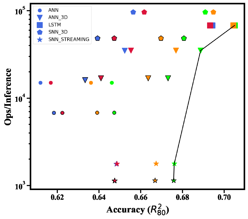
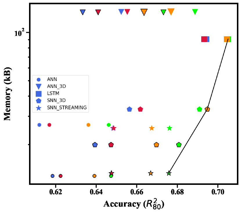
Figure 10: Pareto plots showing trade-offs for different models with increased training data to $80\%$ from the originally used $50\%$: a) Compute cost vs. accuracy b) Memory footprint vs. accuracy

TABLE III: Baseline Performance and Comparison with Prior Works

Models	Split	Filters	R2	Activation	Computes			Model Size $($ kB $)$
				Sparsity
					MACs	ACs	Memory access
ANN	50%	No Filter [17]	0.5818	0.7514	4969.76	0	5,179.46	26.5234
		Fwd Filtering	0.5874	0.7514	4971.76	0	5,181.46	26.5312
		Block Bid Filtering	0.6064	0.7514	4972.76	0	5,182.46	26.5351
		Bid Filtering	0.6168	0.7514	4974.76	0	5,184.46	26.5429
	80%	No Filter	0.6119 $($+0.03$)$	0.7417	5000.25	0	5,205.65	26.5234
		Fwd Filtering	0.6169 $($+0.03$)$	0.7417	5002.25	0	5,207.65	26.5312
		Block Bid Filtering	0.6361 $($+0.03$)$	0.7417	5003.25	0	5,208.65	26.5351
		Bid Filtering	0.6461 $($+0.03$)$	0.7417	5005.25	0	5,210.65	26.5429
ANN_3D	50%	No Filter [17]	0.6013	0.7348	11507.07	0	11,555.31	134.5234
		Fwd Filtering	0.6095	0.7348	11509.07	0	11,557.31	134.5312
		Block Bid Filtering	0.6495	0.7348	11510.07	0	11,558.31	134.5351
		Bid Filtering	0.656	0.7348	11512.07	0	11,560.31	134.5429
	80%	No Filter	0.6523 $($+0.05$)$	0.7324	11676.22	0	11,644.82	134.5234
		Fwd Filtering	0.6553 $($+0.05$)$	0.7324	11678.22	0	11,646.82	134.5312
		Block Bid Filtering	0.6769 $($+0.03$)$	0.7324	11679.22	0	11,647.82	134.5351
		Bid Filtering	0.6887 $($+0.03$)$	0.7324	11681.22	0	11,649.82	134.5429
SNN_3D	50%	No Filter [17]	0.6219	0	32256	0	39,057.79	33.1992
		Fwd Filtering	0.6318	0	32258	0	39,058.79	33.207
		Block Bid Filtering	0.6579	0	32259	0	39,059.79	33.2109
		Bid Filtering	0.6687	0	32261	0	39,062.79	33.2187
	80%	No Filter	0.6564 $($+0.03$)$	0	32256	0	39,701.38	33.1992
		Fwd Filtering	0.6617 $($+0.03$)$	0	32258	0	39,702.38	33.207
		Block Bid Filtering	0.6948 $($+0.04$)$	0	32259	0	39,703.38	33.2109
		Bid Filtering	0.6909 $($+0.02$)$	0	32261	0	39,706.38	33.2187
SNN_Streaming	50%	No Filter	0.6112	0.7453	0	971.26	1,195.28	25.32
		Fwd Filtering	0.6109	0.7453	0	973.26	1,197.28	25.3278
		Block Bid Filtering	0.6342	0.7453	0	974.26	1,198.28	25.3317
		Bid Filtering	0.6458	0.7453	0	976.26	1,200.28	25.3395
	80%	No Filter	0.6483 $($+0.04$)$	0.7795	0	883.36	1,044.23	25.32
		Fwd Filtering	0.6486 $($+0.04$)$	0.7795	0	885.36	1,046.23	25.3278
		Block Bid Filtering	0.6674 $($+0.03$)$	0.7795	0	886.36	1,047.23	25.3317
		Bid Filtering	0.6761 $($+0.03$)$	0.7795	0	888.36	1,049.23	25.3395
LSTM	50%	No Filter	0.6508	0	22687.97	0	22913.27	90.95
		Fwd Filtering	0.6506	0	22690.97	0	22915.27	90.96
		Block Bid Filtering	0.6669	0	22690.97	0	22916.27	90.96
		Bid Filtering	0.6683	0	22690.97	0	22918.27	90.96
	80%	No Filter	0.6943 $($+0.04$)$	0	22687.97	0	22912.40	90.95
		Fwd Filtering	0.6932 $($+0.04$)$	0	22690.97	0	22914.40	90.96
		Block Bid Filtering	0.7044 $($+0.04$)$	0	22690.97	0	22915.40	90.96
		Bid Filtering	0.7051 $($+0.04$)$	0	22690.97	0	22917.40	90.96
SNN 2D[17]	50%	-	0.5805	0.9976	0	413.52	-	28.56
rEFH_dynamic [15]	320s∗	-	0.6319 $($bin_width=128$)$	-	-	-	-	-

V Discussion

This section discusses additional control experiments and gives an outlook for future improvements.

V-A Effect of Reach Removal

As mentioned in Section III-F, some of the reaches in the dataset spanned a much longer duration (sometimes longer than 200 seconds) than the rest which mostly were less than 4 seconds. These reaches (longer than 8 seconds) were removed from training since the NHP was likely unattentive in these cases. However, they were not removed from the testing data and hence, we explored how much improvement in performance is obtained by better curating the test dataset. These results are presented in the Table IV and we can observe that the $R^{2}$ increases by $\approx 0.01$ with the baseline 50% split–the improvement can be much more if other files from [15] are selected. This underlines the effectiveness and necessity of careful data selection from the recordings in [15] while training and testing models.

TABLE IV: Effect of Reach Removal

Models	Split	Filters	R2
ANN	50%	No Filter	0.5921 $($+0.01$)$
		Fwd Filtering	0.5977 $($+0.01$)$
		Block Bid Filtering	0.6155 $($+0.009$)$
		Bid Filtering	0.6249 $($+0.008$)$
ANN_3D	50%	No Filter	0.6133 $($+0.01$)$
		Fwd Filtering	0.6225 $($+0.01$)$
		Block Bid Filtering	0.6588 $($+0.009$)$
		Bid Filtering	0.6690 $($+0.01$)$
SNN_3D	50%	No Filter	0.6286 $($+0.007$)$
		Fwd Filtering	0.6437 $($+0.01$)$
		Block Bid Filtering	0.6652 $($+0.007$)$
		Bid Filtering	0.6755 $($+0.007$)$
SNN_Streaming	50%	No Filter	0.6212 $($+0.01$)$
		Fwd Filtering	0.6208 $($+0.01$)$
		Block Bid Filtering	0.6433 $($+0.009$)$
		Bid Filtering	0.6542 $($+0.008$)$
LSTM	50%	No Filter	0.6784 $($+0.03$)$
		Fwd Filtering	0.6779 $($+0.03$)$
		Block Bid Filtering	0.6788 $($+0.01$)$
		Bid Filtering	0.6800 $($+0.01$)$

V-B Latency of Filters

Latency between input and output is important for real-time applications with closed-loop operation such as motor decoding. The total time, $T_{tot}$, taken to produce an output by a NN decoder is given by $T_{tot}=St+T_{comp}$ where $St$ is the stride to capture the new input data ($=T_{GT}=4$ ms in this work) and $T_{comp}$ is the time taken to process the computations in the neural network. Given the very fast and energy-efficient In-memory computing (IMC) approaches to implement NN models prevalent now[32, 33] and the small networks considered in this paper, we can assume $T_{comp}<<St$ making the throughput almost entirely dependent on $St$, i.e. time taken to capture new neural input spikes. Note that the bin window, $T_{W}$ does not add any extra penalty on latency of output generation; however, after every change of target, the prediction will be inaccurate for a time related to $T_{W}$ to allow enough relevant input to fill up the bin window. However, output filtering may induce an extra penalty on the latency. Bid filters produced best results as seen in the earlier section; however, they cannot be employed in real-time applications since they need to store the raw data in memory first and then apply forward filtering two times in opposite directions. The block Bid filter is chosen as a compromise where the filter window is used to determine the length or block of samples that are filtered at one time, and the predicted point is located at the center of the sample window. Thus, the latency introduced by the block Bid filter is theoretically equal to half the length of the filter window. In this paper, window size was fixed to 16 samples resulting in a latency of $32$ ms. While this is acceptable in motor decoding, other applications may require lower latency. One possibility is to use analog Bessel filters which do not require such Bid filtering and this will be a focus of future work.

V-C Future Directions

The main reason for low energy consumption in SNN is due to the benefits of sparse activations. However, our experiment shows the sparsity may harm accuracy. We proposed two types of SNN models in this paper–one is SNN_3D, which has no sparsity due to the layer normalization, and another one is SNN_streaming, which has a relatively higher sparsity. Interestingly, the low power characteristic of SNN is not reflected in the first SNN model, whereas it has relatively higher accuracy. This points to the need for future research into data normalization techniques which can still retain sparsity of activations. Another reason for the high accuracy of SNN_3D was its reset of membrane potential after every $T_{W}$. This implies the membrane potential during training and testing start at exactly the same value for any sequence of inputs making it easier for the network to recognize similar patterns of input. For SNN_streaming, since there is no regular reset mechanism, the membrane voltages during training and testing may be quite different which may hurt accuracy. Mitigating this issue with initial condition of streaming SNNs will be a part of future work.

We see different models along the pareto curve having different strengths. For example, models with block Bid filtering have high accuracy but high latency. Using multiple models to produce a combined output may be a useful strategy. For example, switching from a model with block Bid filter to one without a filter right after a change of target/context will help in balancing latency and accuracy.

Finally, all the weights used in this work used float 32 as the default precision. However, there is a significant amount of work to quantize the models for more efficient inference. Applying these approaches of quantization aware training should allow us to reduce the model footprint significantly in the future.

VI Conclusion

Scaling iBMI systems to tens of thousands of channels in the future as well as removing the connecting wires would require significant compression of data on the device to reduce wireless datarates. Integrating the signal processing chain up to the neural decoder offers interesting opportunities to maximize compression. In this context, this work explores the usage of different neural network models and combines them with traditional signal filtering techniques to explore accuracy vs cost trade-offs where the cost is measured in terms of memory footprint and number of operations. Adding Bessel filtering improves the performance of all five NN models with Bidirectional (Bid) and block Bid filtering generating the state-of-the-art results in offline and online filtering respectively. In general, LSTM and SNN_streaming models occupy the high and low ends of the pareto curves (for accuracy vs. memory/operations) respectively while SNN_3D and ANN_3D occupy intermediate positions.

Zhou Biyan received her Bachelors degree in Electrical Engineering from Hohai University and her Masters degree in Electrical and Electronic Engineering from Nanyang Technological University. She’s currently pursuing her PhD at the City University of Hong Kong, focusing on spiking neural network, neural decoder and brain machine interfaces.

Pao-Sheng Vincent Sun received his Bachelors in Computer Engineering and Masters in Electical and Electronic Engineering from the University of Western Australia. After graduation, he has worked in the automotive industry developing next generation smart lighting devices and setting up business analytics using machine learning with cloud computing. He is currently working towards his PhD at the City University of Hong Kong, with primary focus on computer vision based neuromorphic computing, spiking neural network and deep learning for edge application.

Arindam Basu Arindam Basu received the B.Tech and M.Tech degrees in Electronics and Electrical Communication Engineering from the Indian Institute of Technology, Kharagpur in 2005, the M.S. degree in Mathematics and PhD. degree in Electrical Engineering from the Georgia Institute of Technology, Atlanta in 2009 and 2010 respectively. Dr. Basu received the Prime Minister of India Gold Medal in 2005 from I.I.T Kharagpur. He is currently a Professor in City University of Hong Kong in the Department of Electrical Engineering and was a tenured Associate Professor at Nanyang Technological University before this. He is currently an Associate Editor of the IEEE Sensors journal, Frontiers in Neuroscience, IOP Neuromorphic Computing and Engineering, and IEEE Transactions on Biomedical Circuits and Systems. He has served as IEEE CAS Distinguished Lecturer for the 2016-17 period. Dr. Basu received the best student paper award at the Ultrasonics symposium, in 2006, the best live demonstration at ISCAS 2010, and a finalist position in the best student paper contest at ISCAS 2008. He was awarded MIT Technology Review’s TR35 Asia Pacific award in 2012 and inducted into Georgia Tech Alumni Association’s 40 under 40 class of 2022.

References

- [1] Zhang, M., Tang, Z., Liu, X. & Spiegel, J. Electronic neural interfaces. Nature Electronics. 3, 191-200 (2020)
- [2] Pandarinath, C. & Al. High performance communication by people with paralysis using an intracortical brain-computer interface. ELife. pp. e18554 (2017)
- [3] Libedinsky, C., So, R. & Al Independent mobility achieved through a wireless brain-machine interface. PLOS One. 11 (2016)
- [4] Ajiboye, W. & Al. Restoration of reaching and grasping move- ments through brain-controlled muscle stimulation in a person with tetraplegia: a proof-of-concept demonstration. The Lancet. 10081 pp. 1821-1830 (2017)
- [5] Metzger, S. & Et.al. A high-performance neuroprosthesis for speech decoding and avatar control. Nature. 620 pp. 1037-1046 (2023)
- [6] Willett, F. & Et.al. A high-performance speech neuroprosthesis. Nature. 620 pp. 1031-1036 (2023)
- [7] Willett, F., Avansino, D., Hochberg, L., Henderson, J. & Shenoy, K. High-performance brain-to-text communication via handwriting. Nature. 593, 249-254 (2021,5), https://doi.org/10.1038/s41586-021-03506-2
- [8] Basu, I., Yousefi, A., Crocker, B., Zelmann, R., Paulk, A., Peled, N., Ellard, K., Weisholtz, D., Cosgrove, G., Deckersbach, T., Eden, U., Eskandar, E., Dougherty, D., Cash, S. & Widge, A. Closed-loop enhancement and neural decoding of cognitive control in humans. Nature Biomedical Engineering. 7, 576-588 (2021,11), https://doi.org/10.1038/s41551-021-00804-y
- [9] Musk, E. An Integrated Brain-Machine Interface Platform With Thousands of Channels. Journal Of Medical Internet Research. 21, e16194 (2019,10), https://doi.org/10.2196/16194
- [10] Yin, B. & Al. An Implantable Wireless Neural Interface for Recording Cortical Circuit Dynamics in Moving Primates. Journal Of Neural Engineering. 10 (2013)
- [11] Stevenson, I. & Kording, K. How advances in neural recording affect data analysis. Nature Biomedical Engineerng. 14 pp. 139-142 (2011,1)
- [12] Chen, N. & Al. Power-saving design opportunities for wireless intracortical brain–computer interfaces. Nature Biomedical Engineering. 4 pp. 984-996 (2020)
- [13] Basu, A., Yi, C. & Enyi, Y. Big Data Management in Neural Implants: The Neuromorphic Approach. Emerging Technology And Architecture For Big-data Analytics. pp. 293-311 (2017)
- [14] Shaikh, S., So, R., Sibindi, T., Libedinsky, C. & Basu, A. Towards Intelligent Intracortical BMI (i²BMI): Low-Power Neuromorphic Decoders That Outperform Kalman Filters. IEEE Transactions On Biomedical Circuits And Systems. 13, 1615-1624 (2019)
- [15] Makin, J., O’Doherty, J., Cardoso, B., M. & Sabes, P. Superior arm-movement decoding from cortex with a new, unsupervised-learning algorithm. Journal Neural Engineering. 15 (2018)
- [16] Willsey, M., Nason-Tomaszewski, S., Ensel, S., Temmar, H., Mender, M., Costello, J., Patil, P. & Chestek, C. Real-time brain-machine interface in non-human primates achieves high-velocity prosthetic finger movements using a shallow feedforward neural network decoder. Nature Communications. 13, 6899 (2022)
- [17] Yik, J., Ahmed, S., Ahmed, Z., Anderson, B., Andreou, A., Bartolozzi, C., Basu, A., Blanken, D., Bogdan, P., Bohte, S. & Others NeuroBench: Advancing neuromorphic computing through collaborative, fair and representative benchmarking. ArXiv Preprint ArXiv:2304.04640. (2023)
- [18] Stevenson, I. Tracking advances in neural recording. Statistical Neuroscience Lab., https://stevenson.lab.uconn.edu/scaling/
- [19] Georgopoulos, A., Schwartz, A. & Kettner, R. Neuronal population coding of movement direction. Science. 233, 1416-1419 (1986)
- [20] Koyama, S., Chase, S., Whitford, A., Velliste, M., Schwartz, A. & Kass, R. Comparison of brain–computer interface decoding algorithms in open-loop and closed-loop control. Journal Of Computational Neuroscience. 29 pp. 73-87 (2010)
- [21] Kim, S., Simeral, J., Hochberg, L., Donoghue, J. & Black, M. Neural control of computer cursor velocity by decoding motor cortical spiking activity in humans with tetraplegia. Journal Of Neural Engineering. 5, 455 (2008)
- [22] Hochberg, L., Bacher, D., Jarosiewicz, B., Masse, N., Simeral, J., Vogel, J., Haddadin, S., Liu, J., Cash, S., Van Der Smagt, P. & Others Reach and grasp by people with tetraplegia using a neurally controlled robotic arm. Nature. 485, 372-375 (2012)
- [23] Sharma, G., Friedenberg, D., Annetta, N., Glenn, B., Bockbrader, M., Majstorovic, C., Domas, S., Mysiw, W., Rezai, A. & Bouton, C. Using an artificial neural bypass to restore cortical control of rhythmic movements in a human with quadriplegia. Scientific Reports. 6, 33807 (2016)
- [24] Friedenberg, D., Schwemmer, M., Landgraf, A., Annetta, N., Bockbrader, M., Bouton, C. & Others Neuroprosthetic-enabled control of graded arm muscle contraction in a paralyzed human. Sci Rep. 2017; 7: 8386.
- [25] Zhang, Z. & Constandinou, T. Firing-rate-modulated spike detection and neural decoding co-design. Journal Of Neural Engineering. 20, 036003 (2023,5), https://dx.doi.org/10.1088/1741-2552/accece
- [26] Moses, D., Metzger, S., Liu, J., Anumanchipalli, G., Makin, J., Sun, P., Chartier, J., Dougherty, M., Liu, P., Abrams, G., Tu-Chan, A., Ganguly, K. & Chang, E. Neuroprosthesis for Decoding Speech in a Paralyzed Person with Anarthria. New England Journal Of Medicine. 385, 217-227 (2021,7), https://doi.org/10.1056/nejmoa2027540
- [27] Schuman, C., Kulkarni, S., Parsa, M., Mitchell, J., Date, P. & Kay, B. Opportunities for neuromorphic computing algorithms and applications. Nature Computational Science. 2, 10-19 (2022,1)
- [28] Liao, J., Widmer, L., Wang, X., Di Mauro, A., Nason-Tomaszewski, S., Chestek, C., Benini, L. & Jang, T. An Energy-Efficient Spiking Neural Network for Finger Velocity Decoding for Implantable Brain-Machine Interface. 2022 IEEE 4th International Conference On Artificial Intelligence Circuits And Systems (AICAS). pp. 134-137 (2022)
- [29] O’Doherty, J., MB, M., Makin, J. & Sabes, P. Nonhuman primate reaching with multichannel sensorimotor cortex electrophysiology. (https://zenodo.org/records/583331)
- [30] Chen, Y., Yao, E. & Basu, A. A 128-Channel Extreme Learning Machine-Based Neural Decoder for Brain Machine Interfaces. IEEE Trans. On Biomedical Circuits And Systems. 10, 679-692 (2016)
- [31] Horowitz, M. 1.1 computing’s energy problem (and what we can do about it). 2014 IEEE International Solid-state Circuits Conference Digest Of Technical Papers (ISSCC). pp. 10-14 (2014)
- [32] Sebastian, A. & Al. Memory devices and applications for in-memory computing. Nature Nanotechnology. 15, 529-544 (2020)
- [33] Zhang, C. & Al. Challenges and trends of SRAM-based computing-in-memory for AI edge devices. IEEE Trans. On CAS-I. 68, 1773-1786 (2021)