PBCounter: Weighted Model Counting on Pseudo-Boolean Formulas

Abstract

In Weighted Model Counting (WMC), we assign weights to literals and compute the sum of the weights of the models of a given propositional formula where the weight of an assignment is the product of the weights of its literals. The current WMC solvers work on Conjunctive Normal Form (CNF) formulas. However, CNF is not a natural representation for human-being in many applications. Motivated by the stronger expressive power of pseudo-Boolean (PB) formulas than CNF, we propose to perform WMC on PB formulas. Based on a recent dynamic programming algorithm framework called ADDMC for WMC, we implement a weighted PB counting tool $\mathsf{PBCounter}$. We compare $\mathsf{PBCounter}$ with the state-of-the-art weighted model counters SharpSAT-TD, ExactMC, D4, and ADDMC, where the latter tools work on CNF with encoding methods that convert PB constraints into a CNF formula. The experiments on three domains of benchmarks show that $\mathsf{PBCounter}$ is superior to the model counters on CNF formulas.

Weighted Model Counting, Pseudo-Boolean Constraint, Algebraic Decision Diagrams, Preprocessing Techniques.

1 Introduction

Model counting is a fundamental problem in computer science with a wide variety of applications in practice, ranging from neural network verification [1], network reliability [2], computational biology [3], and the like. Given a propositional formula $\varphi$, the model counting problem is to compute the number of satisfying assignments of $\varphi$. Weighted Model Counting (WMC) is a generalization of model counting. In WMC, we assign weights to literals and compute the sum of the weights of the models of $\varphi$ where the weight of an assignment is the product of the weights of its literals. The WMC solvers can serve as efficient tools for probabilistic inference [4, 5, 6], and many applications benefit significantly from WMC-based probabilistic inference, including probabilistic planning [7], probabilistic databases [8], and probabilistic programming [9].

The major approaches to the design of scalable (exact) model counters are mainly divided into three types: (1) search-based, (2) compilation-based, and (3) variable elimination-based methods [10]. The search-based techniques predominately focus on the combination of component caching with Conflict Driven clause learning including Cachet [11], sharpSAT [12] and Ganank [13]. The compilation-based techniques rely on the paradigm of knowledge compilation. Target languages of interest include d-DNNF and CCDD, with two counters based on them, D4 and ExactMC [14, 10]. Recently variable elimination-based techniques have been proposed, ADDMC uses the early project to eliminate variables represented by Algebraic Decision Diagrams [15]. NestHDB is a scalable hybrid tool that combines search-based and variable elimination-based counting methods [16]. There are also many approximate model counters, such as STS [17], ApproxMC [18], and PartialKC [19].

The current WMC solvers work on Conjunctive Normal Form (CNF) formulas. However, CNF is not a natural representation of human-beings in many applications. A Pseudo-Boolean (PB) constraint is of the form $\sum_{i=1}^{n}a_{i}l_{i}\vartriangleright b$, where the $a_{i}$ and $b$ are integers, literal $l_{i}$ is a Boolean variable $x_{i}$ or its negation, and the relation operator $\vartriangleright\in\{<,\leq,=,\geq,>\}$. PB constraints are a natural generalization of clauses in CNF; e.g., a clause $l_{1}\lor l_{2}\lor\dots\lor l_{m}$ is equivalent to the PB constraint $\sum_{i=1}^{m}l_{i}\geq 1$. Compared with clauses, it is easier to use PB constraints to describe the arithmetic properties of a problem. Moreover, PB constraints are strictly more succinct than a CNF formula according to the criteria used in the knowledge compilation map [20]. Thus, PB constraints have been widely used to efficiently represent many problems ranging from wireless sensor network [21] and logic synthesis [22] to Minimum-Width Confidence Bands [23].

Currently, a general approach to solving the problems modeled in PB constraints is to encode them into a CNF formula with the same satisfiability or model count and then employ a SAT solver or model counter to solve the resulting CNF formula. The clear benefit of this approach is due to the high-performance of the modern SAT solvers and model counters. However, the encoding from a PB formula to CNF introduces many auxiliary variables, and thus increases the size of the problem and even sometimes damages the structure or semantics of the original constraints. For these reasons, developing tools that work directly on PB formulas makes sense.

For the satisfiability of PB constraints, there exist many complete tools that directly work on PB formulas, such as PBS [24], PUEBLO [25], and RoundingSat [26]. These tools are more efficient on PB constraints since they use cutting planes proof system to analyze conflicts, which was shown exponentially more powerful than the resolution-based proof system in normal SAT solving. There exist some incomplete tools for PB Optimization such as NuPBO [27] and DeepOpt-PBO [28] as well. Turning to model counting or WMC, there are no tools that directly work on PB formulas so far. In this study, we propose to perform WMC on PB formulas. Based on a recent dynamic programming algorithm framework called ADDMC for WMC on CNF formulas, we implement a weighted PB counting tool $\mathsf{PBCounter}$. Our experiments have demonstrated that $\mathsf{PBCounter}$ was able to solve the greatest number of instances and was the fastest on most of them.

Model counting on PB constraints can also be viewed as a counting problem for 0-1 integer linear programming, which is a simplified version of integer linear programming (ILP) that restricts the variables to take values of 0 or 1. Counting integer solutions of ILP has important applications such as simple temporal planning [29] and probabilistic program analysis [30]. In practice, however, it is often difficult to count the solutions of an ILP problem with a great dimension [31]. We compare $\mathsf{PBCounter}$ with the ILP counter IntCount[32], and the experimental results show that $\mathsf{PBCounter}$ has a significant advantage.

The rest of the paper is organized as follows: We present notations and preliminaries in Section 2. Our algorithm of $\mathsf{PBCounter}$ is presented in Section 3. In Section 4, we present two preprocessing techniques on PB Constraints. Next, we present a detailed empirical evaluation in Section 5. Finally, we conclude in Section 6.

2 Preliminaries

In this section, we introduce the background knowledge about Weighted Model Counting (WMC), Pseudo-Boolean (PB) constraints, and Algebraic Decision Diagram (ADD), the primary data structure we used in our tool $\mathsf{PBCounter}$.

2.1 Weighted Model Counting

Given a set of Boolean variables $\{x_{1},x_{2}\ldots x_{n}\}$, a literal is either a variable $x_{i}$ or its negation $\overline{x_{i}}$. The negation of a literal $l$, written $\overline{l}$, denotes $\overline{x}$ if $l$ is $x$, and $x$ if $l$ is $\overline{x}$. A clause is a disjunction of literals. A conjunctive normal form (CNF) formula $F=c_{1}\land c_{2}\land\dots\land c_{m}$ is a conjunction of clauses.

Definition 1 (Weighted Model Counting).

Given a CNF formula $\psi$ over variables set $X$, $\psi$ can be represented as a Boolean function $\psi:2^{X}\to\{0,1\}$. Let $W:2^{X}\to\mathbb{R}$ be an arbitrary function representing the weight of assignments. The weighted model count of $\psi$ w.r.t. $W$ is $W(\psi)=\sum_{\tau\in 2^{X}}\psi(\tau)\cdot W(\tau)$ .

The function $W:2^{X}\to\mathbb{R}$ is called the weight function. The weight of an assignment is the product of the weight of its literals. Next, we define two operations that are useful for WMC solving.

Definition 2 (Product).

Let $X$ and $Y$ be sets of variables. The product of functions $f:2^{X}\to\mathbb{R}$ and $g:2^{Y}\to\mathbb{R}$ is the function $f\cdot g:2^{X\cup Y}\to\mathbb{R}$ defined for all $\tau\in 2^{X\cup Y}$ by $(f\cdot g)(\tau):=f(\tau_{X})\cdot g(\tau_{Y})$ .

In Definition 2, $\tau_{X}$ is the projection of $\tau$ over variable set $X$. Operation $product$ is commutative and associative. If we use Boolean function $\varphi:2^{X}\to\{0,1\}$ and $\psi:2^{Y}\to\{0,1\}$ to represent two CNF formulas, the product $\varphi\cdot\psi$ is the Boolean function corresponding to the conjunction $\varphi\land\psi$.

Definition 3 (Projection).

Let $X$ be a set of variables and $x\in X$. The projection of $f:2^{X}\to\mathbb{R}$ w.r.t. $x$ is the function $\Sigma_{x}f:2^{X\setminus\{x\}}\to\mathbb{R}$ defined for all $\tau\in 2^{X\setminus\{x\}}$ by $(\Sigma_{x}f)(\tau):=f(\tau\cup\{x\})+f(\tau\cup\{\overline{x}\})$ .

Note that projection is commutative, i.e., that $\Sigma_{x}\Sigma_{y}f=\Sigma_{y}\Sigma_{x}f$ for all variables $x,y\in X$ and functions $f:2^{X}\to\mathbb{R}$. Given a set $X=\{x_{1},x_{2},\dots,x_{n}\}$, we define $\Sigma_{X}f=\Sigma_{x_{1}}\Sigma_{x_{2}}\dots\Sigma_{x_{n}}f$ and $\Sigma_{\varnothing}f=f$.

The equation in Definition 1 can be expressed in an alternative form as $W(\psi)=(\Sigma_{X}(\psi\cdot W))(\varnothing)$, whose computation relies on the operations of product and projection. Dudek et al. showed that a special type of projection, called early projection, can accelerate WMC solving [15].

Theorem 1 (Early projection).

Let $X$ and $Y$ be sets of variables. Given $f:2^{X}\to\mathbb{R}$ and $g:2^{Y}\to\mathbb{R}$, if $x\in X\setminus Y$, then $\Sigma_{x}(f\cdot g)=(\Sigma_{x}f)\cdot g$ .

The early projection has critical applications in many fields, such as database-query optimization [33], satisfiability solving [34]. and weighted model counting  [15].

2.2 Pseudo-Boolean Constraints

A Pseudo-Boolean (PB) constraint is of the form $\sum_{i=1}^{n}a_{i}l_{i}\vartriangleright b$, where the $a_{i}$ and $b$ are integers, literal $l_{i}$ is a Boolean variable $x_{i}$ or its negation $\overline{x_{i}}$, i.e., $\overline{l_{i}}=1-l_{i}$, and the relation operator $\vartriangleright\in\{<,\leq,=,\geq,>\}$. The right side of the constraint $b$ is often called the degree of the constraint. PB constraints are more expressive than clauses. Actually, each clause is a special PB constraint in which degree $b$ and all coefficients $a_{i}$ are $1$, and $\vartriangleright$ is $\geq$.

A PB formula $\varphi$ is a conjunction of PB constraints. $\varphi$ can be represented as a Boolean function $\varphi:2^{X}\to\{0,1\}$. A complete truth assignment is a mapping that assigns to each variable in the set $X$ either $0$ or $1$. In PB, a constraint is satisfied when the equality holds. Therefore we can regard the PB formulas as a mapping from truth assignment to satisfiability. We use $\gamma:2^{X_{\gamma}}\to\{0,1\}$ to represent a constraint $\gamma\in\varphi$, where $X_{\gamma}\subseteq X$ is the set of variables appearing in $\gamma$.

There are many efficient methods for encoding PB constraints into CNF so that we can directly use the tools on CNF to solve the reasoning problems on PB. Eén et al. describe and evaluate three different techniques, translating by BDDs, Adder Network, and Sorting Network [35]. There are many studies that have made transformations for a special type of PB constraints, e.g., at-most-one constraints and PBMod-constraints [36, 37].

2.3 Algebraic Decision Diagrams

Algebraic Decision Diagram (ADD) is a compact representation of a function as a directed acyclic graph [38]. It is an extension of the Binary Decision Diagram (BDD) that represents functions mapping each state to a finite set of values, e.g., integers representing costs.

We consider an ADD $\mathcal{A}$ over a set of Boolean variables $X$ and an arbitrary set $S$. $\mathcal{A}$ is a rooted directed acyclic graph where each node of $\mathcal{A}$ is an element in either $X$ or $S$. Every terminal node of $\mathcal{A}$ is labeled with an element of $S$, and every non-terminal node of $\mathcal{A}$ is labeled with an element of $X$ and has two out-going edges labeled $0$ and $1$ (0-edge and 1-edge for short). For the directed path from the root to the terminal node in $\mathcal{A}$, the element represented by the non-terminal node on the path will appear no more than once.

3 WMC on PB Constraints

In this section, we introduce the algorithmic framework for weighted model counting on PB constraints. We first define the WMC task on PB as follows:

Definition 4 (Model Counting on PB Constraints).

Let $\varphi$ be a PB formula over variables set $X$, and let $W:2^{X}\to\mathbb{R}$ be an arbitrary function. The weighted model count on $\varphi$ w.r.t. $W$ is defined as $W(\varphi)=\sum_{\tau\in 2^{X}}\varphi(\tau)\cdot W(\tau)$ .

Obviously, the product operation can be used to represent the entire formula by constraints, i.e., $\varphi=\prod_{\gamma\in\varphi}\gamma$. Then the equation in Definition 4 can be rewritten as $W(\varphi)=(\Sigma_{X}(\varphi\cdot W))(\varnothing)$. Just like ADDMC, our WMC algorithm uses ADDs to perform products and projections. To facilitate the transformation from PB constraints to ADDs, we normalize the PB constraints. It is widely recognized that the PB constraint can be normalized using only one operator, such as $\geq$. In this context, a constraint $\sum_{i=1}^{n}a_{i}l_{i}=b$ is split into two constraints $\sum_{i=1}^{n}a_{i}l_{i}\geq b$ and $\sum_{i=1}^{n}a_{i}(\overline{l_{i}}-1)\geq-b$. However, when computing WMC, we need to perform product between constraints, and therefore the split incurs an additional cost. To address this issue, we relax the standard normalized PB constraint to admit $=$ in addition to $\geq$.

Definition 5 (Relaxed normalized PB constraint).

Given a PB constraint $\sum_{i=1}^{n}a_{i}l_{i}\vartriangleright b$, it is relaxed normalized iff each coefficient $a_{i}$ is non-negative integer and operator $\vartriangleright$ is $\geq$ or $=$.

We can transform each PB constraint into a relaxed normalized PB constraint as follows. First, we transform $\vartriangleright$ into $\geq$ except for $=$. That is, we multiply both sides of the inequality by $-1$ to transform the operators $<$ (resp. $\leq$) into $>$ (resp. $\geq$), and then we can replace $>b$ by $\geq b+1$. Second, we can replace $-al$ by $a\overline{l}-a$ to ensure every coefficient is a non-negative integer. Finally, if a relaxed normalized PB constraint has a negative degree, it cannot be satisfied and therefore the weighted model count is zero. Hereafter, we assume each PB constraint is relaxed normalized unless otherwise stated.

3.1 Dynamic Programming Framework

The focus of dynamic programming is to decompose complex problems into small sub-problems to solve and combine the solutions to get the answer. We extend the algorithmic framework of ADDMC [15] to solve the WMC on PB. Our algorithm is presented in Algorithm 1, and we will discuss our preprocessing techniques in Section 4 (line 1).

The input $\prec$ is called diagram variable order and is used to build ordered ADDs to support tractable products and projections. It determines the order of variable occurrence along the path from the root to the terminal node in ADDs and greatly influences the size of the diagram.

Another input $\rho$ is injection $X\to\mathbb{Z}^{+}$, where $X=\texttt{Vars}(\varphi)$ represents all variables appearing in formula $\varphi$. $\rho$ is used to partition PB constraints into several disjoint parts $\{\Gamma_{i}\}_{i=1}^{m}$, called clusters. According to these clusters, we get the partition $\{X_{i}\}_{i=1}^{m}$ of the variable set $X$. Variables already placed in $X_{i}$ will not be placed in $X_{1},\dots X_{i-1}$. This property allows us to early project the variables in $X_{i}$ (line 11), because they will not appear later.

Input: nonempty PB formula $\varphi$, literal-weight function $W$ over $X=\texttt{Vars}(\varphi)$, diagram variable order $\prec$, cluster variable order $\rho$

Output: $W(\varphi)$ weighted PB count of $\varphi$ w.r.t. $W$

1

2$\varphi\leftarrow\texttt{preprocess}(\varphi)$

3 $m\leftarrow\max_{x\in Vars(\varphi)}\rho(x)$

4 $\varphi\leftarrow\texttt{sort}(\varphi,\prec)$

5for $i=m,m-1,\dots 1$ do

6       $\Gamma_{i}\leftarrow\{\gamma\in\varphi:\texttt{constraintRank}(\gamma,\rho)=i\}$

7       $\kappa_{i}\leftarrow\{\texttt{constructEqADD}(\gamma,1,b):\gamma\in\Gamma_{i},\vartriangleright\text{is}=\}\cup\{\texttt{constructGEqADD}(\gamma,1,b):\gamma\in\Gamma_{i},\vartriangleright\text{is}\geq\}$

8       $X_{i}\leftarrow\texttt{Vars}(\Gamma_{i})\setminus\bigcup_{j=i+1}^{m}\texttt{Vars}(\Gamma_{j})$

9      

10for $i=1,2,\dots m$ do

11       if $\kappa_{i}\neq\varnothing$ then

12             $\mathcal{A}_{i}\leftarrow\prod_{D\in\kappa_{i}}D$ ;

13             for $x\in X_{i}$ do $\mathcal{A}_{i}\leftarrow\Sigma_{x}(\mathcal{A}_{i}\cdot W_{x})$;

14             if $i<m$ then

15                   $j\leftarrow\texttt{chooseCluster}(\mathcal{A}_{i},i)$

16                   $\kappa_{j}\leftarrow\kappa_{j}\cup\{\mathcal{A}_{i}\}$

17                  

18            

19      

return $\mathcal{A}_{m}(\varnothing)$

Algorithm 1 $\mathsf{PBCounter}$$(\varphi,W,\prec,\rho)$ : WMC on PB Constraints

We use $\kappa_{i}$ for each cluster to represent the set of ADDs in the cluster $\Gamma_{i}$. We product ADDs in $\kappa_{i}$ (line 10), do project, and insert the result ADD $\mathcal{A}_{i}$ into another cluster (line 14).

Heuristics are essential parts of Algorithm 1. We implement all the heuristics used in ADDMC for PB constraints and choose MCS (maximum-cardinality search [39]) and LexP (lexicographic search for perfect orders [40]) as the diagram variable order ($\prec$) and cluster variable order ($\rho$), respectively, and BM-Tree (Bouquet’s Method with tree data structure [15]) as the cluster heuristic for the function constraintRank and chooseCluster. This combination performed best in the experiment by ADDMC.

3.2 Construct ADDs for PB Constraints

We show how $\mathsf{PBCounter}$ constructs ADDs to represent PB constraints (line 6 in Algorithm 1). We use two different construction methods, described in Algorithms 2–3, for the PB constraints with operators $=$ and $\geq$, respectively.

Input: A PB constraint $\gamma:\sum_{i=1}^{n}a_{i}l_{i}=b$, integers $1\leq j\leq n+1,k$

Output: $\mathcal{A}$: ADD represent sub-constraint $\gamma^{\prime}:\sum_{i=j}^{n}a_{i}l_{i}=k$

1

2if $k<0$ then return $TerminalNode(0)$ // UNSAT for all assignments;

3 if $j=n+1$ then

4       if $k=0$ then return $TerminalNode(1)$ // Find a SAT assignment;

5       else return $TerminalNode(0)$;

6      

7$\mathcal{A}\leftarrow\texttt{findEqADD}(\gamma,j,k)$

8 if $\mathcal{A}\neq\varnothing$ then return $\mathcal{A}$;

9 $\mathcal{A}_{f}\leftarrow\texttt{constructEqADD}(\gamma,j+1,k)$

// $\mathcal{A}_{f}$ represent $\sum_{i=j+1}^{n}a_{i}l_{i}=k\land\overline{l_{j}}$

10 $\mathcal{A}_{t}\leftarrow\texttt{constructEqADD}(\gamma,j+1,k-a_{j})$

// $\mathcal{A}_{t}$ represent $(\sum_{i=j+1}^{n}a_{i}l_{i}=k-a_{j})\land l_{j}$

11

12if $l_{j}$ is positive then $\mathcal{A}\leftarrow\texttt{Ite}(x_{j},\mathcal{A}_{t},\mathcal{A}_{f})$;

13 else $\mathcal{A}\leftarrow\texttt{Ite}(x_{j},\mathcal{A}_{f},\mathcal{A}_{t})$;

14 storeEqADD$(\gamma,j,k,\mathcal{A})$

return $\mathcal{A}$

Algorithm 2 constructEqADD($\gamma,j,k$) : Construct ADD for sub-constraint $\gamma^{\prime}:\sum_{i=j}^{n}a_{i}l_{i}=k$

In Algorithm 2, we provide a recursive function for constructing ADD for constraint $\sum_{i=1}^{n}a_{i}l_{i}=b$. It divides the current constraint into two sub-constraints (lines 7-8) and solves them recursively, then constructs the ADD of the current constraint (lines 9-10). Ite$(x_{j},\mathcal{A}_{t},\mathcal{A}_{f})$, known as If-Then-Else, is an operation of ADDs, which returns an ADD rooted at $x_{j}$, 1-edge linked $\mathcal{A}_{t}$ and 0-edge linked $\mathcal{A}_{f}$. We use storeEqADD to store constructed sub-constraints with the same parameter $k$ (line 11), avoiding duplicate constructions. If the same ADD has been constructed before, we can return it directly (lines 5-6).

For each PB constraint with positive literals and $\leq$, Abío et al. proposed a linear algorithm for converting it into a reduced ordered BDD [41]. We modify this algorithm to make it be able to deal with negative literals and output ADDs, which is an extension of BDDs. For a PB constraint $\sum_{i=1}^{n}a_{i}l_{i}\geq b$, we can partition the interval $(-\infty,\infty)$ into multiple sub-intervals such that when $b$ belongs to the same sub-interval, their corresponding ADDs are the same. We use Example 1 to explain this point further.

Example 1.

The constraint $2x_{1}+3x_{2}\geq b$ with the order $x_{1}\prec x_{2}$ can correspond to five possible ADDs when $b$ has different values from five intervals, as shown in Figure 1. If $b\in(-\infty,0]$, every possible assignment over $\{x_{1},x_{2}\}$ satisfies the constraint, and we obtain a single ADD with only one terminal node labeled with $1$. Similarly, $2x_{1}+3x_{2}\geq 4$ and $2x_{1}+3x_{2}\geq 5$ will be both satisfied when $x_{1}=x_{2}=true$.

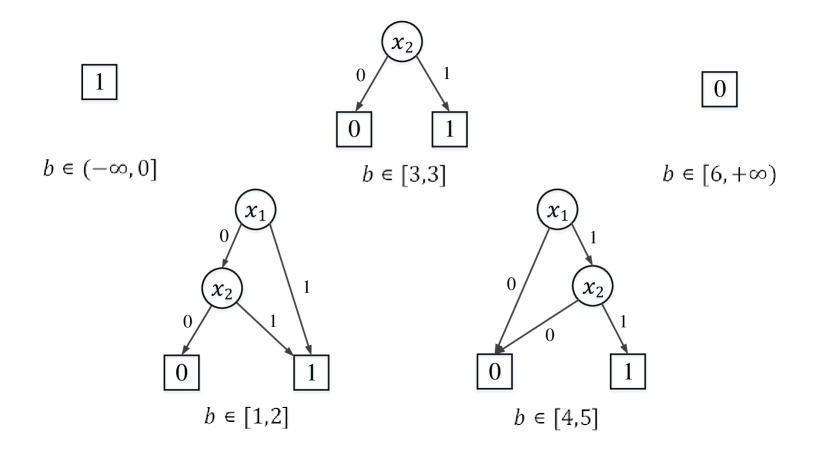
Figure 1: The five possible ADDs of $2x_{1}+3x_{2}\geq b$ over $x_{1}\prec x_{2}$.

The modified algorithm is presented in Algorithm 3. Consider a PB constraint $\sum_{i=1}^{n}a_{i}l_{i}\geq b$ with an order $x_{1}\prec x_{2}\prec\dots\prec x_{n}$. When we construct an ADD $\mathcal{A}$ for sub-constraint $\sum_{i=j}^{n}a_{i}l_{i}\geq k$, we store this ADD and the corresponding interval $[\alpha,\beta]$. When we compute a new sub-constraint $\sum_{i=j}^{n}a_{i}l_{i}\geq k^{\prime}$ with $k^{\prime}\in[\alpha,\beta]$, we can return the stored ADD and interval (lines 3–4). Otherwise, we need to recursively construct ADDs for sub-constraints (lines 5–6). With the outputs of recursive calls, we can compute the resulting ADD and the corresponding interval (lines 7–9).

Input: A PB constraint $\gamma:\sum_{i=1}^{n}a_{i}l_{i}\geq b$, integers $1\leq j\leq n+1,k$

Output: $[\alpha,\beta]$: interval contains $k$,
$\mathcal{A}$: ADD represent sub-constraint $\gamma^{\prime}:\sum_{i=j}^{n}a_{i}l_{i}\geq[\alpha,\beta]$

1

2if $k<0$ then

3      return $([-\infty,-1],TerminalNode(0))$

4if $k\geq\sum_{i=j}^{n}a_{i}$ then

5      return $([\sum_{i=j}^{n}a_{i},\infty],TerminalNode(1))$

6

7$([\alpha,\beta],\mathcal{A})\leftarrow\texttt{findGeqADD}(\gamma,j,k)$

// Find a stored ADD for $\gamma^{\prime}$ where $k\in[\alpha,\beta]$

8 if $\mathcal{A}\neq\varnothing$ then  return $([\alpha,\beta],\mathcal{A}$);

9

10$([\alpha_{f},\beta_{f}],\mathcal{A}_{f})\leftarrow\texttt{constructGEqADD}(\gamma,j+1,k)$

11 $([\alpha_{t},\beta_{t}],\mathcal{A}_{t})\leftarrow\texttt{constructGEqADD}(\gamma,j+1,k-a_{i})$

12 if $l_{j}$ is positive then $\mathcal{A}\leftarrow\texttt{Ite}(x_{j},\mathcal{A}_{t},\mathcal{A}_{f})$;

13 else $\mathcal{A}\leftarrow\texttt{Ite}(x_{j},\mathcal{A}_{f},\mathcal{A}_{t})$;

14 $[\alpha,\beta]\leftarrow[\alpha_{f},\beta_{f}]\cap[\alpha_{t}+a_{j},\beta_{t}+a_{j}]$

15

16$\texttt{storeGeqADD}(\gamma,j,[\alpha,\beta],\mathcal{A})$

return $([\alpha,\beta],\mathcal{A})$

Algorithm 3 constructGEqADD($\gamma,j,k$) : Construct ADD for sub-constraint $\gamma^{\prime}:\sum_{i=j}^{n}a_{i}l_{i}\geq k$

Note that Algorithm 3 returns a tuple of an interval $[\alpha,\beta]$ and ADD $\mathcal{A}$. That means every $k\in[\alpha,\beta]$ has same ADD $\mathcal{A}$ for sub-constraint $\gamma^{\prime}:\sum_{i=j}^{n}a_{i}l_{i}\geq k$. In line 5 of Algorithm 1, we need to ignore intervals and only keep ADDs in $\kappa_{i}$.

4 Preprocessing Techniques for WMC on PB

Efficient preprocessing techniques are an essential part of model counting solvers. Solvers like SharpSAT-TD and ExactMC have built-in preprocessors [42, 10], and some preprocessors designed explicitly for Model Counting, such as pmc and B+E [43], have also demonstrated the significance of preprocessing. However, there are no dedicated pre-processing techniques for WMC on PB currently. We first applied two preprocessing techniques to pseudo-Boolean formulas as our built-in preprocessing methods.

The first technique is based on the backbone. The backbone of a formula $\varphi$ is the set of all literals which are implied by $\varphi$ when $\varphi$ is satisfiable (variables that have the same value in all solutions) and is the empty set otherwise [44]. Algorithm 4 simplifies the PB formula $\varphi$ by identifying backbone variables and propagating unit literals on these backbone variables. In our implementation, we use RoundingSAT [26] to solve a PB formula and return a solution that satisfies the formula (lines 2, 4). If the formula is unsatisfiable, an empty set is returned. Similar to CNF, when a literal is determined to be true, the unit propagation on PB removes the literal and its negation from all other constraints. It simultaneously eliminates the term ($al$ or $a\overline{l}$) from both sides of the inequality. While the constraint is determined to be satisfiable, it can be deleted; if it is determined to be unsatisfiable, return $\bot$.

Input: A PB formula $\varphi$

Output: A PB formula equivalent to $\varphi$

1

2$\mathcal{B}\leftarrow\varnothing$

3 $\mathcal{I}\leftarrow\texttt{solve}(\varphi)$

4while $\exists l\in\mathcal{I}$ s.t. $l\notin\mathcal{B}$ do

5       $\mathcal{I}^{\prime}\leftarrow\texttt{solve}(\varphi\land\overline{l}\,)$

6       if $\mathcal{I}^{\prime}$ is $\varnothing$ then

7             $\mathcal{B}\leftarrow\mathcal{B}\cup\{l\}$

8             $\varphi\leftarrow\texttt{unitPropagate}(\varphi,l\,)\land\{l=1\}$

9      else $\mathcal{I}\leftarrow\mathcal{I}\cap\mathcal{I}^{\prime}$;

10      

11

return $\varphi$

Algorithm 4 addBackbone($\varphi$)

Since $\mathsf{PBCounter}$ requires the construction and operations of ADDs for each constraint, we propose the second preprocessing technique named deleteConstraint. It simplifies the formula by removing constraints $\gamma:[\varphi\setminus\gamma]\models\gamma$ representing in Algorithm 5. To verify $[\varphi\setminus\gamma]\models\gamma$, which is equivalent to $[\varphi\setminus\gamma]\land\overline{\gamma}\models\bot$, we transform $\gamma$ into its corresponding CNF formula, denoted as $c_{1}\land c_{2}\land\dots\land c_{m}$. Then, we can proceed to validate $[\varphi\setminus\gamma]\land(\overline{c_{1}}\lor\overline{c_{2}}\lor\cdots\lor\overline{c_{m}})\models\bot$. Using the algorithm presented in Section 3, we can construct a ADD $\mathcal{A}$ for constraint $\gamma$ (line 4). Each non-terminal node in $\mathcal{A}$ is labeled with a variable from $X$, and edges from each node represent literals (1-edge corresponds to positive literal, 0-edge corresponds to negative literal). That means all $\overline{c_{1}},\overline{c_{2}},\dots,\overline{c_{m}}$ are unsatisfiable assignments for $\gamma$, and correspond to the path from the root node to a terminal node labeled with 0 in $\mathcal{A}$ (line 5).

Example 2.

The PB formula $\varphi$ includes three constraints, $\gamma_{1}:3x_{1}+4x_{2}\geq 4$, $\gamma_{2}:3x_{1}+x_{3}+x_{4}\geq 4$, and $\gamma_{3}:3x_{2}+x_{3}+x_{4}\geq 4$. According to Figure 1, the ADD of $\gamma_{1}$ has two paths, $\overline{x_{1}}$ and $x_{1}\land\overline{x_{2}}$, to terminal node 0. Therefore, we get $\overline{c_{1}}=\overline{x_{1}}$ and $\overline{c_{2}}=x_{1}\land\overline{x_{2}}$. Since $[\gamma_{2}\land\gamma_{3}]\land\overline{c_{1}}\models\bot$ and $[\gamma_{2}\land\gamma_{3}]\land\overline{c_{2}}\models\bot$, we can delete $\gamma_{1}$ from $\varphi$.

To avoid the exponential explosion of ADD size, we do not attempt to delete constraints that involve more than 20 literals (line 2). We use unitPropagation to propagate all literals in unsatisfiable assignment $\overline{c_{i}}$ (line 8). If every $c_{i}$ satisfies $[\varphi\setminus\gamma]\land\overline{c_{i}}\models\bot$, $\gamma$ is removed.

Input: A PB formula $\varphi$

Output: A PB formula equivalent to $\varphi$

1

2foreach  $\gamma\in\varphi$  do

3       if $\texttt{notConsider}(\gamma)$ then continue;

4       $\varphi\leftarrow\varphi\setminus\{\gamma\}$

5       $\mathcal{A}=\texttt{constructADD}(\gamma)$

6       foreach path from root to $TerminalNode(0)$ in $\mathcal{A}$ do

7             $\varphi^{\prime}\leftarrow\varphi$

8             foreach literal l on path do

9                   $\varphi^{\prime}\leftarrow\texttt{unitPropagate}(\varphi^{\prime},l\,)$

10            if $\varphi^{\prime}$ is not $\bot$ then

11                   $\varphi\leftarrow\varphi\cup\{\gamma\}$

12                   break

13                  

14            

15      

16

return $\varphi$

Algorithm 5 deleteConstraint($\varphi$)

To achieve a more efficient implementation of Algorithm 5, we traverse all paths in $\mathcal{A}$ from the root to terminal nodes using a depth-first search. Based on the edges traversed along the path, we perform unit propagation on the literals it represented. When we reach the terminal node labeled 0 without encountering any conflicts, it implies there exists a $\overline{c_{i}}$ such that $[\varphi\setminus\gamma]\land\overline{c_{i}}\not\models\bot$. Therefore, the corresponding clause $\gamma$ can not be removed (line 10). We can directly backtrack when a conflict occurs on non-terminal nodes.

5 Experimental Results

In this section, we conducted experiments to evaluate the performance of our solver $\mathsf{PBCounter}$. We implemented $\mathsf{PBCounter}$ in C++. All experiments were run on a computer with Intel(R) Xeon(R) W-2133 CPU @ 3.60GHz and 64GB RAM.

5.1 Experiment Settings

As $\mathsf{PBCounter}$ is the first lazy WMC solver on PB constraints, we compare it with eager WMC solvers, an ILP counter, and a PB enumerator. We implemented two WMC encoding methods in C++ and combined them with four WMC counters on CNF. In other words, we have eight competitors for solving the WMC problem based on CNF, and two other approaches based on PB constraints. We ran each combination and $\mathsf{PBCounter}$ on each benchmark using a single core, 16 GB of memory, and 1800 seconds of the time limit.

Competitive Solvers

The four WMC solvers on CNF formulas include SharpSAT-TD, ExactMC, D4, and ADDMC. SharpSAT-TD is the winner of the Model Counting Competition 2021 - 2023 in the weighted track. It is based on solver SharpSAT and combines the technology of tree decomposition [12, 42]. ExactMC is based on CCDD (a generalization of Decision-DNNF), which can capture literal equivalences [10]. After compiling the instance into CCDD, ExactMC can compute model counts in linear time. D4 is a Decision-DNNF compiler that can calculate model counts by knowledge compilation [14]. ADDMC is the winner of the Model Counting Competition 2020 in the weighted track. It is a dynamic programming algorithm using ADD as the main data structure [15]. We use the decision diagram package Sylvan to manage ADDs in ADDMC and our solver $\mathsf{PBCounter}$. Sylvan can interface with the GNU Multiple Precision library to support ADDs with higher-precision numbers [45].

The two encoding methods we used are Warners [46] and ArcCons [47], which are proved counting safe [48]. We implemented the weighted encoders based on these two methods by keeping the original literals’ weights and setting the auxiliary literals’ weights to 1. This ensures that the weighted model counts are equal.

We also compared two other approaches. One is to run the PB solver RoundingSAT [26] to enumerate PB solutions and compute weighted model counts. The enumeration is achieved by continually adding the negation of the resulting satisfying assignments (called blocking clauses) to the formula to enumerate until the given formula is falsified. The other one uses ILP counter IntCount [32], which introduces column and row elimination techniques to decompose integer counting problems for linear constraints into independent sub-problems. Since IntCount cannot solve weighted instances, IntCount runs on an unweighted version of the benchmark.

Benchmarks

Our benchmarks consist of three parts. 1) We select instances from PB Competition 06, excluding clause-style instances since they can be solved directly with the WMC solver, resulting in 287 instances. 2) We select the benchmarks of Exact Cover used by Junttila and Kaski, consisting of 539 instances from 7 different problem families [49]. 3) According to the generator proposed by Kovásznai, we randomly generated 600 instances of Wireless Sensor Network (WSN) problem for six different combinations of three types of sensor and target nodes (5-2, 6-2, 7-3), and two constraint sets (all constraints on and evasive & moving off) [21]. One hundred instances were generated for each configuration.

For these instances, we randomly assigned weights $W(x)\in(0,1)$ and $1-W(x)$ to each $x$ and $\overline{x}$, respectively. For SharpSAT-TD, ExactMC, and D4, random weights have no effect on their performance. For ADDMC and $\mathsf{PBCounter}$, random weights may increase the number of terminal nodes in ADDs and therefore may increase the times of operating ADDs.

5.2 Evaluation

Experiment on Preprocessing Techniques

Firstly, we compared the impact of the preprocessing techniques mentioned in Section 4 on $\mathsf{PBCounter}$. We used "NoPre" to represent $\mathsf{PBCounter}$ without any preprocessing techniques, and "OnlyBb" to represent $\mathsf{PBCounter}$ with only the backbone technique (algorithm 4). Table 1 presents the results of the experiment for various benchmarks. We emphasize that the number of solved benchmarks only counts satisfiable instances. Unsatisfiable instances can be judged by pre-calling the PB or SAT solver and have no significance for model counting

Table 1: Results of Different Preprocessing Techniques

Benchmark (#)	NoPre	OnlyBb	$\mathsf{PBCounter}$
PB06 (287)	28	37	39
ExactCover (539)	192	193	194
WSN (600)	387	425	483
Total (1426)	607	655	716

The results show that the preprocessing techniques of algorithms 4 and 5 exhibit positive impacts across three different benchmarks. After incorporating preprocessing techniques into $\mathsf{PBCounter}$, the algorithm was able to solve an additional 109 instances in total. Additionally, using only backbone technique allows $\mathsf{PBCounter}$ to solve an additional 48 instances. Notably, the most significant enhancement was observed in the WSN benchmark.

Comparing with WMC Solvers on CNF

The performances of $\mathsf{PBCounter}$ and other counting combinations are summarized in Table 2 and Figure 2. $\mathsf{PBCounter}$ is the fastest solver in 327 instances and can uniquely solve 110 instances. $\mathsf{PBCounter}$_NoPre turns off preprocessing techniques and solves more instances than CNF-based WMC solvers; it uses the shortest time in 62 instances and uniquely solves 19 instances.

Two virtual best solvers: VBS1 shows the shortest solving time among all counters for each benchmark, while VBS0 shows the shortest time among eight WMC combinations (excluding $\mathsf{PBCounter}$). Except for $\mathsf{PBCounter}$, SharpSAT-TD solves the most number of instances, while ExactMC has shorter solving times on more instances.

Table 2: The number of instances solved by solvers.

Solvers	Instances Solved
	Unique	Fastest	Total
VBS1 (with $\mathsf{PBCounter}$)	-	-	750
VBS0 (without $\mathsf{PBCounter}$)	-	-	557
$\mathsf{PBCounter}$	110	327	716
$\mathsf{PBCounter}$_Nopre	19	62	607
SharpSAT-TD + Warner	3	11	531
SharpSAT-TD + ArcCons	0	2	520
ExactMC + Warner	0	3	511
ExactMC + GenArc	0	327	499
D4 + Warner	0	0	445
D4 + ArcCons	1	18	480
ADDMC + Warner	0	0	155
ADDMC + ArcCons	0	0	266

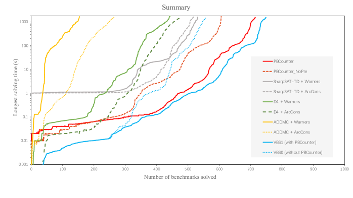
Figure 2: A cactus plot of the numbers of benchmarks solved by seven weighted model counters and two virtual best solvers (VBS1, with $\mathsf{PBCounter}$, and VBS0, without $\mathsf{PBCounter}$).

For the instances $\mathsf{PBCounter}$ uniquely solved, we observed that they often have long constraints. Encoding long constraints into CNF introduces more auxiliary variables and increases the difficulty of solving. Additionally, if only a few variables appear in multiple long constraints, $\mathsf{PBCounter}$ can reduce the size of ADDs by early projection before product computations.

Comparing with Different Approaches

We use "RSBlocking" to denote our implementation of the enumeration solver based on RoundingSAT [26]. IntCount is an ILP counter developed by Ge et al [32] based on Barvinok [50]. Table 3 shows the number of benchmarks solved by $\mathsf{PBCounter}$, RSBlocking, and IntCount.

Table 3: Results of Different Approaches

Benchmark (#)	$\mathsf{PBCounter}$	RSBlocking	IntCount
PB06 (287)	39	16	5
ExactCover (539)	194	178	8
WSN (600)	483	0	23
Total (1426)	716	194	36

RSBlocking performs well when the number of solutions is small, especially in the ExactCover benchmark. In fact, with only one solution, the enumeration algorithm only needs to call the PB solver twice. In the WSN benchmark, the time and space consumption of RSBlocking enumerated solutions becomes unsolvable due to the large satisfiable solution space. The ILP solver IntCount performs poorly in the three PB benchmarks, even if they are unweighted. We find that IntCount is more difficult to solve when the number of variables in instances is large and cannot be decomposed.

6 Conclusion and Future Work

In this work, we implemented the first lazy weighted model counter $\mathsf{PBCounter}$ on PB constraints with two preprocessing techniques. Like ADDMC, $\mathsf{PBCounter}$ is based on variable elimination and uses dynamic programming techniques. Our experiments show that $\mathsf{PBCounter}$ performed better than the eager state-of-the-art WMC tools; that is, encoding PB constraints into CNF formulas, and then employing ADDMC, SharpSAT-TD, ExactMC, or D4.

The studies [44, 51, 52] in model counting on CNF formulas show that the usage of pre-processing is critical for the performance of model counters. Our experimental results show that the proposed two preprocessing techniques are very effective in improving the performance of PBCounter, which is consistent with the previous studies. However, on the one hand, the implementation of the two pre-processing techniques is still relatively basic and can be improved further; on the other hand, we can still design more preprocessing techniques. For example, there is a lot of exciting work that can transform PB constraints and CNF formulas into each other with the counting-safe property. Therefore, we can first transform PB constraints into a CNF formula, then pre-process the CNF formula, and finally transform the pre-processed CNF formula into PB constraints. One future direction of this study is to develop a more effective pre-processor for the WMC task on PB constraints.

This work is supported by NSFC (under Grant No. 61976050, 61972384), Ministry of Education (under Grant No. 2021BCF01002), Jilin Province Natural Science Foundation, and Jilin Provincial Department of Education. Thanks to the editorial board and reviewers for their valuable comments.

pic/laiy.pngYong Lai is an Associate Professor at the College of Computer Science and Technology, Jilin University, China. He received his Ph.D. degree from Jilin University. His research interests include knowledge representation and reasoning, neural-symbolic computation, tractable machine learning, and probabilistic graphical model.

pic/xuzh.png Zhenghang Xu received a B.S. degree from Computer Science and Information Technology, Northeast Normal University, China in 2020. Currently, he is pursuing a Master’s degree at the College of Computer Science and Technology, Jilin University, China. His research interests include model counting and algorithm design.

pic/yinmh.pngMinghao Yin is a Professor at the School of Computer Science and Information Technology, Northeast Normal University, China. He received his Ph.D. degree in Computer Software and Theory from Jilin University, China. His research interests include heuristic search, data mining, and combinatorial optimization.

References

- [1] Teodora Baluta, Shiqi Shen, Shweta Shinde, Kuldeep S. Meel, and Prateek Saxena. Quantitative verification of neural networks and its security applications. In Proceedings of the 2019 ACM SIGSAC Conference on Computer and Communications Security, CCS 2019, pages 1249–1264, 2019.
- [2] Leonardo Dueñas-Osorio, Kuldeep S. Meel, Roger Paredes, and Moshe Y. Vardi. Counting-based reliability estimation for power-transmission grids. In Proc. of AAAI, 2 2017.
- [3] Palash Sashittal and Mohammed El-Kebir. SharpTNI: Counting and sampling parsimonious transmission networks under a weak bottleneck. In Proc. of RECOMB Comparative Genomics, 2019.
- [4] Dan Roth. On the hardness of approximate reasoning. Artificial Intelligence, 82:273–302, 1996.
- [5] Tian Sang, Paul Beame, and Henry A. Kautz. Performing bayesian inference by weighted model counting. In Manuela M. Veloso and Subbarao Kambhampati, editors, Proceedings, The Twentieth National Conference on Artificial Intelligence, pages 475–482. AAAI Press / The MIT Press, 2005.
- [6] Mark Chavira and Adnan Darwiche. On probabilistic inference by weighted model counting. Artificial Intelligence, 172(6–7):772–799, 2008.
- [7] Carmel Domshlak and Jörg Hoffmann. Probabilistic planning via heuristic forward search and weighted model counting. J. Artif. Intell. Res., 30:565–620, 2007.
- [8] Guy Van den Broeck and Dan Suciu. Query processing on probabilistic data: A survey. Foundations and Trends in Databases, 7(3-4):197–341, 2017.
- [9] Daan Fierens, Guy Van den Broeck, Joris Renkens, Dimitar Sht. Shterionov, Bernd Gutmann, Ingo Thon, Gerda Janssens, and Luc De Raedt. Inference and learning in probabilistic logic programs using weighted boolean formulas. TPLP, 15(3):358–401, 2015.
- [10] Yong Lai, Kuldeep S. Meel, and Roland H. C. Yap. The power of literal equivalence in model counting. In Thirty-Fifth AAAI Conference on Artificial Intelligence, AAAI 2021, pages 3851–3859. AAAI Press, 2021.
- [11] Tian Sang, Fahiem Bacchus, Paul Beame, Henry A. Kautz, and Toniann Pitassi. Combining component caching and clause learning for effective model counting. In SAT 2004 - The Seventh International Conference on Theory and Applications of Satisfiability Testing, 2004.
- [12] Marc Thurley. sharpsat - counting models with advanced component caching and implicit BCP. In Armin Biere and Carla P. Gomes, editors, Theory and Applications of Satisfiability Testing - SAT 2006, 9th, volume 4121 of Lecture Notes in Computer Science, pages 424–429. Springer, 2006.
- [13] Shubham Sharma, Subhajit Roy, Mate Soos, and Kuldeep S. Meel. GANAK: A scalable probabilistic exact model counter. In Sarit Kraus, editor, Proceedings of the Twenty-Eighth International Joint Conference on Artificial Intelligence, IJCAI 2019, pages 1169–1176. ijcai.org, 2019.
- [14] Jean-Marie Lagniez and Pierre Marquis. An improved decision-dnnf compiler. In Carles Sierra, editor, Proceedings of the Twenty-Sixth International Joint Conference on Artificial Intelligence, IJCAI 2017, pages 667–673. ijcai.org, 2017.
- [15] Jeffrey Dudek, Vu Phan, and Moshe Vardi. Addmc: weighted model counting with algebraic decision diagrams. In Proceedings of the AAAI Conference on Artificial Intelligence, volume 34, pages 1468–1476, 2020.
- [16] Markus Hecher, Patrick Thier, and Stefan Woltran. Taming high treewidth with abstraction, nested dynamic programming, and database technology. In Theory and Applications of Satisfiability Testing–SAT 2020: 23rd International Conference, Alghero, Italy, July 3–10, 2020, Proceedings 23, pages 343–360. Springer, 2020.
- [17] Stefano Ermon, Carla Gomes, and Bart Selman. Uniform solution sampling using a constraint solver as an oracle. In Proceedings of the Twenty-Eighth Conference on Uncertainty in Artificial Intelligence, pages 255–264, 2012.
- [18] Supratik Chakraborty, Kuldeep S Meel, and Moshe Y Vardi. A scalable approximate model counter. In Principles and Practice of Constraint Programming: 19th International Conference, CP 2013, pages 200–216. Springer, 2013.
- [19] Yong Lai, Kuldeep S Meel, and Roland HC Yap. Fast converging anytime model counting. In Proceedings of the AAAI Conference on Artificial Intelligence, volume 37, pages 4025–4034, 2023.
- [20] Daniel Le Berre, Pierre Marquis, Stefan Mengel, and Romain Wallon. Pseudo-boolean constraints from a knowledge representation perspective. In Jérôme Lang, editor, Proceedings of the Twenty-Seventh International Joint Conference on Artificial Intelligence, IJCAI 2018, pages 1891–1897, 2018.
- [21] Gergely Kovásznai, Balázs Erdélyi, and Csaba Biró. Investigations of graph properties in terms of wireless sensor network optimization. In 2018 IEEE International Conference on Future IoT Technologies (Future IoT), pages 1–8. IEEE, 2018.
- [22] Fadi A. Aloul, Arathi Ramani, Igor L. Markov, and Karem A. Sakallah. Generic ILP versus specialized 0-1 ILP: an update. In Lawrence T. Pileggi and Andreas Kuehlmann, editors, Proceedings of the 2002 IEEE/ACM International Conference on Computer-aided Design, ICCAD 2002, pages 450–457. ACM / IEEE Computer Society, 2002.
- [23] Zhendong Lei, Shaowei Cai, Chuan Luo, and Holger H. Hoos. Efficient local search for pseudo boolean optimization. In Chu-Min Li and Felip Manyà, editors, Theory and Applications of Satisfiability Testing - SAT 2021 - 24th, volume 12831 of Lecture Notes in Computer Science, pages 332–348. Springer, 2021.
- [24] Fadi A Aloul, Arathi Ramani, Igor Markov, and Karem Sakallah. Pbs: a backtrack-search pseudo-boolean solver and optimizer. In Proceedings of the 5th International Symposium on Theory and Applications of Satisfiability, pages 346–353, 2002.
- [25] Hossein M. Sheini and Karem A. Sakallah. Pueblo: A hybrid pseudo-boolean SAT solver. J. Satisf. Boolean Model. Comput., 2(1-4):165–189, 2006.
- [26] Jan Elffers and Jakob Nordström. Divide and conquer: Towards faster pseudo-boolean solving. In Proceedings of the Twenty-Seventh International Joint Conference on Artificial Intelligence, IJCAI 2018, pages 1291–1299, 2018.
- [27] Yi Chu, Shaowei Cai, Chuan Luo, Zhendong Lei, and Cong Peng. Towards more efficient local search for pseudo-boolean optimization. In 29th International Conference on Principles and Practice of Constraint Programming (CP 2023). Schloss Dagstuhl-Leibniz-Zentrum für Informatik, 2023.
- [28] Wenbo Zhou, Yujiao Zhao, Yiyuan Wang, Shaowei Cai, Shimao Wang, Xinyu Wang, and Minghao Yin. Improving local search for pseudo boolean optimization by fragile scoring function and deep optimization. In 29th International Conference on Principles and Practice of Constraint Programming (CP 2023). Schloss Dagstuhl-Leibniz-Zentrum für Informatik, 2023.
- [29] Amy Huang, Liam Lloyd, Mohamed Omar, and James Boerkoel. New perspectives on flexibility in simple temporal planning. In Proceedings of the International Conference on Automated Planning and Scheduling, volume 28, pages 123–131, 2018.
- [30] Kasper Luckow, Corina S Păsăreanu, Matthew B Dwyer, Antonio Filieri, and Willem Visser. Exact and approximate probabilistic symbolic execution for nondeterministic programs. In Proceedings of the 29th ACM/IEEE international conference on Automated software engineering, pages 575–586, 2014.
- [31] Cunjing Ge, Feifei Ma, Xutong Ma, Fan Zhang, Pei Huang, and Jian Zhang. Approximating integer solution counting via space quantification for linear constraints. In IJCAI, pages 1697–1703, 2019.
- [32] Cunjing Ge and Armin Biere. Decomposition strategies to count integer solutions over linear constraints. In IJCAI, pages 1389–1395, 2021.
- [33] Phokion G. Kolaitis and Moshe Y. Vardi. Conjunctive-query containment and constraint satisfaction. J. Comput. Syst. Sci., 61(2):302–332, 2000.
- [34] Guoqiang Pan and Moshe Y. Vardi. Symbolic techniques in satisfiability solving. J. Autom. Reason., 35(1-3):25–50, 2005.
- [35] Niklas Eén and Niklas Sörensson. Translating pseudo-boolean constraints into SAT. J. Satisf. Boolean Model. Comput., 2(1-4):1–26, 2006.
- [36] Amir Aavani, David G. Mitchell, and Eugenia Ternovska. New encoding for translating pseudo-boolean constraints into SAT. In Alan M. Frisch and Peter Gregory, editors, Proceedings of the Tenth Symposium on Abstraction, Reformulation, and Approximation, SARA 2013. AAAI, 2013.
- [37] Miquel Bofill, Jordi Coll, Peter Nightingale, Josep Suy, Felix Ulrich-Oltean, and Mateu Villaret. SAT encodings for pseudo-boolean constraints together with at-most-one constraints. Artif. Intell., 302:103604, 2022.
- [38] R. Iris Bahar, Erica A. Frohm, Charles M. Gaona, Gary D. Hachtel, Enrico Macii, Abelardo Pardo, and Fabio Somenzi. Algebraic decision diagrams and their applications. Formal Methods Syst. Des., 10(2/3):171–206, 1997.
- [39] Robert Endre Tarjan and Mihalis Yannakakis. Simple linear-time algorithms to test chordality of graphs, test acyclicity of hypergraphs, and selectively reduce acyclic hypergraphs. SIAM J. Comput., 13(3):566–579, 1984.
- [40] Arie M. C. A. Koster, Hans L. Bodlaender, and Stan P. M. van Hoesel. Treewidth: Computational experiments. Electron. Notes Discret. Math., 8:54–57, 2001.
- [41] Ignasi Abío, Robert Nieuwenhuis, Albert Oliveras, Enric Rodríguez-Carbonell, and Valentin Mayer-Eichberger. A new look at bdds for pseudo-boolean constraints. J. Artif. Intell. Res., 45:443–480, 2012.
- [42] Tuukka Korhonen and Matti Järvisalo. Integrating tree decompositions into decision heuristics of propositional model counters (short paper). In 27th International Conference on Principles and Practice of Constraint Programming (CP 2021). Schloss Dagstuhl-Leibniz-Zentrum für Informatik, 2021.
- [43] Jean-Marie Lagniez, Emmanuel Lonca, and Pierre Marquis. Definability for model counting. Artif. Intell., 281:103229, 2020.
- [44] Jean-Marie Lagniez and Pierre Marquis. Preprocessing for propositional model counting. In Proceedings of the Twenty-Eighth AAAI Conference on Artificial Intelligence, pages 2688–2694, 2014.
- [45] Tom Van Dijk and Jaco Van de Pol. Sylvan: multi-core framework for decision diagrams. International Journal on Software Tools for Technology Transfer, 19(6):675–696, 2017.
- [46] Joost P. Warners. A linear-time transformation of linear inequalities into conjunctive normal form. Inf. Process. Lett., 68(2):63–69, 1998.
- [47] Olivier Bailleux, Yacine Boufkhad, and Olivier Roussel. A translation of pseudo boolean constraints to SAT. J. Satisf. Boolean Model. Comput., 2(1-4):191–200, 2006.
- [48] António Morgado, Paulo J. Matos, Vasco M. Manquinho, and João P. Marques Silva. Counting models in integer domains. In Armin Biere and Carla P. Gomes, editors, Theory and Applications of Satisfiability Testing - SAT 2006, 9th, volume 4121 of Lecture Notes in Computer Science, pages 410–423. Springer, 2006.
- [49] Tommi A. Junttila and Petteri Kaski. Exact cover via satisfiability: An empirical study. In David Cohen, editor, Principles and Practice of Constraint Programming - CP 2010 - 16th International Conference, CP 2010, volume 6308 of Lecture Notes in Computer Science, pages 297–304. Springer, 2010.
- [50] Sven Verdoolaege, Rachid Seghir, Kristof Beyls, Vincent Loechner, and Maurice Bruynooghe. Counting integer points in parametric polytopes using barvinok’s rational functions. Algorithmica, 48:37–66, 2007.
- [51] Jean-Marie Lagniez, Emmanuel Lonca, and Pierre Marquis. Improving model counting by leveraging definability. In Proceedings of the Twenty-Fifth International Joint Conference on Artificial Intelligence, IJCAI 2016, pages 751–757, 2016.
- [52] Mate Soos and Kuldeep S. Meel. Arjun: An efficient independent support computation technique and its applications to counting and sampling. In Proceedings of the 41st IEEE/ACM International Conference on Computer-Aided Design, ICCAD 2022, page 71, 2022.