Investigating Inter-Satellite Link Spanning Patterns on Networking Performance in Mega-constellations

Abstract

Low Earth orbit (LEO) mega-constellations rely on inter-satellite links (ISLs) to provide global connectivity. We note that in addition to the general constellation parameters, the ISL spanning patterns are also greatly influence the final network structure and thus the network performance.

In this work, we formulate the ISL spanning patterns, apply different patterns to mega-constellation and generate multiple structures. Then, we delve into the performance estimation of these networks, specifically evaluating network capacity, throughput, latency, and routing path stretch. The experimental findings provide insights into the optimal network structure under diverse conditions, showcasing superior performance when compared to alternative network configurations.

I Introduction

The concept of a Low Earth Orbit (LEO) mega-constellation network gained significant attention in recent years. “NewSpace” companies are planning to launch hundreds to thousands of communication satellites into LEO in the future coming years. Their proposals have already obtained the regulatory approval: SpaceX[1], OneWeb[2], and Telesat[3] have acquired RF spectrum from the FCC for their constellations. The majority of these systems are configured in Walker[4] configuration and are intended to be organized into a network that spanning both intra-orbit ISL (iISL) and inter-orbit ISL (or side links, sISLs) for providing low-latency global communication.

While the exciting prospects outlined a blooming picture of the future integrated satellite-terrestrial networks, the community still lacks a comprehensive understanding of the topological characteristic and the network performance of modern mega-constellations.

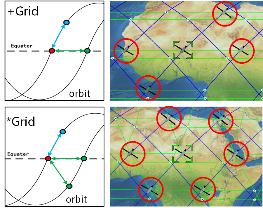
Figure 1: Structure of a mega-constellation network formed by different ISL patterns.The first row is the structure of the ‘+Grid’ mode, in which each satellite is adjacent to two sISLs, and the second row is the ‘*Grid’ mode, in which each satellite is connected to four sISLs.

Several existing works[5, 6, 7, 8] tried to model satellite matching problem and optimize the topology of novel constellations. However, these efforts has primarily focused on the constellation with limited scale, such as Iridium-like network. These focus ignores the impact of different ISL spanning patterns on the global network or the applicability to the emerging mega-constellations. In references[9, 10, 11, 12], authors have analyzed the performance of global mega-constellation network, considering a certain proposed ISL connectivity mode such as ‘+Grid’[10] or ‘xGrid’[12]. However, a conspicuous gap persists in the absence of a clear formulation regarding how the satellites connect to each other and an evaluation of network structures under various pattern configurations.

To reveal the structure characteristic of mega-constellation network formed by different ISL building configuration and its networking performance, we formulate the ISL spanning pattern and categorize the patterns into ‘+Grid’ and ‘*Grid’ modes based on the number of ISLs per satellite. We conduct evaluations under multiple constellations with varying ISL spanning patterns and satellite density. This allow us to validate the impact of structures formed by these patterns on the network performance. Based on comprehensive experiments, we propose two optimal patterns for the ‘+Grid’ and ‘*Grid’ modes, respectively. These patterns contribute to the best network performance in terms of multiple metrics. To the best of our knowledge, this work is the first to formulate ISL spanning patterns and apply them to LEO Mega-constellations. The structures of the network with different spanning patterns are shown in Fig.1.

The contributions of this paper can be summarized as follows:

• We formulate the ISL spanning patterns and apply them to mega-constellations, providing the visualizations of these structures;

• We evaluate the networks formed by various ISL spanning patterns using different metrics including path latency, stretch, capacity and throughput. Our evaluations enable us to identify the network structure with the optimal ISL spanning pattern.

II Model and Spanning Pattern Formulation

II-A Network Model

To address the temporal variations in the satellite networks, we denote an ordered time set as $\mathcal{T}=\{t_{1},t_{2},\cdots\}$. The network topology without encountering ISLs[13] can be considered unchanged between adjacent time stamps. $t_{i+1}-t_{i}$ represents the minimum time granularity of scenario change. Therefore, the network topology at each time stamp $t\in\mathcal{T}$ can be formulated as an undirected graph $\mathcal{G}^{t}=(\mathcal{V},\mathcal{E}^{t})$, where $\mathcal{V}$ is the set of network vertices (satellites) and $\mathcal{E}^{t}$ is the set of undirected edges ( including iISL, sISLs and eISLs).

The Walker[4] constellation, which provide uniform coverage around the Earth, is generally described as $T/P/F/i$, where $T$ is the total number of satellites, $P$ is the number of equally spaced planes, $F$ is the phase factor and $i$ is orbit inclination. The change for satellites between neighboring planes is equal to $F\times 360/T$. The value range of the phase factor is $F\in[0,P-1]$. When $F=F_{m}$, the phase bias between satellites in two adjacent orbits achieves maximum where:

$$F_{m}=\left\{\begin{aligned} P/2-1&,&P\text{~{}is~{}even.}\\ (P-1)/2&,&P\text{~{}is~{}odd.}\end{aligned}\right.$$ (1)

II-B ISL Spanning Pattern Formulation

Intra-orbit Links (iISL). Without considering orbital perturbations, each satellite in the same orbit (plane) follows the same direction and velocity. If a satellite establishes a link only with a neighbor satellite in the same orbit, the topology can be considered invariant. This is the only case of intra-orbit link in this paper.

Inter-orbit links (side links, sISL). Inter orbit links, i.e., the side links, refer to connections established between two satellites that move in the same direction but within side orbits.

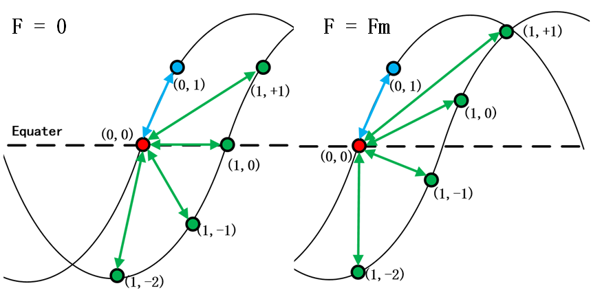
Figure 2: Possible sISLs (green) of satellite (0,0) in networks with $F=0$ and $F=F_{m}$.

The possible sISL between a satellite (red point) and its side-orbit satellites (green point) are shown in Fig.2, including both $F=0$ (left) and $F=F_{m}$ (right) cases. The satellite is denoted as a tuple $(n,f)$, where $n$ is orbit-number and $f$ is phase-number. We only consider establishing links with side orbit satellite having phase bias within {-2, -1, 0, 1}. Based on this criterion, we formulate the ISL spanning pattern as a phase bias set:

$$\mathcal{B}\subseteq\{-2,~{}-1,~{}0,~{}1\}$$ (2)

If each satellite is equipped with 4 ISLs, comprising 2 iISLs and 2 sISLs, the pattern corresponds to the ‘+Grid’ mode, as described in [10]. In this configuration, the number of elements in phase bias set is $\left\lVert\mathcal{B}\right\rVert=1$. Conversely, if each satellite has 6 ISLs, including 2 iISLs and 4 sISLs, the pattern is categorized as the ‘*Grid’ mode, and $\left\lVert\mathcal{B}\right\rVert=2$. Consequently, there are four distinct spanning patterns in the ‘+Grid’ mode, represented by $\mathcal{B}=\{1\}$, $\mathcal{B}=\{0\}$, $\mathcal{B}=\{-1\}$, and $\mathcal{B}=\{-2\}$, with a more concise notation of b1, b0, bm1, and bm2, respectively. Similarly, the ‘*Grid’mode encompasses six spanning patterns, which can be defined as $\mathcal{B}=\{1,0\}$, $\mathcal{B}=\{0,-1\}$, $\mathcal{B}=\{-1,-2\}$, $\mathcal{B}=\{1,-1\}$, $\mathcal{B}=\{1,-2\}$, and $\mathcal{B}=\{0,-2\}$, denoted as b10, b0m1, bm1m2, b1m1, b1m2 and b0m2, respectively. Consequently, the network configuration of these constellations is determined by the parameters $T/P/F/i$ and the phase bias set $\mathcal{B}$. It’s important to note that the number of transceivers on each satellite is constrained by cost considerations. Therefore scenarios involving satellites with more than four sISLs are not addressed in this paper.

III Network Evaluation Metrics

III-A ISL direction distribution

The phase factor $F$ and the bias set $\mathcal{B}$ play a crucial role in determining the ISL pattern, which inturn defines the global structure of the network. This results in ISLs with different directional distributions.

It is known that, the sISLs in $F=0,\mathcal{B}=\{0\}$ pattern run parallel to the equator, which is called Horizontal Ring[14]. This configuration effectively increases the connectivity of the network in the East-West direction[9]. In fact, directional connectivity reflects the distribution of ISLs over different directions, i.e., the higher the connectivity in a certain direction, the greater the proportion of ISLs within that angle, which will reduce the path zigzag in that direction and thus reduce the propagation latency.

In order to describe the directional connectivity of the constellation under different structures, we define the $\alpha$ as the angle between the ISL and Equator plane as:

$$\alpha=\frac{\pi}{2}-\arccos{(\frac{\mathbf{e}\cdot\mathbf{e}_{z}}{\|\mathbf{e}\|\cdot\|\mathbf{e}_{z}\|})}$$ (3)

where the $e_{z}$ is the normal vector of Equator plane, i.e., the rotation axis of Earth. We count the probability density function $h(\alpha)$ during time $\mathcal{T}$ as follows:

$$h^{\mathcal{T}}(\alpha)=\frac{\sum\limits_{\mathcal{T}}h^{t}(\alpha)}{\|\mathcal{T}\|}$$ (4)

III-B Propagation Latency and Stretch

For a specific network structure, we calculate the route between any two satellites within a period of time and derive the propagation latency:

$$latency=\frac{L_{prop}(p[s_{i},s_{j}])}{c},s_{i},s_{j}\in S,$$ (5)

where $L_{prop}(p[s_{i},s_{j}])$ is the propagation distance of routing path that from $s_{i}$ to $s_{j}$, $S$ is the set of satellites and $c$ is light speed.

We define the stretch as the ratio of the path propagation distance $L_{prop}$ and the geodesic distance $L_{geo}$ between the same satellites pairs[10], which is expressed as:

$$stretch=L_{prop}/L_{geo}$$ (6)

Given that the propagation speed of signal in an optical fiber is about $2c/3$, where $c$ is the speed of light, it can be inferred that if the $stretch\leq 1.5$, the path propagation latency in satellite network is lower than that in terrestrial fiber.

III-C Network Capacity and Throughput

Network capacity is contingent on the amount of data processed per second of satellites and data rate of ISLs in the networks. Under ideal situations, when both the capacity of satellites and ISLs (data rate) reach their maximum, the network capacity is determined by the lower of these two factors:

$$C(\mathcal{G}^{t})=\mathop{min}[\sum\limits_{e\in\mathcal{E}^{t}}C(e),\sum\limits_{v\in\mathcal{V}}C(v)]$$ (7)

where $e$ and $v$ represent the ISL and satellites, respectively. Since changes in network structure primarily impact ISL capacity, we assume that satellite capacity is infinite. Therefore, the network capacity is $C(\mathcal{G})=\sum\limits_{e_{i}\in\mathcal{E}}C(e_{i})$.

Network throughput is defined as the maximum flow of the graph spanned by the paths of multiple connections in the network at a given moment. Although the graph has multiple source nodes and sink nodes, its maximum flow problem can be solved by introducing a super source and a super sink node[15], and the throughput is calculated as follows:

$$\mathcal{T}(\mathcal{P}^{t})=\mathop{maxflow}[\mathcal{P}^{t},v_{src},v_{dst}]$$ (8)

where $\mathcal{P}$ represents the set of routing paths, $v_{src},v_{dst}$ is super source and source sink nodes, respectively. The link capacity of these super nodes to regular node is defined as infinity. Network throughput needs to consider the network loads and we define the loads as the number of connection paires. In most cases, throughput gradually reaches an optimal value as the load increases.

IV Simulation Study

In this section, we evaluate the satellite network performance affected by different network structures in terms of latency, path stretch, capacity and throughput. We illustrate the differences and latency variations of routing path between two same end point (located at Harbin and London) under different network structure of ‘+Grid’ mode. Besides, we evaluate network performance under structures spanned by both ‘+Grid’ and ‘*Grid’ patterns, and the optimal structures are also given. Furthermore, we evaluate network performance under different density constellations.

IV-A Path latency and stretch analysis

The left of Fig.3 shows the probability density function (Eq.4) of ISL direction. It illustrates that iISL is concentrated at $53^{\circ}$ (black line), which designs with expectations given the orbital inclination of $53^{\circ}$. Patterns b1,b0,bm1,bm2 exhibit distinct distributions, which makes the routing between the same end nodes dramatically different. For example, the routing of east-west terminals, in the $0^{\circ},~{}180^{\circ}$ link distribution more structure, can achieve lower latency. The right of Fig.3 shows the one-way propagation latency between Harbin and London under Dijkstra routing algorithm. The figure shows that compared to the ISL pattern of b1, bm1, and bm2, the routing path achieves the lowest delay and jitter under the structure formed by the b0 pattern.

This observation is attributed to the fact that London and Harbin share similar latitudes, resulting in ample connectivity from East to West. The routing paths of above patterns are shown in Fig.4.

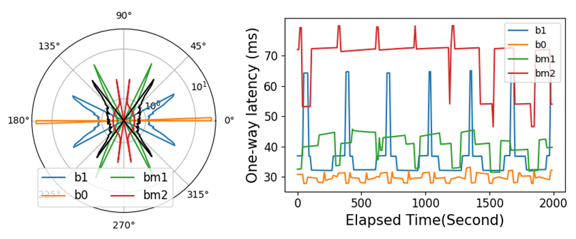
Figure 3: ISL direction distribution (left) and path latency (right) in varying patterns.

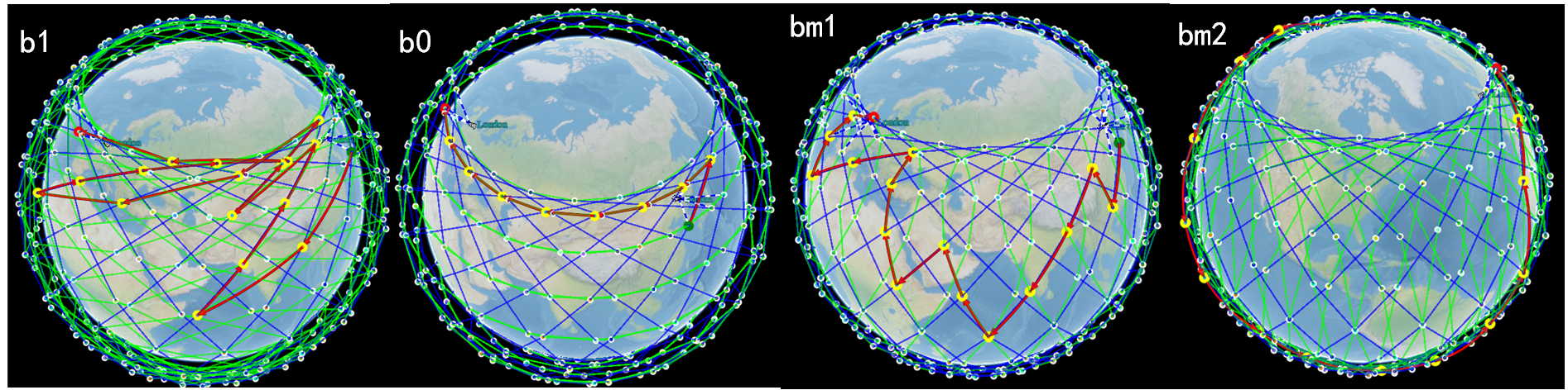
Figure 4: Routing paths between Harbin and London in varying patterns (F=0).

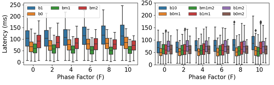
(a) Latency in ‘+Grid’ (left) and ‘*Grid’ (right) patterns.

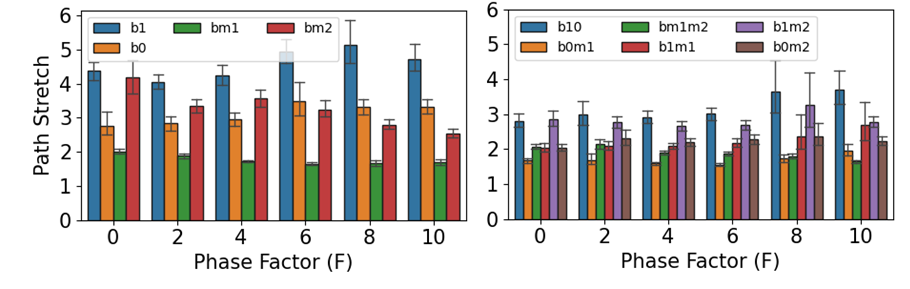
(b) Stretch in ‘+Grid’ (left) and ‘*Grid’ (right) patterns.

Figure 5: Latency and stretch distribution on networks with ‘+Grid’ and ‘*Grid’ mode patterns.

In our analysis of network structures defined by Inter-Satellite Link (ISL) patterns with varying phase factors, we noted that a more uniformly distributed connectivity proves to be more effective in minimizing the detour of routing path connections and, consequently, reducing latency. Fig.5 (a) displays the distribution of paths latencies generated by Dijkstra under different network structures between random satellites.

The left of Fig.5 (a) shows that the networks with bm1 pattern has achieved the lowest average latency over all phase factors, following the trend $T_{bm1}\leq T_{bm0}\leq T_{bm2}\leq T_{bm1}$. Within the structure of bm1, bm2 patterns, the latency is increases with the phase factor. In contrast, in the structures spanned by b1, b0 patterns, the latency is decreases with the phase factor. For the structure with bm1 pattern and $F=Fm$, the average latency is no more than 50ms and a maximum of no more than 80ms, which is only 40% of the worst-case (bm1 pattern at $F=10$). The right of Fig.5 (a) shows the latency of ‘*Grid’ structure that spanned by b10, b0m1, bm1m2, b1m1, b1m2 and b0m2 patterns. It is evident that the average latency is significantly reduced compared to the ‘+Grid’ structure. In structures spanned by bm1m2, b0m2 patterns, the latency decreases gradually with increasing phase factor while it remains relatively stable in b1m2 pattern. In the structures spanned by b10, b0m1, b1m1 patterns, however, the latency increases with increasing phase factor, where the b0m1 mode has the lowest latency at the same phase. It reaches its lowest at $F=0$, with an average of 47ms and a maximum of 70ms.

We have also evaluated the path stretch that given by 6 under different structures, which is shown in Fig.5 (b). Similarly, the structures in ‘+Grid’ mode that spanned by bm1 patterns achieve the best results over all phase factors. While in ‘*Grid’ mode, the structure that spanned by b0m1 pattern with $F=0$ achieved the best result compared with the others.

IV-B Capacity and throughput analysis

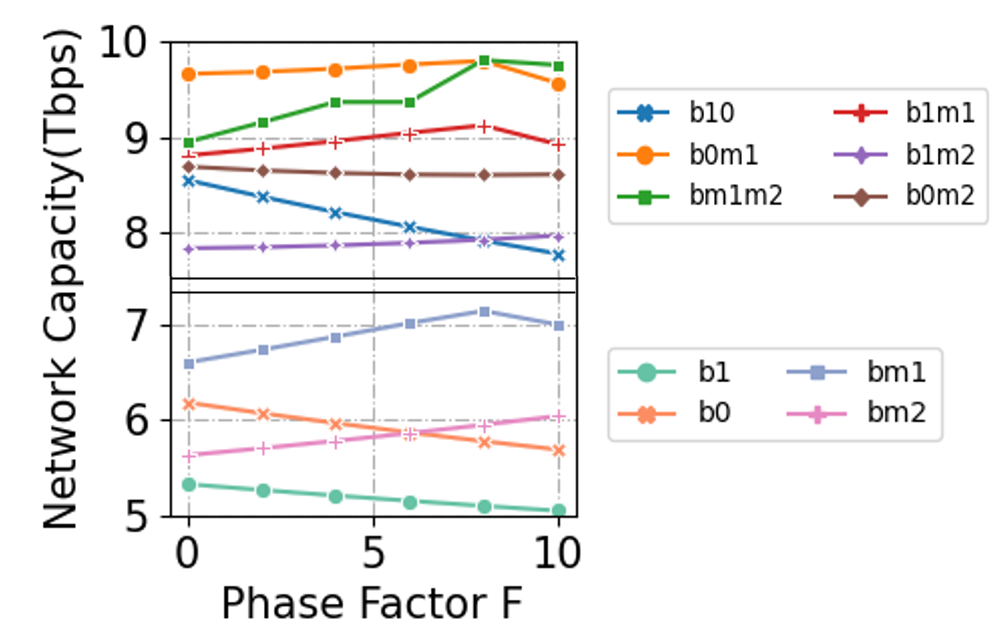
Figure 6: Capacity on ‘+Grid’ (left) and ‘*Grid’ (right) network structures.

The different ISL patterns result in varying link capacity due to different free space losses, thus affecting the network capacity differently. The Fig.6 illustrates how the network capacity changes for structures spanned by various ISL patterns. On the right side of Fig.6, the capacity decreases as $F$ increases for the b1, b0 patterns, while it increases for bm1 and bm2. The bm1 pattern outperforms others, reaching its maximum capacity of 7.2 Tbps at $F=8$. On the left side of Fig.6 (b), the capacity decreases as $F$ increases for the b10 pattern, while it increases for b1m1 and b1m2. The b0m1, b0m2, and b1m2 patterns show slow variation with changes in the phase factor, demonstrating more stability features. The b0m1 pattern stands out as superior to others, reaching its maximum capacity of 9.75 Tbps at $F=8$. Therefore, in most cases, bm1 links and b0m1 links represent the optimal structures, achieving the maximum network capacity. Compared to the ‘+Grid’ configuration, the ‘*Grid’ configuration shows a 37% increase in capacity.

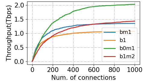
Figure 7: Network throughput in structures with $F=0$.

The throughput of different structured networks under different loads is shown in Fig.7. We selected several typical structures, bm1,b1,b0m1,b1m2 for evaluation. we generate 1000 random end-to-end pairs as the loads of network and calculate their paths under Dijkstra algorithm at each timestamp. In patterns of ‘+Grid’ mode, with a loads of 400 connections, the throughput of b1 and bm1 has converged to 1 Tbps and 1.35 Tbps, respectively. In patterns of ‘*Grid’ mode, the b1m2 and b0m1 structures, when the number of loads is around 800, the throughput starts to converge and reaches 1.35 Tbps and 2 Tbps, respectively. We observe that the ‘+Grid’ structures formed by bm1 patterns and ‘*Grid’ structures formed by b0m1 offer superior throughput while under the same routing scheme and loads.

In summary, bm1 is optimal pattern under $F=Fm$ in the ‘+Grid’ structures, while b0m1 is optimal pattern in the ‘*Grid’ structures.

IV-C Density analysis

Constellation networks of different density exhibit varying performance, where higher density satellites tend to have higher throughput and lower latency. Fig.8 depicts the distribution of path stretch and latency in structures formed by b0m1 pattern at $F=0$ with densities $10^{2}$, $20^{2}$, $30^{2}$ and $40^{2}$, respectively.

In Fig.8 (a), the network with $10^{2}$ density exhibits the worst results, with more than 80% of the paths having a stretch value of 2.9. In contrast, the other networks the value of about 1.6. Additionally, over 70% of the paths stretch in the networks of $20^{2}$, $30^{2}$ and $40^{2}$ is lower than 1.5, surpassing the performance of geodesic fiber transmission (black dash line). In Fig.8 (b), we observe that the maximum latency in network with $10^{2}$ density exceeds 120ms, whereas it remains below 80ms in networks with density  $20^{2}$ $30^{2}$ and $40^{2}$. It illustrates that compared to the $10^{2}$ network, the $20^{2}$ network reduces the average latency from 75ms to 50ms, marking approximately a 33% reduction. However, as the constellation size continues to grow, there is very limited improvement in the path latency and stretch, since the routing paths are getting approximate to the geodesic arc. Therefore, a network density of $20^{2}$ is sufficiently in the terms of path latency or stretch.

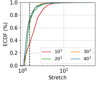
(a) Path stretch distribution.

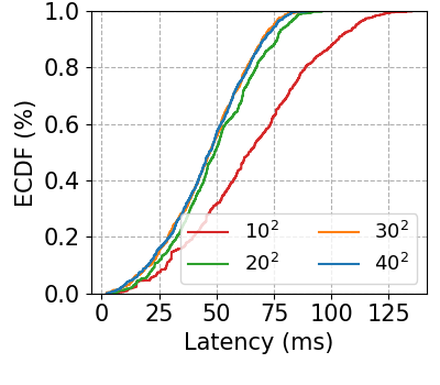
(b) Path latency distribution.

Figure 8: ECDF of path stretch and latency in network structures with density $10^{2},~{}20^{2},~{}30^{2},~{}40^{2}$.

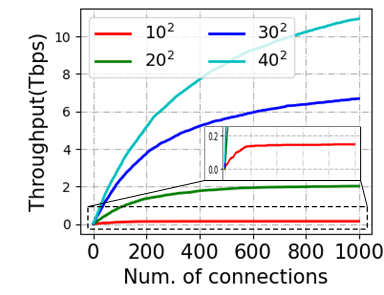
(a) Network throughputs.

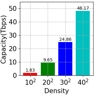
(b) Network capacity.

Figure 9: Network capacity and throughput in structures with density $10^{2},~{}20^{2},~{}30^{2},~{}40^{2}$.

We also provide the capacity and throughput among networks with different density. Fig.9 shows the throughput and capacity of networks with different densities under ‘*Grid’ mode spanned by b0m1 ISL pattern at $F=0$. It illustrates the network with $10^{2}$ density reaches the throughput maximum at 200 connections, achieving about 0.16 Tbps. In contrast, the $20^{2}$ network reaches the maximum at 600 connections. $30^{2}$ and $40^{2}$ networks do not reach the maximum at more than 1,000 connections. The theoretical capacity of $10^{2}$, $20^{2}$, $30^{2}$ and $40^{2}$ densities are 1.83 Tbps, 9.65 Tbps, 24.86 Tbps and 48.17 Tbps, respectively.

V Conclusion

This study addresses the challenges of determining optimal structure of LEO mega-constellation networks. We formulate the ISL spanning patterns, apply different patterns to mega-constellation and generate multiple structures. Through comprehensive experiments, we draw several conclusions: 1) In the case of utilizing the ‘+Grid’ mode, it is observed that the bm1 pattern offers the most optimal structure. To achieve the best latency or throughput, it is advisable to maximize the constellation phase factor. 2) In the case of utilizing the ‘*Grid’ mode, it is observed that the b0m1 pattern offers the most optimal structure. To achieve the latency or throughput, it is recommended to minimum the constellation phase factor. 3) Increasing the density of constellations can effectively improve the performance of the network, but the increase in latency is limited, and the density of more than $20^{2}$ is of little significance, while the more important thing is to improve the network capacity and throughput.

References

- [1] L. Space Exploration Holdings, “Spacex ka-band ngso constellation fcc filing sat-loa-20161115-00118,” http://licensing.fcc.gov.
- [2] F. C. Commision, FCC Grants OneWeb US Access for Broadband Satellite Constellation., https://docs.fcc.gov/public/attachments/DOC-345467A1.pdf, 2017.
- [3] T. Canada, SAT-MPL-20200526-00053, http://licensing.fcc.gov/myibfs/forwardtopublictabaction.do?filenumber=SATMPL2020052600053.
- [4] J. G. Walker, “Satellite constellations,” Journal of the British Interplanetary Society, vol. 37, p. 559, 1984.
- [5] Q. Chen, J. Guo, L. Yang, X. Liu, and X. Chen, “Topology virtualization and dynamics shielding method for leo satellite networks,” IEEE Communications Letters, vol. 24, no. 2, pp. 433–437, 2019.
- [6] I. Leyva-Mayorga, B. Soret, and P. Popovski, “Inter-plane inter-satellite connectivity in dense leo constellations,” IEEE Transactions on Wireless Communications, vol. 20, no. 6, pp. 3430–3443, 2021.
- [7] B. Soret, I. Leyva-Mayorga, and P. Popovski, “Inter-plane satellite matching in dense leo constellations,” in IEEE Global Communications Conference (GLOBECOM), 2019.
- [8] Z. Yan, G. Gu, K. Zhao, Q. Wang, G. Li, X. Nie, H. Yang, and S. Du, “Integer linear programming based topology design for gnsss with inter-satellite links,” IEEE Wireless Communications Letters, 2020.
- [9] M. Handley, “Delay is not an option: Low latency routing in space,” in Proceedings of the 17th ACM Workshop on Hot Topics in Networks, 2018, pp. 85–91.
- [10] D. Bhattacherjee and A. Singla, “Network topology design at 27,000 km/hour,” in Proceedings of the 15th International Conference on Emerging Networking Experiments And Technologies, 2019.
- [11] D. Bhattacherjee, “Towards performant networking from low-earth orbit,” Ph.D. dissertation, ETH Zurich, 2021.
- [12] J. Mclaughlin, J. Choi, and R. Durairajan, “ grid: A location-oriented topology design for leo satellites,” in Proceedings of the 1st ACM Workshop on LEO Networking and Communication, 2023.
- [13] W. Xiangtong, L. Wei, Y. Menglong, H. Songchen, and J. Zhiyun, “Enabling high-connectivity leo satellite networks via encountering inter-satellite links,” in IEEE Global Communications Conference (GLOBECOM), 2023.
- [14] E. Ekici, I. F. Akyildiz, and M. D. Bender, “Datagram routing algorithm for leo satellite networks,” in Proceedings IEEE INFOCOM 2000. Conference on Computer Communications. Nineteenth Annual Joint Conference of the IEEE Computer and Communications Societies (Cat. No. 00CH37064), 2000.
- [15] D. B. West et al., Introduction to graph theory. Prentice hall Upper Saddle River, 2001, vol. 2.