Distributed Stochastic Optimization under Heavy-Tailed Noises

Abstract

This paper studies the distributed optimization problem under the influence of heavy-tailed gradient noises. Here, a heavy-tailed noise $\xi$ means that the noise $\xi$ does not necessarily satisfy the bounded variance assumption, i.e., $E[\|\xi\|^{2}]\leq\nu^{2}$ for some positive constant $\nu$. Instead, it satisfies a more general assumption $E[\|\xi\|^{\delta}]\leq\nu^{\delta}$ for some $1<\delta\leq 2$. The commonly-used bounded variance assumption is a special case of the considered noise assumption. A typical example of this kind of noise is a Pareto distribution noise with tail index within (1,2], which has infinite variance. Despite that there has been several distributed optimization algorithms proposed for the heavy-tailed noise scenario, these algorithms need a centralized server in the network which collects the information of all clients. Different from these algorithms, this paper considers that there is no centralized server and the agents can only exchange information with neighbors in a communication graph. A distributed method combining gradient clipping and distributed stochastic subgradient projection is proposed. It is proven that when the gradient descent step-size and the gradient clipping step-size meet certain conditions, the state of each agent converges to the optimal solution of the distributed optimization problem with probability 1. The simulation results validate the algorithm.

I Introduction

I-A Distributed Optimization

Distributed optimization is a method of achieving optimization through cooperation among multiple agents, which can be used to solve large-scale optimization problems that are hard for centralized algorithms to cope with. The core idea of distributed optimization is to decompose a large problem into small problems and distribute the local objectives to multiple intelligent agents for solution. Compared with centralized optimization, distributed optimization overcomes the disadvantages of single point of failure, high computation and communication burden, and restrictions on scalability and flexibility [1]. Distributed optimization has a wide range of applications, such as machine learning [2], distributed economic dispatch problem of energy systems[3], and formation control problem in robotic systems [4].

I-B Distributed Stochastic Optimization

Different from deterministic optimization, stochastic optimization employs random factors to reach a solution to optimization problems. Stochastic optimization has wild applications in various fields. For example, the stochastic gradient descent (SGD) method has greatly participated in the progress of machine learning.

As an extension of distributed deterministic optimization to stochastic scenarios, distributed stochastic optimization has also attracted widespread attention. For instance, the authors in [5] presented a distributed stochastic subgradient projection algorithm tailored for convex optimization challenges. [6] introduced a distributed algorithm that relies on asynchronous step-sizes. [7] proposed a proximal primal-dual approach geared towards nonconvex and nonsmooth problems. [8] examined the high-probability convergence of distributed stochastic optimization.

I-C Heavy-Tailed Noise

Most of the above literature on stochastic optimization assume that the variance of the random variable is bounded. Despite that this is a mild assumption which covers many noises such as Gaussian noises, there are still many noises that do not satisfy this condition. For example, the Pareto distribution and the $\alpha$-stable Levy distribution [9]. Heavy-tailed noises has been recently observed in many machine learning systems [9, 10, 11, 12, 13]. For example, in [9], it was found that an attention training model on Wikipedia can generate heavy-tailed noises. Moreover, it is shown that the traditional SGD method may diverge when the noise is heavy-tailed [9, 10].

I-D Contributions

In this work, we study the distributed stochastic optimization algorithm under heavy-tailed gradient noises using neighboring agents' information exchange only. The main contributions of this paper are listed as follows:

1) We design a distributed updating law to deal with the stochastic optimization problem under heavy-tailed noises. Strict proof is given to show that under some mild parameter conditions, the state of each agent converges to the optimal solution with probability 1.

2) Compared with the existing distributed stochastic optimization works, e.g., [5, 6, 14, 15, 16, 7], our algorithm allows heavy-tailed noises that satisfy $E[\|\xi\|^{\delta}]\leq\nu^{\delta}$ for some $1<\delta\leq 2$ and positive constant $\nu$, which generalizes the commonly used assumption $E[\|\xi\|^{2}]\leq\nu^{2}$.

3) Compared with the existing literature on heavy-tailed noises, e.g., [9, 17, 18, 19, 10, 20, 21, 22], our algorithm is distributed in the sense that there is no central server and the agents can only exchange information via a strongly connected communication graph. Note that despite that [10, 20, 21, 22] studied heavy-tailed noises in a distributed setting, these algorithms require a central server [10, 21, 22] or the agents require the states of all the other agents at some time instant [20]. These works are not related to multi-agent consensus while our work is related to consensus and graph theory.

I-E Organization

The rest of this paper is organized as follows: In Section II, notations and preliminary knowledge are given. In Section III, the studied distributed optimization problem is formulated. In Section IV, a distributed updating law is proposed for each agent based on gradient clipping and distributed stochastic subgradient projection method. The almost sure convergence to the optimal solution is proven. In Section V, a numerical example is given to illustrate the effectiveness and efficiency of the proposed algorithm. Finally, in Section VI, we conclude the paper.

II Notations and Preliminaries

Throughout this paper, $0$ represents a zero vector with an appropriate dimension or scalar zero. $\mathbb{R}$ and $\mathbb{R}^{N}$ represent the real number set and the $N$-dimensional real vector set, respectively. $\left|\cdot\right|$ is the absolute value of a scalar, and $\left\|\cdot\right\|$ is the 2-norm of a vector. The ``inf" represent the infimum of a sequence. $P_{\Omega}[\cdot]$ is the Euclidean projection of a vector to the space $\Omega$. $[e]_{i}$ is the $i$-th element of a vector $e$. $[A]_{i,j}$ is the element in the $i$-th row and the $j$-th column of a matrix $A$. $\min\{a,b\}$ represents the minimum of $a$ and $b$. $E[\cdot]$ is the expectation of a variable.

Lemma 1

[5] For scalars $\beta_{1},\ldots,\beta_{N}\geq 0$ where $\sum_{i=1}^{N}\beta_{i}=1$ and vectors $v_{1},\ldots,v_{N}\in\mathbb{R}^{n}$, the following conclusion holds:

$$\left\|\sum_{i=1}^{N}\beta_{i}v_{i}\right\| \leq\sum_{i=1}^{N}\beta_{i}\left\|v_{i}\right\|,$$

$$\left\|\sum_{i=1}^{N}\beta_{i}v_{i}\right\|^{2} \leq\sum_{i=1}^{N}\beta_{i}\|v_{i}\|^{2}.$$ (1)

Lemma 2

(Lemma 3.1 of [5]) Let $\gamma_{k}$ be a scalar sequence. (1) If $\lim_{k\rightarrow+\infty}\gamma_{k}=\gamma$ and $0<\beta<1$, then $\lim_{k\rightarrow+\infty}\sum_{\ell=0}^{k}\beta^{k-\ell}\gamma_{\ell}=\frac{\gamma}{1-\beta}.$ (2) If $\gamma_{k}\geq 0$ for all $k$, $\sum_{k=0}^{+\infty}\gamma_{k}<\infty$ and $0<\beta<1$, then $\sum_{k=0}^{+\infty}\left(\sum_{\ell=0}^{k}\beta^{k-\ell}\gamma_{\ell}\right)<\infty$.

III Problem Formulation

Consider a multi-agent system comprised of $N>1$ agents. The agents cooperate to solve the following optimization problem

$$\min_{\theta\in\Omega}f(\theta)=\sum_{i=1}^{N}f_{i}(\theta),$$ (2)

where $\theta\in\Omega\subset\mathbb{R}^{n}$ is the decision variable, $f(\theta)$ is the global objective function, $f_{i}(\theta)$ is the local objective function in agent $i$, and $\Omega$ is the local constraint set.

Suppose that each agent can only get information from its neighbors via a communication graph $\mathcal{G}_{N}:=\{\mathcal{V}_{N},\mathcal{E}_{N}\}$ where $\mathcal{V}_{N}=\{1,\cdots,N\}$ is the node set, and $\mathcal{E}_{N}\subset\mathcal{V}_{N}\times\mathcal{V}_{N}$ is the edge set. Let $A$ be the adjacency matrix of $\mathcal{G}_{N}$.

Assumption 1

[5] The graph $\mathcal{G}_{N}$ is strongly connected. The adjacency matrix $A$ is doubly stochastic, i.e., $\sum_{i=1}^{N}a_{i,j}=\sum_{j=1}^{N}a_{i,j}=1$. There exists a scalar $0<\eta<1$ such that $a_{i,j}\geq\eta$ when $j\in\mathcal{N}_{i}$.

Assumption 2

The constraint set $\Omega$ is nonempty, convex and compact.

Assumption 3

$f_{i}(\theta)$ is strongly convex in $\theta$, i.e., there exists a modulus $\mu>0$ such that $f(\mathbf{z_{2}})-f(\mathbf{z_{1}})-(\nabla f(\mathbf{z_{1}}))^{\top}(\mathbf{z_{2}}-\mathbf{z_{1}})\geq\mu\|\mathbf{z_{1}}-\mathbf{z_{2}}\|^{2}$ for any $\mathbf{z_{1}},\mathbf{z_{2}}\in\Omega$. Moreover, $f_{i}(\theta)$ is continuously differentiable.

Under Assumptions 2 and 3, there exists a unique optimal solution $\theta^{*}$.

Remark 1

Assumptions 1, 2, 3 are all commonly-used assumptions in the literature. For example, Assumption 1 is used in [5, 16], Assumption 2 is used in [23, 9], and Assumption 3 is used in [24, 16].

IV Algorithm Design

The distributed updating law for agent $i$ is designed as

$$x_{i,k+1}=P_{\Omega}\left[v_{i,k}-\alpha_{k}\hat{g}_{i,k}(v_{i,k})\right],x_{i,0}\in\Omega$$ (3)

where

$$v_{i,k}=\sum_{j=1}^{N}a_{i,j}x_{j,k},$$ (4)

and

$$\hat{g}_{i,k}(v_{i,k}) =\min\left\{1,\frac{\tau_{k}}{\|g_{i,k}(v_{i,k})\|}\right\}g_{i,k}(v_{i,k}),$$

$$g_{i,k}(v_{i,k}) =\nabla f_{i}(v_{i,k})+\xi_{i,k}.$$ (5)

In (3)-(5), $\alpha_{k}$ and $\tau_{k}$ are two positive sequences determined later, $\xi_{i,k}$ is the random variable of agent $i$ at step $k$.

Let $\mathcal{F}_{k}$ be the $\delta$-algebra generated by the random variables from $0$ to $k-1$.

The following assumptions on the noises are made to facilitate the subsequent analysis.

Assumption 4

[9] (Bounded $\alpha$-Moment) There exists two positive constants $\delta$ and $\nu$ with $\delta\in(1,2]$ and $\nu>0$ such that $E[\|\xi_{i,k}\|^{\delta}|\mathcal{F}_{k}]\leq\nu^{\delta}$ with probability 1.

Remark 2

When $\delta=2$, Assumption 4 reduces to a standard assumption $E[\|\xi_{i,k}\|^{2}|\mathcal{F}_{k}]\leq\nu^{2}$. Note that a heavy-tailed noise satisfying Assumption 4 may violate the bounded variance assumption. See Section V for an example.

Assumption 5

(Unbiased Local Gradient Estimator) $E[\xi_{i,k}|\mathcal{F}_{k}]=0$ with probability 1.

Remark 3

The algorithm proposed in (3)-(5) is motivated by the GClip algorithm for a centralized convex optimization problem with heavy-tailed noises proposed in [9] and the distributed stochastic subgradient projection algorithm proposed for a distributed convex optimization problem with standard noises in [5].

Remark 4

In (3)-(5), all agents use the same gradient decent step-size and gradient clipping step-size. Thus, the algorithm is not ``fully distributed". In fact, this hypothesis is common in the existing distributed optimization literature. This work is still novel compared with the existing algorithms on heavy-tailed noises since the state exchange is distributed.

Let $b_{i,k}=\hat{g}_{i,k}-\nabla f_{i}(v_{i,k})$ and $B_{i,k}=E[b_{i,k}|\mathcal{F}_{k}]=E[\hat{g}_{i,k}|\mathcal{F}_{k}]-\nabla f_{i}(v_{i,k})$ .

Based on Assumption 2, there exists a positive scalar $C_{0}$ such that $\|\nabla f_{i}(\theta)\|\leq C_{0}$ for all $\theta\in\Omega$.

Based on the definition of $v_{i,k}$ and Assumption 1, $v_{i,k}\in\Omega$ for all $k\geq 0$.

Thus, $\|\nabla f_{i}(v_{i,k})\|\leq C_{0}$ for all $k\geq 0$.

Based on the above analysis, we can arrive at the following conclusion.

Lemma 3

Suppose that Assumptions 4 and 5 hold and $\tau_{k}\geq 2C_{0}$. Then, for all $i$, we have $\|B_{i,k}\|\leq(2\nu)^{\delta}\tau_{k}^{1-\delta}$ with probability 1.

Proof:

The proof is similar to Lemma 5.1 of [25]. For the completeness of this work, we put it here. Define

$$\chi=\mathbb{I}_{\{\|g_{i,k}\|>\tau_{k}\}}=\bigg{\{}\begin{array}[]{ll}1,&\text{ if }\|g_{i,k}\|>\tau_{k},\\ 0,&\text{ otherwise,}\end{array}\ \quad$$ (6)

and

$$\varepsilon=\mathbb{I}_{\{\|\xi_{i,k}\|>\frac{\tau_{k}}{2}\}}=\bigg{\{}\begin{array}[]{ll}1,&\text{ if }\|\xi_{i,k}\|>\frac{\tau_{k}}{2},\\ 0,&\text{ otherwise.}\end{array}\ \quad$$ (7)

Since $\tau_{k}\geq 2C_{0}$, $\|g_{i,k}\|\leq\frac{\tau_{k}}{2}+\|\xi_{i,k}\|$. Thus, $\varepsilon\geq\chi$. Since $\hat{g}_{i,k}=\min\{1,\frac{\tau_{k}}{\|g_{i,k}\|}\}g_{i,k}=\chi\frac{\tau_{k}}{\|g_{i,k}\|}g_{i,k}+(1-\chi)g_{i,k}$ and based on Assumption 5,

$$\|B_{i,k}\|= \bigg{\|}E\bigg{[}\left(g_{i,k}+\chi\left(\frac{\tau_{k}}{\|g_{i,k}\|}-1\right)g_{i,k}\right)|\mathcal{F}_{k}\bigg{]}$$

$$-\nabla f_{i}(v_{i,k})\bigg{\|}$$

$$= \left\|E\left[\left(\chi\left(\frac{\tau_{k}}{\|g_{i,k}\|}-1\right)g_{i,k}\right)|\mathcal{F}_{k}\right]\right\|$$

$$\leq E\left[\left(\chi\left|\frac{\tau_{k}}{\|g_{i,k}\|}-1\right|\left\|g_{i,k}\right\|\right)|\mathcal{F}_{k}\right]$$

$$= E\left[\chi\left(1-\frac{\tau_{k}}{\|g_{i,k}\|}\right)\|g_{i,k}\||\mathcal{F}_{k}\right]$$

$$\leq E\left[\chi\|g_{i,k}\||\mathcal{F}_{k}\right]$$

$$\leq E\left[\varepsilon\|g_{i,k}\||\mathcal{F}_{k}\right]$$

$$\leq E\left[\left(\varepsilon\|\xi_{i,k}\|+\varepsilon\|\nabla f_{i}(v_{i,k})\|\right)|\mathcal{F}_{k}\right]$$ (8)

with probability 1, where we used Jensen's inequality and the convexity of the norm.

Based on Holder's inequality for conditional expectation,

$$\|B_{i,k}\|\leq \left(E\left[\|\xi_{i,k}\|^{\delta}|\mathcal{F}_{k}\right]\right)^{\frac{1}{\delta}}\left(E\left[\varepsilon^{\frac{\delta}{\delta-1}}|\mathcal{F}_{k}\right]\right)^{\frac{\delta-1}{\delta}}$$

$$+\frac{\tau_{k}}{2}E[\varepsilon|\mathcal{F}_{k}]$$

$$\leq \nu\left(E\left[\varepsilon^{\frac{\delta}{\delta-1}}|\mathcal{F}_{k}\right]\right)^{\frac{\delta-1}{\delta}}+\frac{\tau_{k}}{2}E[\varepsilon|\mathcal{F}_{k}]$$

$$= \nu\left(E[\varepsilon|\mathcal{F}_{k}]\right)^{\frac{\delta-1}{\delta}}+\frac{\tau_{k}}{2}E[\varepsilon|\mathcal{F}_{k}]$$ (9)

with probability 1.

Based on the Markov's inequality for conditional expectation,

$$E[\varepsilon|\mathcal{F}_{k}] =P(\|\xi_{i,k}\|>\frac{\tau_{k}}{2}|\mathcal{F}_{k})$$

$$=P(\|\xi_{i,k}\|^{\delta}>\frac{\tau_{k}^{\delta}}{2^{\delta}}|\mathcal{F}_{k})$$

$$\leq\frac{E\left[\|\xi_{i,k}\|^{\delta}|\mathcal{F}_{k}\right]}{\frac{\tau_{k}^{\delta}}{2^{\delta}}}$$

$$\leq(2\nu)^{\delta}\tau_{k}^{-\delta}$$ (10)

with probability 1.

Then, $\|B_{i,k}\|\leq\nu(2\nu)^{\delta-1}\tau_{k}^{1-\delta}+\frac{1}{2}(2\nu)^{\delta}\tau_{k}^{1-\delta}=(2\nu)^{\delta}\tau_{k}^{1-\delta}$ with probability 1. ∎

The following lemma can be directly obtained from Lemma 3.2 of [5].

Lemma 4

Under Assumption 1, for any $k>0$, the following inequality holds:

$$\left|[A^{k}]_{i,j}-\frac{1}{N}\right|\leq\theta\beta^{k},$$ (11)

where $\theta=\left(1-\frac{\eta}{4N^{2}}\right)^{-2}$, and $\beta=\left(1-\frac{\eta}{4N^{2}}\right)^{\frac{1}{Q}}$. Here, $\eta$ was defined in Assumption 1 and $Q$ is the number of edges in graph $\mathcal{G}_{N}$. $[A^{k}]_{i,j}$ is the element of the $i$-th row and $j$-th column of $A^{k}$.

Based on the above lemmas, the following conclusion holds.

Theorem 1

Suppose that Assumptions 1-5 hold, and the parameters $\alpha_{k}$ and $\tau_{k}$ satisfy the following condition:

$$\sum_{k=0}^{+\infty}\alpha_{k}=\infty,\sum_{k=0}^{+\infty}\alpha_{k}^{2}<+\infty,$$ (12)

$$\tau_{k}\geq 2C_{0},\lim_{k\rightarrow+\infty}\alpha_{k}\tau_{k}=0,$$ (13)

$$\sum_{k=0}^{+\infty}\alpha_{k}^{2}\tau_{k}^{2}<+\infty,\sum_{k=0}^{+\infty}\alpha_{k}\tau_{k}^{2-2\delta}<+\infty,$$ (14)

where $C_{0}$ is a constant satisfying $\|\nabla f_{i}(\theta)\|\leq C_{0}$ for all $\theta\in\Omega$. Then, $x_{i,k}$ converges to the unique optimal solution $\theta^{*}$ with probability 1.

Proof:

Define

$$y_{k}=\frac{1}{N}\sum_{i=1}^{N}x_{i,k}\quad\text{ for all }k$$ (15)

and

$$p_{i,k+1}=x_{i,k+1}-v_{i,k}=x_{i,k+1}-\sum_{j=1}^{N}a_{i,j}x_{j,k}.$$ (16)

By (15) and (16), we have

$$y_{k+1} =\frac{1}{N}\sum_{i=1}^{N}\left(\sum_{j=1}^{N}a_{i,j}x_{j,k}+p_{i,k+1}\right)$$

$$=\frac{1}{N}\left(\sum_{j=1}^{N}\left(\sum_{i=1}^{N}a_{i,j}\right)x_{j,k}+\sum_{i=1}^{N}p_{i,k+1}\right)$$

$$=\frac{1}{N}\left(\sum_{j=1}^{N}x_{j,k}+\sum_{i=1}^{N}p_{i,k+1}\right)$$

$$=y_{k}+\frac{1}{N}\sum_{i=1}^{N}p_{i,k+1},$$ (17)

where we used Assumption 1.

Then,

$$y_{k+1} =y_{0}+\frac{1}{N}\sum_{\ell=1}^{k+1}\sum_{i=1}^{N}p_{i,\ell}$$

$$=\frac{1}{N}\sum_{i=1}^{N}x_{i,0}+\frac{1}{N}\sum_{\ell=1}^{k+1}\sum_{i=1}^{N}p_{i,\ell}$$

$$=\frac{1}{N}\sum_{j=1}^{N}x_{j,0}+\frac{1}{N}\sum_{\ell=1}^{k+1}\sum_{j=1}^{N}p_{j,\ell}.$$ (18)

Let $\mathbf{x}_{k}=[x_{1,k}^{\top},\cdots,x_{N,k}^{\top}]^{\top}$, $\mathbf{p}_{k}=[p_{1,k}^{\top},\cdots,p_{N,k}^{\top}]^{\top}$, $\tilde{A}=A\otimes I_{n}$, then (16) can be written as

$$\mathbf{p}_{k+1}=\mathbf{x}_{k+1}-\tilde{A}\mathbf{x}_{k},$$ (19)

which implies that

$$\mathbf{x}_{k+1} =\mathbf{p}_{k+1}+\tilde{A}\mathbf{x}_{k}$$

$$=\mathbf{p}_{k+1}+\tilde{A}(\mathbf{p}_{k}+\tilde{A}\mathbf{x}_{k-1})$$

$$=\sum_{\ell=0}^{k}\tilde{A}^{\ell}\mathbf{p}_{k+1-\ell}+\tilde{A}^{k+1}\mathbf{x}_{0}$$

$$=\sum_{\ell=1}^{k+1}\tilde{A}^{k+1-\ell}\mathbf{p}_{\ell}+\tilde{A}^{k+1}\mathbf{x}_{0},$$ (20)

where in the last step we use $k+1-\ell$ to replace $\ell$, and $\tilde{A}^{0}:=I_{Nn}$.

Thus,

$$x_{i,k+1} =\sum_{\ell=1}^{k+1}\sum_{j=1}^{N}[A^{k+1-\ell}]_{i,j}p_{j,\ell}+\sum_{j=1}^{N}[A^{k+1}]_{i,j}x_{j,0},$$ (21)

where $A^{0}\triangleq I_{N}$.

Based on (3),(16) and the non-expansive property of the projection operator,

$$\|p_{i,k+1}\| =\|P_{\Omega}\left[v_{i,k}-\alpha_{k}\hat{g}_{i,k}\right]-v_{i,k}\|$$

$$\leq\alpha_{k}\|\hat{g}_{i,k}\|$$

$$\leq\alpha_{k}\tau_{k}.$$ (22)

By (18) and (21), we have

$$\|y_{k+1}-x_{i,k+1}\| =\bigg{\|}\sum_{j=1}^{N}\left(\frac{1}{N}-[A^{k+1}]_{i,j}\right)x_{j,0}$$

$$+\frac{1}{N}\sum_{\ell=1}^{k+1}\sum_{j=1}^{N}p_{j,\ell}-\sum_{\ell=1}^{k+1}\sum_{j=1}^{N}[A^{k+1-\ell}]_{i,j}p_{j,\ell}\bigg{\|}$$

$$=\bigg{\|}\sum_{j=1}^{N}\left(\frac{1}{N}-[A^{k+1}]_{i,j}\right)x_{j,0}$$

$$+\frac{1}{N}\sum_{\ell=1}^{k}\sum_{j=1}^{N}p_{j,\ell}-\sum_{\ell=1}^{k}\sum_{j=1}^{N}[A^{k+1-\ell}]_{i,j}p_{j,\ell}$$

$$+\frac{1}{N}\sum_{j=1}^{N}p_{j,k+1}-p_{i,k+1}\bigg{\|}$$

$$\leq\sum_{j=1}^{N}\left|\frac{1}{N}-[A^{k+1}]_{i,j}\right|\|x_{j,0}\|$$

$$+\sum_{\ell=1}^{k}\sum_{j=1}^{N}\left|\frac{1}{N}-[A^{k+1-\ell}]_{i,j}\right|\|p_{j,\ell}\|$$

$$+\frac{1}{N}\sum_{j=1}^{N}\|p_{j,k+1}\|+\|p_{i,k+1}\|$$

$$\leq N\theta\beta^{k+1}C_{1}+N\sum_{\ell=1}^{k}\theta\beta^{k+1-\ell}\alpha_{\ell-1}\tau_{\ell-1}$$

$$+2\alpha_{k}\tau_{k},$$ (23)

where in the last step we used Lemma 4 and (22), and $C_{1}$ is a constant satisfying $\|x_{j,0}\|\leq C_{1}$ for all $j\in\mathcal{V}_{N}$.

For any $z\in\Omega$, based on the non-expansive property and the definition of $b_{i,k}$,

$$\|x_{i,k+1}-z\|^{2}= \|P_{\Omega}\left[v_{i,k}-\alpha_{k}\hat{g}_{i,k}\right]-z\|^{2}$$

$$\leq \|v_{i,k}-\alpha_{k}\hat{g}_{i,k}-z\|^{2}$$

$$= \|v_{i,k}-z\|^{2}-2\alpha_{k}\hat{g}_{i,k}^{\top}\left(v_{i,k}-z\right)$$

$$+\alpha_{k}^{2}\|\hat{g}_{i,k}\|^{2}$$

$$= \|v_{i,k}-z\|^{2}-2\alpha_{k}b_{i,k}^{\top}\left(v_{i,k}-z\right)$$

$$-2\alpha_{k}\nabla f_{i}(v_{i,k})^{\top}\left(v_{i,k}-z\right)$$

$$+\alpha_{k}^{2}\|\hat{g}_{i,k}\|^{2}$$

$$\leq (1-\mu\alpha_{k})\|v_{i,k}-z\|^{2}$$

$$-2\alpha_{k}(f_{i}(v_{i,k})-f_{i}(z))$$

$$-2\alpha_{k}b_{i,k}^{\top}\left(v_{i,k}-z\right)$$

$$+\alpha_{k}^{2}\tau_{k}^{2},$$ (24)

where in the last step we used the strong convexity of $f_{i}$ in Assumption 3.

Based on Lemma 1 and Assumption 1, we have

$$\sum_{i=1}^{N}\|v_{i,k+1}-z\|^{2} =\sum_{i=1}^{N}\bigg{\|}\sum_{j=1}^{N}a_{i,j}x_{j,k+1}-z\bigg{\|}^{2}$$

$$\leq\sum_{i=1}^{N}\sum_{j=1}^{N}a_{i,j}\|x_{j,k+1}-z\|^{2}$$

$$=\sum_{j=1}^{N}\sum_{i=1}^{N}a_{i,j}\|x_{j,k+1}-z\|^{2}$$

$$=\sum_{j=1}^{N}\|x_{j,k+1}-z\|^{2}.$$ (25)

Then, based on (24) and (24),

$$\sum_{i=1}^{N}\|v_{i,k+1}-z\|^{2}\leq (1-\mu\alpha_{k})\sum_{i=1}^{N}\|v_{i,k}-z\|^{2}$$

$$-2\alpha_{k}\sum_{i=1}^{N}(f_{i}(v_{i,k})-f_{i}(z))$$

$$-2\alpha_{k}\sum_{i=1}^{N}b_{i,k}^{\top}\left(v_{i,k}-z\right)$$

$$+N\alpha_{k}^{2}\tau_{k}^{2}.$$ (26)

Based on Lemma 1 and Assumption 3,

$$f_{i}\left(v_{i,k}\right)-f_{i}(z)= \left(f_{i}\left(v_{i,k}\right)-f_{i}\left(y_{k}\right)\right)$$

$$+\left(f_{i}\left(y_{k}\right)-f_{i}(z)\right)$$

$$\geq -\|\nabla f_{i}\left(v_{i,k}\right)\|\|y_{k}-v_{i,k}\|$$

$$+\left(f_{i}\left(y_{k}\right)-f_{i}(z)\right)$$

$$= -\|\nabla f_{i}\left(v_{i,k}\right)\|\bigg{\|}y_{k}-\sum_{j=1}^{N}a_{i,j}x_{j,k}\bigg{\|}$$

$$+\left(f_{i}\left(y_{k}\right)-f_{i}(z)\right)$$

$$\geq -\|\nabla f_{i}\left(v_{i,k}\right)\|\sum_{j=1}^{N}a_{i,j}\|y_{k}-x_{j,k}\|$$

$$+\left(f_{i}\left(y_{k}\right)-f_{i}(z)\right).$$ (27)

Thus, based on Assumption 1,

$$\sum_{i=1}^{N}(f_{i}\left(v_{i,k}\right)-f_{i}(z))$$

$$\geq -\sum_{i=1}^{N}\|\nabla f_{i}\left(v_{i,k}\right)\|\sum_{j=1}^{N}a_{i,j}\|y_{k}-x_{j,k}\|$$

$$+\sum_{i=1}^{N}\left(f_{i}\left(y_{k}\right)-f_{i}(z)\right)$$

$$\geq -C_{0}\sum_{i=1}^{N}\sum_{j=1}^{N}a_{i,j}\|y_{k}-x_{j,k}\|$$

$$+\sum_{i=1}^{N}\left(f_{i}\left(y_{k}\right)-f_{i}(z)\right)$$

$$= -C_{0}\sum_{j=1}^{N}\|y_{k}-x_{j,k}\|+\sum_{i=1}^{N}\left(f_{i}\left(y_{k}\right)-f_{i}(z)\right).$$ (28)

Then, based on (28), the inequality (26) can be written as

$$\sum_{i=1}^{N}\|v_{i,k+1}-z\|^{2}\leq (1-\mu\alpha_{k})\sum_{i=1}^{N}\|v_{i,k}-z\|^{2}$$

$$+2C_{0}\alpha_{k}\sum_{j=1}^{N}\|y_{k}-x_{j,k}\|$$

$$-2\alpha_{k}\left(f\left(y_{k}\right)-f(z)\right)$$

$$-2\alpha_{k}\sum_{i=1}^{N}b_{i,k}^{\top}\left(v_{i,k}-z\right)$$

$$+N\alpha_{k}^{2}\tau_{k}^{2}.$$ (29)

Taking the $\sigma$-algebra of (29) and letting $z=\theta^{*}$ gives

$$\sum_{i=1}^{N}E[\|v_{i,k+1}-\theta^{*}\|^{2}|\mathcal{F}_{k}]\leq (1-\mu\alpha_{k})\sum_{i=1}^{N}\|v_{i,k}-\theta^{*}\|^{2}$$

$$+2C_{0}\alpha_{k}\sum_{j=1}^{N}\|y_{k}-x_{j,k}\|$$

$$-2\alpha_{k}\left(f\left(y_{k}\right)-f(\theta^{*})\right)$$

$$-2\alpha_{k}\sum_{i=1}^{N}B_{i,k}^{T}\left(v_{i,k}-\theta^{*}\right)$$

$$+N\alpha_{k}^{2}\tau_{k}^{2}.$$ (30)

Based on Lemma 3 and utilizing Young's inequality to the last but one term, we have

$$\sum_{i=1}^{N}E[\|v_{i,k+1}-\theta^{*}\|^{2}|\mathcal{F}_{k}]\leq \sum_{i=1}^{N}\|v_{i,k}-\theta^{*}\|^{2}$$

$$+2C_{0}\alpha_{k}\sum_{j=1}^{N}\|y_{k}-x_{j,k}\|$$

$$-2\alpha_{k}\left(f\left(y_{k}\right)-f(\theta^{*})\right)$$

$$+\frac{N}{\mu}\alpha_{k}(2\nu)^{2\delta}\tau_{k}^{2-2\delta}$$

$$+N\alpha_{k}^{2}\tau_{k}^{2}$$ (31)

with probability 1.

According to (23), it can be obtained that

$$\sum_{k=0}^{+\infty}\alpha_{k}\sum_{j=1}^{N}\|y_{k}-x_{j,k}\| \leq N^{2}\theta C_{1}\sum_{k=0}^{+\infty}\alpha_{k}\beta^{k+1}$$

$$+N^{2}\theta\sum_{k=0}^{+\infty}\alpha_{k}\sum_{\ell=1}^{k}\beta^{k+1-\ell}\alpha_{\ell-1}\tau_{\ell-1}$$

$$+2N\sum_{k=0}^{+\infty}\alpha_{k}^{2}\tau_{k}.$$ (32)

Since $\sum_{k=0}^{+\infty}\alpha_{k}^{2}<+\infty$, $\alpha_{k}$ is bounded. According to the definition of $\beta$ in Lemma 4, $0<\beta<1$. Then, $N^{2}\theta C_{1}\sum_{k=0}^{+\infty}\alpha_{k}\beta^{k+1}$ is bounded.

Since $\sum_{k=0}^{+\infty}\alpha_{k}^{2}\tau_{k}^{2}<+\infty$, based on Lemma 2 (2), we have

$$N^{2}\theta\sum_{k=0}^{+\infty}\alpha_{k}\sum_{\ell=1}^{k}\beta^{k+1-\ell}\alpha_{\ell-1}\tau_{\ell-1}$$

$$\leq \frac{N^{2}\theta}{2}\sum_{k=0}^{+\infty}\sum_{\ell=1}^{k}\beta^{k+1-\ell}(\alpha_{k}^{2}+\alpha_{\ell-1}^{2}\tau_{\ell-1}^{2})$$

$$\leq \frac{N^{2}\theta}{2}\sum_{k=0}^{+\infty}\alpha_{k}^{2}\frac{\beta}{1-\beta}+\sum_{k=0}^{+\infty}\sum_{\ell=1}^{k}\beta^{k+1-\ell}\alpha_{\ell-1}^{2}\tau_{\ell-1}^{2}$$

$$< +\infty.$$ (33)

Based on the conditions $\sum_{k=0}^{+\infty}\alpha_{k}^{2}\tau_{k}^{2}<+\infty$ and $\tau_{k}\geq 2C_{0}$, we can get that $\sum_{k=0}^{+\infty}\alpha_{k}^{2}\tau_{k}<+\infty$ and $\sum_{k=0}^{+\infty}\alpha_{k}^{2}\tau_{k}^{2-\delta}<+\infty$. Thus, by (32), $\sum_{k=0}^{+\infty}\alpha_{k}\sum_{j=1}^{N}\|y_{k}-x_{j,k}\|<+\infty$.

Then, based on (31), condition (14) and Theorem 3.4 of [5], $\|v_{i,k}-\theta^{*}\|$ converges and $\sum_{k=0}^{+\infty}\alpha_{k}\left(f\left(y_{k}\right)-f(\theta^{*})\right)<+\infty$ with probability 1.

Based on (23), condition (13) and Lemma 2 (1), $\lim_{k\rightarrow+\infty}\|y_{k}-x_{i,k}\|=0$. Thus, $\lim_{k\rightarrow+\infty}\|y_{k}-v_{i,k}\|=0$, which implies that $\|y_{k}-\theta^{*}\|$ converges with probability 1. Since $\sum_{k=0}^{+\infty}\alpha_{k}=\infty$ and $\sum_{k=0}^{+\infty}\alpha_{k}\left(f\left(y_{k}\right)-f(\theta^{*})\right)<+\infty$ with probability 1, we have $\lim_{k\rightarrow+\infty}\text{inf}f(y_{k})=f(\theta^{*})$ with probability 1. Based on the continuity of $f$, we can obtain that $y_{k}$ converges to $\theta^{*}$ with probability 1. Then, $x_{i,k}$ converges to $\theta^{*}$ with probability 1. ∎

Remark 5

The sequences satisfying conditions (12)-(14) exist. For example, $\alpha_{k}=(k+1)^{-1}$ and $\tau_{k}=2C_{0}(k+1)^{0.4}$.

Remark 6

Comparing the assumptions in [5] with those in this work, the main difference is that the conditions on noises in Assumption 4 are different where we consider heavy-tailed noises. In addition, in Assumption 3, we require the local objective functions to be strongly convex while [5] only requires convexity. The reason is that to guarantee the boundedness of the terms in the right-hand side of (31), with strong convexity, we need $\sum_{k=0}^{+\infty}\alpha_{k}\tau_{k}^{2-2\delta}<+\infty$ to be bounded, while with convexity we need $\sum_{k=0}^{+\infty}\tau_{k}^{2-2\delta}<+\infty$ to be bounded, which is hard to be guaranteed together with the other conditions given in the theorem.

V Simulation

In this section, we consider $N=6$ agents collaborate to address an $l_{2}^{2}$-regularized Logistic Regression Problem [26], where

$$f_{i}(\theta)=\frac{1}{6}\text{log}(1+e^{(-a_{i}q_{i}^{T}\theta)})+\frac{\mu}{12}\theta^{T}\theta,$$ (34)

with $\mu>0$.

The constraint set is given by $\Omega=\{\theta|\|\theta_{i}\|\leq 1,i=1,\cdots,N\}$.

Let $a_{1}=a_{3}=a_{5}=1$, $a_{2}=a_{4}=a_{6}=-1$, $\mu=1$ and let $q_{i}$ be

$$q_{1} =[0.462,0.798,0,0.335,0.163,0.102]^{\top},$$

$$q_{2} =[0.167,0.309,0.355,0.482,0.375,0.614]^{\top},$$

$$q_{3} =[0.155,0.664,0.021,0.507,0.316,0.422]^{\top},$$

$$q_{4} =[0.094,0.133,0.538,0.651,0.211,0.465]^{\top},$$

$$q_{5} =[0.568,0.58,0.055,0.025,0.110.57]^{\top},$$

$$q_{6} =[0.07,0.3,0.683,0.38,0.4930.225]^{\top}.$$ (35)

It can be verified that the optimization problem satisfies Assumptions 2 and 3.

The communication graph can be described in Fig. 1, where the weights are defined as: $a_{1,2}=a_{2,3}=a_{2,5}=a_{5,6}=a_{5,4}=1/3$ and $a_{1,6}=a_{3,4}=2/3$. The graph satisfies Assumption 1.

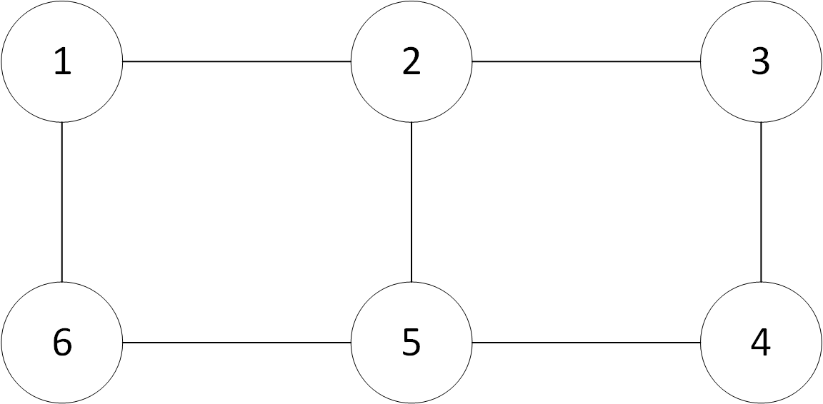
Figure 1: The communication graph.

The initial values $x_{i}(0)=0$. Let (3)-(5) be the updating law with $\alpha_{k}=\frac{10}{k+1}$ and $\tau_{k}=10(k+1)^{0.4}$.

Let $\xi$ be a random variable with $\xi=\omega-2w_{\min}$ where $\omega$ satisfies Pareto distribution with tail index $\gamma=2$ and $\omega_{\min}=1$. The probability density function of $\omega$ can be described as $p(w)=\left\{\begin{array}[]{cc}0,&\text{ if }w\leq w_{\min},\\ \frac{2w_{\min}^{2}}{w^{3}},&\text{ if }w>w_{\min}.\end{array}\right.$ The expectation of $w$ is ${2w_{\min}}$ and the variance is infinity. Thus, $E[\xi]=E[\omega]-2w_{\min}=0$. Moreover, since $p(\xi)=\left\{\begin{array}[]{cc}0,&\text{ if }\xi\leq-w_{\min},\\ \frac{2w_{\min}^{2}}{(\xi+2w_{\min})^{3}},&\text{ if }\xi>-w_{\min},\end{array}\right.$ we have for $\delta=\frac{3}{2}$,

$$E[|\xi|^{\delta}] =\int_{-\infty}^{+\infty}|\xi|^{\delta}p(\xi)d\xi$$

$$=\int_{-w_{\min}}^{+\infty}|\xi|^{\delta}\frac{2w_{\min}^{2}}{(\xi+2w_{\min})^{3}}d\xi$$

$$\leq\int_{-w_{\min}}^{0}|\xi|^{\delta}\frac{2w_{\min}^{2}}{w_{\min}^{3}}d\xi+\int_{0}^{1}\xi^{\delta}\frac{2w_{\min}^{2}}{(2w_{\min})^{3}}d\xi$$

$$+\int_{1}^{\infty}\xi^{\delta}\frac{2w_{\min}^{2}}{\xi^{3}}d\xi$$

$$=\frac{2\omega_{\min}^{\delta}}{(\delta+1)}+\frac{1}{4\omega_{\min}(\delta+1)}+\frac{2w_{\min}^{2}}{2-\delta}$$

$$\approx 4.9<3^{\delta}.$$ (36)

Let $\xi_{i,k}=\omega_{i,k}-2$ where each element of $\omega_{i,k}$ satisfies Pareto distribution with tail index 2 and the minimum parameter 1. Based on the above analysis, $E[\xi_{i,k}]=0$ and $E[\|\xi_{i,k}\|^{\delta}]=E[(\|\xi_{i,k}\|^{2})^{\frac{\delta}{2}}]\leq E[(6\max|{[\xi_{i,k}]_{j}}|^{2})^{\frac{\delta}{2}}]<8^{\delta}$. Thus, $\xi_{i,k}$ satisfies Assumptions 4 and 5.

Fig. 2 shows the evolution of $\sum_{i=1}^{6}\|x_{i,k}-\theta^{*}\|$. As can be seen, the algorithm converges to the optimal solution.

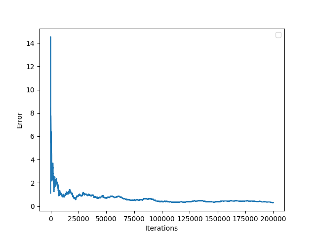
Figure 2: The evolution of $\sum_{i=1}^{6}\|x_{i,k}-\theta^{*}\|$.

Simulation with Different Tail Index: It can be verified that noises with tail index $\gamma>1$ satisfy Assumptions 4 and 5. When $\gamma>2$, the variance is bounded. The evolution of $\sum_{i=1}^{6}\|x_{i,k}-\theta^{*}\|$ with tail index is shown in Fig. 3. It can be seen that a larger tail index can lead to faster convergence.

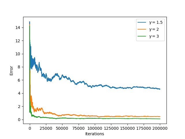
Figure 3: The evolution of $\sum_{i=1}^{6}\|x_{i,k}-\theta^{*}\|$ for $\gamma=1.5$, 2 and 3.

Comparison with [5]: We compare our algorithm with the distributed stochastic subgradient projection algorithm proposed in [5] despite that the Patero random noise does not satisfy the bounded variance condition (Assumption 4 of [5]). When $\mu$ is small, it is found that the performance of our algorithm is similar to that of [5]. Let $\mu=10$. The simulation result is shown in Fig. 4. The performance of our algorithm is better than that of [5].

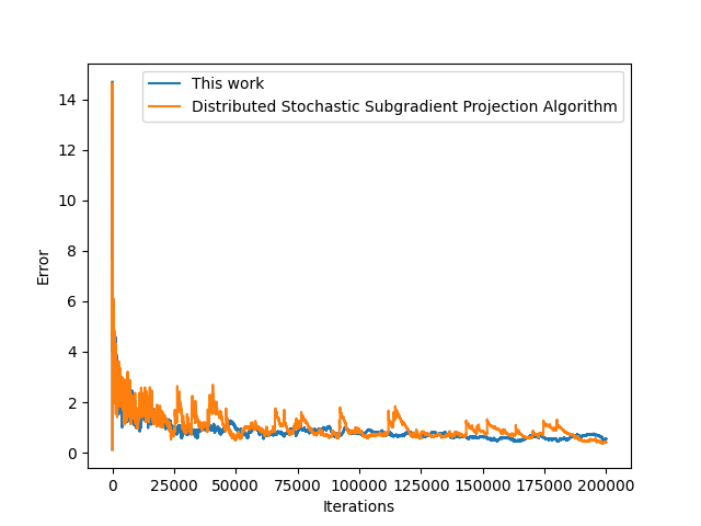
Figure 4: The evolution of $\sum_{i=1}^{6}\|x_{i,k}-\theta^{*}\|$ under our algorithm and the distributed stochastic subgradient projection algorithm proposed in [5].

VI Conclusions

In this paper, we considered the distributed optimization problem under the influence of heavy-tailed noises. Unlike previous studies on heavy-tailed noises, we proposed a distributed update law that only uses neighboring information and the network does not have a central node. Unlike previous studies on distributed stochastic optimization, this paper considers the assumption of heavy-tailed distributions instead of the commonly considered bounded variance noises, which is a broader assumption. The simulation results demonstrate the effectiveness of the algorithm. In future, we will investigate the algorithm design for distributed optimization problems with inequality constraints.

Chao Sun received his B.Eng degree from University of Science and Technology of China in 2013. Then he obtained the Ph.D. degree from School of Electrical and Electronics Engineering, Nanyang Technological University, Singapore in 2018. After graduation, he worked as a research fellow at Nanyang Technological University till May 2022. Currently, he is an associate professor at Beihang University, China.

References

- [1] T. Yang, X. Yi, J. Wu, Y. Yuan, D. Wu, Z. Meng, Y. Hong, H. Wang, Z. Lin, and K. H. Johansson, ``A survey of distributed optimization,'' Annual Reviews in Control, vol. 47, pp. 278–305, 2019.
- [2] K. I. Tsianos, S. Lawlor, and M. G. Rabbat, ``Consensus-based distributed optimization: Practical issues and applications in large-scale machine learning,'' in 2012 50th annual allerton conference on communication, control, and computing (allerton). IEEE, 2012, pp. 1543–1550.
- [3] P. Yi, Y. Hong, and F. Liu, ``Initialization-free distributed algorithms for optimal resource allocation with feasibility constraints and application to economic dispatch of power systems,'' Automatica, vol. 74, pp. 259–269, 2016.
- [4] C. Sun, Z. Feng, and G. Hu, ``Time-varying optimization-based approach for distributed formation of uncertain euler–lagrange systems,'' IEEE Transactions on Cybernetics, vol. 52, no. 7, pp. 5984–5998, 2021.
- [5] S. Sundhar Ram, A. Nedić, and V. V. Veeravalli, ``Distributed stochastic subgradient projection algorithms for convex optimization,'' Journal of optimization theory and applications, vol. 147, pp. 516–545, 2010.
- [6] K. Srivastava and A. Nedic, ``Distributed asynchronous constrained stochastic optimization,'' IEEE journal of selected topics in signal processing, vol. 5, no. 4, pp. 772–790, 2011.
- [7] Z. Wang, J. Zhang, T.-H. Chang, J. Li, and Z.-Q. Luo, ``Distributed stochastic consensus optimization with momentum for nonconvex nonsmooth problems,'' IEEE Transactions on Signal Processing, vol. 69, pp. 4486–4501, 2021.
- [8] K. Lu, H. Wang, H. Zhang, and L. Wang, ``Convergence in high probability of distributed stochastic gradient descent algorithms,'' IEEE Transactions on Automatic Control, 2023.
- [9] J. Zhang, S. P. Karimireddy, A. Veit, S. Kim, S. Reddi, S. Kumar, and S. Sra, ``Why are adaptive methods good for attention models?'' Advances in Neural Information Processing Systems, vol. 33, pp. 15 383–15 393, 2020.
- [10] H. Yang, P. Qiu, and J. Liu, ``Taming fat-tailed (“heavier-tailed” with potentially infinite variance) noise in federated learning,'' Advances in Neural Information Processing Systems, vol. 35, pp. 17 017–17 029, 2022.
- [11] U. Simsekli, L. Sagun, and M. Gurbuzbalaban, ``A tail-index analysis of stochastic gradient noise in deep neural networks,'' in International Conference on Machine Learning. PMLR, 2019, pp. 5827–5837.
- [12] M. Gurbuzbalaban, U. Simsekli, and L. Zhu, ``The heavy-tail phenomenon in sgd,'' in International Conference on Machine Learning. PMLR, 2021, pp. 3964–3975.
- [13] H. Wang, M. Gurbuzbalaban, L. Zhu, U. Simsekli, and M. A. Erdogdu, ``Convergence rates of stochastic gradient descent under infinite noise variance,'' Advances in Neural Information Processing Systems, vol. 34, pp. 18 866–18 877, 2021.
- [14] S. A. Alghunaim and A. H. Sayed, ``Distributed coupled multiagent stochastic optimization,'' IEEE Transactions on Automatic Control, vol. 65, no. 1, pp. 175–190, 2019.
- [15] S. Pu and A. Nedić, ``Distributed stochastic gradient tracking methods,'' Mathematical Programming, vol. 187, pp. 409–457, 2021.
- [16] D. Yuan, Y. Hong, D. W. Ho, and G. Jiang, ``Optimal distributed stochastic mirror descent for strongly convex optimization,'' Automatica, vol. 90, pp. 196–203, 2018.
- [17] E. Gorbunov, M. Danilova, and A. Gasnikov, ``Stochastic optimization with heavy-tailed noise via accelerated gradient clipping,'' Advances in Neural Information Processing Systems, vol. 33, pp. 15 042–15 053, 2020.
- [18] Z. Liu, T. D. Nguyen, T. H. Nguyen, A. Ene, and H. Nguyen, ``High probability convergence of stochastic gradient methods,'' in International Conference on Machine Learning. PMLR, 2023, pp. 21 884–21 914.
- [19] A. Cutkosky and H. Mehta, ``High-probability bounds for non-convex stochastic optimization with heavy tails,'' Advances in Neural Information Processing Systems, vol. 34, pp. 4883–4895, 2021.
- [20] M. Liu, Z. Zhuang, Y. Lei, and C. Liao, ``A communication-efficient distributed gradient clipping algorithm for training deep neural networks,'' Advances in Neural Information Processing Systems, vol. 35, pp. 26 204–26 217, 2022.
- [21] S. Yu, D. Jakovetic, and S. Kar, ``Smoothed gradient clipping and error feedback for distributed optimization under heavy-tailed noise,'' arXiv preprint arXiv:2310.16920, 2023.
- [22] E. Gorbunov, A. Sadiev, M. Danilova, S. Horváth, G. Gidel, P. Dvurechensky, A. Gasnikov, and P. Richtárik, ``High-probability convergence for composite and distributed stochastic minimization and variational inequalities with heavy-tailed noise,'' arXiv preprint arXiv:2310.01860, 2023.
- [23] S. S. Ram, A. Nedic, and V. V. Veeravalli, ``Distributed subgradient projection algorithm for convex optimization,'' in 2009 IEEE International Conference on Acoustics, Speech and Signal Processing. IEEE, 2009, pp. 3653–3656.
- [24] M. O. Sayin, N. D. Vanli, S. S. Kozat, and T. Başar, ``Stochastic subgradient algorithms for strongly convex optimization over distributed networks,'' IEEE Transactions on network science and engineering, vol. 4, no. 4, pp. 248–260, 2017.
- [25] A. Sadiev, M. Danilova, E. Gorbunov, S. Horváth, G. Gidel, P. Dvurechensky, A. Gasnikov, and P. Richtárik, ``High-probability bounds for stochastic optimization and variational inequalities: the case of unbounded variance,'' arXiv preprint arXiv:2302.00999, 2023.
- [26] A. Y. Ng, ``Feature selection, l 1 vs. l 2 regularization, and rotational invariance,'' in Proceedings of the twenty-first international conference on Machine learning. ACM, 2004, p. 78.