Optimized experiment design and analysis for fully randomized benchmarking

Abstract

Randomized benchmarking (RB) is a widely used strategy to assess the quality of available quantum gates in a computational context. RB involves applying known random sequences of gates to an initial state and using a final measurement step to determine ‘success’ or ‘failure’ for each trial. The probabilities of success and failure over many trials can be used to determine an effective depolarizing error per step of the sequence, which is a metric of the gate quality. Here we investigate the advantages of fully randomized benchmarking, where a new random sequence is drawn for each experimental trial. The advantages of full randomization include smaller confidence intervals on the inferred step error, the ability to use maximum likelihood analysis without heuristics, straightforward optimization of the sequence lengths, and the ability to model and measure behaviors that go beyond the typical assumption of time-independent error rates. We discuss models of time-dependent or non-Markovian errors that generalize the basic RB model of a single exponential decay of the success probability. For any of these models, we implement a concrete protocol to minimize the uncertainty of the estimated parameters with a fixed constraint on the time for the complete experiment, and we implement a maximum likelihood analysis. Furthermore, we consider several previously published experiments and determine the potential for improvements with optimized full randomization. We experimentally observe such improvements in Clifford randomized benchmarking experiments on a single trapped ion qubit at the National Institute of Standards and Technology (NIST). For an experiment with uniform lengths and intentionally repeated sequences the step error was $2.42^{+0.30}_{-0.22}\times 10^{-5}$, and for an optimized fully randomized experiment of the same total duration the step error was $2.57^{+0.07}_{-0.06}\times 10^{-5}$. We find a substantial decrease in the uncertainty of the step error as a result of optimized fully randomized benchmarking.

1 Introduction

Benchmarking quantum gates is an important task for the design, development, and characterization of a quantum processor [1]. Randomized benchmarking is a widely-used method to benchmark gates in a computational context that takes advantage of long sequences of gates to efficiently gain statistical information even when large errors in state preparation and measurement (SPAM) are present [2, 3, 4, 5, 6, 7, 8, 9, 10, 11, 12, 13]. In general, a randomized benchmarking trial consists of state preparation, followed by a random sequence of steps drawn from a carefully chosen distribution, followed by a measurement indicating ‘success’ or ‘failure’ for the trial depending on whether or not the nominal outcome is observed. The simplest example is standard randomized benchmarking, where each step is drawn from a two-design [14, 11]. If each step is modeled as a perfect unitary gate followed by an error channel, and if that error channel is independent of time, sequence position, and the gate that is applied, then the probability of the ‘success’ outcome decays exponentially as a function of sequence length [12]. The rate of this exponential decay is interpreted as the average fidelity of a step in a computational context. In addition to standard randomized benchmarking, a wide variety of other randomized benchmarking variants have been proposed and studied in recent years. For example, some variants are designed to characterize the fidelity of gates that aren’t compatible with two-designs [15], and other variants are designed for inference of system parameters other than the average fidelity of steps [16, 17]. In many such situations the behavior of the success probability as a function of sequence length can deviate from a single exponential decay [18, 19, 15, 20].

Due to hardware limitations, current experimental implementations of all variants of randomized benchmarking intentionally repeat each random sequence many times to collect statistics about the probability of error. Here we study fully randomized benchmarking, where a new random sequence is drawn for each experimental trial. Any randomized benchmarking variant can be made fully randomized, and in fact most theoretical treatments of randomized benchmarking implicitly or explicitly assume that the experiment is fully randomized. When we compare fully randomized benchmarking to randomized benchmarking with intentionally repeated sequences, we find several concrete advantages of fully randomized benchmarking. Broadly, these advantages come from the fact that, for an arbitrary error channel, a fully randomized benchmarking experiment is statistically indistinguishable from one where the error channel is a depolarizing channel with the same fidelity. The same is not true if sequences are intentionally repeated. In this case, the true error channel determines the distribution of success probabilities over the possible random sequences, and properties of this distribution are observable in the statistics of repeated sequences.

A more detailed summary of the advantages of fully randomized benchmarking is as follows. First, a randomized benchmarking experiment that repeats random sequences will generally have a larger uncertainty in the step error when compared to the same experiment where the sequences are fully randomized. The larger uncertainty comes from increased variance in the estimate of success probability at each sequence length due to the distribution of fidelities over all possible random sequences. This has been studied in Ref. [21] where the authors recommend designing experiments with relatively short sequence lengths in order to mitigate the effect of repeating random sequences. They also argue that the effect from not fully randomizing is small for Pauli error channels, but point out that their arguments do not apply to unitary error channels. In fact, we analyze previously published randomized benchmarking experiments and find evidence in some cases that a significantly smaller uncertainty could have been obtained if the experiment were fully randomized. A second advantage of fully randomized benchmarking is that the choice of the set of sequence lengths and the choice of the number of trials for each sequence length can be optimized in a straightforward way to maximize the information gained during the experiment. In experiments that do not fully randomize, optimization of the experiment design requires knowledge of least-squares weights that are generally unknown and depend on the true error model. Previous work about optimization strategies for randomized benchmarking can be found in Refs. [22, 23, 24]. Ref. [22] provides a heuristic optimization strategy for the basic exponential decay model of randomized benchmarking and suggests choosing a short sequence length and a long sequence length at half the inverse step error. Ref. [23] addresses optimization for a Bayesian inference procedure, and Ref. [24] discusses optimization strategies for non-fully-randomized benchmarking where a particular variance model is chosen. A third advantage of fully randomized benchmarking is that the step error can be inferred by using maximum likelihood in a straightforward way. In contrast, in experiments that intentionally repeat sequences the step error is typically inferred by means of a weighted-least-squares fit with weights that are a priori unknown, which complicates the interpretation of confidence intervals. Finally, fully randomized benchmarking allows for a straightforward analysis of the simplest time-dependent or sequence-position-dependent errors. In fully randomized benchmarking, the only effect of these errors, or of any non-Markovian errors, is to modify the behavior of the success probability as a function of sequence length. We introduce a nested sequence of statistical models for fully randomized benchmarking that can be used to detect this modifed behavior in a straightforward way. Furthermore, the reduced uncertainty of an optimized fully randomized experiment allows for the detection of modified behavior with increased statistical significance.

This paper is organized as follows. In Section 2 we provide an overview of randomized benchmarking, including our conventions for depolarizing channels and step errors. In Section 3 we describe the numerical procedure that we use to optimize the design of an experiment to minimize the uncertainty in the step error according to a pre-chosen statistical model and reference point. In Appendix A we explain how this optimization is equivalent to a maximization of Fisher information. In Section 4 we address other statistical models of fully randomized benchmarking that allow for time-dependent, sequence-position-dependent, or other non-Markovian errors leading to non-exponential decay of the success probability. In Section 5 we make comparisons between previously published randomized benchmarking experiments and optimized fully randomized benchmarking experiments and demonstrate that improvements in uncertainty are possible. In Section 6 we analyze the improvement in uncertainty from fully randomized benchmarking in terms of the underlying distribution of success probabilities over random sequences at a fixed sequence length. We give evidence that the improvement in uncertainty can be significant when the underlying errors are unitary. In Section 7 we describe the statistical analysis we use to infer the step error, which consists of maximum likelihood inference and statistical bootstrapping to obtain confidence intervals. We also describe an empirical likelihood ratio test that we use to possibly reject the basic model of a single exponential decay and demonstrate it on simulated data. In Section 8 we report the results of randomized benchmarking experiments run on a single trapped ion qubit at NIST. We implement fully randomized benchmarking and perform a comparison between randomized benchmarking with uniformly chosen sequence lengths and repeated sequences, fully randomized benchmarking with uniformly chosen sequence lengths, and optimized fully randomized benchmarking, under otherwise equal conditions. We find that substantial reductions in uncertainty are possible.

2 Overview of randomized benchmarking

We describe our conventions and notation for a statistical description of fully randomized benchmarking experiments, with a focus on the basic model of a single exponential decay. For further information and discussion of randomized benchmarking in general, we refer to Refs. [12, 3, 11, 5]. A fully randomized benchmarking experiment consists of many independent trials, where a trial of sequence length $n$ is composed of a state preparation, followed by a random sequence of $n$ steps, followed by measurement indicating ‘success’ or ‘failure’. The content and distribution of the random steps depends on the benchmarking variant in use. For example, in standard randomized benchmarking each step nominally implements a random Clifford gate. The design of a fully randomized experiment consists of the list $\left(n_{j}\right)_{j=1}^{j_{\text{max}}}$ of sequence lengths to be used, and the list $\left(w_{j}\right)_{j=1}^{j_{\text{max}}}$ of the numbers of independently-randomized trials to be performed at each sequence length. In a fully randomized experiment, the order in which the total $\sum_{j}w_{j}$ trials are performed should also be randomized. As we discuss at the end of this section, this can help to minimize the effect of potential time-dependent errors. After the experiment is performed, the data consists of a list $\left(c_{j}\right)_{j=1}^{j_{\text{max}}}$ where $c_{j}$ is number of success counts observed out of $w_{j}$ total trials at the sequence length $n_{j}$. In general, a statistical model for fully randomized benchmarking consists of a list of parameters $\left(\theta_{i}\right)$, which we refer to as $\bm{\theta}$, and a function $P_{\bm{\theta}}(n)$ that determines the success probabilities at each sequence length $n$ in terms of the parameters. The success counts $\left(c_{j}\right)$ are then binomially distributed for each $j$ with success probability $P_{\bm{\theta}}(n_{j})$. We note that the procedures for experiment design and analysis that we describe in Sections 3 and 7 hold for a general model $P_{\bm{\theta}}(n)$. For the purposes of this paper we assume that fully randomized benchmarking on any particular experimental system admits an accurate description in terms of some $P_{\bm{\theta}}(n)$ and corresponding statistical parameters $\bm{\theta}$.

The most common statistical model for randomized benchmarking is a single exponential decay with a rate that represents the step error and a proportionality constant that represents the state preparation and measurement error. We refer to this model as the basic model and provide a concrete definition in Eq. 2.3. The basic model and other models that we consider in Section 4 can be justified under certain assumptions about the behavior of the experimental system in question. For simplicity and completeness, we provide one such set of assumptions.

(i)  Each trial consists of state preparation of a nominal computational basis state $\outerproduct{\psi_{\text{in}}}{\psi_{\text{in}}}$ followed by a random sequence of steps from a two-design [14, 25], followed by a randomized final step that returns the state to a random computational basis state, followed by measurement in the computational basis. For discussion of randomized final steps and measurements see Ref. [11]. In short, randomizing the final step and measurement allows the combined effect of state preparation and measurement errors to be treated as a single depolarizing error channel.

(ii)  In every trial the $k$th step has an error channel $\Lambda_{k}$ that does not depend on the gate that the step nominally implements. The assumption that errors can be modeled by a channel $\Lambda_{k}$ is the Markovian assumption, according to the definition in Ref. [26]. The assumption of gate-independent errors is discussed in further detail in Ref. [6].

(iii)  The system is completely reset after each trial and no memory effects are present between trials. This assumption disallows, for example, the possibility of step errors that depend on the temperature of a trapped ion motional mode [27] that heats over time. However, this assumption still allows for the possibility that step errors can be drawn from a distribution independently for each trial, or can increase throughout a sequence.

When these assumptions are made, the error channels $\Lambda_{k}$ are ‘twirled’ by the random gates from a two-design and become effective depolarizing channels [11]. In general, the parameters of these depolarizing channels can randomly fluctuate trial-to-trial or can depend on the gate index $k$. The success probability of a sequence of length $n$ is determined by the composition of all the depolarizing channels at gate indices less than $n$, which can lead to more complicated behavior than a single exponential decay. To justify the single exponential decay in the basic model, we add a final assumption.

(iv)  The error channels $\Lambda_{k}$ are independent of time and independent of the step index $k$. This assumption ensures that each effective depolarizing channel has the same depolarizing parameter.

Although these assumptions may seem restrictive, a single exponential decay can still be a good model in many situations where gate-dependent or certain time-dependent errors are present [6, 28]. In the case of gate-dependent errors, the observed rate of exponential decay may differ from the average fidelity of the gates relative to a fixed basis [7]. The observed exponential decay rate is still indicative of gate performance, however [7]. In the case of errors that depend on a classically fluctuating quantity like temperature, randomizing the order of sequence lengths during the experiment leads to a success probability at each sequence length that is averaged over the fluctuating quantity. To good approximation, this behavior can lead to an effective model where the step errors randomly fluctuate trial-to-trial independently. For further information about error models and assumptions in randomized benchmarking, we refer to Refs. [29, 7, 6, 28].

We now provide notation and conventions for the basic model. We use the standard definition that a depolarizing channel $\Phi$ on a Hilbert space of dimension $D$ with a depolarizing parameter $\lambda$ maps an input state $\rho$ to $\Phi(\rho)=(1-\lambda)\rho+\lambda I/D$ where $I$ is the identity operator on Hilbert space and $\lambda$ satisfies $0\leq\lambda\leq 1+1/(D^{2}-1)$. If a system is initialized in a pure state $\outerproduct{\psi}{\psi}$ and a depolarizing channel with parameter $\lambda$ is applied, the fidelity $f$ of the output state with the input state is

$$f=\text{tr}\left[\Phi(\outerproduct{\psi}{\psi})\cdot\outerproduct{\psi}{\psi}\right]=1-\lambda+\lambda/D.$$ (2.1)

The fidelity $f$ does not depend on the input state $\outerproduct{\psi}{\psi}$, and therefore the average fidelity of the depolarizing channel $\Phi$ is equal to $f$. We refer to $\varepsilon=1-f$ as the error of the depolarizing channel $\Phi$. If depolarizing channels with parameters $\{\lambda_{i}\}$ are concatenated, the resulting channel is a depolarizing channel with parameter $\lambda=1-\prod_{i}(1-\lambda_{i})$. When the fidelity of the concatenated channel is expressed in terms of the individual errors it simplifies to the following

$$f=\frac{1}{D}+\frac{1}{\alpha}\prod_{i}(1-\alpha\varepsilon_{i}),$$ (2.2)

where $\alpha=\frac{D}{D-1}$. This motivates the following definition of the basic model,

$$P_{\bm{\theta}}(n)=\frac{1}{D}+\frac{1}{\alpha}(1-\alpha\theta_{0})(1-\alpha\theta_{1})^{n},$$ (2.3)

where $n$ is the sequence length, $\theta_{0}$ is the SPAM error, and $\theta_{1}$ is the step error. Here $n$ is a non-negative integer, and $\theta_{0},\theta_{1}\in[0,1]$. In Section 4 we describe several other models of experimental interest that generalize the basic model. An important property of the basic model is that the SPAM parameter $\theta_{0}$ appears affine linearly in the expression for $P_{\bm{\theta}}(n)$. As a result, a randomly fluctuating SPAM parameter is indistinguishable from a constant SPAM parameter equal to the mean of the distribution of random fluctuations. Fully randomized benchmarking is therefore insensitive to drifts in the SPAM parameter, as long as the drifts are uncorrelated with the choice of sequence lengths. The possibility of drifting SPAM errors was a concern, for example, in Ref. [30] where it affected the design of the randomized benchmarking experiment.

3 Optimized experiment design for fully randomized benchmarking

We describe a procedure to optimize the design of a fully randomized benchmarking experiment for statistical performance according to an arbitrary pre-chosen statistical model $P_{\bm{\theta}}(n)$. The goal of the optimization is to minimize the anticipated uncertainty of the inference of the parameter of interest, $\theta_{i_{0}}$. In many cases the parameter of interest is the step error $\theta_{1}$. The optimization is performed by linearizing the model around a reference point $\bm{\theta}^{(0)}$ and constructing a linear estimator for $\theta_{i_{0}}$ that has minimum variance and is insensitive to the other parameters at the reference point. The standard deviation of the optimal linear estimator is the uncertainty of inference of $\theta_{i_{0}}$ in the linearized model, and is therefore a ‘first-order’ approximation of the anticipated uncertainty of inference of $\theta_{i_{0}}$ in the actual model. The accuracy of this approximation depends on the ‘closeness’ of the reference point to the true point and on the nearby ‘curvature’ of the statistical model. For more details we refer to Refs. [31, 32]. We assume that the models of fully randomized benchmarking considered here are reasonably well-behaved and that a sufficiently accurate reference point can be obtained from prior calibration.

The optimized experiment design that we describe here is called C-optimal design, and it can be formulated as a linear program [33, 34]. Other types of optimization with different objectives are also possible. For example, a general formulation of C-optimal design minimizes the variance of an arbitrary linear combination of model parameters. Similarly, another objective could be to jointly minimize a weighted sum of variances of several parameters. All of these objectives lead to convex optimization problems and have a close connection to Fisher information [31, 33, 32]. For convenience, in Appendix A we provide a description of the relationship between C-optimal design and Fisher information. For more information and details about these types of optimized experiment design, we refer to Refs. [35, 31, 36, 33].

Here we present the optimization procedure to minimize the anticipated uncertainty of a single parameter $\theta_{i_{0}}$, specifically in the context of designing experiments for fully randomized benchmarking. The optimization is performed over the parameters $n_{j}$ and $w_{j}$ of the experimental design, subject to a constraint on the total experimental time $T$. Altogether, the inputs to the optimization are: the statistical model $P_{\bm{\theta}}(n)$, the reference point $\bm{\theta}^{(0)}$, the pre-chosen parameter $\theta_{i_{0}}$, the maximum sequence length $n_{\text{max}}$ that is available in an experiment, and a list $t_{n}$ of the amount of experiment time that it takes to experimentally perform a sequence of length $n$. The details of the optimization procedure are as follows. Let $P_{\bm{\theta}^{(0)}}(n)$ denote the success probabilities at the reference point $\bm{\theta}^{(0)}$ as a function of the sequence length $n$, and let $\delta p_{n}$ denote small changes in $P_{\bm{\theta}}(n)$ around $P_{\bm{\theta}^{(0)}}(n)$, so $P_{\bm{\theta}}(n)=P_{\bm{\theta}^{(0)}}(n)+\delta p_{n}$. Any differentiable model can be linearized around the reference point $P_{\bm{\theta}^{(0)}}(n)$. Let $L_{ni}=\frac{\partial P(n)}{\partial\theta_{i}}\rvert_{\bm{\theta}^{(0)}}$ be the gradient of the model at the reference point. Then we can write

$$\delta p_{n}=\sum_{i}L_{ni}\delta\theta_{i},$$ (3.1)

to first order in the $\delta\theta_{i}$. For the purpose of optimization we now assume the linearized model.

Let $\delta\hat{p}_{n}$ denote the empirical estimator of $\delta p_{n}$ obtained from the observed frequency of successes after subtracting the probability of success at the reference point. If we denote the observed number of success counts by $\hat{c}_{n}$, we have

$$\delta\hat{p}_{n}=\frac{\hat{c}_{n}}{w_{n}}-P_{\bm{\theta}^{(0)}}(n).$$ (3.2)

We consider linear estimators $\hat{A}$ of the form

$$\hat{A}=\sum_{n}C_{n}\delta\hat{p}_{n},$$ (3.3)

where we choose the coefficients $C_{n}$ so that $\hat{A}$ estimates $\delta\theta_{i_{0}}$ with minimum variance at the reference point. Concretely, $\hat{A}$ estimates $\delta\theta_{i_{0}}$ if the coefficients satisfy $\sum_{n}C_{n}L_{ni}=\delta_{ii_{0}}$, which implies that $\langle\hat{A}\rangle=\delta\theta_{i_{0}}$ and that $\hat{A}$ is insensitive to the other parameters $\theta_{i\neq i_{0}}$. Of the many linear estimators that satisfy these constraints, we wish to construct one with the minimum variance at the reference point, subject to the additional constraint that the experiment takes a total time $T$. If a trial with a sequence of length $n$ takes a time $t_{n}$, then this constraint can be expressed as $\sum_{n}w_{n}t_{n}=T$. At the reference point the variance $v_{n}$ of $\delta\hat{p}_{n}$ is determined by the number of trials $w_{n}$ and the binomial statistics of a single trial according to

$$v_{n}=\text{var}\,\delta\hat{p}_{n}=\frac{P_{\bm{\theta}^{(0)}}(n)\pqty{1-P_{\bm{\theta}^{(0)}}(n)}}{w_{n}}.$$ (3.4)

It follows that the variance $V$ of $\hat{A}$ satisfies

$$V=\text{var}\,\hat{A}=\sum_{n}C_{n}^{2}\frac{v_{n}}{w_{n}},$$ (3.5)

where we have used the independence of $\delta\hat{p}_{n}$ for different $n$. In total, to construct the optimal linear estimator we minimize $V$ jointly over the $C_{n}$ and the $w_{n}$, subject to the constraints $\sum_{n}C_{n}L_{ni}=\delta_{ii_{0}}$ and $\sum_{n}w_{n}t_{n}=T$. We are free to optimize over the $C_{n}$ and the $w_{n}$ in either order. The optimization of the $w_{n}$ at fixed $C_{n}$ yields a closed form solution, which can then be optimized over choices of the $C_{n}$ by a linear program as explained in the following paragraph.

We now fix the $C_{n}$ and minimize $V$ over choices of the $w_{n}$ subject to the constraint $\sum_{n}w_{n}t_{n}=T$. For this we introduce the Lagrange multiplier $\lambda$ and find the critical points with respect to $w_{n}$ of

$$V_{\lambda}=\sum_{n}C_{n}^{2}\frac{v_{n}}{w_{n}}+\lambda\left(\sum_{n}w_{n}t_{n}-T\right).$$ (3.6)

Differentiating by $w_{n}$ and solving for $w_{n}$ gives the critical point equations

$$w_{n}=\frac{\absolutevalue{C_{n}}\sqrt{v_{n}}}{\sqrt{\lambda}\sqrt{t_{n}}},$$ (3.7)

which we substitute back into the expression for $V_{\lambda}$ to obtain

$$V_{\lambda,\text{opt}} =\sum_{n}|C_{n}|\sqrt{\lambda}\sqrt{v_{n}t_{n}}+\lambda\left(\sum_{n}\frac{|C_{n}|\sqrt{v_{n}t_{n}}}{\sqrt{\lambda}}-{T}\right)$$

$$=2\sqrt{\lambda}\sum_{n}|C_{n}|\sqrt{v_{n}t_{n}}-\lambda T.$$ (3.8)

Substituting the solution for $w_{n}$ into the constraint and rearranging terms constrains $\lambda$ according to ${\lambda}=\left({\sum_{n}\absolutevalue{C_{n}}\sqrt{v_{n}t_{n}}}/{T}\right)^{2}$. Substituting this value for $\lambda$ into the expression for $V_{\lambda,\text{opt}}$ gives the minimum variance for fixed $C_{n}$

$$V_{\text{opt}} =\frac{1}{T}\left(\sum_{n}\absolutevalue{C_{n}}\sqrt{v_{n}t_{n}}\right)^{2}.$$ (3.9)

To minimize $V_{\text{opt}}$ over the constrained values of $C_{n}$, it suffices to minimize the quantity $F=\sum_{n}\absolutevalue{C_{n}}\sqrt{v_{n}t_{n}}$ with the linear constraints $\sum_{n}C_{n}L_{ni}=\delta_{ii_{0}}$. This can be done by means of a linear program using a standard method for handling the absolute values [37]. The resulting linear program is

Minimize: $$F=\sum_{n}\tilde{C}_{n}\sqrt{v_{n}t_{n}}$$

Variables: $$\left(C_{n}\right)_{n=1}^{n_{\text{max}}},\left(\tilde{C}_{n}\right)_{n=1}^{n_{\text{max}}}$$

Subject to: $$\textrm{for all $n$,}\tilde{C}_{n}\geq 0,$$

$$\textrm{for all $n$},-\tilde{C}_{n}\leq C_{n}\leq\tilde{C}_{n},$$

$$\sum_{n}C_{n}L_{ni}=\delta_{ii_{0}}.$$ (3.10)

Once the optimal $C_{n}$ are determined, the optimal $w_{n}$ can be determined by substitution into Eq. 3.7. After this substitution the optimal $w_{n}$ will be non-negative real numbers, and must be rounded to integer values to design a real experiment. In practice the rounding has only a small effect on the statistical power of the experiment. In total, this optimization method determines the experiment design that has the minimum variance of the best linear estimator of the parameter $\bm{\theta}^{(0)}$ in the linearized model at the reference point. This variance can be computed in terms of the optimal $C_{n}$ according to Eq. 3.9. As we describe in Section 7, for analysis of randomized benchmarking data we use the maximum likelihood-estimator in the full model. In the limit of a large amount of collected data we expect the variance of the maximum likelihood-estimator in the full model to match the variance of the best linear estimator of $\bm{\theta}^{(0)}$ in the linearized model. In any realistic scenario discrepancies can arise between the two variances as a result of the finite amount of collected data, or because the reference point used for the optimization differs from the true point. In this sense, the anticipated variance of the optimal experiment design in Eq. 3.9 should be regarded as approximate, although we expect good agreement in well-behaved cases. For example, in the randomized benchmarking experiments run at NIST that we describe in Section 8, we find that the anticipated variance closely matches the observed variance.

4 Models of Randomized Benchmarking

Here we consider several models of fully randomized benchmarking that generalize the basic model. First, we consider a model where the step error is constant throughout the random sequence of an individual trial, but is drawn from a probability distribution $\tilde{\sigma}(\varepsilon)$ independently for each trial. Accordingly, the success probability $P(n)$ is

$$P(n)=\frac{1}{D}+\frac{1}{\alpha}(1-\alpha\theta_{0})\int d\varepsilon\tilde{\sigma}(\varepsilon)(1-\alpha\varepsilon)^{n},$$ (4.1)

where $\alpha=\frac{D}{D-1}$ and the parameter $\theta_{0}$ describes the SPAM error. As written, this model is parametrized by $\theta_{0}$ and $\tilde{\sigma}$, which is an infinite dimensional parameter. Below we show that only $N+1$ parameters are relevant if the sequence length is bounded by $N$. The basic model corresponds to the case of $\tilde{\sigma}(\epsilon)=\delta(\epsilon-\theta_{1})$, where $\theta_{1}$ is the step error and $\delta$ denotes the Dirac delta distribution. For a general distribution $\tilde{\sigma}(\varepsilon)$, we denote the mean of $\tilde{\sigma}(\varepsilon)$ by $\theta_{1}$ and interpret it as the parameter analogous to step error. At times it is convenient to shift the probability distribution $\tilde{\sigma}(\varepsilon)$ by its mean $\theta_{1}$. We define $\sigma(\varepsilon)=\tilde{\sigma}(\varepsilon+\theta_{1})$ so that

$$P(n)=\frac{1}{D}+\frac{1}{\alpha}(1-\alpha\theta_{0})\int d\varepsilon\sigma(\varepsilon)(1-\alpha\theta_{1}-\alpha\varepsilon)^{n}.$$ (4.2)

The parameters of the model are now $\theta_{0},\theta_{1}$, and $\sigma$,where the probability distribution $\sigma$ is constrained to have mean $0$ and support in $[-\theta_{1},1-\theta_{1}]$. The basic model is recovered with $\sigma(\varepsilon)=\delta(\varepsilon)$. Applying the binomial expansion to the $n$’th power in the expression for $P(n)$ gives

$$P(n)=\frac{1}{D}+\frac{1}{\alpha}(1-\alpha\theta_{0})\pqty{(1-\alpha\theta_{1})^{n}+\sum_{k=2}^{n}\binom{n}{k}(1-\alpha\theta_{1})^{n-k}(-\alpha)^{k}\int d\varepsilon\sigma(\varepsilon)\varepsilon^{k}},$$ (4.3)

where the $k=1$ term vanishes by the assumption that $\sigma(\varepsilon)$ has mean $0$. This motivates the introduction of the moment parameters $\theta_{k}:=\int d\varepsilon\sigma(\varepsilon)\varepsilon^{k}$ for $k=2$ to $N$. In terms of these parameters the success probability can be written

$$P(n)=\frac{1}{D}+\frac{1}{\alpha}(1-\alpha\theta_{0})\pqty{(1-\alpha\theta_{1})^{n}+\sum_{k=2}^{n}\binom{n}{k}(1-\alpha\theta_{1})^{n-k}(-\alpha)^{k}\theta_{k}}.$$ (4.4)

We refer to this model as the ‘moments model’ and we refer to the parameters $\theta_{k}$ for $k\geq 2$ as the moments parameters. For practical use, the moments parameters are truncated for $k$ larger than some $k_{\text{max}}$, so that $\theta_{k}=0$ for $k>k_{\text{max}}$. For example, when we make certain comparisons to published experiments in Section 5, we use the moments model with two non-zero moments parameters $\theta_{2},\theta_{3}$ for a total of four parameters. When we design the experiments in Section 8 we also use the moments model with four total parameters. When we analyze those experiments we use the moments model with three total parameters, where we remove $\theta_{3}$. In that case, we report $\sqrt{\theta_{2}}$ because this is on the same scale as $\theta_{1}$ and is the standard deviation of $\sigma$ if $\theta_{2}$ comes from a true probability distribution. We note that if all the moments parameters are zero, the moments model reduces to the basic model with spam error $\theta_{0}$ and step error $\theta_{1}$. We note that the parameters $\theta_{2},\ldots$ are the mean-subtracted moments of the original distribution $\tilde{\sigma}$. For later use, we denote the moments of $\tilde{\sigma}$ as $\tilde{\theta}_{k}=\int d\varepsilon\varepsilon^{k}\tilde{\sigma}(\varepsilon)$. Treating $\theta_{1}$ as a constant, for $k\geq 2$, $\theta_{k}$ is an affine linear combination of $\tilde{\theta}_{2},\ldots\tilde{\theta}_{k}$, and similarly for $\tilde{\theta}_{k}$ in terms of the $\theta_{2},\ldots,\theta_{k}$.

The moments model is universal in the following sense. In the absence of trial-dependent step errors, the most general benchmarking model has arbitrary success probabilities $P(n)$ depending on $n$. We show that any such success probabilities can be modeled by a suitable choice of parameters of the moments model, provided the implicit linear restrictions on the moment parameters due to positivity and support constraints of the probability distribution $\sigma$ are lifted. We first write the moments model in terms of the moments of $\tilde{\sigma}$,

$$P(n)=\frac{1}{D}+\frac{1}{\alpha}(1-\alpha\theta_{0})\pqty{1+\sum_{k=1}^{n}\binom{n}{k}(-\alpha)^{k}\tilde{\theta}_{k}}.$$ (4.5)

The parameter $\theta_{0}$ linearly determines and is determined by $P(0)$. For the remaining probabilities, we fix $\theta_{0}$. Eq. 4.5 establishes a linear relationship between the $P^{\prime}(n)=P(n)-P(0)$ for $n\geq 1$ and the $\tilde{\theta}_{k}$ for $k\geq 1$ of the form $P^{\prime}(n)=\sum_{k\geq 1}M_{nk}\tilde{\theta}_{k}$. The matrix $M_{nk}$ is lower triangular with diagonal entries $M_{nn}=(P(0)-1/D)(-\alpha)^{n}$. Here we assume that $P(0)\neq 1/D$. If $P(0)=1/D$, then the initial state would be completely depolarized and the choice of moment parameters would be irrelevant. With this assumption the diagonal entries $M_{nn}$ are nonzero, and $M$ therefore has a lower triangular inverse. It follows that in the absence of constraints on the $\tilde{\theta}_{k}$, all possible $P(n)$ can be modeled with a choice of the moment parameters. If the maximum sequence length under consideration is $n_{\text{max}}$, we can truncate the matrix at $n=n_{\text{max}}$ and model $P(0),\ldots P(N)$ with a choice of $\tilde{\theta}_{1},\ldots\tilde{\theta}_{N}$, or equivalently $\theta_{1},\ldots,\theta_{N}$, for any fixed $\theta_{0}$.

In addition to the basic model and the moments model, another model of experimental interest is one where the errors in a sequence experience drift as a function of position within the sequence. To motivate this behavior we consider a miscalibrated single-qubit gate where the miscalibration drifts linearly as a function of time but is reset at the beginning of each sequence. Concretely, we consider a gate $U$ that nominally implements a $\pi$ rotation about the $x$-axis of the Bloch sphere and can be expressed as $U=\exp\left[-i(\pi/2)X\right]$, where $X$ is the Pauli-$X$ operator. We denote the action of the possibly miscalibrated gate by $\tilde{U}=\exp\left[-i(\pi/2+\phi)X\right]$, where $\phi$ is an error parameter that describes the angle of erroneous rotation. The average fidelity of $\tilde{U}$ with the nominal gate $U$ is equal to $1/3+2\cos^{2}(\phi)/3$. A plausible error model is that the erroneous rotation $\phi$ depends linearly on time, which could correspond physically to a linear drift of Rabi frequency. If the gate is perfectly calibrated at $t=0$, expanding to lowest order for short times shows that the error will grow quadratically. If $\phi\neq 0$ at $t=0$ and the expansion is performed to second order, the error will in general have both linear and quadratic dependence for short times. Altogether, this motivates consideration of the following approximate model,

$$P(n)=\frac{1}{D}+\frac{1}{\alpha}(1-\alpha\theta_{0})\pqty{\prod_{k=1}^{n}(1-\alpha(A+Bk+Ck^{2}))},$$ (4.6)

where $\theta_{0}$ is a SPAM parameter and $A,B,C$ are parameters that govern the linear and quadratic drift. One question of possible experimental relevance is whether this drift model can be distinguished from the moments model when the error distribution is restricted to be a true probability distribution $\tilde{\sigma}(\varepsilon)$. Here we show that this is indeed possible for at least one region of the space of parameters. In particular, we consider $\theta_{0}=0,C=0$, and approximate Eq. 4.6 to lowest order in $B$ for $B>0$. When we determine the moments parameters that match this model we find that $\theta_{2}<0$ for this region of parameter space, which is impossible for a true second moment. To determine the matching moments parameters, we follow the procedure outlined in the previous paragraph. In the approximate linear drift model we have $P(1)=1/D+(1-\alpha A-\alpha B)/\alpha$ and in the moments model we have $P(1)=1/D+(1-\alpha\theta_{1})/\alpha$. We equate these to determine $\theta_{1}$ and find $\theta_{1}=A+B$. Similarly, we then equate $P(2)$ in both models

$$(1-\alpha\theta_{1})(1-\alpha\theta_{1}-\alpha B)=(1-\alpha\theta_{1})^{2}+\alpha^{2}\theta_{2}.$$ (4.7)

Solving for $\theta_{2}$ we find $\theta_{2}=-B(1-\alpha\theta_{1})/\alpha$, which satisfies $\theta_{2}<0$ when $B>0$. Equating $P(3)$ in both models we find that $\theta_{3}$ is of order $O(B^{2})$, and by induction we find that $P(k)$ is of order $O(B^{2})$ or higher when $k\geq 3$. We conclude that the parameters $\theta_{k}$ for $k\geq 3$ can be dropped to good approximation when $B$ is small. In total, we conclude that if the true model is the linear drift model for small positive $B$, an analysis using the moments model with parameters $\theta_{0},\theta_{1},\theta_{2}$ would likely find $\theta_{2}<0$ in the large data limit, which is impossible for a true second moment.

5 Analysis of achievable uncertainty improvements

We illustrate the advantages of full randomization by comparing the uncertainties achieved in several published experiments to the uncertainties that could have been achieved with fully randomized benchmarking with the same experiment design. We also demonstrate that additional improvements in uncertainty could have been achieved by optimizing the experiment design according to the procedure in Section 3. The published randomized-benchmarking experiments that we use for specific comparisons are Refs. [38, 9, 8]. For each past experiment we assume that the basic model in Eq. 2.3 is accurate and we use the procedure in Appendix A to construct the optimal linear estimator for step error according to the reported sequence lengths and reported total number of trials at each sequence length, and using the reported step error and SPAM error as the reference point. In all of these experiments the same random sequences were repeated many times, but our construction of the optimal linear estimator assumes that the experiment was fully randomized and that a new random sequence was drawn for each trial. Therefore, we interpret the standard deviation of the optimal linear estimator as the anticipated uncertainty if the experiment had been fully randomized, and we compare it to the uncertainty actually reported by each experiment. Then, we run the optimization described in Section 3 to construct the optimal experiment design according to the basic model. For Refs. [8, 9] we assume that the step time is equal to the SPAM time and for Ref [38] we assume that the step time is $100$ times smaller than the SPAM time. We interpret the anticipated uncertainty returned by the optimization as the size of the confidence interval for each experiment if it had been fully randomized and the optimal experiment design had been used. Finally, we repeat the optimization for the four-parameter moments model to see how the anticipated uncertainty is affected by a more general model. All of these observations are recorded in Table. 1. We generally observe that improvements in uncertainty are possible both from fully randomizing the experiment and from using the optimal experiment design.

Table 1: Results of a numerical signal-to-noise comparison between past randomized benchmarking experiments and experiments optimized according to the procedure in Section 3. The columns show the referenced benchmarking experiment; the gate error and uncertainty reported by each experiment; the anticipated uncertainty for a fully randomized experiment with the reported experiment design; obtained as in Appendix A; and the expected uncertainty if the experiment design is optimized, as described in Section 3, for the basic model and the four-parameter moments model respectively.

Experiment	Reported
step error	Reported
uncertainty	Fully randomized
anticipated
uncertainty
(basic model)	Optimized
anticipated
uncertainty
(basic model)	Optimized
anticipated
uncertainty
(moments model)
Ref. [38]	$2.0\times 10^{-5}$	$2\times 10^{-6}$	$2.1\times 10^{-6}$	$1.0\times 10^{-6}$	$1.6\times 10^{-6}$
Ref. [9]	$8.3\times 10^{-3}$	$2\times 10^{-4}$	$1.2\times 10^{-4}$	$1.1\times 10^{-4}$	$1.7\times 10^{-4}$
Ref. [8]	$5.3\times 10^{-2}$	$4\times 10^{-3}$	$8.8\times 10^{-4}$	$4.3\times 10^{-4}$	$1.3\times 10^{-3}$

In the case of Ref. [8], we observe more than a factor of four improvement in anticipated uncertainty if the experiment is fully randomized. As we show in Section 6, the size of the improvement in uncertainty from fully randomizing depends on the true error model, and is larger if the true errors are closer to unitary errors. For the parameters reported in Ref. [8] we find that an improvement of this size from fully randomizing is possible if the true errors are unitary. Further details of this comparison are in Section 6.

In addition, we numerically explore the improvement obtained by optimizing the experiment design for hypothetical fully randomized experiments. The comparisons are made between uniform experiment designs where the sequence lengths are chosen uniformly in a fixed range and the same number of trials are performed at each sequence length, and optimized experiment designs constructed according to the method in Section 3. The optimized experiment designs are constrained to take the same total time as the corresponding uniform experiments. To compare uniform experiment designs to optimized designs, we compute the standard deviations of the optimal linear estimator in the linearized model, as described in Section 3 and Appendix A, and take the ratio of these standard deviations. Larger ratios indicate a larger benefit from optimizing and the square of this ratio corresponds to the ratio of experiment times required to achieve the same standard deviation. The results of these comparisons are shown in Fig. 1. In plot (a) we use the basic model with the spam error parameter $\theta_{0}$ set to $10^{-2}$ and step error $\theta_{1}\in\left[10^{-6},10^{-2}\right]$. In plot (b) we use the moments model with four total parameters, where the reference values of the moments parameters are set to zero, $\theta_{0}$ is set to $10^{-2}$, and $\theta_{1}$ ranges over $\left[10^{-6},10^{-2}\right]$. In both plots the uniform experiment design consists of $20$ uniformly spaced sequence lengths in the range $[1,1/\theta_{1}]$. The ratio of the SPAM time to the step time is either set to $1$ or $100$ and both options are shown in the plots. At a step error of $10^{-6}$ and when the ratio of the SPAM time to the step time is $100$, we observe a reduction in standard deviation by a factor of $1.96$ for the basic model and by a factor of $5.9$ for the moments model with four parameters. These improvements correspond to time savings by factors of $3.8$ and $35.2$ respectively.

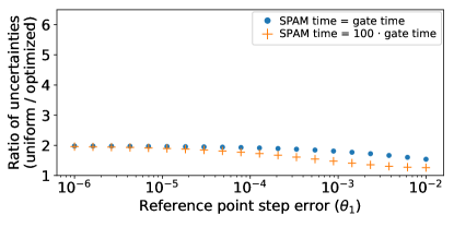
(a)

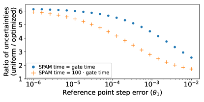
(b)

Figure 1: Comparison between hypothetical fully randomized experiments that use either an optimized experiment design or a uniform design of evenly-weighted sequence lengths. The plots show the ratio of the anticipated standard deviations of the step error (uniform/optimized), as a function of the reference step error. In all cases, the SPAM parameter $\theta_{0}$ is fixed at $10^{-2}$ and the total experiment time set to a constant. For the uniform experiment design, $20$ evenly-spaced sequence lengths from $[1,1/\theta_{1}]$ are used and the number of trials at each length is the same. In both plots, the dots show the comparison assuming that the SPAM time is equal to the step time and the plus signs show the comparison assuming that the SPAM time is larger than the step time by a factor of $100$. Larger ratios indicate a larger benefit from optimizing the experiment design. In plot (a) we use the basic model and in plot (b) we use the moments model with four total parameters.

6 Variance analysis of fully randomized benchmarking

For randomized benchmarking with a fixed set of sequence lengths and a fixed number of trials at each sequence length, fully randomized benchmarking generally yields lower uncertainty than randomized benchmarking with multiple trials for each chosen sequence. The uncertainty reduction depends on the error channels and is due to the sequence-dependent success probabilities for error channels that are not depolarizing. The reduction is particularly pronounced for unitary error channels and may be analyzed by fixing the sequence length $n$ and evaluating the variance of the empirical estimate of $P(n)$ for the general scenario where we run $M=kl$ independent trials consisting of $k$ randomly chosen sequences where each sequence is run $l$ times. For related work on the relationship between the number of random sequences and the variance of a randomized benchmarking experiment, we refer to Refs. [21, 23]. The fully randomized scenario has $k=M$ and $l=1$. We assume a sequence-dependent probability of success $s$. Since the sequence is chosen randomly, the probability of success can be considered as a random variable with probability measure on $s\in[0,1]$ given by $\mu(s)$ that depends on $n$ and the two-design used. The goal is to estimate the average probability of success, which is given by $\bar{s}=\langle s\rangle_{\mu}=\int d\mu(s)s$. For $i=1,\ldots,k$, let $\hat{c}_{i}$ be the number of observed successes for the $i$’th sequence. The minimum variance estimator for $\bar{s}$ is the empirical average $\hat{s}=\frac{1}{k}\sum_{i}\frac{\hat{c}_{i}}{l}$. Because the sequences are independent and identically distributed, each $\hat{c}_{i}$ is identically distributed according to a random variable $C$ which is the sum of $l$ Bernoulli random variables with success probability $S$. The variance of $C$ given $S$ is $lS(1-S)$ and the mean of $C$ given $S$ is $lS$. The variance of $C$ can be computed according to the law of total variance [39] as

$$\text{var}(C) =E(\text{var}(C|S))+\text{var}(E(C|S))$$

$$=l\langle S(1-S)\rangle_{\mu}+l^{2}\langle(S-\bar{s})^{2}\rangle =\;\;\; l\bar{s}(1-\bar{s})+l(l-1)\text{var}(S).\;\;\;$$ (6.1)

This expression appears, for example, in Appendix A of Ref. [23]. The variance of $\hat{s}$ is $\frac{1}{k}\text{var}(C)/l^{2}$. Accordingly,

$$\text{var}\hat{s}=\frac{\bar{s}(1-\bar{s})}{M}+\frac{(l-1)}{M}\pqty{\pqty{\int d\mu(s)s^{2}}-\bar{s}^{2}}.$$ (6.2)

The second term in Eq. 6.2 vanishes if $l=1$, so we can interpret it as the excess variance due to not fully randomizing and we denote it by $Z$. An important point is that $Z$ depends on the exact error model via $\int d\mu(s)s^{2}$. For example, if all errors are depolarizing channels then the success probability is independent of the random sequence and $\int d\mu(s)s^{2}=\bar{s}^{2}$, which implies that $Z=0$. In contrast, if the error channel is a fixed unitary, $S$ depends on the particular sequence and $Z$ may be significant. In this regard the observed variance in success probabilities over random sequences can provide a measure of the amount of coherent error in a randomized benchmarking experiment. This has been observed qualitatively in Ref [3], where the large variance in fidelities at each sequence length is attributed to coherent errors. For related work to distinguish coherent and incoherent errors in a randomized benchmarking experiment by inferring a quantity called the unitarity, we refer to Refs. [17, 40].

To better understand the size of the excess variance $Z$, we consider a specific error model with unitary error channels. Consider an error model where the final state $\psi$ is assumed to be equal to the target state $\chi$ with probability $\lambda$ and is a random pure state with probability $1-\lambda$. To express $\lambda$ in terms of $\bar{s}$, we note that

$$\bar{s}=\lambda+(1-\lambda)\int d\psi_{H}f_{\psi}=\lambda+\frac{1}{D}(1-\lambda),$$ (6.3)

where $d\psi_{H}$ denotes the Haar measure over pure states and $f_{\psi}$ denotes the success probability for each random pure state $\psi$. This relationship can be inverted to solve for $\lambda$ as a function of $\bar{s}$

$$\lambda=\frac{\bar{s}-1/D}{1-1/D}.$$ (6.4)

In order to determine the variance of $\hat{s}$ by substituting into Eq. 6.2 for this error model we first evaluate

$$\int d\mu(s)s^{2}=\lambda+(1-\lambda)\frac{2}{D(D+1)},$$ (6.5)

where we have used the fact that $\int d\psi_{H}f_{\psi}^{2}=\frac{2}{D(D+1)}$ (Appendix C). Substitution for $\lambda$ according to Eq. 6.4 leads to the final expression

$$\text{var}\hat{s}=\frac{\bar{s}(1-\bar{s})}{M}+\frac{l-1}{M}\pqty{\frac{\bar{s}-1/D}{1-1/D}+\frac{1-\bar{s}}{1-1/D}\frac{2}{D(D+1)}-\bar{s}^{2}}.$$ (6.6)

For any given experiment, it is possible to estimate the excess variance due to repetition of sequences by considering the statistics obtained at a particular sequence length. For example, consider a sequence length of $20$ in the experiment reported in Ref. [8]. In this experiment, $D=4$, $k=51$ and $l=125$. At a sequence length of $20$, the reported success probability is $0.31$ and the $95\;\%$ confidence interval has a total size of approximately $0.06$ as determined from Fig. 4a of Ref. [8]. If the experiment had been fully randomized, we would expect a total size of this confidence interval of $0.023$ when analyzed according to the basic model. For comparison, with the unitary error model of the previous paragraph and the parameters reported in Ref. [8], the $95\;\%$ confidence interval would have had a total size of $0.16$. It is therefore possible that the increased size of the reported confidence interval relative to the anticipated confidence interval from fully randomized benchmarking can be explained by coherent errors in the actual experiment.

7 Statistical Analysis

For inference of the model parameters $\bm{\theta}$ for any model $P_{\bm{\theta}}(n)$ we use maximum likelihood whenever it is tractable and well-behaved, which it is for all the examples we consider in this paper. Maximum likelihood has the advantage that it is asymptotically unbiased, meaning that as the amount of collected data grows to infinity, the inferred model parameters match the true point in parameter space. To obtain confidence intervals on one or more parameters one may use statistical bootstrapping, which is a method of resampling the observed data to learn how much the inferred quantities vary as the data varies. For more information about maximum likelihood and statistical bootstrapping we refer to Refs. [41, 42]. Here we provide the log-likelihood function for an arbitrary model and discuss the possibilities for obtaining confidence intervals through statistical bootstrapping. We also discuss a statistical analysis to possibly reject the inner model(s) of a set of nested models using an empirical likelihood ratio test with statistical bootstrapping.

The log-likelihood function for an arbitrary model is as follows. The probability $L_{j}$ of observing $c_{j}$ successes out of $w_{j}$ trials at the sequence length $n_{j}$ is

$$L_{j}=\binom{w_{j}}{c_{j}}(P_{\bm{\theta}}(n_{j}))^{c_{j}}(1-P_{\bm{\theta}}(n_{j}))^{w_{j}-c_{j}}.$$ (7.1)

The total probability is obtained by taking a product over all sequence lengths in the list $\left(n_{j}\right)$. It follows that the full log-probability $\Theta$ is

$$\Theta=\sum_{j=1}^{j_{\text{max}}}\pqty{\log{\binom{w_{j}}{c_{j}}}+c_{j}\log{P_{\bm{\theta}}(n_{j})}+(w_{j}-c_{j})\log{(1-P_{\bm{\theta}}(n_{j}))}}.$$ (7.2)

We note that the dependence on the model parameters $\bm{\theta}$ is entirely through $P_{\bm{\theta}}(n)$.

Parametric or non-parametric bias-corrected bootstrapping [41, 43] can be used to obtain confidence intervals for one or more parameters. In typical uses of bootstrapping in quantum characterization, the bootstrap assumptions are not satisfied, often because the parameters are statistically close to the boundary. As a result, the coverage probabilities do not closely match the nominal confidence levels used. Nevertheless, at moderate confidence levels, the intervals obtained are useful for interpretation but should be treated as approximate. For more information about potential issues with bootstrap coverage probabilities we refer to [44, 45] and for examples and discussion in the context of quantum information science we refer to [46, 47]. When we optimize the design of an experiment according to the procedure in Section 3, the anticipated uncertainty that we minimize is intended to approximate the size of confidence intervals obtained according to the Gaussian assumption, absent any boundary issues. However, for experiments of finite duration the confidence intervals in general do not exactly match the anticipated uncertainty, even if the reference point used for the optimization is equal to the true point. In the limit that the experiment duration and the amount of data become large and a Gaussian model is a good approximation, the confidence interval sizes should match the anticipated uncertainty. There can still be deviations in the large data limit if the reference point used for the optimization does not match the true point.

In some experiments there may be two or more relevant statistical models that are nested, meaning that the inner model can be obtained from the outer model by fixing some of its parameters at constant values. In such a situation, it may be useful to perform a statistical analysis to attempt to reject the inner model. One such method is to use an empirical likelihood ratio test with statistical bootstrapping [42, 2, 48]. A standard likelihood ratio test with a chi-squared analysis would be sufficient if a Gaussian model were accurate. However, in many relevant cases the Gaussian model does not hold and this can lead to noticeable statistical issues [49]. For this reason, one may use an empirical likelihood ratio test which we now describe. We denote the outer model by $P_{\bm{\theta},\bm{\phi}}(n)$, where now there are two sets of statistical parameters $\bm{\theta},\bm{\phi}$. The inner model is obtained by setting $\bm{\phi}$ to some particular value. For a given set of data a maximum likelihood analysis can be run for both models, and the ratio of the maximum likelihood values can be computed. Assuming the inner model is true, the distribution of likelihood ratios can be estimated, empirically, by bootstrap resampling the data according to the inner model and computing the likelihood ratio for each resampled dataset. With this analysis one can reject the inner model at a particular confidence level, which is based on the percentile of the observed likelihood ratio within this empirical distribution of bootstrapped likelihood ratios.

As a concrete example, we conduct a simulated empirical likelihood ratio test to check for deviations from the basic model of fully randomized benchmarking. We consider a model where the SPAM error is fixed at $\theta_{0}=3\times 10^{-2}$ and for each trial the step error $\theta_{1}$ is drawn independently from a Gaussian distribution with mean $1\times 10^{-4}$ and standard deviation $2.5\times 10^{-5}$. To choose an experiment design for the simulated experiment, we use the four-parameter moments model and perform the optimization described in Section 3. For this optimization we choose the reference point to match the moments of the actual Gaussian distribution of the step error, and we minimize the standard deviation of the parameter $\theta_{2}$ as a proxy for maximizing the statistical power to reject the basic model. We choose $\theta_{2}$ as a proxy because $\theta_{3}$ is zero for the chosen distribution of step errors. In the optimized experiment, the standard deviation of the step error $\theta_{1}$ is $1.1\times 10^{-6}$. If the experiment were instead optimized to minimize the standard deviation of $\theta_{1}$, the optimal experiment in that case would have a standard deviation of $8.0\times 10^{-7}$. This illustrates the fact that the decision to optimize the experiment to maximize statistical power to reject the basic model has a relatively small effect on the performance of inferring the step error. The optimized experiment is constrained so that the total run time is $3$ hours, assuming that each step takes $10^{-5}$ s and state preparation and measurement takes $10^{-3}$ s. Once the experiment design has been chosen, we simulate a dataset for this experiment by drawing a step error $\theta_{1}$ independently for each trial. Once a value of $\theta_{1}$ has been drawn, we then draw ‘success’ or ‘failure’ with the corresponding probability obtained from the basic model for the drawn value of $\theta_{1}$ and the particular sequence length in question. With the simulated dataset we then perform a bootstrapped empirical likelihood ratio test between the basic model, three-parameter moments model, and the general model, which are nested models. For each choice of inner model and outer model we follow the procedure outlined in the previous paragraph, and the results are shown in Fig. 2. According to the distribution of bootstrapped likelihood ratios, we can reject the basic model relative to the three-parameter moments model at a p-value of $1.4\%$. No significant deviation from the three-parameter moments model relative to the general model was detected (p-value of 51.0%). These results agree with the intuition that the Gaussian fluctuation in the step error is detectable via the second moment, and that the fourth and higher moments can be safely neglected in this scenario.

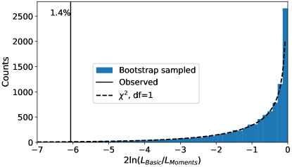
(a) Basic model vs Moments model

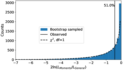
(b) Moments model vs General model

Figure 2: Results of a simulated empirical likelihood ratio test of three nested statistical models of fully randomized benchmarking. The three statistical models that we consider are the basic model, the moments model, and the general model. Further details about these models are in Section 4. The test is conducted using a simulated dataset obtained by drawing the step error $\theta_{1}$ independently for each trial from a Gaussian distribution with mean $1\times 10^{-4}$ and standard deviation $0.25\times 10^{-4}$. To perform the test we use the procedure described in Section 7 in two cases, the first where the inner model is the basic model and the outer model is the three-parameter moments model, and the second where the inner model is the three-parameter moments model and the outer model is the general model. In the first case we can reject basic model with a p-value of $1.4\%$, and in the second case the p-value to reject the three-parameter moments model is $51.0\%$.

8 Experimental Implementation

To provide a concrete comparison between non-fully-randomized benchmarking and optimized fully randomized benchmarking, we designed and implemented three randomized benchmarking experiments. To realize these experiments we perform single qubit rotations on a ²⁵Mg⁺ ion in a microfabricated surface-electrode ion trap, in the apparatus described in Refs. [50, 51]. We use the states $\ket{F=3,m_{F}=1}$ (logical $\ket{1}$) and $\ket{F=2,m_{F}=1}$ (logical $\ket{0}$) in the ${}^{2}S_{1/2}$ ground-state hyperfine manifold to realize a qubit. The qubit transition frequency of $\omega=2\pi\times 1686$ MHz is first-order insensitive to the magnetic field at $B\approx$ 213 G, mitigating against errors caused by fluctuations in the total magnetic field. Qubit rotations around X and Y are implemented with microwave magnetic fields applied at the transition frequency with differing phase, while Z rotations are implemented by adding a phase offset to the microwave control signal for subsequent rotations. The qubit is prepared with optical pumping followed by microwave pulses to transfer population to the $\ket{1}$ state. Qubit readout is accomplished by applying a laser resonant with the ${}^{2}S_{1/2}$ to ${}^{2}P_{3/2}$ cycling transition and detecting state-dependent ion fluorescence as in Ref. [51] (SM). Full randomization is achieved by choosing gates on the fly in real time with a pseudorandom number generator (PRNG) [52] running on the same FPGA (field programmable gate array) that is used to generate the gate pulses applied to the ion. The ideal stabilizer (assuming no errors) is stored and concurrently updated on the FPGA as new gates are chosen, such that when the required number of random gates have been applied the stabilizer can be used to return the qubit to the measurement basis and indicate the expected measurement outcome. The on-the-fly calculation process for sequences can also be configured to enable intentional repetition of random gate sequences.

The three experiments in the comparison are as follows. First, we constructed an experiment where $10$ sequence lengths were set uniformly in the range from $5$ to $1/x_{0}$ where $x_{0}=2\times 10^{-5}$ is the best guess for the step error prior to the experiment. At each sequence length we drew $24$ random sequences and repeated each of them $24$ times. This experiment took roughly $53.5$ minutes of total time. Then, we repeated the same experiment but fully randomized the sequences, so at each sequence length a total of $24\times 24=576$ random sequences were drawn and run once. The time to run the experiment is unaffected by fully randomizing, so this experiment also took $53.5$ minutes of total time. Finally, we designed an optimized, fully randomized experiment using the methods in Section 3. The reference point for the optimization has a SPAM parameter of $3\times 10^{-2}$ and a step error parameter of $2\times 10^{-5}$, and the optimization minimizes the standard deviation of the step error according to the four-parameter moments model. The total time of the optimized experiment was constrained to match the total time of the non-optimized experiments. For experimental simplicity we rounded the number of trials at each sequence length to a multiple of four, so that each experiment could be divided into four equal blocks. Within the first block, the order of experimental trials is randomly chosen and then the same order of trials is repeated for the remaining three blocks. Rounding the number of trials at each sequence length to a multiple of four had a negligible effect on the wall-clock time and anticipated standard deviations.

To analyze the randomized benchmarking experiment with repeated sequences, we ran a weighted least squares fit to the basic model. The weights in the fit are the squared inverses of the empirical standard errors of the success probabilities at each sequence length. The empirical standard errors are obtained by computing the empirical standard deviation of the estimated success probabilities of the random sequences and dividing by the square root of the number of sequence repetitions. For further information about weighted least square fits in randomized benchmarking we refer to Ref. [11]. To analyze the fully randomized experiments we perform the maximum likelihood inference that we outline in Section 7. We perform this maximum likelihood analysis for both the basic model and the moments model with three total parameters. The results for all three experiments are shown in Fig. 3.

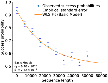
(a) Uniform design, repeated sequences

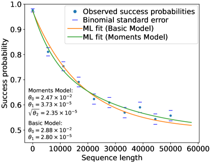
(b) Uniform design, fully randomized

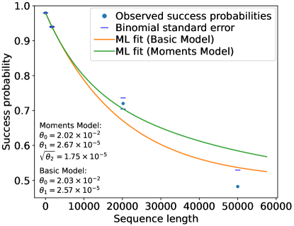
(c) Optimized design, fully randomized

Figure 3: The observed decays in success probability for each of the three randomized benchmarking experiments run at NIST comparing non-fully randomized benchmarking to optimized fully randomized benchmarking. The experiment in plot (a) has sequence lengths chosen uniformly in the range $[5,5\times 10^{4}]$ and for each sequence length $24$ random sequences are drawn and run $24$ times each. The orange trace is the best fit to the basic model, obtained by a weighted least squares fit to the observed success probabilities, and the best fit parameters are shown inset in the lower left. The weights in the fit are the squared inverses of empirical standard errors of the observed success probabilities at each sequence length. These empirical standard errors are shown with the blue tickmarks. The experiment in plot (b) has the same sequence lengths as the first experiment, but is fully randomized so at each sequence length $24\times 24$ random sequences are drawn and run once each. The experiment in plot (c) is designed according to the optimization routine in Section 3, where the total experiment time is constrained to match the total experiment time of each of the previous two experiments. In plots (b,c) the orange and green traces are the maximum likelihood fits to the basic model and the three-parameter moments model respectively, and the maximum likelihood parameters are shown inset in the lower left. The blue ticks show the binomial standard errors of the observed success probabilities.

To obtain confidence intervals on the step error for the various experiments, we perform bias-corrected parametric bootstrapping with $10,000$ bootstrap samples, as described in Section 7 and in Ref. [41]. For the first experiment, which has intentionally repeated sequences, the bootstrap samples are obtained by following the procedure in Ref. [11]. To summarize, first we resample the list of sequences with replacement, and then for each sequence we binomially resample the success and failure counts. Then, for each bootstrapped dataset the step error is estimated with a weighted least squares fit to the model. For the second and third experiments, which are fully randomized, the bootstrap samples are obtained by parametrically resampling according to the parameters obtained from the maximum likelihood analysis on the original data. The bootstrap histograms, point estimates, and $68\%$ bootstrapped confidence intervals are shown in Fig. 4, where we run the analysis according to both the basic model and the three-parameter moments model. For the uniform design with repeated sequences, we report a step error of $2.42^{+0.30}_{-0.22}\times 10^{-5}$ when analyzing according to the basic model. For the optimized fully randomized experiment we report a corresponding step error of $2.57^{+0.07}_{-0.06}\times 10^{-5}$, which has a confidence interval that is roughly four times smaller. To test the basic model of the optimized, fully randomized experiment, we performed the empirical likelihood ratio test described in Section 7. The results are shown in Fig. 5. We found a p-value of $6.0\%$ to reject the basic model. This shows weak evidence of deviation from an exponential decay, which we interpret as evidence of non-Markovian or time-dependent behavior.

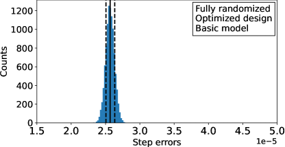
(a)

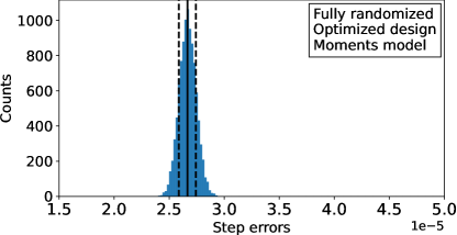
(b)

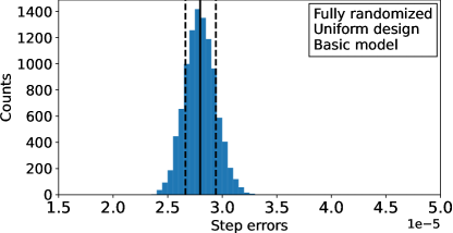
(c)

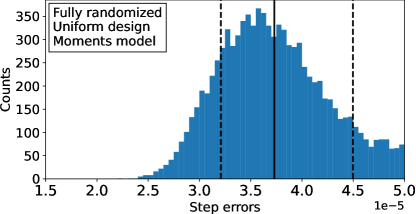
(d)

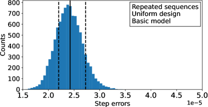
(e)

Figure 4: The bootstrap distributions obtained during the analysis of the three experiments run at NIST during our comparison between non-fully-randomized benchmarking and optimized fully randomized benchmarking. The plots in the left column correspond to the analysis according to the basic model and the plots in the right column correspond to the analysis according to the three-parameter moments model. The plots in the first row are for the optimized, fully randomized experiment, the plots in the second row are for the uniform, fully randomized experiment, and the plot in the third row is for the uniform experiment with repeated sequences. We do not include the plot for the uniform experiment with repeated sequences analyzed according to the moments model because performing a weighted least squares fit to the moments model is not a standard technique in randomized benchmarking. For all the plots, the solid black line indicates the step error parameter of the best fit to the original data and the dashed black lines denote the $68\%$ confidence interval obtained with bias-corrected bootsrapping. The best fit step errors for the plots are (a) $2.57^{+0.07}_{-0.06}\times 10^{-5}$, (b) $2.67^{+0.08}_{-0.08}\times 10^{-5}$, (c) $2.80^{+0.14}_{-0.14}\times 10^{-5}$, (d) $3.73^{+0.77}_{-0.52}\times 10^{-5}$, (e) $2.42^{+0.30}_{-0.22}\times 10^{-5}$.

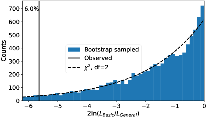
Figure 5: Results of an empirical likelihood ratio test for the optimized, fully randomized experiment. We perform the procedure described in Section 7, with the basic model as the inner model and the general model as the outer model. We find a p-value to reject the basic model of $6.0\%$. This shows weak evidence of deviation from an exponential decay, which we interpret as evidence of non-Markovian or time-dependent behavior.

After completing these three experiments, we intentionally introduced a unitary error by miscalibrating the gates in the 2-design and repeated the same comparison between non-fully-randomized benchmarking and optimized fully randomized benchmarking. The size of the miscalibration was chosen to give a step error of approximately $5\times 10^{-4}$. We followed the same procedure that we used previously to construct three randomized benchmarking experiments. For the first experiment we chose $10$ sequence lengths uniformly in the range $[5,2000]$, where the maximum sequence length again corresponds to $1/x_{0}$. At each sequence length we drew 100 random sequences and repeated each of them 100 times. This experiment took roughly $40$ minutes of total time. Second, we repeated the same experiment but fully randomized the sequences so at each sequence length $100\times 100$ random sequences were drawn and run once. Third, we performed an optimized fully randomized experiment that took the same wall-clock time, where the optimization was again done to maximize statistical power to infer the step error using the four-parameter moments model. The results of this analysis are reported in Fig. 6 and the bootstrap distributions are reported in Fig. 7. We again observe a confidence interval for the optimized fully randomized experiment that is roughly $4$ times smaller than that of the uniform experiment with repeated sequences. We also run the same empirical likelihood ratio test between the basic model and the general model. The results are shown in Fig. 8 and we observe no significant deviation from the basic model.

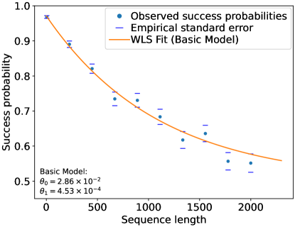
(a) Uniform design, repeated sequences

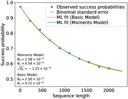
(b) Uniform design, fully randomized

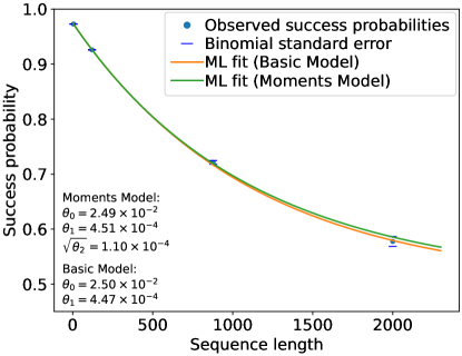
(c) Optimized design, fully randomized

Figure 6: The observed decays in success probability for each of the three experiments where we intentionally introduced coherent errors. The experiment in plot (a) has sequence lengths chosen uniformly in the range [5,2000] and for each sequence length $100$ random sequences ar drawn and run $100$ times each. The experiment in plot (b) has the same sequence lengths as the first experiment, but is fully randomized so at each sequence length $100\times 100$ random sequences are drawn and run once each. Each of the three experiments takes the same total time of approximately $40$ minutes. All other aspects of the plots are the same as in Fig. 3.

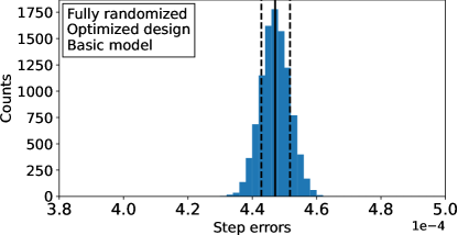
(a)

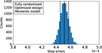
(b)

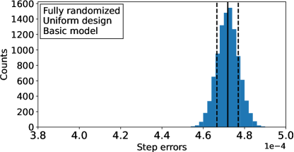
(c)

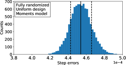
(d)

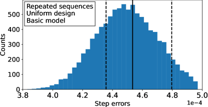
(e)

Figure 7: The bootstrap distributions obtained during the analysis of the three experiments we ran during the comparison where we intentionally introduced coherent errors. All aspects of the plots are the same as in Fig. 4. The best fit step errors for the plots are (a) $4.47^{+0.05}_{-0.04}\times 10^{-4}$, (b) $4.51^{+0.06}_{-0.06}\times 10^{-4}$, (c) $4.72^{+0.05}_{-0.05}\times 10^{-4}$, (d) $4.54^{+0.12}_{-0.11}\times 10^{-4}$, (e) $4.53^{+0.26}_{-0.18}\times 10^{-4}$.

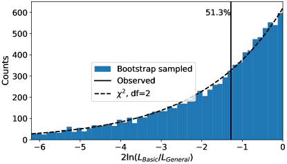
Figure 8: Results of an empirical likelihood ratio test for the optimized, fully randomized experiment. We perform the procedure described in Section 7, with the basic model as the inner model and the general model as the outer model. We find a p-value to reject the basic model of $51.3\%$, which indicates little evidence for rejection. All other aspects of the plots are the same as in Fig. 5.

9 Conclusion

In this work we study fully randomized benchmarking, where a new random sequence is drawn independently for each trial. We analyze the concrete advantages of fully randomized benchmarking, which include smaller error bars on the inferred step error, maximum likelihood analysis without heuristics, straightforward optimization of the sequence lengths, insensitivity to drifts in SPAM throughout the experiment, and the ability to model and measure behaviors such beyond the basic randomized benchmarking model usually assumed, such as gate-position-dependent errors or time-drifting errors. Furthermore, we provide a general formulation of statistical models for fully randomized benchmarking and give a procedure to optimize the design of the experiment to minimize the uncertainty of inference of a particular model parameter, typically the step error. This optimization can be done for an arbitrary statistical model that can be linearized around a reference point, and takes into account the actual wall-clock time of running a random sequence of each possible length. For experiments that are not fully randomized, we analyze the dependence of the uncertainty on the number of times that each sequence is repeated and show concrete advantages from fully randomizing. We also discuss the moments model of fully randomized benchmarking and show that it is a general model of time-dependent errors when constraints on the moments parameters are removed. We show how an empirical likelihood ratio test can be used to possibly distinguish the basic model of a single exponential decay from more general models. Finally, we implement fully randomized benchmarking on a trapped ion qubit at NIST and run experiments that allows us to compare optimized, fully randomized benchmarking to randomized benchmarking with uniform sequence lengths and intentionally repeated sequences. We find substantial reductions in the uncertainty in the estimated step error as a result of fully randomizing.

Appendix A Computing optimal linear estimators for a given experiment design

If the experiment design is fixed, the coefficients $\left(C_{n}\right)$ of the optimal linear estimator for a parameter $\theta_{i_{0}}$ at the reference point $\bm{\theta}^{(0)}$ can be computed as follows. In the notation of Section 3, the goal is to minimize the variance in Eq. 3.5, which is $v=\sum_{n}\frac{C_{n}^{2}v_{n}}{w_{n}}$, subject to the linear constraints $\sum_{n}C_{n}L_{ni}=\delta_{ii_{0}}$. This is a quadratic program with linear constraints and can be written in matrix notation as a minimization of $\mathbf{c}^{\top}Q\mathbf{c}$ subject to $E\mathbf{c}=\mathbf{d}$, where $\mathbf{c}$ is the list of coefficients $\left(C_{n}\right)$ in vector form, $Q$ is a diagonal matrix with diagonal elements $Q_{nn}=\frac{v_{n}}{w_{n}}$, the constraint matrix $E$ has elements $E_{in}=L_{ni}$, and $d_{i}=\delta_{ii_{0}}$. The solution for $\mathbf{c}$ can be obtained by solving

$$\matrixquantity[Q&E^{\top}\\ E&0]\matrixquantity[\mathbf{c}\\ \mathbf{\lambda}]=\matrixquantity[0\\ \mathbf{d}]$$ (A.1)

where $\mathbf{\lambda}$ is a vector of Lagrange multipliers [53]. This can be achieved by using the standard formula for the inverse of a block matrix [53, 54], and the solution for $\mathbf{c}$ is

$$\mathbf{c}=Q^{-1}E^{\top}(EQ^{-1}E^{\top})^{-1}\mathbf{d}.$$ (A.2)

As a result, the $i$th column of the matrix $M=Q^{-1}E^{\top}(EQ^{-1}E^{\top})^{-1}$ has the coefficients of the optimal linear estimator for the $i$th parameter $\theta_{i}$.

Appendix B Interpretation of design optimization in the context of Fisher information

For a given experiment design and reference point $\bm{\theta}^{(0)}$, we show that the covariance matrix $V$ of the optimal linear estimators obtained in Appendix A is equal to the inverse of the Fisher information matrix. This is well established in the literature on experiment design and Fisher information [32, 55, 35, 31], and for convenience we provide a derivation here. As we show in Appendix A, the $i$th column of the matrix $M=Q^{-1}E^{\top}(EQ^{-1}E^{\top})^{-1}$ has the coefficients of the optimal linear estimator for the $i$th parameter $\theta_{i}$. Therefore, the covariance matrix $V$ of these linear estimators satisfies $V=M^{\top}QM$, which evaluates to

$$V=M^{\top}QM=(EQ^{-1}E^{\top})^{-1\top}EQ^{-1}QQ^{-1}E^{\top}(EQ^{-1}E^{\top})^{-1}.$$ (B.1)

The matrix $Q$ is diagonal, so we have $(EQ^{-1}E^{\top})^{-1\top}=(EQ^{-1}E^{\top})^{-1}$, and this simplifies to

$$V=(EQ^{-1}E^{\top})^{-1}.$$ (B.2)

The Fisher information matrix for a single trial of sequence length $n$ can be obtained according to the standard formula [32]

$$F_{ii^{\prime}}(n)=\bigg{<}\frac{\partial}{\partial\theta_{i}}\log{p}\frac{\partial}{\partial\theta_{i^{\prime}}}\log{p}\bigg{>}_{\bm{\theta}^{(0)}},$$ (B.3)

where the expectation value is taken over the two measurement outcomes ‘success’ and ‘failure’, and $p$ is the likelihood of getting a particular outcome. The subscript $\bm{\theta}^{(0)}$ indicates that the formula is evaluated at the reference point $\bm{\theta}^{(0)}$. Evaluating this for the two-outcome measurement for a single trial of sequence length $n$ gives

$$F_{ii^{\prime}}(n)= \left.P_{\bm{\theta}}(n)\frac{\partial}{\partial\theta_{i}}\log\left[P_{\bm{\theta}}(n)\right]\frac{\partial}{\partial\theta_{i^{\prime}}}\log\left[P_{\bm{\theta}}(n)\right]\right|_{\bm{\theta}^{(0)}}+$$

$$\left.\left[1-P_{\bm{\theta}}(n)\right]\frac{\partial}{\partial\theta_{i}}\log\left[1-P_{\bm{\theta}}(n)\right]\frac{\partial}{\partial\theta_{i^{\prime}}}\log\left[1-P_{\bm{\theta}}(n)\right]\right|_{\bm{\theta}^{(0)}}.$$ (B.4)

Using the fact that $\left.E_{ni}=\frac{\partial}{\partial\theta_{i}}P_{\bm{\theta}}(n)\right|_{\bm{\theta}^{(0)}}$, this simplifies to

$$F_{ii^{\prime}}(n)=\frac{E_{ni}E_{ni^{\prime}}}{P_{\bm{\theta}^{(0)}}(n)(1-P_{\bm{\theta}^{(0)}}(n))}.$$ (B.5)

Weighting by the number of trials $w_{n}$ at sequence length $n$ and summing over $n$ gives a total Fisher information matrix of

$$F_{ii^{\prime}}=\sum_{n}\frac{E_{ni}w_{n}E_{i^{\prime}n}}{P_{\bm{\theta}^{(0)}}(n)(1-P_{\bm{\theta}^{(0)}}(n))}.$$ (B.6)

Using the fact that, as in Section 3, the matrix $Q$ is diagonal with entries $Q_{nn}=w_{n}/v_{n}$ with $v_{n}=[P_{\bm{\theta}^{(0)}}(n)(1-P_{\bm{\theta}^{(0)}}(n))]$, this simplifies to $F=EQ^{-1}E^{\top}$. Therefore, comparison to Eq. B.2 shows that the covariance matrix of the optimal linear estimators $V$ is equal to the inverse of the Fisher information matrix $F$. In this sense, the optimization procedure described in Section 3 is Fisher-optimal.

Appendix C Details of variance analysis of fully randomized benchmarking

Here we verify the fact that

$$\int d\psi_{H}f_{\psi}^{2}=\frac{2}{D(D+1)},$$ (C.1)

where $d\psi_{H}$ denotes the Haar measure over pure states, and $f_{\psi}$ is the fidelity of the random pure state $\ket{\psi}$ with the target state $\ket{\chi}$. The Haar-random pure state $\ket{\psi}$ can be expressed as $U\ket{\chi}$ for a Haar-random unitary $U$, so this integral can be written as

$$\int d\psi_{H}f_{\psi}^{2}=\int dU_{H}\text{tr}\left[(U\otimes U)\outerproduct{\chi}{\chi}^{\otimes 2}(U^{\dagger}\otimes U^{\dagger})\outerproduct{\chi}{\chi}^{\otimes 2}\right].$$ (C.2)

In the notation of Lemma 3.5 of Ref. [56], we can express this as

$$\int d\psi_{H}f_{\psi}^{2}=\text{tr}\left[E(M)M\right],$$ (C.3)

where $M=\outerproduct{\chi}{\chi}^{\otimes 2}$ and $E(M)$ is defined to be

$$E(M)=\int dU_{H}(U\otimes U)M(U^{\dagger}\otimes U^{\dagger}).$$ (C.4)

According to Prop. 2.2 in Ref. [57] and Lemma 3.5 in Ref. [56], it follows from Schur-Weyl duality that

$$E(M)=\alpha\mathbb{1}+\beta F,$$ (C.5)

where $F$ is the swap operator and the coefficients $\alpha,\beta$ satisfy $\alpha D^{2}+\beta D=\text{tr}\left[M\right]$ and $\alpha D+\beta D^{2}=\text{tr}\left[MF\right]$. Here we have $M=\outerproduct{\chi}{\chi}^{\otimes 2}$ so $\text{tr}\left[M\right]=\text{tr}\left[MF\right]=1$ and it follows that $\alpha=\beta=\frac{1}{D(D+1)}$. Consequently, $\text{tr}\left[E(M)M\right]=\frac{2}{D(D+1)}$.