Trees of Graphs as Boundaries of Hyperbolic Groups

Abstract.

We characterize those 1-ended word hyperbolic groups whose Gromov boundaries are homeomorphic to trees of graphs, the family of simplest connected 1-dimensional spaces appearing among Gromov boundaries. The characterization refers to the features of the Bowditch JSJ splitting of the corresponding groups (i.e their canonical JSJ splitting over 2-ended subgroups).

1. Introduction

In this paper we address the following classical and widely open problems:

1. to describe explicitely the class of topological spaces which appear as Gromov boundaries of word hyperbolic groups, and

2. to characterize those word hyperbolic groups whose Gromov boundary is homeomorphic to a given topological space.

Concerning the above problem (1), the paper [22] provides its reduction to the case when the boundary is connected, i.e. the corresponding group is 1-ended. Some further partial insight into problem (1) is provided in [18], by showing that Gromov boundaries of hyperbolic groups belong to the class of topological spaces called Markov compacta. These are, roughly speaking, the spaces which can be realized as inverse limits of sequences of polyhedra built recursively out of an initial finite polyhedron according to some finite set of modification rules. In dimension 1, the easiest to describe reasonably rich class of Markov compacta is that of so called regular trees of graphs, as introduced in Section 6 of this paper. The main result of this paper is the complete characterization of those 1-ended hyperbolic groups $G$ whose Gromov boundaries $\partial G$ are trees of graphs (see Theorem A below).

In the statement of our main result, we refer to the concept of a regular tree of graphs (as mentioned above), as well as to the more general concept of a tree of graphs, as introduced in Section 4. The statement refers also to some features of the Bowditch JSJ splitting of a group $G$, as introduced in [1], and recalled in detail in Section 3. This is a particular canonical splitting of $G$ over 2-ended subgroups. It is defined when $G$ is not cocompact Fuchsian. ($G$ is cocompact Fuchsian if it acts properly and cocompactly on the hyperbolic plane, a condition equivalent to $\partial G\cong S^{1}$.) Here we mention only few details concerning the Bowditch JSJ splitting, which are necessary for the statement of Theorem A.

Technically, the Bowditch JSJ splitting of $G$ is the action of $G$ on the associated Bass-Serre tree ${T}_{G}$, called the Bowditch JSJ tree for $G$. This tree is naturally bipartitioned into black and white vertices. The black vertices are either rigid or flexible, and their stabilizers are the essential factors of the splitting (which are also called rigid and flexible, respectively). The white vertex stabilizers are the maximal 2-ended subgroups of $G$. The $G$-action on ${T}_{G}$ preserves all the above mentioned types of the vertices. We introduce the notion of a rigid cluster in $T_{G}$, as follows. We say that some two rigid vertices in $T_{G}$ are adjacent if their combinatorial distance in $T_{G}$ is equal to 2. A rigid cluster is a subtree of $T_{G}$ spanned on any equivalence class of the equivalence relation on the set of rigid vertices of $T_{G}$ induced by the adjacency. A rigid cluster factor of $G$ is the stabilizing subgroup of any rigid cluster, i.e. the subgroup consisting of all elements which map this cluster to itself. In particular, any rigid factor of $G$ is contained in some rigid cluster factor, but in general rigid cluster factors are larger than rigid factors, and they are in some sense ”combined” of some collections of rigid factors. See Subsection 3.2, and in particular Remark 3.6, for more detailed explanations, and for the description of a related splitting that we call the reduced Bowditch JSJ splitting of $G$.

Recall finally that a graph is 2-connected if it is finite, connected, nonempty, not reduced to a single vertex, and contains no cutpoint.

Theorem A.

Let $G$ be a 1-ended hyperbolic group that is not cocompact Fuchsian. Then the following conditions are equivalent:

1. $\partial G$ is homeomorphic to a tree of graphs;

2. $\partial G$ is homeomorphic to a regular tree of 2-connected graphs;

3. each rigid cluster factor of $G$ is virtually free.

As a complement to Theorem A, we present also in the paper the description of the structure of a regular tree of graphs appearing in condition (2) of this result, given explicitely in terms of the features of the corresponding Bowditch JSJ splitting of $G$ (see Theorem 10.1, and the description of the corresponding graphical connecting system $\mathcal{R}_{G}$ given in Section 10).

One can view Theorem A as confirming that regular trees of graphs are indeed the simplest topological spaces in the complexity hierarchy among connected 1-dimensional Gromov boundaries of hyperbolic groups. Theorem A shows also that the zoo of connected 1-dimensional Gromov boundaries is quite complicated, and there is a big gap in it between trees of graphs and the boundaries of those groups which contain as their rigid factors groups whose boundary is either the Sierpinski curve or the Menger curve. The closer understanding of the species inside this gap seems to be an interesting challenge for future investigations.

As a byproduct of the methods developed for the proof of Theorem A, we present also another result, Theorem B below. In the light of the comments in the previous paragraph, it can be viewed as characterizing those 1-ended hyperbolic groups $G$ whose boundaries $\partial G$ belong to some subclass in the class of trees of graphs, which consists of the simplest spaces among them, namely the so called trees of $\theta$-graphs. A $\theta$-graph is any connected graph having precisely 2 vertices, whose any edge has both these vertices as its endpoints (obviously, $\theta$-graphs typically contain multiple edges). A $\theta$-graph is thick if it has at least three edges. A tree of thick $\theta$-graphs is a tree of graphs whose all consituent graphs are thick $\theta$-graphs (compare Section 4).

Theorem B.

Let $G$ be a 1-ended hyperbolic group that is not cocompact Fuchsian. Then the following conditions are equivelent:

1. $\partial G$ is homeomorphic to a tree of thick $\theta$-graphs;

2. $\partial G$ is homeomorphic to a regular tree of thick $\theta$-graphs;

3. $G$ has no rigid factor in its (Bowditch) JSJ splitting.

1.1. Examples.

We now illustrate our results with few examples (see Figures 1-4). The details concerning these examples, and other examples of a different nature, will be discussed and presented in Section 14. In each of the examples below the 1-ended hyperbolic group $G_{i}$ is the fundamental group of the corresponding ”graph of surfaces” $M_{i}$. Recall also that the Bowditch JSJ splitting of a group $G$ (as well as its reduced Bowditch JSJ splitting) can be expressed by means of the related graph of groups decomposition $\mathcal{G}$ of $G$, and this is the approach that we follow below. In all four discussed examples $G_{i}$, $i\in\{1,2,3,4\}$, the edge groups of the corresponding graph of groups decompositions $\mathcal{G}_{i}$ coincide with the corresponding incident white vertex groups, so we skip the indication of the form of these edge groups at the figures.

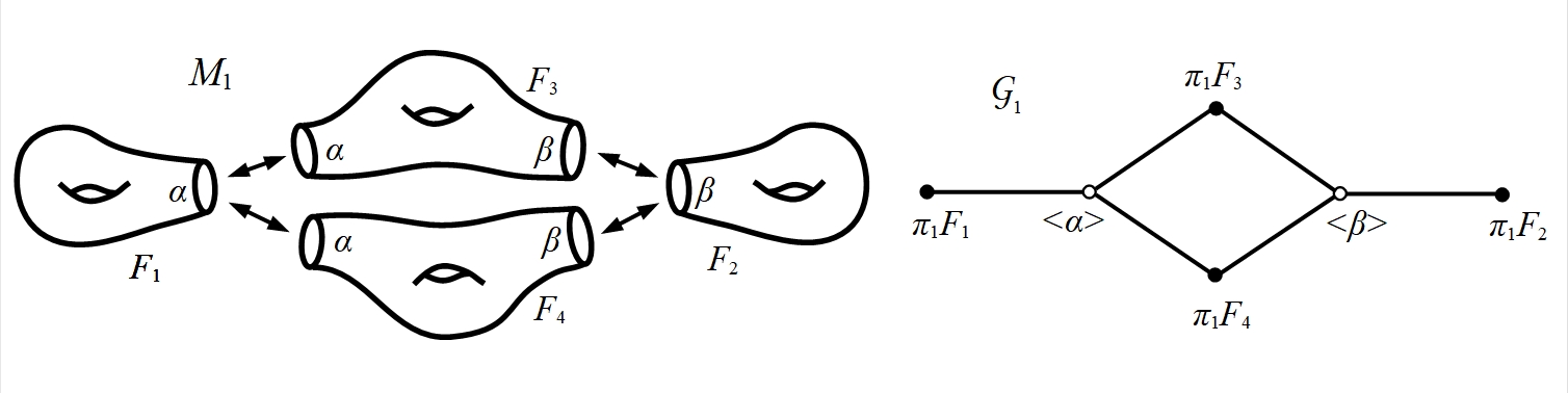
Figure 1. “Graph of surfaces” $M_{1}$ and JSJ splitting $\mathcal{G}_{1}$ of its fundamental group $G_{1}=\pi_{1}M_{1}$.

Consider the group $G_{1}=\pi_{1}M_{1}$, presented at Figure 1. The Bowditch JSJ graph of groups decomposition of $G_{1}$, denoted $\mathcal{G}_{1}$, is presented at the right part of this figure. Since all factors of this decomposition are easily seen to be flexible (because they are the conjugates of the surface subgroups $\pi_{1}F_{i}$ equipped with peripheral subgroups corresponding to the boundary curves), condition (3) of Theorem B holds for $G_{1}$, and hence the boundary $\partial G_{1}$ is homeomorphic to some regular tree of thick $\theta$-graphs.

Figure 2 shows an example in which the corresponding group $G_{2}=\pi_{1}M_{2}$ contains, up to conjugacy, precisely one rigid factor in its Bowditch JSJ splitting. This factor corresponds to the subgroup $\pi_{1}H_{0}<\pi_{1}M_{2}$, and it is obviously isomorphic to the free group of rank 2. Moreover, it is not hard to observe that the rigid clusters in the Bowditsch’s JSJ tree of $G_{2}$ coincide with the rigid vertices, and hence the rigid cluster factors coincide with the rigid factors (actually, in this case the reduced Bowditch JSJ splitting coincides with the ordinary Bowditch JSJ splitting). It follows that the group $G_{2}$ satisfies condition (3) of Theorem A, and hence its Gromov boundary $\partial G_{2}$ is homeomorphic to some regular tree of 2-connected graphs. In Section 14 we will give a complete description of this regular tree of graphs, in terms of the so called graphical connecting system $\mathcal{R}_{G_{2}}$ associated to $G_{2}$ in the way presented in Section 10.

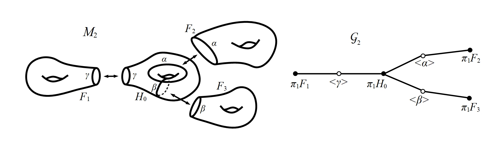
Figure 2. “Graph of surfaces” $M_{2}$ and JSJ splitting $\mathcal{G}_{2}$ of its fundamental group $G_{2}=\pi_{1}M_{2}$.

The group $G_{3}=\pi_{1}M_{3}$ presented at Figure 3 contains, up to conjugacy, precisely two rigid factors in its Bowditch JSJ splitting, and they correspond to the subgroups $\pi_{1}H_{i}<\pi_{1}M_{3}$, $i=1,2$. It can be deduced from the corresponding graph of groups decomposition $\mathcal{G}_{3}$ of $G_{3}$ that the rigid clusters are in this case nontrivial, and that the rigid cluster factors of $G_{3}$ are the conjugates of the subgroup $\pi_{1}(H_{1}\cup H_{2})$. (The corresponding reduced Bowditch JSJ graph of groups decomposition of $G_{3}$ is presented as $\mathcal{G}^{r}_{3}$ at the same figure.) Since obviously these rigid cluster factors are free, condition (3) of Theorem A is again satisfied, and thus the boundary $\partial G_{3}$ is also homeomorphic to some regular tree of 2-connected graphs.

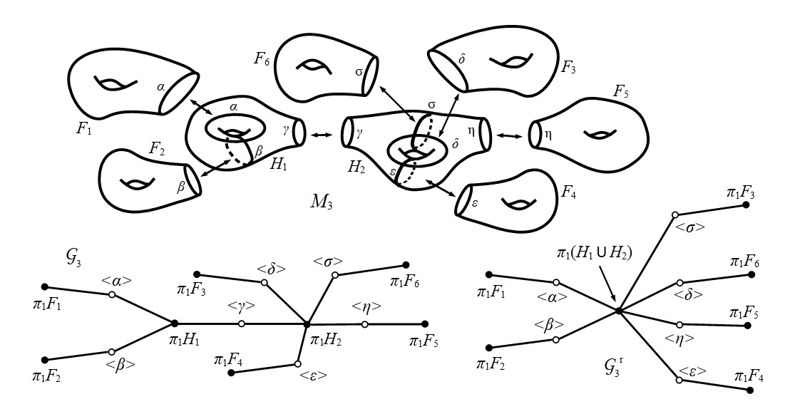
Figure 3. “Graph of surfaces” $M_{3}$ and splittings $\mathcal{G}_{3}$ and $\mathcal{G}_{3}^{r}$ of its fundamental group $G_{3}=\pi_{1}M_{3}$.

Our final example, presented at Figure 4, shows some 1-ended hyperbolic group $G_{4}=\pi_{1}M_{4}$ whose boundary $\partial G_{4}$ is not a tree of graphs, even though its all rigid factors are free. The rigid factors of $G_{4}$ correspond to the subgroups $\pi_{1}H_{i}<\pi_{1}M_{4}$, for $i=1,2$, and the rigid cluster factors correspond to the subgroup $\pi_{1}(H_{1}\cup H_{2})$. Since that latter group is the fundamental group of a closed surface, it is not virtually free, and hence condition (3) of Theorem A is not fulfilled. As a consequence, the boundary $\partial G_{4}$ is not homeomorphic to any tree of graphs.

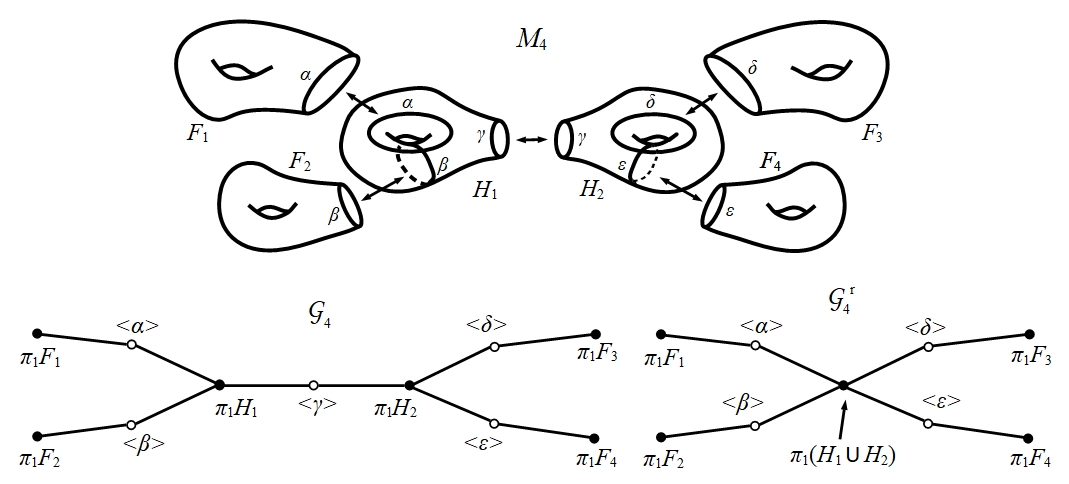
Figure 4. “Graph of surfaces” $M_{4}$ and splittings $\mathcal{G}_{4}$ and $\mathcal{G}_{4}^{r}$ of its fundamental group $G_{4}=\pi_{1}M_{4}$.

1.2. Organization of the paper.

The paper is organized as follows. The first part of the paper (Sections 2–5) focuses on the proofs of the implications (1)$\implies$(3) in Theorem A, and (1)$\implies$(3) in Theorem B. The second part of the paper (Sections 6–13) deals with the proofs of the implications (3)$\implies$(2) in Theorem A, and (3)$\implies$(2) in Theorem B. The remaining implications ((2)$\implies$(1) in Theorem A, and (2)$\implies$(1) in Theorem B) necessary to get the full proofs of Theorems A and B are obvious.

Our exposition in both parts of the paper consists of many preparations for the proofs, including the complete descriptions and explanations of the terms appearing in the statements of our two main results. More precisely, as far as the first part, the organization is as follows. In Section 2 we recall the construction called the limit of a tree system of metric compacta. It is used later, in Section 4, to describe trees of graphs (and trees of $\theta$-graphs), and it is also used throughout the paper, as the main technical ingredient in the arguments. In Section 3 we recall the concept of the canonical (Bowditch) JSJ splitting of a 1-ended hyperbolic group, and we describe related concepts of the reduced Bowditch JSJ splitting, and of rigid cluster factors of this reduced splitting. In Section 5 we study some configurations of local cutpoints in trees of graphs (and trees of $\theta$-graphs), and we deduce the proofs of the implications (1)$\implies$(3) in Theorem A, and (1)$\implies$(3) in Theorem B.

As far as the second part of the paper, the organization is as follows. In Section 6 we introduce regular trees of graphs. Sections 7–9 provide various technicalities and terminology which allow to state in Section 10 (as Theorem 10.1) the result which describes explicitely the form of the regular trees of graphs which appear in our main results. In particular, we discuss in Section 9 some graphs (the so called Whitehead graphs, and their extended variants) which are naturally associated to those rigid factors (or rather rigid cluster factors) of the JSJ splittings which are virtually free. Sections 10–12 contain some further technical preparations, and in Section 13 we present the proofs of those parts of Theorems A and B, which identify the Gromov boundaries of the corresponding groups as explicitely described regular trees of graphs.

Finally, in Section 14, we discuss the examples presented above in this introduction, as well as some further examples, of a different sort, namely some right-angled Coxeter groups.

2. Tree systems and their limits

In this preparatory section we present (or rather recall) the construction called limit of a tree system of spaces (or, less formally, a tree of spaces). This construction is a slight extension of that presented in Section 1 of [23] (see also [19]). We will use this construction in the next sections to describe and study trees of graphs, the class of spaces on which we focus in this paper.

2.1. Some terminology and notation concerning trees

We will mainly deal with trees $T$ where the vertex set $V_{T}$ is endowed with a bipartition $V_{T}=V_{T}^{b}\sqcup V_{T}^{w}$ into black and white vertices such that every edge of $T$ has endpoints of different colours. We denote the set of all (unoriented) edges of $T$ by $E_{T}$, and for each $e\in E_{T}$ we denote by $b(e)$ and $w(e)$ the black and the white endpoint of $e$, respectively. We will usually denote black vertices with letters $t,s$ and white ones with $u,w$. We use also other letters, such as $v,z,x,y$, to denote vertices whose colour is not essential.

We denote by $[v,z]$ the combinatorial (embedded) path in $T$ connecting a vertex $v$ to a vertex $z$. (If $v,z$ are adjacent, $[v,z]$ denotes also the edge with the endpoints $v,z$.) A ray in $T$ is an infinite (embedded) combinatorial path having an initial vertex. We usually denote rays by $\rho$, and we denote by $\rho(0)$ the initial vertex and by $e_{1}(\rho)$ the initial (unoriented) edge of a ray $\rho$.

For any $v\in V_{T}$, we denote by $N^{T}_{v}$, or simply by $N_{v}$, the set of all vertices of $T$ adjacent to $v$. We denote by $d(v)=d_{T}(v)$ the degree of a vertex $v$ in $T$, i.e. the cardinality of the set $N^{T}_{v}$.

We denote by $\partial T$ the set of ends of $T$, i.e. the set of equivalence classes of rays in $T$ with respect to the relation of coincidence except possibly at some finite initial parts. We denote the end determined by a ray $\rho$ as $[\rho]$.

We consider subtrees of $T$ of some special form, that we call b-subtrees. A subtree $S$ of $T$ is a b-subtree if for each white vertex $u$ of $S$ the set $N^{T}_{u}$ is contained in the vertex set of $S$. We apply to b-subtrees $S$ the earlier introduced notation $V_{S}$, $V_{S}^{b}$, $V_{S}^{w}$, $E_{S}$, $N^{S}_{v}$, $d_{S}(v)$, etc. For a b-subtree $S$ of $T$ we define

$$N_{S}=\{u\in V_{T}:\text{$u\notin V_{S}$ and $u$ is adjacent to some $t\in V_{S}$}\}.$$

Note that $N_{S}$ consists solely of white vertices of $T$. Note also that, in case when $S$ is reduced to a single black vertex $t$, this notation agrees with the earlier introduced notation for the set $N_{t}$.

2.2. Spaces with peripherals and tree systems

Recall that a family of subsets of a compact metric space is null if for each $\varepsilon>0$ all but finitely many of these subsets have diameters less than $\varepsilon$. Note that nullness of a family of subspaces does not depend on the choice of a metric compatible with the topology of the corresponding space.

Definition 2.1.

A space with peripherals is a pair $(K,\Omega)$ such that $K$ is a compact metric space and $\Omega$ is a countable null family of pairwise disjoint closed subsets of $K$. We call the sets from $\Omega$ the peripheral subspaces of $K$, or simply the peripherals of $K$.

Example 2.2.

Say that a graph $\Gamma$ is essential if it is nonempty and contains no isolated vertex. (We allow that $\Gamma$ contains loop edges and multiple edges.) Given a finite essential graph $\Gamma$, we describe the associated space with peripherals called the punctured graph $\Gamma$, denoted $\Gamma^{\circ}$, as follows. Denote by $|\Gamma|$ the realization of $\Gamma$, i.e. the underlying topological space of $\Gamma$, which is a compact metric space. For each point $x\in|\Gamma|$ consider a normal neighbourhood of $x$ in $\Gamma$, i.e. a connected closed neighbourhood $B(x)$ of $x$ whose intersection with the vertex set of $\Gamma$ either coincides with $\{x\}$ (when $x$ is a vertex of $\Gamma$), or is empty. Denote by $\operatorname{int}B(x)$ and $\operatorname{bd}B(x)$ the interior and the boundary (in $|\Gamma|$) of a normal neighbourhood $B(x)$, respectively. A standard dense family of normal neighbourhoods in $\Gamma$ is any family of pairwise disjoint normal neighbourhoods in $\Gamma$ which contains normal neighbourhoods of all vertices of $\Gamma$, and whose union is dense in $|\Gamma|$. Note that each such family is automatically countable and null. Moreover, such family is unique up to a homeomorphism of the ambient space $|\Gamma|$ which is identical on the vertex set of $\Gamma$ and which maps all edges of $\Gamma$ to themselves.

Let ${\mathcal{N}}_{\Gamma}$ be a standard dense family of normal neighbourhoods in $\Gamma$. Put

$$\Gamma^{\circ}:=|\Gamma|\setminus\bigcup\{\operatorname{int}B:B\in{\mathcal{N}}_{\Gamma}\}$$

and

$$\Omega=\{\operatorname{bd}B:B\in{\mathcal{N}}_{\Gamma}\}.$$

Note that, by what was said above, $\Gamma^{\circ}$ is a compact metric space, and $\Omega$ is a countable and null family of closed subsets of $\Gamma^{\circ}$. The punctured graph $\Gamma$ is the space with peripherals $(\Gamma^{\circ},\Omega)$.

Note that the peripheral sets $\operatorname{bd}B(x)$ of $\Gamma^{\circ}$ naturally correspond to vertices and edges of $\Gamma$, according to whether $x$ is a vertex or an interior point of an edge. This correspondence describes what we call a type of a peripheral set. The space with peripherals $(\Gamma^{\circ},\Omega)$ is unique up to a homeomorphism which respects types of peripheral sets.

If the underlying space $|\Gamma|$ of a graph $\Gamma$ is homeomorphic to the circle $S^{1}$, it is not hard to realize that the space with peripherals $(\Gamma^{\circ},\Omega)$ as above does not depend, up to homeomorphism, on the number of edges in $\Gamma$. This justifies the notation $(S^{1})^{\circ}$ for this space with peripherals, and the term punctured circle, with which we will be referring to it later.

Punctured graphs will be used in the next section, to describe trees of graphs.

Definition 2.3.

A tree system of spaces is a tuple $\Theta=(T,\{K_{t}\},\{\Sigma_{u}\},\{\varphi_{e}\})$ such that:

1. $T$ is a bipartite countable tree (called the underlying tree of $\Theta$), with black and white vertices of the partition, such that the degree $d(u)$ of each white vertex $u$ is finite;

2. to each black vertex $t\in V_{T}^{b}$ there is associated a nonempty compact metric space $K_{t}$, called a constituent space of $\Theta$;

3. to each white vertex $u\in V_{T}^{w}$ there is associated a nonempty compact metric space $\Sigma_{u}$, called a peripheral space of $\Theta$;

4. to each edge $e\in E_{T}$ there is associated a topological embedding

   $$\varphi_{e}:\Sigma_{w(e)}\to K_{b(e)},$$

   called a connecting map of $\Theta$;

5. for each black vertex $t\in V_{T}^{b}$ the pair

   $$(K_{t},\{\varphi_{[t,u]}(\Sigma_{u}):u\in N_{t}\})$$

   is a space with peripherals, i.e. the family $\Omega_{t}:=\{\varphi_{[t,u]}(\Sigma_{u}):u\in N_{t}\}$ is null and consists of pairwise disjoint sets; pairs $(K_{t},\Omega_{t})$ are called the constituent spaces with peripherals of $\Theta$.

Note that, by condition (TS5), a black vertex of the underlying tree $T$ of a system $\Theta$ typically has infinite (countable) degree.

2.3. Limit of a tree system

We now describe, following the exposition in Section 1 of [23], an object called the limit of a tree system $\Theta=(T,\{K_{t}\},\{\Sigma_{u}\},\{\varphi_{e}\})$, denoted $\lim\Theta$, starting with its description as a set. Denote by $\#\Theta$ the quotient

$$(\bigsqcup_{t\in V_{T}^{b}}K_{t})/\sim$$

of the disjoint union of the sets $K_{t}$ by the equivalence relation $\sim$ induced by the equivalences $\varphi_{[u,t]}(x)\sim\varphi_{[u,s]}(x)$ for any $u\in V_{T}^{w}$, any $x\in\Sigma_{u}$, and any vertices $t,s\in N_{u}$. This set may be viewed as obtained from the family $K_{t}:t\in V$ as a result of gluings provided by the maps

$$\varphi_{[u,s]}\varphi_{[u,t]}^{-1}:\varphi_{[u,t]}(\Sigma_{u})\to\varphi_{[u,s]}(\Sigma_{u}).$$

Observe that, by the fact that the peripheral subspaces in any $K_{t}$ are pairwise disjoint, the equivalence classes of the relation $\sim$ are easy to describe, and they are all finite (some of them have cardinality 1, and others have cardinalities equal to the degrees of the appropriate white vertices of $T$). Observe also that any set $K_{t}$ canonically injects in $\#\Theta$. Define $\lim\Theta$ to be the disjoint union $\#\Theta\sqcup\partial T$, where $\partial T$ is the set of ends of $T$.

To put appropriate topology on the set $\lim\Theta$ we need more terminology. Given a family $\mathcal{A}$ of subsets in a set $X$, we say that $U\subset X$ is saturated with respect to $\mathcal{A}$ (shortly, $\mathcal{A}$-saturated) if for any $A\in{\mathcal{A}}$ we have either $A\subset U$ or $A\cap U=\emptyset$.

For any finite b-subtree $F$ of $T$, denote by

$$\Theta_{F}=(F,\{K_{t}:t\in V_{F}^{b}\},\{\Sigma_{u}:u\in V_{F}^{w}\},\{\varphi_{e}:e\in E_{F}\})$$

the tree system $\Theta$ restricted to $F$. The set $K_{F}:=\#\Theta_{F}$, equipped with the natural quotient topology (with which it is clearly a metrizable compact space), will be called the partial union of the system $\Theta$ related to $F$. Observe that any partial union $K_{F}$ is canonically a subset in $\#\Theta$, and thus also in $\lim\Theta$.

For any finite b-subtree $F$ and for any $u\in N_{F}$ denote by $t_{u}$ the (unique) vertex of $F$ adjacent to $u$ (which is necessarily a black vertex). Put ${\Omega}_{F}=\{\varphi_{[u,t_{u}]}(\Sigma_{u}):u\in N_{F}\}$, and view the elements of this family as subsets in the partial union $K_{F}$. Observe that the family ${\Omega}_{F}$ consists of pairwise disjoint closed subsets, and that this family is countable and null (so that $(K_{F},\Omega_{F})$ is a space with peripherals). Let $U\subset K_{F}$ be a subset which is saturated with respect to $\Omega_{F}$. Put $N_{U}:=\{u\in N_{F}:\varphi_{[u,t_{u}]}(\Sigma_{u})\subset U\}$ and

$$D_{U}:=\{t\in V_{T}^{b}:\text{$[u,t]\cap F=\emptyset$ for some $u\in N_{U}$}\}$$

(i.e. $D_{U}$ is the set of these vertices $t\in V_{T}^{b}\setminus V_{F}$ for which the shortest path in $T$ connecting $t$ to $F$ passes through a vertex $u\in N_{U}$).

Again, for any finite b-subtree $F$ of $T$ let $R_{F}$ be the set of all rays $\rho$ in $T$ with $\rho(0)\in N_{F}$, and disjoint with $F$. Note that the map $\rho\to[\rho]$ is then a bijection from $R_{F}$ to the set $\partial T$ of all ends of $T$. Given a subset $U\subset K_{F}$ as above (i.e. saturated with respect to $\Omega_{F}$), put

$$R_{U}:=\{\rho\in R_{F}:\rho(0)\in N_{U}\},$$

and put also $\partial_{U}:=\{[\rho]\in\partial T:\rho\in R_{U}\}$.

Finally, for any subset $U\subset K_{F}$ as above, put

$${\mathcal{G}}(U):=U\cup(\bigcup_{t\in D_{U}}K_{t})\cup\partial_{U},$$

where all summands in the above union are viewed as subsets of $\lim\Theta$; clearly, ${\mathcal{G}}(U)$ is then also a subset in $\lim\Theta$. We consider the topology in the set $\lim\Theta$ given by the basis $\mathcal{B}$ consisting of all sets ${\mathcal{G}}(U)$, for all finite b-subtrees $F$ in $T$, and all open subsets $U\subset K_{F}$ saturated with respect to $\Omega_{F}$. We leave it as an easy and instructive exercise to check that the family $\mathcal{B}$ is closed under finite intersections, and hence it satisfies the axioms for a basis of topology. Moreover, we have the following result, which is a slight extension of Proposition 1.C.1 of [23], and which can be justified by the same proof as the latter proposition.

Proposition 2.4.

For any tree system $\Theta$ of metric compacta the limit $\lim\Theta$, with topology given by the above described basis $\mathcal{B}$, is a compact metrizable space.

2.4. Functoriality with respect to subtrees

A tree system can be naturally restricted to any b-subtree of the underlying tree. Namely, let $S\subset T$ be a b-subtree of $T$. The restriction of $\Theta$ to $S$ is the tree system

$$\Theta_{S}=(S,\{K_{t}:t\in V_{S}^{b}\},\{\Sigma_{u}:u\in V_{S}^{w}\},\{\varphi_{e}:e\in E_{S}\}).$$

Next observation follows by a direct argument (compare the proof of Claim 1 inside the proof of Theorem 3.A.1 in [23]).

Fact 2.5.

The natural map $\#\Theta_{S}\cup\partial_{S}\to\#\Theta\cup\partial_{T}$ induced by the inclusion $S\to T$, and by the identities of the spaces $K_{t}:t\in V_{S}$, is injective. Moreover, this map viewed as a map from $\lim\Theta_{S}$ to $\lim\Theta$ is a topological embedding.

In the case when $S=F$ is a finite b-subtree of $T$, it is not hard to see that the limit $\lim\Theta_{F}$ coincides with the partial union $K_{F}$. It follows then from Fact 2.5 that each of the partial unions $K_{F}$ naturally embeds (as a topological space) in $\lim\Theta$. In particular, each of the constituent spaces $K_{t}$ naturally embeds in $\lim\Theta$. A similar observation shows that each of the peripheral spaces $\Sigma_{u}$ naturally embeds in $\lim\Theta$. The following result is proved as Proposition 1.C.1 in [23].

Fact 2.6.

The families $K_{t}:t\in V^{b}_{T}$ and $\Sigma_{u}:u\in V^{w}_{T}$, viewed as families of subsets of the limit space $\lim\Theta$, are null. Moreover, the family $\Sigma_{u}:u\in V^{w}_{T}$ consists of pairwise disjoint subsets.

2.5. An isomorphism of tree systems

Let $\Theta=(T,\{K_{t}\},\{\Sigma_{u}\},\{\varphi_{e}\})$ and $\Theta^{\prime}=(T^{\prime},\{K^{\prime}_{t}\},\{\Sigma^{\prime}_{u}\},\{\varphi^{\prime}_{e}\})$ be two tree systems of metric compacta. An isomorphism $F:\Theta\to\Theta^{\prime}$ is a tuple $F=(\lambda,\{f_{t}\},\{g_{u}\})$ such that:

1. $\lambda:T\to T^{\prime}$ is an isomorphism of trees which respects colours of vertices;

2. for each $t\in V^{b}_{T}$ and each $u\in V^{w}_{T}$ the maps $f_{t}:K_{t}\to K^{\prime}_{\lambda(t)}$ and $g_{u}:\Sigma_{u}\to\Sigma^{\prime}_{\lambda(u)}$ are homeomorphisms;

3. for each $e\in E_{T}$ we have $\varphi^{\prime}_{\lambda(e)}\circ g_{w(e)}=f_{b(e)}\circ\varphi_{e}$.

An easy consequence of the definition of the limit (of a tree system of metric compacta) is the following.

Lemma 2.7.

If $\Theta,\Theta^{\prime}$ are isomorphic tree systems of metric compacta then their limits $\lim\Theta$ and $\lim\Theta^{\prime}$ are homeomorphic.

2.6. An inverse system associated to a tree system

Let

$$\Theta=(T,\{K_{t}\},\{\Sigma_{u}\},\{\varphi_{e}\})$$

be a tree system. For any finite b-subtree $F\subset T$, consider the family $\Omega_{F}$ of peripheral subspaces of the partial union $K_{F}$, as described in Subsection 2.3, and denote by $K_{F}^{*}=K_{F}/\Omega_{F}$ the quotient of $K_{F}$ in which all the sets from $\Omega_{F}$ are shrinked to points. More precisely, let ${\mathcal{D}}_{F}$ be the decomposition of $K_{F}$ consisting of the sets of $\Omega_{F}$ and the singletons from the complement $K_{F}\setminus\bigcup\Omega_{F}$, and let $K_{F}^{*}=K_{F}/{\mathcal{D}}_{F}$. Since the family $\Omega_{F}$ is null, the decomposition ${\mathcal{D}}_{F}$ is upper semicontinuous, and hence the quotient $K_{F}^{*}$ is metrizable (see [9], Proposition 3 on page 14 and Proposition 2 on page 13). Consequently, $K_{F}^{*}$ is a metric compactum, and we call it the reduced partial union of $\Theta$ related to $F$. We denote by $q_{F}:K_{F}\to K_{F}^{*}$ the quotient map resulting from the above description of $K_{F}^{*}$.

For any pair $F_{1}\subset F_{2}$ of finite b-subtrees of $T$, define a map $f_{F_{1}F_{2}}:K_{F_{2}}^{*}\to K_{F_{1}}^{*}$ as follows. For each white vertex $u\in N_{F_{1}}\cap V_{F_{2}}$ denote by ${\mathcal{V}}_{u}$ the set of all black vertices $s\in V_{F_{2}}^{b}\setminus V_{F_{1}}$ such that the shortest path in $T$ connecting $s$ with $F_{1}$ passes through $u$. Then the family ${\mathcal{V}}_{u}:u\in N_{F_{1}}\cap V_{F_{2}}$ is a partition of $V_{F_{2}}^{b}\setminus V_{F_{1}}$. For each $u\in N_{F_{1}}\cap V_{F_{2}}$, denote by $S_{u}$ the subtree of $T$ spanned on the set ${\mathcal{V}}_{u}$, and note that it is actually a subtree of $F_{2}$. Viewing each $K_{S_{u}}=\lim\Theta_{S_{u}}$ canonically as a subset in $K_{F_{2}}$, consider the corresponding subset $q_{F_{2}}(K_{S_{u}})$ in $K_{F_{2}}^{*}$. Observe that, by shrinking each of the subsets $q_{F_{2}}(K_{S_{u}}):u\in N_{F_{1}}\cap V_{F_{2}}$ to a point we get a quotient of $K_{F_{2}}^{*}$ which is canonically homeomorphic to (and which we identify with) $K_{F_{1}}^{*}$. Take the corresponding quotient map as $f_{F_{1}F_{2}}$, and observe that this map is continuous and surjective.

Given any finite b-subtrees $F_{1}\subset F_{2}\subset F_{3}$ of $T$, it is not hard to see that $f_{F_{1}F_{2}}\circ f_{F_{2}F_{3}}=f_{F_{1}F_{3}}$. Consequently, the system

$${\mathcal{S}}_{\Theta}=(\{K_{F}^{*}:F\in{\mathcal{F}}_{T}^{b}\},\{f_{FF^{\prime}}:F\subset F^{\prime}\})$$

is an inverse system of metric compacta over the poset ${\mathcal{F}}_{T}^{b}$ of all finite b-subtrees of $T$. We call it the standard inverse system associated to $\Theta$.

Next result is a slight extension of Proposition 1.D.1 in [23], and its proof is the same as the proof of that proposition (hence we omit it).

Proposition 2.8.

Let $\Theta$ be a tree system, and let ${\mathcal{S}}_{\Theta}$ be the standard inverse system associated to $\Theta$. Then the limit $\lim\Theta$ is canonically homeomorphic to the inverse limit $\lim_{\leftarrow}{\mathcal{S}}_{\Theta}$.

2.7. Consolidation of a tree system

We describe an operation which turns one tree system of spaces into another by merging the constituent spaces of the initial system, and forming a new system out of bigger pieces (corresponding to a family of pairwise disjoint b-subtrees in the underlying tree of the initial system). As we indicate below (see Theorem 2.9), this operation does not affect the limit of a system.

Let $\Theta=(T,\{K_{t}\},\{\Sigma_{u}\},\{\varphi_{e}\})$ be a tree system of metric compacta. Let $\Pi$ be a partition of a tree $T$ into b-subtrees, i.e. a family of b-subtrees $S\subset T$ such that the black vertex sets $V_{S}^{b}:S\in{\Pi}$ are pairwise disjoint and cover all of $V_{T}^{b}$. We allow that some of the subtrees $S\in{\Pi}$ are just single black vertices of $T$.

We define a consolidation of $\Theta$ with respect to $\Pi$ to be a tree system

$$\Theta^{\Pi}=(T^{\Pi},\{K_{S}:S\in\Pi\},\{\Sigma^{\Pi}_{u}:u\in V^{b}_{T^{\Pi}}\},\{\varphi^{\Pi}_{e}:e\in E_{T^{\Pi}}\})$$

described as follows. As a set $V^{b}_{T^{\Pi}}$ of black vertices of $T^{{\Pi}}$ we take the family $\Pi$, and as a set $V^{w}_{T^{\Pi}}$ of white vertices we take the set of those white vertices $u\in V^{w}_{T}$ which remain outside all of the subtrees $S\in\Pi$. As the edge set $E_{T^{\Pi}}$ we take the set $\{e\in E_{T}:e\notin\cup_{S\in{\Pi}}\,E_{S}\}$, so that each edge $e$ from this set is meant to connect the white vertex $w(e)\in V^{b}_{T^{\Pi}}$ with this subtree $S\in\Pi$ (viewed as a black vertex of $T^{\Pi}$) which contains the vertex $b(e)$ of $T$. Intuitively speaking, the above described tree $T^{\Pi}$ is a “dual tree” of the partition $\Pi$.

To desribe the constituent spaces $K_{S}$ of the tree system $\Theta^{\Pi}$, for any subtree $S\in{\Pi}$ denote by $\Theta_{S}$ the restriction of $\Theta$ to $S$, and put $K_{S}:=\lim\Theta_{S}$. To describe the peripheral spaces $\Sigma_{u}^{\Pi}$ and the connecting maps $\varphi_{e}^{\Pi}$, note that for any vertex $u\in V^{w}_{T^{\Pi}}$ (viewed as a white vertex of $T$) and any edge $e$ with $w(e)=u$, the map $\varphi_{e}:\Sigma_{u}\to K_{b(e)}$ may be viewed as a map to the space $K_{S}$ for this $S\in\Pi$ which contains the vertex $b(e)$. Thus, for $u$ and $e$ as above, we put $\Sigma_{u}^{\Pi}:=\Sigma_{u}$ and $\varphi_{e}^{\Pi}:=\varphi_{e}$. Now, viewing any subtree $S\in\Pi$ as a vertex of $T^{\Pi}$, for any vertex $u\in N^{T^{\Pi}}_{S}$ denote by $t^{S}_{u}$ this vertex of the subtree $S$ which is adjacent to $u$ in $T$, and note that, as a consequence of Fact 2.6, the family

$$\Omega^{\Pi}_{S}:=\{\varphi^{\Pi}_{[u,t^{S}_{u}]}(\Sigma^{\Pi}_{u}):u\in N^{T^{\Pi}}_{S}\}$$

of subsets of the space $K_{S}$ is null. It follows that the pair $(K_{S},\Omega^{\Pi}_{S})$ is a space with peripherals. This justifies that the just described tuple

$$\Theta^{\Pi}=(T^{\Pi},\{K_{S}\},\{\Sigma^{\Pi}_{u}\},\{\varphi^{\Pi}_{e}\})$$

is a tree system of metric compacta.

The following result has been proved as Theorem 3.A.1 in [23].

Theorem 2.9.

For any tree system $\Theta$ of metric compacta, and its any consolidation $\Theta^{\Pi}$, the limits $\lim\Theta$ and $\lim\Theta^{\Pi}$ are canonically homeomorphic.

3. The reduced Bowditch JSJ splitting and rigid cluster factors

In this section we introduce a new concept of the reduced Bowditch JSJ splitting of a 1-ended hyperbolic group, which is a variation of the classical Bowditch JSJ splitting. In particular, we describe the factors of this splitting, especially the so called rigid cluster factors which appear in the statement of our main result—Theorem A of the introduction. We start with recalling basic features of the classical Bowditch JSJ splitting.

3.1. The Bowditch JSJ splitting of a 1-ended hyperbolic group

We refer the reader to [1] or to Section 5 in [15] for a detailed exposition of the Bowditch JSJ splitting. Here we only mention briefly that this splitting describes in some clever way the configuration of all local cutpoints in the Gromov boundary $\partial G$ of a 1-ended hyperbolic group $G$, and relates it to certain canonical JSJ splitting of $G$ (so that the Bowditch JSJ tree appearing as part of the data of this decomposition is canonically identified with the Bass-Serre tree of the corresponding JSJ splitting of $G$).

More precisely, let $G$ be a 1-ended hyperbolic group which is not cocompact Fuchsian (i.e. its Gromov boundary $\partial G$ is not homeomorphic to the circle $S^{1}$). Recall that, under these assumptions, $\partial G$ is a connected and locally connected compact metrizable space without global cutpoints [1]. Moreover, each local cutpoint $p$ of $\partial G$ has finite degree (where degree of $p$ is, by definition, the number of ends of a locally compact space $\partial G\setminus\{p\}$). The set of all local cutpoints of $\partial G$ is split into classes, so that any two points from the same class form a cut pair, any two points in the same class have the same degree and that this degree is equal to the number of connected components in the complement of the corresponding cut pair. This splitting into classes is natural, in the sense that classes are mapped to classes by homeomorphisms of $\partial G$. Each class is either infinite (in which case it consists of points of degree 2) or it is of size 2 (i.e. it consists of precisely 2 points). Two classes $\zeta_{1}$ and $\zeta_{2}$ are separated if they lie in distinct components of the complement $\partial G\setminus\{x,y\}$ of a cut pair $x,y\in\eta$ from some other class $\eta$. An object called the Bowditch JSJ tree for $G$, which we denote by ${T}_{G}$, has vertices $v$ (accompanied with some quasi-convex subgroups $G(v)<G$) of the following four types:

1. vertices $v$ related to infinite classes of local cutpoints of degree 2, the so called necklaces, for which the associated groups $G(v)$ are virtually free and coincide with the stabilizers of the corresponding necklaces under the action of $G$ on $\partial G$; the boundary $\partial G(v)\subset\partial G$ coincides then with the closure of the corresponding necklace, and it is homeomorphic to the Cantor set; such vertices $v$ have countable infinite order in ${T}_{G}$;

2. vertices $v$ related to classes of size 2, for which the associated groups $G(v)$ are equal to the $G$-stabilizers of the corresponding classes; these groups $G(v)$ are maximal 2-ended subgroups of $G$ and their boundaries $\partial G(v)$ coincide with the corresponding classes; the order of such a vertex $v$ in the tree ${T}_{G}$ is equal to the order of any local cutpoint in the corresponding class, and it is an integer $\geq 2$;

3. vertices $v$ related to infinite maximal families of pairwise not separated classes called stars, for which the associated groups $G(v)$ are equal to the $G$-stabilizers of unions of the corresponding stars; the order of such a vertex $v$ in the tree ${T}_{G}$ is equal to the cardinality of the family of classes in the corresponding star, and it is infinite countable;

4. vertices $v$ corresponding to pairs consisting of a necklace $C$ and a star $S$ containing this necklace; if we denote by $v_{1}$ and $v_{3}$ the vertices corresponding to the necklace $C$ and to the star $S$, respectively, then $G(v)=G({v_{1}})\cap G({v_{3}})$, and it is a maximal 2-ended subgroup of $G$; the order of such a vertex $v$ in the tree ${T}_{G}$ is equal to 2, and the boundary $\partial G(v)$ is contained in $C$.

The edges $e$ of ${T}_{G}$, and the associated groups $G(e)$, have the following forms:

1. an edge $e$ connecting a pair of vertices $v_{1},v_{2}$ of types (v1) and (v2), respectively; such an edge appears if and only if the class of size 2 corresponding to $v_{2}$ is contained in the closure of the infinite class corresponding to $v_{1}$; moreover, in this case the class corresponding to $v_{2}$ consists of local cutpoints of orders $\geq 3$;

2. an edge $e$ connecting a pair of vertices $v_{2},v_{3}$ of types (v2) and (v3), respectively; such an edge appears if and only if the class corresponding to $v_{2}$ belongs to the star corresponding to $v_{3}$;

3. given any vertex $v$ of type (v4), let $v_{1},v_{3}$ be the vertices related to the corresponding necklace and star; for each such $v$ we have in ${T}_{G}$ the edges $e=[v,v_{1}]$ and $e^{\prime}=[v,v_{3}]$, and these are the only edges of ${T}_{G}$ adjacent to $v$.

In all cases (e1)–(e3) above the associated group $G(e)$ is the intersection of the two vertex groups $G(v)$ corresponding to the endpoints of $e$. For each edge $e$ the group $G(e)$ is 2-ended, and it is a finite index subgroup of the corresponding group $G(v)$, where $v$ is the (unique) vertex of type (v2) or (v4) in $e$. We have a natural partition of the vertices of ${T}_{G}$ into black ones (vertices of types (v1) and (v3)) and white ones (types (v2) and (v4)). No two vertices of the same colour are adjacent in ${T}_{G}$. The degrees in ${T}_{G}$ of all white vertices are finite, and those of the black vertices are countable infinite.

The tree ${T}_{G}$ is naturally acted upon by $G$. This action preserves colours of the vertices, and the groups $G(v)$ and $G(e)$ coincide with the stabilizers of vertices $v$ and of edges $e$, with respect to this action.

Groups $G(v)$ for vertices $v$ of type (v1) are called flexible or hanging factors of the Bowditch JSJ splitting of $G$, while those for vertices of type (v3) are called rigid factors. The corresponding vertices $v$ are also called flexible and rigid, accordingly. We will adapt this terminology in the next sections of this paper.

The following observation is well known, and will be explained in more details later in this paper (see Section 8.1, Definition 8.3 and the comments in the paragraph right before this definition; see also Example 8.8 together with Definition 8.7).

Fact 3.1.

Let $v$ be a black vertex of ${T}_{G}$, i.e. either a rigid or a flexible vertex. Put $K_{v}:=\partial G(v)$, and for any vertex $u$ of ${T}_{G}$ adjacent to $v$, $u\in N_{v}$, put $\Sigma_{u}:=\partial G(u)=\partial G([u,v])$. Then the pair $(K_{v},\{\Sigma_{u}:u\in N_{v}\})$ is a space with peripherals. Moreover, if $v$ is flexible then this space with peripherals is (homeomorphic to) the punctured circle $(S^{1})^{\circ}$.

We now turn to the description of certain tree system canonically associated to the Bowditch JSJ splitting of $G$, and to the expression of the Gromov boundary of $G$ as the limit of this tree system. Denote by $V_{{T}_{G}}^{b}$ and $V_{{T}_{G}}^{w}$ the sets of all black and white vertices of the tree ${T}_{G}$, respectively. Consider the following tree system $\Theta=\Theta(G)$:

$$\Theta(G)=({T}_{G},\{K_{t}=\partial G(t):t\in V_{{\mathcal{T}}_{G}}^{b}\},\{\Sigma_{u}=\partial G(u):u\in V_{{T}_{G}}^{w}\},\{\varphi_{e}:e\in E_{{T}_{G}}\}),$$

where each $\varphi_{e}:\partial G({w(e)})\to\partial G({b(e)})$ is the natural inclusion. We will call $\Theta(G)$ the tree system associated to the Bowditch JSJ splitting of $G$, or shortly the tree system associated to $G$. Next result is due to Alexandre Martin (see Corollary 9.19 in [16] or Theorem 2.25 in [6]; Subsection 2.6.2 in [6] contains nice and short description of the topology in the set $\lim\Theta(G)$ for which this theorem holds, and we skip a straightforward verification that this topology coincides with the one described in the present paper, right before Proposition 2.4).

Theorem 3.2.

Let $G$ be a 1-ended hyperbolic group which is not cocompact Fuchsian, and let $\Theta(G)$ be the associated tree system. Then the Gromov boundary $\partial G$ is naturally homeomorphic to the limit of the tree system $\Theta(G)$, i.e.

$$\partial G\cong\lim\Theta(G).$$

Remark 3.3.

Naturality of the homeomorphism $\partial G\cong\lim\Theta(G)$ in the above statement means that the inclusions $\partial G(t)\subset\partial G$ and $\partial G(u)\subset\partial G$ induce a map $\lim\Theta(G)\to\partial G$ which is a homeomorphism.

3.2. The reduced Bowditch JSJ splitting and its rigid cluster factors

Let $G$ be a 1-ended hyperbolic group which is not cocompact Fuchsian and let ${T}_{G}$ be the Bowditch JSJ tree of $G$. Let $\sim$ be the smallest equivalence relation on the vertex set of ${T}_{G}$ for which $u\sim v$ whenever $u$ and $v$ are rigid vertices at distance $2$. Equivalence classes of $\sim$ are either white vertex singletons, flexible vertex singletons or rigid classes (i.e. sets of rigid vertices). The convex hulls of the rigid classes are the rigid clusters of ${T}_{G}$, and they have a form of subtrees of $T_{G}$ (possibly reduced to singletons).

It is not hard to observe that embedded cycles in the quotient graph ${T}_{G}/{\sim}$ have length two, and there are no loop edges in this quotient. So, by replacing any multi-edge of ${T}_{G}/{\sim}$ with a single edge, we obtain a tree. The latter tree contains some vertices of degree 1, namely those which correspond to the white vertices in ${T}_{G}$ whose all neighbours are rigid. We delete all those vertices (and all edges adjacent to them), thus obtaining a tree denoted as ${T}^{r}_{G}$, which we call the reduced Bowditch JSJ tree for $G$. The action of $G$ descends to ${T}^{r}_{G}$ and there is a natural map ${T}_{G}\to{T}^{r}_{G}$ which is $G$-equivariant. (This $G$-equivariant map can be described as composition of the quotient map ${T}_{G}\to{T}_{G}/{\sim}$ with the map which collapses to points all those edges of the tree obtained from ${T}_{G}/{\sim}$ which are adjacent to the degree 1 vertices.) Technically speaking, the reduced Bowditch JSJ splitting for $G$ is the above induced action of $G$ on the tree ${T}^{r}_{G}$.

We now describe closer the nature of the just defined reduced Bowditch JSJ splitting, and in particular of its factors. Observe that the bipartite structure of the tree ${T}_{G}$ descends to ${T}^{r}_{G}$, so that we can speak of black and white vertices of the latter. The white vertices of ${T}^{r}_{G}$ are in the bijective correspondence with those white vertices of ${T}_{G}$ which are adjacent to at least one flexible vertex. Their stabilizers (for the induced action of $G$ on ${T}^{r}_{G}$) coincide with the corresponding stabilizers for the $G$-action on ${T}_{G}$, and so they are maximal 2-ended subgroups of $G$. There are two kinds of black vertices in ${T}^{r}_{G}$. The first kind black vertices of ${T}^{r}_{G}$ are in the bijective correspondence with the flexible vertices of ${T}_{G}$, and so we still call them flexible. Their stabilizers under the action of $G$ on ${T}^{r}_{G}$ do not change, and we call them the flexible factors of the reduced Bowditch JSJ splitting of $G$. The second kind black vertices of ${T}^{r}_{G}$ correspond bijectively to the rigid clusters of ${T}_{G}$, and we call them the rigid cluster vertices of ${T}^{r}_{G}$. Their stabilizers, which coincide with the stabilizers of the corersponding rigid clusters in the $G$-action on ${T}_{G}$, are called the rigid cluster factors of the reduced Bowditch JSJ splitting of $G$.

Next observations follow directly from the above description.

Fact 3.4.

Let $v^{\prime}$ be a flexible vertex of the reduced Bowditch tree ${T}^{r}_{G}$, and let $v$ be the vertex of ${T}_{G}$ corresponding to $v^{\prime}$ (so that the vertex stabilizers $G(v^{\prime})$ and $G(v)$ coincide). Then the family of edge stabilizers of the edges adjacent to $v^{\prime}$ in ${T}^{r}_{G}$ coincides with the family of edge stabilizers of the edges adjacent to $v$ in ${T}_{G}$.

Fact 3.5.

Each rigid cluster vertex $v$ of the reduced Bowditch tree ${T}^{r}_{G}$ is isolated, i.e. there is no rigid cluster vertex in ${T}^{r}_{G}$ at distance 2 from $v$. Equivalently, all vertices of ${T}^{r}_{G}$ lying at distance 2 from a rigid cluster vertex $v$ are flexible.

Remark 3.6.

Given a rigid cluster $S\subset{T}_{G}$, consider the action of the corresponding rigid cluster factor $G_{S}$ on $S$. The vertex stabilizers of this action are easily seen to coincide with the corresponding vertex stabilizers of the $G$-action on ${T}_{G}$. Thus, this action describes some splitting of the rigid cluster factor $G_{S}$, along its maximal 2-ended subgroups, whose factors are some appropriate rigid factors of the Bowditch JSJ splitting of $G$. This observation helps to understand the nature of rigid cluster factors, even though we will make no essential use of it.

Since the factors of any splitting of a hyperbolic group along its quasi-convex subgroups are also quasi-convex (see e.g. Proposition 1.2 in [1]), and since 2-ended subgroups are quasi-convex, we get the following.

Corollary 3.7.

Each rigid cluster factor of a 1-ended hyperbolic group $G$ is quasi-convex in $G$. In particular, each rigid cluster factor is a non-elementary hyperbolic group.

The reduced Bowditch JSJ splitting of a group $G$ induces in a natural way a tree system described as follows:

$$\Theta^{r}(G):=({T}^{r}_{G},\{K_{t}=\partial G(t):t\in V^{b}_{{T}^{r}_{G}}\},\{\Sigma_{u}=\partial G(u):u\in V^{w}_{{T}^{r}_{G}}\},\{\varphi_{e}:e\in E_{{T}^{r}_{G}}\}),$$

where each $\varphi_{e}:\partial G({w(e)})\to\partial G({b(e)})$ is the natural inclusion. The comments from the paragraph preceding the statement of Theorem 3.2 yield also the following result.

Theorem 3.8.

Let $G$ be a 1-ended hyperbolic group which is not cocompact Fuchsian, and let $\Theta^{r}(G)$ be the associated tree system (related to the reduced Bowditch JSJ splitting of $G$). Then the Gromov boundary $\partial G$ is naturally homeomorphic to the limit of the tree system $\Theta^{r}(G)$, i.e.

$$\partial G\cong\lim\Theta^{r}(G).$$

4. General trees of graphs

In this section we describe trees of graphs - a class of topological spaces which is the main object of study in this paper. As we will see, these spaces are compact metrisable, and the most interesting subclass (that of trees of 2-connected graphs) consists of spaces that are connected, locally connected, cutpoint-free, and of topological dimension 1. Throughout all of this section we make use of the terminology and notation introduced in Section 2. We start with basic definitions.

Definition 4.1.

A tree system of punctured graphs is a tree system of spaces in which:

1. each constituent space with peripherals is a punctured graph (as described in Example 2.2);

2. each white vertex of the underlying tree has degree 2.

We will use the notation

$$\Theta=(T,\{\Gamma_{t}^{\circ}\},\{\Sigma_{u}\},\{\varphi_{e}\})$$

for a tree system of punctured graphs (where for each $t\in V^{b}_{T}$, $\Gamma_{t}$ is some finite essential graph).

Definition 4.2.

A tree of graphs is any topological space which is homeomorphic to the limit of a tree system of punctured graphs.

4.1. Trees of graphs as inverse limits of graphs

We will now present an alternative description of trees of graphs, as inverse limits of some special inverse systems of graphs. (As we will see below, these inverse systems in fact coincide, up to isomorphism, with the systems ${\mathcal{S}}_{\Theta}$ as described in Section 2.6, associated to the corresponding tree systems $\Theta$ of punctured graphs.) This alternative approach to trees of graphs is related to (and generalizes) that given in Section 2 of [24], where only a special case of the so called reflection trees of graphs has been treated, using similar description.

Let $\Theta$ be a tree system of punctured graphs. For any graph $\Gamma_{t}$ whose punctured version $\Gamma_{t}^{\circ}$ appears as a constituent space in $\Theta$, denote by $D_{t}\subset|\Gamma_{t}|$ a countable dense subset of the realization $|\Gamma_{t}|$ containing all vertices of $\Gamma_{t}$. Note that such $D_{t}$ is unique up to a homeomorphism of $|\Gamma_{t}|$ identical on the vertices and preserving all the edges. Consider also the inverse system ${\mathcal{S}}_{\Theta}=[\{K_{F}^{\ast}\},\{f_{F_{1}F_{2}}\}]$ associated to $\Theta$. Observe that, viewing any black vertex $t\in V^{b}_{T}$ as a b-subtree of $T$, and denoting by $\{[\varphi_{[u,t]}(\Sigma_{u})]:u\in N_{t}\}$ the set of points of the quotient space $K_{t}^{\ast}$ obtained from $\Gamma_{t}^{\circ}$ by shrinking the peripheral sets $\varphi_{[u,t]}(\Sigma_{u}):u\in N_{t}$, there is a homeomorphism $h_{t}:K_{t}^{\ast}\to|\Gamma_{t}|$ such that:

1. $h_{t}$ maps the subset $\{[\varphi_{[u,t]}(\Sigma_{u})]:u\in N_{t}\}$ of $K_{t}^{*}$ onto the subset $D_{t}$ of $|\Gamma_{t}|$;

2. $h_{t}$ respects types of the shrinked peripheral sets $[\varphi_{[u,t]}(\Sigma_{u})]$, i.e. if $\varphi_{[u,t]}(\Sigma_{u})$ is the boundary of a normal neighbourhood of some vertex of $\Gamma$, then $h_{t}([\varphi_{[u,t]}(\Sigma_{u})])$ is equal to this vertex, and if $\varphi_{[u,t]}(\Sigma_{u})$ is the boundary of a normal neighbourhood of some interior point of some edge $a$ of $\Gamma$, then $h_{t}([\varphi_{[u,t]}(\Sigma_{u})])$ is equal to some interior point of the same edge $a$.

To better understand $h_{t}$, consider an edge $e\subset|\Gamma_{t}|$ and its punctured version $e^{\circ}\subset\Gamma_{t}^{\circ}\subset|\Gamma_{t}|$. Up to homeomorphism, we can view $e^{\circ}$ as the standard Cantor set on a closed interval $I\subset e$. Let $h\colon I\to I$ be the Cantor function with respect to $e^{\circ}$ and note that $h$ descends to a continuous map $h^{e}\colon(e^{\circ})^{*}\to I$ from the image $(e^{\circ})^{*}$ of $e^{\circ}$ in $K_{t}^{\ast}$. Then $h_{t}|_{(e^{\circ})^{*}}$ can be taken to be the composition of $h^{e}$ with an orientation preserving homeomorphism $I\to e$ which maps dyadic rationals in $I$ onto the subset $D_{t}\cap e$.

The above identifications of the spaces $K_{t}^{*}$ of the inverse system ${\mathcal{S}}_{\Theta}$ with realizations $|\Gamma_{t}|$ of the graphs $\Gamma_{t}$ induce further identifications of all other spaces $K_{F}^{*}$ of this inverse system with certain graphs $X_{F}$ which are obtained out of the graphs $\Gamma_{t}:t\in V^{b}_{F}$ by means of operations of “connected sum” for graphs. We now describe these graphs $X_{F}$, together with the description of maps between them, which correspond to the bonding maps of the inverse system ${\mathcal{S}}_{\Theta}$.

Let $X$ be the realization of a finite graph, and let $x\in X$. The blow-up of $X$ at $x$ is the space obtained from $X$ by deleting $x$, and by taking the completion of the resulting space which consists of adding as many points as the number of connected components into which $x$ splits its normal neighbourhood $B(x)$ in $X$. We denote this blow-up by $X^{\#}(x)$, and the set of points added at the completion by $P_{x}$ (we use the term blow-up divisor at $x$ for this set $P_{x}$). Similarly, if $J$ is a finite subset of $X$, the blow-up of $X$ at $J$, denoted $X^{\#}(J)$, is the space obtained from $X$ by performing blow-ups at all points of $J$ (in arbitrary order). Moreover, for any two finite subsets $J_{1}\subset J_{2}$ of $X$, denote by $\rho^{X}_{J_{2}J_{1}}:X^{\#}(J_{2})\to X^{\#}(J_{1})$ the blow-down map which maps the sets $P_{x}:x\in J_{2}\setminus J_{1}$ to the corresponding points $x$, and which is identical on the remaining part of $X^{\#}(J_{2})$.

Now, let $F$ be a finite b-subtree of the underlying tree $T$ of the tree system $\Theta$. For each $t\in V^{b}_{F}$ consider the subset $J_{t}^{F}\subset|\Gamma_{t}|$ given by $J_{t}^{F}:=\{h_{t}([\varphi_{[t,u]}(\Sigma_{u})]):u\in N^{F}_{t}\}$. Define $X_{F}$ as quotient of the disjoint union

$$\bigsqcup_{t\in V^{b}_{F}}|\Gamma_{t}|^{\#}(J^{F}_{t})$$

through the equivalence relation $\sim$ determined by the following gluing maps. Recall that, by condition (2) of Definition 4.1, for any white vertex $u$ of $F$ there are exactly two black vertices in $F$ adjacent to $u$. Denoting these adjacent black vertices by $t$ and $s$, consider the blow-up divisors $P_{h_{t}([\varphi_{[t,u]}(\Sigma_{u})])}\subset|\Gamma|^{\#}(J_{t}^{F})$ and $P_{h_{s}([\varphi_{[s,u]}(\Sigma_{u})])}\subset|\Gamma|^{\#}(J_{s}^{F})$. Note that there is a natural bijection

$$b_{s,t}:P_{h_{s}([\varphi_{[s,u]}(\Sigma_{u})])}\to P_{h_{t}([\varphi_{[t,u]}(\Sigma_{u})])}$$

induced by the map $\varphi_{[t,u]}\circ\varphi^{-1}_{[s,u]}:\varphi_{[s,u]}(\Sigma_{u})\to\varphi_{[t,u]}(\Sigma_{u})$ (under the canonical identification of each of the two divisors with the corresponding peripheral subspace), and that $b_{t,s}=b_{s,t}^{-1}$. The equivalence relation $\sim$ is then determined by all of the maps $b_{s,t}$ as above related to all white vertices $u$ of $F$. Note that the so described quotient space $X_{F}$ may be viewed as obtained by appropriate iterated connected sum of the family $\Gamma_{t}:t\in V^{b}_{F}$ of graphs (see the paragraph right before Lemma 4.8 for a precise description of the concept of connected sum for graphs). Note also that $X_{F}$ is in a natural way homeomomorphic to the space $K^{*}_{F}$, via homeomorphism induced by the homeomorphisms $h_{t}^{-1}:|\Gamma_{t}|\to K^{*}_{t}$, for $t\in V^{b}_{F}$.

In order to make our alternative description of the inverse system ${\mathcal{S}}_{\Theta}$ complete, we need to describe the bonding maps between the spaces $X_{F}$ which, under the above identifications with the spaces $K_{F}^{*}$, correspond to the bonding maps $f_{FF^{\prime}}$. To do this, consider any two finite b-subtrees $F\subset F^{\prime}$ of $T$, and define the map $\pi_{FF^{\prime}}:X_{F^{\prime}}\to X_{F}$ to be a natural map from the larger connected sum to the smaller one, given as follows. For $t\in V^{b}_{F}$, the restriction of $\pi_{FF^{\prime}}$ to $|\Gamma_{t}|^{\#}(J_{t}^{F^{\prime}})$ (viewed as a subset in $X_{F^{\prime}}$) coincides with the blow-down map $\rho^{|\Gamma_{t}|}_{J_{t}^{F^{\prime}}J_{t}^{F}}$ (whose image $|\Gamma_{t}|^{\#}(J_{t}^{F})$ is viewed as a subset in $X_{F}$). For $t\in V^{b}_{F^{\prime}}\setminus V^{b}_{F}$, the subset $|\Gamma_{t}|^{\#}(J_{t}^{F^{\prime}})\subset X_{F^{\prime}}$ is mapped by $\pi_{FF^{\prime}}$ to the point $h_{s}([\varphi_{[}u,s](\Sigma_{u})])\in|\Gamma_{s}|^{\#}(J_{s}^{F})\subset X_{F}$, where $s\in V^{b}_{F}$ is the closest to $t$ (in the polygonal metric in $T$) vertex of the subtree $F$, and where $u\in V^{w}_{F^{\prime}}$ is the vertex adjacent to $s$ on the shortest path in $T$ from $t$ to $s$.

We skip a straightforward verification of the following fact, the second part of which follows from the first part in view of Proposition 2.8.

Fact 4.3.

The inverse systems ${\mathcal{S}}_{\Theta}=[\{K_{F}^{*}\},\{f_{FF^{\prime}}\}]$ and $[\{X_{F}\},\{\pi_{FF^{\prime}}\}]$ are isomorphic. As a consequence, we have

$$\lim\Theta\cong\lim_{\longleftarrow}[\{X_{F}\},\{\pi_{FF^{\prime}}\}].$$

Expression of a tree of graphs $\lim\Theta$ as the inverse limit of graphs $X_{F}$, as above, turns out to be very useful for establishing various topological properties of trees of graphs. Next corollary records most obvious such properties (which follow directly from the corresponding well known properties of inverse limits, e.g. the estimate of the topological dimension of the limit by supremum of the topological dimensions of the terms in the inverse system). Further properties, for a subclass of trees of 2-connected graphs, are discussed in the next subsection.

Corollary 4.4.

Any tree of graphs is a compact metrisable topological space of topological dimension $\leq 1$.

4.2. Trees of 2-connected graphs

We now discuss a subclass in the class of trees of graphs, so called trees of 2-connected graphs, which is most interesting from the perspective of studying the topology of Gromov boundaries of hyperbolic groups. As we will see, the spaces from this subclass are connected, locally connected, cutpoint-free, and they have topological dimension equal to 1.

A graph is 2-connected if it is finite, connected, nonempty, not reduced to a single vertex, and contains no cutpoint. We say that a tree system of punctured graphs $\Theta=(T,\{\Gamma_{t}^{\circ}\},\{\Sigma_{u}\},\{\varphi_{e}\})$ in which all the graphs $\Gamma_{t}$ are 2-connected is a tree system of punctured 2-connected graphs; likewise, a tree of 2-connected graphs is the limit of a tree system of punctured 2-connected graphs.

In our analysis of trees of 2-connected graphs we will need the following rather well known observation.

Fact 4.5.

Let ${\mathcal{S}}=(\{K_{\alpha}\}_{\alpha},\{f_{\alpha\alpha^{\prime}}\}_{\alpha\leq\alpha^{\prime}})$ be an inverse system of compact metric spaces, and let $C$ be a closed subspace of some $K_{\alpha}$. Then the preimage $f_{\alpha}^{-1}(C)$ of $C$ in $Z$ is disconnected if and only if $f_{\alpha\hat{\alpha}}^{-1}(C)$ is disconnected for some $\hat{\alpha}\geq\alpha$.

For what follows, we use the notation $\pi_{0}(X)$ to denote the set of connected components of a space $X$.

Lemma 4.6.

Let $X$ be the realization of a 2-connected graph and let $x$ and $y$ be two points of $X$. The inclusion $\iota_{x,y}\colon P_{x}\hookrightarrow X^{\#}(\{x,y\})$ is $\pi_{0}$-surjective. Consequently, the map $\iota_{x,y}$ is $\pi_{0}$-bijective if and only if $\deg(x)$ is equal to the number of components of $X^{\#}(\{x,y\})$.

Proof.

The blow-down map $X^{\#}(\{x,y\})\to X^{\#}(y)$ is the quotient map identifying all points of $P_{x}$. Since $X$ has no cutpoints, the blow-up $X^{\#}(y)$ is connected. It follows that $P_{x}$ intersects every component of $X^{\#}(\{x,y\})$, i.e., the inclusion $\iota_{x,y}$ is $\pi_{0}$-surjective.

The last sentence of the statement follows from the fact that $|P_{x}|=\deg(x)$ and $\deg(x)$ is finite. ∎

Remark 4.7.

Let $X$ be the realization of a finite graph and let $J$ be a finite subset of $X$. The inclusion $X\setminus J\hookrightarrow X^{\#}(J)$ is $\pi_{0}$-bijective. Thus there exists a map $\bigcup_{x\in J}P_{x}\to\pi_{0}(X\setminus J)$ given by composing $\bigcup_{x\in J}P_{x}\to\pi_{0}\bigl{(}X^{\#}(J)\bigr{)}$ with the $\pi_{0}$-inverse $\pi_{0}\bigl{(}X^{\#}(J)\bigr{)}\to\pi_{0}(X\setminus J)$ of the inclusion. By Lemma 4.6, if $X$ is 2-connected and $J=\{x,y\}$ then the restriction $P_{x}\to\pi_{0}(X\setminus\{x,y\})$ is surjective always and is bijective if $\deg(x)=\bigl{|}\pi_{0}(X\setminus\{x,y\})\bigr{|}$.

The description in Section 4.1 of trees of punctured graphs as limits of inverse systems of graphs alludes to the notion of a connected sum of graphs. Here we give an explicit definition. If $X_{1}$ and $X_{2}$ are realizations of finite graphs with $x_{1}\in X_{1}$ and $x_{2}\in X_{2}$ and $\ell\colon P_{x_{1}}\to P_{x_{2}}$ is a bijection between the blow-up divisor $P_{x_{1}}$ of $x_{1}$ in $X_{1}$ and the blow-up divisor $P_{x_{2}}$ of $x_{2}$ in $X_{2}$ then the connected sum $X_{1}\#_{\ell}X_{2}$ is the quotient of $X_{1}^{\#}(x_{1})\sqcup X_{2}^{\#}(x_{2})$ by the equivalence relation identifying each $p\in P_{x_{1}}$ with $\ell(p)\in P_{x_{2}}$. For $i\in\{1,2\}$, the projection $X_{1}\#_{\ell}X_{2}\to X_{i}$ is the map that is identity on $X_{i}\setminus\{x_{i}\}=X_{i}^{\#}(x_{i})\setminus P_{x_{i}}\subset X_{1}\#_{\ell}X_{2}$ and that sends the remaining points of $X_{1}\#_{\ell}X_{2}$ to $x_{i}$.

Lemma 4.8.

Let $X$ be a connected and locally connected $T_{1}$ space, let $x\in X$ and let $C$ be a component of $X\setminus\{x\}$. Then the closure $\bar{C}$ in $X$ of $C$ is $C\cup\{x\}$.

Proof.

Since $X$ is $T_{1}$, the set $X\setminus\{x\}$ is open in $X$ and so, by local connectedness, the components of $X\setminus\{x\}$ are open in $X$. In particular, the component $C$ is open and so, since $X$ is connected and $C$ is a proper subset of $X$, it cannot be that $C$ is also closed in $X$. It suffices then to show that $\bar{C}\subset C\cup\{x\}$. But the complement of $C\cup\{x\}$ is the union of the non-$C$ components of $X\setminus\{x\}$, which is open. Thus $C\cup\{x\}$ is closed and so $\bar{C}$ is indeed contained in $C\cup\{x\}$. ∎

Corollary 4.9.

Let $X$ be a connected, locally connected, cutpoint-free $T_{1}$ space. Let $x,x^{\prime}\in X$ and let $C$ be a component of $X\setminus\{x,x^{\prime}\}$. The closure $\bar{C}$ of $C$ in $X$ is $C\cup\{x,x^{\prime}\}$.

Proof.

If $x=x^{\prime}$ then we can directly apply Lemma 4.8 so we assume that $x\neq x^{\prime}$. Let $X_{y}=X\setminus\{y\}$. Then $C$ is a component of $X_{y}\setminus\{x\}$ so, Lemma 4.8, the closure of $C$ in $X_{y}$ is $C\cup\{x\}$. Then $\bar{C}$ is either $C\cup\{x\}$ or $C\cup\{x,x^{\prime}\}$. Swapping the roles of $x$ and $x^{\prime}$ we see that $\bar{C}=C\cup\{x,x^{\prime}\}$. ∎

Lemma 4.10.

Let $X_{1}$ and $X_{2}$ be realizations graphs, suppose that $X_{2}$ is 2-connected, and let $x_{1}\in X_{1}$ and $x_{2}\in X_{2}$. Let $\ell\colon P_{x_{1}}\to P_{x_{2}}$ be a bijection between the blow-up divisor $P_{x_{1}}$ of $x_{1}$ in $X_{1}$ and the blow-up divisor $P_{x_{2}}$ of $x_{2}$ in $X_{2}$. Let $A$ be a connected subspace of $X_{1}$. Then the preimage of $A$ under the projection $X_{1}\#_{\ell}X_{2}\to X_{1}$ is connected.

Proof.

If $A$ is disjoint from $x_{1}$ then the preimage is homeomorphic to $A$ so we may assume, without loss of generality, that $x_{1}\in A$. Any connected subspace of a graph is locally connected so, by Lemma 4.8, the closure in $X_{1}$ of every component of $A^{-}=A\setminus\{x_{1}\}$ contains $x_{1}$. Thus we see that the closure in $X_{1}^{\#}(x_{1})$ of every component of $A^{-}$ intersects the blow-up divisor $P_{x_{1}}$. The preimage of $A$ in $X_{1}\#_{\ell}X_{2}$ is the union of $A^{-}$ and $X_{2}^{\#}(x_{2})$, where the latter is connected since $X_{2}$ is 2-connected. But $A^{-}\cup X_{2}^{\#}(x_{2})$ is equal to the union of $X_{2}^{\#}(x_{2})$ and the closures of the components of $A^{-}$ in $A^{-}\cup P_{x_{1}}$, each of which intersects $P_{x_{1}}=P_{x_{2}}\subset X_{2}^{\#}(x_{2})$. ∎

Lemma 4.11.

Let $X_{1}$ and $X_{2}$ be realizations of 2-connected graphs and let $x_{1}\in X_{1}$ and $x_{2}\in X_{2}$. Let $\ell\colon P_{x_{1}}\to P_{x_{2}}$ be a bijection between the blow-up divisor $P_{x_{1}}$ of $x_{1}$ in $X_{1}$ and the blow-up divisor $P_{x_{2}}$ of $x_{2}$ in $X_{2}$. Then the connected sum $X=X_{1}\#_{\ell}X_{2}$ is 2-connected.

Proof.

It is clear that $X$ is not empty and not reduced to a single point. So we need only show that $X$ is connected and has no cutpoint. That $X$ is connected follows from Lemma 4.10 by setting $A=X_{1}$.

To see that $X$ has no cutpoints, let $p\in X$. Up to homeomorphism, either $p\in X_{1}^{\#}(x_{1})\setminus P_{x_{1}}$ or $p\in X_{2}^{\#}(x_{2})\setminus P_{x_{2}}$ so we may assume, without loss of generality, that $p\in X_{1}^{\#}(x_{1})\setminus P_{x_{1}}$. Then $X\setminus\{p\}$ is the preimage of $A=X_{1}\setminus\{p\}$ under the projection map $X_{1}\#_{\ell}X_{2}\to X_{1}$. Since $X_{1}$ has no cutpoints, the subspace $A$ is connected so, by Lemma 4.10, its preimage under the projection map is connected. ∎

Lemma 4.12.

Let $X$ be the realization of a finite graph and let $A\subset X$ be a connected subspace. Then $A$ is an ascending union of compact connected subspaces of $X$.

Proof.

Let $\bar{A}$ be the closure of $A$. Since $X$ is the realization of a finite graph, the set $\bar{A}\setminus A$ must be finite since otherwise there would exist a common accumulation point of $\bar{A}\setminus A$ and $A$ in a closed edge, which would contradict connectedness of $A$.

We metrize $X$ as a geodesic metric space with each edge isometric to the unit interval $[0,1]$. Let $A_{n}=A\setminus N_{\frac{1}{n}}(\bar{A}\setminus A)$ where $N_{\frac{1}{n}}(\bar{A}\setminus A)$ is the set of all points at distance less than $\frac{1}{n}$ to $\bar{A}\setminus A$. Then $A_{n}=\bar{A}\setminus N_{\frac{1}{n}}(\bar{A}\setminus A)$, and so it is closed. Thus the $A_{n}$ are compact. Moreover, since $\bar{A}\setminus A$ is finite, the ascending union $\bigcup_{n}A_{n}$ is equal to $A$. It remains to show that the $A_{n}$ are connected for $n$ large enough.

Let $L$ be large enough that for any $x\in\bar{A}\setminus A$, the metric ball $B_{\frac{1}{L}}(x)$ intersects no vertex of $X$ aside from $x$, in the case where $x$ is itself a vertex. Take $p,q\in A_{n}$ with $n\geq L$. Since $A$ is a connected subspace of a graph, there exists an embedded path $P\subset A$ with endpoints $p$ and $q$. We claim that $P$ is disjoint from $N_{\frac{1}{n}}(\bar{A}\setminus A)$. For the sake of finding a contradiction, assume that $P$ intersects $N_{\frac{1}{n}}(\bar{A}\setminus A)$, then $P$ intersects $B_{\frac{1}{n}}(x)$ for some $x\in\bar{A}\setminus A$. But $x\notin A$ so the intersection $B_{\frac{1}{n}}(x)\cap A$ is contained in $B_{\frac{1}{n}}(x)\setminus\{x\}$, which is a disjoint union of open segments since $n\geq L$. Let $U\cap P$ be the intersection of one of these open segments $U$ with $P$. Since $\bar{U}$ contains $x$ and $P$ is closed and disjoint from $x\notin A$, we have $U\cap P\subsetneq U$. This implies that an endpoint of $P$ is contained in $U\subset B_{\frac{1}{n}}(x)\subset N_{\frac{1}{n}}(\bar{A}\setminus A)$, which contradicts $p,q\in A_{n}$. Thus $P$ is disjoint from $N_{\frac{1}{n}}(\bar{A}\setminus A)$ and so is contained in $A_{n}$. ∎

Lemma 4.13.

Let $\Theta$ be a tree system of punctured 2-connected graphs with limit $Z$. Let ${\mathcal{S}}_{\Theta}=(\{K_{F}^{\ast}:F\in{\mathcal{F}}_{T}^{b}\},\{f_{FF^{\prime}}:F\subset F^{\prime}\})$ be the standard inverse system associated to $\Theta$. Let $F$ be a finite b-subtree of $T$ and let $A$ be a connected subspace of the reduced partial union graph $K_{F}^{\ast}$. Then the preimage of $A$ in $Z$ is connected.

Proof.

By Lemma 4.12, the connected subspace $A$ is a union $\bigcup_{n}C_{n}$ of compact connected subspaces $C_{1}\subset C_{2}\subset\cdots$. Thus the preimage $f_{F}^{-1}(A)$ of $A$ is an ascending union of the preimages $f_{F}^{-1}(C_{n})$ of the $C_{n}$, where $f_{F}\colon Z\to K_{F}^{\ast}$ is the projection. It suffices then to prove that the $f_{F}^{-1}(C_{n})$ are connected or, more generally, that the preimage in $Z$ of any compact connected subspace $C$ of $K_{F}^{\ast}$ is connected.

By Fact 4.5, it suffices to prove that $f_{FF^{\prime}}^{-1}(C)$ is connected for any b-subtree $F^{\prime}\supset F$. We prove this by induction on the size of $F^{\prime}\setminus F$. The base case $F^{\prime}=F$ is immediate. Otherwise, the reduced partial union graph $K_{F^{\prime}}^{\ast}$ is the connected sum of the reduced partial union graph $K_{F^{\prime\prime}}^{\ast}$ and the realization of a 2-connected graph, for some b-subtree $F^{\prime\prime}$ with $F^{\prime}\supsetneq F^{\prime\prime}\supset F$. Then $f_{FF^{\prime}}^{-1}(C)=f_{F^{\prime\prime}F^{\prime}}^{-1}(\hat{C})$ where $\hat{C}=f_{FF^{\prime\prime}}^{-1}(C)$, which is connected by the inductive hypothesis. By Lemma 4.11, the graph $K_{F^{\prime\prime}}^{\ast}$ is also 2-connected so, by Lemma 4.10, the preimage $f_{F^{\prime\prime}F^{\prime}}^{-1}(\hat{C})=f_{FF^{\prime}}^{-1}(C)$ is connected. ∎

Lemma 4.14.

Let $\Theta$ be a tree system of punctured 2-connected graphs. Then the limit $Z$ of $\Theta$ is connected, locally connected and cutpoint-free.

Proof.

Let ${\mathcal{S}}_{\Theta}=(\{K_{F}^{\ast}:F\in{\mathcal{F}}_{T}^{b}\},\{f_{FF^{\prime}}:F\subset F^{\prime}\})$ be the standard inverse system associated to $\Theta$. By Lemma 4.11, any reduced partial union $K_{F}^{\ast}$ is connected. Then, since the inverse limit of connected metric compacta is connected, $Z$ is connected as well.

Let $p\in Z$. Let $U$ be an open neighborhood of $p$. Then there is an open subneighborhood of $p$ of the form $f_{F}^{-1}(V)$ where $f_{F}\colon Z\to K_{F}^{\ast}$ is the projection to some reduced partial union graph $K_{F}^{\ast}$ and $V$ is an open neighborhood of $f_{F}(p)$ in $K_{F}^{\ast}$. Since graphs are locally connected, there is a connected open subneighborhood $W\subset V$ of $f_{F}(p)$. By Lemma 4.13, the preimage $f_{F}^{-1}(W)$ is connected. Thus $f_{F}^{-1}(W)$ is a connected open neighborhood of $p$ contained in $U$ and this shows that $Z$ is locally connected.

Let $p\in Z$. To establish that $Z$ is cutpoint-free, we will show that $Z\setminus\{p\}$ is connected. Let $F_{1}\subset F_{2}\subset\cdots$ be an ascending sequence of finite b-subtrees with $T=\bigcup_{n}F_{n}$. Since this sequence is cofinal in the poset ${\mathcal{F}}_{T}^{b}$, the set $Z\setminus\{p\}$ is the ascending union of the preimages of the sets $K_{F_{n}}^{\ast}\setminus\{f_{F_{n}}(p)\}$. It is thus sufficient to show that all these preimages are connected. However, By Lemma 4.11 (appropriately iterated), the subspaces $K_{F_{n}}^{\ast}\setminus\{f_{F_{n}}(p)\}$ are all connected and so, by applying Lemma 4.13, their preimages in $Z$ are connected as well. ∎

In the next lemma we show that, for trees of 2-connected graphs, the estimate for topological dimension given in Corollary 4.4 actually yields equality.

Lemma 4.15.

Let $Z$ be a tree of 2-connected graphs. Then $Z$ is of topological dimension 1.

Proof.

Note that by the general estimate for the dimension of inverse limits, and by the fact that $\dim X_{F}=1$ for all $F$, we get that $\dim Z\leq 1$. To prove the converse estimate, we will show that $Z$ contains an embedded copy of the circle $S^{1}$. Consider any sequence $(F_{n})$ of finite b-subtrees of $T$ with the following properties:

1. $F_{1}$ is a subtree consisting of a single black vertex, say $t_{1}$;

2. for each $n\geq 1$ we have $F_{n}\subset F_{n+1}$ and $F_{n+1}$ has exactly one black vertex, say $t_{n+1}$, not contained in $V^{b}_{F_{n}}$;

3. $\bigcup_{n\geq 1}F_{n}=T$.

Obviously, such a sequence $(F_{n})$ always exists, and it is cofinal in the poset of all finite b-subtrees of $T$ (ordered by inclusion). Consequently, if

$${\mathcal{I}}=[\{K^{*}_{F_{n}}:n\geq 1\},\{f_{F_{n}F_{n+1}}:n\geq 1\}]=[\{X_{F_{n}}:n\geq 1\},\{\pi_{F_{n}F_{n+1}}:n\geq 1\}]$$

is the inverse sequence obtained by restriction of ${\mathcal{S}}_{\Theta}$ to the subposet $(F_{n})$, then the corresponding tree of graphs $\lim\Theta$ is homeomorphic to the inverse limit $\lim_{\leftarrow}{\mathcal{I}}$. Note that, since $X_{F_{1}}$ has no cut vertex, it contains a cycle, and we pick one such cycle $C_{1}\subset X_{F_{1}}$. We next describe inductively a sequence of cycles $C_{n}\subset X_{F_{n}}$ such that for each $n\geq 1$ we have $C_{n+1}\subset\pi_{F_{n}F_{n+1}}^{-1}(C_{n})$. Having defined the cycle $C_{n}$, let $x\in X_{F_{n}}$ be the point such that $X_{F_{n+1}}$ is obtained by connected sum of $X_{F_{n}}$ with $\Gamma_{t_{n+1}}$ at $x$. More precisely, view $X_{F_{n+1}}$ as obtained from the blow-ups $X_{F_{n}}^{\#}(x)$ and $\Gamma_{t_{n+1}}^{\#}(y)$ by appropriate gluing of the blow-up divisors. If $x\notin C_{n}$, we may view $C_{n}$ as a subset of $X_{F_{n+1}}$, and we put $C_{n+1}:=C_{n}$ in this case. If $x\in C_{n}$, let $p,q$ be the points of the blow-up divisor $P_{x}\subset X_{F_{n}}^{\#}(x)$ corresponding to these two components into which $x$ locally splits $X_{F_{n}}$ which intersect $C_{n}$. Put also $C_{n}^{\#}=(C_{n}\setminus\{x\})\cup\{p,q\}\subset X_{F_{n}}^{\#}(x)$. Denote by $p^{\prime}$ and $q^{\prime}$, respectively, the images of $p$ and $q$ in $P_{y}\subset\Gamma_{t_{n+1}}^{\#}(y)$ through the gluing map of the corresponding connected sum. Consider also an arc $A\subset\Gamma_{t_{n+1}}^{\#}(y)$ connecting $p^{\prime}$ with $q^{\prime}$ (which exists by the assumption that $\Gamma_{t}$ has no cut vertex). Put $C_{n+1}:=C_{n}^{\#}\cup A$.

Now, we get an inverse sequence

$${\mathcal{C}}=[(C_{n})_{n\geq 1},(\pi_{F_{n}F_{n+1}}|_{C_{n+1}})_{n\geq 1}]$$

whose limit $\lim_{\leftarrow}{\mathcal{C}}$ is obviously a subspace of $Z$. Observe that, since $\mathcal{C}$ is the sequence of circles, with bonding maps which are near-homeomorphisms (i.e. can be approximated by homeomorphisms), by the result of M. Brown [3] the limit $\lim_{\leftarrow}{\mathcal{C}}$ is also a circle, which completes the proof. ∎

5. Necessary condition for a hyperbolic group to have a tree of graphs as its Gromov boundary

This section is devoted to the proofs of the implications $(\ref{itm:bd_g_tog})\Longrightarrow(\ref{itm:g_rigid_cluster_factors_vf})$ of Theorem A and $(\ref{itm:bd_g_tog})\Longrightarrow(\ref{itm:g_no_rigid_factors})$ of Theorem B.

5.1. Proof of the impliciation $(\ref{itm:bd_g_tog})\Longrightarrow(\ref{itm:g_rigid_cluster_factors_vf})$ of Theorem A

In this subsection we will introduce subnecklaces, prove some results about sufficiently connected trees of graphs and use these results to prove the impliciation $(\ref{itm:bd_g_tog})\Longrightarrow(\ref{itm:g_rigid_cluster_factors_vf})$ of Theorem A.

The following definition will allow us to relate the topology of trees of graphs with the topology of boundaries of $1$-ended hyperbolic groups.

Definition 5.1.

Let $X$ be a connected, locally connected, cutpoint-free, compact Hausdorff space. An infinite subspace $B\subset X$ is a subnecklace if it satisfies the following conditions.

1. For any $p,q\in B$, the space $X\setminus\{p,q\}$ has two components.

2. For any $p\in B$, the space $X\setminus\{p\}$ has two ends (i.e. $p$ is a local cutpoint of degree 2).

Remark 5.2.

Let $G$ be a 1-ended hyperbolic group which is not cocompact Fuchsian. Recall the description in Section 3.1 of the classes of local cutpoints of $\partial G$. The subnecklaces of $\partial G$ are precisely the infinite subsets of the necklace classes of $\partial G$.

We now turn to the analysis of subnecklaces in connected, locally connected and cutpoit-free trees of graphs. We start with terminological preparations, and with some preparatory technical observations. Let $\Theta=(T,\{\Gamma_{t}^{\circ}\},\{\Sigma_{u}\},\{\varphi_{e}\})$ be a tree system of punctured graphs, let ${\mathcal{S}}_{\Theta}=(\{K_{F}^{\ast}:F\in{\mathcal{F}}_{T}^{b}\},\{f_{FF^{\prime}}:F\subset F^{\prime}\})$ be the standard inverse system associated to $\Theta$ and assume that the limit $Z=\lim\Theta=\lim_{\leftarrow}\mathcal{S}_{\Theta}$ is connected and locally connected. As described in Section 4.1, for a finite b-subtree $F$ of $T$, the reduced partial union $K_{F}^{\ast}=K_{F}/\Omega_{F}$ of $\Theta$ relative to $F$ is a graph. Let $D_{F}$ be the image of the peripheral subspaces $\Omega_{F}$ in $K_{F}^{\ast}$ and note that $D_{F}$ is dense, countable and contains the vertex set of $K_{F}^{\ast}$. Note that any $p\in K_{F}^{\ast}\setminus D_{F}$ has singleton preimage in the limit $Z$. We thus call any such $p$ the stable point of $K_{F}^{\ast}$. We will casually abuse notation and refer to the preimage in $Z$ or $K_{F^{\prime}}^{\ast}$ of a stable point $p\in K_{F}^{\ast}$ by the same name $p$.

Let $K$ be a space that is homeomorphic to the realization of a graph. A topological edge $e$ of $K$ is a subspace $e\subset K$ satisfying the following conditions:

1. $e$ is homeomorphic to $[0,1]\subset\mathbb{R}$;

2. aside from its endpoints, every point of $e$ has degree two in $K$.

If $K$ is the realization of a graph $\Gamma$ then every edge of $\Gamma$ is an topological edge of $K$.

Lemma 5.3.

Let ${\mathcal{S}}_{\Theta}=(\{K_{F}^{\ast}:F\in{\mathcal{F}}_{T}^{b}\},\{f_{FF^{\prime}}:F\subset F^{\prime}\})$ be the standard inverse system associated to a tree system of punctured graphs $\Theta$ and assume that the limit $Z$ is connected, locally connected and has no cutpoints. Let $F$ be a finite b-subtree of $T$ and let $e$ be a topological edge of $K_{F}^{\ast}$ with stable endpoints. Then $f_{F}^{-1}(e)$ is connected, where $f_{F}\colon Z\to K_{F}^{\ast}$ is the projection.

Remark.

Note that in the case when $Z$ is a tree of 2-connected graphs, the assertion above follows by Lemma 4.13. Here we will get this assertion in a more general setting.

Proof.

Let $p$ and $q$ be the endpoints of $e$. By Fact 4.5, it suffices to prove that $f_{FF^{\prime}}^{-1}(e)$ is connected for every $F^{\prime}\supset F$. For the sake of reaching a contradiction, suppose that $e^{\prime}=f_{FF^{\prime}}^{-1}(e)$ is not connected for some $F^{\prime}\supset F$. Let $C$ be the component of $e^{\prime}$ that contains the endpoint $p$. Since $e^{\prime}$ is closed in $K_{F^{\prime}}^{\ast}$, the set $V=K_{F^{\prime}}^{\ast}\setminus C$ is open and nonempty in $K_{F^{\prime}}^{\ast}$. Since $e^{\prime}$ is obtained from $e$ by performing finitely many connected sum operations, the set $U=C\setminus\{p\}$ must also be nonempty.

We will argue that $q\notin C$ so that $U=C\cap\bigl{(}e^{\prime}\setminus\{p,q\}\bigr{)}=C\cap f_{FF^{\prime}}^{-1}(e\setminus\{p,q\})$. For the sake of reaching a contradiction, suppose $C$ contains $q$ in addition to $p$. Let $C^{\prime}$ be the union of the remaining components of $e^{\prime}$. Then $C^{\prime}$ is open in $f_{FF^{\prime}}^{-1}(e\setminus\{p,q\})$, which is open in $K_{F^{\prime}}^{\ast}$, so $C^{\prime}$ is open in $K_{F^{\prime}}^{\ast}$. On the other hand, since $e^{\prime}$ has finitely many components (being homeomorphic to a finite graph), we see that $C^{\prime}$ is closed in $e^{\prime}$, which is closed in $K_{F^{\prime}}^{\ast}$, so $C^{\prime}$ is closed in $K_{F^{\prime}}^{\ast}$. Then $K_{F^{\prime}}^{\ast}$ is disconnected, which contradicts connectedness of $Z$ by Fact 4.5. So we have $U=C\cap f_{FF^{\prime}}^{-1}(e\setminus\{p,q\})$.

Since $e^{\prime}$ has finitely many components, the component $C$ must be open in $e^{\prime}$. Then $U=C\cap f_{FF^{\prime}}^{-1}(e\setminus\{p,q\})$ is open in $f_{FF^{\prime}}^{-1}(e\setminus\{p,q\})$, which is open in $K_{F^{\prime}}^{\ast}$. We conclude that $U$ and $V$ are nonempty disjoint open sets of $K_{F^{\prime}}^{\ast}$ with $U\sqcup V=K_{F^{\prime}}^{\ast}\setminus\{p\}$. By taking preimages in $Z$ and recalling that $p$ is a stable point we see that the preimage of $p$ in $Z$ is a cutpoint of $Z$, a contradiction. ∎

Corollary 5.4.

Let ${\mathcal{S}}_{\Theta}=(\{K_{F}^{\ast}:F\in{\mathcal{F}}_{T}^{b}\},\{f_{FF^{\prime}}:F\subset F^{\prime}\})$ be the standard inverse system associated to a tree system of punctured graphs $\Theta$ and assume that the limit $Z$ is connected, locally connected and has no cutpoints. Let $F$ be a finite b-subtree of $T$ and let $e$ be an open interval of a topological edge of $K_{F}^{\ast}$. Then $f_{F}^{-1}(e)$ is connected, where $f_{F}\colon Z\to K_{F}^{\ast}$ is the projection.

Proof.

Every such $e$ is an ascending union $e_{1}\subset e_{2}\subset\cdots$ of topological edges with stable endpoints. Then $f_{F}^{-1}(e)$ is an ascending union of the spaces $f_{F}^{-1}(e_{n})$, which are all connected by Lemma 5.3. ∎

Lemma 5.5.

Let $f\colon X\to Y$ be a continuous surjective map of compact metric spaces and let $p\in Y$ have singleton preimage $\{\hat{p}\}$ under $f$. Let $U$ be an open neighbourhood of $\hat{p}$ in $Z$. Then there exists an open neighborhood $V$ of $p$ such that $f^{-1}(V)\subset U$.

Proof.

Suppose no such $V$ exists. Then, for each $n\in\mathbb{N}$, there exists a point $p_{n}\in X\setminus U$ such that $f(p_{n})\in B_{\frac{1}{n}}(p)$. Since $X$ is compact, it has a convergent subsequence $(p_{n_{k}})_{k}$. The limit $p^{\prime}$ of this subsequence is also contained in the closed set $X\setminus U$. In particular $p^{\prime}\neq\hat{p}$. But, by continuity of $f$, we have $f(p^{\prime})=\lim_{k\to\infty}f(p_{n_{k}})=p$, contradicting $f^{-1}(p)=\{\hat{p}\}$. ∎

Proposition 5.6.

Let ${\mathcal{S}}_{\Theta}=(\{K_{F}^{\ast}:F\in{\mathcal{F}}_{T}^{b}\},\{f_{FF^{\prime}}:F\subset F^{\prime}\})$ be the standard inverse system associated to a tree system of punctured graphs $\Theta$ and assume that the limit $Z$ is connected, locally connected and has no cutpoints. Let $F$ be a finite b-subtree of $T$ and let $e$ be a topological edge of the graph $K_{F}^{\ast}$. Then the preimage $N$ in $Z$ of the set of stable points of $e$ is a subnecklace of $Z$.

Proof.

The stable points of $K_{F}^{\ast}$ are contained in the interiors of edges so, if an endpoint of $e$ is unstable we can slightly enlarge $e$ to avoid this. Thus, without loss of generality, the endpoints of $e$ are unstable. We will start by proving that $N$ satisfies condition (1) of Definition 5.1. Let $a$ and $b$ be the endpoints of $e$. Let $p$ and $q$ be distinct stable points of $e$. Then $p,q\in e\setminus\{a,b\}$. For points $x,y\in e$ let $(x,y)$ denote the open interval of $e$ bounded by $x$ and $y$. Without loss of generality, the components of $e\setminus\{a,b,p,q\}$ are $(a,p)$, $(p,q)$ and $(q,b)$. By Corollary 5.4, the preimage $f_{F}^{-1}\bigl{(}(p,q)\bigr{)}$ is connected. So, to ensure that $Z\setminus\{p,q\}$ has two components it suffices to prove that $Y=Z\setminus\Bigl{(}f_{F}^{-1}\bigl{(}(p,q)\bigr{)}\cup\{p,q\}\Bigr{)}$ is connected.

For the sake of reaching a contradiction assume that $Y$ is disconnected. Then there exist open subsets $U$ and $V$ of $Z$ such that $Y\subset U\cup V$ and $Y\cap U\neq\emptyset$ and $Y\cap V\neq\emptyset$. Since $Y$ is open in $Z$ we can assume that $U$ and $V$ are subsets of $Y$ so that $U\sqcup V=Y$. By Corollary 5.4, the preimages $f_{F}^{-1}\bigl{(}(p,b)\bigr{)}$ and $f_{F}^{-1}\bigl{(}(q,b)\bigr{)}$ are connected. The latter preimage $f_{F}^{-1}\bigl{(}(q,b)\bigr{)}$ is contained in $Y$ so, without loss of generality, we have $f_{F}^{-1}\bigl{(}(q,b)\bigr{)}\subset V$. The intersection $Y\cap f_{F}^{-1}\bigl{(}(p,b)\bigr{)}$ is equal to $f_{F}^{-1}\bigl{(}(q,b)\bigr{)}\subset V$ so $V^{\prime}=V\cup f_{F}^{-1}\bigl{(}(p,b)\bigr{)}$ is open and disjoint from $U$. But then $U\cup V^{\prime}=Y\cup f_{F}^{-1}\bigl{(}(p,b)\bigr{)}=Z\setminus\{p\}$ which is a contradiction since $Z$ has no cutpoints. Thus $Y$ is connected. This completes the proof of condition (1).

It remains to prove that $N$ satisfies condition (2) of Definition 5.1. Let $p$ be a stable point of $e$. Then $p\in e\setminus\{a,b\}$. Let $(U_{n})_{n\in\mathbb{N}}$ be a descending sequence of open intervals of $e$ that contain $p$ such that $\cap_{n}U_{n}=\{p\}$. By Lemma 5.5 and Corollary 5.4, the sets $\bigl{(}f_{F}^{-1}(U_{n})\bigr{)}_{n}$ form a basis of connected open neighbourhoods of $p\in Z$. Since $U_{n}\setminus\{p\}$ is disconnected and $f_{F}$ is surjective, the preimage $f_{F}^{-1}(U_{n})\setminus\{p\}$ in $Z$ must also be disconnected. Since $U_{n}\setminus\{p\}$ has two components, each of which is an open interval of $e$, the preimage $f_{F}^{-1}(U_{n})\setminus\{p\}$ must have exactly two components. It follows that $Z\setminus\{p\}$ has exactly two ends, which completes the proof of condition (2). ∎

Next results presents some property crucial from the perspective of our application of subnecklaces in the main argument of this subsection (provided at its very end).

Proposition 5.7.

Let $Z$ be a tree of graphs. Assume that $Z$ is connected, locally connected and has no cutpoints. Let $A\subset Z$ be closed, connected and of cardinality at least $2$. Then, for some subnecklace $N$ of $Z$, the intersection $A\cap N$ is uncountable.

Proof.

Let ${\mathcal{S}}_{\Theta}=(\{K_{F}^{\ast}:F\in{\mathcal{F}}_{T}^{b}\},\{f_{FF^{\prime}}:F\subset F^{\prime}\})$ be the standard inverse system associated to a tree system of punctured graphs $\Theta$ whose limit is $Z$. Since $A$ has cardinality at least $2$, for some finite b-subtree $F$, the image $f_{F}(A)$ in $K_{F}^{\ast}$ has cardinality at least $2$. Since $A$ is connected, so is $f_{F}(A)$. But $K_{F}^{\ast}$ is a graph so then $f_{F}(A)$ must contain a topological edge $e$ of $K_{F}^{\ast}$. But $e$ contains uncountably many stable points and by Proposition 5.6, the preimages of these stable points in $Z$ form a subnecklace. Since these preimages are also easily seen to be contained in $A$, the assertion follows. ∎

Later in this subsection, in the main argument, we will confront the property of subnecklaces established above, in Proposition 5.7, with the following property of necklaces in Gromov boundaries of hyperbolic groups.

Lemma 5.8.

Let $G$ be a $1$-ended hyperbolic group that is not cocompact Fuchsian. Let $H$ be a rigid cluster factor of $G$ and let $N$ be a necklace class of $\partial G$. Then $\partial H\cap N$ has cardinality at most $2$.

Proof.

The closure of $N$ is the limit set $\partial K$ of a flexible factor $K$ of $G$. Since $H$ and $K$ are stabilizers of vertices of the reduced Bowditch JSJ tree $\mathcal{T}^{r}_{G}$ the intersection $H\cap K$ is contained in an edge stabilizer of $\mathcal{T}^{r}_{G}$. Thus $H\cap K$ is either finite or $2$-ended. Since $H$ and $K$ are both quasiconvex (e.g. by an observation in the paragraph right before Corollary 3.7), we have $\partial H\cap\partial K=\partial(H\cap K)$ as subspaces of $\partial G$ [21, Corollary to Theorem 13]. Thus $\partial H\cap N\subset\partial H\cap\partial K=\partial(H\cap K)$ and so $\partial H\cap N$ has cardinality at most $2$. ∎

Before proving the main result, we recall two more properties of hyperbolic groups which we need for the argument.

Lemma 5.9.

Let $G$ by a hyperbolic group and assume that $G$ is not virtually free. Then $G$ has a $1$-ended quasi-convex subgroup.

Proof.

By the Dunwoody’s Accessibility Theorem [12], there is a splitting of $G$ as a finite graph of groups whose edge groups are finite and whose vertex groups have at most $1$ end. Since graph of finite groups always yields a virtually free group (see Proposition 11 in [20]), at least one of the vertex groups above must be 1-ended. Finally, this vertex group is quasi-convex e.g. by the discussion in the paragraph right before Corollary 3.7. ∎

Next rather well known result follows e.g. by [14, Theorem 2.28].

Lemma 5.10.

Let $G$ be a hyperbolic group. Then the boundary $\partial G$ cannot be a singleton.

We are now ready to prove the main result of this section: the impliciation $(\ref{itm:bd_g_tog})\Longrightarrow(\ref{itm:g_rigid_cluster_factors_vf})$ of Theorem A. We restate and prove the implication below.

Theorem 5.11.

Let $G$ be a 1-ended hyperbolic group that is not cocompact Fuchsian. If $\partial G$ is homeomorphic to a tree of graphs then each rigid cluster factor of $G$ is virtually free

Proof.

For the sake of reaching a contradiction, assume that $\partial G$ is a tree of graphs and $G$ has a rigid cluster factor $H$ that is not virtually free. Then, by Lemma 5.9, the rigid cluster factor $H$ has a $1$-ended quasi-convex subgroup $K$. Then, since $H$ is quasi-convex in $G$, the boundary $\partial K$ is a closed subspace of $\partial G$. Since $K$ is $1$-ended, the boundary $\partial K$ is connected. By Lemma 5.10, the boundary $\partial K$ has at least two points. Moreover, the boundary $\partial G$ is connected, locally connected and has no cutpoints [14, Proposition 7.1, Theorem 7.2]. Thus we can apply Proposition 5.7 to the subspace $\partial K\subset\partial G$ to conclude that $\partial K$ has uncountable intersection with some subnecklace $N^{\prime}\subset\partial G$. Recalling Remark 5.2, we see that $\partial K$ has uncountable intersection with a necklace class $N$ of $\partial G$. Then, since $\partial K\subset\partial H$, we see that $\partial H$ has uncountable intersection with $N$. This contradicts Lemma 5.8. ∎

5.2. Twin graphs and trees of thick $\theta$-graphs

Recall that a $\theta$-graph is a finite graph with two vertices, at least one edge and no loop edges. Note that a $\theta$-graph is 2-connected if it has at least two edges. We say that a $\theta$-graph is thick if it has at least three edges. In this subsection we will study connectedness properties of finite connected sums of $\theta$-graphs which we call twin graphs and characerize in terms of their Bowditch cut pairs. We will use these results in the following subsection to study trees of thick $\theta$-graphs and to prove the implication $(\ref{itm:bdg_is_tree_of_theta_graphs})\implies(\ref{itm:g_no_rigid_factors})$ of Theorem B.

In the remainder of this section we treat graphs as $1$-dimensional cellular complexes and thus do not differentiate between a graph and its geometric realization.

Definition 5.12.

Let $X$ be a 2-connected graph. Two points $x$ and $y$ of $X$ are twins if the degree of $x$, the degree of $y$ and the number of components of $X\setminus\{x,y\}$ all coincide. That is, the points $x$ and $y$ are distinct and they are in the same Bowditch class as described in Section 3.1.

Remark 5.13.

The subspace $X\setminus\{x,y\}$ has the same number of components as the blow-up $X^{\#}(\{x,y\})$. Thus if $\iota_{x,y}\colon P_{x}\to\pi_{0}\bigl{(}X^{\#}(\{x,y\})\bigr{)}$ is the map sending each point of the blow-up divisor to its component in the blow-up and $\iota_{y,x}$ is defined similarly then, by Lemma 4.6, the points $x$ and $y$ are twins if and only if $\iota_{x,y}$ and $\iota_{y,x}$ are injective.

Remark 5.14.

Any degree $2$ point of any 2-connected graph has infinitely many twins. Indeed, any two points in the interior of the same topological edge are twins.

The following proposition, which justifies the terminology twin, is proved by Bowditch in the more general setting of Peano continua without global cutpoints.

Lemma 5.15 (Bowditch [1, Lemma 3.8]).

Let $X$ be a 2-connected graph and let $x\in X$. If $\deg(x)\geq 3$ then $x$ has at most one twin.

Definition 5.16.

A point $x$ of a graph $X$ is an essential vertex if it has degree other thant $2$. Note that in a $2$-connected graph, any essential vertex has degree at least $3$.

Definition 5.17.

A 2-connected graph $X$ is a twin graph if every point in $X$ has a twin. If $x\in X$ is an essential vertex then we denote the unique twin of $x$ by $\bar{x}$ and we call $x$ and $\bar{x}$ essential twins.

Example 5.18.

Any 2-connected $\theta$-graph is a twin graph.

Proposition 5.19.

Let $X_{1}$ and $X_{2}$ be 2-connected graphs with $x_{1}\in X_{1}$ and $x_{2}\in X_{2}$. Let $\ell\colon P_{x_{1}}\to P_{x_{2}}$ be a bijection between the blow-up divisor $P_{x_{1}}$ of $x_{1}$ in $X_{1}$ and the blow-up divisor $P_{x_{2}}$ of $x_{2}$ in $X_{2}$. Let $X$ be the connected sum $X_{1}\#_{\ell}X_{2}$ and let $f_{i}\colon X_{1}\#_{\ell}X_{2}\to X_{i}$ be the projection, for each $i\in\{1,2\}$.

1. Let $i\in\{1,2\}$ and let $x,y\in X_{i}$ with $x\neq x_{i}$ and $y\neq x_{i}$. Then $x$ and $y$ are twins in $X$ if and only if $x$ and $y$ are twins in $X_{i}$.

2. For each $i\in\{1,2\}$, let $y_{i}\in X_{i}$ with $y_{i}\neq x_{i}$, let $\iota_{x_{i},y_{i}}\colon P_{x_{i}}\to\pi_{0}\bigl{(}X_{i}^{\#}(\{x_{i},y_{i}\})\bigr{)}$ be the map sending each point of the blow-up divisor to its component in the blow-up and let $\sigma_{i}$ be the partition of $P_{x_{i}}$ into fibers of $\iota_{x_{i},y_{i}}$. Then $y_{1}$ and $y_{2}$ are twins in $X$ if and only if $\deg(y_{i})=\bigl{|}\pi_{0}\bigl{(}X_{i}\setminus\{x_{i},y_{i}\}\bigr{)}\bigr{|}$, for each $i$, and $\ell(\sigma_{1})=\sigma_{2}$. In this case, for each $i\in\{1,2\}$, the inclusion $X_{i}^{\#}(\{x_{i},y_{i}\})\hookrightarrow X^{\#}(\{y_{1},y_{2}\})$ induces a bijection on connected components.

Proof.

We begin by proving (1). By symmetry, we may assume that $i=1$. Since $X_{2}$ is connected and cutpoint-free, the blow-up $X_{2}^{\#}(x_{2})$ is connected. Then the restriction $X_{1}\#_{\ell}X_{2}\setminus\{x,y\}\to X_{1}\setminus\{x,y\}$ of the projection $X_{1}\#_{\ell}X_{2}\to X_{1}$ (which is the quotient identifying $X_{2}^{\#}(x_{2})$ to a point) preserves the number of connected components. Then, since $x$ and $y$ have the same degrees in $X_{1}\#_{\ell}X_{2}$ as they do in $X_{1}$, they are twins in $X_{1}\#_{\ell}X_{2}$ if and only if they are twins in $X_{1}$.

We now prove (2). Suppose $\deg(y_{i})\neq\bigl{|}\pi_{0}\bigl{(}X_{i}\setminus\{x_{i},y_{i}\}\bigr{)}\bigr{|}$. Without loss of generality, we can assume $i=1$. Notice that $\deg(y_{1})$ is equal to the cardinality of the blow-up divisor $P_{y_{1}}$ and that $\bigl{|}\pi_{0}\bigl{(}X_{1}\setminus\{x_{1},y_{1}\}\bigr{)}\bigr{|}$ is equal to the number of components of the blow-up $X_{1}^{\#}(\{x_{1},y_{1}\})$. Then, by Lemma 4.6, we have distinct $p,p^{\prime}\in P_{y_{1}}$ that are contained in the same component $C$ of $X_{1}^{\#}(\{x_{1},y_{1}\})$. But $X_{1}^{\#}(x_{1})$ is a subspace of $X$ with $y_{1}\in X_{1}^{\#}(x_{1})$ and $y_{2}\notin X_{1}^{\#}(x_{1})$ so $X_{1}^{\#}(\{x_{1},y_{1}\})$ is a subspace of $X^{\#}(\{y_{1},y_{2}\})$. Then $C$ is a connected subspace of $X^{\#}(\{y_{1},y_{2}\})$ containing $p,p^{\prime}\in P_{y_{1}}$, which by Remark 5.13, implies that $y_{1}$ and $y_{2}$ are not twins.

Suppose now that $\ell(\sigma_{1})\neq\sigma_{2}$. Without loss of generality (by swapping, if necessary, the indices $i\in\{1,2\}$) there are $p,p^{\prime}\in P_{x_{1}}$ contained in the same component $C_{1}$ of $X_{1}^{\#}(\{x_{1},y_{1}\})$ such that $\ell(p)$ and $\ell(p^{\prime})$ are contained in distinct components $C_{2}$ and $C_{2}^{\prime}$ of $X_{2}^{\#}(\{x_{2},y_{2}\})$. By Lemma 4.6, there are $p_{2},p_{2}^{\prime}\in P_{y_{2}}$ with $p_{2}\in C_{2}$ and $p_{2}^{\prime}\in C_{2}^{\prime}$. We can view $X^{\#}(\{y_{1},y_{2}\})$ as the connected sum of $X_{1}^{\#}(\{x_{1},y_{1}\})$ and $X_{2}^{\#}(\{x_{2},y_{2}\})$ along $\ell\colon P_{x_{1}}\to P_{x_{2}}$. Then $C_{1}\cup C_{2}\cup C_{2}^{\prime}$ is a connected subspace of $X^{\#}(\{y_{1},y_{2}\})$ containing both $p_{2}$ and $p_{2}^{\prime}$ which, by Remark 5.13, implies that $y_{1}$ and $y_{2}$ are not twins. Thus we have proved the forward implication of (2).

To prove the reverse implication of (2) assume, for each $i$, that $\deg(y_{i})=\bigl{|}\pi_{0}\bigl{(}X_{i}\setminus\{x_{i},y_{i}\}\bigr{)}\bigr{|}$ and that $\ell(\sigma_{1})=\sigma_{2}$. By Remark 5.13, it suffices to prove that $X^{\#}(\{y_{1},y_{2}\})$, $X_{1}^{\#}(\{x_{1},y_{1}\})$ and $X_{2}^{\#}(\{x_{2},y_{2}\})$ all have the same number of components. For components $C_{1}$ of $X_{1}^{\#}(\{x_{1},y_{1}\})$ and $C_{2}$ of $X_{2}^{\#}(\{x_{2},y_{2}\})$, let $C_{1}\sim C_{2}$ be the intersection relation: $C_{1}\cap C_{2}\neq\emptyset$ in $X^{\#}(\{y_{1},y_{2}\})$. The equality $\ell(\sigma_{1})=\sigma_{2}$ implies that the intersection relation induces a bijection between $\pi_{0}\bigl{(}X_{1}^{\#}(\{x_{1},y_{1}\}))$ and $\pi_{0}\bigl{(}X_{2}^{\#}(\{x_{2},y_{2}\}))$. Moreover, the $\sim$-pairs are in bijection with the components of $X^{\#}(\{y_{1},y_{2}\})$ so we are done. This also makes clear that $X_{i}^{\#}(\{x_{i},y_{i}\})\hookrightarrow X^{\#}(\{y_{1},y_{2}\})$ is a bijection on components for each $i$. ∎

Corollary 5.20.

Let $X_{1}$ and $X_{2}$ be 2-connected graphs with $x_{1},y_{1}\in X_{1}$ and $x_{2},y_{2}\in X_{2}$. Assume that the $x_{i}$ and $y_{i}$ are all distinct and all have degree $2$. Let $X=X_{1}\#X_{2}$ be a connected sum of $X_{1}$ and $X_{2}$ at $x_{1}$ and $x_{2}$. Then $y_{1}$ and $y_{2}$ are twins in $X$ if and only if $x_{i}$ and $y_{i}$ are twins in $X_{i}$, for each $i$. In this case, for each $i\in\{1,2\}$, the inclusion $X_{i}^{\#}(\{x_{i},y_{i}\})\hookrightarrow X^{\#}(\{y_{1},y_{2}\})$ induces a bijection on connected components.

Proposition 5.21.

Any connected sum of twin graphs is a twin graph.

Proof.

Let $X_{1}$ and $X_{2}$ be twin graphs with points $x_{1}\in X_{1}$ and $x_{2}\in X_{2}$. Let $\ell\colon P_{x_{1}}\to P_{x_{2}}$ be a bijection of blow-up divisors. By Lemma 4.11, the connected sum $X=X_{1}\#_{\ell}X_{2}$ is 2-connected so we need only show that every point has a twin. By Remark 5.14, it suffices to consider an essential vertex, i.e., a point $y_{1}\in X$ of degree at least $3$. Then, without loss of generality, we can assume $y_{1}\in X_{1}\setminus\{x_{1}\}\subset X$. Let $\bar{y}_{1}$ be the twin of $y_{1}$ in $X_{1}$, which is unique by Lemma 5.15. By Proposition 5.19(1), if $\bar{y}_{1}\neq x_{1}$ then $\bar{y}_{1}$ remains the twin of $y_{1}$ in $X$. So we can assume that $\bar{y}_{1}=x_{1}$ so that $\deg(x_{2})=\deg(x_{1})=\deg(y_{1})\geq 3$. Let $y_{2}$ be the twin of $x_{2}$ in $X_{2}$. We will prove that $y_{2}$ is the twin of $y_{1}$ in $X$. Since $x_{1}$ and $y_{1}$ are twins in $X_{1}$ and $x_{2}$ and $y_{2}$ are twins in $X_{2}$, the degree condition of Proposition 5.19(2) is satisfied. Moreover, by Remark 5.13, the fibers of $\iota_{x_{i},y_{i}}$ are singletons so $\ell$ preserves the partitions of the $P_{x_{i}}$ into fibers. Thus the remaining condition of Proposition 5.19(2) is satisfied and $y_{1}$ and $y_{2}$ are twins in $X$. ∎

We will need the following modified version of a result of Bowditch.

Lemma 5.22 (Bowditch [1, Lemma 3.18]).

Let $X$ be a connected, locally connected, cutpoint-free $T_{1}$ space and let $x,x^{\prime}\in X$. Assume that $X\setminus\{x,x^{\prime}\}$ has at least three components. If $y,z\in X$ are contained in distinct components $C_{y}$ and $C_{z}$ of $X\setminus\{x,x^{\prime}\}$ then $X\setminus\{y,z\}$ is connected.

Proof.

No component $C^{\prime}$ of $X\setminus\{y,z\}$ can be disjoint from $\{x,x^{\prime}\}$. Otherwise, by Corollary 4.9, we would have $\bar{C}^{\prime}=C^{\prime}\cup\{y,z\}$ so that $C_{y}\cup\bar{C}^{\prime}\cup C_{z}$ would be a connected subspace of $X\setminus\{x,x^{\prime}\}$ contradicting the fact that $C_{y}$ and $C_{z}$ are distinct components of $X\setminus\{x,x^{\prime}\}$. Thus $X\setminus\{y,z\}$ has at most two components, each of which contains either $x$ or $x^{\prime}$.

Assume for the sake of finding a contradiction that $X\setminus\{y,z\}$ is disconnected. Then, by the previous paragraph, it has exactly two components $C_{x}$ and $C_{x^{\prime}}$ which contain $x$ and $x^{\prime}$, respectively. Since $X\setminus\{x,x^{\prime}\}$ has at least three components, there is a component $C$ of $X\setminus\{x,x^{\prime}\}$ that is distinct from $C_{y}$ and $C_{z}$. By Corollary 4.9, we have $\bar{C}=C\cup\{x,x^{\prime}\}$ so that $C_{x}\cup\bar{C}\cup C_{x^{\prime}}$ is a connected subspace of $X\setminus\{y,z\}$ contradicting the fact that $C_{x}$ and $C_{x^{\prime}}$ are distinct components of $X\setminus\{y,z\}$. ∎

Lemma 5.23.

Let $X$ be a twin graph not homeomorphic to the circle. There exists an essential twin pair $\{x,\bar{x}\}$ of $X$ such that at most a single component of $X\setminus\{x,\bar{x}\}$ contains any essential vertices of $X$.

Proof.

For an essential twin pair $\{x,\bar{x}\}$, let $n_{\{x,\bar{x}\}}$ be the maximal number of vertices contained in a component of $X\setminus\{x,\bar{x}\}$. The complexity of $\{x,\bar{x}\}$ is the nonnegative integer $c_{\{x,\bar{x}\}}=n-n_{\{x,\bar{x}\}}-2$, where $n$ is the number of essential vertices of $X$. Note that $c_{\{x,\bar{x}\}}$ is the number of vertices in all but a “largest” component of $X\setminus\{x,\bar{x}\}$. So it suffices to find an essential twin pair $\{x,\bar{x}\}$ for which $c_{\{x,\bar{x}\}}=0$. This is the base case of an induction starting with an arbitrary essential twin pair $\{x,\bar{x}\}$. It suffices to show that if $c_{\{x,\bar{x}\}}>0$ then we can find an essential twin pair $\{y,\bar{y}\}$ for which $c_{\{y,\bar{y}\}}<c_{\{x,\bar{x}\}}$. Let $C^{\prime}$ be a component of $X\setminus\{x,\bar{x}\}$ containing $n_{\{x,\bar{x}\}}$ essential vertices. Since $n_{\{x,\bar{x}\}}=n-c_{\{x,\bar{x}\}}-2<n-2$, some other component $C$ of $X\setminus\{x,\bar{x}\}$ contains an essential vertex $y$. We will show that $c_{\{y,\bar{y}\}}<c_{\{x,\bar{x}\}}$.

By Lemma 5.22, the twin $\bar{y}$ of $y$ is also contained in $C$. By Corollary 4.9, the closure $\bar{C}^{\prime}$ of $C^{\prime}$ is $C^{\prime}\cup\{x,\bar{x}\}$. Then $C^{\prime}\cup\{x,\bar{x}\}$ is connected and so must be contained in some component of $X\setminus\{y,\bar{y}\}$. But $C^{\prime}\cup\{x,\bar{x}\}$ contains $n_{\{x,\bar{x}\}}+2$ essential vertices so $n_{\{y,\bar{y}\}}\geq n_{\{x,\bar{x}\}}+2$ and so $c_{\{y,\bar{y}\}}=n-n_{\{y,\bar{y}\}}-2\leq n-n_{\{x,\bar{x}\}}-4<c_{\{x,\bar{x}\}}$, as required. ∎

Theorem 5.24.

Let $X$ be a graph that is not homeomorphic to the circle. Then $X$ is a twin graph if and only if it can be obtained from thick $\theta$-graphs by finitely many connected sum operations.

Proof.

The “if” part follows from Proposition 5.21 and the fact that thick $\theta$-graphs are twin graphs.

To prove the “only if” part, suppose $X$ is a twin graph. By Lemma 5.23, there exists a pair of essential twins $x$ and $\bar{x}$ of $X$ such that at most a single component $C$ of $X\setminus\{x,\bar{x}\}$ contains any essential vertices of $X$. It follows from Corollary 4.9 that any component of $X\setminus\{x,\bar{x}\}$ without essential vertices is a single open topological edge with endpoints $x$ and $\bar{x}$. Thus if $C$ also contains no essential vertices then $X$ is a thick $\theta$-graph. This is the base case of an induction on the number of essential vertices of $X$.

Suppose $C$ contains at least one essential vertex. By Lemma 4.6 there is a topological edge $e_{x}$ with endpoint $x$ and whose interior is contained in $C$. Similarly, there is a topological edge $e_{\bar{x}}$ with endpoint $\bar{x}$ and whose interior is contained in $C$. Let $p_{x}$ be a point in the interior of $e_{x}$ and let $p_{\bar{x}}$ be a point in the interior of $e_{\bar{x}}$. Then $X^{\#}(p_{x},p_{\bar{x}})$ has two components, one of which contains $x$ and $\bar{x}$ and the other of which is naturally a subspace of $C$. Gluing together the pairs of points of the blow-up divisors $P_{x}\cup P_{\bar{x}}\subset X^{\#}(p_{x},p_{\bar{x}})$ that are contained in the same component results in a disjoint union of two graphs: a thick $\theta$-graph $X_{1}$ with essential vertices $x$ and $\bar{x}$ and a graph $X_{2}$ with two less essential vertices than $X$. Moreover, the original graph $X$ is a connected sum of $X_{1}$ and $X_{2}$. Thus, by induction, it suffices to show that $X_{2}$ is a twin graph. This follows immediately from Proposition 5.19. ∎

Lemma 5.25.

Let $X$ be a twin graph and let $x,y\in X$ be distinct and of degree $2$. If $X\setminus\{x,y\}$ is connected then $x$ and $y$ are contained in distinct components of $X\setminus\{v,\bar{v}\}$ for some essential twin pair $v,\bar{v}$.

Proof.

Since $X\setminus\{x,y\}$ is connected, the twin graph $X$ cannot be homeomorphic to the circle. By Theorem 5.24, it is a connected sum of thick $\theta$-graphs. We proceed by induction on the number of $\theta$-graph factors. In the base case $X$ is a $\theta$-graph and so $x$ and $y$ must be contained in distinct components of $X\setminus\{v,\bar{v}\}$ where $\{v,\bar{v}\}$ is the unique essential twin pair of $X$.

In the inductive step, we can write $X$ as a connected sum $X_{1}\#X_{2}$ where $X_{1}$ is a twin graph and $X_{2}$ is a thick $\theta$-graph and the connected sum is performed at points $x_{1}\in X_{1}$ and $x_{2}\in X_{2}$. Since performing a connected sum with a $\theta$-graph at an essential vertex does not change the topology, we can assume that $\deg(x_{1})=\deg(x_{2})=2$. Up to homeomorphism, we can assume that $x$ and $y$ are not contained in the blow-up divisor $P_{x_{1}}=P_{x_{2}}\subset X_{1}\#X_{2}$. In fact, we can assume that $x$ and $y$ are not contained in $e\setminus\{v,\bar{v},x_{2}\}\subset X_{1}\#X_{2}$ where $e$ is the topological edge of $X_{2}$ containing $x_{2}$ and $\{v,\bar{v}\}$ is the unique essential twin pair of $X_{2}$. We consider first the case where one of the points, say $x$, is contained in $X_{2}\setminus e\subset X_{1}\#X_{2}$. Then $y$ cannot be contained in the topological edge of $X_{2}$ that contains $x$ since otherwise $X\setminus\{x,y\}$ would be disconnected. Hence $x$ and $y$ are contained in distinct components of the complement of $\{v,\bar{v}\}$, which is a twin pair of $X$ by Proposition 5.19(1). It remains then to consider the case where $x,y\in X_{1}\setminus\{x_{1}\}\subset X_{1}\#X_{2}$. By Proposition 5.19(1), the degree $2$ points $x$ and $y$ are not twins in $X_{1}$ and so $X_{1}\setminus\{x,y\}$ is connected. Then, by induction, there exists an essential twin pair $\{w,\bar{w}\}$ of $X_{1}$ separating $x$ from $y$. By Proposition 5.19(1), the pair $\{w,\bar{w}\}$ remain twins in $X_{1}\#X_{2}$. Since the connected sum operation with the $\theta$-graph $X_{2}$ preserves components of the complement of $\{w,\bar{w}\}$ we see that $\{w,\bar{w}\}$ continues to separate $x$ and $y$ in $X=X_{1}\#X_{2}$. ∎

5.3. Proof of the impliciation $(\ref{itm:bdg_is_tree_of_theta_graphs})\implies(\ref{itm:g_no_rigid_factors})$ of Theorem B

We now turn our attention from twin graphs towards trees of thick $\theta$-graphs in order to prove the implication $(\ref{itm:bdg_is_tree_of_theta_graphs})\implies(\ref{itm:g_no_rigid_factors})$ of Theorem B, i.e., we will show that if $G$ is a $1$-ended hyperbolic group that is not cocompact Fuchsian and $\partial G$ is a tree of thick $\theta$-graphs then $G$ has no rigid JSJ factors.

Lemma 5.26.

Let $\Theta$ be a tree system of punctured thick $\theta$-graphs, with underlying tree $T$. Let $Z$ be the limit of $\Theta$ and let $x\in Z$. Then $x$ has degree at least $3$ if and only if there exists a finite b-subtree $F_{0}\subset T$ such that, for any finite b-subtree $F\supset F_{0}$, the projection of $x$ to the reduced partial union $K_{F}^{\ast}$ has degree at least $3$. In this case, for any $F\supset F_{0}$, the degree of the projection of $x$ to $K_{F}^{\ast}$ is equal to the degree of $x$.

Proof.

We first prove the contrapositive of the forward implication. Assume that for any finite b-subtree $F_{0}\subset T$ there exists a finite b-subtree $F\supset F_{0}$ such that the projection $x_{F}$ of $x$ to the reduced partial union $K_{F}^{\ast}$ has degree less than $3$. Let $U$ be an open neighborhood of $x$ in $Z$. Then there exists an open neighborhood $V_{F}$ of the projection $x_{F}$ of $x$ in a reduced partial union $K_{F}^{\ast}$ such that the preimage of $V_{F}$ in $Z$ is contained in $U$. By our assumption, we can choose $K_{F}^{\ast}$ so that $x_{F}$ has degree $2$ and so we can choose $V_{F}$ so that it is homeomorphic to an open interval. By Lemma 4.13, the preimage $V$ of $V_{F}$ in $Z$ is connected. It suffices to show that $V\setminus\{x\}$ has at most two components in order to establish that $x$ has degree at most $2$. Now, let $K_{\hat{F}}^{\ast}$ be any reduced partial union with $\hat{F}\supset F$, let $V_{\hat{F}}$ be the preimage of $V_{F}$ in $K_{\hat{F}}^{\ast}$ and let $x_{\hat{F}}$ be the projection of $x$ to $K_{\hat{F}}^{\ast}$. Then $V_{\hat{F}}$ is homeomorphic to the complement of a point of degree $2$ in a finite connected sum of $2$-connected graphs. To see this, view $V_{F}$ as the complement of a point in the circle $S^{1}$ and then perform the connected sum operations required to obtain $K_{\hat{F}}^{\ast}$ from $K_{F}^{\ast}$. It follows then from Lemma 4.6 and Remark 4.7 that $V_{\hat{F}}\setminus\{x_{\hat{F}}\}$ has at most two components. But $V\setminus\{x\}$ is the ascending union of the preimages of the $V_{\hat{F}}\setminus\{x_{\hat{F}}\}\subset K_{\hat{F}}^{\ast}$ as $\hat{F}$ ranges over all finite b-subtrees containing $F$. Hence $V$ itself has at most two components. This establishes the forward implication.

To prove the reverse implication, assume that $F_{0}$ is a finite b-subtree and that in any finite b-subtree $F\supset F_{0}$, the projection $x_{F}$ of $x$ to the reduced partial union $K_{F}^{\ast}$ has degree at least $3$. Since $K_{F}^{\ast}$ is obtained from $K_{F_{0}}^{\ast}$ by a sequence of connected sum operations with thick $\theta$-graphs and the projection of $x$ to each of these has degree at least $3$, we see that the degree of $x_{F}$ is equal to the degree of the projection $x_{F_{0}}$ of $x$ in $K_{F_{0}}^{\ast}$. Indeed, the degree is unchanged when the connected sum is performed away from the projection of $x$ and, if the connected sum is performed at the projection of $x$, then the projection of $x$ in the new reduced partial union can only be at the remaining essential vertex of the $\theta$-graph summand, which has the same degree.

It remains to show that $\deg(x)=\deg(x_{F_{0}})$. Let $U$ be an open neighborhood of $x$ and let $F\supset F_{0}$ be large enough that a normal neighborhood $V_{F}$ of the projection $x_{F}$ of $x$ in $K_{F}^{\ast}$ has the property that the preimage $V$ of $V_{F}$ in $Z$ is contained in $U$. By Lemma 4.13, the preimage $V$ is connected. It suffices to prove that $V\setminus\{x\}$ has the same number of components as $V_{F}\setminus\{x_{F}\}$, which has $\deg(x_{F_{0}})$-many components. As above, we will describe $V\setminus\{x\}$ as an ascending union of preimages of spaces $V_{\hat{F}}\setminus\{x_{\hat{F}}\}$ where $V_{\hat{F}}$ is the preimage of $V_{F}$ in a reduced partial union $K_{\hat{F}}^{\ast}$ with $\hat{F}\supset F$ and $x_{\hat{F}}$ is the projection of $x$ to $K_{\hat{F}}^{\ast}$. But $V_{\hat{F}}$ is obtained from $V_{F}$ by performing a series of connected sum operations with thick $\theta$-graphs. These connected sum operations do not change the topology when performed at the projection of $x$, since we are summing with a thick $\theta$-graph and the new projection of $x$ is at the remaining essential vertex of the thick $\theta$-graph. When the connected sum operation is performed away from the projection of $x$ it does not disconnect (or join) the components of the complement of the projection of $x$, since we are summing with a $\theta$-graph and these are $2$-connected. Thus we see that $V_{\hat{F}}\setminus\{x_{\hat{F}}\}$ has the same number of components as $V_{F}\setminus\{x_{F}\}$ and the inclusion of the preimage of $V_{F}\setminus\{x_{F}\}$ in $V_{\hat{F}}\setminus\{x_{\hat{F}}\}$ is bijective on components. Thus, by Lemma 4.13, the preimages of the $V_{\hat{F}}\setminus\{x_{\hat{F}}\}$ in $Z$ with $\hat{F}$ ranging over a cofinal sequence of finite b-subtrees containing $F$ expresses $V\setminus\{x\}$ as an ascending union of spaces, each having $\deg(x_{F_{0}})$-many components and where the inclusion of one in the next induces a bijection on components. It follows that $V\setminus\{x\}$ has $\deg(x_{F_{0}})$-many components. ∎

Lemma 5.27.

Let $\Theta$ be a tree system of punctured thick $\theta$-graphs, with underlying tree $T$. Let $Z$ be the limit of $\Theta$, let $S\subset Z$ be a finite set of degree $2$ points and let $F_{0}\subset T$ be a finite b-subtree. Then there exists a finite b-subtree $F\supset F_{0}$ such that the projection of each $x\in S$ to the reduced partial union $K_{F}^{\ast}$ has degree $2$.

Proof.

We proceed by induction on $|S|$. For the base case $|S|=0$ we can take $F=F_{0}$. Assume now that $|S|>0$ and $x_{0}\in S$. By induction, we have a finite b-subtree $F_{-}\supset F_{0}$ such that the projection of each $x\in S\setminus\{x_{0}\}$ to the reduced partial union $K_{F_{-}}^{\ast}$ has degree $2$. By Lemma 5.26 there exists a finite b-subtree $F_{+}\supset F_{-}$ such that the projection of $x_{0}$ to the reduced partial union $K_{F_{+}}^{\ast}$ has degree $2$. Recall that $K_{F_{+}}^{\ast}$ is obtained from $K_{F_{-}}^{\ast}$ by a series of connected sum operations, each of which corresponds to growing the b-subtree inside of $F_{+}$. For a point $x\in S$, these operations do not change the degree of the projection of $x$ unless the connected sum is performed at the projection. It follows that if we perform only those operations that occur at the projection of $x_{0}$, we will obtain a reduced partial union $K_{F}^{\ast}$, with $F_{-}\subset F\subset F_{+}$, such that the degrees of projections of the points of $S\setminus\{x_{0}\}$ are as they are in $K_{F_{-}}^{\ast}$ and the degree of the projection of $x_{0}$ is as it is in $K_{F_{+}}^{\ast}$. ∎

Lemma 5.28.

Let $\Theta$ be a tree system of punctured thick $\theta$-graphs, with underlying tree $T$. Let $Z$ be the limit of $\Theta$, let $x,y\in Z$ be degree $2$ points. Then $Z\setminus\{x,y\}$ has at most $2$ components.

Proof.

By Lemma 5.27, there exists a cofinal sequence of b-subtrees $F_{0}\subset F_{1}\subset F_{2}\subset\cdots$ such that $x$ and $y$ project to points $x_{F_{n}}$ and $y_{F_{n}}$ of degree $2$ in the reduced partial unions $K_{F_{n}}^{\ast}$. By Remark 4.7, each $K_{F_{n}}^{\ast}\setminus\{x_{F_{n}},y_{F_{n}}\}$ has at most two components, each of which has connected preimage in $Z$ by Lemma 4.13. But $Z\setminus\{x,y\}$ is the ascending union of the preimages of the $K_{F_{n}}^{\ast}\setminus\{x_{F_{n}},y_{F_{n}}\}$ and so has at most two components. ∎

Lemma 5.29.

Let $\Theta$ be a tree system of punctured thick $\theta$-graphs, with underlying tree $T$. Let $Z$ be the limit of $\Theta$ and let $x,y\in Z$ be degree $2$ points. Then $Z\setminus\{x,y\}$ is connected if and only if there exists a finite b-subtree $F\subset T$ such that the projections $x_{F}$ and $y_{F}$ of $x$ and $y$ to the reduced partial union $K_{F}^{\ast}$ have degree $2$ and $K_{F}^{\ast}\setminus\{x_{F},y_{F}\}$ is connected. In this case, for any finite b-subtree $\hat{F}\supset F$ for which $x,y$ have degree $2$ projections $x_{\hat{F}},y_{\hat{F}}$ in the reduced partial union $K_{\hat{F}}^{\ast}$, the complement $K_{\hat{F}}^{\ast}\setminus\{x_{\hat{F}},y_{\hat{F}}\}$ is connected.

Remark.

In the last sentence of Lemma 5.29, the condition that $x_{\hat{F}}$ and $y_{\hat{F}}$ have degree $2$ can be removed. We avoid proving the more general statement since we do not need it here.

Proof of Lemma 5.29.

By Lemma 5.27 there is a cofinal chain $F_{0}\subset F_{1}\subset F_{2}\subset\cdots$ of finite b-subtrees of $T$ such that the projections $x_{F_{i}}$ and $y_{F_{i}}$ of $x$ and $y$ have degree $2$ in the reduced partial unions $K_{F_{i}}^{\ast}$. Then $Z\setminus\{x,y\}$ is the ascending union of the preimages of the $K_{F_{i}}^{\ast}\setminus\{x_{F_{i}},y_{F_{i}}\}$.

By Remark 4.7, each $K_{F_{i}}^{\ast}\setminus\{x_{F_{i}},y_{F_{i}}\}$ has either $1$ or $2$ components, corresponding to whether or not $x_{F_{i}}$ and $y_{F_{i}}$ are twins in $K_{F_{i}}^{\ast}$. For some $i$, let $V$ be the set of vertices of $F_{i+1}\setminus F_{i}$ that are adjacent to $F_{i}$ and, for each $v\in V$, let $F_{v}$ be the component of $F_{i+1}\setminus\{v\}$ that does not contain $F_{i}$. The reduced partial union $K_{F_{i+1}}^{\ast}$ is obtained from $K_{F_{i}}^{\ast}$ by performing connected sum operations (in arbitrary order) with the reduced partial unions $K_{F_{v}}^{\ast}$ at various points of $K_{F_{i}}^{\ast}$. By Lemma 4.11, the $K_{F_{v}}^{\ast}$ are all $2$-connected so the connected sum operations performed at points of $K_{F_{i}}^{\ast}\setminus\{x_{F_{i}},y_{F_{i}}\}$ preserves the components of the complement of the projection of $\{x,y\}$. By Corollary 5.20, a connected sum operation performed at $x_{F_{i}}$ or $y_{F_{i}}$ can only reduce the number of components of the complement of the projection of $\{x,y\}$ and will otherwise preserve the components. It follows that if $K_{F_{i}}^{\ast}\setminus\{x_{F_{i}},y_{F_{i}}\}$ is connected then so is $K_{F_{i+1}}^{\ast}\setminus\{x_{F_{i+1}},y_{F_{i+1}}\}$ and that if $K_{F_{i+1}}^{\ast}\setminus\{x_{F_{i+1}},y_{F_{i+1}}\}$ has $2$ components then the inclusion of the preimage of $K_{F_{i}}^{\ast}\setminus\{x_{F_{i}},y_{F_{i}}\}$ in $K_{F_{i+1}}^{\ast}\setminus\{x_{F_{i+1}},y_{F_{i+1}}\}$ induces a bijection on components.

We are now ready to prove the statement. To prove the reverse implication, assume that there exists a finite b-subtree $F$ as in the statement, i.e., a finite b-subtree $F\subset T$ such that the projections $x_{F}$ and $y_{F}$ of $x$ and $y$ to the reduced partial union $K_{F}^{\ast}$ have degree $2$ and $K_{F}^{\ast}\setminus\{x_{F},y_{F}\}$ is connected. Then we can obtain a cofinal chain of finite b-subtrees $F_{0}\subset F_{1}\subset F_{2}\subset\cdots$ as above with $F=F_{0}$. By the above argument, the $K_{F_{i}}^{\ast}\setminus\{x_{F_{i}},y_{F_{i}}\}$ are all connected. By Lemma 4.13, the preimages of the $K_{F_{i}}^{\ast}\setminus\{x_{F_{i}},y_{F_{i}}\}$ in $Z$ are then also connected so that their ascending union, which is equal to $Z\setminus\{x,y\}$, must also be connected.

To prove the reverse implication, assume that no such $F$ exists as in the statement. Then the $K_{F_{i}}^{\ast}\setminus\{x_{F_{i}},y_{F_{i}}\}$ all have $2$ components for a cofinal chain of finite b-subtrees $F_{0}\subset F_{1}\subset F_{2}\subset\cdots$ as above. As argued above, the inclusion of the preimage of $K_{F_{i}}^{\ast}\setminus\{x_{F_{i}},y_{F_{i}}\}$ in $K_{F_{i+1}}^{\ast}\setminus\{x_{F_{i+1}},y_{F_{i+1}}\}$ induces a bijection on components and so. Thus the preimages of the $K_{F_{i}}^{\ast}\setminus\{x_{F_{i}},y_{F_{i}}\}$ in $Z$ express $Z\setminus\{x,y\}$ as a disjoint union of two ascending unions of connected open subspaces. It follows that $Z\setminus\{x,y\}$ has two components.

The last sentence of the statement follows from the same argument given above showing that $K_{F_{i+1}}^{\ast}\setminus\{x_{F_{i+1}},y_{F_{i+1}}\}$ has no more components than $K_{F_{i}}^{\ast}\setminus\{x_{F_{i}},y_{F_{i}}\}$. ∎

Lemma 5.30.

Let $\Theta$ be a tree system of punctured thick $\theta$-graphs, with underlying tree $T$. Let $Z$ be the limit of $\Theta$. Let $F_{0}\subset T$ be a finite b-subtree and let $v$ be an essential vertex of the reduced partial union $K_{F_{0}}^{\ast}$. There exists a unique $\tilde{v}\in Z$ such that

1. $\tilde{v}$ projects to $v$ in $K_{F_{0}}^{\ast}$ and

2. for any finite b-subtree $F\supset F_{0}$, the projection of $\tilde{v}$ to $K_{F}^{\ast}$ has the same degree as $v$.

If $u$ is another essential vertex of $K_{F_{0}}^{\ast}$ then the preimage in $Z$ of each component of $K_{F_{0}}^{\ast}\setminus\{u,v\}$ is contained in a component of $Z\setminus\{\tilde{u},\tilde{v}\}$ and the map $\pi_{0}(K_{F_{0}}^{\ast}\setminus\{u,v\})\to\pi_{0}(Z\setminus\{\tilde{u},\tilde{v}\})$ induced by these inclusions is a bijection.

Proof.

We will define $\tilde{v}$ as the limit of a system of lifts $v_{F}\in K_{F}^{\ast}$ of $v$ where $F\supset F_{0}$. These lifts need to be consistent with respect to the bonding maps so it suffices to show how to lift $v_{F}$ to $v_{\hat{F}}$ for finite b-subtrees $\hat{F}\supset F\supset F_{0}$ for which no b-subtree lies properly between $\hat{F}$ and $F$. Then the reduced partial union $K_{\hat{F}}^{\ast}$ is obtained from $K_{F}^{\ast}$ by performing a connected sum operation with a $\theta$-graph $K_{t}^{\ast}$. In the case that the connected sum operation is performed away from $v_{F}$ then we let $v_{\hat{F}}=v_{F}$ in $K_{\hat{F}}^{\ast}$. In the case that the connected sum operation is performed at $v_{F}$, we let $v_{\hat{F}}$ be the essential vertex of $K_{t}^{\ast}$ that is not involved in the connected sum operation. Notice that, in either case, $v_{\hat{F}}$ is the unique vertex of $K_{\hat{F}}^{\ast}$ of degree $\deg(v_{F})$ that projects onto $v_{F}$ in $K_{F}^{\ast}$. Thus the limit $\tilde{v}\in Z$ of the $v_{F}$ is the unique point in $Z$ projecting to $v$ in $K_{F_{0}}^{\ast}$ and projecting to an essential vertex of degree $\deg(v_{F_{0}})$ in every $K_{F}^{\ast}$ with $F\supset F$.

We now prove the final part of the lemma. Let $u$ be another essential vertex of $K_{F_{0}}^{\ast}$. As above, consider finite b-subtrees $\hat{F}\supset F\supset F_{0}$ for which no b-subtree lies properly between $\hat{F}$ and $F$ and decompose $K_{\hat{F}}^{\ast}$ as $K_{F}^{\ast}\#K_{t}^{\ast}$. Since $\theta$-graphs are $2$-connected, if the connected sum operation is performed away from $u_{F}$ and $v_{F}$ then each component of $K_{F}^{\ast}\setminus\{u_{F},v_{F}\}$ has connected preimage in $K_{\hat{F}}^{\ast}\setminus\{u_{\hat{F}},v_{\hat{F}}\}=K_{\hat{F}}^{\ast}\setminus\{u_{F},v_{F}\}$. Moreover, the inclusion in $K_{\hat{F}}^{\ast}\setminus\{u_{F},v_{F}\}$ of the preimage of $K_{F}^{\ast}\setminus\{u_{F},v_{F}\}$ is bijective on components. If the connected sum operation is performed at $u_{F}$ or $v_{F}$, say at $v_{F}$, then $K_{F}^{\ast}\setminus\{u_{F},v_{F}\}$ is a subspace of $K_{\hat{F}}^{\ast}\setminus\{u_{\hat{F}},v_{\hat{F}}\}=K_{\hat{F}}^{\ast}\setminus\{u_{F},v_{\hat{F}}\}$. The closure of $K_{F}^{\ast}\setminus\{u_{F},v_{F}\}$ in $K_{\hat{F}}^{\ast}\setminus\{u_{F},v_{\hat{F}}\}$ is $K_{F}^{\ast}\setminus\{u_{F},v_{F}\}\cup P_{v_{F}}$ where $P_{v_{F}}$ is the blow-up divisor of $v_{F}$. We see that $K_{\hat{F}}^{\ast}\setminus\{u_{F},v_{\hat{F}}\}$ is obtained from $K_{F}^{\ast}\setminus\{u_{F},v_{F}\}\cup P_{v_{F}}$ by gluing a copy of the half-open interval $[0,1)$ along $0$ to each point in $P_{v_{F}}$. Thus $K_{\hat{F}}^{\ast}\setminus\{u_{F},v_{\hat{F}}\}$ has a deformation retraction onto $K_{F}^{\ast}\setminus\{u_{F},v_{F}\}\cup P_{v_{F}}$ and it follows that the inclusion of $K_{F}^{\ast}\setminus\{u_{F},v_{F}\}$ in $K_{\hat{F}}^{\ast}\setminus\{u_{\hat{F}},v_{\hat{F}}\}$ is bijective on components. Let $F_{0}\subset F_{1}\subset F_{2}\subset\cdots$ be a cofinal sequence of finite b-subtrees and, for each $n$, let $X_{n}=K_{F_{n}}^{\ast}\setminus\{u_{F_{n}},v_{F_{n}}\}$ and let $\tilde{X}_{n}$ be the preimage in $Z$ of $X_{n}$. Then $Z\setminus\{\tilde{u},\tilde{v}\}$ is the ascending union of the $\tilde{X}_{n}$. By Lemma 4.13, the preimage in $Z$ of any component of any $X_{n}$ is connected. Consequently, the preimage in $Z$ of any component of $X_{0}=K_{F_{0}}^{\ast}\setminus\{u,v\}$ is contained in a component of $Z\setminus\{\tilde{u},\tilde{v}\}$. By the above argument, the inclusion of $\tilde{X}_{n}$ in $\tilde{X}_{n+1}$ induces a bijection on components. It follows that the map $\pi_{0}(K_{F_{0}}^{\ast}\setminus\{u,v\})\to\pi_{0}(Z\setminus\{\tilde{u},\tilde{v}\})$ sending a component $C$ of $K_{F_{0}}^{\ast}\setminus\{u,v\}$ to the component of $Z\setminus\{\tilde{u},\tilde{v}\}$ that contains the preimage of $C$ is bijective. ∎

Recall the description of Bowditch classes in Section 3.1: a pair of points $\{x,y\}$ is a Bowditch cut pair if $\deg(x)=\deg(y)\geq 2$ and the common degree of $x$ and $y$ is equal to the number of connected components in the complement of $\{x,y\}$. The degree of $\{x,y\}$ is defined as the common degree of $x$ and $y$. In the case of graphs we have used the terminolgoy twins pairs for Bowditch cut pairs. We will also consider Bowditch cut pairs in the case of trees of punctured thick $\theta$-graphs.

Corollary 5.31.

Let $\Theta$ be a tree system of punctured thick $\theta$-graphs, with underlying tree $T$. Let $Z$ be the limit of $\Theta$ and let $x,y\in Z$. Assume that there exists a finite b-subtree $F\subset T$ such that the projections $x_{F}$ and $y_{F}$ of $x$ and $y$ in the reduced partial union $K_{F}^{\ast}$ are contained in distinct components of the complement $K_{F}^{\ast}\setminus\{v,\bar{v}\}$ of an essential twin pair $\{v,\bar{v}\}$. Then there exists a Bowditch cut pair $\{z,z^{\prime}\}$ in $Z$ of degree $\deg(v)$ such that

1. $z$ and $z^{\prime}$ project to $v$ and $\bar{v}$, and

2. $x$ and $y$ are contained in distinct components of $Z\setminus\{z,z^{\prime}\}$.

Proof.

Let $z,z^{\prime}\in Z$ be the lifts of $v$ and $\bar{v}$ given by Lemma 5.30. Lemma 5.26 ensures that $z$ and $z^{\prime}$ have the same degree as $v$. The final sentence of Lemma 5.30 ensures that $Z\setminus\{z,z^{\prime}\}$ has $\deg(z)$-many components and separates $x$ from $y$. ∎

Corollary 5.32.

Let $\Theta$ be a tree system of punctured thick $\theta$-graphs, with underlying tree $T$. Let $Z$ be the limit of $\Theta$. Let $\{x,x^{\prime}\}$ be a Bowditch cut pair of $Z$ of degree $d\geq 3$. Then there exists a finite b-subtree $F_{0}\subset T$ such that, for any finite b-subtree $F\supset F_{0}$, the projections of $x$ and $x^{\prime}$ to the reduced partial union $K_{F}^{\ast}$ are twins of degree $d$.

Proof.

By Lemma 5.26, there exists a finite b-subtree $F_{0}\subset T$ such that, for any finite b-subtree $F\supset F_{0}$, the projections $x_{F}$ and $x^{\prime}_{F}$ of $x$ and $x^{\prime}$ in the reduced partial union $K_{F}^{\ast}$ have degree $d$. Then $x$ and $x^{\prime}$ are the canonical lifts of $x_{F}$ and $x^{\prime}_{F}$ given by Lemma 5.30. It follows from the last sentence of Lemma 5.30 that $K_{F}^{\ast}\setminus\{x_{F},x^{\prime}_{F}\}$ has the same number of components, $d$, as does $Z\setminus\{x,x^{\prime}\}$ and so $x_{F}$ and $x^{\prime}_{F}$ are twins in $K_{F}^{\ast}$. ∎

Lemma 5.33.

Let $\Theta$ be a tree system of punctured thick $\theta$-graphs, with underlying tree $T$. Let $Z$ be the limit of $\Theta$. Let $\{x,x^{\prime}\}$ and $\{y,y^{\prime}\}$ be disjoint Bowditch cut pairs of $Z$ such that $\{x,y\}$ is not a Bowditch cut pair of $Z$. If $\{x,x^{\prime}\}$ has degree at least $3$ and $\{y,y^{\prime}\}$ has degree at least $3$ then there exists a Bowditch cut pair $\{z,z^{\prime}\}$ of degree $2$ such that $\{x,x^{\prime}\}$ and $\{y,y^{\prime}\}$ are contained in distinct components of $Z\setminus\{z,z^{\prime}\}$.

Proof.

By Corollary 5.32, there exists a finite b-subtree $F_{0}\subset T$ such that, for any finite b-subtree $F\supset F_{0}$, the projection $\{x_{F},x^{\prime}_{F}\}$ of $\{x,x^{\prime}\}$ in the reduced partial union $K_{F}^{\ast}$ is a twin pair of the same degree as $\{x,x^{\prime}\}$ and the projection $\{y_{F},y^{\prime}_{F}\}$ of $\{y,y^{\prime}\}$ in $K_{F}^{\ast}$ is a twin pair of the same degree as $\{y,y^{\prime}\}$. Then $x,x^{\prime},y,y^{\prime}$ are the canonical lifts of $x_{F},x^{\prime}_{F},y_{F},y^{\prime}_{F}$ given by Lemma 5.30 and so $\{x_{F},x^{\prime}_{F}\}$ and $\{y_{F},y^{\prime}_{F}\}$ must be distinct twin pairs of $K_{F}^{\ast}$. Recall that $K_{F}^{\ast}$ is obtained from thick $\theta$-graphs by a series of connected sum operations. By first performing the connected sum operations at essential vertices, we can assume that the connected sum operations take place only at degree $2$ points so that, by Proposition 5.19(1), the connected sum operations preserve essential twins. Then $\{x_{F},x^{\prime}_{F}\}$ and $\{y_{F},y^{\prime}_{F}\}$ correspond to twin pairs in distinct thick $\theta$-graph summands and, consequently, some blow-up divisor $\{q_{1},q_{2}\}=P_{q}\subset K_{F}^{\ast}$ of a degree $2$ point $q$ at which a connected sum operation was performed separates $\{x_{F},x^{\prime}_{F}\}$ and $\{y_{F},y^{\prime}_{F}\}$ into distinct components. Since connected sums of thick $\theta$-graphs are 2-connected, the complement $K_{F}^{\ast}\setminus\{q_{1},q_{2}\}$ has two components. Since $q_{1}$ and $q_{2}$ are stable points (i.e. no connected sum operation is performed at these points to obtain a larger reduced partial union) they have singleton preimages $\{\tilde{q}_{1}\}$ and $\{\tilde{q}_{2}\}$ in $Z$ and $Z\setminus\{\tilde{q}_{1},\tilde{q}_{2}\}$ is the preimage in $Z$ of $K_{F}^{\ast}\setminus\{q_{1},q_{2}\}$. Then Lemma 4.13 implies that $Z\setminus\{\tilde{q}_{1},\tilde{q}_{2}\}$ has $2$ components and Lemma 5.26 implies that $\tilde{q}_{1}$ and $\tilde{q}_{2}$ have degree $2$ so that we can take $\{z,z^{\prime}\}=\{\tilde{q}_{1},\tilde{q}_{2}\}$. ∎

Recall from Section 3.1 that the reflexive closure of the Bowditch cut pair relation is an equivalence relation. We call the equivalence classes Bowditch classes. Recall that a Bowditch class $\zeta$ of degree at least $3$ has cardinality $|\zeta|=2$, i.e., consists of a single Bowditch cut pair.

We are now ready to prove the main result of this section: the implication $(\ref{itm:bdg_is_tree_of_theta_graphs})\implies(\ref{itm:g_no_rigid_factors})$ of Theorem B. We restate and prove the implication below.

Theorem 5.34.

Let $G$ be a $1$-ended hyperbolic group which is not cocompact Fuchsian. If $\partial G$ is homeomorphic to a tree of thick $\theta$-graphs then $G$ has no rigid factor in its (Bowditch) JSJ splitting.

Proof.

Let $T$ be the underlying tree of the tree system of graphs whose limit is homeomorphic to $\partial G$. We identify $\partial G$ with this limit throughout the proof.

Recall from Section 3.1 that a rigid factor of $G$ corresponds to a vertex of type (v3) in the Bowditch JSJ tree $T_{G}$. Such a vertex corresponds to an infinite maximal family $\mathcal{F}$ of pairwise not separated Bowditch classes of $\partial G$. So for any two classes $\zeta,\eta\in\mathcal{F}$ there does not exist a Bowditch class $\xi$ and $x,y\in\xi$ such that $\zeta$ and $\eta$ are contained in distinct components of $\partial G\setminus\{x,y\}$.

We split the rest of the proof into the following two cases: I. $\mathcal{F}$ has two distinct classes $\zeta$ and $\eta$ of degree at least $3$; II. $\mathcal{F}$ has two distinct classes $\zeta$ and $\eta$ of degree $2$.

Case I. $\mathcal{F}$ has two distinct classes $\zeta$ and $\eta$ of degree at least $3$

Then $\zeta$ and $\eta$ each consists of a single Bowditch cut pair of degree at least $3$. Then, by Lemma 5.33, there is a Bowditch cut pair $\{z,z^{\prime}\}$ of degree $2$ such that $\zeta$ and $\eta$ are contained in distinct components of $\partial G\setminus\{z,z^{\prime}\}$, contradicting the fact that $\zeta$ and $\eta$ are not separated.

Case II. $\mathcal{F}$ has two distinct classes $\zeta$ and $\eta$ of degree $2$

Take $x\in\zeta$ an $y\in\eta$. By Lemma 5.28, there are at most two components of $\partial G\setminus\{x,y\}$. But $\zeta$ and $\eta$ are distinct Bowditch classes so the points $x$ and $y$ do not form a Bowditch cut pair. Thus $\partial G\setminus\{x,y\}$ does not have two components and so it must be connected. By Lemma 5.29, there is a finite b-subtree $F\subset T$ for which the projections $x_{F}$ and $y_{F}$ of $x$ and $y$ in the reduced partial union $K_{F}^{\ast}$ have degree $2$ and the complement $K_{F}^{\ast}\setminus\{x_{F},y_{F}\}$ is connected. By Theorem 5.24, the reduced partial sum $K_{F}^{\ast}$ is a twin graph. By Lemma 5.25, there is an essential twin pair $v,\bar{v}$ such that $x_{F}$ and $y_{F}$ are contained in distinct components of $K_{F}^{\ast}\setminus\{v,\bar{v}\}$. Then, by Corollary 5.31, the pairs $x$ and $y$ are contained in distinct components $C_{x}$ and $C_{y}$ of the complement $\partial G\setminus\{z,z^{\prime}\}$ of a Bowditch cut pair $\{z,z^{\prime}\}$ in $\partial G$ of degree $\deg(v)\geq 3$. Then, by Lemma 5.22, we have $\zeta\subset C_{x}$ and $\eta\subset C_{y}$, contradicting the fact that $\zeta$ and $\eta$ are not separated. ∎

6. Regular trees of graphs

In this section we describe a class of tree systems of punctured graphs which depend uniquely on certain finite collections of defining data (which we call graphical connecting systems, see Definition 6.1 below). We call the limits of such tree systems the regular trees of graphs. Although we do not justify this fully in the present paper, the regular trees of graphs belong to a larger class of spaces called Markov compacta, described by certain recursive procedures based on some finite collections of data (see [11, 18]). Since, due to the main result from [18], Gromov boundaries of hyperbolic groups are all homeomorphic to Markov compacta, the regular trees of graphs are good candidates for spaces that can be potentially realized as Gromov boundaries of some hyperbolic groups. Actually, the main goal of the present paper is to characterize those 1-ended hyperbolic groups $G$ whose Gromov boundaries $\partial G$ are (homeomorphic to some) trees of graphs, and to show that these trees of graphs are then regular.

Recall that in this paper we allow graphs to have multiple edges and loop edges. Given a graph $\Gamma$ and its vertex $v$, the link of $\Gamma$ at $v$, denoted $\operatorname{Lk}(v)$, is the set of oriented edges of $\Gamma$ issuing from $v$. Equivalently, $\operatorname{Lk}(v)$ can be described as the blow-up divisor $P_{v}$ of the blow-up $|\Gamma|^{\#}(v)$ at $v$ (as described in Subsection 4.1).

Given an oriented edge $\varepsilon$ of a graph $\Gamma$, we denote by $\bar{\varepsilon}$ the same edge taken with the opposite orientation.

Definition 6.1.

A graphical connecting system is a triple $\mathcal{R}=(\Gamma,\mathbf{a},\mathcal{A})$ such that:

1. $\Gamma=\sqcup_{j=1}^{k}\Gamma_{j}$ is the disjoint union of a finite nonempty collection of nontrivial connected finite graphs $\Gamma_{j}$ (in particular, $k\geq 1$);

2. $\mathbf{a}=(a,\{\alpha_{v}\}_{v\in V_{\Gamma}})$ is a pair consisting of an involution $a:V_{\Gamma}\to V_{\Gamma}$ of the vertex set of $\Gamma$ which preserves degrees of vertices, and of bijections $\alpha_{v}:\operatorname{Lk}(v)\to\operatorname{Lk}(a(v))$ such that for any $v\in V_{\Gamma}$ we have $\alpha_{a(v)}=\alpha_{v}^{-1}$; we will call $\mathbf{a}$ the $V$-involution of $\mathcal{R}$;

3. $\mathcal{A}$ is a set of pairs $(\varepsilon_{1},\varepsilon_{2})$ of (not necessarily distinct) oriented edges of $\Gamma$ closed under the involutions $(\varepsilon_{1},\varepsilon_{2})\to(\varepsilon_{2},\varepsilon_{1})$ and $(\varepsilon_{1},\varepsilon_{2})\to(\bar{\varepsilon}_{1},\bar{\varepsilon}_{2})$, and such that for any oriented edge $\varepsilon$ of $\Gamma$ there is at least one pair in $\mathcal{A}$ containing $\varepsilon$; we will call $\mathcal{A}$ the set of $E$-connections of $\mathcal{R}$;

4. we require also the following transitivity property: for any two distinct components $\Gamma_{i},\Gamma_{j}$ of $\Gamma$ there is a sequence $j(0),j(1),\dots,j(m)$ of indices from $\{1,\dots,k\}$ such that $j(0)=i$, $j(m)=j$, and for each $1\leq n\leq m$ at least one of the following two conditions holds:

   1. for some $v\in V_{\Gamma_{j(n-1)}}$ we have $a(v)\in V_{\Gamma_{j(n)}}$;

   2. for some oriented edge $\varepsilon$ of $\Gamma_{j(n-1)}$ there is an oriented edge $\varepsilon^{\prime}$ of $\Gamma_{j(n)}$ such that $(\varepsilon,\varepsilon^{\prime})\in{\mathcal{A}}$.

Definition 6.2.

Given a graphical connecting system $\mathcal{R}=(\Gamma,\mathbf{a},\mathcal{A})$, with $\Gamma$ split into connected components $\Gamma_{j}$, we say that a tree system of punctured graphs $\Theta=(T,\{K_{t}\},\{\Sigma_{u}\},\{\varphi_{e}\})$ is compatible with $\mathcal{R}$, if the following conditions are satisfied:

1. $T$ is the unique tree bipartitioned into black and white vertices such that the order of any white vertex is 2, and the order of any black vertex is countable infinite;

2. for any black vertex $t$ of $T$ there is an index $j(t)$ such that $K_{t}\cong\Gamma^{\circ}_{j(t)}$ (i.e. $K_{t}$ is identified with $\Gamma^{\circ}_{j(t)}$, as a space with peripherals);

3. for each white vertex $u$ of $T$, if $t_{1},t_{2}$ are its (black) neighbours, then

   1. if the image $\varphi_{[u,t_{1}]}(\Sigma_{u})$ is a V-peripheral of $K_{t_{1}}\cong\Gamma^{\circ}_{j(t_{1})}$, and if it corresponds to a vertex $v\in V_{\Gamma^{\circ}_{j(t_{1})}}$, then $\Gamma_{j(t_{2})}$ is this component of $\Gamma$ which contains the vertex $a(v)$, and the image $\varphi_{[u,t_{2}]}(\Sigma_{u})$ is the V-peripheral of $K_{t_{2}}\cong\Gamma^{\circ}_{j(t_{2})}$ corresponding to $a(v)$; moreover, the composition map $\varphi_{[u,t_{2}]}\circ\varphi_{[u,t_{1}]}^{-1}$ coincides with the bijection $\alpha_{v}$ (after natural identifications of the vertex links with the sets of elements of the V-peripherals, at the vertices $v$ and $a(v)$);

   2. if $\varphi_{[u,t_{1}]}(\Sigma_{u})$ is an E-peripheral of $K_{t_{1}}\cong\Gamma^{\circ}_{j(t_{1})}$, then $\varphi_{[u,t_{2}]}(\Sigma_{u})$ is an E-peripheral of $K_{t_{2}}\cong\Gamma^{\circ}_{j(t_{2})}$; moreover, if $e_{i}$ is the edge of $\Gamma$ containing $\varphi_{[u,t_{i}]}(\Sigma_{u})$, for $i=1,2$, and if $\varepsilon_{1}$ is any oriented edge with $|\varepsilon_{1}|=e_{1}$, then denoting by $\varepsilon_{2}$ this oriented edge related to $e_{2}$ whose orientation is induced from that of $\varepsilon_{1}$ via $\varphi_{[u,t_{2}]}\circ\varphi_{[u,t_{1}]}^{-1}$, we have $(\varepsilon_{1},\varepsilon_{2})\in\mathcal{A}$;

4. for any black vertex $t$ of $T$ we have

   1. for each $v\in V_{\Gamma_{j(t)}}$ there is $u\in N_{t}$ such that $\varphi_{[u,t]}(\Sigma_{u})$ is the V-peripheral corresponding to $v$, and

   2. for any oriented edge $\varepsilon$ of $\Gamma_{j(t)}$, denoting by $\Omega(\varepsilon)$ the family of those oriented E-peripherals in $K_{t}\cong\Gamma^{\circ}_{j(t)}$ which are contained in $|\varepsilon|$, and which are oriented consistently with the orientation of $\varepsilon$, and putting $A_{\varepsilon}:=\{\varepsilon^{\prime}:(\varepsilon,\varepsilon^{\prime})\in\mathcal{A}\}$, consider the map $f_{\varepsilon}:\Omega(\varepsilon)\to A_{\varepsilon}$ which to any E-peripheral $\omega\in\Omega(\varepsilon)$, $\omega=\varphi_{[u,t]}(\Sigma_{u})$, associates this oriented edge $\varepsilon^{\prime}$ of $\Gamma$ for which $\varphi_{[u,t^{\prime}]}(\Sigma_{u})\subset|\varepsilon^{\prime}|$ (where $t^{\prime}$ is the black vertex of $T$ adjacent to $u$ and distinct from $t$) and which is oriented in the way induced by the map $\varphi_{[u,t^{\prime}]}\circ\varphi_{[u,t]}^{-1}$ from the orientation of $\varepsilon$; then for each $\varepsilon^{\prime}\in A_{\varepsilon}$ the union $\bigcup f_{\varepsilon}^{-1}(\varepsilon^{\prime})$ is dense (and in particular nonempty) in $|\varepsilon|\cap\Gamma^{\circ}$.

Though technically involved, the above definitions are in fact quite natural, and their significance stems from the following lemma, in view of which to any graphical connecting system $\mathcal{R}$ there is associated some unique up to isomorphism tree system of punctured graphs (which we denote $\Theta[{\mathcal{R}}]$), and some unique up to homeomorphism topological space having the form of a tree of graphs (which we denote $\mathcal{X}(\mathcal{R})$).

Lemma 6.3.

For any graphical connecting system $\mathcal{R}$ a tree system of punctured graphs compatible with $\mathcal{R}$ exists. Moreover, any two tree systems of punctured graphs compatible with $\mathcal{R}$ are isomorphic.

Proof.

Given any graphical connecting system $\mathcal{R}=(\Gamma,\mathbf{a},\mathcal{A})$, we describe a tree system $\Theta[{\mathcal{R}}]$ of punctured graphs which is by construction compatible with $\mathcal{R}$. After this rather long construction we provide also some less detailed hints for concluding the uniqueness up to isomorphism.

Let ${\mathcal{N}}_{\Gamma}$ be a standard family of normal neighbourhoods of $\Gamma$, as described in Example 2.2, and let $\Gamma^{\circ}:=|\Gamma|\setminus\bigcup\{\operatorname{int}B:B\in{\mathcal{N}}_{\Gamma}\}$ be the space with peripherals, called the punctured graph $\Gamma$, as described in the same example. Denote by $\Omega^{E}_{\Gamma}=\{{\rm bd}(B):B\in{\mathcal{N}}_{\Gamma},B\cap V_{\Gamma}=\emptyset\}$ the set of those peripherals in $\Gamma^{\circ}$ which correspond to those $B\in{\mathcal{N}}_{\Gamma}$ which are normal neighbourhoods of interior points of the edges of $\Gamma$. Similarly, put $\Omega_{\Gamma}^{V}=\{{\rm bd}(B):B\in{\mathcal{N}}_{\Gamma},B\cap V_{\Gamma}\neq\emptyset\}$. We will call the elements of the above sets E-peripherals and V-peripherals, respectively. Observe that each E-peripheral is a set of cardinality 2, i.e. a doubleton. Each such set can be equipped with one of the two possible orders, so that it becomes an ordered pair of points, and we will call any such order an orientation associated to this E-peripheral. We denote by $\widetilde{\Omega}^{E}_{\Gamma}$ the set of all oriented E-peripherals of $\Gamma^{\circ}$, i.e. the set $\{(p,q):\{p,q\}\in\Omega^{E}_{\Gamma}\}$. Observe that each of the oriented E-peripherals may be either compatible or incompatible with the fixed orientation of the edge $e$ of $\Gamma$ in the interior of which it is contained. For any oriented peripheral $\delta\in\widetilde{\Omega}^{E}_{\Gamma}$, we denote by $|\delta|$ the corresponding underlying (unoriented) peripheral, and by $\bar{\delta}$ the same peripheral $|\delta|$ oriented oppositely than $\delta$.

We will now describe some auxiliary labelling $\lambda$ of the family $\widetilde{\Omega}_{\Gamma}^{E}$. The labels of this labelling will be in the set $O_{\Gamma}$ of all oriented edges of $\Gamma$. We use the notation $|\varepsilon|$ and $\bar{\varepsilon}$, respectively, for the underlying unoriented edge of an oriented edge $\varepsilon$, and for the oppositely oriented edge. For any oriented edge $\varepsilon$ of $\Gamma$, consider the set

$$O_{\varepsilon}=\{\varepsilon^{\prime}:(\varepsilon,\varepsilon^{\prime})\in{\mathcal{A}}\}.$$

By condition (3) of Definition 6.1, this set is is nonempty. Take as $\lambda$ any labelling of $\widetilde{\Omega}_{\Gamma}^{E}$ such that:

1. for any $\varepsilon\in O_{\Gamma}$, and for any oriented peripheral $\delta$ contained in the interior of $|\varepsilon|$ whose orientation is compatible with that of $\varepsilon$, the label of $\delta$ is in the subset $O_{\varepsilon}$, i.e. $\lambda(\delta)\in O_{\varepsilon}$;

2. for any $\delta\in\widetilde{\Omega}_{\Gamma}^{E}$, we have $\lambda(\bar{\delta})=\overline{\lambda(\delta)}$;

3. for each $\varepsilon\in O_{\Gamma}$ and any $\varepsilon^{\prime}\in O_{\varepsilon}$ the union of the family

   $$\{|\delta|\in\Omega^{E}_{\Gamma}:\text{$|\delta|\subset\operatorname{int}|\varepsilon|,\delta$ is compatible with $\varepsilon$ and $\lambda(\delta)=\varepsilon^{\prime}$}\}$$

   is dense in $|\varepsilon|\cap\Gamma^{\circ}$.

A labelling $\lambda$ as above clearly exists, and it is unique in the sense of the following claim, a straightforward proof of which we omit.

Claim 6.4.

For any two labellings $\lambda,\lambda^{\prime}$ as above, satisfying conditions (L1)–(L3), there is a homeomorphism $h:|\Gamma|\to|\Gamma|$ which fixes all vertices of $\Gamma$, which preserves the family ${\mathcal{N}}_{\Gamma}$, and whose restriction $h^{\circ}=h|_{\Gamma^{\circ}}$ is a homeomorphism of $\Gamma^{\circ}$ such that $\lambda^{\prime}(h^{\circ}(\delta)=\lambda(\delta)$ for any $\delta\in\widetilde{\Omega}_{\Gamma}^{E}$ (where we use here a convention that $h^{\circ}$ maps oriented E-peripherals to oriented E-peripherals). Moreover, if $\delta,\delta^{\prime}\in\widetilde{\Omega}^{E}_{\Gamma}$ are contained in the interior of the same edge of $\Gamma$, if they are consistently oriented, and if $\lambda(\delta)=\lambda^{\prime}(\delta^{\prime})$, then $h$ above can be chosen so that $h^{\circ}(\delta)=\delta^{\prime}$.

We are now ready to describe the tree system $\Theta[{\mathcal{R}}]=(T,\{\Gamma_{t}^{\circ}\},\{\Sigma_{u}\},\{\varphi_{e}\})$. As the underlying tree $T$ take the unique bipartite tree, with the vertex set partitioned into black and white vertices, such that the order of any white vertex is equal to 2, and order of any black vertex is countable infinite. Now, we describe resursively the punctured graphs $\Gamma_{t}^{\circ}$ associated to the black vertices of $T$. Let $t_{0}$ be any black vertex of $T$ (which we will view as the initial vertex). Put $\Gamma_{t_{0}}$ to be any connected component $\Gamma_{i}$ of $\Gamma$. Fix also some auxiliary bijection $\beta_{t_{0}}$ between the set $N_{t_{0}}$ of all (white) vertices of $T$ adjacent to $t_{0}$ and the set of peripherals in the punctured graph $\Gamma_{t_{0}}^{\circ}$. (We will be choosing appropriate bijections $\beta_{t}:t\in V^{b}_{T}$ simultaneously with the description of the constituent spaces $\Gamma_{t}^{\circ}$; these bijections will play more essential role at later stages of the construction of the tree systrem $\Theta[{\mathcal{R}}]$.) Now, for each $k\geq 0$, denote by $T_{k}$ the b-subtree of $T$ spanned by all vertices of $T$ lying at polygonal distance $\leq 2k$ from $t_{0}$. Suppose that for all $t\in V^{b}_{T_{k}}$ we have already chosen the punctured graphs $\Gamma_{t}^{\circ}$ and the corresponding bijections $\beta_{t}$ from the sets $N_{t}$ (of all neighbours of $t$ in the tree $T$) to the sets of peripherals in $\Gamma_{t}^{\circ}$, so that the following conditions hold:

1. each $\Gamma_{t}$ is a copy of one of the components of $\Gamma$, and we denote this component by $\Gamma_{i(t)}\subset\Gamma$;

2. for any two black vertices $t,t^{\prime}$ of $T_{k}$ lying at combinatorial distance 2, denoting by $u$ the unique common neighbour in $T$ of those two vertices, identifying the constituent spaces $\Gamma_{t}^{\circ}$, $\Gamma_{t^{\prime}}^{\circ}$ with the corresponding punctured components $\Gamma_{i(t)}^{\circ}$, $\Gamma_{i(t^{\prime})}^{\circ}\subset\Gamma^{\circ}$, viewing them naturally as subspaces in $\Gamma^{\circ}$, and viewing $\lambda$ as the labelling of E-peripherals in both $\Gamma_{t}^{\circ}$ and $\Gamma_{t^{\prime}}^{\circ}$ (via the above mentioned identifications), we have

   1. if $\beta_{t}(u)$ is an E-peripheral contained in the interior of an edge $|\varepsilon|$ of $\Gamma_{t}$ (where $\varepsilon\in O_{\Gamma}$) then $\beta_{t^{\prime}}(u)$ is also an E-peripheral; moreover, there is a choice of orientation on the edge containing the peripheral $\beta_{t^{\prime}}(u)$, with which we denote this edge by $\varepsilon^{\prime}$, such that if we orient $\beta_{t}(u)$ and $\beta_{t^{\prime}}(u)$ consistently with $\varepsilon$ and $\varepsilon^{\prime}$, thus getting the oriented peripherals $\delta,\delta^{\prime}$, respectively, we have $\lambda(\delta)=\varepsilon^{\prime}$ and $\lambda(\delta^{\prime})=\varepsilon$;

   2. if $\beta_{t}(u)$ is a V-peripheral, i.e. $\beta_{t}(u)={\rm bd}(B)$ for $B$ containing a vertex of $\Gamma_{i(t)}$, say $v$, then $\beta_{t^{\prime}}(u)$ is also a V-peripheral; moreover, if $v^{\prime}$ is the corresponding vertex of $\Gamma_{i(t^{\prime})}$ for $\beta_{t^{\prime}}(u)$, then, viewing $v,v^{\prime}$ naturally as vertices of $\Gamma$, we have $a(v)=v^{\prime}$.

As the main recursive step of the description of constituent spaces, we describe now the spaces $\Gamma_{t}^{\circ}$, and the associated bijections $\beta_{t}$, for all vertices $t\in V^{b}_{T_{k+1}}\setminus V^{b}_{T_{k}}$, so that the above conditions (R1) and (R2) will be satisfied with $k$ replaced by $k+1$. Consider any vertex $t\in V^{b}_{T_{k+1}}\setminus V^{b}_{T_{k}}$, and denote by $s$ the unique vertex in $V^{b}_{T_{k}}$ at combinatorial distance 2 from $t$, and by $u$ the unique common neighbour of both $t$ and $s$ (which is a white vertex). Suppose first that the subspace $\beta_{s}(u)\subset\Gamma_{s}^{\circ}$ is an E-peripheral, i.e. it is contained in the interior of a single edge, say $|\varepsilon|$, of $\Gamma_{s}$, and denote by $\delta$ this same peripheral oriented consistently with $\varepsilon$. Recall that, under our identification conventions, the oriented periheral $\delta$ has a label, and denote this label by $\varepsilon^{\prime}$. Put $\Gamma_{t}$ to be this component of $\Gamma$ which contains $|\varepsilon^{\prime}|$, and denote this component by $\Gamma_{i(t)}$. Take as $\beta_{t}$ any bijection from $N_{t}$ to the set of peripherals of $\Gamma_{t}^{\circ}$ for which $\beta_{t}(u)$ is contained in the interior of $|\varepsilon^{\prime}|$ and, after orienting it consistetly with $\varepsilon^{\prime}$, it is labeled with $\varepsilon$. Suppose now that $\beta_{s}(u)$ is a V-peripheral, and denote by $v$ this vertex of $\Gamma_{s}$ for which $\beta_{s}(u)=\partial B$, where $B$ is a normal neighbourhood of $v$. Identifying $\Gamma_{s}$ with the component $\Gamma_{i(s)}$ of $\Gamma$, put $v^{\prime}:=a(v)$. Denote by $\Gamma_{i(t)}$ this component of $\Gamma$ which contains $v^{\prime}$, and put $\Gamma_{t}=\Gamma_{i(t)}$. Finally, take as $\beta_{t}$ any bijection from $N_{t}$ to the set of peripherals of $\Gamma_{t}^{\circ}$ for which $\beta_{t}(u)=\partial B^{\prime}$, where $B^{\prime}$ is a normal neighbourhood of $v^{\prime}$. We skip a straightforward verification that this provides data as required.

We now turn to describing the sets $\Sigma_{u}$ and the maps $\varphi_{e}$ of $\Theta[{\mathcal{R}}]$. Let $u$ be any white vertex of $T$, and denote by $t,s$ the two black vertices adjacent to $u$. Suppose first that $\beta_{t}(u)$ is an E-peripheral of $\Gamma_{t}^{\circ}$, i.e. it is contained in the interior of some edge, say $|\varepsilon|$, of $\Gamma_{t}$. Observe that, by the construction, the peripheral $\beta_{s}(u)$ is then also contained in the interior of an edge of the corresponding graph $\Gamma_{s}$, and denote this edge by $|\varepsilon^{\prime}|$. Choose also the orientations of the peripherals $\beta_{t}(u)$ and $\beta_{s}(u)$, getting the oriented peripherals $\delta$ and $\delta^{\prime}$, respectively, and assume without loss of generality (changing $\varepsilon^{\prime}$ into $\overline{\varepsilon^{\prime}}$, if necessary) that $\lambda(\delta)=\varepsilon^{\prime}$ and $\lambda(\delta^{\prime})=\varepsilon$. Put $\Sigma_{u}$ to be a set consisting of two points, with discrete topology, and consider an auxiliary order on this set. Put $\varphi_{[t,u]}:\Sigma_{u}\to|\delta|$ and $\varphi_{[s,u]}:\Sigma_{u}\to|\delta^{\prime}|$ to be the bijections which preserve the distinguished orders.

Finally, suppose that $\beta_{t}(u)$ is a V-peripheral, and denote by $v$ this vertex of $\Gamma_{t}$ for which $\beta_{t}(u)=\partial B$, where $B$ is a normal neighbourhood of $v$. Similarly, denote by $v^{\prime}$ this vertex of $\Gamma_{s}$ for which $\beta_{s}(u)=\partial B^{\prime}$, where $B^{\prime}$ is a normal neighbourhood of $v^{\prime}$. Note that, by R2(b), we have $a(v)=v^{\prime}$, and that, identifying $\Gamma_{t}$ and $\Gamma_{s}$ as the corresponding components of $\Gamma$, we have a bijection $\bar{\alpha}_{v}:\beta_{t}(u)\to\beta_{s}(u)$ naturally induced by the bijection $\alpha_{v}$. Take as $\Sigma_{u}$ any set of the same cardinality as $\beta_{t}(u)$ (and as $\beta_{s}(u)$), with discrete topology. Take as the maps $\varphi_{[u,t]}$ and $\varphi_{[u,s]}$ any bijections for which the composition $\varphi_{[u,s]}\circ\varphi_{[u,t]}^{-1}$ coincides with $\bar{\alpha}_{v}$.

Having completed the construction of $\Theta[\mathcal{R}]$, we skip the details of a verification that this system is compatible with $\mathcal{R}$. We also note that an isomorphism between any two tree systems compatible with $\mathcal{R}$, as in the second assertion of the lemma, can be constructed recursively, in a straightforward way, using Claim 6.4 (and more precisely, its final assertion). To start such recursive construction, one needs to refer to the transitivity condition (4) of Definition 6.1. We omit further details. ∎

Example 6.5.

For any finite connected graph $\Gamma$, let ${\mathcal{R}}^{r}_{\Gamma}=(\Gamma,\mathbf{a},\mathcal{A})$ be a graphical connecting system in which $a={\rm id}_{V_{\Gamma}}$, $\alpha_{v}={\rm id}_{\operatorname{Lk}(v)}$ for each $v\in V_{\Gamma}$, and ${\mathcal{A}}=\{(\varepsilon,\varepsilon):\varepsilon\in O_{\Gamma}\}$, where $O_{\Gamma}$ denotes the set of all oriented edges of $\Gamma$. We call ${\mathcal{R}}^{r}_{\Gamma}$ the reflection connecting system for $\Gamma$. The associated tree systems $\Theta[{\mathcal{R}}^{r}_{\Gamma}]$ lead to a class of regular trees of graphs which are called reflection trees of graphs $\Gamma$ and which have been earlier described and studied in [24].

Definition 6.6.

A regular tree of graphs is any space of form ${\mathcal{X}}({\mathcal{R}})$, where $\mathcal{R}$ is a graphical connecting system. We also call the space ${\mathcal{X}}({\mathcal{R}})$ the regular tree of graphs for $\mathcal{R}$.

Definition 6.7.

A graphical connecting system ${\mathcal{R}}=(\Gamma,\mathbf{a},\mathcal{A})$ is 2-connected if all the connected components $\Gamma_{j}$ of $\Gamma$ are 2-connected.

Note that, if $\mathcal{R}$ is 2-connected, then obviously the corresponding system $\Theta[{\mathcal{R}}]$ is a tree system of punctured 2-connected graphs, and consequently, the regular tree of graphs ${\mathcal{X}}(\mathcal{R})$ is then connected, locally connected, and has topological dimension 1 (see Lemma 4.14 and Lemma 4.15 above). We call the spaces ${\mathcal{X}}(\mathcal{R})$ as above the regular trees of 2-connected graphs.

7. $V$-trees of graphs and their decompositions into core and arms

In this section we begin preparations for the proof of the implication (3)$\Rightarrow$(2) in Theorem A (and the implication (3)$\Rightarrow$(2) of Theorem B). The V-tree systems discussed in this section should be thought of as subsystems in the regular tree systems of graphs, and their closer understanding is also a first step in understanding the latter, and in relating the latter with Gromov boundaries of the considered hyperbolic groups.

Definition 7.1 (connecting $V$-system).

A connecting $V$-system is a pair ${\mathcal{V}}=(\Gamma,{\mathbf{a}})$ such that:

1. $\Gamma$ is a finite graph which is essential (i.e. has no isolated vertex), and we assume it has no loop edges;

2. ${\mathbf{a}}=(a,\{\alpha_{v}\}_{v\in V_{\Gamma}})$ is a pair consisting of an involution $a:V_{\Gamma}\to V_{\Gamma}$ of the vertex set of $\Gamma$ which preserves degrees of vertices, and of bijections $\alpha_{v}:\hbox{Lk}(v)\to\hbox{Lk}(a(v))$ such that for any $v\in V_{\Gamma}$ we have $\alpha_{a(v)}=\alpha_{v}^{-1}$, where links are taken in $\Gamma$.

A connecting $V$-system is thus a structure consisting of slightly less data than a graphical connecting system, as described in Definition 6.1, and we insist on graphs $\Gamma$ to have a more restrictive form (no loop edges). Intuitively, a $V$-system structure contains only the information about connected sum operations at vertices of the involved copies of graphs, as encoded in the $V$-involution $\mathbf{a}$. Although in our later applications graphs $\Gamma$ of $V$-systems will be typically connected, we do not need to assume this here, in the description of the general concept.

We now pass to describing certain tree system $\Theta[{\mathcal{V}}]=\Theta[\Gamma,{\mathbf{a}}]$ canonically associated to a connecting $V$-system $\mathcal{V}$. Its limit $\lim\Theta[{\mathcal{V}}]$ will be called the $V$-tree of graphs for $\mathcal{V}$, and it will be denoted ${\mathcal{X}}_{V}({\mathcal{V}})$, or ${\mathcal{X}}_{V}(\Gamma,{\mathbf{a}})$, where the role of the subscript $V$ is just to indicate the $V$-tree nature of the resulting space. Actually, the $V$-tree ${\mathcal{X}}_{V}({\mathcal{V}})$ will be natuarally a space with peripherals, and the description of a family of peripherals will be a part of its definition.

Similarly as in Section 5, we consider a standard family ${\mathcal{N}}_{\Gamma}$ of normal neighbourhoods in $\Gamma$, as described in Example 2.2, and the space with peripherals $\Gamma^{\circ}$, called the punctured graph $\Gamma$, described in the same example. Consider also the set $\Omega^{V}_{\Gamma}$ of the so called $V$-peripherals of $\Gamma^{\circ}$, as described right after Definition 5.1.

As the underlying tree $T$ of the $V$-tree system $\Theta[{\mathcal{V}}]=(T,\{\Gamma_{t}^{\circ}\},\{\Sigma_{u}\},\{\varphi_{e}\})$ we take the unique tree, with the vertex set bipartitioned into black and white vertices, such that the degree of any white vertex is equal to 2, and the degree of any black vertex coincides with the (finite) cardinality of the vertex set $V_{\Gamma}$ of $\Gamma$. The system $\Theta[{\mathcal{V}}]$ is then described uniquely up to an isomorphism of tree systems by the following requirements:

1. for each black vertex $t$ of $T$ the constituent space with peripherals at $t$ is equal to the pair $(\Gamma^{\circ},\Omega^{V}_{\Gamma})$; this means in particular that the vertices in $N_{t}$ (i.e. the vertices adjacent to $t$) are in the fixed bijective correspondence with the family $\Omega_{\Gamma}^{V}$;

2. for each white vertex $u$ of $T$, denote by $e,e^{\prime}$ the two edges of $T$ adjacent to $u$, and by $P_{e},P_{e^{\prime}}$ the $V$-peripherals of $\Gamma_{b(e)}^{\circ}$ and $\Gamma_{b(e^{\prime})}^{\circ}$ associated to $u$ via the bijective correspondences mentioned above in condition (v1); then the set $\Sigma_{u}$ and the bijections $\varphi_{e},\varphi_{e^{\prime}}$ are given so that the composition $\varphi_{e^{\prime}}\varphi_{e}^{-1}:P_{e}\to P_{e^{\prime}}$ coincides with the map $\alpha_{v}$, where $v$ and $a(v)$ are the vertices of $\Gamma$ corresponding to the $V$-peripherals $P_{e},P_{e^{\prime}}$, respectively, and where we refer to the natural identifications $P_{e}={\rm Lk}(v,\Gamma)$ and $P_{e^{\prime}}={\rm Lk}(\alpha(v),\Gamma)$.

We skip a straightforward justification of the fact that a tree system satisfying the above requirements exists and is unique up to an isomorphism of tree systems (the argument is similar to that presented in Section 6 for the tree system $\Theta[{\mathcal{R}}]$).

Now, let ${\mathcal{X}}_{V}({\mathcal{V}}):=\lim\Theta[{\mathcal{V}}]$. We describe the family $\Omega_{V}({\mathcal{V}})$ of natural peripheral subsets for ${\mathcal{X}}_{V}({\mathcal{V}})$. Let $P$ be any $E$-peripheral in any constituent space $\Gamma^{\circ}_{t}$. Clearly, $P$ is then naturally a subset of the limit $\lim\Theta[{\mathcal{V}}]$. Moreover, for any two distinct $E$-peripherals $P,P^{\prime}$ as above, the induced subsets of $\lim\Theta[{\mathcal{V}}]$ are disjoint. It is also not hard to realize (and we omit the details) that the family $\Omega_{V}({\mathcal{V}})$ of all such subsets of $\lim\Theta[{\mathcal{V}}]$ is null, and thus we take it as the family of natural peripherals for ${\mathcal{X}}_{V}({\mathcal{V}})$.

Example 7.2 ($V$-tree of segments).

A graph which coincides with a single edge will be called the segment, and we donote this graph by $I$. The punctured segment $I^{\circ}$ is then the space with peripherals in which two of the peripheral sets are singletons, while the others are doubletons. If we delete from the set of peripherals of $I^{\circ}$ the two singleton peripherals, we get a new space with peripherals (with the same underlying space, but smaller family of peripherals) which we call the internally punctured segment, and which we denote $I^{\circ}_{\rm int}$. Alternatively, $I^{\circ}_{\rm int}$ can be described as obtained by deleting from $I$ the interiors of a dense and null family of pairwise disjoint normal neighbourhoods of points lying in the interior of $I$, and by taking the boundaries of those neighbourhoods as peripherals.

Observe that there are exactly two essentially distinct connecting $V$-systems ${\mathcal{V}}=(\Gamma,{\mathbf{a}})$ with $\Gamma=I$: the first one with the involution $a:V_{I}\to V_{I}$ equal to the identity of the vertex set $V_{I}$, and the second one with $a$ equal to the transposition of the doubleton $V_{I}$. In both cases the resulting $V$-tree ${\mathcal{X}}_{V}({\mathcal{V}})$ will be called $V$-tree of segments. Moreover, we obviously have the following.

Fact 7.3.

Any $V$-tree of segments is, as a space with peripherals, homeomorphic to the internally punctured segment $I^{\circ}_{\rm int}$.

We now pass to describing some natural decomposition of any $V$-tree of graphs ${\mathcal{X}}_{V}({\mathcal{V}})$ into convenient pieces. These pieces will be called the core and the arms of ${\mathcal{X}}_{V}({\mathcal{V}})$, and they will have a form of spaces with peripherals. We will show (in Lemma 7.12) that decomposition into these pieces has tree-like nature, i.e. that the space ${\mathcal{X}}_{V}({\mathcal{V}})$ is canonically homeomorphic to certain tree of these pieces. This new expression of ${\mathcal{X}}_{V}({\mathcal{V}})$ as tree of spaces does not coincide with the original expression of this space as $V$-tree of graphs, and this reinterpretation of the spaces of form ${\mathcal{X}}_{V}({\mathcal{V}})$ will be one of our tools in the proof of the implications (3)$\Rightarrow$(2) in Theorem A, and (3)$\implies$(2) in Theorem B.

Before describing the pieces and the decomposition, we need to introduce more terminology. A punctured edge of a punctured graph $\Gamma^{\circ}$ is the intersection of $\Gamma^{\circ}$ (viewed as subspace of $\Gamma$) with any edge $e$ of $\Gamma$, and we denote such a punctured edge by $e^{\circ}$. Obviously, since we assume that $\Gamma$ contains no loop edges, each $e^{\circ}$ has naturally the structure of a space with peripherals with which it is homeomorphic to the punctured segment $I^{\circ}$. The endpoints of a punctured edge $e^{\circ}$ are the two points of $e^{\circ}$ which correspond to the two singleton peripherals of this space. The set of all endpoints in all punctured edges of $\Gamma^{\circ}$ is clearly in a natural bijective correspondence with the union of all vertex links of the graph $\Gamma$, and we will identify each such endpoint with the corresponding point in the appropriate vertex link. Now, given a $V$-tree system $\Theta[{\mathcal{V}}]=(T,\{\Gamma_{t}^{\circ}\},\{\Sigma_{u}\},\{\varphi_{e}\})$, we say that punctured edges $e_{1}^{\circ}$ of $\Gamma_{t_{1}}^{\circ}$ and $e_{2}^{\circ}$ of $\Gamma_{t_{2}}^{\circ}$ are $\Theta$-adjacent if $t_{1},t_{2}$ are distinct black vartices of $T$ with common adjacent white vertex, which we denote $u$, and if for appropriate endpoints $x_{1},x_{2}$ of $e_{1}^{\circ},e_{2}^{\circ}$ (namely those belonging to the images $\varphi_{[t_{1},u]}(\Sigma_{u})$ and $\varphi_{[t_{1},u]}(\Sigma_{u})$) we have $\varphi_{[t_{1},u]}^{-1}(x_{1})=\varphi_{[t_{2},u]}^{-1}(x_{2})$. Obviously, the points $x_{1},x_{2}$ at which the edges $e_{1}^{\circ},e_{2}^{\circ}$ are adjacent get identified in the limit space ${\mathcal{X}}_{V}({\mathcal{V}})$, which explains the name chosen for $\Theta$-adjacency.

Definition 7.4 (line in $\Theta[{\mathcal{V}}]$).

A line in a $V$-tree system $\Theta[{\mathcal{V}}]$ is a bi-infinite sequence $(e_{n}^{\circ})_{n\in Z}$ of punctured edges from the punctured graphs $\Gamma_{t}^{\circ}:t\in V^{b}_{T}$ such that for each $n$ the edge $e_{n}^{\circ}$ is adjacent to $e_{n-1}^{\circ}$ at one of its endpoints, and it is adjacent to $e_{n+1}^{\circ}$ at its other endpoint. We do not distinguish sequences as above which differ by a shift or by inversion of the indices (i.e. we view two such sequences as representing the same line).

Obviously, since $\Gamma$ has no loop edges, any punctured edge in any constituent graph $\Gamma_{t}^{\circ}$ belongs to a unique line in $\Theta[{\mathcal{V}}]$. It is also not hard to observe that in each $V$-tree system $\Theta[{\mathcal{V}}]$ for which $\Gamma$ has more than two vertices, there are many (actually countably infinitely many) lines. We denote the set of all lines in $\Theta[{\mathcal{V}}]$ by ${\mathcal{L}}({\mathcal{V}})$. Since each edge $e_{n}^{\circ}$ of any line $L$ is a punctured edge in some copy $\Gamma_{t}$ of the graph $\Gamma$, we will often refer to it as appearance in $L$ of the corresponding (unpunctured) edge of $\Gamma$.

Let $L=(e^{\circ}_{n})_{n\in Z}$ be a line in $\Theta[{\mathcal{V}}]$, and for each $n$ denote by $t_{n}$ this black vertex of $T$ for which $e_{n}^{\circ}$ is a punctured edge of $\Gamma_{t_{n}}^{\circ}$, and by $u_{n}$ the unique white vertex of $T$ adjacent to both $t_{n-1}$ and $t_{n}$. The bi-infinite sequence

$$\dots,u_{n},t_{n},u_{n+1},t_{n+1},\dots$$

is then a (bi-infinite) combinatorial geodesic in $T$, which we denote by $\gamma_{L}$ and call the geodesic induced by $L$. We make a record of the following properties of lines and their induced geodesics, whose straightforward proofs we omit. (These proofs are based on the easily seen observation that lines, viewed as sequences of appearances of edges from $\Gamma$, are periodic.)

Lemma 7.5.

1. Given two distinct lines $L_{1}\neq L_{2}$ in $\Theta[{\mathcal{V}}]$, their corresponding geodesics $\gamma_{L_{1}},\gamma_{L_{2}}$ either coincide, or have bounded intersection in $T$ (including the case of empty intersection). In particular, the doubleton subsets $\partial\gamma_{L_{1}},\partial\gamma_{L_{2}}$ in $\partial T$ either coincide or are disjoint.

2. There is a universal finite bound on the cardinality of a set of lines $L$ in $\Theta[{\mathcal{V}}]$ which share the corresponding doubletons $\partial\gamma_{L}$.

Consider the equivalence relation $\sim_{\Theta}$ on the set of edges of the graph $\Gamma$ described as follows: we have $e\sim_{\Theta}e^{\prime}$ iff $e$ and $e^{\prime}$ have appearances in the same line $L\in{\mathcal{L}}({\mathcal{V}})$. Note that this equivalence relation is well defined since if some two lines $L_{1},L_{2}$ contain appearances of the same edge of $\Gamma$, then any edge of $\Gamma$ appears in $L_{1}$ if and only if it appears in $L_{2}$. Thus, we get a partition of the edge set $E_{\Gamma}$ into classes of the relation $\sim_{\Theta}$.

Definition 7.6 (arm of ${\mathcal{X}}_{V}({\mathcal{V}})$).

An arm in a $V$-tree of graphs ${\mathcal{X}}_{V}({\mathcal{V}})$ is its subspace $A_{L}$ of the following form. Given any line $L\in{\mathcal{L}}({\mathcal{V}})$, $L=(e_{n}^{\circ})_{n\in Z}$, take as $A_{L}$ the union of the set $\partial\gamma_{L}\subset\partial T$ (consisting of the two ends of the geodesic $\gamma_{L}$) and the image in $\#\Theta[{\mathcal{V}}]$ of the union $\bigcup_{n\in Z}e_{n}^{\circ}$. We view $A_{L}$ as a space with peripherals, where the family of peripherals consists of only one set, namely $\partial\gamma_{L}$. We distinguish also in $A_{L}$ some other subsets, namely the ones corresponding to all doubleton peripherals in all punctured edges $e_{n}^{\circ}$ constituting $A_{L}$; we call these subsets the supplementary peripherals of $A_{L}$, in contrast with the above mentioned subset $\partial\gamma_{L}$, which we call the basic peripheral of $A_{L}$.

For each arm $A_{L}$ we consider the subspace topology induced from ${\mathcal{X}}_{V}({\mathcal{V}})$. It is not hard to observe that, when equipped with this topology, any arm $A_{L}$ naturally gets the form of a $V$-tree of segments. In particular, we obtain the following.

Fact 7.7.

Any arm $A_{L}$, as a space equipped with the family of all supplementary peripherals, is homeomorphic to the internally punctured segment $I^{\circ}_{\rm int}$. Moreover, its basic peripheral subset $\partial\gamma_{L}$ coincides then with the set of endpoints of $I^{\circ}_{\rm int}$.

Definition 7.8 (core of ${\mathcal{X}}_{V}({\mathcal{V}})$).

The core of ${\mathcal{X}}_{V}({\mathcal{V}})=\lim\Theta[{\mathcal{V}}]$ is the subspace $C({\mathcal{V}})$ corresponding to the subset $\partial T\subset\lim\Theta[{\mathcal{V}}]$. It is equipped (as part of its structure) with the family of doubleton subsets $\Omega^{c}_{\mathcal{V}}:=\{\partial\gamma_{L}:L\in{\mathcal{L}}({\mathcal{V}})\}$ (with which it is a space with peripherals, see Example 7.11 below).

Remark 7.9.

1. Using the fact that the tree $T$ is locally finite, it is not hard to see that the subspace topology in the subset $\partial T\subset\lim\Theta[{\mathcal{V}}]$ coincides with the standard topology in $\partial T$, and hence $\partial T$ is a Cantor set (except the elementary cases when $\Gamma$ has two vertices, in which $\partial T$ is a doubleton).

2. The family $\Omega^{c}_{\mathcal{V}}$ of subsets of the core is null. To see this, it is sufficient to note that the distances in $T$ from a fixed base point of the geodesics $\gamma_{L}$ diverge to $\infty$. This however easily follows from the fact that only finitely many geodesics of the form $\gamma_{L}$ passes through any vertex of $T$, and the fact that $T$ is locally finite. The family $\Omega^{c}_{\mathcal{V}}$ consists also of sets that are pairwise disjoint, see Lemma 7.5(1).

3. The sets in the family $\Omega^{c}_{\mathcal{V}}$, viewed as subsets of the $V$-tree ${\mathcal{X}}_{V}({\mathcal{V}})$, clearly coincide with the basic peripherals in all arms of this $V$-tree.

Example 7.10 (core and arm in a $V$-tree of segments).

Note that for any connecting $V$-system of segments ${\mathcal{V}}=(I,{\mathbf{a}})$ (as described in Example 7.2), there is precisely one line $L$ in this system. The $V$-tree of segments ${\mathcal{X}}_{V}({\mathcal{V}})$ has then precisely one arm, $A_{L}$, and the core $C({\mathcal{V}})$ is a doubleton which coincides with the boundary $\partial\gamma_{L}$ and with the set of endpoints of the arm $A_{L}$. Actually, as a space with peripherals the $V$-tree ${\mathcal{X}}_{V}({\mathcal{V}})$ coincides with the arm $A_{L}$ equipped with its supplementary peripherals, and the basic peripheral of $A_{L}$ coincides with the core $C({\mathcal{V}})$.

We now generalize V-trees of segments to V-trees of $\theta$-graphs. We start with describing the $\theta$-graphs - a family of graphs which appear explicitely in the statement of Theorem B, and which appear also implicitely in Theorem A, since the regular trees of graphs mentioned in conditions (2) and (3) of this result essentially involve certain $\theta$-graphs (compare Theorem 10.1 and the description of the graphical connecting system ${\mathcal{R}}_{G}$ in Section 10).

Example 7.11 (V-tree of $\theta$-graphs).

A $\Theta$-graph is a finite connected graph $\Xi$ which has precisely two vertices and no loop edges. The number of edges is thus a natural number $k\geq 1$, and each edge has both vertices of $\Xi$ as its endpoints. We will denote the $\theta$-graph with $k$ edges by $\Xi_{k}$. Obviously, $\Xi_{1}$ is simply the segment, as described in Example 7.2.

Generalizing the exposition of Example 7.2, we define the internally punctured $\theta$-graph $(\Xi_{k})^{\circ}_{{\rm int}}$ as the space with peripherals obtained from $\Xi_{k}$ by deleting the interiors of any dense family of pairwise disjoint normal neighbourhoods of non-vertex points of $\Xi_{k}$, and by taking the boundaries of those neighbourhoods as peripherals. Such a space is obviously unique up to a homeomorphism respecting peripherals, its all peripherals are doubletons, and vertices of $\Xi_{k}$ belong to this space, and are not contained in any peripheral.

Observe that any connecting $V$-tree system ${\mathcal{V}}=(\Xi_{k},{\mathbf{a}})$ of $\theta$-graphs has precisely $k$ lines $L_{1},\dots,L_{k}$. Moreover, the arms $A_{1},\dots,A_{k}$ of the corresponding $V$-tree of $\theta$-graphs ${\mathcal{X}}_{V}({\mathcal{V}})$ have common set of endpoints, and this set (a doubleton) coincides with the core $C({\mathcal{V}})$ of this $V$-tree. The set of peripherals of ${\mathcal{X}}_{V}({\mathcal{V}})$ coincides with the union of the sets of supplementary peripherals of the arms $A_{i}$. Thus, as a space with peripherals, ${\mathcal{X}}_{V}({\mathcal{V}})$ is homeomorphic to the internally punctured $\theta$-graph $(\Xi_{k})^{\circ}_{\rm int}$. The core $C({\mathcal{V}})$ of this $V$-tree coincides then with the vertex set of $\Xi_{k}$ (viewed as the subset of $(\Xi_{k})^{\circ}_{\rm int}$). The only peripheral of this core coincides with the whole of the core.

For our later purposes, we now describe some special connecting $V$-system ${\mathcal{V}}_{\Xi_{k}}=(\Xi_{k},{\mathbf{a}}_{k})$, which we call the standard connecting $V$-system for $\Xi_{k}$. The $V$-involution ${\mathbf{a}}_{k}=(a_{k},\{\alpha_{u},\alpha_{v}\})$ consists of the transposition $a_{k}$ of the two vertices $u,v$ of $\Xi_{k}$, and both $V$-maps $\alpha_{u}:\hbox{Lk}(u)\to\hbox{Lk}(v)$, $\alpha_{v}:\hbox{Lk}(v)\to\hbox{Lk}(u)$ are “tautological” in the following sense: for any element $p$ in the link $\hbox{Lk}(u)$ or $\hbox{Lk}(v)$ its image through the corresponding $V$-map coincides with this element in the other vertex link which is induced by the same edge of $\Xi_{k}$ as $p$. Observe that all $k$ lines in so described standard system ${\mathcal{V}}_{\Xi_{k}}$ consist of appearances of a single edge of the graph $\Xi_{k}$, and those edges are distinct for distict lines.

Coming back to general connecting $V$-systems $\mathcal{V}$, we now describe the tree system $\Psi[{\mathcal{V}}]$ consisting of the core and the arms of the $V$-tree ${\mathcal{X}}_{V}({\mathcal{V}})$ as the constituent spaces of this system. The underlying tree $T_{\Psi}$ of $\Psi[{\mathcal{V}}]$ is described as follows. There are three kinds of vertices in $T_{\Psi}$:

1. a single “central” black vertex $t_{c}$ corresponding to the core of ${\mathcal{X}}_{V}({\mathcal{V}})$;

2. black vertices $t_{A}$ corresponding to arms $A$ of ${\mathcal{X}}_{V}({\mathcal{V}})$;

3. white vertices $u_{P}$ corresponding to peripherals $P\in\Omega^{c}_{\mathcal{V}}$.

The set of edges is described as follows. For each of the white vertices $u_{P}$ there is an edge $[u_{P},t_{c}]$ in $T_{\Psi}$. For each arm $A=A_{L}$, putting $P=\partial\gamma_{L}$, there is an edge $[t_{A},u_{P}]$ in $T_{\Psi}$. Note that, due to Lemma 7.5(2), the tree $T_{\Psi}$ has finite degree at each white vertex $u_{P}$.

As the constituent spaces for $\Psi[{\mathcal{V}}]$ we take $K_{t_{c}}=C({\mathcal{V}})$ and $K_{t_{A}}=A$. As the peripheral spaces for $\Psi[{\mathcal{V}}]$ we take $\Sigma_{u_{P}}=P$, and as the maps $\varphi_{[u,t]}:\Sigma_{u}\to K_{t}$ we take the natural inclusions of forms $P\subset C[{\mathcal{V}}]$ and $\partial\gamma_{L}\subset A_{L}$.

We have the following expression of the space ${\mathcal{X}}_{V}({\mathcal{V}})$ as a tree of spaces.

Lemma 7.12.

The inclusions of form $A_{L}\subset{\mathcal{X}}_{V}({\mathcal{V}})$, for all $L\in{\mathcal{L}}({\mathcal{V}})$, and $C[{\mathcal{V}}]\subset{\mathcal{X}}_{V}({\mathcal{V}})$ induce a well defined map $i_{\mathcal{V}}:\lim\Psi[{\mathcal{V}}]\to{\mathcal{X}}_{V}({\mathcal{V}})$, and this map is a homeomorphism.

Proof.

The induced map $i_{\mathcal{V}}$ is obviously a bijection. Since both spaces $\lim\Psi[{\mathcal{V}}]$ and ${\mathcal{X}}_{V}({\mathcal{V}})$ are compact and metrizable, it is enough to show that the map $i_{\mathcal{V}}$ is continuous. We leave it to the reader as a straightforward exercise concerning the topology on limits of tree systems. ∎

Example 7.13 (wedge of arms).

We present here some alternative expression of the $\mathcal{V}$-tree of $\theta$-graphs ${\mathcal{X}}_{V}[{\mathcal{V}}_{\Xi_{k}}]$ as tree of arms. This expression, a bit simpler than that provided by the tree system $\Psi[{\mathcal{V}}_{\Xi_{k}}]$, will be used in the proof of the implication (3)$\Rightarrow$(2) in Theorem A, given in Section 13.

Consider the tree system $\Psi_{w}[{\mathcal{V}}_{\Xi_{k}}]$ described as follows. The underlying tree $T_{w}$ of $\Psi_{w}[{\mathcal{V}}_{\Xi_{k}}]$ consists of a single white vertex $u_{c}$ and precisely $k$ black vertices $t_{A}$ corresponding to the arms $A$ of ${\mathcal{X}}_{V}({\mathcal{V}}_{\Xi_{k}})$, and of precisely $k$ edges of the form $[u_{c},t_{A}]$. As the constituent spaces for $\Psi_{w}[{\mathcal{V}}_{\Xi_{k}}]$ we take $K_{t_{A}}=A$, and as the peripheral space we take $\Sigma_{u_{c}}=C[{\mathcal{V}}_{\Xi_{k}}]$. As the maps $\varphi_{[u_{c},t_{A}]}:\Sigma_{u_{c}}\to K_{t_{A}}$ we take the natural inclusions of form $C[{\mathcal{V}}_{\Xi_{k}}]\subset A$.

We skip a straightforward argument for showing that the inclusions $A\subset{\mathcal{X}}_{V}({\mathcal{V}}_{\Xi_{k}})$ induce a natural identification of the limit space $\lim\Psi_{w}[{\mathcal{V}}_{\Xi_{k}}]$ with the $V$-tree ${\mathcal{X}}_{V}({\mathcal{V}}_{\Xi_{k}})$.

As the last subject in this section, we discuss orientability of arms in V-trees of graphs.

Definition 7.14 (orientable line and arm).

A line $L$ in a V-tree system $\Theta[{\mathcal{V}}]$ is orientable if any two appearances $e_{k}^{\circ}$, $e_{m}^{\circ}$ in $L$ of any edge $e$ of $\Gamma$ are consistently oriented. The latter means that in the corresponding arm $A_{L}$, viewed as an internally punctured segment, the orientations of subsegments $e_{k}^{\circ}$ and $e_{m}^{\circ}$ induced from a fixed orientation of $e$ are consistent. A line $L$ is non-orientable, if some edge $e$ of $\Gamma$ has some two inconsistently oriented appearances in $L$. Accordingly with that, we speak of orientability and non-orientability of the corresponding arms $A_{L}$.

We have the following useful characterization of orientability of lines (and arms).

Lemma 7.15.

Let ${\mathcal{V}}=(\Gamma,{\mathbf{a}})$ be a connecting V-system. Then the V-tree system $\Theta[{\mathcal{V}}]$ contains a nonorientable line if and only if there is $v\in V_{\Gamma}$ such that $a(v)=v$ and there is $p\in\hbox{Lk}(v)$ such that $\alpha_{v}(p)=p$. In particular, if the involution $a:V_{\Gamma}\to V_{\Gamma}$ is fixed point free then all lines in the V-tree system $\Theta[{\mathcal{V}}]$ are orientable.

Proof.

If there are $v$ and $p$ such that $a(v)=v$ and $\alpha_{v}(p)=p$, denote by $e$ this edge of $\Gamma$ issuing from $v$ which corresponds to $p$. The equalities above obviously imply that in any line $L$ containing an appearance of $e$ we have another appearance of $e$, adjacent to this first appearance, and oppositely oriented. Thus any such line $L$ is nonorientable.

To prove the converse implication, observe that all appearances of any oriented edge $\varepsilon$ of $\Gamma$ in lines of $\Theta[{\mathcal{V}}]$ are followed by adjacent appearances of some uniquely determined by $\varepsilon$ other oriented edge (which is not necessarily distinct from $\varepsilon$). Thus, if some line contains oppositely oriented appearances of some edge, it must also contain, somewhere in between, oppositely oriented and adjacent appearances of some other edge, which clearly implies existence of $v$ and $p$ as in the statement. This completes the proof. ∎

Remark/Definition 7.16.

1. If a line $L$ is orientable, and if we fix an order of the doubleton $\partial\gamma_{L}$ (i.e. of the set of endpoints of the arm $A_{L}$), then this order induces orientations at all those edges of $\Gamma$, which have appearances in $L$. We call such orientations of the above mentioned edges the order-induced orientations (with respect to the above fixed order of $\partial\gamma_{L}$).

2. Let ${\mathcal{V}}=(\Gamma,{\mathbf{a}})$ be a connecting $V$-system, and let $P\subset{\mathcal{C}}({\mathcal{V}})$ be a peripheral of the core ${\mathcal{C}}({\mathcal{V}})$ of the $V$-tree ${\mathcal{X}}_{V}({\mathcal{V}})$. Consider the family ${\mathcal{L}}_{P}$ of all lines $L$ in $\Theta[{\mathcal{V}}]$ such that $\partial\gamma_{L}=P$. Note that ${\mathcal{L}}_{P}$ is nonempty and finite. Define the set of edges of $\Gamma$ associated to $P$, denoted $E_{\Gamma}^{P}$, as the set of all edges which have an appearance in any line $L\in{\mathcal{L}}_{P}$.

3. If all lines in ${\mathcal{L}}_{P}$ are orientable then any fixed order of the doubleton $P$ induces orientations on all edges from $E_{\Gamma}^{P}$. We again call the so described orientations the order-induced orientations (with respect to the above fixed order of the peripheral $P$).

Observation 7.17.

Note that in any standard connecting $V$-system ${\mathcal{V}}_{\Xi_{k}}$ of $\theta$-graphs (as described in Example 7.11), each line (and consequently each arm in the corresponding $V$-tree ${\mathcal{X}}_{V}({\mathcal{V}}_{\Xi_{k}})$) is orientable. Note that, fixing an order for the common set of endpoints of the arms of ${\mathcal{X}}_{V}({\mathcal{V}}_{\Xi_{k}})$, we get order-induced orientations of the edges of the $\theta$-graph $\Xi_{k}$ which are consistent (in the sense that they induce the same order on the set of two vertices of $\Xi_{k}$).

More complicated examples of connecting $V$-systems and $V$-trees will appear in Section 8.1, in connection with abstract virtually free factors and their Whitehead graphs.

8. Abstract factors

In this section we prepare some further tools and terminology necessary for our proof of the implication (3)$\Rightarrow$(2) of Theorem A (and the implication (3)$\Rightarrow$(2) of Theorem B). In particular, we discuss the so called Whitehead graphs associated to virtually free factors of the considered groups $G$. Such graphs (or graphs closely related to them) will appear in our expressions of the Gromov boundaries $\partial G$ as regular trees of graphs.

8.1. Abstract factors and their decorations

Definition 8.1 (abstract factors).

An abstract factor is a pair $(K,\{H_{i}\}_{i\in I})$, where $K$ is a nonelementary hyperbolic group and $\{H_{i}\}_{i\in I}$ is a finite collection of maximal 2-ended subgroups of $K$ which are pairwise non-conjugate. Actually, we will view $\{H_{i}\}_{i\in I}$ rather as a family of conjugacy classes of maximal 2-ended subgroups, and we will not distinguish abstract factors which have the same $K$, and for which the conjugacy classes of the subgroups coincide.

Example 8.2.

Given a 1-ended hyperbolic group $G$, any black vertex group $G(v)$ of the Bowditch JSJ splitting of $G$ (as well as of the reduced Bowditch JSJ splitting of $G$), equipped with the family ${\mathcal{H}}_{v}$ of conjugacy classes of its edge subgroups $G([v,u])=G(v)\cap G(u)$ with $u\in N_{v}$, is an abstract factor. In particular, we may apply all of the discussion below to such factors of the corresponding splittings.

It is obviously true that the conjugate subgroup $gH_{i}g^{-1}$ depends only on the coset in $K/H_{i}$ to which the conjugating element $g$ belongs; for this reason we will speak of conjugates $gH_{i}g^{-1}$ by the cosets $g\in K/H_{i}$. Since it is well known that for distinct maximal 2-ended subgroups $H,H^{\prime}$ of a hyperbolic group $K$ their boundaries $\partial H,\partial H^{\prime}$ viewed as subsets in the Gromov boundary $\partial K$ are disjoint, it follows that the family of boundaries of the conjugates

$(1)$ $$\partial(gH_{i}g^{-1}):i\in I,g\in K/H_{i}$$

consists of pairwise disjoint subsets of $\partial K$. It is also not hard to observe that this family of subsets of $\partial K$ is null. To see it, note that any conjugate $gH_{i}g^{-1}$ is at finite Hausdorff distance (for any word metric $d_{K}$ in $K$) from the coset $gH$, and thus we have $\partial(gHg^{-1})=\partial(gH)$. Moreover, for any fixed $i\in I$ and for the identity element $e\in K$ the distances

$$d_{K}(e,gH_{i}):gH_{i}\in K/H_{i}$$

clearly diverge to infinity. Since the cosets $gH_{i}$ of $G/H_{i}$ are uniformly quasiconvex in $G$, it follows that the diameters $\hbox{diam}(\partial(gH_{i})):gH_{i}\in G/H_{i}$ converge to $0$, which obviously implies that the family (1) is null. This allows to introduce the following concept.

Definition 8.3 (space with peripherals induced by an abstract factor).

The space with peripherals associated to an abstract factor $(K,\{H_{i}\}_{i\in I})$ is the pair

$$(\partial K,\{\partial(gH_{i}g^{-1}):i\in I,g\in K/H_{i}\}).$$

Peripherals of form $\partial(gH_{i}g^{-1})$ are called $H_{i}$-peripherals, or peripherals of type $H_{i}$.

We now pass to discussing orientability phenomona for peripheral subgroups of abstract factors.

Definition 8.4.

A maximal 2-ended subgroup $H<K$ of a hyperbolic group $K$ is orientable if each element $h\in H$ induces a homeomorphism of $\partial K$ which fixes the subset $\partial H$ pointwise. Otherwise $H$ is non-orientable. If $H$ is orientable, an orientation for $H$ is a choice of any order in the set $\partial H$.

Note that $H$ as above is non-orientable iff for some $h\in H$ the induced homeomorphism of $\partial K$ transposes the points of the doubleton $\partial H$. Obviously, if $H$ is orientable then any conjugate of $H$ in $K$ is also orientable, and a similar property holds for non-orientability. Moreover, if $H$ is orientable, any fixed orientation for $H$ induces orientations for all conjugates $gHg^{-1}$. (Here we use the fact that, since $K$ is hyperbolic, the stabilizer of the doubleton $\partial H\subset\partial K$ is a 2-ended group containing $H$, so it coincides with $H$, because $H$ is maximal 2-ended.) In particular, an orientation for $H$ induces also orders on the boundary sets $\partial(gHg^{-1})$ (which are doubletons).

Coming back to the space with peripherals associated to an abstract factor $(K,\{H_{i}\})$, we say that an $H_{i}$-peripheral is orientable if the corresponding subgroup $H_{i}$ is orientable; otherwise an $H_{i}$-peripheral is non-orientable. An orientation for an orientable peripheral is a choice of an order, and obviously it can be compatible or incompatible with a fixed orientation of the corresponding 2-ended subgroup $H_{i}$.

Definition 8.5 (decoration of an abstract factor).

An orientation data for an abstract factor $(K,\{H_{i}\}_{i\in I})$ is an information about orientability and non-orientability of the subgroups $H_{i}$ (and thus of all subgroups from their conjugacy classes) and, for each orientable subgroup $H_{i}$, a choice of an orientation. Such an orientation data induces a decoration of the associated space with peripherals, which consists of informations about the types ($H_{i}$-types) of the peripherals, and about their orientability, and if a peripheral is orientable, this decoration indicates one of the orientations of this peripheral, compatible with the fixed orientation of the corresponding 2-ended subgroup.

We make a record of the following obvious observations, which follow from the well known properties of the action of a hyperbolic group on its boundary.

Lemma 8.6.

Let $(K,\{H_{i}\}_{i\in I})$ be an abstract factor.

1. Each homeomorphism of the action of $K$ on $\partial K$ preserves any decoration of the associated space with peripherals. More precisely, this means that any such homeomorphism preserves the types of the peripherals, it maps non-orientable peripherals to non-orientable ones, and it maps orientable peripherals to orientable ones, and in the latter case, it preserves the orientations indicated by a decoration.

2. For any given type $H_{i}$, $K$ acts transitively on the peripherals of this type.

3. If a peripheral $P$ in the associated space with peripherals is non-orientable, then there is a homeomorphism of this space with peripherals which preserves types $H_{i}$ of all peripherals, preserves any decoration, and maps $P$ to itself via the transposition.

8.2. Flexible factors

Definition 8.7 (abstract flexible factor).

An abstract flexible factor is an abstract factor $(K,\{H_{i}\}_{i\in I})$ such that the associated space with peripherals is homeomorphic (as a space with peripherals) to the punctured circle $(S^{1})^{\circ}$.

Example 8.8.

Let $G(v)$ be a flexible factor of the Bowditch JSJ-splitting of a 1-ended hyperbolic group $G$. Then $(G(v),{\mathcal{H}}_{v})$, i.e. the abstract factor associated to $G(v)$ as in Example 8.2, is an abstract flexible factor, in the sense of Definition 8.7. For justification, see Section 5 in [1], where flexible factors are called maximal hanging Fuchsian (MHF), or the paragraph after Definition 5.9 in [15].

Similarly, let $G(v^{\prime})$ be a flexible factor of the reduced Bowditch splitting of a 1-ended hyperbolic group $G$. In view of Fact 3.4, the abstract factor $(G(v^{\prime}),{\mathcal{H}}_{v^{\prime}})$ associated to $G(v^{\prime})$ is also a flexible abstract factor.

Remark 8.9.

1. Since, as a topological space, $(S^{1})^{\circ}$ is a Cantor set, it follows that the underlying group $K$ of an abstract flexible factor is a virtually free group.

2. Recall that the natural embedding of the punctured circle $(S^{1})^{\circ}$ in the circle $S^{1}$ is uniquely described, up to a homeomorphism of the ambient $S^{1}$, by the following condition: for any peripheral doubleton $P$ of $(S^{1})^{\circ}$ there is a segment $I_{P}$ contained in $S^{1}$ whose set of endpoints coincides with $P$ and whose interior is disjoint with $(S^{1})^{\circ}$. We will call this embedding the natural extension of $(S^{1})^{\circ}$ to a circle. Each of the segmants $I_{P}$ as above will be called the segment induced by $P$. Note that any homeomorphism $h$ of a space with peripherals $(S^{1})^{\circ}$ (i.e. a homeomorphism which preserves the family of peripherals) can be extended in an essentially unique way to a homeomorphism $\bar{h}:S^{1}\to S^{1}$ of the natural extension. Thus, it makes sense to speak of orientation-preserving and orientation-reversing homeomorphisms $h$, by referring to the corresponding property of the induced $\bar{h}$.

Remark 8.9(2) leads to the following concept.

Definition 8.10 (orientability of an abstract flexible factor).

An abstract flexible factor $(K,\{H_{i}\}_{i\in I})$ is orientable if for each $g\in K$ the induced homeomorphism of $\partial K=(S^{1})^{\circ}$ is orientation-preserving (in the sense explained in Remark 8.9(2)). An orientation of such a factor is a choice of orientation for the corresponding extended circle $S^{1}$.

Note that an abstract flexible factor $(K,\{H_{i}\}_{i\in I})$ is non-orientable if for some $g\in K$ the induced homeomorphism of $\partial K=(S^{1})^{\circ}$ is orientation-reversing. Next lemma relates orientability properties of an abstract flexible factor $(K,\{H_{i}\}_{i\in I})$ with orientability properties of its peripheral subgroups $H_{i}$. We omit its straightforward proof.

Lemma 8.11.

Let ${\mathcal{F}}=(K,\{H_{i}\}_{i\in I})$ be an abstract flexible factor.

1. If some peripheral subgroup $H_{i}$ is non-orientable (in the sense of Definition 8.4) then $\mathcal{F}$ is also non-orientable.

2. If $\mathcal{F}$ is orientable then all of its peripheral subgroups are also orientable.

The reader should keep in mind that, given an abstract flexible factor $\mathcal{F}$, orientability of its all peripheral subgroups does not necessarily lead to orientability of the factor. For example, if $K$ is the fundamental group of a compact connected hyperbolic non-orientable surface with non-empty boundary, and if we take as its peripherals the subgroups corresponding to boundary components, then the obtained flexible factor is non-orientable, though its all peripheral subgroups are cyclic, and hence orientable.

Definition 8.12 (compatibility of orientations of a flexible factor and of its peripheral subgroup).

Given an orientable abstract flexible factor ${\mathcal{F}}=(K,\{H_{i}\}_{i\in I})$, with fixed one of the orientations, and an orientable peripheral subgroup $H\in\{H_{i}\}_{i\in I}$, also with fixed one of the orientations (i.e. an order of the doubleton $P=\partial H$), we say that these orientations are compatible if the induced from $P$ orientation of the induced segment $I_{P}$ in the extended circle $S^{1}$ coincides with the orientation of this segment induced from the orientation of the whole $S^{1}$ which represents the fixed orientation of $\mathcal{F}$.

We make a record of the two observations below, which follow easily from the fact that each orbit of a hyperbolic group in the action on its Gromov boundary is dense.

Fact 8.13.

Let ${\mathcal{F}}=(K,\{H_{i}\}_{i\in I})$ be an abstract flexible factor.

1. Suppose that $\mathcal{F}$ is orientable, with one of the orientations fixed. If we also fix one of the orientations of a peripheral subgroup $H_{i}$, then either the induced orientations of all $H_{i}$-peripherals are compatible with the orientation of $\mathcal{F}$, or they are all incompatible. In any case, the union of all $H_{i}$-peripherals is dense in $\partial K=(S^{1})^{\circ}$.

2. Suppose that $\mathcal{F}$ is non-orientable. Consider the extended circle $S^{1}$ for $\partial K=(S^{1})^{\circ}$, and fix one of its orientations. If a subgroup $H_{i}$ is orientable, and if one of its orientations is fixed, then the family of those $H_{i}$-peripherals whose orientations are compatible (respectively, incompatible) with the above fixed orientation of $S^{1}$ is non-empty, and the union of this family is dense in $\partial K=(S^{1})^{\circ}$.

8.3. Abstract virtually free factors and their Whitehead graphs

In this subsection we first recall the concept of a Whitehead graph, as applied to abstract factors that are free. We then extend all of our discussion to abstract virtually free factors. The main result in this subsection, Corollary 8.25, identifies the space with peripherals associated to an abstract virtually free factor with the core of the associated V-tree of Whitehead graphs. This result will play a crucial role in our proof of the implication (3)$\Rightarrow$(2) of Theorem A, in Section 13, and it will be applied to virtually free rigid cluster factors of the reduced Bowditch JSJ splitting of a group $G$.

Definition 8.14.

An abstract free factor is an abstract factor $(F,\{H_{i}\})$ in which $F$ is a finitely generated non-abelian free group.

Remark 8.15.

Note that, since $F$ is torsion free, each of the subgroups $H_{i}$ is a maximal infinite cyclic subgroup of $F$.

To each abstract free factor $(F,{\mathcal{H}})$, equipped with a basis $B$ of free generators for $F$, there is associated some finite graph, called the Whietehead graph of the factor, see Seection 2E in [4]. We now recall the description of this graph.

Definition 8.16 (Whitehead graph of an abstract free factor).

Given an abstract free factor ${\mathcal{Q}}=(F,\{H_{i}\})_{1\leq i\leq k}$, let $B=(x_{1},\dots,x_{m})$ be some base set of free generators for $F$. For each $1\leq i\leq k$ fix a generator $h_{i}$ of the cyclic subgroup $H_{i}$, and denote by $w_{i}$ the unique cyclically reduced word over $B\cup B^{-1}$ in the conjugacy class of $h_{i}$. The Whitehead graph for $\mathcal{Q}$ with respect to $B$ is the graph $W=W_{\mathcal{Q}}$ with the vertex set $V_{W_{\mathcal{Q}}}=\{x_{1},\dots,x_{m},x_{1}^{-1},\dots,x_{m}^{-1}\}$ and with one edge connecting distinct vertices $x,y\in V_{W_{\mathcal{Q}}}$ for every occurence of the subword $x^{-1}y$ in the cyclic words $w_{1},\dots,w_{k}$. (Here we use the convention that if $w_{i}=x$ has length 1 then there is precisely one occurence of $xx$ in $w_{i}$, and no occurence of any other word of length 2; moreover, if $w_{i}=uz$ has length 2, then $w_{i}$ has two non-cyclic subwords of length 2, namely $uz$ and $zu$.)

Remark 8.17.

1. Observe that, since the subgroups $H_{i}<F$ are maximal cyclic, their generators are not the powers in $F$, and hence the cyclic words $w_{i}$ are not periodic. For this reason, any two occurences of the same subword in any $w_{i}$ are essentially distinct. This dispels some potential doubts concerning the above definition.

2. Note that the Whitehead graph $W_{\mathcal{Q}}$ is obviously a graph with no loop edges, but it may contain multiple edges. $W_{\mathcal{Q}}$ depends not only on the factor $\mathcal{Q}$, but also on the choice of a basis $B$ in the free group $F$. The choices for which the number of edges in corresponding Whitehead graphs is minimal lead to so called minimal Whitehead graphs for the factor $\mathcal{Q}$. As we will show later (see Proposition 9.3), in the situations considered in this paper the minimal Whitehead graphs will be always 2-connected (i.e. connected and without cut vertices), so in particular they will be essential (i.e. with no isolated vertices). Since our all further observations concern any choice of a minimal Whitehead graph for a factor $\mathcal{Q}$, we will not bother about this choice, and we will speak of the Whitehead graph associated to $\mathcal{Q}$, meaning any of the minimal Whitehead graphs as above.

Any Witehead graph $W_{\mathcal{Q}}$ which is essential is canonically equipped with some $V$-involution ${\mathbf{a}}_{\mathcal{Q}}$, so that it yields an associated connecting $V$-system ${\mathcal{V}}_{\mathcal{Q}}=(W_{\mathcal{Q}},{\mathbf{a}}_{\mathcal{Q}})$. This $V$-involution consists of the involution $a_{\mathcal{Q}}:V_{W_{\mathcal{Q}}}\to V_{W_{\mathcal{Q}}}$ given by $a_{\mathcal{Q}}(x)=x^{-1}$ for each $x\in V_{W_{\mathcal{Q}}}$ (where we use the convention that $(x_{i}^{-1})^{-1}=x_{i}$), and of the maps $\alpha_{x}:\hbox{Lk}(x)\to\hbox{Lk}(x^{-1})$ described as follows. For any $y\in V_{W_{\mathcal{Q}}}$ and any occurence of $y$ in words $w_{1},\dots,w_{k}$ consider the subwords of form $xy$ and $yz$, one for each of the two forms, which extend this occurence of $y$, and denote by $\sigma,\tau$ the corresponding occurences of these subwords, respectively. Denote by $e_{\sigma}$ and $e_{\tau}$ the edges of $W$ corresponding to the above occurences of $xy$ and $yz$. Denote also by $[e_{\sigma}]_{y}$ and $[e_{\tau}]_{y^{-1}}$ the points in the links $\hbox{Lk}(y)$ and $\hbox{Lk}(y^{-1})$ induced in those links by the edges $e_{\sigma}$ and $e_{\tau}$, respectively. Finally, put $\alpha_{y}([e_{\sigma}]_{y})=[e_{\tau}]_{y^{-1}}$ and $\alpha_{y^{-1}}([e_{\tau}]_{y^{-1}})=[e_{\sigma}]_{y}$; note that the collection of all assignments as above fully describes all the maps $\alpha_{y}:y\in V_{W_{\mathcal{Q}}}$, and that the conditions required in Definition 7.1 are satisfied.

The next observation follows easily from Lemma 7.15, in view of the form of the involution $a_{\mathcal{Q}}$ given above.

Lemma 8.18.

For any essential Whitehead graph $W_{\mathcal{Q}}$ (associated to an abstract free factor $\mathcal{Q}$), each line in the corresponding V-tree system $\Theta[{\mathcal{V}}_{\mathcal{Q}}]$ is orientable.

We now show that, for any abstract free factor ${\mathcal{Q}}=(F,\{H_{i}\}_{i\in I})$, the core $C({\mathcal{V}}_{\mathcal{Q}})$ of the $V$-tree ${\mathcal{X}}_{V}({\mathcal{V}}_{\mathcal{Q}})$ naturally carries an action of the group $F$. To do this, we will first identify naturally the underlying tree $T$ of the $V$-tree system $\Theta[{\mathcal{V}}_{\mathcal{Q}}]$ with the first barycentric subdivision of the Cayley graph ${\rm Cay}(F,B)$ of the group $F$ with respect to its basis $B=\{x_{1},\dots,x_{m}\}$.

Recall that the tree $T$ is bipartite, with all white vertices of degree 2. Thus $T$ is the first barycentric subdivision of certain tree, which we denote $T_{*}$. The vertices of $T_{*}$ are naturally identified with the black vertices of $T$. Our goal is to identify $T_{*}$ with ${\rm Cay}(F,B)$. To do this, we associate to each edge $e$ of $T_{*}$ some orientation and some label from the generating set $B$. Let $t,s$ be the endpoints of $e$, and view them as black vertices of $T$. Let $u$ be the barycenter of $e$, which we view as an appropriate white vertex of $T$ (the unique white vertex of $T$ adjacent to both $t$ and $s$). The constituent spaces at $t$ and $s$ of the tree system $\Theta[{\mathcal{V}}_{\mathcal{Q}}]$, denoted $\Gamma_{t}^{\circ}$ and $\Gamma_{s}^{\circ}$, are the copies of the punctured Whitehead graph $W_{\mathcal{Q}}$. The images in $\Gamma_{t}^{\circ}$ and in $\Gamma_{s}^{\circ}$ of the peripheral space $\Sigma_{u}$ are some $V$-peripherals related to vertices of $\Gamma_{t}$ and $\Gamma_{s}$, and we denote these vertices by $z$ and $y$, respectively. Identifying both $z$ and $y$ as vertices of the Whitehead graph $W_{\mathcal{Q}}$, we have $z,y\in B\cup B^{-1}$, and by the form of the associated $V$-involution $a_{\mathcal{Q}}$, we have $y=z^{-1}$. Without loss of generality, assume that $z\in B$. Orient then the edge $e$ consistently with the order $(z,y)$, and label it with $z$. It is then easy to observe that for any vertex $v$ of $T_{*}$ we have exactly $m$ oriented edges issuing from $v$, labelled bijectively by elements from $B$, and exactly $m$ oriented edges incoming to $v$, also labelled bijectively with elements of $B$. This turns the tree $T_{*}$ to look very similar to the Cayley graph ${\rm Cay}(F,B)$, which is also a tree. To get an explicit identification of $T_{*}$ with ${\rm Cay}(F,B)$, fix a vertex of $T_{*}$ and identify it with the vertex of ${\rm Cay}(F,B)$ corresponding to the unit of $F$. This identification obviously extends to a unique label preserving isomorphism of oriented graphs, and we take this isomorphism as the demanded identification.

Given the identification of $T_{*}$ with ${\rm Cay}(F,B)$ as above, we induce the natural action of $F$ on ${\rm Cay}(F,B)$ to $T_{*}$. This clearly yields also an action of $F$, by automorphisms, on $T$. Since the core $C({\mathcal{V}}_{\mathcal{Q}})$ coincides with the boundary $\partial T$, we equip it with the induced action of $F$ on $\partial T$. Observe that, being label preserving, the above described action of $F$ on $T$ preserves also the lines of the $V$-tree system $\Theta[{\mathcal{V}}_{\mathcal{Q}}]$. As a consequence, the induced action of $F$ on the core ${\mathcal{C}}({\mathcal{V}}_{\mathcal{Q}})=\partial T$ preserves the peripherals in this core.

Note that, since $F$ is a free group, its Gromov boundary $\partial F$ is the Cantor set. Thus, the space with peripherals associated to an abstract free factor is a Cantor set equipped with some family of doubleton subsets. The next lemma exhibits an important relationship between this space with peripherals and the $V$-tree of Whitehead graphs induced by the corresponding factor.

Lemma 8.19.

Let ${\mathcal{Q}}$ be an abstract free factor equipped with an essential Whitehead graph $W_{\mathcal{Q}}$, and let ${\mathcal{V}}_{\mathcal{Q}}=(W_{\mathcal{Q}},{\mathbf{a}}_{\mathcal{Q}})$ be the connecting $V$-system associated to it (as described above). Then the space with peripherals associated to $\mathcal{Q}$ is homeomorphic (as a space with peripherals) to the core of the $V$-tree of graphs ${\mathcal{X}}_{V}({\mathcal{V}}_{\mathcal{Q}})$, through an $F$-equivariant homeomorphism (i.e. a homeomorphism which respects the $F$-actions on the two spaces).

Proof.

Recall that the space with peripherals associated to ${\mathcal{Q}}=(F,\{H_{i}\}_{i\in I})$ is the pair

$$(\partial F,\{\partial(gH_{i}g^{-1}):i\in I,g\in F/H_{i}\}),$$

and that the peripherals of the core $C({\mathcal{V}}_{\mathcal{Q}})$ have the form $\partial\gamma_{L}$, where $L$ runs through the set of all lines of the system $\Theta[{\mathcal{V}}_{\mathcal{Q}}]$. As a required homeomorphism between the core $C({\mathcal{V}}_{\mathcal{Q}})=\partial T$ and the associated space with peripherals $\partial F=\partial[{\rm Cay}(F,B)]$ take the homeomorphism induced on the boundaries by the indentification of $T$ with the first barycentric subdivision of ${\rm Cay}(F,B)$, as described right above the statement of the lemma. Denote this homeomorphism by $h$. It is obvious that $h$ is $F$-equivariant, by the definition of the action of $F$ on $\partial T$. We need to show that $h$ preserves the families of the peripherals.

Let $L$ be a line of the $V$-tree system $\Theta[{\mathcal{V}}_{\mathcal{Q}}]$, and suppose that it corresponds to the generator $w_{i}$ of some subgroup $H_{i}$. Let $P=\partial\gamma_{L}$ be the corresponding peripheral of the core $C({\mathcal{V}}_{\mathcal{Q}})$. Observe that the geodesic $\gamma_{L}$ coincides then, via the identification of $T_{*}$ with ${\rm Cay}(F,B)$, with the axis of the automorphism of ${\rm Cay}(F,B)$ given by left multiplication through some conjugate $gw_{i}g^{-1}$. Since this axis stays at finite Hausdorff distance in ${\rm Cay}(F,B)$ from the subgroup $gH_{i}g^{-1}<F$, it has the same boundary at infinity as this subgroup, and thus we get

$$h(\partial\gamma_{L})=\partial(gH_{i}g^{-1}).$$

So $h$ maps peripherals to peripherals. A similar argument shows that $h^{-1}$ also maps peripherals to peripherals, and thus $h$ is a homeomorphism of spaces with peripherals, which completes the proof. ∎

Remark 8.20.

Observe that the choices of generators $w_{i}$ in the subgroups $H_{i}<F$ determine orders at all peripherals in the space of peripherals $\partial F$ associated to $\mathcal{Q}$. On the other hand, each $w_{i}$ induces orientations at all edges of any line $L$ in $\Theta[{\mathcal{V}}_{\mathcal{Q}}]$ corresponding to $w_{i}$. It follows that the choices of $w_{i}$ induce orientations at all geodesics $\gamma_{L}$, and thus they induce orders at all peripherals in the core $C({\mathcal{V}}_{\mathcal{Q}})$. It is nor hard to note that the homeomorphism $h$ from the above proof of Lemma 8.19 preserves the above mentioned orders of the peripherals.

We now pass to virtually free abstract factors.

Definition 8.21.

An abstract virtually free factor is an abstract factor $\hat{\mathcal{Q}}=(\hat{F},\{\hat{H}_{i}\})$ in which $\hat{F}$ is a finitely generated infinitely ended virtually free group.

Consider the associated space with peripherals for $\hat{\mathcal{Q}}$

$$(\partial\hat{F},\{\partial\hat{H}_{i}^{g}:1\leq i\leq k,\,g\in\hat{F}/\hat{H}_{i}\})$$

(here we again use the convention of conjugating through a coset $g\in\hat{F}/\hat{H}_{i}$, since the result of the conjugation does not depend on a choice of a coset representative). Our goal is to give an appropriate extension of the concept of Whitehead graph associated to a factor, which will apply to virtually free factors as well. To do this, we simply associate to $\hat{\mathcal{Q}}$ some appropriate free factor structure for a finite index free subgroup of $\hat{F}$. The details are provided below, with culmination in Corollary 8.25.

Let $F$ be a free finite index subgroup of $\hat{F}$. For each $i\in\{1,\dots,k\}$ and any $\hat{g}\in\hat{F}$ consider the subgroup $\hat{H}_{i}^{\hat{g}}\cap F<F$, which is torsion-free and of finite index in $\hat{H}_{i}^{\hat{g}}$, and which is hence infinite cyclic. Since we clearly have $\hbox{Stab}_{F}\partial\hat{H}_{i}^{\hat{g}}=\hat{H}_{i}^{\hat{g}}\cap F$, this subgroup is a maximal 2-ended subgroup of $F$. Note that $F$ acts on the set $\hat{H}_{i}^{\hat{g}}\cap F:\hat{g}\in\hat{F}/\hat{H}_{i}$ of such subgroups by conjugations, so that

$$f(\hat{H}_{i}^{\hat{g}}\cap F)f^{-1}=\hat{H}_{i}^{f\cdot\hat{g}}\cap F.$$

Since $F$ has finite index in $\hat{F}$, the above action by conjugations has finitely many orbits. Denote by $g_{i,j}:1\leq j\leq k_{i}$ some elements of $F$ such that

$$\hat{H}_{i}^{g_{i,j}}\cap F:1\leq j\leq k_{i}$$

is a set of representatives of all orbits of the above action of $F$ by conjugations. Since the stabilizer of each such representative satisfies

$$\hbox{Stab}_{F}(\hat{H}_{i}^{g_{i,j}}\cap F)=\hat{H}_{i}^{g_{i,j}}\cap F,$$

its orbit can be described as the set

$$\hat{H}_{i}^{f\cdot g_{i,j}}\cap F:f\in F/(\hat{H}_{i}^{g_{i,j}}\cap F).$$

Put

$${\mathcal{P}}:=\{\hat{H}_{i}^{g_{i,j}}\cap F:1\leq i\leq k,\,\,1\leq j\leq k_{i}\}.$$

Then $(F,{\mathcal{P}})$ is obviously an abstract free factor. Since we clearly have $\partial F=\partial\hat{F}$ and $\partial(\hat{H}_{i}^{g_{i,j}})\cap F=\partial\hat{H}_{i}^{g_{i,j}}$, we get the following.

Lemma 8.22.

The spaces with peripherals

$$(\partial\hat{F},\{\partial\hat{H}_{i}^{g}:1\leq i\leq k,\,g\in\hat{F}/\hat{H}_{i}\})\hbox{\quad and \quad}(\partial F,\{\partial H^{f}:H\in{\mathcal{P}},\,f\in F/H\})$$

are canonically homeomorphic.

We now extend the notion of a Whitehead graph to virtually free abstract factors.

Definition 8.23.

Let $\hat{\mathcal{Q}}=(\hat{F},\{\hat{H}_{i}\})$ be a virtually free abstract factor. The Whitehead graph $W=W_{\hat{\mathcal{Q}}}$ of this factor is any graph of the following form. Choose any free subgroup $F<\hat{F}$ of finite index, and a basis $B$ for $F$, and consider the induced peripheral system $\mathcal{P}$ of subgroups of $F$, as described above. Take as $W_{\hat{\mathcal{Q}}}$ the Whitehead graph for the free factor ${\mathcal{Q}}=(F,{\mathcal{P}})$ with respect to $B$. Take also as the accompanying connecting $V$-system ${\mathcal{V}}_{\hat{\mathcal{Q}}}$ the $V$-system ${\mathcal{V}}_{\mathcal{Q}}$ for $W_{\mathcal{Q}}$.

Remark 8.24.

Similarly as in the case of a free abstract factor, the Whitehead graph $W_{\hat{\mathcal{Q}}}$ for $\hat{\mathcal{Q}}$ is not uniquely determined, and depends on the choices of $F$ and $B$. In our later applications of this concept, we will deal with any choice of a subgroup $F$, and such a choice of a basis $B$ for $F$ that the corresponding Whitehaed graph for $(F,{\mathcal{P}})$ is minimal. As we will show, under such choices the Whitehead graphs appearing in our context will be always 2-connected, and in particular essential. Since all further statements concerning the graph $W_{\hat{\mathcal{Q}}}$ apply equally well to all choices as above, we will speak of the Whitehead graph associated to the factor $\hat{\mathcal{Q}}$, meaning any of the graphs as described above.

As a consequence of the above definition, and in view of Lemma 8.22, we have the following corollary to Lemma 8.19.

Corollary 8.25.

Let $\hat{\mathcal{Q}}$ be a virtually free abstract factor, and suppose that the associated Whitehead graph $W_{\hat{\mathcal{Q}}}$ is essential. Let ${\mathcal{V}}_{\hat{\mathcal{Q}}}=(W_{\hat{\mathcal{Q}}},{\mathbf{a}})$ be the associated connecting $V$-system. Then the associated space with peripherals for $\hat{\mathcal{Q}}$ is homeomorphic (as a space with peripherals) to the core ${\mathcal{C}}({\mathcal{V}}_{\hat{\mathcal{Q}}})$ of the corresponding $V$-tree of graphs ${\mathcal{X}}_{V}({\mathcal{V}}_{\hat{\mathcal{Q}}})$.

We now discuss some further features of Whitehead graphs associated to virtually free abstract factors. We refer to the notation as above in this section, additionally denoting by $\mathcal{H}$ the set of conjugacy classes of the peripheral subgroups in an abstract virtually free factor $\hat{\mathcal{Q}}=(\hat{F},\{\hat{H}_{i}\})$. We first describe some natural labelling $\lambda:E_{W_{\hat{\mathcal{Q}}}}\to{\mathcal{H}}$ of the edges of the Whitehead graph $W_{\hat{\mathcal{Q}}}$, with values in the set $\mathcal{H}$. Any edge $e$ in $W_{\hat{\mathcal{Q}}}$ corresponds to an occurence of a subword of length 2 in a cyclically reduced word $w$ from the conjugacy class of a generator of precisely one cyclic peripheral subgroup $\hat{H}_{i}^{g_{i,j}}\cap F\in{\mathcal{P}}$. We then put $\lambda(e)=[\hat{H}_{i}]$, where $[\hat{H}_{i}]\in{\mathcal{H}}$ denotes the conjugacy class of the subgroup $\hat{H}_{i}$ in $\hat{F}$. So described $\lambda$ is clearly surjective, and it splits the set $E_{W_{\hat{\mathcal{Q}}}}$ into subsets corresponding to the conjugacy classes in $\mathcal{H}$. Typically, the subset corresponding to a fixed label $[\hat{H}_{i}]$ consists of more than one edge, and actually its cardinality is equal to the sum of the lengths $|w|$ of those cyclically reduced words $w$ which correspond to the generators of the subgroups $\hat{H}_{i}^{g_{i,j}}\cap F:1\leq j\leq k_{i}$. We make an obvious observation that each of the maps $\alpha_{x}$ from the involution system ${\mathbf{a}}=(a,\{\alpha_{x}\})$ associated to $W_{\hat{\mathcal{Q}}}$ preserves the labelling $\lambda$, in the following sense. If $e$ is an edge of $W_{\hat{\mathcal{Q}}}$ adjacent to $x$, and $e^{\prime}$ is an edge adjacent to $a(x)$, then denoting by $e_{x}$ and $e^{\prime}_{a(x)}$ the points in the corresponding vertex links induced by the corresponding edges, the equality $\alpha_{x}(e_{x})=e^{\prime}_{a(x)}$ implies that $\lambda(e)=\lambda(e^{\prime})$.

Next observations concern the $V$-tree system $\Theta[{\mathcal{V}}_{\hat{\mathcal{Q}}}]$ associated to a virtually free abstract factor $\hat{\mathcal{Q}}$.

Observation 8.26.

1. Since the subgroups $\hat{H}_{i}^{g_{i,j}}\cap F$ are maximal cyclic in $F$, no two lines in $\Theta[{\mathcal{V}}_{\hat{\mathcal{Q}}}]$ share the set of ends, i.e. for any peripheral $P$ of the core $C({\mathcal{V}}_{\hat{\mathcal{Q}}})$ the set ${\mathcal{L}}_{P}=\{L:\partial\gamma_{L}=P\}$ consists of a single line.

2. It follows from the above observation (1) that for any peripheral $P$ of the core $C({\mathcal{V}}_{\hat{\mathcal{Q}}})$ there is precisely one arm in the V-tree ${\mathcal{X}}_{V}({\mathcal{V}}_{\hat{\mathcal{Q}}})$ which is attached to $C({\mathcal{V}}_{\hat{\mathcal{Q}}})$ along $P$.

3. Since, due to Lemma 8.18, the line $L$ above is orientable in $\Theta[{\mathcal{V}}_{\hat{\mathcal{Q}}}]$, any fixed order of the peripheral $P$ induces orientations at all edges of $W_{\hat{\mathcal{Q}}}$ associated to $P$ (i.e. all edges having appearances in $L$). In accordance with Remark/Definition 7.16(1), we call such orientations order-induced (with respect to the fixed order of $P$).

9. The extended Whitehead graph of a virtually free rigid cluster factor of $G$

Let $v$ be a rigid cluster vertex in the tree $T^{r}_{G}$ of the reduced Bowditch JSJ splitting of a hyperbolic group $G$. We then call the group $G(v)$ a rigid cluster factor of $G$. Denote by $N_{v}$ the set of vertices in $T^{r}_{G}$ adjacent to $v$, and denote by ${\mathcal{H}}_{v}$ the set of the conjugacy classes of the subgroups $G(u)\cap G(v):u\in N_{v}$. Since the family ${\mathcal{H}}_{v}$ is finite, the pair $(G(v),{\mathcal{H}}_{v})$ is an abstract factor, which we denote shortly by ${\mathcal{Q}}_{v}$. Denote also by $(X_{v},{\mathcal{D}}_{v})$ the space with peripherals associated to ${\mathcal{Q}}_{v}$, where ${\mathcal{D}}_{v}$ is the family of peripheral (doubleton) subsets of $X_{v}=\partial G(v)$.

Next lemma exhibits some consequence of Fact 3.4 (which says that the rigid cluster vertices of ${T}^{r}_{G}$ are isolated) for the structure of the reduced Bowditch JSJ splitting of $G$.

Lemma 9.1.

Let $v$ be a rigid cluster vertex of the tree ${T}^{r}_{G}$. Then for any $u\in N_{v}$ we have $G(u)\cap G(v)=G(u)$. As a consequence, each $G(u)$ as above is a subgroup in $G(v)$, and the family ${\mathcal{H}}_{v}$ actually consists of the conjugacy classes of the subgroups $G(u):u\in N_{v}$.

Proof.

Suppose on the contrary that $G(u)\cap G(v)$ is a proper subgroup of $G(u)$. This implies that the orbit of the vertex $v$ under the action of $G(u)$ on $T^{r}_{G}$ contains at least one vertex $v^{\prime}\neq v$. By $G$-invariance, this vertex $v^{\prime}$ is also a rigid cluster vertex, and since it is adjacent to $u$, we get a contradiction with the fact that $v$ is isolated (i.e. with Fact 3.4). ∎

9.1. The Whitehead graph $W_{v}$ of a virtually free rigid cluster factor $G(v)$

Suppose now that the group $G(v)$ (at a rigid cluster vertex $v$ of $T^{r}_{G}$) is a virtually free group, and recall that it is then necessarily non-elementary (see Corollary 3.5). Obviously, ${\mathcal{Q}}_{v}=(G(v),{\mathcal{H}}_{v})$ is then an abstract virtually free factor. Denote by $W_{v}$ any minimal Whitehead graph for ${\mathcal{Q}}_{v}$, as described in Section 8.1 (see Definition 8.23), for any choice of a finite index free subgroup of $G(v)$.

In the next two propositions we derive basic properties of the graphs $W_{v}$ as above.

Proposition 9.2.

Let ${\mathcal{Q}}=(F,{\mathcal{H}})$ be a free abstract factor, and let $W_{\rm min}$ be a minimal Whitehead graph for $\mathcal{Q}$. Then the following conditions are equivalent:

1. $W_{\rm min}$ is a 2-connected graph (i.e. connected, and without a cut vertex);

2. $F$ has no nontrivial splitting as a free product relative to $\mathcal{H}$.

Proof.

We say that a vertex $x$ of a graph $X$ is a cut vertex if the space $|X|\setminus\{x\}$ has more connected components than $|X|$. It is an easy observation that any minimal Whitehead graph of a free abstract factor has no cut vertex (see e.g. Lemma 2.3 in [5]). On the other hand, by Proposition 2.6 from [4], the following three conditions are equivalent:

1. $F$ splits freely relative to $\mathcal{H}$,

2. every minimal Whitehead graph for $\mathcal{Q}$ is not connected,

3. some minimal Whitehead graph for $\mathcal{Q}$ is not connected.

The proposition follows directly from these two observations. ∎

Proposition 9.3.

Let $G$ be a 1-ended hyperbolic group which is not cocompact Fuchsian, and let ${\mathcal{Q}}_{v}=(G(v),{\mathcal{H}}_{v})$ be any rigid cluster factor of the Bowditch JSJ splitting for $G$. If the group $G(v)$ is vitrtually free, then any minimal Whitehead graph for ${\mathcal{Q}}_{v}$ (for any choice of a finite index free subgroup $F<G(v)$) is 2-connected.

Proof.

Suppose on the contrary that some minimal Whitehead graph $W$ for ${\mathcal{Q}}_{v}$ (related to a finite index free subgroup $F$ of $G(v)$, and to the induced from ${\mathcal{H}}_{v}$ family $\mathcal{P}$ of peripheral subgroups of $F$, as described in Section 8.1, right before Lemma 8.22) is not 2-connected. It follows from Proposition 9.2 that $F$ splits freely relative to $\mathcal{P}$. Our next goal is to deduce from this fact the following.

Claim 9.4.

$G(v)$ splits essentially relative to ${\mathcal{H}}_{v}$ over a finite subgroup.

To prove the claim, note that since $G(v)$ is hyperbolic and the subgroups from ${\mathcal{H}}_{v}$ are maximal 2-ended and pairwise nonconjugate, $G(v)$ is relatively hyperbolic with respect to ${\mathcal{H}}_{v}$, and the same is true for the pair $(F,{\mathcal{P}})$. We will argue by referring to some results from the theory of relatively hyperbolic groups. In particular, we will refer to the properties of the so called Bowditch boundary $\partial_{B}(G^{\star},{\mathcal{Q}}^{\star})$ of a relatively hyperbolic group $G^{\star}$ (with respect to a family ${\mathcal{Q}}^{\star}=\{Q_{i}\}$ of subgroups). By result of Tran [25], if $G^{\star}$ is hyperbolic then $\partial_{B}(G^{\star},{\mathcal{Q}}^{\star})$ is homeomorphic to the quotient of the Gromov boundary $\partial G^{\star}$ through a decomposition provided by the family of subspaces

$$\partial(gQ_{i}g^{-1}):Q_{i}\in{\mathcal{Q}^{\star}},\,\,g\in G^{\star}.$$

Note that, in view of Lemma 8.22, this means that the Bowditch boundaries $\partial_{B}(G(v),{\mathcal{H}}_{v})$ and $\partial_{B}(F,{\mathcal{P}})$ are canonically homeomorphic.

By Proposition 10.1 in [2], the Bowditch boundary $\partial_{B}(G^{\star},{\mathcal{Q}}^{\star})$ is connected iff $G^{\star}$ does not split over a finite subgroup relative to ${\mathcal{Q}}^{\star}$. It follows that the Bowditch boundary $\partial_{B}(F,{\mathcal{P}})$ is not connected. As a consequence, the Bowditch boundary $\partial_{B}(G(v),{\mathcal{H}}_{v})$ (which is homeomorphic to $\partial_{B}(F,{\mathcal{P}})$) is also not connected. By the same Proposition 10.1 in [2], $G(v)$ splits over a finite subgroup relative to ${\mathcal{H}}_{v}$, which completes the proof of the claim.

Coming back to the proof of Proposition 9.3, it is not hard to observe that if $G$ contains a rigid cluster factor which splits over a finite subgroup relative to its peripheral subgroups, the group $G$ itself also splits nontrivially over a finite subgroup (as an amalgameted free product or an HNN-extension). Due to a well known result of Stalllings, the latter implies that $G$ is not 1-ended, contradicting one of our assumptions, and thus the proposition follows. ∎

9.2. The extended Whitehead graph $\widetilde{W}_{v}$ of a virtually free rigid cluster factor $G(v)$

Under the notation of Subsection 9.1, each conjugacy class $\xi\in{\mathcal{H}}_{v}$ is represented by a group $G(u)$ for some $u\in N_{v}$ (see Lemma 9.1). Denote by $n_{\xi}$ the order of the vertex $u$ in the tree $T^{r}_{G}$. This number $n_{\xi}$ is independent of the choice of $G(u)$ as above. Recall also (e.g. from the description in Subsections 3.1 and 3.2) that for each $\xi\in{\mathcal{H}}_{v}$ we have $n_{\xi}\geq 2$.

Let $W_{v}$ be the Whitehead graph for ${\mathcal{Q}}_{v}$, as described in Subsection 9.1. The extended Whitehead graph $\widetilde{W}_{v}$ for ${\mathcal{Q}}_{v}$ is the graph obtained from the Whitehead graph $W_{v}$ as follows. As the vertex set $V_{\widetilde{W}_{v}}$ we take the set $V_{W_{v}}$ of vertices of $W_{v}$. To describe the edge set, consider the labelling $\lambda$ of edges of $W_{v}$, as described in Subsection 8.3, right after Corollary 8.25, and denote it by $\lambda_{v}$ (in order to distinguish it from the analogous labellings for Whitehead graphs $W_{v^{\prime}}$ related to other rigid cluster vertices $v^{\prime}$ of $T^{r}_{G}$). For any $\xi\in{\mathcal{H}}_{v}$, replace each edge $e$ of $W_{v}$ labelled with $\xi$ (i.e. such that $\lambda_{v}(e)=\xi$) by $n_{\xi}-1$ edges $e_{1},\dots,e_{n_{\xi}-1}$ having the same endpoints as $e$. We will call $e_{1},\dots,e_{n_{\xi}-1}$ as above the edges of $\widetilde{W}_{v}$ corresponding to an edge $e$ of $W_{v}$. As part of its structure, equip the so described graph $\widetilde{W}_{v}$ with its own involution system $\tilde{\mathbf{a}}_{v}=(\tilde{a},\{\tilde{\alpha}_{x}\})$ obtained from the corresponding involution system ${\mathbf{a}}_{v}=(a,\{\alpha_{x}\})$ for $W_{v}$ as follows. Identifying naturally the vertices of $\widetilde{W}_{v}$ with the vertices of $W_{v}$, put $\tilde{a}:=a$. Moreover, referring to the notation concerning vertex links as introduced right before Observation 8.26, for any pair of edges $e,e^{\prime}$ of $W_{v}$ such that $\alpha_{x}(e_{x})=e^{\prime}_{a(x)}$, put $\tilde{\alpha}_{x}((e_{i})_{x}):=(e^{\prime}_{i})_{a(x)}$ for $i=1,\dots,n_{\xi}-1$ (where $\xi=\lambda_{v}(e)$, and at the same time $\xi=\lambda_{v}(e^{\prime})$, due to invariance of the labelling under the maps $\alpha_{x}$). Finally, as the last part of the structure of the extended Whitehead graph, we equip it with the labelling $\tilde{\lambda}_{v}$ of the edge set $E_{\widetilde{W}_{v}}$, induced from the labelling $\lambda_{v}:E_{W_{v}}\to{\mathcal{H}}_{v}$ as follows. As the set of values for this new labelling we take the set $\widetilde{\mathcal{H}}_{v}:=\{(\xi,j):\xi\in{\mathcal{H}}_{v},1\leq j\leq n_{\xi}-1\}$, and we put $\tilde{\lambda}_{v}(e_{i}):=(\lambda_{v}(e),i)$ for any edge $e$ of $W_{v}$ and any $i=1,\dots,n_{\xi}-1$. Obviously, this induced labelling $\tilde{\lambda}_{v}$ is invariant under the maps $\tilde{\alpha}_{x}$ of the involution system $\tilde{\mathbf{a}}_{v}$, in the same sense as $\lambda_{v}$ is invariant under the maps $\alpha_{x}$. Moreover, again similarly as $\lambda_{v}$, this induced labelling $\tilde{\lambda}_{v}$ associates the same label to some two edges of $\widetilde{W}_{v}$ if and only if the copies of these two edges are involved in the same arm of the $V$-tree ${\mathcal{X}}_{V}((\widetilde{W}_{v},\tilde{\mathbf{a}}_{v}))$.

Next observation is a fairly direct consequence of Proposition 9.3.

Fact 9.5.

The extended Whitehead graph $\widetilde{W}_{v}$ of any virtually free rigid cluster factor of the group $G$ is 2-connected (in particular, it is essential).

We now pass to basic observations concerning $V$-trees of extended Whitehead graphs.

Lemma 9.6.

Let $v$ be a rigid cluster vertex in the tree $T^{r}_{G}$ of the reduced Bowditsch’s JSJ splitting for $G$, and let ${\mathcal{V}}_{v}=(W_{v},{\mathbf{a}}_{v})$ and $\widetilde{\mathcal{V}}_{v}=(\widetilde{W}_{v},\tilde{\mathbf{a}}_{v})$ be the associated connecting $V$-systems.

1. The core of the $V$-tree of graphs ${\mathcal{X}}_{V}(\widetilde{\mathcal{V}}_{v})$ has a canonical identification (as a space with peripherals) with the core of ${\mathcal{X}}_{V}({\mathcal{V}}_{v})$. As a consequence, the associated space with peripherals for the factor ${\mathcal{Q}}_{v}=(G(v),{\mathcal{H}}_{v})$ is homeomorphic (as a space with peripherals) to the core of the $V$-tree of extended Whitehead graphs ${\mathcal{X}}_{V}(\widetilde{\mathcal{V}}_{v})$.

2. The $V$-tree ${\mathcal{X}}_{V}(\widetilde{\mathcal{V}}_{v})$ can be obtained from the $V$-tree ${\mathcal{X}}_{V}({\mathcal{V}}_{v})$ by leaving the core unchanged and by replacing each arm $A$ in the latter with $n_{\xi}-1$ copies of this arm (sharing only their endpoints, which coincide with the enpoints of $A$), where $\xi=\lambda_{v}(e)$ for any edge $e$ of $W_{v}$ involved in the arm $A$. In particular, the $V$-tree ${\mathcal{X}}_{V}(\widetilde{\mathcal{V}}_{v})$ has a similar description to that of ${\mathcal{X}}_{V}({\mathcal{V}}_{v})$, as a tree of arms and the core, as presented in Lemma 8.19, with obvious modification concerning the set of arms.

Proof.

Since the vertex sets of the graphs $W_{v}$ and $\widetilde{W}_{v}$ canonically coincide, and since the involutions $a:V_{W_{v}}\to V_{W_{v}}$ and $\tilde{a}_{v}:V_{\widetilde{W}_{v}}\to V_{\widetilde{W}_{v}}$ also coincide, there is a canonical identification of the underlying trees $T$ and $\widetilde{T}$ of the tree systems $\Theta[{\mathcal{V}}_{v}]$ and $\Theta[\widetilde{\mathcal{V}}_{v}]$ associated to the connecting $V$-systems ${\mathcal{V}}_{v}$ and $\widetilde{\mathcal{V}}_{v}$. This identification results from the fact that the vertices in both trees correspond to (punctured) copies of the graphs, and edges correspond to gluings of the $V$-peripherals associated to vertices, according to the schemes provided by the $V$-involutions. Under such identification of $T$ with $\widetilde{T}$, it is not hard to observe that to each line $(e_{n}^{\circ})_{n}$ in $\Theta[{\mathcal{V}}_{v}]$ there correspond $n_{\xi}-1$ lines $((e_{n})_{i}^{\circ})_{n}:i=1,\dots,n_{\xi}-1$ in the tree system $\Theta[\widetilde{\mathcal{V}}_{v}]$, and that there are no other lines in the latter tree system. Moreover, the geodesics in the tree $\widetilde{T}$ corresponding to the lines $((e_{n})_{i}^{\circ})_{n}:i=1,\dots,n_{\xi}-1$ all coincide, and they are equal to the geodesic corresponding to the line $(e_{n}^{\circ})_{n}$ under our identification of $T$ with $\widetilde{T}$. Since the cores under our interest coincide with the Cantor sets appearing as boundaries of the corresponding trees, and since the peripherals in the cores correspond to doubletons given by ends of geodesics induced by lines, part (1) of the lemma clearly follows. Part (2) follows similarly due to the fact that arms in the $V$-trees are induced by lines. ∎

We now pass to discussing some properties of the decomposition of the V-tree ${\mathcal{X}}_{V}(\widetilde{\mathcal{V}}_{v})$ into core and arms. We begin with some natural concept of types of the peripherals in the core $C(\widetilde{\mathcal{V}}_{v})$.

Definition 9.7.

Let $P$ be a peripheral in the core $C(\widetilde{\mathcal{V}}_{v})$, and let ${\mathcal{H}}_{v}$ be the set of conjugacy classes of the peripheral subgroups of the abstract factor $G(v)$. Under the identification of $C(\widetilde{\mathcal{V}}_{v})$ with $C({\mathcal{V}}_{v})$ (as given in Lemma 9.6(1)), the type of $P$ is defined as the element $\xi=\lambda_{v}(e)\in{\mathcal{H}}_{v}$, where $e$ is any edge of $W_{v}$ whose copy appears in the line $L\in{\mathcal{L}}_{P}$ (all such edges have the same label).

This assignment of types to the peripherals of the core $C(\widetilde{\mathcal{V}}_{v})$ is natural in the sense provided by the following observation, which follows directly from the definitions and descriptions of the involved objects.

Fact 9.8.

Let $(X_{v},{\mathcal{D}}_{v})$ be the space with peripherals associated to a virtually free rigid cluster factor $(G(v),{\mathcal{H}}_{v})$. Under the identification of $(X_{v},{\mathcal{D}}_{v})$ with the core $C(\widetilde{\mathcal{V}}_{v})$, the types (from ${\mathcal{H}}_{v}$) of the peripherals in ${\mathcal{D}}_{v}$, as described in Definition 8.3, coincide with the types of the corresponding peripherals of $C(\widetilde{\mathcal{V}}_{v})$, as described in Definition 9.7 above.

As a consequence of Observation 8.26(1)(2) and Lemma 9.6(2), we get the following.

Corollary 9.9.

Let $P$ be any peripheral in the core $C(\widetilde{\mathcal{V}}_{v})$, and let $\xi\in{\mathcal{H}}_{v}$ denote its type. Then there is precisely $n_{\xi}-1$ arms in ${\mathcal{X}}_{V}(\widetilde{\mathcal{V}}_{v})$ which are attached to $C(\widetilde{\mathcal{V}}_{v})$ along $P$. Moreover, among these arms we have precisely one arm with any label $(\xi,j):1\leq j\leq n_{\xi}-1$ (for the labelling $\tilde{\lambda}_{v}$).

As a final element in this section, we make a record of few further rather obvious observations concerning orientation phenomena in the extended Whitehead graphs and in their associated V-tree systems.

Remark 9.10.

1. Note that the edges $e_{1},\dots,e_{n_{\xi}-1}$ which correspond to an edge $e$ of $W_{v}$ in the above description of the extended Whitehead graph $\widetilde{W}_{v}$ share the endpoints with this edge $e$ (under canonical identification of the vertex sets of $W_{v}$ and $\widetilde{W}_{v}$). It follows that any orientation for $e$ induces naturally orientations for all $e_{1},\dots,e_{n_{\xi}-1}$.

2. Let $P$ be a peripheral of the core $C(\widetilde{\mathcal{V}}_{v})$. Then it is also a peripheral of the core $C({\mathcal{V}}_{v})$. Recall that $E_{W_{v}}^{P}$ and $E_{\widetilde{W}_{v}}^{P}$ denote then the sets of edges associated to $P$ in the corresponding graphs, as described in Remark/Definition 7.16(2). Using the notation as in the previous remark, we have that $e\in E_{W_{v}}^{P}$ if and only if all edges $e_{1},\dots,e_{n_{\xi}-1}$ belong to $E_{\widetilde{W}_{v}}^{P}$.

3. Under notation as in the above remark (2), if we fix an order of the peripheral $P$, we get order-induced orientations at all edges of $\widetilde{W}_{v}$ associated to $P$. Moreover, these orientations are compatible (in the sense of remark (1) above) with the order-induced orientations of the edges of $W_{v}$ associated to $P$ (with respect to the same fixed order of $P$).

10. Structure of a regular tree of graphs for $\partial G$ in terms of the reduced Bowditch’s JSJ splitting of $G$

Let $G$ be a 1-ended hyperbolic group which is not cocompact Fuchsian, and suppose it satisfies condition (3) of Theorem A (i.e. suppose that each rigid cluster factor of the reduced Bowditch JSJ splitting of $G$ is virtually free). In this section we associate to $G$ some graphical connecting system ${\mathcal{R}}_{G}=(\Gamma,{\mathbf{a}},{\mathcal{A}})$ for which, as we will show in Section 13, the regular tree of graphs ${\mathcal{X}}({\mathcal{R}}_{G})$ is homeomorphic to the Gromov boundary $\partial G$. This connecting system ${\mathcal{R}}_{G}$ will be explicitely determined by various features of the reduced Bowditch JSJ splitting of $G$, and its description constitutes a natural complement to condition (2) of Theorem A, and to condition (2) of Theorem B. We thus rephrase the implication (3)$\Rightarrow$(2) in Theorem A as a more precise statement, presented below as Theorem 10.1. (We postpone the proof of Theorem 10.1, and hence of the corresponding implication (3)$\Rightarrow$(2) in Theorem A, until Section 13.) We start with describing the graph $\Gamma$ appearing as part of the data in ${\mathcal{R}}_{G}$.

Let $Z$ be a fixed set of representatives of orbits of the action of $G$ on the subset of the vertex set of $T^{r}_{G}$ consisting of the vertices of the following two kinds:

1. rigid cluster vertices;

2. white vertices of type (v2) which are not adjacent to any rigid cluster vertex.

If $z\in Z$ is of type (v2), put $\Gamma_{z}:=\Xi_{k(z)}$ (the $\theta$-graph), where $k(z)$ is the degree of $z$ in $T^{r}_{G}$ (which is easily seen to coincide with the degree of the corresponding vertex in $T_{G}$); note that, by the description of $T_{G}$ and $T^{r}_{G}$ given in Section 3, for each such $z$ we necessarily have $k(z)\geq 3$. If $z\in Z$ is a rigid cluster vertex, put $\Gamma_{z}:=\widetilde{W}_{z}$ (the extended Whitehead graph for $G(z)$, as described in Section 9). Finally, put $\Gamma:=\bigsqcup_{z\in Z}\Gamma_{z}$ (the disjoint union of the graphs $\Gamma_{z}$).

We now describe the $V$-involution $\mathbf{a}$ appearing as part of data in ${\mathcal{R}}_{G}$. Recall that the extended Whitehead graphs $\widetilde{W}_{z}$ come equipped with $V$-involutions ${\mathbf{\tilde{a}}}_{z}=(\tilde{a}_{z},\{(\tilde{\alpha}_{z})_{v}:v\in V_{\Gamma_{z}}\})$. Equip also all the $\theta$-graphs $\Gamma_{z}=\Xi_{k(z)}\subset\Gamma$ with their standard $V$-involutions (with which they form standard connecting $V$-systems of $\theta$-graphs), as described in Example 7.11, and denote these involutions also by ${\mathbf{\tilde{a}}}_{z}=(\tilde{a}_{z},\{(\tilde{\alpha}_{z})_{v}:v\in V_{\Gamma_{z}}\})$. Define the $V$-involution ${\mathbf{a}}=(a,\{\alpha_{v}\})$ for $\Gamma$ as follows. The involution $a:V_{\Gamma}\to V_{\Gamma}$ is given by $a(v):=\tilde{a}_{z}(v)$ for each $v\in V_{\Gamma_{z}}\subset V_{\Gamma}$. Moreover, for each $v\in V_{\Gamma}$, if $v$ is a vertex of a component $\Gamma_{z}$, put $\alpha_{v}=(\tilde{\alpha}_{z})_{v}$.

It remains to describe the set $\mathcal{A}$ of $E$-connections for $\Gamma$ appearing in ${\mathcal{R}}_{G}$. For this we need some preparations which concern the action of $G$ on the tree $T^{r}_{G}$. For each vertex $z\in Z$ of type (v2), fix any bijective correspondence between the set of edges of the $\theta$-graph $\Gamma_{z}=\Xi_{k(z)}$ and the set $N_{z}$ of vertices of $T^{r}_{G}$ adjacent to $z$ (which are all flexible). Denote this bijection by $\lambda_{z}^{+}$. Fix also an identification of the vertex set of $\Gamma_{z}$ (which consists of 2 vertices) with the doubleton $\partial G(z)\subset\partial G$. Next, recall that for each rigid cluster vertex $z\in Z$, we have a natural bijective correspondence between the set of orbits in $N_{z}$ under the action of $G(z)$ (i.e. the quotient $N_{z}/G(z)$) and the set ${\mathcal{H}}_{z}$ (of conjugacy classes of peripheral subgroups of $G(z)$, under the view of $G(z)$ as an abstract factor, see Example 8.2). This correspondence is given by assigning to any orbit $[u]\in N_{z}/G(z)$ (with $u\in N_{z}$ as any representative of this orbit) the conjugacy class of the subgroup $G(u)<G(z)$ (note that, due to Lemma 9.1, the groups $G(u)$ are indeed contained in $G(z)$). For any $\xi\in{\mathcal{H}}_{z}$, we fix some representative $u_{\xi}\in N_{z}$ of the orbit in $N_{z}/G(z)$ corresponding to $\xi$, and we also fix a bijective correspondence between the vertices in the set $N_{u_{\xi}}\setminus\{z\}$ (which are all flexible, by the fact that $z$ is isolated, see Fact 3.5) and the set of numbers $1,2,\dots,n_{\xi}-1$, where $n_{\xi}$ is the degree of $u_{\xi}$ in $T^{r}_{G}$. This induces a bijective correspondence between the set $\widetilde{\mathcal{H}}_{z}=\{(\xi,j):\xi\in{\mathcal{H}}_{z},1\leq j\leq n_{\xi}-1\}$ and the set $N^{2}_{z}$ of all those vertices $y$ in $T^{r}_{G}$ lying at distance 2 from $z$, for which the shortest path between $y$ and $z$ in $T^{r}_{G}$ passes through one of the vertices $u_{\xi}$. We denote by $\lambda^{+}_{z}:E_{\widetilde{W}_{z}}\to N^{2}_{z}$ the labelling $\tilde{\lambda}_{z}$ in which the labels from $\widetilde{\mathcal{H}}_{z}$ are replaced with the corresponding elements from $N^{2}_{z}$ (where $\tilde{\lambda}_{z}$ is the labelling described in Section 9, right before Fact 9.5).

To describe the set $\mathcal{A}$, consider the set $Y$ of orbits of the action of $G$ on the set of all flexible vertices of $T^{r}_{G}$. The set $\mathcal{A}$ will be given as the (disjoint) union of the sets ${\mathcal{A}}_{y}:y\in Y$, which we call blocks. We now pass to describing these blocks ${\mathcal{A}}_{y}$. Fix any orbit $y\in Y$. For any $z\in Z$ of type $(v2)$, let $y^{z}_{i}:i\in I_{y,z}$ be the set of all vertices adjacent to $z$ in the orbit $y$. Similarly, for any rigid cluster vertex $z\in Z$, let $y^{z}_{i}:i\in I_{y,z}$ be the set of all vertices from the set $N^{2}_{z}$ in the orbit $y$. (Note that for some of $z$ the index sets $I_{y,z}$ may be empty.) Now, if $z\in Z$ is of type (v2), each $y_{i}^{z}$ as above belongs to $N_{z}$, and hence the preimage $(\lambda^{+}_{z})^{-1}(y_{i}^{z})$ is a subset of the edge set of $\Gamma_{z}=\Xi_{k(z)}$ consistsing of a single edge, namely the edge labelled with $y_{i}^{z}$. If $z\in Z$ is a rigid cluster vertex, each $y_{i}^{z}$ as above belongs to the set $N^{2}_{z}$, and hence the preimage $(\lambda^{+}_{z})^{-1}(y_{i}^{z})$ is a subset of the edge set of the graph $\Gamma_{z}=\widetilde{W}_{z}$, namely it also consists of these edges of $\widetilde{W}_{z}$ which are labelled with $y_{i}^{z}$ (this time there may be more than one such edge). Put

$$E_{y}=\bigcup_{z\in Z}\bigcup_{i\in I_{y,z}}(\lambda^{+}_{z})^{-1}(y_{i}^{z}).$$

It is not hard to observe that the family $E_{y}:y\in Y$ is then a partition of the edge set of $\Gamma$, i.e. each edge of $\Gamma$ belongs to precisely one of the sets $E_{y}$.

For any orbit $y\in Y$, fix any vertex $v_{y}\in y$, and note that the group $G(v_{y})$ is, up to an isomorphism (a conjugation in $G$), independent of this choice. If $G(v_{y})$ is non-orientable (when viewed as a flexible factor), denote by $E^{\pm}_{y}$ the set of all oriented edges of $\Gamma$ (with both orientations) whose underlying non-oriented edges are in $E_{y}$. Put ${\mathcal{A}}_{y}:=E^{\pm}_{y}\times E^{\pm}_{y}$. On the other hand, if $G(v_{y})$ is orientable, in order to describe the set ${\mathcal{A}}_{y}$, we need to take more subtle aspects of orientations into account. In particular, we will now describe how to associate to any edge $\varepsilon\in E_{y}$ some distinguished orientation, with which it will be denoted $\varepsilon^{\#}$. To this aim, fix in advance, in a $G$-invariant way, orientations for all flexible factors $G(v)$ with $v\in y$. For any edge $\varepsilon\in E_{y}$, let $\Gamma_{z}$ be the component of $\Gamma$ to which $\varepsilon$ belongs. Put $y_{\varepsilon}=\lambda_{z}^{+}(\varepsilon)$, note that it belongs to the orbit $y$, and consider the orientation of the flexible factor $G(y_{\varepsilon})$ as fixed above. This orientation induces orientations of all peripheral subgroups of this factor (in the sense of compatibility of orientations as in Definition 8.12; see also Lemma 8.11(2)). To describe the oriented edge $\varepsilon^{\#}$, we proceed separately in the following two cases.

Case 1. If $z$ is a rigid cluster vertex (so that $\Gamma_{z}$ is the extended Whitehead graph for the rigid cluster factor ${\mathcal{Q}}_{z}$), put $\xi=\lambda_{z}(\varepsilon)\in{\mathcal{H}}_{z}$. We then have $y_{\varepsilon}\in N_{u_{\xi}}\setminus\{z\}$, so the fixed orientation of $G(y_{\varepsilon})$ induces an orientation of its peripheral subgroup $G(y_{\varepsilon})\cap G(u_{\xi})$. This obviously determines an order of the doubleton $\partial G(u_{\xi})$. Since $G(u_{\xi})$ is a peripheral subgroup of the factor $G(z)$ (compare Lemma 9.1), $\partial G(u_{\xi})$ is a peripheral of the associated space with peripherals for $G(z)$. Identifying the latter naturally with the core $C(\widetilde{\mathcal{V}}_{z})$ of the associated $V$-tree $X_{V}(\widetilde{\mathcal{V}}_{z})$ (as in Lemma 9.6(1)), $\partial G(u_{\xi})$ is a peripheral of this core. Since $\varepsilon$ is an edge of the extended Whitehead graph $\widetilde{W}_{z}=\Gamma_{z}$, and since it belongs to edges associated to the peripheral $\partial G(u_{\xi})$, it carries the order-induced orientation (with respect to the above described order of $\partial G(u_{\xi})$). We denote by $\varepsilon^{\#}$ the edge $\varepsilon$ with this order-induced orientation.

Case 2. If $z$ is of type (v2) (and non-adjacent to any rigid cluster vertex), $\Gamma_{z}=\Xi_{k(z)}$ is a $\theta$-graph. The edge $\varepsilon$ corresponds then to the unique vertex $y_{i}^{z}\in N_{z}$. Again, since $G(y_{i}^{z})$ is oriented, it induces the order on the boundary set $\partial G(z)$, and hence (by our earlier fixed identification) on the vertex set of $\Gamma_{z}$. The latter induces an orientation on $\varepsilon$, and we again denote by $\varepsilon^{\#}$ the edge $\varepsilon$ with this induced orientation.

Put $E_{y}^{\#}:=\{\varepsilon^{\#}:\varepsilon\in E_{y}\}$, and put also

$${\mathcal{A}}_{y}:=\{(o_{1},\bar{o}_{2}):o_{1},o_{2}\in E_{y}^{\#}\}\cup\{(\bar{o}_{1},o_{2}):o_{1},o_{2}\in E_{y}^{\#}\}$$

where $\bar{o}_{i}$ denotes the oppositely oriented edge $o_{i}$, for $i=1,2$.

Having defined all the blocks ${\mathcal{A}}_{y}$, we put ${\mathcal{A}}=\bigcup_{y\in Y}{\mathcal{A}}_{y}$. We skip the straightforward verification of the fact that the so described set ${\mathcal{A}}$ does not depend on the choices of the set of representatives $Z$, and the representatives $v_{y}$ of the orbits $y\in Y$. This completes the description of the graphical connecting system ${\mathcal{R}}_{G}$. The fact that it satisfies the transitivity property (4) from Definition 6.1 follows, roughly speaking, from the fact that the tree $T^{r}_{G}$ is connected, and we omit the details.

Given the graphical connecting system ${\mathcal{R}}_{G}$, as introduced above, we may state the following result, which describes explicitely the form of a regular tree of graphs which appears only imlicitely in our statement of Therorem A (in conditions (2) and (3)). This result, Theorem 10.1 below, may be viewed as the third main result of the paper. Its proof, after necessary preparations provided in the next two sections, will be presented in Section 13.

Theorem 10.1.

Let $G$ be a 1-ended hyperbolic group which is not cocompact Fuchsian, and suppose that each rigid cluster factor of its reduced Bowditsch’s JSJ splitting is virtually free. Let ${\mathcal{R}}_{G}$ be the graphical connecting system associated to $G$ (as described above in this section). Then the Gromov boundary $\partial G$ is homeomorphic to the regular tree of graphs ${\mathcal{X}}({\mathcal{R}}_{G})$.

We finish this section with some further observations concerning the edges in the graph $\Gamma$ of the connecting system ${\mathcal{R}}_{G}$. These observations will be used in the proof of Theorem 10.1 given in Section 13.

Let $z\in Z$ be one of the orbit representatives fixed at the beginning of the above description of the graphical connecting system ${\mathcal{R}}_{G}$. Suppose first that $z$ is a rigid cluster vertex of $T^{r}_{G}$ (the remaining case when $z$ is of type (v2) will be discussed later). A bunch of edges in the extended Whitehead graph $\widetilde{W}_{z}$ is any collection $\{e_{1},\dots,e_{n_{\xi}-1}\}$ of edges that replace an edge $e$ of the Whitehead graph $W_{z}$, as in the description of $\widetilde{W}_{z}$ given in Section 9, where $\xi=\lambda_{z}(e)\in{\mathcal{H}}_{z}$ is the label of $e$. Clearly, all edges in any bunch share the set of endpoints. We assign to a bunch as above the same label $\xi$.

Now, by the above description of ${\mathcal{R}}_{G}$, any bunch of edges $\mathcal{M}$ labelled with $\xi$ is in a fixed bijective correspondence (provided by the labelling $\lambda_{z}^{+}$) with the vertex set $N_{u_{\xi}}\setminus\{z\}$. This correspondence allows to split $\mathcal{M}$ into subsets corresponding to the orbits of the action of $G(u_{\xi})$ on $N_{u_{\xi}}\setminus\{z\}$. More precisely, observe that due to Lemma 9.1, $z$ is a global fixed point of the action of $G(u_{\xi})$ on $N_{u_{\xi}}$ (and an alternative justification follows by the fact that $z$ is the unique rigid cluster vertex in $N_{u_{\xi}}$, due to its isolatedness). Consequently, the $G(u_{\xi})$-orbit $[x]$ of any vertex $x\in N_{u_{\xi}}\setminus\{z\}$ is contained in $N_{u_{\xi}}\setminus\{z\}$. The subset of $\mathcal{M}$ corresponding to any such orbit $[x]$ will be called a packet of edges in $\widetilde{W}_{z}$.

We will later need the following easy but rather technical observation, the proof of which we omit.

Fact 10.2.

Let $z\in Z$ be a rigid cluster vertex, let $\xi\in{\mathcal{H}}_{z}$, let $\mathcal{M}$ be a bunch of edges in $\Gamma_{z}=\widetilde{W}_{z}$ labelled with $\xi$, and let $M\subset{\mathcal{M}}$ be a packet corresponding to the $G(u_{\xi})$-orbit $[x]$ of some vertex $x\in N_{u_{\xi}}\setminus\{z\}$.

1. The cardinality of the packet $M$ coincides with the index $[G(u_{\xi}):G(u_{\xi})\cap G(x)]=[G(u_{\xi}):G([u_{\xi},x])]$.

2. Having fixed $\mathcal{M}$, for all $M$ and $x$ as above for which the corresponding flexible factors $G(x)$ are orientable, the orientations of all (oriented) edges $\varepsilon^{\#}$ with $\varepsilon$ in any such $M$ (as defined in the above description of the set of E-connections for ${\mathcal{R}}_{G}$) are compatible, i.e. they induce the same order on the common set of endpoints of these edges.

3. For any fixed $M$ and $x$ as in the assumption, if $G(x)$ is non-orientable (as a flexible factor), and if the edge group $G([u_{\xi},x])$ is orientable, then the cardinality of the packet $M$ is even, and half of the orientations of the edges $\{\varepsilon^{\#}:\varepsilon\in M\}$ are compatible with one of the orders in the common set of endpoints, while the other half of these orientations are compatible with the opposite order.

Let now $z\in Z$ be a vertex of type (v2). Recall that, by the description of $Z$, the set $N_{z}$ of all vertices in $T^{r}_{G}$ adjacent to $z$ contains no rigid cluster vertex. Recall also that the component $\Gamma_{z}$ of the graph $\Gamma$ is isomorphic to the $\theta$-graph $\Xi_{k(z)}$, where $k(z)$ is the degree of $z$ in $T^{r}_{G}$, and that we have fixed a bijective correspondence between the edge set $E_{\Gamma_{z}}$ and the set $N_{z}$. For any $G(z)$-orbit $[x]$ (where $x$ is any vertex of $N_{z}$), the corresponding set of edges of the $\theta$-graph $\Gamma_{z}$ will be again called a packet of edges in $\Gamma_{z}$.

We have the following observation similar to Fact 10.2, the proof of which we also skip.

Fact 10.3.

Let $z\in Z$ be a vertex of type (v2), and let $M$ be the packet of edges in the $\theta$-graph $\Gamma_{z}$ corresponding to the $G(z)$-orbit $[x]$ of some vertex $x\in N_{z}$.

1. The cardinality of the packet $M$ coincides with the index

   $$[G(z):G(z)\cap G(x)]=[G(z):G([z,x])].$$

2. For all $M$ and $x$ as above for which the corresponding flexible factors $G(x)$ are orientable, the orientations of all (oriented) edges $\varepsilon^{\#}$ with $\varepsilon$ in any such $M$ (as defined in the above description of the set of E-connections for ${\mathcal{R}}_{G}$) are compatible, i.e. they induce the same order on the common set of endpoints of these edges.

3. For any fixed $M$ and $x$ as in the assumption, if $G(x)$ is non-orientable (as a flexible factor), and if the edge group $G([u_{\xi},x])$ is orientable, then the cardinality of the packet $M$ is even, and half of the orientations of the edges $\{\varepsilon^{\#}:\varepsilon\in M\}$ are compatible with one of the orders in the common set of endpoints, while the other half of these orientations are compatible with the opposite order.

11. Regular tree systems of spaces with doubleton peripherals

In this section we prepare some tools and terminology needed in our proof of Theorem 10.1 (which gives also implications (3)$\Rightarrow$(2) in Theorem A and (3)$\Rightarrow$(2) in Theorem B). Recall that a space with doubleton peripherals is a space with peripherals in which each peripheral subspace consists of precisely two points (i.e. is a doubleton). We start with a rather long definition.

Definition 11.1.

1. A decoration $\mathcal{D}$ of a space with doubleton peripherals $X$ is a collection of the following data:

   • a labelling $\tau$ which to any peripheral subspace $P$ of $X$ associates an element $\tau(P)$ from a finite set $\mathcal{T}$; $\tau(P)$ is then called the type of $P$;

   • for each peripheral $P$, either a single fixed order of the set of two elements of $P$, called the orientation of $P$ (in which case $P$ is called orientable), or an artificial assignment to $P$ of both orders of its two elements (in which case we say that $P$ is non-orientable); we also assume that the peripherals of a fixed type are either all orientable or all non-orienbtable, so that we can speak of orientable and non-orientable types.

   A pair $(X,{\mathcal{D}})$ as above will be called a decorated space with doubleton peripherals.

2. Given a space with doubleton peripherals $X$ and its decoration $\mathcal{D}$, the set of directed peripherals of $(X,{\mathcal{D}})$ consists of all peripherals with all assigned orientations (one directed peripheral for each orientable $P$, and two directed peripherals for each non-orientable $P$). A type of a directed peripheral is the type of its underlying counterpart (i.e. of the same peripheral with its orientation ignored).

3. A decoration-preserving homeomorphism of $(X,{\mathcal{D}})$ is a homeomorphism $h$ of $X$ which maps peripherals to peripherals, which preserves the types (i.e. $\tau(h(P))=\tau(P)$ for any peripheral $P$), and which preserves the orientations of the peripherals. The latter means that $h$ maps non-orientable peripherals to non-orientable ones, and it maps orientable peripherals to orientable ones, preserving their assigned orientations (in other words, the set of all directed peripherals of $(X,{\mathcal{D}})$ is preserved by $h$). Note that the inverse $h^{-1}$ of any decoration-preserving homeomorphism $h$ of $(X,{\mathcal{D}})$ is also a decoration-preserving homeomorphism of $(X,{\mathcal{D}})$.

4. A pair $(X,{\mathcal{D}})$ as above is called a regular space with doubleton peripherals if it satisfies the following regularity condition: for any two directed peripherals of $(X,{\mathcal{D}})$ having the same type there is a decoration-preserving homeomorphism of $(X,{\mathcal{D}})$ which maps the first of these two directed peripherals to the second one. In particular, if $P$ is a non-orientable peripheral, there is a decoration-preserving homeomorphism which maps $P$ to $P$ and for which the restriction $h|_{P}$ is a transposition.

We now present few classes of examples of regular spaces with doubleton peripherals. These examples will be used in our later considerations and arguments concerning the proof of Theorem 10.1.

Example 11.2.

Recall that to any abstract factor ${\mathcal{F}}=(K,\{H_{i}\}_{i\in I})$ (as in Section 8.1) there is associated the induced space with doubleton peripherals, as described in Definition 8.3; we denote this space with peripherals by $X_{\mathcal{F}}$. We describe a decoration ${\mathcal{D}}={\mathcal{D}}_{\mathcal{F}}$ naturally associated to $X_{\mathcal{F}}$, which turns out to satisfy the regularity condition of Definition 11.1(4), and which yields what we call the regular spaces with doubleton peripherals associated to an abstract factor.

The labelling $\tau$ of $\mathcal{D}$ is given by any bijection $b:I\to{\mathcal{T}}$ through the formula

$$\tau(\partial(gH_{i}g^{-1})):=b(i).$$

The orientability (and non-orientability) data for the peripherals, as well as the assigned orientations, are described by inducing in the obvious way the similar data for the corresponding peripheral subgroups (provided by a fixed orientation data for the factor, as given in Definition 8.5). By Lemma 8.6, the so described decoration ${\mathcal{D}}_{\mathcal{F}}$ satisfies the regularity condition.

Example 11.3 (densely decorated punctured circle).

Let $(K,\Omega)$ be a punctured circle, i.e. a space with peripherals (as described right before Definition 2.3) in which $K=(S^{1})^{\circ}$, with its standard family $\Omega$ of peripheral subspaces, which are doubletons. Fix an arbitrary auxiliary orientation of $(K,\Omega)$ (in the sense of Remark 8.9). Let ${\mathcal{D}}$ be any decoration for $(K,\Omega)$ which is dense, i.e. satisfies one of the following two conditions:

1. for each type of peripherals, the union of all (underlying spaces of) directed peripherals of this type in $((K,\Omega),{\mathcal{D}})$, with orientations compatible (respectively, incompatible) with the fixed orientation of $(K,\Omega)$, is dense in $K$; less formally, if a type of peripherals is non-orientable, we simply require that the union of peripherals of this type is dense in $K$, and if a type in orientable, we require that both unions of all those peripherals of this type whose orientations are compatible (respectively, incompatible) with the fixed orientation of $(K,\Omega)$ are dense in $K$;

2. all peripherals are orientable, and for each type either all peripherals of this type are oriented consistently with the fixed orientation of $(K,\Omega)$, or they are all oriented inconsistently with this orientation; in any case, the union of the peripherals of any fixed type is dense in $K$.

We then say that the pair $((K,\Omega),{\mathcal{D}})$ is a densely decorated punctured circle. We will speak of two kinds of densely decorated punctured circles: those satisfying condition (a) above will be called non-orinetable, and those satisying condition (b) - orientable. Next lemma collects some usefull properties of densely decorated punctured circles, and we omit its straightforward proof which can be performed by referring to the standard back and forth argument.

Lemma 11.4.

1. Any densely decorated punctured circle is a regular space with doubleton peripherals.

2. Any two orientable densely decorated punctured circles with the same number of types of peripherals are isomorhic (via a decoration-preserving homeomorhism $h$), after appropriate identification of the types, and after possibly reversing orientations of all peripherals of some of the types. Moreover, for any bijection $\beta$ between the sets of types of the punctured circles above (which we view as the identification of the types) there is a homeomorphism $h$ as above which is compatible with $\beta$ (i.e. such that for any peripheral $P$ we have $\tau(h(P))=\beta(\tau(P))$).

3. Any two non-orientable densely decorated punctured circles with the same number of types of orientable peripherals, and the same number of types of non-orientable peripherals, are isomorhic, after appropriate identification of the types. Moreover, for any bijection $\beta$ between the sets of types of the punctured circles above, if $\beta$ respects orientability and non-orientability of the types, then there is an isomorphism $h$ between those decorated punctured circles which is compatible with $\beta$.

Remark 11.5.

We should note here that if ${\mathcal{F}}=(K,\{H_{i}\}_{i\in I})$ is an abstract flexible factor, then the space with peripherals $(X_{\mathcal{F}},{\mathcal{D}}_{{\mathcal{F}}})$ associated to $\mathcal{F}$ (as described in Example 11.2), is a densely decorated punctured circle (see Fact 8.13 for the justification). This densely decorated punctured circle is easily seen to be orientable if and only if the flexible factor $\mathcal{F}$ itself is orientable. The numbers of types of orientable and non-orientable peripherals in $(X_{\mathcal{F}},{\mathcal{D}}_{{\mathcal{F}}})$ coincide then with the numbers of (the conjugacy classes of) the peripheral subgroups $H_{i}$ which are orientable and non-orientable, respectively.

We now proceed one level further, and discuss some tree systems made out of regular spaces with doubleton peripherals. As we will see, such tree systems are induced, in an essentially unique way, by a rather simple data described in the next definitions.

Definition 11.6.

Given an arbitrary regular (decorated) space with doubleton peripherals $((K,\Omega),{\mathcal{D}})$, a degree function for this space is a positive integer valued function $d:\Omega\to Z$ which is constant on types, i.e. such that $d(P_{1})=d(P_{2})$ for any two peripherals $P_{1},P_{2}$ of the same type. We call a collection of data ${\mathcal{D}}^{+}=({\mathcal{D}},d)$ consisting of a decoration $\mathcal{D}$ and a degree function $d$ an extra-decoration for $(K,\Omega)$. The pair $((K,\Omega),{\mathcal{D}}^{+})$ is then called an extra-decorated regular space with doubleton peripherals.

Definition 11.7.

Given a finite family ${\mathcal{K}}=((K_{j},\Omega_{j}),{\mathcal{D}}_{j}^{+})_{j\in J}$ of regular extra-decorated spaces with doubleton peripherals, denote by ${\mathcal{T}}={\mathcal{T}}_{\mathcal{K}}=\bigsqcup_{j\in J}{\mathcal{T}}_{j}$ the disjoint union of the sets ${\mathcal{T}}_{j}$ of types of the peripherals in the families $\Omega_{j}$. A connecting system for regular spaces with doubleton peripherals is a pair ${\mathcal{P}}=({\mathcal{K}},{\mathcal{B}})$, where $\mathcal{K}$ is a family as above, and where $\mathcal{B}$, called a block structure, consists of the following data:

1. a partition ${\mathcal{T}}_{\mathcal{K}}=\bigsqcup_{a\in A}B_{a}$ of the set of types ${\mathcal{T}}_{\mathcal{K}}$ into subsets $B_{a}$ called blocks;

2. for each block $B_{a}$, an additional information whether $B_{a}$ is orientable or non-orientable; we require that if $B_{a}$ is orientable then it necessarily consists of orientable types only, but if $B_{a}$ is non-orientable, there is no restriction on orientability and non-orientability of the types that it contains.

We also require in the definition that the block structure $\mathcal{B}$ fulfills the following transitivity condition: for any two indices $j,j^{\prime}\in J$ there is a sequence of indices $j=j_{0},j_{1},\dots,j_{k}=j^{\prime}$ such that for each $i=1,\dots,k$ there exist peripherals $P\in\Omega_{j_{i-1}}$ and $P^{\prime}\in\Omega_{j_{i}}$ whose types belong to the same block.

Definition 11.8.

Let $\Theta=(T,\{L_{t}\}),\{\Sigma_{u}\},\{\varphi_{e}\})$ be a tree system, and let

$${\mathcal{P}}=(((K_{j},\Omega_{j}),{\mathcal{D}}_{j}^{+})_{j\in J},{\mathcal{B}})$$

be a connecting system for regular spaces with doubleton peripherals. For each $j\in J$, denote by $d_{j}:\Omega_{j}\to Z$ the degree function of the extra-decoration ${\mathcal{D}}_{j}^{+}$. We say that $\Theta$ is modelled on $\mathcal{P}$ if each constituent space $L_{t}$ of $\Theta$ can be equipped with an identification (as a space with peripherals) with one of the spaces $K_{j}$ of $\mathcal{P}$ (and hence also equipped with the corresponding extra-decoration ${\mathcal{D}}_{j}^{+}$) so that the following conditions are satisfied:

1. for each white vertex $u$ of $T$ there is a block $B$ of ${\mathcal{B}}$ such that the set of types of the peripherals of form $\varphi_{[u,t]}(\Sigma_{u})\subset L_{t}$ (under the identification of $L_{t}$ with one of $K_{j}$’s, as above), where $t$ runs through the set of all vertices of $T$ adjacent to $u$, coincides with $B$;

2. for each $u$ and $B$ as in (1), if the block $B$ is orientable, then for any two edges $e_{1}=[u,t_{1}]$ and $e_{2}=[u,t_{2}]$ adjacent to $u$ the map $\varphi_{e_{2}}\varphi_{e_{1}}^{-1}$ between the appropriate peripherals in $L_{t_{1}}$ and $L_{t_{2}}$ preserves the orientations of these peripherals (provided by the identifications of both $L_{t_{i}}$’s with the corresponding $K_{j}$’s, as above); moreover, we assume in this case that for any $\lambda\in B$, denoting by $K_{j}$ this unique space of $\mathcal{P}$ which contains peripherals of type $\lambda$, the number of (black) vertices $t$ adjacent to $u$ for which the spaces $L_{t}$ are identified with $K_{j}$ and the peripherals $\varphi_{[u,t]}(\Sigma_{u})$ are of type $\lambda$ is equal to the degree $d_{j}(\varphi_{[u,t]}(\Sigma_{u}))$ (for any $t$ as above);

3. for any $u$ and $B$ as in (1), if the block $B$ is non-orientable, and if $\lambda\in B$ is a non-orientable type then, denoting by $K_{j}$ this unique space of $\mathcal{P}$ which contains peripherals of type $\lambda$, the number of (black) vertices $t$ adjacent to $u$ for which the spaces $L_{t}$ are identified with $K_{j}$ and the peripherals $\varphi_{[u,t]}(\Sigma_{u})$ are of type $\lambda$ is equal to the degree $d_{j}(\varphi_{[u,t]}(\Sigma_{u}))$ (for any $t$ as above);

4. for any $u$ and $B$ as in (3) (i.e. with $B$ non-orientable), if $\lambda\in B$ is an orientable type then, again denoting by $K_{j}$ this unique space of $\mathcal{P}$ which contains peripherals of type $\lambda$, the number of (black) vertices $t$ adjacent to $u$ for which the spaces $L_{t}$ are identified with $K_{j}$ and the peripherals $\varphi_{[u,t]}(\Sigma_{u})$ are of type $\lambda$ is equal to twice the degree, i.e. to $2\cdot d_{j}(\varphi_{[u,t]}(\Sigma_{u}))$ (for any $t$ as above); moreover, if we choose an auxiliary orientation of the doubleton $\Sigma_{u}$ (i.e. an order for its two points) then for exactly half of the vertices $t$ as above (i.e. for $d_{j}(\varphi_{[u,t]}(\Sigma_{u}))$ of those vertices) the map $\varphi_{[u,t]}$ preserves the orientations, and for another half of such vertices it reverses the orientations.

Informally speaking, the above conditions mean that the constituent spaces of $\Theta$, after their identifications with the spaces $K_{j}$, are glued to each other in $\Theta$ along the peripherals belonging to the same blocks $B$ of $\mathcal{B}$, in numbers appropriately determined by the degrees. Moreover, if a block $B$ is orientable, all the gluings preserve the orientations, and if $B$ is non-orientable, the condition is a bit more complicated, namely: gluings along non-orientable peripherals are arbitrary, and those along orientable peripherals are performed in equal numbers with both possible orientations, for each type.

Any tree system $\Theta$ which is modelled on some connecting system for regular spaces with doubleton peripherals will be called a regular tree system of spaces with doubleton peripherals. Any family of identifications of the constituent spaces $(L_{t},\Omega_{t})$ of $\Theta$ with the spaces $(K_{j},\Omega_{j})$ of $\mathcal{P}$ for which conditions (1)-(4) above are satisfied will be called a $\mathcal{P}$-atlas for $\Theta$.

The significance of the concept of being modelled on a connecting system for regular spaces with doubleton peripherals for our arguments in the proof of Theorem 10.1, as given in Section 13 below, comes from the following observation.

Lemma 11.9.

Any two tree systems modelled on the same connecting system $\mathcal{P}$ for regular spaces with doubleton peripherals are isomorphic (as tree systems).

We omit a rather straightforward (though technically inconvenient to expose) proof of this lemma, indicating only that an isomorphism from the assertion can be constructed recursively, in a way respecting the identifications from the $\mathcal{P}$-atlases, by refering to the regularity of the involved decorated spaces with doubleton peripherals (see part (4) of Definition 11.1). To start such a recursive construction, one needs to refer to the transitivity condition in Definition 11.7 to find some initial constituent spaces in both systems which are identified with the same space $K_{j}$ of the corresponding connecting system.

Next example will play a central role in the final step of the proof of Theorem 10.1, as given in Section 13.

Example 11.10 ($\Theta^{r}(G)$ as a regular tree system of spaces with doubleton peripherals).

We will show that any tree system $\Theta^{r}(G)$, as described in Subsection 3.2, has a natural structure of a regular tree system of spaces with doubleton peripherals. We will do this by explicitely describing a connecting system ${\mathcal{P}}={\mathcal{P}}^{r}_{G}$ on which the corresponding tree system $\Theta^{r}(G)$ is modelled. We refer to the terminology and notation as in Subsection 3.2.

To describe the appropriate family $(K_{j},\Omega_{j})_{j\in J}$ of regular spaces with doubleton peripherals in the connecting system ${\mathcal{P}}^{r}_{G}$, consider a set $v_{j}:j\in J$ of representatives of orbits of the action of $G$ on the set of black vertices of $T^{r}_{G}$ (i.e. on the set of flexible vertices and rigid cluster vertices). For each $j\in J$ put

$$K_{j}:=\partial G(v_{j})\,\,\,\,\hbox{and}\,\,\,\,\Omega_{j}:=\{\partial G(u):u\in N^{T^{r}_{G}}_{v_{j}}\},$$

where $N^{T^{r}_{G}}_{v_{j}}$ is the set of (white) vertices in $T^{r}_{G}$ adjacent to $v_{j}$. (In other words, put $(K_{j},\Omega_{j})$ to be the space with peripherals associated to the group $G(v_{j})$ viewed as an abstract factor in a way described in Example 8.2.)

In order to describe appropriate decorations ${\mathcal{D}}_{j}$ for the spaces $(K_{j},\Omega_{j})$, we need some preparations. Fix in advance, in a conjugacy invariant way, orientations for all those 2-ended groups $G(u)$ (at the white vertices $u$ of $T^{r}_{G}$) which are orientable. Note that this induces the orientations of all those edge groups $G(e)$ for which the edge $e$ has as its endpoint a white vertex $u$ with orientable $G(u)$. Fix also in a conjugacy invariant way orientations for all orientable groups $G(e)$ at those edges $e$ whose white endpoint groups $G(u)$ are non-orientable. Altogether, this results with some conjugacy invariant and consistent choices of orientations for all edge groups $G(e)$ which are orientable. As a consequence, this induces also the choices of orientations (in a conjugacy invariant way) for all orientable peripheral subgroups of all black vertex groups $G(v_{j})$ viewed as abstract factors.

For any $(K_{j},\Omega_{j})$ as above, take as a decoration ${\mathcal{D}}_{j}$ all the data as in Example 11.2, under viewing $G(v_{j})$ as an abstract factor, with the orientations of orientable peripheral subgroups chosen in a way described in the previous paragraph. To describe the appropriate degree function $d_{j}$, consider any peripheral $\partial G(u)$ in $K_{j}=\partial G(v_{j})$, where $u$ is some (white) vertex of $T^{r}_{G}$ adjacent to $v_{j}$. Recall that the peripheral subgroup corresponding to this peripheral of $K_{j}$ is $G([u,v_{j}])=G(u)\cap G(v_{j})$, which we denote shortly as $H_{u}$. If $G(u)$ (which is a 2-ended group) is orientable, we take as $d_{j}(\partial G(u))$ the index $[G(u):H_{u}]$. If both $G(u)$ and $H_{u}$ are non-orientable, we similarly put $d_{j}(\partial G(u)):=[G(u):H_{u}]$. However, if $G(u)$ is non-orientable, and $H_{u}$ is orientable, we notice that the index $[G(u):H_{u}]$ is an even number, and we take as $d_{j}(\partial G(u))$ half of this number. Note that, due to the final comment in Example 11.2, with the so described extra-decoration ${\mathcal{D}}_{j}^{+}=({\mathcal{D}}_{j},d_{j})$, each of the spaces $(K_{j},\Omega_{j})$ becomes an extra-decorated regular space with doubleton peripherals.

We now pass to the description of an appropriate data ${\mathcal{B}}=\{B_{a}:a\in A\}$. Take as $A$ the set of $G$-orbits of the white vertices of $T^{r}_{G}$. For any orbit $a\in A$, let $u$ be any vertex in this orbit. Note that for any (black) vertex $t$ adjacent to $u$, the corresponding space with peripherals $\partial G(t)$ is identified, uniquely up to a decoration preserving homeomorphism, with the appropriate space $K_{j}=\partial G(v_{j})$, where $v_{j}$ is in the same orbit as $t$, via any of the maps from the $G$-action of $G$ on $\partial G$ which sends $\partial G(v_{j})$ to $\partial G(t)$. In particular, under the latter identifications, all peripherals in all such spaces $\partial G(t)$ have well defined types. Define $B_{a}$ to be the set of all types appearing among the peripherals of the form $\varphi_{[u,t]}(\Sigma_{u})$ (in the corresponding spaces $\partial G(t)$), where $t$ runs through all (black) vertices of $T^{r}_{G}$ adjacent to $u$. Furthermore, we declare that the block $B_{a}$ is orientable if and only if the corresponding 2-ended group $G(u)$ is orientable.

We skip the straightforward verification of the fact that all the data above are well defined. It is also not hard to verify that the above described data satisfy all requirements for being a connecting system for regular spaces with doubleton peripherals, and we denote this system by ${\mathcal{P}}^{r}_{G}$.

It remains to show that the tree system $\Theta^{r}(G)$ is indeed modelled on the connecting system ${\mathcal{P}}^{r}_{G}$. To do this, we will now describe some ${\mathcal{P}}^{r}_{G}$-atlas ${\mathbf{A}}^{r}_{G}$ for $\Theta^{r}(G)$. Given any constituent space $\partial G(t)$ of $\Theta^{r}(G)$ (where $t$ is a black vertex of $T^{r}_{G}$), consider the unique vertex $v_{j}$ which lies in the same $G$-orbit as $t$. Consider then any $g\in G$ which sends $t$ to $v_{j}$, and take as an identification in ${\mathbf{A}}^{r}_{G}$ the restriction to $\partial G(t)$ of the homeomorphism of $\partial G$ induced by $g$ (which sends $\partial G(t)$ to $\partial G(v_{j})=K_{j}$). The verification that ${\mathbf{A}}^{r}_{G}$ is indeed a ${\mathcal{P}}^{r}_{G}$-atlas (i.e. that it satisfies conditions (1)-(4) of Definition 11.8) becomes (nearly tautologically) clear in view of the following observation, the easy proof of which we also skip.

Observation 11.11.

Under the identifications from the atlas ${\mathbf{A}}^{r}_{G}$, the data from the connecting system ${\mathcal{P}}^{r}_{G}$ can be a posteriori interpreted in the following terms corresponding to the features of the action of $G$ on $T^{r}_{G}$:

• the set $\mathcal{T}_{G}$ of all types of the peripherals in all constituent spaces in the system $\Theta^{r}(G)$ can be identified with the set of all $G$-orbits $[e]$ of the edges $e$ of $T^{r}_{G}$; under this identification, each peripheral $\varphi_{e}(\Sigma_{u})$ is assigned with the type $[e]\in\mathcal{T}_{G}$;

• a type $[e]\in\mathcal{T}_{G}$ is orientable iff the corresponding 2-ended group $G(e)$ is orientable;

• the set $\mathcal{B}$ of blocks is indexed by the set of $G$-orbits $[u]$ in the set of all white vertices $u$ in $T^{r}_{G}$, and each block $B_{[u]}$ consists of those types $[e]$ which correspond to the edges $e$ adjacent to $u$;

• the set of types $\mathcal{T}_{G}$ is partitioned into subsets

  $${\mathcal{T}}_{j}=\{[e]\in\mathcal{T}_{G}:\hbox{ $e$ is adjacent to $v_{j}$}\},$$

  and each ${\mathcal{T}}_{j}$ is the set of types of peripherals in $(K_{j},\Omega_{j})$;

• if $[e]\in{\mathcal{T}}_{j}$, and if $u$ denotes the white endpoint of $e$, then

  1. if both groups $G(e),G(u)$ ore orientable, or both are non-orientable, the degree $d_{j}([e])$ coincides with the number of edges adjacent to $u$ in the $G$-orbit of $e$;

  2. if $G(e)$ is orientable and $G(u)$ is non-orientable, the degree $d_{j}([e])$ is equal to half of the number of edges adjacent to $u$ in the $G$-orbit of $e$ (where the latter number is easily seen to be even).

Remark 11.12.

Note that, under notation of the above Example 11.10, if $v_{j}$ is a flexible vertex, the decorated space with doubleton peripherals $((K_{j},\Omega_{j}),{\mathcal{D}}_{j})$ is a densely decorated punctured circle, as described in Example 11.3 (for justification, see Example 8.8 and the last paragraph in Example 11.3). This densely decorated punctured circle is easily seen to be orientable if and only if the flexible factor corresponding to the group $G(v_{j})$ is orientable. The numbers of types of orientable and non-orientable peripherals in $((K_{j},\Omega_{j}),{\mathcal{D}}_{j})$ coincide with the numbers of conjugacy classes in $G(v_{j})$ among the orientable (and non-orientable, respectively) subgroups of the form $G(u)\cap G(v_{j}):u\in N^{T^{r}_{G}}_{v_{j}}$. As we have already noticed before, the informations from the last two sentences determine the decorated space $((K_{j},\Omega_{j}),{\mathcal{D}}_{j})$ uniquely up to an isomorphism (see Lemma 11.4(2)(3)).

12. Trees of internally punctured segments

In this section we describe one more ingredient necessary in our proof of Theorem 10.1, as given in Section 13. This ingredient consists of expressing various decorated punctured circles as trees of appropriate internally punctured segments. The section is split into two subsections corresponding to two kinds of the described objects.

12.1. Orientable trees of segments

Fix any positive integer $m\geq 1$, and let ${\mathcal{T}}$ be a set of cardinality $m$, which we will view as the set of types. For each type $\tau\in{\mathcal{T}}$, denote by $I^{\circ}_{\tau}$ the internally punctured segment $I^{\circ}_{\rm int}$, as described in Example 7.2, equipped with the structure consisting of the following data:

1. except for the standard peripheral subspaces in $I^{\circ}_{\rm int}$, which are all doubletons, and which we call the ordinary peripherals of $I^{\circ}_{\tau}$, we consider also an additional subspace, denoted $\partial I^{\circ}_{\tau}$, consisting of the two endpoints of $I^{\circ}_{\rm int}$, and we call it the special peripheral of $I^{\circ}_{\tau}$;

2. identifying naturally $I^{\circ}_{\rm int}$ with the punctured circle $(S^{1})^{\circ}$, and fixing one of its orientations (in the sense of the last sentence of Definition 8.10), we equip all its peripherals (both ordinary and special ones) with the orientations compatible with the just fixed orientation of the whole space;

3. we associate the type $\tau$ to the special peripheral of $I^{\circ}_{\tau}$, and we do not associate any types to its ordinary peripherals.

Define the tree system $\Psi^{o}_{m}(I^{\circ}_{\rm int})$ by requiring that:

1. its constituent spaces are the copies of the internally punctured segments $I_{\tau}^{\circ}:\tau\in{\mathcal{T}}$, with ordinary peripherals as the peripherals of these spaces (it means that the special peripherls are not among the peripherals of those constituent spaces);

2. each gluing in the system involves precisely two constituent spaces (equivalently, each white vertex of the underlying tree of the system has degree 2);

3. gluing maps respect the orientations of the glued peripherals (which means that those maps reverse the orientations of the glued peripherals);

4. for each $\tau,\tau^{\prime}\in{\mathcal{T}}$ (not necessarily distinct), and for any constituent space $K_{t}$ being a copy of $I^{\circ}_{\tau}$, the union of those peripherals of $K_{t}$ along which $K_{t}$ is glued to a copy of $I^{\circ}_{\tau^{\prime}}$, is dense in $K_{t}$.

Lemma 12.1.

Consider the limit $X$ of the tree system $\Psi^{o}_{m}(I^{\circ}_{\rm int})$ of punctured segments, and view it as a space with peripherals, where peripherals are the images of all special peripherals in all constituent punctured segments. Equip also all those peripherals in a natural way with the types from the set $\mathcal{T}$, and with the naturally induced orientations. Then $X$ is homeomorphic, as a space with peripherals, to an orientable densely decorated punctured circle, as described in Example 11.3, and it has precisely $m$ types of the peripherals.

Proof.

At first, we will ignore the types and the orientations of the peripherals, and show that, as a pure space with peripherals, the limit of the tree system $\Psi^{o}_{m}(I^{\circ}_{\rm int})$ is homeomorphic to the punctured circle $(S^{1})^{\circ}$. To do this, consider a related tree system $\overline{\Psi}^{o}_{m}(I^{\circ}_{\rm int})$ with the same underlying tree $T$, in which the constituent spaces $\overline{K}_{t}$ are obtained from the corresponding constituent spaces $K_{t}$ of $\Psi^{o}_{m}(I^{\circ}_{\rm int})$ (which are punctured segments) as follows. Glue to each $K_{t}$ a segment $I_{t}$ via a gluing map which sends the special peripheral of $K_{t}$ bijectively to the boundary $\partial I_{t}$. Identify the (ordinary) peripherals in $K_{t}$ as subspaces of $\overline{K}_{t}$, and view them as the peripherals of $\overline{K}_{t}$. For the gluing maps (or more formally, connecting maps) in the new system $\overline{\Psi}^{o}_{m}(I^{\circ}_{\rm int})$ take then the same maps which appeared as connecting maps in the system $\Psi^{o}_{m}(I^{\circ}_{\rm int})$.

Note that the larger constituent spaces $\overline{K}_{t}$ are not homeomorphic (as spaces with peripherals) to the punctured circle, or to any other punctured graph. However, one can still associate to the tree system $\overline{\Psi}:=\overline{\Psi}^{o}_{m}(I^{\circ}_{\rm int})$, in a way similar as in Subsection 2.6, the inverse system ${\mathcal{S}}_{\overline{\Psi}}$, and by the arguments similar as those presented in Subsection 2.6, this inverse system has the property that $\lim_{\leftarrow}{\mathcal{S}}_{\overline{\Psi}}\cong\lim\overline{\Psi}$. Now, since all the spaces in the inverse system ${\mathcal{S}}_{\overline{\Psi}}$ are clearly homeomorphic to the circle $S^{1}$, and since all bonding maps in this system consist of shrinking finitely many pairwise disjoint closed subsegments of $S^{1}$ to points, these maps are obviously near homeomorphisms, i.e. they can be approximated by homeomorphisms. Since, by a result of M. Brown ([3, Theorem 4]), the inverse limit maps in the inverse system consisting of near homeomorphisms are near homeomorphisms, it follows that the inverse limit $\lim_{\leftarrow}{\mathcal{S}}_{\overline{\Psi}}$ is homeomorphic to $S^{1}$, and thus we also have $\lim\overline{\Psi}\cong S^{1}$.

The segments $I_{t}$ from the constituent spaces $\overline{K}_{t}$ obviously become a subsegments in the limit circle $\lim\overline{\Psi}$, and moreover they are easily seen to be pairwise disjoint. A slightly less clear fact, the straightforward proof of which we omit, is that the union of the segments $I_{t}$ (viewed as subsegments in the circle $\lim\overline{\Psi}$) is dense in $\lim\overline{\Psi}$. On the other hand, the limit $\lim\Psi$ of the original tree system $\Psi=\Psi^{o}_{m}(I^{\circ}_{\rm int})$ can be identified with a subspace in the limit $\lim\overline{\Psi}$, namely the subspace obtained by deleting from $\lim\overline{\Psi}$ the interiors of all subsegments $I_{t}$. Moreover, the peripherals in $\lim\Psi$ correspond to the pairs of endpoints of the deleted subsegments $I_{t}$. Consequently, as a space with peripherals, $\lim\Psi$ is homeomorphic to the punctured circle, as required.

It remains to check the conditions related to the types and orientations of the peripherals. Condition which requires that the orientations of all peripherals in the limit space $\lim\Psi$ are consistent (as in condition (b) in Example 11.3) follows directly from condition (c) above in this subsection. Condition which requires that the union of the peripherals of any fixed type is dense follows easily from condition (d) above. This completes the proof. ∎

12.2. Non-orientable trees of segments

Fix any non-negative integers $m,n$ such that $m+n\geq 1$, and let ${\mathcal{T}}={\mathcal{T}}_{1}\sqcup{\mathcal{T}}_{2}$ be a set of two kinds of types, with cardinalities $|{\mathcal{T}}_{1}|=m$ and $|{\mathcal{T}}_{2}|=n$. For each type $\tau\in{\mathcal{T}}$, denote by $I^{\circ}_{\tau}$ the internally punctured segment $I^{\circ}_{\rm int}$, as described in Example 7.2, equipped with the structure consisting of the following data:

1. as in the orientable case, we consider the ordinary peripherals and the special peripheral in $I^{\circ}_{\rm int}$, and we equip the special peripheral with the type $\tau$ (and we do not associate any types to the ordinary peripherals);

2. for each type $\tau\in{\mathcal{T}}_{1}$, we equip the special peripheral of $I^{\circ}_{\tau}$ with one of the orientations, and for each type $\tau\in{\mathcal{T}}_{2}$ we associate to the special peripheral of $I^{\circ}_{\tau}$ its both orientations.

Define the tree system $\Psi^{n-o}_{m,n}(I^{\circ}_{\rm int})$ by requiring that:

1. its constituent spaces are the copies of the internally punctured segments $I_{\tau}^{\circ}:\tau\in{\mathcal{T}}$, with ordinary peripherals as the peripherals of these spaces;

2. each gluing in the system involves precisely two constituent spaces (equivalently, each white vertex of the underlying tree of the system has degree 2);

3. for each type $\tau\in{\mathcal{T}}$, and each type $\tau^{\prime}\in{\mathcal{T}}_{2}$, for any constituent space $K_{t}$ being a copy of $I^{\circ}_{\tau}$, the union of those peripherals of $K_{t}$ along which $K_{t}$ is glued to a copy of $I^{\circ}_{\tau^{\prime}}$ is dense in $K_{t}$;

4. for each type $\tau\in{\mathcal{T}}$, and each type $\tau^{\prime}\in{\mathcal{T}}_{1}$, any constituent space $K_{t}$ being a copy of $I^{\circ}_{\tau}$, after fixing its auxiliary orientation, satisfies the following condition:

   • consider any peripheral $P$ of $K_{t}$ along which $K_{t}$ is glued to a copy of $I^{\circ}_{\tau^{\prime}}$; then this copy of $I^{\circ}_{\tau^{\prime}}$ inherits an orientation from its special peripheral, and thus induces one of the orientations on the peripheral $P$; we will call the latter orientation of $P$ the induced orientation; we require that the union of those peripherals of $K_{t}$ along which $K_{t}$ is glued to a copy of $I^{\circ}_{\tau^{\prime}}$, and whose induced orientations are compatible (respectively, incompatible) with the earlier fixed orientation of $K_{t}$, is dense in $K_{t}$.

Lemma 12.2.

Consider the limit $X$ of the tree system $\Psi^{n-o}_{m,n}(I^{\circ}_{\rm int})$ of punctured segments, and view it as a space with peripherals, where peripherals are the images of all special peripherals in all constituent punctured segments. Equip also all those peripherals in a natural way with the types from the set $\mathcal{T}$, and with the naturally induced orientations (one orientation if $\tau\in{\mathcal{T}}_{1}$, and both orientations if $\tau\in{\mathcal{T}}_{2}$). Then $X$ is homeomorphic, as a space with peripherals, to a non-orientable densely decorated punctured circle, as described in Example 11.3, and it has precisely $m$ types of orientable peripherals, and $n$ types of non-orientable peripherals.

The proof of this lemma is similar to the proof of Lemma 12.1, and we omit it.

13. Proof of Theorem 10.1 and of the missing parts of Theorems A and B

The major part of this section is devoted to the proof of Theorem 10.1. After doing this, we provide also arguments for getting (as rather immediate corollaries to Theorem 10.1) the proofs of the implications (3)$\Rightarrow$(2) in Theorem A and (3)$\Rightarrow$(2) in Theorem B.

The outline of the proof of Theorem 10.1 is as follows. Given a group $G$ as in the assumption of Theorem 10.1, we have described two tree systems canonically associated to $G$. The first one is the tree system $\Theta^{r}(G)$ associated to the reduced Bowditch JSJ splitting of $G$, as described in Subsection 3.2, and it has the property that $\lim\Theta^{r}(G)\cong\partial G$ (see Theorem 3.8). The second tree system associated to $G$ is the (regular) tree system of punctured graphs $\Theta[{\mathcal{R}}_{G}]$ associated to the graphical connecting system ${\mathcal{R}}_{G}$, as described in Section 4 (together with the description of ${\mathcal{R}}_{G}$ given in Section 10), and as appearing in the statement of Theorem 10.1. In view of the equality $\partial G\cong\lim\Theta^{r}(G)$, our goal is to show that $\lim\Theta^{r}(G)\cong\lim\Theta[{\mathcal{R}}_{G}]$.

In order to show the latter equality, we shall describe three more tree systems, denoted $\Theta^{V}[{\mathcal{R}}_{G}]$, $\Theta^{V}_{*}[{\mathcal{R}}_{G}]$ and $\Theta^{V}_{*}[{\mathcal{R}}_{G}]^{a}$, with the following properties. The tree system $\Theta^{V}[{\mathcal{R}}_{G}]$, called the tree system of V-trees associated to $G$, will be described as obtained from $\Theta[{\mathcal{R}}_{G}]$ via certain consolidation (an operation described in Subsection 2.7, which does not affect the limit space of the system). The constituent spaces of $\Theta^{V}[{\mathcal{R}}_{G}]$ will be the V-trees of graphs given as limits of certain V-tree systems of graphs naturally appearing inside the system $\Theta[{\mathcal{R}}_{G}]$. The tree system $\Theta^{V}_{*}[{\mathcal{R}}_{G}]$, called the tree system of cores and arms associated to $G$, will be described as obtained from $\Theta^{V}[{\mathcal{R}}_{G}]$ by an operation of splitting (i.e. operation opposite to some operation of consolidation) consisting of appropriate splittings of all V-tree constituent spaces of $\Theta^{V}[{\mathcal{R}}_{G}]$ into cores and arms (as described in Section 7). Finally, the system $\Theta^{V}_{*}[{\mathcal{R}}_{G}]^{a}$, called the tree system of cores and consolidated arms associated to $G$, will be described as obtained from $\Theta^{V}_{*}[{\mathcal{R}}_{G}]$ via one more operation of consolidation, which will join together certain configurations of arms in the latter system into bigger constituent spaces which have the form of punctured circles (here we will refer to the results of Section 12).

By Lemma 7.12 and Theorem 2.9, we will then have the natural identifications

$$\lim\Theta[{\mathcal{R}}_{G}]\cong\lim\Theta^{V}[{\mathcal{R}}_{G}]\cong\lim\Theta^{V}_{*}[{\mathcal{R}}_{G}]\cong\lim\Theta^{V}_{*}[{\mathcal{R}}_{G}]^{a}.$$

As the last step in the proof of Theorem 10.1, we will show that the tree system $\Theta^{V}_{*}[{\mathcal{R}}_{G}]^{a}$ is isomorphic to the tree system $\Theta^{r}(G)$, thus yielding the desired assertion by referring to the fact that isomorphic tree systems have homeomorphic limits. The existence of an isomorphism between the two just mentioned tree systems will be deduced from Lemma 11.9, by showing that the system $\Theta^{V}_{*}[{\mathcal{R}}_{G}]^{a}$ is modelled on the same connecting system (for regular spaces with doubleton peripherals) as the tree system $\Theta^{r}(G)$, namely on the system ${\mathcal{P}}^{r}_{G}$ described in Example 11.10.

We now pass to the details of the above outlined proof. We split the exposition into subsections which correspond to the steps of this proof.

13.1. Description of $\Theta^{V}[{\mathcal{R}}_{G}]$ - the tree system of V-trees associated to $G$

Recall that the tree system $\Theta[{\mathcal{R}}_{G}]$ is a tree system of punctured graphs, with

$$\Theta[{\mathcal{R}}_{G}]=(T,\{\Gamma^{\circ}_{t}\},\{\Sigma_{u}\},\{\varphi_{e}\}),$$

where each graph $\Gamma_{t}$ is either the extended Whitehead graph associated to some rigid cluster factor of $G$ or some $\theta$-graph. Recall also that the set of white vertices $u$ of the underlying tree $T$ is partitioned into two subsets according to whether the corresponding subspaces $\varphi_{e}(\Sigma_{u})$ are V-peripherals or E-peripherals (compare the second paragraph after Definition 6.1). View the tree $T$ as the first barycentric subdivision of another tree $T^{\bullet}$, so that black vertices of $T$ are the vertices of $T^{\bullet}$ and the white vertices of $T$ are the barycenters of the edges of $T^{\bullet}$. Then, by what was said above about white vertices of $T$, we can speak of V-edges and E-edges of the tree $T^{\bullet}$. Note also that, under this interpretation of $T$, the b-subtrees of $T$ correspond to arbitrary subtrees of $T^{\bullet}$.

Call any subtree of the tree $T^{\bullet}$ whose edge set consists only of V-edges a V-subtree of $T^{\bullet}$. Let $\Pi^{V}$ be the partition of the tree $T$ (in the sense explained in Subsection 2.7) into b-subtrees which correspond to all maximal V-subtrees of $T^{\bullet}$. Take as $\Theta^{V}[{\mathcal{R}}_{G}]$ the tree system obtained from $\Theta[{\mathcal{R}}_{G}]$ by consolidation with respect to the partition $\Pi^{V}$, i.e.

$$\Theta^{V}[{\mathcal{R}}_{G}]:=(\Theta[{\mathcal{R}}_{G}])^{\Pi^{V}}.$$

We will now describe in more detail the constituent spaces, the peripherals, and the connecting maps of the tree system $\Theta^{V}[{\mathcal{R}}_{G}]$. Suppose first that a b-subtree $S\in\Pi^{V}$ contains a (black) vertex $t$ for which $\Gamma_{t}$ is the extended Whitehead graph, say $\widetilde{W}_{z}$, associated to some virtually free rigid cluster factor $G(z)$ of $G$. It follows from the form of the V-involution in the graphical connecting system ${\mathcal{R}}_{G}$ that the restriction of the system $\Theta[{\mathcal{R}}_{G}]$ to $S$ is then isomorphic (as a tree system) to the V-tree system $\Theta[\widetilde{\mathcal{V}}_{z}]$ of extended Whitehead graphs $\widetilde{W}_{z}$. In particular, for any black vertex $s$ of $S$ the corresponding graph $\Gamma_{s}$ is isomorphic to $\widetilde{W}_{z}$, and the constituent space $K_{S}$ of the consolidated system $\Theta^{V}[{\mathcal{R}}_{G}]$ is homeomorphic (as a space with peripherals) to the V-tree ${\mathcal{X}}_{V}((\widetilde{W}_{z},\tilde{\mathbf{a}}_{z}))$ (where $\tilde{\mathbf{a}}_{z}$ is the V-involution canonically associated to $\widetilde{W}_{z}$).

Consider now the remaining case when a b-subtree $S\in\Pi^{V}$ contains a (black) vertex $t$ for which $\Gamma_{t}$ is some $\theta$-graph $\Xi_{k}$. It follows from the form of the V-involution in the graphical connecting system ${\mathcal{R}}_{G}$ that the restriction of the system $\Theta[{\mathcal{R}}_{G}]$ to $S$ is then isomorphic (as a tree system) to the V-tree system $\Theta[{\mathcal{V}}_{\Xi_{k}}]$ induced by the connecting V-system ${\mathcal{V}}_{\Xi_{k}}$ (i.e. the standard connecting V-system for $\Xi_{k}$, as described in Example 7.11). In particular, for any black vertex $s$ of $S$ the corresponding graph $\Gamma_{s}$ is isomorhic to $\Xi_{k}$, and the constituent space $K_{S}$ of the consolidated system $\Theta^{V}[{\mathcal{R}}_{G}]$ is homeomorphic (as a space with peripherals) to the internally punctured graph $\Xi_{k}$, i.e. to the space with peripherals $(\Xi_{k})^{\circ}_{int}$ (as in Example 7.11).

Recall again that we have two kinds of peripherals in the initial tree system $\Theta[{\mathcal{R}}_{G}]$, namely V-peripherals and E-peripherals. All V-peripherals disappear in the process of passing, via consolidation, to the consolidated tree system $\Theta^{V}[{\mathcal{R}}_{G}]$, while all E-peripherals survive this process. Thus, we can naturally identify the peripherals of the system $\Theta^{V}[{\mathcal{R}}_{G}]$ with the E-peripherals of the system $\Theta[{\mathcal{R}}_{G}]$. Under this identification, the connecting maps in the system $\Theta^{V}[{\mathcal{R}}_{G}]$ are induced in the obvious way from those maps in the system $\Theta[{\mathcal{R}}_{G}]$ which concern E-peripherals.

13.2. Description of $\Theta^{V}_{*}[{\mathcal{R}}_{G}]$ - the tree system of cores and arms associated to $G$

Recall that if $S\in\Pi^{V}$ is a subtree such that for its black vertices $t$ the graphs $\Gamma_{t}$ are the extended Whitehead graphs, then the constituent space $K_{S}$ of the system $\Theta^{V}[{\mathcal{R}}_{G}]$ has the form of a V-tree of extended Whitehead graphs ${\mathcal{X}}_{V}(\widetilde{\mathcal{V}}_{z})={\mathcal{X}}_{V}((\widetilde{W}_{z},\tilde{\mathbf{a}}_{z}))$, and that this V-tree can be expressed as the limit of the tree system $\Psi_{S}:=\Psi[\widetilde{\mathcal{V}}_{z}]$ in which the constituent spaces are the core and the arms of ${\mathcal{X}}_{V}(\widetilde{\mathcal{V}}_{z})$, see Lemma 7.12. Fact 7.7 and Lemma 9.6(1) explain then the nature of the core and the arms appearing in this expression. In the remaining case when $S\in\Pi^{V}$ is a subtree with black vertex graphs $\Gamma_{t}$ isomorphic to a $\theta$-graph $\Xi_{k}$ (for some $k$ depending only on $S$), the constituent space $K_{S}$ coincides with the V-tree of $\theta$-graphs ${\mathcal{X}}_{V}({\mathcal{V}}_{\Xi_{k}})$, as described in Example 7.11. In particular, in this case the constituent space $K_{S}$ is isomorphic, as a space with peripherals, to the internally punctured $\theta$-graph $(\Xi_{k})^{\circ}_{int}$. Consequently, this space $K_{S}$ can be expressed as the wedge of ($k$ copies of) punctured segments, as described in Example 7.13. For $S$ as in this case, we denote by $\Psi_{S}$ the tree system which corresponds to the just mentioned wedge. Recall that this system $\Psi_{S}$ consists then of precisely one white vertex, $u_{S}$, having degree $k$ in the corresponding underlying tree, and of precisely $k$ black vertices, all adjacent to $u_{S}$, the constituent spaces at which are punctured segments. We call these constituent spaces the wedge arms, and their common peripheral, which is a doubleton, the wedge core.

Since for any $S\in\Pi^{V}$, each peripheral of $K_{S}$ is contained in precisely one arm (or wedge arm), and disjoint with the core (respectively, wedge core), we can naturally view the tree system $\Theta^{V}[{\mathcal{R}}_{G}]$ as obtained by consolidation from another tree system, denoted $\Theta^{V}_{*}[{\mathcal{R}}_{G}]$, for which the constituent spaces are the cores, the arms and the wedge arms in all spaces $K_{S}:S\in\Pi^{V}$. The above described systems $\Psi_{S}$ correspond then to the restricted sybsystems of such a new system $\Theta^{V}_{*}[{\mathcal{R}}_{G}]$ along which one consolidates the latter to obtain back the system $\Theta^{V}[{\mathcal{R}}_{G}]$. We skip the straightforward further details of this construction.

Note that all peripherals of the system $\Theta^{V}[{\mathcal{R}}_{G}]$ (which we naturally identify with the E-peripherals of the initial system $\Theta[{\mathcal{R}}_{G}]$) can be naturally identified as some of the peripherals in the system $\Theta^{V}_{*}[{\mathcal{R}}_{G}]$. Thus, we will likewise refer to the peripherals in $\Theta^{V}_{*}[{\mathcal{R}}_{G}]$ of the latter form as E-peripherals. Obviously, there are also some other peripherals in $\Theta^{V}_{*}[{\mathcal{R}}_{G}]$, and they correspond precisely to the peripherals in the cores and to the special peripherals in the arms and wedge arms. We will call the peripherals in $\Theta^{V}_{*}[{\mathcal{R}}_{G}]$ of the latter forms C-peripherals.

13.3. U-types, Y-labels and $\#$-orientations of the arms and wedge arms of $\Theta^{V}_{*}[{\mathcal{R}}_{G}]$

Before getting to the further modifications of the tree system $\Theta^{V}_{*}[{\mathcal{R}}_{G}]$, we need to describe some natural decorations for arms and wedge arms of this system, and to record some of their properties. We start with describing the so called U-types.

Let $U$ be the set of $G$-orbits in the set of all those edges of the reduced Bowditch JSJ-tree $T^{r}_{G}$ which have a flexible vertex as one of their endpoints. We will use $U$ as a set of types for arms and wedge arms in $\Theta^{V}_{*}[{\mathcal{R}}_{G}]$, and we will say that a type $\varepsilon\in U$ is orientable (respectively, non-orientable) if and only if the edge stabilizing group $G(e)$ for any $e\in\varepsilon$ is orientable (respectively, non-orientable). Now, let $A$ be any arm in the tree system $\Theta^{V}_{*}[{\mathcal{R}}_{G}]$. Recall that $A$ corresponds to a class (or a sequence of copies) of edges in one of the extended Whitehead graphs $\Gamma_{z}=\widetilde{W}_{z}$, and the set of edges in $\widetilde{W}_{z}$ whose copies are involved in $A$ (which we denote by $E_{A}$) coincides with the preimage $(\lambda_{z}^{+})^{-1}(x)$ for some (precisely one) vertex $x\in N_{z}^{2}$ (see the notation introduced in the fourth paragraph of Section 10). The vertex $x$ as above is adjacent to precisely one vertex $u_{\xi}$ (as described in the same Section 10), and we put $e=[x,u_{\xi}]$. We associate to $A$ (and call the U-type of $A$) the type $\varepsilon=[e]\in U$, i.e. the $G$-orbit of $e$. This orbit clearly belongs to $U$, since $x$ is a flexible vertex of $T^{r}_{G}$ (which follows from the fact that rigid cluster vertices in the tree $T^{r}_{G}$ are isolated, see Fact 3.5). On the other hand, given any wedge arm $A$ in $\Theta^{V}_{*}[{\mathcal{R}}_{G}]$, we recall that $A$ is composed of punctured edges obtained by puncturing precisely one edge $\sigma$ in precisely one $\theta$-graph $\Gamma_{z}=\Xi_{k(z)}$. (We then put $E_{A}:=\{\sigma\}$.) Since the edges of $\Gamma_{z}$ are in a fixed bijective correspondence with the edges of $T^{r}_{G}$ adjacent to $z$ (via the bijection $\lambda_{z}^{+}$ described in the fourth paragraph of Section 10), we denote by $e_{\sigma}=\lambda_{z}^{+}(\sigma)$ this edge adjacent to $z$ which corresponds to $\sigma$. We associate to $A$ (and call the U-type of A) the type $\varepsilon=[e_{\sigma}]\in U$, i.e. the $G$-orbit of $e_{\sigma}$.

Accordingly with the above described assignment of U-types, we call an arm or wedge arm U-orientable if its U-type is orientable, and in the remaining case we call it U-non-orientable.

If some U-type $\varepsilon\in U$ is orientable, its orientation is a choice of an orientation for any 2-ended group $G(e)$ with $e\in\varepsilon$ (and such a choice extends, via conjugations in $G$, to the choices of orientations for all groups $G(e)$ with $e\in\varepsilon$). We will now explain how the choice of an orientation of a U-type induces some orientation on any arm or wedge arm equipped with this U-type. If $\varepsilon$ is the U-type of some arm $A$, there is precisely one rigid cluster vertex $z\in Z$ such that $A$ is an arm in a V-tree of extended Whitehead graphs $\Gamma_{z}$. Moreover, there is precisely one $x\in N^{2}_{z}$ such that $A$ is composed of the copies of the edges from $(\lambda_{z}^{+})^{-1}(x)$, and if $u_{\xi}$ denotes the white vertex on the path from $x$ to $z$ then $[u_{\xi},x]\in\varepsilon$. If we fix an orientation of $\varepsilon$, it induces an orientation of the group $G([u_{\xi},x])$, and this induces an order of the doubleton $P=\partial G([u_{\xi},x])=\partial G(u_{\xi})=\partial G([u_{\xi},z])\subset\partial G(z)=C_{z}$, where $C_{z}$ is the core of the V-tree ${\mathcal{X}}_{V}(\widetilde{\mathcal{V}}_{z})$ (for the last equality, compare Lemma 9.6). Note that $P$ coincides with the set of endpoints of precisely one arm $A^{\prime}$ in the V-tree ${\mathcal{X}}_{V}(\widetilde{\mathcal{V}}_{z})$ which is made of punctured copies of the same edges of $\widetilde{W}_{z}$ as the arm $A$. Moreover, the above order of $P$ uniquely determines the order-induced orientations of all edegs of $\widetilde{W}_{z}$ whose copies are involved in $A^{\prime}$ (compare Remark/Definition 7.16, Lemma 8.18 and Remark 9.10(3)). Consequently, the above order-induced orientations of the edges uniquely induce an orientation of the arm $A$, and we will call it the orientation of $A$ induced from the orientation of $\varepsilon$. Obviously, any orientation of $\varepsilon$ induces also uniquely orientations of all peripherals in any arm $A$ of the U-type $\varepsilon$.

Now, suppose that $\varepsilon$ is the U-type of some wedge arm $A$ of the system $\Theta^{V}_{*}[{\mathcal{R}}_{G}]$, and that this type is orientable, with one of the orientations fixed. Let $z\in Z$ be this (unique) vertex of type (v2) for which $A$ is an arm in a V-tree of $\theta$-graphs $\Gamma_{z}=\Xi_{k(z)}$. Then there is precisely one $x\in N_{z}$ such that $A$ is composed of the copies of the edge $(\lambda_{z}^{+})^{-1}(x)$. The fixed orientation of the U-type $\varepsilon$ induces then the orientation of the group $G([z,x])$, and this induces the order of the doubleton $\partial G([z,x])=\partial G(z)$. By our convention from Section 10, we have fixed an identification of the set $\partial G(z)$ with the vertex set of the $\theta$-graph $\Gamma_{z}=\Xi_{k(z)}$, so the above orientation of $\varepsilon$ induces an order of the latter vertex set of $\Gamma_{z}$. This in turn induces in the obvious way an orientation of the edge $(\lambda_{z}^{+})^{-1}(x)$ in $\Gamma_{z}$, and since all punctured copies of this edge appearing inside the arm $A$ are oriented consistently, this induces also an orientation of $A$.

We now pass to describing the Y-labels associated to arms and wedge arms. To describe them, we need to look closer at the set $\mathcal{A}$ of E-connections in the graphical connecting system ${\mathcal{R}}_{G}$. Recall that $\mathcal{A}$ is given as the disjoint union of the blocks ${\mathcal{A}}_{y}:y\in Y$, where $Y$ is the set of $G$-orbits in the set of flexible vertices of $T^{r}_{G}$. Each block ${\mathcal{A}}_{y}$ is described in terms of some set $E_{y}$, where the family $E_{y}:y\in Y$ is certain partition of the set of edges of $\Gamma$ (see Section 10). It follows from the descriptions of the blocks ${\mathcal{A}}_{y}$ and the sets $E_{y}$ (in Section 10) that for any arm or wedge arm $A$ the corresponding set $E_{A}$ is contained in precisely one of the sets $E_{y}$; we then say that $y$ is the Y-label associated to the arm $A$. Observe that any two arms (or wedge arms) with the same U-type have also the same Y-label, so that the partition of the set of arms according to the U-types is a refinement of the partition according to the Y-labels. Moreover, it is not hard to see that for any $y\in Y$ the set

$$U_{y}:=\{\varepsilon\in U:\hbox{ $y$ is the Y-label of any arm or wedge arm having U-type $\varepsilon$}\}$$

coincides with the set of $G$-orbits of all those edges of $T^{r}_{G}$ which are adjacent to any fixed vertex $v\in y$.

Now, consider any label $y\in Y$ such that the flexible factors $G(v):v\in y$ (in the reduced Bowdich’s JSJ splitting of $G$) are orientable. Then to any arm or wedge arm labelled with $y$ we associate the so called $\#$-orientation in the following way. Recall that in our description of the connecting system ${\mathcal{R}}_{G}$ as given in Section 10, we have fixed in advance, in a $G$-invariant way, orientations for all flexible factors $G(v)$ with $v\in y$, and that this choice of orientations led to the assignment of an orientation to any edge $\varepsilon\in E_{y}$, yielding a collection of oriented edges $E_{y}^{\#}$. Note that for any arm (or wedge arm) $A$ labelled with $y$, the copies of edges from $E_{y}$ appearing in this arm, viewed with the orientations as in $E_{y}^{\#}$, are oriented consistently. Consequently, these orientations induce the orientation of the entire arm $A$. Accordingly, we will denote by $A^{\#}$ the arm $A$ equipped with the just described orientation, and we will call this orientation the $\#$-orientation of $A$. We will then call any arm or wedge arm $A$ as above $\#$-oriented. The arms or wedge arms not equipped with $\#$-orientations (i.e. those having the Y-label $y$ such that the groups $G(v):v\in y$ are non-orientable, as flexible factors) will be called $\#$-non-orientable.

The next observation follows directly from the description of the connecting system ${\mathcal{R}}_{G}$, and from the above descriptions of U-types, Y-labels and $\#$-orientations. To justify part (3), one also needs to refer to the density condition (4)(b) in Definition 6.2, as applied to the tree system $\Theta[{\mathcal{R}}_{G}]$ (see also condition (L3) in the construction from the proof of Lemma 6.3). In part (3) we use the following terminological convention: under notation as in the whole Fact 13.1, given a constituent space $K^{*}_{t}$ of $\Theta^{V}_{*}[{\mathcal{R}}_{G}]$ which is an arm or a wedge arm, and its E-peripheral $P=\varphi^{*}_{[u,t]}(\Sigma^{*}_{u})$, the peripheral adjacent to $P$ is the peripheral $P^{\prime}=\varphi^{*}_{[u,t^{\prime}]}(\Sigma^{*}_{u})$ in the constituent space $K^{*}_{t^{\prime}}$, where $t^{\prime}$ is the unique black vertex of $T_{*}$ adjacent to $u$ and distinct from $t$.

Fact 13.1.

Denote the data of the tree system $\Theta^{V}_{*}[{\mathcal{R}}_{G}]$ by $(T_{*},\{K_{t}^{*}\},\{\Sigma_{u}^{*}\},\{\varphi_{e}^{*}\})$. Let $A=K_{t}^{*}$ and $\hat{A}=K_{\hat{t}}^{*}$ be some two constituent spaces in $\Theta^{V}_{*}[{\mathcal{R}}_{G}]$, each of which is an arm or a wedge arm, and suppose that there is a white vertex $u$ in $T_{*}$ which is adjacent to both $t$ and $\hat{t}$.

1. If the Y-label of $A$ is $y$, then the Y-label of $\hat{A}$ is also $y$.

2. If $A$ is $\#$-oriented, then $\hat{A}$ is also $\#$-oriented. Moreover, if we induce the $\#$-orientations of $A$ and $\hat{A}$ to the peripherals $\varphi^{*}_{[u,t]}(\Sigma^{*}_{u})\subset A$ and $\varphi^{*}_{[u,\hat{t}]}(\Sigma^{*}_{u})\subset\hat{A}$, then the gluing map $\varphi^{*}_{[u,\hat{t}]}(\varphi^{*}_{[u,t]})^{-1}$ between those peripherals respects the $\#$-orientations, i.e. it reverses the induced orientations of the peripherals.

3. If the Y-label of $A$ is $y$, and if $\varepsilon$ is any U-type from $U_{y}$, then:

   1. the union of all those E-peripherals $P$ of $A$ for which the adjacent to $P$ peripheral $P^{\prime}$ is contained in an arm or a wedge arm of U-type $\varepsilon$, is dense in $A$;

   2. moreover, if $A$ is $\#$-non-orientable and $\varepsilon$ is orientable then, after fixing an auxiliary orientation of $A$ and some orientation for $\varepsilon$, the union of all those E-peripherals $P$ of $A$ for which the adjacent to $P$ peripheral $P^{\prime}$ is contained in an arm or wedge arm $A^{\prime}$ of U-type $\varepsilon$, and for which the orientation induced from the fixed orientation of $\varepsilon$ (via the induced orientations of $A^{\prime}$ and $P^{\prime}$) is compatible (respectively, incompatible) with the fixed orientation of $A$, is dense in $A$.

We finish this subsection with another two observations concerning the just introduced concepts, which describe some features of the C-peripherals of the system $\Theta^{V}_{*}[{\mathcal{R}}_{G}]$. These observations follow rather easily from Facts 10.2 and 10.3, respectively, and we omit their proofs.

Fact 13.2.

Under the notation $\Theta^{V}_{*}[{\mathcal{R}}_{G}]=(T_{*},\{K_{t}^{*}\},\{\Sigma_{u}^{*}\},\{\varphi_{e}^{*}\})$, let $t$ be a vertex of the tree $T_{*}$ such that $K^{*}_{t}$ is a constituent space which is a copy of the core $C_{z}$ of the V-tree of extended Whitehead graphs $\widetilde{W}_{z}$, for some rigid cluster vertex $z\in Z$. Let $u$ be any white vertex adjacent to $t$, and denote by $\xi\in{\mathcal{H}}_{z}$ the type of the peripheral $\varphi^{*}_{[u,t]}(\Sigma^{*}_{u})$ (as introduced in Definition 9.7).

1. The degree of the vertex $u$ in $T_{*}$ is equal to $n_{\xi}$, and there is a natural bijective correspondence $b:N_{u}^{T_{*}}\to N_{u_{\xi}}^{T^{r}_{G}}$ between the sets of vertices adjacent to $u$ and $u_{\xi}$ in the corresponding trees, such that $b(t)=z$ and for each arm $K^{*}_{s}$ with $s\in N_{u}^{T_{*}}\setminus\{t\}$ the U-type of $K_{s}^{*}$ is equal to the $G$-orbit of the edge $[u_{\xi},b(s)]$.

2. For any $s\in N_{u}^{T_{*}}\setminus\{t\}$, denoting by $\varepsilon$ the U-type of the arm $K_{s}^{*}$, the cardinality of the set

   $$\{s^{\prime}\in N_{u}^{T_{*}}\setminus\{t\}:\varepsilon\hbox{ is the U-type of the arm }K^{*}_{s^{\prime}}\}$$

   coincides with the index $[G(u_{\xi}):G([u_{\xi},b(s)])]=[G(u_{\xi}):G(u_{\xi})\cap G(b(s))]$.

3. For all $s\in N_{u}^{T_{*}}\setminus\{t\}$ for which the groups $G(b(s))$ are orientable (as flexible factors), the arms $K^{*}_{s}$ are $\#$-orientable, and the $\#$-orientations of these arms are compatible, i.e. they all induce (via the maps $(\varphi_{[s,u]}^{*})^{-1}$) the same order on the doubleton $\Sigma^{*}_{u}$.

4. For any $s$ and $\varepsilon$ as in (1), if the group $G(b(s))$ is non-orientable (as a flexible factor), and if the edge group $G([u_{\xi},b(s)])$ is orientable, then the cardinality of the set of arms $K^{*}_{s^{\prime}}$ with $s^{\prime}\in N_{u}^{T_{*}}\setminus\{t\}$ and with U-type $\varepsilon$ is even, all these arms are $\#$-orientable, and the $\#$-orientations of half of these arms are compatible with one of the orders of the doubleton $\Sigma^{*}_{u}$, while the $\#$-orientations of the other half of these arms are compatible with the opposite order of $\Sigma^{*}_{u}$.

Fact 13.3.

Under the notation $\Theta^{V}_{*}[{\mathcal{R}}_{G}]=(T_{*},\{K_{t}^{*}\},\{\Sigma_{u}^{*}\},\{\varphi_{e}^{*}\})$, let $u$ be a vertex of the tree $T_{*}$ such that $\Sigma^{*}_{u}$ is a peripheral space of the tree system $\Theta^{V}_{*}[{\mathcal{R}}_{G}]$ which is a copy of the wedge core of the V-tree of the $\theta$-graphs $\Gamma_{z}=\Xi_{k(z)}$, for some $z\in Z$ of type (v2).

1. The degree of $u$ in $T_{*}$ coincides with the degree $k(z)$ of $z$ in $T^{r}_{G}$, and there is a natural bijective correspondence $b:N_{u}^{T_{*}}\to N_{z}^{T^{r}_{G}}$ such that for each wedge arm $K_{s}^{*}$ with $s\in N_{u}^{T_{*}}$ the U-type of $K_{s}^{*}$ is equal to the $G$-orbit of the edge $[z,b(s)]$.

2. For any $s\in N_{u}^{T_{*}}$, denoting by $\varepsilon$ the U-type of the arm $K_{s}^{*}$, the cardinality of the set

   $$\{s^{\prime}\in N_{u}^{T_{*}}:\varepsilon\hbox{ is the U-type of the wedge arm }K^{*}_{s^{\prime}}\}$$

   coincides with the index $[G(u_{\xi}):G([u_{\xi},b(s)])]=[G(u_{\xi}):G(u_{\xi})\cap G(b(s))]$.

3. For all $s\in N_{u}^{T_{*}}$ for which the groups $G(b(s))$ are orientable (as flexible factors), the wedge arms $K^{*}_{s}$ are $\#$-orientable, and the $\#$-orientations of these arms are compatible, i.e. they all induce (via the maps $(\varphi_{[s,u]}^{*})^{-1}$) the same order on the doubleton $\Sigma^{*}_{u}$.

4. For any $s$ and $\varepsilon$ as in (1), if the group $G(b(s))$ is non-orientable (as a flexible factor), and if the edge group $G([u,b(s)])$ is orientable, then the cardinality of the set of arms $K^{*}_{s^{\prime}}$ with $s^{\prime}\in N_{u}^{T_{*}}$ and with U-type $\varepsilon$ is even, all these arms are $\#$-orientable, and the $\#$-orientations of half of these arms are compatible with one of the orders of the doubleton $\Sigma^{*}_{u}$, while the $\#$-orientations of the other half of these arms are compatible with the opposite order of $\Sigma^{*}_{u}$.

13.4. Consolidation $\Theta^{V}_{*}[{\mathcal{R}}_{G}]^{a}$ of the system $\Theta^{V}_{*}[{\mathcal{R}}_{G}]$ along arm-subtrees

In this step of the proof, we describe some consolidation of the tree system $\Theta^{V}_{*}[{\mathcal{R}}_{G}]$. The proof of Theorem 10.1 will be then concluded by showing, in the next step, that the tree system $\Theta^{V}_{*}[{\mathcal{R}}_{G}]^{a}$ obtained by this consolidation is isomorphic to the tree system $\Theta^{r}(G)$.

Recall that we denote the underlying tree of the system $\Theta^{V}_{*}[{\mathcal{R}}_{G}]$ by $T_{*}$. Let $\Pi^{a}$ be the partition of $T_{*}$ into b-subtrees described as follows. The first kind of b-subtrees in $\Pi^{a}$ are the trivial subtrees $R$ which consist of a single ”core vertex”, i.e. any vertex $r$ with one of the cores (of a V-tree of extended Whitehead graphs) as the constituent space $K_{r}^{*}$. The b-subtrees in $\Pi^{a}$ of the second kind are described as follows. Cut $T_{*}$ along all core vertices (as mentioned above), and along all wedge core vertices (which are white), and consider the b-subtrees $R$ spanned on all black vertices in any of the connected components obtained by cutting $T_{*}$ in this way. Note that for such subtrees $R$ all constituent spaces $K_{r}^{*}$ at the black vertices $r$ in $R$ are arms (in some V-trees of exteneded Whitehead graphs) or wedge arms. For this reason the b-subtrees $R\in\Pi^{a}$ of the latter form will be called arm-subtrees of $T_{*}$. Define the tree system $\Theta^{V}_{*}[{\mathcal{R}}_{G}]^{a}$ as the consolidation of $\Theta^{V}_{*}[{\mathcal{R}}_{G}]$ with respect to the partition $\Pi^{a}$, i.e. as $\Theta^{V}_{*}[{\mathcal{R}}_{G}]^{a}:=(\Theta^{V}_{*}[{\mathcal{R}}_{G}])^{\Pi^{a}}$.

An alternative way of describing the arm-subtrees $R$ of $T_{*}$ is by saying that they are the maximal b-subtrees of $T_{*}$ in which all white vertices correspond to E-peripherals of the system $\Theta^{V}_{*}[{\mathcal{R}}_{G}]$. It becomes clear from this perspective, that the peripherals of the final tree system $\Theta^{V}_{*}[{\mathcal{R}}_{G}]^{a}$ correspond precisely to (and are naturally identified with) the C-peripherals of the system $\Theta^{V}_{*}[{\mathcal{R}}_{G}]$. These C-peripherals can be further split into peripherals of the following two kinds. Peripherals of the first kind are those which appear in the cores (and which are identified via the connecting maps with the special peripherals in the arms, which we view as being of the same kind); we will call them core-peripherals. Peripherals of the second kind correspond to the wedge cores, and appear as the special peripherals in the wedge arms; we will call them wedge-peripherals.

We now pass to describing closer those constituent spaces $K_{R}$ of the system $\Theta^{V}_{*}[{\mathcal{R}}_{G}]^{a}$ which correspond to the arm-subtrees $R$ of $T_{*}$. We will show that, after a suitable interpretation of types, the restriction of the system $\Theta^{V}_{*}[{\mathcal{R}}_{G}]$ to any arm-subtree $R$ is isomorphic to a tree system of internally punctured segments of one of the kinds described in Section 12. As a concequence, by referring to Lemma 12.1 or Lemma 12.2, we will identify each of the constituent spaces $K_{R}$ corresponding to arm-subtrees with an appropriate densely decorated punctured circle. More precisely, note first that each arm or wedge arm (viewed as a constituent space in the system $\Theta^{V}_{*}[{\mathcal{R}}_{G}]$) contains precisely one C-peripheral. Obviously, we will view this arm (or wedge arm) as an internally punctured segment, with its C-peripheral viewed as a special peripheral, and with its E-peripherals viewed as ordinary peripherals. We associate to the special peripheral of any arm (or wedge arm) $A$ the type $\tau$ coinciding with the U-type of $A$ (as described in the previous subsection). If the above type $\tau$ is orientable (as the U-type), we associate to $A$ the orientation which coincides with the $\#$-orientation (as described also in the previous subsection). Observe that, due to Fact 13.1(1), for any arm-subtree $R$, all arms and wedge arms in the restricted tree system $\Theta^{V}_{*}[{\mathcal{R}}_{G}]|_{R}$ have the same Y-label $y$, which we call therefore the Y-label associated to $R$. It is not hard to observe that the set of U-types of arms and wedge arms appearing in the tree system $\Theta^{V}_{*}[{\mathcal{R}}_{G}]|_{R}$ coincides then with the set $U_{y}$ described in the previous subsection. For any such $R$, we take $U_{y}$ as the corresponding set $\mathcal{T}$ of types. It follows then from Fact 13.1(2)(3) that for any arm-subtree $R$ the restricted tree system $\Theta^{V}_{*}[{\mathcal{R}}_{G}]|_{R}$ is isomorphic, as equipped with the above mentioned types and orientations, to one of the tree systems of internally punctured segments described in Section 12. More precisely, if $y$ is the label associated to $R$, and if the corresponding flexible factor $G(v)$ for any $v\in y$ is orientable, the restricted tree system $\Theta^{V}_{*}[{\mathcal{R}}_{G}]|_{R}$ with the above described types and orientations is isomorphic to the tree system $\Psi^{o}_{m}(I^{\circ}_{\rm int})$, as described in Subsection 12.1, where $m$ is the cardinality of the subset $U_{y}\subset U$. Similarly, if the corresponding flexible factor $G(v)$ for any $v\in y$ is non-orientable, then the restricted tree system $\Theta^{V}_{*}[{\mathcal{R}}_{G}]|_{R}$ is isomorphic (via type and orientation respecting isomorphism) with the tree system $\Psi^{n-o}_{m,n}(I^{\circ}_{\rm int})$, as described in Subsection 12.2, where $m$ and $n$ are the cardinalities of the subsets $U_{y,1},U_{y,2}$ consisting of those types from $U_{y}$ which are orientable and nonorientable, respectively. This completes our analysis of the constituent spaces $K_{R}$ corresponding to the arm-subtrees $R$ in the consolidated tree system $\Theta^{V}_{*}[{\mathcal{R}}_{G}]^{a}$.

13.5. The final step of the proof of Theorem 10.1

We need to show that the tree system $\Theta^{V}_{*}[{\mathcal{R}}_{G}]^{a}$ is isomorphic to the tree system $\Theta^{r}(G)$. We will argue by showing that $\Theta^{V}_{*}[{\mathcal{R}}_{G}]^{a}$ can be naturally viewed as a regular tree system with doubleton peripherals, as defined in Section 11, and that it is modelled on the same connecting system (for regular spaces with doubleton peripherals) as the system $\Theta^{r}(G)$, namely on the connecting system ${\mathcal{P}}^{r}_{G}$ described in Example 11.10. The proof will be then concluded by referring to Lemmas 11.9 and 2.7.

Let ${\mathcal{P}}^{r}_{G}$ be the connecting system described in Example 11.10, and denote the data which form this system as ${\mathcal{P}}^{r}_{G}=(((K_{j},\Omega_{j}),({\mathcal{D}}_{j},d_{j}))_{j\in J},{\mathcal{B}})$. In view of what was said in the previous paragraph, to conclude the proof of Theorem 10.1 we need to show that the tree system $\Theta^{V}_{*}[{\mathcal{R}}_{G}]^{a}$ is modelled on ${\mathcal{P}}^{r}_{G}$. To do this, we will explicitely describe some ${\mathcal{P}}^{r}_{G}$-atlas ${\mathbf{A}}^{a}$ for $\Theta^{V}_{*}[{\mathcal{R}}_{G}]^{a}$. Recall first that we have two kinds of constituent spaces in the tree system $\Theta^{V}_{*}[{\mathcal{R}}_{G}]^{a}$. The constituent spaces of the first kind are (the copies of) the cores $C_{z}$ of the V-trees ${\mathcal{X}}_{V}(\widetilde{\mathcal{V}}_{z})$ of extended Whitehead graphs $\widetilde{W}_{z}$ (these graphs are described in Section 10, as part of the structure of ${\mathcal{R}}_{G}$, and in Section 9). By Lemma 9.6(1), each such core $C_{z}$ (and hence each constituent space of $\Theta^{V}_{*}[{\mathcal{R}}_{G}]^{a}$ which is its copy) is canonically homeomorphic to the space with peripherals $(X_{z},{\mathcal{D}}_{z})$ associated to the corresponding rigid cluster factor $(G(z),{\mathcal{H}}_{z})$ of $G$. The corresponding rigid cluster vertex $z$ of $T^{r}_{G}$ is then in the same $G$-orbit as precisely one of the vertices $v_{j}$ mentioned in Example 11.10, and therefore there is $g\in G$ which maps $z$ to $v_{j}$. This element $g$, in its action on the boundary $\partial G$, maps the space with peripherals $\partial G(z)=X_{z}$ onto the analogous space with peripherals $\partial G(v_{j})=K_{j}$, and we identify $C_{z}$ (via $\partial G(z)$ and $\partial G(v_{j})$) with the corresponding $K_{j}$, using this map (and this identification essentially does not depend on a choice of $g$ as above, since any two such identifications differ by a decoration-preserving homeomorphism). Thus, for each constituent space of the first kind we get in this way its identification with an appropriate space $K_{j}$, and we take it as the corresponding element of the atlas ${\mathbf{A}}^{a}$. The constituent spaces of the second kind in the tree system $\Theta^{V}_{*}[{\mathcal{R}}_{G}]^{a}$ are those spaces $K_{R}$ which correspond to the arm-subtrees $R\subset T_{*}$. By the discussion in the previous subsection, each such $K_{R}$ is naturally a densely decorated punctured circle, with types in the set $U_{y}$, where $y\in Y$ is the Y-label associated to $R$. Recalling that $y$ is a $G$-orbit in the set of flexible vertices in $T^{r}_{G}$, we note that the decorated space with peripherals $K_{j}$ with this index $j\in J$ for which $v_{j}\in y$, is also a densely decorated punctured circle. Recalling further that $U_{y}$ is the set of $G$-orbits of the edges of $T^{r}_{G}$ which are adjacent to any fixed vertex $v\in y$, we deduce (by referring to Lemma 11.4(2)(3)) that $K_{R}$ is then isomorphic to $K_{j}$. Moreover, by referring to Lemma 11.4(3), we can (and will) identify $K_{R}$ with the above mentioned $K_{j}$, in an essentially unique way, via a decoration-preserving homeomorphism which sends each peripheral of any type $\varepsilon\in U_{y}$ in $K_{R}$ to a peripheral of type $\tau(\partial G(u^{\prime}))$ in $K_{j}$, where $u^{\prime}$ is any vertex adjacent to $v_{j}$ such that the edge $[u^{\prime},v_{j}]$ belongs to the $G$-orbit $\varepsilon$. Thus, for each constituent space of the second kind in the tree system $\Theta^{V}_{*}[{\mathcal{R}}_{G}]^{a}$, this gives us an identification with an appropriate space $K_{j}$ of ${\mathcal{P}}^{r}_{G}$, and we take this identification as the corresponding element of the atlas ${\mathbf{A}}^{a}$.

It remains to show that the above desribed family ${\mathbf{A}}^{a}$ of identifications satisfies conditions (1)-(4) of Definition 11.8 (as applied to the connecting system ${\mathcal{P}}^{r}_{G}$). Fix the notation $(T^{a},\{K^{a}_{\tilde{t}}\},\{\Sigma^{a}_{\tilde{u}}\},\{\varphi^{a}_{\tilde{e}}=\varphi^{a}_{[\tilde{u},\tilde{t}]}\})$ for the data in $\Theta^{V}_{*}[{\mathcal{R}}_{G}]^{a}$. We pass to checking that condition (1) of the Definition 11.8 holds. Let $\Sigma^{a}_{\tilde{u}}$ be some peripheral space in the tree system $\Theta^{V}_{*}[{\mathcal{R}}_{G}]^{a}$. We need to show that the set of types (induced by the above identifications) of the corresponding paripheral subspaces $\varphi^{a}_{[\tilde{u},\tilde{t}]}(\Sigma^{a}_{\tilde{u}})$, where $\tilde{t}$ runs through all vertices adjacent to $\tilde{u}$ in the tree $T^{a}$, coincides with some single block of $\mathcal{B}$. To do this, we consider first the case when $\Sigma^{a}_{\tilde{u}}$ is a core-peripheral (as explained in the previous subsection). Denote by $\tilde{v}$ the (unique) core vertex of $T^{a}$ adjacent to $\tilde{u}$, where by a core vertex we mean here a vertex for which the constituent space $K^{a}_{\tilde{v}}$ is a copy of some core $C_{z}=\partial G(z)$. View then the peripheral $P=\varphi^{a}_{[\tilde{u},\tilde{v}]}(\Sigma^{a}_{\tilde{u}})$ of $K^{a}_{\tilde{v}}$ as a peripheral in the space $\partial G(z)$ (viewed as a space with peripherals associated to the rigid cluster factor $G(z)$), and denote by $u$ the white vertex of $T^{r}_{G}$ for which $P=\partial G(u)$. Denoting by $[u]\in A$ the $G$-orbit of the vertex $u$, we claim that the set of types of the peripherals of form $\varphi^{a}_{[\tilde{t},\tilde{u}]}(\Sigma^{a}_{\tilde{u}})$ coincides with the block $B_{[u]}$ of $\mathcal{B}$. To see this, note that if we interpret the types of the peripherals in ${\mathcal{P}}^{r}_{G}$ as $G$-orbits of edges, as in Observation 11.11, then the above described identifications from the atlas ${\mathbf{A}}^{a}$ simply preserve those types. Moreover, since the peripherals in the tree system $\Theta^{V}_{*}[{\mathcal{R}}_{G}]^{a}$ correspond to the C-peripherals of the system $\Theta^{V}_{*}[{\mathcal{R}}_{G}]$, we may view the observations from Facts 13.2 and 13.3, after appropriate reinterpretation, as concerning the tree system $\Theta^{V}_{*}[{\mathcal{R}}_{G}]^{a}$. Our claim follows then fairly directly from Fact 13.2(0). We pass now to considering the remaining case when $\Sigma^{a}_{\tilde{u}}$ is a wedge-peripheral, corresponding to some wedge core. This wedge core is contained in a V-tree of copies of precisely one $\theta$-graph $\Gamma_{z}$ from the connecting system ${\mathcal{R}}_{G}$, and the vertex $z$ is white in $T^{r}_{G}$ and not adjacent to any rigid cluster vertex. We again denote by $[z]\in A$ the $G$-orbit of the vertex $z$, and we observe (in a way similar as in the previous case) that, in view of Fact 13.3(0), the set of types of the peripherals of form $\varphi^{a}_{[\tilde{t},\tilde{u}]}(\Sigma^{a}_{\tilde{u}})$ coincides with the block $B_{[z]}$ of $\mathcal{B}$. This completes the verification of condition (1).

In order to verify the remaining conditions (2)-(4) of Definition 11.8, we again interpret Facts 13.2 and 13.3 as concerning the tree system $\Theta^{V}_{*}[{\mathcal{R}}_{G}]^{a}$, as in the previous paragraph. In view of this, condition (2) of Definition 11.8 follows directly from Facts 13.2(1)(2) and 13.3(1)(2), condition (3) follows from Facts 13.2(1) and 13.3(1), while condition (4) is a consequence of Facts 13.2(1)(3) and 13.3(1)(3). We omit further details, thus completing the proof of the fact that the tree system $\Theta^{V}_{*}[{\mathcal{R}}_{G}]^{a}$ is modelled on the connecting system ${\mathcal{P}}^{r}_{G}$. In view of the comments at the beginning of this section and at the beginning of this subsection, this completes also the whole proof of Theorem 10.1.

13.6. Proofs of the missing parts of Theorems A and B

We complete the proofs of Theorems A and B of the introduction. To do this, we only need to justify the implications (3)$\Rightarrow$(2) in Theorem A and (3)$\Rightarrow$(2) in Theorem B.

Proof of the implication (3)$\Rightarrow$(2) in Theorem A.

It obviously follows from Theorem 10.1 that, assuming condition (3) in Theorem A, the Gromov boundary $\partial G$ is homeomorphic to a regular tree of graphs. It is thus sufficient to show that the graphs $\Gamma_{z}$ appearing in the graphical connecting system ${\mathcal{R}}_{G}$ are all 2-connected. To do this, note that if $\Gamma_{z}$ is the extended Whitehead graph of a rigid cluster factor $G(z)$ of $G$ (i.e. if $z$ is a rigid cluster vertex of $T^{r}_{G}$), then $\Gamma_{z}$ is 2-connected by Fact 9.5. On the other hand, if $z$ is a white vertex of $T^{r}_{G}$ not adjacent to a rigid cluster vertex, $\Gamma_{z}$ is a $\theta$-graph with $k(z)$ edges, where $k(z)$ is the degree of the vertex $z$ in the tree $T^{r}_{G}$. Since $k(z)\geq 3$, this $\theta$-graph $\Gamma_{z}$ is thick and 2-connected. It follows that $\partial G$ is indeed homeomorphic to a regular tree of 2-connected graphs, as asserted in condition (2) of Theorem A, which completes the proof. ∎

Proof of the part (3)$\Rightarrow$(2) in Theorem B.

Suppose that condition (3) of Theorem B holds, i.e. $G$ has no rigid factor in its Bowditch JSJ splitting. Obviously, $G$ has then no rigid cluster factor in its reduced Bowditch JSJ splitting. As a consequence, all graphs $\Gamma_{z}$ in the graphical connecting system ${\mathcal{R}}_{G}$ are some thick $\theta$-graphs. It follows then from Theorem 10.1 that $\partial G$ is a regular tree of $\theta$-graphs, as asserted in condition (2) of Theorem B, which completes the proof. ∎

14. Examples

We start this section with the explanations concerning the examples provided in the introduction (at Figures 1–4). In the later part of the section, in Subsection 14.2, we discuss some Coxeter group examples.

14.1. Examples from the introduction.

In order to show that the examples from the introduction are correct, we need to justify that the described splittings of the corresponding groups $G_{i}$ are indeed their Bowditch (canonical) JSJ splittings. To do this, we will need several auxilliary results.

The following result characterizes the Bowditch JSJ splittings of 1-ended hyperbolic groups in terms of the features of their associated graph of groups decompositions (see Theorem 3.22 in [7], where a more general case of relatively hyperbolic groups is addressed). Recall that a splitting $\mathcal{G}$ of some group $G$, as a graph of groups, is nontrivial if no vertex group of $\mathcal{G}$ coincides with $G$. A splitting of $G$ is relative to a family $P$ of subgroups of $G$ if each subgroup from $P$ conjugates in $G$ into some vertex group of $\mathcal{G}$.

Theorem 14.1 (F. Dahmani, N. Touikan [7]).

Let $G$ be a 1-ended hyperbolic group which is not cocompact Fuchsian. The canonical JSJ splitting (i.e. the Bowditch JSJ splitting) of $G$ is the unique splitting over 2-ended groups that satisfies the following condition:

The underlying graph $X$ of the associated graph of groups $\mathcal{G}=(\{G_{v}\},\{G_{e}\},\{\varphi_{e}\})$ is bipartite, with black and white vertices, so that

1. the white vertex groups $G_{u}$ are maximal 2-ended subgroups of $G$;

2. the black vertex groups $G_{t}$ are non-elementary (i.e. infinite and not 2-ended); moreover, the images of the incident edge groups in each such $G_{t}$ are pairwise distinct, and denoting by $P_{t}$ the family of all such images, the pair $(G_{t},P_{t})$ falls into one of the following two categories

   1. $(G_{t},P_{t})$ is an abstract flexible factor (as in Definition 8.7),

   2. $(G_{t},P_{t})$ is algebraically rigid (i.e. there is no nontrivial splitting of $G_{t}$ relative to $P_{t}$ along finite or 2-ended subgroups) and $(G_{t},P_{t})$ is not an abstract flexible factor; moreover, we require in this case that the images in $G_{t}$ of any two incident edge groups are not conjugated in $G_{t}$ into the same 2-ended subgroup of $G_{t}$;

3. for any white vertex $u$ of degree 1 in $X$, the incident edge group $G_{e}$ does not coincide with $G_{u}$ (i.e. it is a proper subgroup of $G_{u}$); moreover, if the neighbouring vertex of $u$ in $X$ carries a flexible factor, then the index of $G_{e}$ in $G_{u}$ is at least 3;

4. for any white vertex $u$ of degree 2 in $X$, if both neighbours of $u$ carry flexible factors then at least one of the incident edge groups $G_{e}$ is a proper subgroup of $G_{u}$.

The next result, which seems to be well known, allows us to recognize the rigid factors of the groups $G_{i}$ from the introduction. For completeness, we include a sketch of a proof of this result, since we haven’t found an appropriate reference in the literature.

Proposition 14.2.

Let $S$ be a compact surface, possibly with boundary, equipped with a hyperbolic metric (so that the boundary is totally geodesic), and let $L$ be a finite collection of closed geodesics contained in the interior of $S$. Suppose that the family $L$ is filling, i.e. any connected component obtained by cutting $S$ along the union of $L$ is either a disk or an annulus, one of whose boundary components coincides with some boundary component of $S$. Let $G=\pi_{1}S$, and let $P$ be the family of (the conjugacy classes of) the cyclic subgroups of $G$ corresponding to the curves in $L$ and to the boundary components of $S$. Then $(G,P)$ is algebraically rigid, i.e. $G$ has no nontrivial splitting relative to $P$ over a finite or 2-ended subgroup.

In order to justify the above proposition, we will make use of the following lemma, whose proof can be deduced fairly directly from Lemmas 2.2 and 2.3 in [13] (see also Theorem III.2.6 in [17]). Recall that a splitting of a group $G$ as a graph of groups is minimal if the corresponding action of $G$ on the associated Bass-Serre tree $T$ is minimal, i.e. there is no $G$-invariant proper subtree $T_{0}\subset T$, $T_{0}\neq T$. Recall also that a simple closed curve on a compact surface is essential if it is homotopically non-trivial and not parallel to a boundary component.

Lemma 14.3.

Let $G=\pi_{1}S$ be the fundamental group of a compact connected hyperbolic surface $S$ (we allow that $S$ has nonempty totally geodesic boundary), and let $Q$ be the family of the conjugacy classes of cyclic subgroups of $G$ corresponding to the boundary components of $S$. If $G$ splits non-trivially and minimally relative to $Q$ as a graph of groups $\mathcal{G}$ with cyclic edge groups, then there is a collection $\Lambda$ of pairwise disjoint essential simple closed curves contained in the interior of $S$ such that every edge group of $\mathcal{G}$ is conjugate to the $\pi_{1}$-image of some component of $\Lambda$ (in particular, every edge group is infinite cyclic), and every vertex group is conjugate to the $\pi_{1}$-image of some connected component of the complement $S\setminus\bigcup\Lambda$. Moreover, the components of $\Lambda$ can be realized as geodesics, except for the families of mutually parallel components, which can be realized as arbitrarily close to a geodesic.

Remark 14.4.

Note that the above lemma implies in particular a rather well known but useful fact that the fundamental group of a compact hyperbolic surface is freely indecomposable relative to its boundary subgroups, i.e. that the pair $(G,Q)$ as in the lemma is freely indecomposable.

Proof of Proposition 14.2:.

Suppose, a contrario, that $G$ admits a notrivial splitting $\mathcal{G}$ (as a graph of groups) relative to $P$ over finite or 2-ended subgroups. We can assume, without loss of generality, that this splitting is minimal. Since $G$ is torsion-free, this splitting is over infinite cyclic or trivial subgroups. Let $Q$ denote the set of the conjugacy classes of those cyclic subgroups of $G$ which correspond to the boundary components of $S$. Since we have $Q\subset P$, $\mathcal{G}$ is obviously a splitting relative to $Q$. By Lemma 14.3, we can realize this splitting geometrically, as induced by some collection $\Lambda$ of pairwise disjoint essential simple closed curves on $S$. This shows that the splitting is actually over infinite cyclic subgroups only (compare Remark 14.4). Furthermore, we may assume that the curves of $\Lambda$ are either geodesic, or very close to a geodesic. Since $\mathcal{G}$ is a relative splitting (with respect to $P$), an easy geometric observation shows that one can slightly perturb $\Lambda$ so that each curve $C$ of $\Lambda$ is contained in a single connected component of the complement $S\setminus\bigcup L$. By the fact that $L$ is a filling collection, each connected component of $S\setminus\bigcup L$ is either a disk or an annulus adjacent to a boundary component of $S$. Obviously, being an essential simple closed curve, $C$ cannot be contained in a disk component since it is homotopically nontrivial in $S$, but it also cannot be contained in an annulus component since it is not parallel to a boundary component. It follows that the family $\Lambda$ is empty. However, if this is the case, the induced splitting is obviously trivial, which contradicts our assumption that the splitting was nontrivial. This completes the proof. ∎

We are now ready to discuss and explain the examples from the introduction. Note first that for each graph of groups $\mathcal{G}_{i}$, $i=1,2,3,4$, the underlying graph $X_{i}$ carries a natural bipartite structure, with white vertices corresponding to the curves of the gluings, and with black vertices corresponding to the surface pieces ($F_{j}$ and $H_{j}$) of $M_{i}$. It is also easy to realize that each of the white vertex groups is a maximal cyclic (and hence also maximal 2-ended) subgroup of the corresponding torsion free group $G_{i}$. On the other hand, each of the black vertex groups is the fundamental group of a hyperbolic surface with nonempty boundary, so it is a non abelian free group, and hence it is non-elementary. Moreover, each of the black vertex groups of the form $\pi_{1}(F_{j})$ is easily seen to be an abstract flexible factor (when equipped with the family of images of the incident edge groups). We will show that any black vertex group of the form $G_{t}=\pi_{1}(H_{j})$, equipped with the corresponding family $P_{t}$ of images of incident edge groups, satisfies condition (2)(b) of Theorem 14.1. The fact that the pair $(G_{t},P_{t})$ as above is algebraically rigid follows directly from Proposition 14.2. To see that $(G_{t},P_{t})$ is not an abstract flexible factor, note that any flexible abstract factor $(G,P)$ fails to be still flexible after deleting from $P$ some of the subgroups. On the other hand, if we delete from $P_{t}$ those subgroups of $G_{t}=\pi_{1}H_{j}$ which correspond to the gluing curves contained in the interior of $H_{j}$, the resulting new abstract factor $(G_{t},Q_{t})$ will be obviously flexible. It remains to check the last assertion of condition (2)(b), namely that no two incident edge groups from $P_{t}$ conjugate into the same 2-ended subgroup of $G_{t}$. This follows however from the fact that these subgroups (as well as any pair of their conjugates), when viewed as groups of isometries of a hyperbolic plane, are generated by loxodromic isometries having distinct axes, so their intersection is trivial.

Since the verification of the remaining conditions (3) and (4) of Theorem 14.1 is straightforward, we omit its details, and we conclude that the splittings of the groups $G_{i}$ related to the graph of groups expressions $\mathcal{G}_{i}$ are indeed the Bowditch JSJ splittings.

We now pass to a more detailed description of the Gromov boundary in one of the above examples, namely the Gromov boundary $\partial G_{2}$. We will do this by explicitely describing the graphical connecting system $\mathcal{R}_{G_{2}}$, as introduced in Section 10, and as appearing in the statement of Theorem 10.1. This will do the job, since this graphical connecting system uniquely determines the corresponding regular tree of graphs $\mathcal{X}(\mathcal{R}_{G_{2}})$, and by Theorem 10.1 we have $\partial G_{2}\cong\mathcal{X}(\mathcal{R}_{G_{2}})$.

Observe that the set $Z$ of orbit representatives (as in Section 10) consists of a single vertex, $z_{0}$, which corresponds to the rigid cluster factor $\pi_{1}H_{0}$ in the splitting $\mathcal{G}_{2}$. This is so since, as it is easy to realize, the Bass-Serre tree $T^{r}_{G_{2}}$ corresponding to $\mathcal{G}_{2}$ contains no white vertices which are not adjacent to a rigid cluster vertex. The graph $\Gamma$ in $\mathcal{R}_{G_{2}}$ coincides then with the graph $\Gamma_{z_{0}}$, and the latter is isomorphic to the extended Whitehead graph $\widetilde{W}$ of the corresponding rigid cluster factor $\pi_{1}H_{0}$. It is also not hard to realize that the degree in $T^{r}_{G_{2}}$ of any (white) vertex adjacent to $z_{0}$ equals 2, and hence the extended Whitehead graph $\widetilde{W}$ coincides with the ordinary Whitehead graph $W$ of this factor.

To get the form of the Whitehead graph $W$, observe that for an appropriately chosen freely generating set $\{a,b\}$ in $\pi_{1}H_{0}$, the peripheral subgroups of $\pi_{1}H_{0}$ are generated by the elements $a$, $b$ and $aba^{-1}b^{-1}$, respectively. As a consequence, the Whitehead graph $W$ has the form of a square with both diagonals (i.e. $W=K(4)$), where the four boundary edges correspond to the generator $aba^{-1}b^{-1}$. The peripheral subgroups are obviously orientable, and if we choose their orientations corresponding to the above choices of the generators, the order induced orientations of the edges of $W$ are arranged so that the edges on the boundary of the square are oriented consistently with one of their cyclic order. The associated V-involution $\bf a$ is described by transpositions of the pairs of opposite vertices in the square, and the corresponding maps $\alpha_{v}:{\rm Lk}_{v}\to{\rm Lk}_{a(v)}$ are given by the assignments of points corresponding to the diagonals to the relevant points corresponding to the diagonals, and by the assignments of points corresponding to the remaining edges in the unique possible way respecting the orientations.

Let $\varepsilon_{1},\varepsilon_{2},\varepsilon_{3},\varepsilon_{4}$ be the edges of $W$ on the boundary of the square, and let $\delta_{1},\delta_{2}$ be the diagonals, with the above mentioned orientations. Then the set $\mathcal{A}$ of E-connections is easily seen to have the following form:

$$\mathcal{A}=\{(\delta_{1},\delta_{1})\}\cup\{(\delta_{2},\delta_{2})\}\cup(\{\varepsilon_{1},\varepsilon_{2},\varepsilon_{3},\varepsilon_{4}\}\times\{\varepsilon_{1},\varepsilon_{2},\varepsilon_{3},\varepsilon_{4}\}).$$

By the assertion of Theorem 10.1, the Gromov boundary $\partial G_{2}$ is homemorphic to the regular tree of graphs $K(4)$ associated to the above described graphical connecting system $\mathcal{R}_{G_{2}}$. However, due to the large symmetry of the graph $K(4)$, any two tree systems of punctured graphs $K(4)$ are in fact isomorphic, and consequently their limits are homeomorphic, so we can just say that $\partial G_{2}$ is homeomorphic to the (unique) tree of graphs $K(4)$.

This finishes our discussion of the examples from the introduction.

14.2. More examples - right angled Coxeter groups with 1-dimensional nerves.

In this subsection we illustrate the results of the present paper by means of various examples of (hyperbolic) Coxeter groups, or more precisely right angled Coxeter groups (which we shortly call RACG’s). We assume that the reader is familiar with basic terminology and facts related to Coxeter groups, and we refer to the book [10] for an introduction.

In an earlier paper [24] the second author of the present paper has shown that for a large class of 1-ended hyperbolic RACG’s their Gromov boundaries are trees of graphs. This class of RACG’s can be described in terms of their defining graphs (or nerves) $N$ as follows:

$N$ is a triangulation of a topological graph $X$ such that

• $X$ is connected and has no cut vertex, and it is distinct from the circle $S^{1}$;

• each (essential) edge of $X$, when viewed as a subcomplex of $N$, consists of at least 3 edges of $N$.

We denote the class of graphs $N$ satisfying the above two conditions by $\mathcal{C}_{JS}$, and the corresponding RACG’s associated to such graphs by $W_{N}$. The argument in [24] for showing that Gromov boundaries $\partial W_{N}$ of such groups are trees of graphs is different than the one given in the present paper. The trees of graphs appearing as boundaries $\partial W_{N}$ for $N\in\mathcal{C}_{JS}$ belong to a subclass consisting of so called reflection trees of graphs, as mentioned in Example 4.4 in this paper. Strictly speaking, it is shown in [24] that if $N\in\mathcal{C}_{JS}$ is a triangulation of a topological graph $X$ then $\partial W_{N}\cong\mathcal{X}^{r}(X)$ (the reflection tree of graphs $X$).

A wider class of examples has been studied in the paper [8] by Pallavi Dani and Anne Thomas. That paper contains a complete description of the Bowditch JSJ splittings for a family of 1-ended hyperbolic RACG’s whose defining graphs $N$ satisfy the following set of conditions (which appear in [8] under the name Standing Assumptions 1.1):

• $N$ has no embedded cycles consisting of less than 5 edges,

• $N$ is connected and has no cut vertex and no cut edge,

• $N$ is not a cycle.

We denote the class of graphs $N$ satisfying the above conditions by $\mathcal{C}_{DT}$. The class is strictly larger than $\mathcal{C}_{JS}$. In the light of the results in [8], and using Theorems A and B of the present paper (or rather their more precise version given as Theorem 10.1), one can indicate many more hyperbolic RACG’s $W_{N}$ with the boundary $\partial W_{N}$ recognized as an explicitely given tree of graphs (see Examples 14.5 and 14.6 below, Figures 5 and 6). One can also indicate examples with boundaries $\partial W_{N}$ of topological dimension 1 and not homeomorphic to any tree of graphs, even the ones for which all rigid factors are virtually free (see e.g. an example presented at Figure 7 below).

We now describe and discuss the promised examples from the class $\mathcal{C}_{DT}$. In all of them, as presented at Figures 5–7, we indicate their graph of groups decompositions related to the Bowditch JSJ splittings. These decompositions are obtained by applying the results of [8], and we do not provide the details, referring the interested readers directly to that paper. The underlying graphs of the indicated graph of groups decompositions in all of these examples are the quotients of the corresponding Bass-Serre trees by the actions of the groups, so one can easily deduce various properties of the corresponding Bowditch JSJ splittings (as well as of their reduced variants).

Example 14.5.

Let $G=W_{N}$ be the RACG for the defining graph $N$ as presented at the left part of Figure 5. The right part of the same figure presents the graph of groups decomposition $\mathcal{G}$ of $G$ related to the Bowditsch’s JSJ splitting of this group. Vertices represented by circles are flexible, i.e. of type (v1), while those represented by little squares are of type (v2). The symbols inside circles and squares, as well as those which accompany the edges, are the generators of the corresponding special subgroups of $W_{N}$ appearing as vertex groups and edge groups of $\mathcal{G}$, respectively.

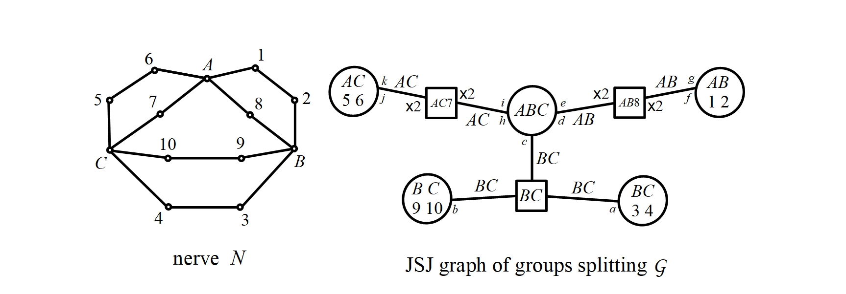
Figure 5.

There are no rigid vertices in $\mathcal{G}$, so there are also no rigid vertices in the corresponding Bass-Serre tree $T_{G}$. It follows then from Theorem B that the boundary $\partial G$ is a regular tree of $\theta$-graphs. Note that the defining graph $N$ clearly does not belong to the class $\mathcal{C}_{JS}$, so this examples goes beyond the class studied in an earlier mentioned paper [24]. (Obviously, it is easy to show many more examples of this sort, and another one, whose JSJ splitting contains a rigid factor, is described below in Example 14.6, see the group $G_{1}$ presented at Figure 6.) To get the explicit form of the regular tree of $\theta$-graphs homeomorphic to $\partial G$, i.e. to describe the corresponding graphical connecting system $\mathcal{R}_{G}$ as in Section 10, we need a closer analysis.

One deduces from the form of the graph of groups $\mathcal{G}$ that preimages in $T_{G}$ of the vertices $\langle A,B,8\rangle$ and $\langle A,C,7\rangle$ have degree 4, so that for any such preimage vertex $v$ there are precisely two edges issuing from $v$ that are mapped to each edge issuing from $\langle A,B,8\rangle$ or $\langle A,C,7\rangle$ (this is indicated at Figure 5 by little symbols ”$\times 2$”). Preimages in $T_{G}$ of the vertex $\langle B,C\rangle$ have degree 3. Each of the 2-ended groups at vertices of type (v2) is non-orientable, because it is either an infinite dihedral group, or the product of an infinite dihedral group with a group of order 2. It follows that all flexible factors of the Bowditch JSJ splitting of $G$ are also non-orientable.

According to our exposition in Section 10, the graphical connecting system $\mathcal{R}_{G}=(\Gamma,{\bf a},\mathcal{A})$ is described as follows. First, $\Gamma$ is the disjoint union of two copies of the $\theta$-graph $\Xi_{4}$ (corresponding to vertices $\langle A,B,8\rangle$ and $\langle A,C,7\rangle$), which we denote $\Gamma_{2}$ and $\Gamma_{3}$, respectively, and one copy of the $\theta$-graph $\Xi_{3}$ (corresponding to the vertex $\langle B,C\rangle$), which we denote $\Gamma_{1}$. The $V$-involution ${\bf a}$ of $\mathcal{R}_{G}$ is just the union of the standard $V$-involutions (as described in Example 7.11) for the $\theta$-graphs $\Gamma_{1}$, $\Gamma_{2}$ and $\Gamma_{3}$.

To describe the set $\mathcal{A}$ of $E$-connections for $\Gamma$, denote by $a,b,c$ the edges of $\Gamma_{1}$, by $d,e,f,g$ the edges of $\Gamma_{2}$, and by $h,i,j,k$ the edges of $\Gamma_{3}$, and for each of those edges fix one of its orientations (so that these letters actually denote oriented edges). According to the description in Section 10, for each $\Gamma_{i}$ we fix a bijection between the set of edges of $\Gamma_{i}$ and the set of vertices in $T_{G}$ adjacent to the vertex $z\in Z$ representing this component. We have indicated our choices of these bijections by assigning letters $a,\dots,k$ to flexible vertices of the graph in the right part of Figure 5. Any set $Y$ of representatives of flexible vertices in $T_{G}$ can be canonically identified with the set of vertices represented by circles at Figure 5. It follows that the sets $E_{y}:y\in Y$ coincide with the sets $\{a\}$, $\{b\}$, $\{c,d,e,h,i\}$, $\{f,g\}$ and $\{j,k\}$. Due to non-orientability of all flexible factors, the set of $E$-connections has then the form

$$\mathcal{A}=\bigcup_{y\in Y}E_{y}^{\pm}\times E_{y}^{\pm},$$

with $E_{y}:y\in Y$ as mentioned above.

Example 14.6.

Let $G_{1}=W_{N_{1}}$ and $G_{2}=W_{N_{2}}$ be the 1-ended hyperbolic RACG’s for the defining graphs $N_{i}$ as presented at the left parts of Figures 6 and 7, respectively. The central parts of these figures present the graph of groups decompositions $\mathcal{G}_{i}$ of these groups related to their Bowditch JSJ splittings. These decompositions have been obtained by referring to the results in [8]. Both underlying graphs $X_{i}$ of $\mathcal{G}_{i}$ contain a single vertex related to a rigid factor, namely the vertex represented by a hexagonal symbol, which corresponds to the special subgroup $H=\langle A,B,C,D\rangle<G_{i}$ in each of the two cases. It is also not hard to deduce from the form of $\mathcal{G}_{i}$’s that the corresponding rigid vertices in the Bass-Serre trees $T_{G_{i}}$ are not isolated, i.e they have some rigid neighbours at combinatorial distance 2. Thus, in both cases we have nontrivial rigid clusters, and we have rigid cluster factors which contain rigid factors as proper subgroups.

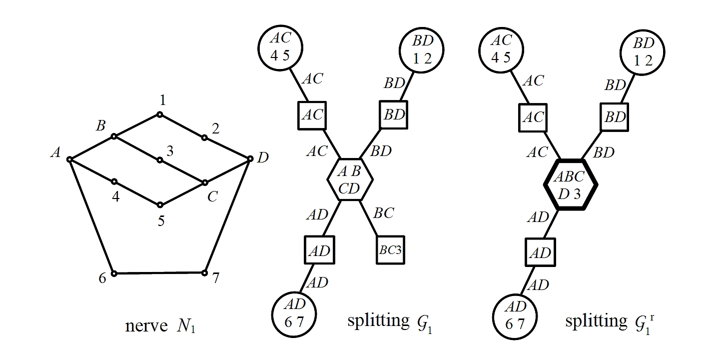
Figure 6.

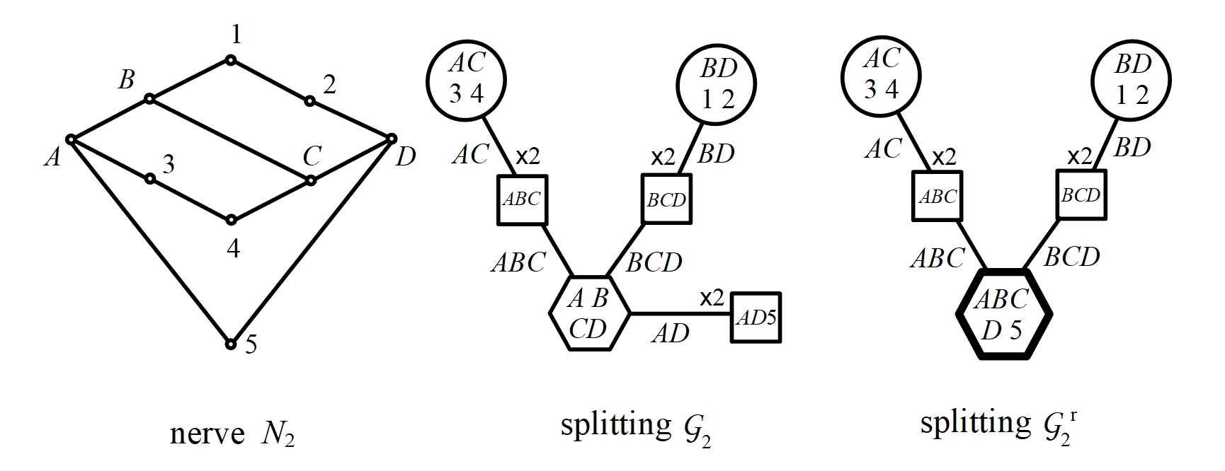
Figure 7.

Consider the graph of groups decompositions $\mathcal{G}^{r}_{i}$ of the groups $G_{i}$ related to their reduced Bowditch JSJ splittings. It is not hard to realize that they have forms as presented at the right parts of Figures 6 and 7. The rigid cluster factors correspond to the vertices indicated by the symbols of the bold hexagons. The rigid cluster factors in the group $G_{1}$ are the conjugates of the special subgroup $H_{1}=\langle A,B,C,D,3\rangle$, and it is not hard to see that they are virtually free. It follows then from Theorem A that the Gromov boundary $\partial G_{1}$ is a regular tree of 2-connected graphs. The explicit form of this tree of graphs, i.e. the corresponding graphical connecting system $\mathcal{R}_{G_{1}}$, can be extracted from the data in $\mathcal{G}^{r}_{1}$, and the least obvious, though still starightforward part of this extraction is the determination of the Whitehead graph associated to the rigid cluster factor $H_{1}$. We skip the details.

On the other hand, the rigid cluster factors in the group $G_{2}$ are the conjugates of the special subgroup $H_{2}=\langle A,B,C,D,5\rangle$ (see Figure 7). Since the defining graph of this subgroup is a 5-cycle, it is a cocompact Fuchsian group (it can be realized e.g. as the group generated by reflections in the sides of a right angled hyperbolic pentagon). The Gromov boundary of this subgroup is a circle, so the subgroup is not virtually free, even though the rigid factors from which it is formed are virtually free. It follows then from Theorem A that the Gromov boundary $\partial G_{2}$ is not homeomorphic to any tree of graphs.

References

- [1] B. H. Bowditch. Cut points and canonical splittings of hyperbolic groups. Acta Math., 180(2):145–186, 1998.
- [2] B. H. Bowditch. Relatively hyperbolic groups. Internat. J. Algebra Comput., 22(3):1250016, 66, 2012.
- [3] M. Brown. Some applications of an approximation theorem for inverse limits. Proc. Amer. Math. Soc., 11:478–483, 1960.
- [4] C. H. Cashen. Splitting line patterns in free groups. Algebr. Geom. Topol., 16(2):621–673, 2016.
- [5] C. H. Cashen. A geometric proof of the structure theorem for cyclic splittings of free groups. Topology Proc., 50:335–349, 2017.
- [6] C. H. Cashen and A. Martin. Quasi-isometries between groups with two-ended splittings. Math. Proc. Cambridge Philos. Soc., 162(2):249–291, 2017.
- [7] F. Dahmani and N. Touikan. Deciding isomorphy using Dehn fillings, the splitting case. Invent. Math., 215(1):81–169, 2019.
- [8] P. Dani and A. Thomas. Bowditch’s JSJ tree and the quasi-isometry classification of certain Coxeter groups. J. Topol., 10(4):1066–1106, 2017.
- [9] R. J. Daverman. Decompositions of manifolds, volume 124 of Pure and Applied Mathematics. Academic Press, Inc., Orlando, FL, 1986.
- [10] M. W. Davis. The geometry and topology of Coxeter groups, volume 32 of London Mathematical Society Monographs Series. Princeton University Press, Princeton, NJ, 2008.
- [11] A. N. Dranishnikov. Cohomological dimension of Markov compacta. Topology Appl., 154(7):1341–1358, 2007.
- [12] M. J. Dunwoody. The accessibility of finitely presented groups. Invent. Math., 81(3):449–457, 1985.
- [13] M. J. Dunwoody and M. E. Sageev. JSJ-splittings for finitely presented groups over slender groups. Invent. Math., 135(1):25–44, 1999.
- [14] I. Kapovich and N. Benakli. Boundaries of hyperbolic groups. In Combinatorial and geometric group theory (New York, 2000/Hoboken, NJ, 2001), volume 296 of Contemp. Math., pages 39–93. Amer. Math. Soc., Providence, RI, 2002.
- [15] S.-h. Kim and G. Walsh. Some groups with planar boundaries. In Surveys in differential geometry 2020. Surveys in 3-manifold topology and geometry, volume 25 of Surv. Differ. Geom., pages 253–280. Int. Press, Boston, MA, [2022] ©2022.
- [16] A. Martin. Non-positively curved complexes of groups and boundaries. Geom. Topol., 18(1):31–102, 2014.
- [17] J. W. Morgan and P. B. Shalen. Valuations, trees, and degenerations of hyperbolic structures. I. Ann. of Math. (2), 120(3):401–476, 1984.
- [18] D. Pawlik. Gromov boundaries as markov compacta. Preprint, arXiv:1503.04577, 2015.
- [19] D. Pawlik and A. Zabłocki. Trees of multidisks as gromov boundaries of amalgamated products. Preprint, arXiv:1602.00335v1, 2016.
- [20] J.-P. Serre. Trees. Springer Monographs in Mathematics. Springer-Verlag, Berlin, 2003. Translated from the French original by John Stillwell, Corrected 2nd printing of the 1980 English translation.
- [21] E. L. Swenson. Quasi-convex groups of isometries of negatively curved spaces. Topology and its Applications, 110(1):119–129, 2001.
- [22] J. Świa̧tkowski. The dense amalgam of metric compacta and topological characterization of boundaries of free products of groups. Groups Geom. Dyn., 10(1):407–471, 2016.
- [23] J. Świa̧tkowski. Trees of metric compacta and trees of manifolds. Geom. Topol., 24(2):533–592, 2020.
- [24] J. Świa̧tkowski. Reflection trees of graphs as boundaries of Coxeter groups. Algebr. Geom. Topol., 21(1):351–420, 2021.
- [25] H. C. Tran. Relations between various boundaries of relatively hyperbolic groups. Internat. J. Algebra Comput., 23(7):1551–1572, 2013.