Contrastive Learning-Based Framework for Sim-to-Real Mapping of Lidar Point Clouds in Autonomous Driving Systems

Abstract

Perception sensor models are essential elements of automotive simulation environments; they also serve as powerful tools for creating synthetic datasets to train deep learning-based perception models. Developing realistic perception sensor models poses a significant challenge due to the large gap between simulated sensor data and real-world sensor outputs, known as the sim-to-real gap. To address this problem, learning-based models have emerged as promising solutions in recent years, with unparalleled potential to map low-fidelity simulated sensor data into highly realistic outputs. Motivated by this potential, this paper focuses on sim-to-real mapping of Lidar point clouds, a widely used perception sensor in automated driving systems. We introduce a novel Contrastive-Learning-based Sim-to-Real mapping framework, namely CLS2R, inspired by the recent advancements in image-to-image translation techniques. The proposed CLS2R framework employs a lossless representation of Lidar point clouds, considering all essential Lidar attributes such as depth, reflectance, and raydrop. We extensively evaluate the proposed framework, comparing it with the state-of-the-art image-to-image translation methods using a diverse range of metrics to assess realness, faithfulness, and the impact on the performance of a downstream task. Our results show that CLS2R demonstrates superior performance across nearly all metrics. Source code is available at https://github.com/hamedhaghighi/CLS2R.git.

I Introduction

Virtual verification and validation of Automated Driving Systems (ADS) is becoming an increasingly important part of their safety assurance frameworks primarily due to the safety concerns and high costs of extensive real-world testing [1]. Successful virtual verification and validation of ADS requires realistic simulation models including perception sensor models. In addition, perception sensor models are powerful tools for generating datasets that can be used to train deep learning-based perception models [2]. Motivated by these important needs, this paper aims to develop a realistic Lidar model, a key perception sensor in ADS [3].

The use of sensor models and the synthetic datasets they generate introduces the non-trivial technical challenge of closing the so-called sim-to-real gap [4]. This gap arises from inaccuracies in modelling 3D assets and perception sensors, resulting in a mismatch between the fidelity of simulated and real sensor data. Such discrepancies can undermine the reliability of the simulation for safety assurance and synthetic dataset generation for training of perception models.

The complexity of developing high-fidelity sensor models has led to the growing popularity of learning-based models to bridge the sim-to-real gap [5, 6]. In the context of Lidar models, most existing learning-based approaches aim to design deep neural networks for learning complex Lidar data attributes. These models acquire knowledge from real-world data, and this knowledge is then transferred to simulation environments. For instance, Vacek et al. [7] attempted to learn Lidar reflectance from the real recorded KITTI [8], and then, they deployed their model within the CARLA [9] simulation environment. Despite exhibiting promising results, these approaches often focus only on specific Lidar attributes, such as reflectance and raydrop, and rely on conventional simulation techniques for the other aspects. This has led to another set of methods[10] in the literature that attempt to establish a direct mapping between simulation and real, commonly known as sim-to-real domain mapping methods. In the context of the Lidar data, existing sim-to-real mapping approaches mainly use vanilla CycleGAN [11] to map the lossy Birds-Eye-View (BEV) representation of the point clouds. These approaches are primarily leveraged for training downstream perception models. However, the effectiveness of such approaches from the perspective of realness and faithfulness has not been fully analysed in the literature.

Inspired by the success of contrastive learning in unpaired image-to-image translation methods [12], we propose a novel framework for sim-to-real mapping of Lidar point clouds. We term this method Contrastive-Learning-based Sim-to-Real mapping (CLS2R). The proposed CLS2R uses a lossless representation of Lidar point clouds and undergoes a comprehensive evaluation using a diverse set of metrics extending beyond the scope of current research in the field. The CLS2R framework is the first of its type to model all essential Lidar data attributes, including depth, reflectance and raydrop based on the corresponding simulated data. Inspired by the noise rendering in Convolutional Neural Networks (CNNs) [13], we disentangle the synthesis of raydrop from the synthesis of depth-reflectance image, employing a reparametrisation trick [14] to fuse them effectively. CLS2R also incorporates auxiliary images, e.g. point-wise semantic labels, using a unique strategy to improve the overall quality of the simulated Lidar point clouds.

To evaluate the performance of the proposed CLS2R framework, we created a synthetic dataset of point-wise annotated Lidar point clouds and RGB camera images using the CARLA simulator, named semantic-CARLA. We assess the proposed CLS2R extensively from the perspective of realness, faithfulness, and effectiveness on a downstream perception task. The results show that CLS2R outperforms state-of-the-art methods measured by key qualitative and quantitative performance indicators such as FID [15]. The following bullet points outline the summary of the contributions of this paper:

• A novel framework, namely CLS2R, proposed for sim-to-real domain mapping of Lidar point clouds. The proposed CLS2R outperforms the state-of-the-art image-to-image translation techniques across almost all evaluation metrics.

• A new publicly accessible dataset consisting of synthetic, point-wise annotated Lidar point clouds and RGB images of driving scenes generated for future studies of the subject by the interested research community.

• A comprehensive evaluation of the CLS2R model in terms of realness, faithfulness, and the performance of a downstream perception model.

II Related-Work

This section provides an overview of the related works in the literature, including learning-based Lidar modelling approaches and synthetic Lidar datasets.

II-A Learning-based Lidar Models

Learning-based Lidar models have recently gained popularity as a preferred alternative to high-fidelity physics-based models because of their capacity to discover intricate patterns in data. We divide these models into two categories: those focused on ‘Learning from Real Domain’ and those adopting the ‘Sim-to-Real Domain Mapping’ approach.

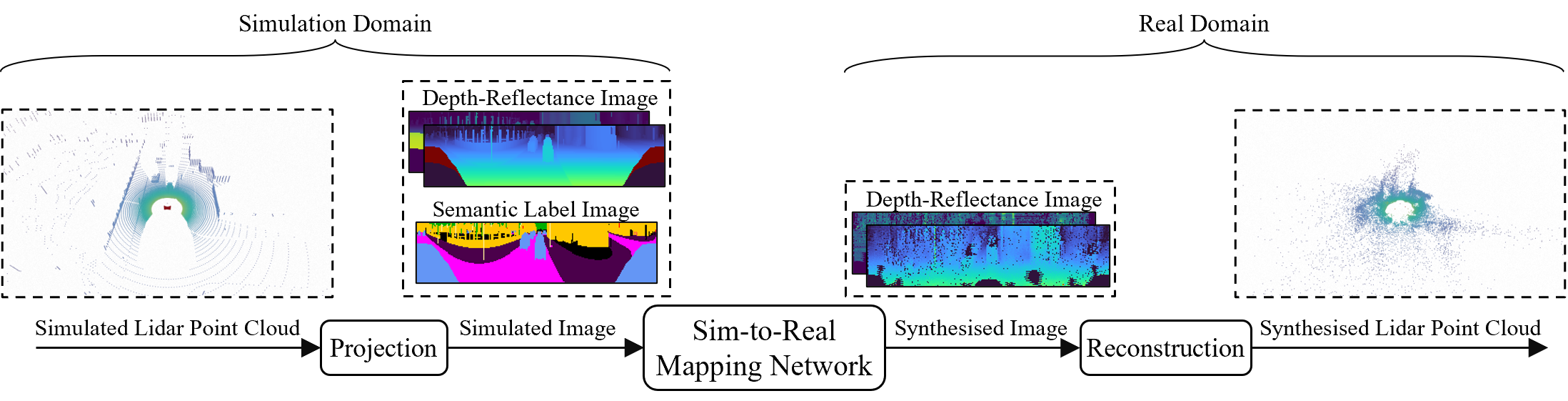
Figure 1: Overview of the proposed CLS2R framework.

Regarding the first category, several works have conditioned easy-to-simulate Lidar data attributes, e.g. depth, to predict more complex ones, e.g. reflectance and raydrop. For instance, Vacek et al. [7] and Wu et al. [16] used neural networks to predict Lidar reflectance based on other modalities, e.g. spatial coordinates. Similarly, Guillard et al. [17], Zhao et al. [18], and [19] attempted to estimate Lidar raydrop using data-driven techniques. While the aforementioned methods demonstrate promising results, they are restricted in the sense that they focus on learning specific attributes, relying on traditional simulation algorithms for other aspects.

To close the sim-to-real gap, the second category of methods aims to find a direct mapping between simulation and real. Since the real and simulated data are usually unpaired, the problem can be formulated as finding an unpaired data mapping. Due to the outstanding performance of CycleGAN [11] in unpaired image-to-image translation, several works have adopted this framework for Lidar point cloud translation. For example, Sallab et al. [20] and Saleh et al. [10] have converted Lidar point clouds to BEV range images and used CycleGAN for transformation. Both works evaluated their methods using domain adaptation for object detection, demonstrating improved performance while using the synthesised images. Despite their great success, the synthesised BEV images cannot be reverted to 3D point clouds as the transformation is non-bijective. Moreover, these techniques have been evaluated through downstream tasks such as object detection without thorough analysis from the perspective of synthesis realism, and faithfulness.

The proposed CLS2R in this paper can be classed as a sim-to-real domain mapping approach inspired by image-to-image translation models. However, we use a lossless representation of the Lidar point cloud based on polar coordinates. Moreover, our framework can synthesise various data attributes such as depth, reflectance, and raydrop images.

II-B Synthetic Lidar Datasets

Several synthetic driving datasets tailored for training ADS perception models have recently been released. However, only a few of these contain Lidar data with different auxiliary data consisting of point-wise semantic labels, RGB colour, and reflectance. Among these, Presil [21] stands as one of the pioneering datasets using the GTA-V graphics engine to ray-cast Lidar point clouds. While this dataset contains RGB images and point-wise semantic labels, the classes are only limited to ‘Car’ and ‘Person’ due to the constraints of the GTA-V simulation environment. On the other hand, the more recent datasets, such as SHIFT [2] and AIOD [22], include comprehensive sensor suits, including different levels of annotations. While the SHIFT [2] dataset focuses mainly on capturing various discrete and continuous domains in real-world driving, AIOD covers out-of-distribution scenarios and long-range perception. Although the aforementioned datasets mainly focus on providing larger datasets containing more driving conditions, our proposed dataset is mainly created for the sim-to-real mapping task, as we explain in Section V-A1.

III Problem Formulation

Sim-to-real mapping problem can be formulated as finding a function, denoted by $G:\mathcal{P_{X}}\rightarrow\mathcal{P_{Y}}$, that transforms Lidar point clouds from simulation domain $\mathcal{P_{X}}\subset\mathbb{R}^{N\times(4+M)}$ into real domain $\mathcal{P_{Y}}\subset\mathbb{R}^{N\times 4}$. This is given the corresponding simulated $P_{X}=\{p_{x}\in\mathcal{P_{X}}\}$ and real datasets $P_{Y}=\{p_{y}\in\mathcal{P_{Y}}\}$. In this formulation, simulated Lidar point cloud $p_{x}$ consists of $N$ points with four plus $M$ dimensions. The initial four dimensions include three dimensions for 3D spatial coordinates and one for reflectance; While additional M dimensions contain auxiliary data such as point-wise semantic labels or RGB colours. Real Lidar point cloud $p_{y}$ contains N points with four dimensions (for 3D coordinates and reflectance). As detailed in Section IV-A, we project the Lidar point clouds into images of dimensions $H\times W$. Using this data representation, the problem formulation is transformed into an equivalent of finding a mapping $G$ between the projected Lidar point clouds from simulation $\mathcal{X}\subset\mathbb{R}^{H\times W\times(2+M)}$ and real domain $\mathcal{Y}\subset\mathbb{R}^{H\times W\times 2}$. This is given the corresponding simulated $X=\{x\in\mathcal{X}\}$ and real dataset $Y=\{y\in\mathcal{Y}\}$.

IV CLS2R Framework

The overview of the proposed CLS2R framework is depicted in Fig. 1. We first project the simulated Lidar point clouds, into depth-reflectance images and semantic label images. These images are then mapped into highly realistic depth-reflectance images through a sim-to-real mapping network. Finally, the output of the mapping network is converted back into realistic Lidar point clouds through a reconstruction transformation. The details of the components, as well as the training process of the CLS2R framework are discussed in the following subsections.

IV-A Point Cloud Projection and Reconstruction

To leverage the power of CNN-based networks for sim-to-real mapping in the proposed framework, we convert the Lidar point clouds into image-based representation via a lossless projection. Considering $H,W$ as the vertical and horizontal angular resolution of mechanical rotating Lidar, we create an image of $H\times W$ dimension, assigning each point a pixel based on its azimuth and elevation angle $(\theta,\phi)$. Point-wise depth, reflectance, and M auxiliary attributes are stored in the assigned pixel. Therefore, the original point cloud array with a shape of $N\times(4+M)$ is transformed into an image array with a shape of $H\times W\times(2+M)$ using this projection. The angles $(\theta,\phi)$ can be calculated using 3D spatial coordinates $(x,y,z)$ of point cloud as:

$$(\theta,\phi)=(\arctan 2(y,x),\arctan 2(z,\sqrt{x^{2}+y^{2}})).$$ (1)

Similarly, we reconstruct the output depth-reflectance image array with a shape of $H\times W\times 2$ back to the point cloud array with a shape of $N\times 4$ in a lossless manner. The reconstruction utilises the azimuth and elevation angle $(\theta,\phi)$ of each pixel, along with the corresponding depth $d$, to restore the $(x,y,z)$ as:

$$(x,y,z)=(d\cos(\phi)\cos(\theta),d\cos(\phi)\sin(\theta),d\sin(\phi)).$$ (2)

IV-B Sim-to-Real Mapping Network

Inspired by the recently developed image-to-image translation networks [23], our sim-to-real mapping network $G$ adopts an encoder-decoder architecture, as shown in Fig. 2. The inference flow of $G$ entails encoding the simulated images $x$ with $G_{enc}$ and $E$, decoding the latent vector with $G_{dec}$, and then using Raydrop Synthesis (RS) to synthesise the output $\hat{y}$. Since we needed to use $G_{enc}$ to extract features from both $x$ and $\hat{y}$ for the PatchNCE loss (see Section IV-C for more details), and these inputs may not necessarily have similar tensor shapes, we decouple the encoding of $x\in\mathbb{R}^{H\times W\times 3}$ into the encoding of depth-reflectance image $d\in\mathbb{R}^{H\times W\times 2}$ and the encoding of the semantic label image $c\in\mathbb{R}^{H\times W\times 1}$.

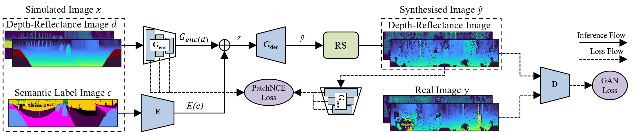
Figure 2: Overview of the inference and training losses of our sim-to-real mapping network $G$. The network consists of $G_{enc}$, $E$, and $G_{dec}$ sub-networks. $G_{enc}$ encodes depth-reflectance image $d$ and $E$ encodes auxiliary image $c$. These two codes are summed up to form $z$ which are then decoded by $G_{dec}$ to output $\tilde{y}$. The Raydrop Synthesis (RS) module renders raydrop and synthesises the final image $\hat{y}$. The network is trained with GAN loss [24] using the discriminator $D$, and PatchNCE loss [12] using the features extracted by $G_{enc}$.

In this design, $G_{enc}$ and $E$ encodes $d$ and $c$ respectively and form latent vector $z=G_{enc}(d)+E(c)$. $z$ is decoded to $\tilde{y}$ using $G_{dec}$, and finally, $\tilde{y}$ is converted to $\hat{y}$ using the RS component. The mapping process can be calculated as:

$$\begin{split}\hat{y}&=G(x)=RS(\tilde{y})=RS(G_{dec}(z))\\ &=RS(G_{dec}(G_{enc}(d)+E(c))).\end{split}$$ (3)

As shown in Fig. 3, the RS component renders raydrop patterns, i.e. missing transmitted rays, on the synthesised depth-reflectance image $\tilde{y}$, Raydrop happens when the ray travel distance surpasses the maximum detection range or when it hits refractive or highly reflective surfaces. Concerning the image-based representation of the Lidar point cloud, raydrop can be represented as a binary mask. While ray-drop mask can be implicitly synthesised by our generator, CNNs commonly encounter difficulty in modelling noise in images [13]. Therefore, we disentangle the synthesis of Lidar scans into modelling complete scans (without the missed information) and the ray-drop mask. We first generate $\tilde{y}\in\mathbb{R}^{H\times W\times 3}$ , which is a concatenation of complete depth-reflectance images $\tilde{y}_{l}\in\mathbb{R}^{H\times W\times 2}$ and a raydrop logits image $\tilde{y}_{p}\in\mathbb{R}^{H\times W\times 1}$. We then obtain ray-drop mask $\tilde{y}_{m}$ by sampling from a Bernoulli distribution with $\tilde{y}_{p}$ as the parameter:

$$\begin{split}\tilde{y}_{m}\sim Bernoulli(\tilde{y}_{p}),\end{split}$$ (4)

where $y_{m}$ is a binary mask indicating which points to keep and which to drop. Using the mask, $\hat{y}$ is calculated by multiplying the mask into the complete scans as $\hat{y}=\tilde{y}_{m}\odot\tilde{y}_{l}$. Since sampling from the Bernoulli distribution is not a differentiable operation, we use the re-parametrisation trick to estimate the gradient in the backpropagation. We re-parameterise $\tilde{y}_{m}$ with a continuous relaxation $y^{\prime}_{m}$ using Gumbel-Sigmoid distribution [14] as:

$$\begin{split}y^{\prime}_{m}=sigmoid\bigg{(}\frac{(\log(\tilde{y}_{p})+g_{1})-(\log(1-\tilde{y}_{p})+g_{2})}{\alpha}\bigg{)},\end{split}$$ (5)

where $g_{1}\in R^{H\times W}$ and $g_{2}\in R^{H\times W}$ are two i.d.d samples for from $Gumbel(0,I)$ making the process random. Furthermore, $\alpha$ controls the gap between the relaxed and original Bernoulli distribution. The re-parameterised sample $y^{\prime}_{m}$ is then discretised to binary mask by being thresholded against $0.5$. This can be written as:

$$\tilde{y}_{m}=\begin{cases}1&y^{\prime}_{m}\geq 0.5\\ 0&y^{\prime}_{m}<0.5.\end{cases}$$ (6)

The thresholding is only used for the forward pass of the network and is replaced with the identity function in order to enable gradient propagation.

IV-C Training

As shown in Fig. 2 (Loss Flow), we train our network G using GAN [24] and PatchNCE[12] losses. To synthesise realistic data, the output of the mapping $G$ should be indistinguishable from that of real domain data $y$. To this end, we leverage the GAN loss, involving the simultaneous optimisation of two networks, the generator $G$ (equivalent to our mapping function) and the discriminator $D$, in a competitive setting. The network $G$ attempts to generate realistic data which is indistinguishable by $D$, and $D$ aims to differentiate $G$’s output from real inputs. The GAN loss can be calculated as:

$$\begin{split}\mathcal{L}_{GAN}(G,D,X,Y)=&\mathbb{E}_{y\sim Y}[\log D(y)]\\ +&\mathbb{E}_{x\sim X}[\log(1-D(G(x))].\\ \end{split}$$ (7)

If the training of G relies solely on minimising the GAN loss, the mapping might learn to generate data that is realistic enough to fool the discriminator irrespective of the input. To avoid this problem and to assure that the content of the input is accurately translated, CLS2R uses PatchNCE loss [12]. PatchNCE enforces consistency between input and output images using contrastive learning. Via this technique, the generator learns to synthesise images such that input-output patches at the same spatial location are given the highest similarity compared with patches at the other locations. For example, an output image patch containing a car matches more closely with the input patch containing a car than with a patch containing a pedestrian. To extract patch-wise information, we use the features already extracted in the encoding layers of the $G$, denoted as $G_{enc}$, and post-process it via a Multi-Layer-Perceptron (MLP) $H$. For an $L$ layer $G_{enc}$, the features in the layer $l$ can be described as $\{z_{l}\}_{l=1}^{L}=\{H_{l}(G^{l}_{enc}(x))\}_{l=1}^{L}$ for the input images and $\{\hat{z}_{l}\}_{l=1}^{L}=\{H_{l}(G^{l}_{enc}(\hat{y})\}_{l=1}^{L}$ for the output images. Each spatial location $u\in\{1,\ ...,\ U_{l}\}$ of $z_{l}$ contains features of an input patch and the higher the encoding layer $l$ is, the larger patch it captures. We refer to $u^{th}$ location of $z_{l}$ as $z_{l}^{u}\in\mathbb{R}^{C_{l}}$ and other locations as $z_{l}^{U\backslash u}\in\mathbb{R}^{C_{l}}$, where $C_{l}$ is the number of channels at each layer. Similar to PatchNCE, we use cosine similarity to establish the correspondence between $\hat{z_{l}^{u}}$ and $z_{l}^{u}$ as:

$$\begin{split}&l(\hat{z}_{l}^{u},z_{l}^{u},z_{l}^{U\backslash u})=\\ -&\log{\Bigg{[}\frac{\exp{(\hat{z}_{l}^{u}\cdot z_{l}^{u}/\tau)}}{\exp{(\hat{z}_{l}^{u}\cdot z_{l}^{u}/\tau)}+\sum_{s\in U\backslash u}\exp(\hat{z}_{l}^{u}\cdot z_{l}^{s}/\tau)}\Bigg{]}},\end{split}$$ (8)

where $\tau=0.07$ is the temperature to scale the distances. Using the Equation 8, the PatchNCE loss can be written as:

$$\mathcal{L}_{patchNCE}(G,H,X)=\mathbb{E}_{x\sim X}\sum_{l=1}^{L}\sum_{u=1}^{U_{l}}(\hat{z}_{l}^{u},z_{l}^{u},z_{l}^{U\backslash u}).$$ (9)

We also include PatchNCE loss on the real domain $\mathcal{Y}$, referred to as $\mathcal{L}_{patchNCE}(G,H,Y)$, to ensure that the network does not change the realistic input images. The overall objective $\mathcal{L}$ can be calculated as:

$$\begin{split}\mathcal{L}=\mathcal{L}_{GAN}(G,D,X,Y)&+\lambda_{nce}\mathcal{L}_{PatchNCE}(G,H,X)\\ &+\lambda_{idt}\mathcal{L}_{PatchNCE}(G,H,Y).\end{split}$$ (10)

The hyperparameters $\lambda_{idt}$ and $\lambda_{nce}$ balance the emphasis between the reconstruction error (faithfulness) in the mapping process and the proximity to the real distribution (realness) in the GAN loss.

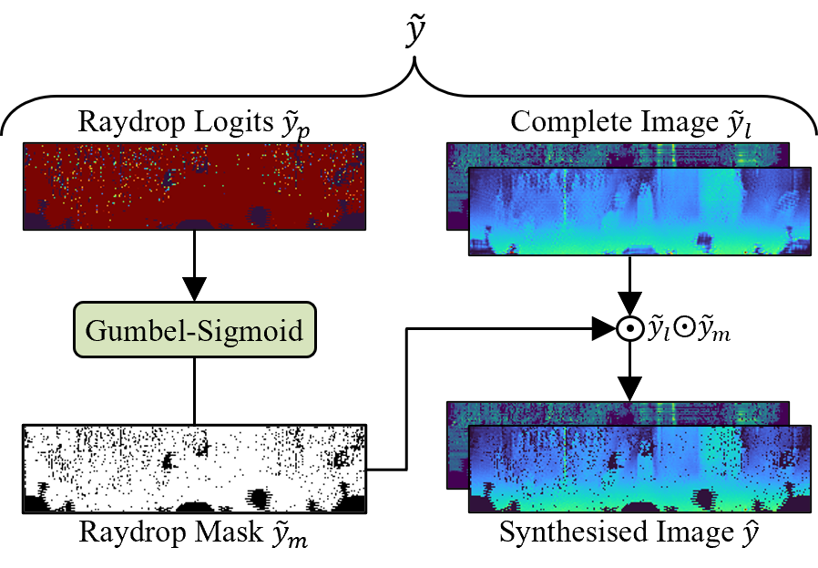
Figure 3: Overview of Raydrop Synthesis (RS) Module. The RS module inputs $\tilde{y}$ consisting of raydrop logits $\tilde{y}_{p}$ and complete depth-reflectance image $\tilde{y}_{l}$. We use $\tilde{y}_{p}$ as the parameter of Bernoulli distribution and sample from the distribution using the Gumbel-Sigmoid [14] function to yield raydrop mask $\tilde{y}_{m}$. The raydrop mask is then multiplied with the complete image, resulting in the final synthesised image $\hat{y}$.

TABLE I: Quantitative comparison to stat-of-the-art methods. The best results are bolded, and the second-best results are underlined. $\downarrow$: The lower, the better. $\uparrow$: The higher, the better.

Dataset	Method∗	FID $\downarrow$	SWD $\downarrow$	JSD $\downarrow$	MMD $\times 10\downarrow$	CD $\times 10\downarrow$	RMSE $\downarrow$	PixelAcc $\uparrow$
Semantic-KITTI	Semantic-CARLA	2980	2.35	0.254	0.14	-	-	0.41
	U-Net [25]	2601	1.11	0.159	0.04	0.037	0.380	0.63
	CycleGAN[11]	2052	0.54	0.100	0.08	0.037	0.378	0.56
	GcGAN [26]	2458	0.46	0.475	0.73	0.225	0.409	0.53
	CLS2R (Ours)	1851	0.45	0.071	0.03	0.032	0.376	0.57
	Training Set	1318	0.31	0.013	0.02	-	-	0.77
SemanticPOSS	Semantic-CARLA	4819	2.09	0.51	0.24	-	-	0.20
	U-Net[25]	4019	1.33	0.27	0.06	0.070	0.258	0.32
	CycleGAN[11]	3775	1.06	0.36	0.45	0.066	0.502	0.25
	GcGAN[26]	3522	1.52	0.41	0.38	0.114	0.347	0.27
	CLS2R (Ours)	3365	0.59	0.23	0.09	0.063	0.217	0.29
	Training Set	2848	0.75	0.06	0.04	-	-	0.61
∗It is important to note that we add the Raydrop Synthesis (RS) module to all state-of-the-art models for a fair comparison.

V Evaluations

This section describes the evaluations of the proposed CLS2R framework. First, we explain the experimental settings, followed by a detailed explanation of the evaluations, which includes a comparison to the state-of-the-art methods, studying the impact on a downstream perception task, and performing an ablation study.

V-A Experimental Settings

This subsection describes the datasets, evaluation metrics used in our study as well as implementation details of the experiments.

V-A1 Datasets

The training of the CLS2R requires datasets from both the simulation and real domains to find the underlying mapping function. Regarding the simulated Lidar point clouds, we created our dataset, which we term semantic-CARLA. We specifically structured the semantic-CARLA dataset to have similar scene objects, sensor configuration and data format as the semantic-KITTI [27] dataset. This design choice aims to minimise the sim-to-real gap, enabling CLS2R to focus only on identifying sensor-related phenomena. We selected the semantic-KITTI dataset as our real reference due to its broad use in autonomous driving research that has incited the creation of subsequent driving datasets.

To create semantic-CARLA, we used the CARLA [9] simulation tool and replicated the configuration of Lidar and RGB camera sensors to match the original setup of the KITTI [8] dataset. Specifically, we simulated a 10 frame-per-second (fps) Velodyne HDL-64E Lidar, producing approximately 100K points in each rotation, along with a 10 fps RGB camera with $1241\times 376$ image resolution. We also recorded point-wise semantic labels of Lidar point clouds classifying points into sixteen different classes. The entire dataset consists of approximately 34k scans collected in 8 different CARLA environments.

Concerning the real datasets, we picked the commonly used Lidar datasets of Semantic-KITTI [28] and semantic-POSS [29]. Semantic-KITTI is a point-wised labelled version of the original KITTI’s visual odometry benchmark. The dataset consists of 22 sequences of Lidar (Velodyne HDL-64E) scans, from which 11 sequences (approximately 19k scans) have publicly available annotations. Semantic-POSS have the same data format as semantic-KITTI and contains 3k complex Lidar scans collected at Peking University. We designated sequences 7 and 8 from the semantic-KITT, as well as sequences 4 and 5 from SemanticPOSS for validation and testing respectively.

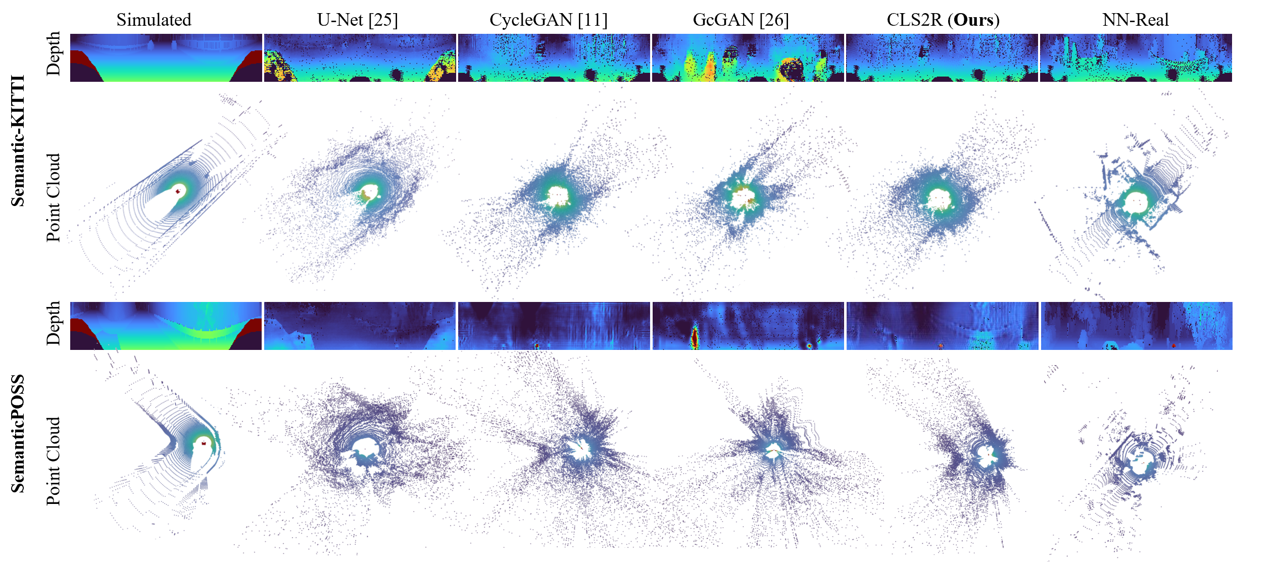
Figure 4: Qualitative comparison to state-of-the-art methods. Each column demonstrates different methods, and each row shows synthesised depth images and the reconstructed point clouds in the specified dataset. ‘Simulated’ and ‘NN-Real’ columns exhibit the simulated input data and nearest neighbour sample in the real dataset, respectively.

V-A2 Metrics

We assess the CLS2R framework and compare it to other established methods in terms of faithfulness and realness, considering both image-based and point cloud representations of the synthesised data. Additionally, we evaluate through a downstream perception task, specifically semantic segmentation. The following paragraphs delve into each category of the metrics: realness, faithfulness, and evaluation by a downstream task.

Evaluating the realness of synthesised data typically involves assessing the closeness between the distributions of real and synthesised data. To construct the sets of real and synthesised samples, we randomly selected 5000 samples from the test sets of both real and synthesised datasets. We adopt the metrics used in unconditional Lidar point cloud synthesis [30, 31] and calculate Fréchet Inception Distance (FID) [15] and Sliced Wasserstein Distance (SWD) [32] for the image-based representation, along with Jensen Shannon Distance (JSD) and Minimum Matching Distance (MMD) for the point cloud representation.

To assess the faithfulness of the simulated Lidar data, we employ Root Mean Square Error (RMSE) to quantify the distance between input-output depth images. We also compute the Chamfer Distance (CD) for point cloud representation.

To evaluate from the perspective of a downstream module, we measure the performance of the Rangenet++ [33] model for the semantic segmentation task. We feed the pre-trained model with synthesised data and calculate the pixel-wise accuracy (PixelAcc). We also train the model with synthesised data and compute the precision, recall, and Intersection Over Union (IOU). The Rangenet++ model’s performance inherently indicates both the realism and faithfulness of the synthesised data.

V-A3 Implementation details

We follow the setting of [12] for contrastive learning and network architecture, with a few modifications. Specifically, we set $\lambda_{idt}=2$, $\lambda_{nce}=1$ in Equation 10 and $\alpha=1$ in Equation 5 due to the better faithfulness-realness trade-off and loss convergence. We use Adam optimiser with a learning rate of $5e^{-5}$ and implement linear learning rate decay of 0.5 at every 10th epoch. We set the batch size to 12 and observed training convergence at approximately 80 epochs. We implemented the networks using Pytorch Library and conducted all the experiments on NVIDIA Geforce RTX 3090 GPUs.

TABLE II: Results of Ablation Study. We incrementally incorporate Raydrop Synthesis (RS), Contrastive Learning (CL), and Auxiliary Images (AI) into our Baseline and examine the effects. $\downarrow$: The lower the better. $\uparrow$: The higher the better.

Dataset	Method	FID $\downarrow$	SWD $\downarrow$	JSD $\downarrow$	MMD $\times 10\downarrow$	CD $\times 10\downarrow$	RMSE $\downarrow$	PixelAcc $\uparrow$
Semantic-KITTI	Baseline	2939	1.76	0.434	0.52	0.063	0.508	0.48
	Baseline + RS	2052	0.54	0.103	0.08	0.037	0.378	0.56
	Baseline + RS + CL	1846	0.55	0.076	0.04	0.035	0.368	0.55
	Baseline + RS + CL + AI (CLS2R)	1851	0.45	0.071	0.03	0.032	0.376	0.57
SemanticPOSS	Baseline	4046	1.82	0.401	0.48	0.272	0.862	0.19
	Baseline + RS	3775	1.06	0.369	0.45	0.066	0.502	0.25
	Baseline + RS + CL	3282	0.79	0.240	0.10	0.089	0.238	0.28
	Baseline + RS + CL + AI (CLS2R)	3365	0.59	0.228	0.09	0.063	0.217	0.29

TABLE III: Evaluation through a downstream task performance. Following the previous works [7, 17], we report the performance of a semantic segmentation model, Rangenet++ [33], when it is trained by our synthesised data versus the simulated data (Semantic-CARLA) on the ‘Car’ class. The evaluation involves reporting precision, recall, and IOU, all represented as percentages.

Test Dataset	Training Dataset	Precision [%]	Recall [%]	IOU [%]
Semantic-KITTI	Semantic-CARLA	21.75	12.91	7.54
	Synthesised by CLS2R	29.85	31.03	16.56
SemanticPOSS	Semantic-CARLA	14.06	3.28	2.70
	Synthesised by CLS2R	32.91	16.50	12.57

V-B Comparison to State-of-the-Art Methods

Since the existing learning-based Lidar models do not generate all Lidar data attributes, and most of them are designed for BEV representation, we re-implement and adapt the state-of-the-art methods for a fair comparison. As discussed in Section II, several works [7, 16, 17, 19, 18] adopted U-Net [25] to learn Lidar data attributes, e.g. reflectance, from the real domain. As a representative of this group of methods, we trained U-Net-64 (consisting of 6 down-sampling and up-sampling layers) to predict the Lidar point clouds from the semantic segmentation layout on real data. We use L1 loss for training and refer to this framework as ‘U-Net’. Sim-to-real domain mapping frameworks [20, 10] use a CycleGAN [11] framework to map between synthetic and real BEV Lidar point clouds. We trained the framework on the image-based representation of Lidar point clouds and named this category of methods ‘CycleGAN’. Additionally, we train the state-of-the-art image-to-image translation method, Geometric-Consistent GAN (GcGAN) [26] framework, using a similar approach to CycleGAN. We integrate Gumbel-Sigmoid into all mentioned methods to synthesise raydrop as discussed in Section IV-B. As reported in Table I, our CLS2R attains the top performance in nearly all the metrics and the second best in the remaining one. CycleGAN and GcGAN achieve a comparable result to ours in terms of realness in image-based representation. This can be attributed to the presence of GAN loss, which pushes the images to have a real appearance. On the other hand, U-Net demonstrates comparable, or in some cases superior, performance in terms of realness in point cloud representation and overall faithfulness. We speculate that this may be attributed to the U-Net’s exclusive use of the L1 loss and its dependence solely on the semantic segmentation layout for the synthesis. It is also evident that our CLS2R has substantially enhanced the realism of simulated data (referred to as Semantic-CARLA) scans and has narrowed the gap compared to real data (referred to as ‘Training Set’).

We visualise the synthesised depth image of each method and the reconstructed point cloud in Fig 4. We also plot the simulated input data (indicated as ‘Simulated’) and the nearest neighbour real data corresponding to the synthesised depth images (indicated as ’NN-Real’). It can be seen that adversarial methods, including CycleGAN and GcGAN, exhibit hallucination artefacts by adding or removing objects from the scene. It is also apparent that the non-adversarial method, ‘U-Net’ does not yield a realistic appearance compared to ‘NN-Real’ samples. Conversely, our CLS2R is capable of synthesising a realistic Lidar point cloud while remaining faithful to the simulated data.

V-C Impact on Downstream Perception Model

To evaluate if our CLS2R can enhance the performance of a perception model by providing more realistic training datasets, we adopt the evaluation approach used in most learning-based Lidar models [7, 17]. In particular, we train a semantic segmentation model, Rangenet++ [33] in this instance, on the data synthesised by our CLS2R and report the performance using the precision, recall, and IOU metrics on the ‘Car’ class. These performance metrics are calculated on the test set of real data and are compared to the model’s performance when trained on the simulated data. As shown in Table III, our CLS2R demonstrates effectiveness in improving the performance, especially by reducing the false negatives, thus increasing the recall and IOU metrics.

V-D Ablation Study

We conduct an ablation study to investigate the impact of the proposed techniques in CLS2R on the performance. As a baseline model, we select the vanilla CycleGAN network [11] without the RS module. Our study encompasses three steps: firstly, the integration of RS into the baseline; secondly, replacing cycle-consistency with Contrastive Learning (CL), i.e. PatchNCE loss; and thirdly, the incorporation of Auxiliary Images (AI) into the input. As shown in Table II, adding RS to the baseline leads to a substantial increase in performance. This is because CNNs inherently filter high frequency in the images; Hence, disentangling the synthesis of the raydrop mask from Lidar scans can improve all the metrics significantly. Including CL in the second step significantly improves the realness metrics such as FID, JSD, and MMD, while most other metrics remain roughly unchanged. This improvement can be attributed to a more stringent consistency objective, PatchNCE, leading to a better solution. Regarding the third step, the incorporation of AI shows to have a 5-10% improvement in most of the metrics. It is worth mentioning that we did not observe significant improvement while using RGB images; therefore, the auxiliary images in all experiments only contained the semantic segmentation layout.

VI Conclusion

In this paper, we proposed a novel framework for sim-to-real mapping of Lidar point clouds using contrastive learning. As a part of this research, we also created a novel dataset, namely the Semantic-CARLA dataset. We assessed sim-to-real mapping performance using a multitude of metrics quantifying realness, faithfulness and performance of the downstream perception task. Our evaluations highlighted the significant impact of contrastive learning and the raydrop synthesis module on improving performance. Moreover, the results revealed that our CLS2R not only synthesises realistic data but also faithfully represents the simulation, achieving superior results across nearly all metrics compared to state-of-the-art methods. We hope this work inspires further research aimed at bridging the gap between simulation and real-world data, particularly on Lidar point clouds.

References

- [1] N. Kalra and S. Paddock, Driving to Safety: How Many Miles of Driving Would It Take to Demonstrate Autonomous Vehicle Reliability? RAND Corporation, 5 2016.
- [2] T. Sun, M. Segu, J. Postels, Y. Wang, L. Van Gool, B. Schiele, F. Tombari, and F. Yu, “SHIFT: a synthetic driving dataset for continuous multi-task domain adaptation,” in Computer Vision and Pattern Recognition, 2022.
- [3] F. Rosique, P. J. Navarro, C. Fernández, and A. Padilla, “A systematic review of perception system and simulators for autonomous vehicles research,” Sensors, vol. 19, no. 3, 2019. [Online]. Available: https://www.mdpi.com/1424-8220/19/3/648
- [4] A. Kadian, J. Truong, A. Gokaslan, A. Clegg, E. Wijmans, S. Lee, M. Savva, S. Chernova, and D. Batra, “Sim2real predictivity: Does evaluation in simulation predict real-world performance?” IEEE Robotics and Automation Letters, vol. 5, pp. 6670–6677, 2019. [Online]. Available: https://api.semanticscholar.org/CorpusID:221082834
- [5] A. Elmquist and D. Negrut, “Modeling cameras for autonomous vehicle and robot simulation: An overview,” IEEE Sensors Journal, vol. 21, no. 22, pp. 25 547–25 560, 2021.
- [6] L. T. Triess, M. Dreissig, C. B. Rist, and J. M. Zöllner, “A survey on deep domain adaptation for lidar perception,” 2021 IEEE Intelligent Vehicles Symposium Workshops (IV Workshops), pp. 350–357, 2021. [Online]. Available: https://api.semanticscholar.org/CorpusID:235352671
- [7] P. Vacek, O. Jašek, K. Zimmermann, and T. Svoboda, “Learning to predict lidar intensities,” IEEE Transactions on Intelligent Transportation Systems, vol. 23, no. 4, pp. 3556–3564, 2022.
- [8] A. Geiger, P. Lenz, C. Stiller, and R. Urtasun, “Vision meets robotics: The KITTI dataset,” International Journal of Robotics Research, vol. 32, no. 11, pp. 1231–1237, sep 2013.
- [9] A. Dosovitskiy, G. Ros, F. Codevilla, A. López, and V. Koltun, “CARLA: An Open Urban Driving Simulator,” Tech. Rep., oct 2017.
- [10] K. Saleh, A. Abobakr, M. Attia, J. Iskander, D. Nahavandi, and M. Hossny, “Domain adaptation for vehicle detection from bird’s eye view lidar point cloud data,” 2019 IEEE/CVF International Conference on Computer Vision Workshop (ICCVW), pp. 3235–3242, 2019. [Online]. Available: https://api.semanticscholar.org/CorpusID:162168643
- [11] J.-Y. Zhu, T. Park, P. Isola, and A. A. Efros, “Unpaired image-to-image translation using cycle-consistent adversarial networks,” in 2017 IEEE International Conference on Computer Vision (ICCV), 2017, pp. 2242–2251.
- [12] T. Park, A. A. Efros, R. Zhang, and J.-Y. Zhu, “Contrastive learning for unpaired image-to-image translation,” in European Conference on Computer Vision, 2020.
- [13] A. Bora, E. Price, and A. G. Dimakis, “Ambientgan: Generative models from lossy measurements,” in International Conference on Learning Representations, 2018. [Online]. Available: https://api.semanticscholar.org/CorpusID:3481010
- [14] E. Jang, S. Gu, and B. Poole, “Categorical reparameterization with gumbel-softmax.” CoRR, vol. abs/1611.01144, 2016. [Online]. Available: http://dblp.uni-trier.de/db/journals/corr/corr1611.html#JangGP16
- [15] M. Heusel, H. Ramsauer, T. Unterthiner, B. Nessler, and S. Hochreiter, “GANs Trained by a Two Time-Scale Update Rule Converge to a Local Nash Equilibrium,” Advances in Neural Information Processing Systems, vol. 2017-December, pp. 6627–6638, jun 2017.
- [16] B. Wu, X. Zhou, S. Zhao, X. Yue, and K. Keutzer, “Squeezesegv2: Improved model structure and unsupervised domain adaptation for road-object segmentation from a lidar point cloud,” Proceedings - IEEE International Conference on Robotics and Automation, vol. 2019-May, pp. 4376–4382, 9 2018.
- [17] B. Guillard, S. Vemprala, J. K. Gupta, O. Miksik, V. Vineet, P. Fua, and A. Kapoor, “Learning to simulate realistic lidars,” 2022.
- [18] S. Zhao, Y. Wang, B. Li, B. Wu, Y. Gao, P. Xu, T. Darrell, and K. Keutzer, “epointda: An end-to-end simulation-to-real domain adaptation framework for lidar point cloud segmentation,” in AAAI Conference on Artificial Intelligence, 2020. [Online]. Available: https://api.semanticscholar.org/CorpusID:221534728
- [19] S. Manivasagam, S. Wang, K. Wong, W. Zeng, M. Sazanovich, S. Tan, B. Yang, W. C. Ma, and R. Urtasun, “LiDARsim: Realistic LiDAR simulation by leveraging the real world,” in Proceedings of the IEEE Computer Society Conference on Computer Vision and Pattern Recognition. IEEE Computer Society, jun 2020, pp. 11 164–11 173.
- [20] A. E. Sallab, I. Sobh, M. Zahran, and M. Shawky, “Unsupervised Neural Sensor Models for Synthetic LiDAR Data Augmentation,” arXiv, nov 2019.
- [21] B. Hurl, K. Czarnecki, and S. Waslander, “Precise synthetic image and lidar (presil) dataset for autonomous vehicle perception,” in 2019 IEEE Intelligent Vehicles Symposium (IV). IEEE Press, 2019, p. 2522–2529. [Online]. Available: https://doi.org/10.1109/IVS.2019.8813809
- [22] X. Weng, Y. Man, J. Park, Y. Yuan, D. Cheng, M. O’Toole, and K. Kitani, “All-In-One Drive: A Large-Scale Comprehensive Perception Dataset with High-Density Long-Range Point Clouds,” arXiv, 2021.
- [23] A. Alotaibi, “Deep generative adversarial networks for image-to-image translation: A review,” Symmetry, vol. 12, no. 10, p. 1705, 2020.
- [24] I. J. Goodfellow, J. Pouget-Abadie, M. Mirza, B. Xu, D. Warde-Farley, S. Ozair, A. Courville, and Y. Bengio, “Generative adversarial nets,” in Proceedings of the 27th International Conference on Neural Information Processing Systems - Volume 2, ser. NIPS’14. Cambridge, MA, USA: MIT Press, 2014, p. 2672–2680.
- [25] O. Ronneberger, P. Fischer, and T. Brox, “U-net: Convolutional networks for biomedical image segmentation,” in Lecture Notes in Computer Science (including subseries Lecture Notes in Artificial Intelligence and Lecture Notes in Bioinformatics), vol. 9351. Springer Verlag, 2015, pp. 234–241.
- [26] H. Fu, M. Gong, C. Wang, K. Batmanghelich, K. Zhang, and D. Tao, “Geometry-consistent generative adversarial networks for one-sided unsupervised domain mapping,” in 2019 IEEE/CVF Conference on Computer Vision and Pattern Recognition (CVPR), 2019, pp. 2422–2431.
- [27] J. Behley, M. Garbade, A. Milioto, J. Quenzel, S. Behnke, C. Stachniss, and J. Gall, “Semantickitti: A dataset for semantic scene understanding of lidar sequences,” in Proceedings of the IEEE/CVF International Conference on Computer Vision, 2019, pp. 9297–9307.
- [28] ——, “SemanticKITTI: A Dataset for Semantic Scene Understanding of LiDAR Sequences,” in Proc. of the IEEE/CVF International Conf. on Computer Vision (ICCV), 2019.
- [29] Y. Pan, B. Gao, J. Mei, S. Geng, C. Li, and H. Zhao, “Semanticposs: A point cloud dataset with large quantity of dynamic instances,” 2020.
- [30] V. Zyrianov, X. Zhu, and S. Wang, “Generate realistic lidar point clouds,” in Computer Vision – ECCV 2022: 17th European Conference, Tel Aviv, Israel, October 23–27, 2022, Proceedings, Part XXIII. Berlin, Heidelberg: Springer-Verlag, 2022, p. 17–35. [Online]. Available: https://doi.org/10.1007/978-3-031-20050-2_2
- [31] L. Caccia, H. van Hoof, A. C. Courville, and J. Pineau, “Deep generative modeling of lidar data,” 2019 IEEE/RSJ International Conference on Intelligent Robots and Systems (IROS), pp. 5034–5040, 2018. [Online]. Available: https://api.semanticscholar.org/CorpusID:54445260
- [32] T. Karras, T. Aila, S. Laine, and J. Lehtinen, “Progressive growing of gans for improved quality, stability, and variation,” ArXiv, vol. abs/1710.10196, 2017. [Online]. Available: https://api.semanticscholar.org/CorpusID:3568073
- [33] A. Milioto, I. Vizzo, J. Behley, and C. Stachniss, “Rangenet ++: Fast and accurate lidar semantic segmentation,” in 2019 IEEE/RSJ International Conference on Intelligent Robots and Systems (IROS), 2019, pp. 4213–4220.