Strong lensing as a probe of braneworld

Abstract

For the first time, we use the Event Horizon Telescope (EHT) data to constrain the parameters of braneworld black holes which constrain $\epsilon>-0.0655>-0.1218$ for the Anisotropic black hole and $l^{2}=0.0745^{+0.2864+0.5156}_{-0.0745-0.0745}$ for the Garriga-Tanaka black hole. Based on the fitted data, we calculate the photon deflection, the angular separation and time delay between different relativistic images of the the anisotropic black hole and the Garriga-Tanaka black hole. And furthermore, we study the quasinormal modes (QNMs). The results shed light on existence of extra dimension.

1 Introduction

Black hole is one of the most exciting predictions of Einstein’s general relativity whose existence is confirmed directly by capturing images of the black hole shadow from the Event horizon Telescope (EHT) [1, 2, 3, 4]. Theoretically, it is widely accepted that general relativity is an effective infrared gravitational theory and should be modified in the ultraviolet regime [5, 6, 7, 8]. To extend the theory to high energy regime, a natural way is to introduce extra dimension, which may play a significant role in unification and quantum gravity. Braneworld is one the most popular models for extra dimension [9]. The braneworld paradigm views our universe as a slice of some higher dimensional spacetime. Unlike the Kaluza-Klein picture of extra dimensions, where we do not notice the extra dimensions because they are so small and our physics is “averaged” over them. The braneworld picture can have large, even non-compact but highly warped extra dimensions which are unobservable at low energies since the gauge fields are confined to the brane. This scenario provides a set-up in which we have standard four dimensional physics confined to the brane, but gravity propagating in the bulk. Black holes in braneworld have some key potential differences from the black hole of general relativity [10].

Technically, by using Gauss-Codazzi approach [11], the classical five dimensional braneworld black hole solution is reduced to the four dimensional quantum radiating black hole. But the exact metric describing the spacetime geometry around braneworld black holes is not yet known. Here, we concentrate on the anisotropic and Garriga-Tanaka black holes. The anisotropic black hole describes the properties near the horizon [12, 13, 14, 15]. Since this system contains unknown bulk dependent term, assumptions have to be made either in the form of metric or the Weyl term. This braneworld black hole is believed to encodes quantum correction of black holes. Another solution of linearized gravity in braneworld is given in [16, 17], which is called Garriga-Tanaka black hole. It is shown that general relativity is recovered on the brane, with higher order corrections due to presence of the extra dimension.

The highly bending, even looping of light rays around black holes in strong fields a well-known and amazing predictions of general relativity [18, 19, 20, 21, 22, 23, 24, 25, 26, 27, 28] . It is significant and interesting to investigate the braneworld effects through observations of EHT and thus presents effectual constraint of braneworld model. In strong field, the light deflection divergences at photo sphere. By an analytic approximation method, Bozza proved that, when the angle between source and lens tends to zero, the deflection angle diverges logarithmically. Bozza et al [27, 28] find an interesting simplification for the lens equation in such regime, finding the expression for observable quantities in the so-called strong deflection limit regime. And theoretically, light bending by a compact body can exceed $2\pi$ and the light even can wind several loops before escaping, which develops infinite discrete images on two sides of the body closely, called relativistic images. A review can consult Ref. [29, 30]. Relativistic images, which is not predicted by the classical weak gravitational lensing, provide a new way to study the properties of spacetime in the strong gravitational field. Differences in the deflection angle are immediately reflected on the relativistic image. In recent years, more approaches have been developed, such as time delay [31, 32, 33] and QNM [34, 35, 36]. The various strong deflection lensing work can been seen in Refs. [37, 38, 39, 40, 47, 41, 42, 43, 44, 45, 46]. Based on the property that the divergence of deflection angle can be integrated up to first order, one derives the gravitational lensing observables. Using the M87* and Sgr A* black hole shadow data, one can investigate the parameters of braneworld black holes. The $\chi^{2}$-test is an effective method which extracts information from the observational data to obtain the black hole parameter range [48, 49, 47].

We arrange the paper as below. In section 2, we introduce the two braneworld black holes: The Anisotropic and Garriga-Tanaka ones. Then we apply the strong field limit procedure [28] to the braneworld metrics in sections 3 and 4. Then, in section 5, we calculate the observation effects, including the positional separations $\theta_{\infty}$, brightness difference $s$ and magnitude difference $r$. Besides the deflection angle, we will discuss quasi normal mode and the time delay between images as well. Furthermore, we calculate the time delay between different models. At last, we give a conclusion in section 6.

2 The Metric on the brane

Randall and Sundrum showed that a four dimensional Minkowskian braneworld can be constructed although gravity was inherently five dimensional, while the spacetime was strongly warped. In the Randall-Sundrum II model a single membrane of positive tension imbedded in five dimensional AdS space,

$$ds^{2}=g_{ab}dx^{a}dx^{b}=d\tilde{z}^{2}+a^{2}(\tilde{z})\eta_{\mu\nu}dx^{\mu}dx^{\nu}.$$ (2.1)

Here, $a(\tilde{z})=e^{-|\tilde{z}|l}$, where $l$ is the radius of the AdS, and $\eta_{\mu\nu}$ is the Minkowski metric in four dimension. The Randall-Sandrum II model offers a remarkable compactification, that is, on scales much larger than $l$, four dimensional gravity is recovered on the brane. For some five dimensional braneworld solutions, the difference in the observables is found to be rather small from the four dimensional Schwarzschild case [53, 49, 54, 50, 51, 52].

Considering a static metric, there exists a five dimensional solution analogous to the C-metric in four dimensions which has a timelike Killing vector, and can therefore be “sliced” by the braneworld in such a way as to create a static four dimensional black hole on the brane [12, 13, 14, 15]. Here, the spacetime is constructed so that there are four dimensional flat slices stacked along the fifth $\tilde{z}$-dimension, which have a $\tilde{z}$-dependent conformal pre-factor known as the warp factor. This warp factor has a cusp at $\tilde{z}=0$, which indicates the presence of a domain wall, or the braneworld, which represents an exact flat Minkowski universe [12]. The Einstein equation for the simplest case (“vacuum” brane) can be written as,

$$G_{\mu\nu}={\cal E}_{\mu\nu}.$$ (2.2)

where the ${\cal E}_{\mu\nu}$ is the Weyl term, consisting of projection of the bulk Weyl tensor on the brane. In the AdS picture, the brane is not at the AdS boundary, but at a finite distance, and the theory on the brane now contains a conformal energy-momentum tensor, which appears as the Weyl term ${\cal E}_{\mu\nu}$. Using the symmetry of the physical set-up to put the Weyl energy into the form [12, 13, 14, 15],

$${\cal E}_{\mu\nu}={\cal U}(u_{\mu}u_{\nu}-\frac{1}{3}h_{\mu\nu})+\Pi(r_{\mu}r_{\nu}+\frac{1}{3}h_{\mu\nu}),$$ (2.3)

where $u_{\mu}$ is a unit time vector, $r_{\mu}$ a unit radial vector, and $h_{\mu\nu}$ is the metric perturbation. Then the field equations are

$$G_{t}^{t}={\cal U},$$ (2.4)

$$G_{r}^{r}=-\frac{{\cal U}+2\Pi}{3},$$ (2.5)

$$G_{\theta}^{\theta}=-\frac{{\cal U}-\Pi}{3},$$ (2.6)

where ${\cal U}$ is the Weyl energy and $\Pi$ is the anisotropic stress.

2.1 The Anisotropic metric

The simplest solution of Eq.(2.2) is based on the static spherically symmetric metric on the brane which is

$$ds^{2}=-A(r)dt^{2}+B(r)dr^{2}+C(r)d\Omega_{II}^{2}$$ (2.7)

where $C(r)=r^{2}$ and $d\Omega_{II}^{2}=d\tilde{\theta}^{2}+\sin^{2}\tilde{\theta}d\tilde{\phi}^{2}$. And, the horizon is the clear asymptotic regime which we could get some information about the black hole. Then, when ${\cal U}=0$, by setting $G=1$, there is a simple analytic solution which is near horizon in area gauge [12] ,

$$ds^{2}=-[(1+\epsilon)\sqrt{1-\frac{2M}{R}}-\epsilon]^{2}dt^{2}+(1-\frac{2M}{R})^{-1}dR^{2}+r^{2}d\Omega_{II}^{2},$$ (2.8)

where $R=(r+r_{0})^{2}/r$, $M=2r_{0}$, $\epsilon=(-r_{1}+r_{0})/M$ and $r_{1}$ is the integral constant. When $\epsilon=0$, the metric reduces to Schwarzchild  metric. The anisotropic stress for this solution is $\Pi=3M\epsilon/AC^{3}$. This metric describes the behaviors in the near horizon regime. And as the metric ${\cal U}=0$, the anisotropic stress for this solution is $\Pi=3M\epsilon/AC^{3}$. For convenience, we call such a metric as the anisotropic metric which is based on the non-perturbative nature of gravity. When $\epsilon=0$ which corresponds to ${\cal E}_{\mu\nu}=0$, it is back to Schwarzchild . And, the area gives a familiar spatial part of the metric, for $\epsilon>0$, $g_{tt}$ will be zero before $r=2M$, and the area gauge holds outside the black hole. Then, this solution could not be treated as black hole, as the ’horizon’ is singularity. Furthermore, the mathematical constraint on the near horizon metric is $\epsilon>-1/2$ from the requirement that $r_{1}$ is positive definite [12]. Therefore, we set the prior $\epsilon<0$ in the $\chi^{2}$ test process. Here, we take $M$ as the measure of distances, after defining $x=R/2M$, the anisotropic metric which shows near horizon modification to general relativity is written as follows,

$$ds^{2}=-[(1+\epsilon)\sqrt{1-\frac{1}{x}}-\epsilon]^{2}dt^{2}+(1-\frac{1}{x})^{-1}dx^{2}+x^{2}d\Omega_{II}^{2}.$$ (2.9)

2.2 The Garriga-Tanaka Metric

Furthermore, by considering perturbation $h_{\mu\nu}$ about the RS II background, another important solution for gravity scenario is the Garriga-Tanaka solution. A thick brane scenario that corresponds to a regularized version of the Garriga-Tanaka solution describes black hole solution in RSII model [11, 16], where the perturbation on the brane is written in terms of a Green’s function which is dominated by the low-energy zero mode of the five dimensional graviton. The RS II brane is a single 3 brane with positive tension, embedded in a five dimensional bulk spacetime. When $\Pi=5\cal{U}/$$4$, the Garriga-Tanaka metric is written as follows,

$$ds^{2}=-(1-\frac{2M}{r}-\frac{4Ml^{2}}{3r^{3}})dt^{2}+(1+\frac{2M}{r}+\frac{2Ml^{2}}{r^{3}})dr^{2}+r^{2}d\Omega_{II}^{2}.$$ (2.10)

Here $l$ is the characteristic size of the extra dimension. The $r^{-3}$ term is from the Kaluza-Klein excitations, which have non-vanishing momentum in the fifth direction [52]. The coefficient in front of the correction $l^{2}/r^{3}$, due to the Kaluza-Klein modes, is different in both cases, because $d=5$ is in some sense four dimensional and contributes only to the zero model. For the Garriga-Tanaka metric, the matter distribution with mass $M$ is localized on the brane at the thin brane limit. For the first order approximation Garriga-Tanaka metric implies the effects of Kaluza-Klein modes in spherically symmetric source. This metric is valid on the brane $z=0$ in a region far from the source $r>>M$. If we take $M$ as the measure of distances, after defining $x=r/2M$, the Garriga-Tanaka metric is written as follows,

$$ds^{2}=-(1-\frac{1}{x}-\frac{2l^{2}}{3x^{3}})dt^{2}+(1+\frac{1}{x}+\frac{l^{2}}{x^{3}})dx^{2}+x^{2}d\Omega_{II}^{2}.$$ (2.11)

3 The General introduction to strong lensing limit approach

In this section, for convenience to develop this paper we give a brief review on the general formula of gravitational lensing in the strong field limit. Due to the spherical symmetry, we only consider light rays moving on the equatorial plane with $\tilde{\theta}=\frac{\pi}{2}$. The lens equation is used to define the geometrical relations among the observer, the lens and the source, the general lens equation reads,

$$\tan\beta=\tan\theta-\frac{D_{LS}}{D_{OS}}[\tan\theta-\tan(\theta-\alpha)],$$ (3.1)

where $\beta$ is the object position which provides the angle $\alpha$,where $\beta$ is the angular separation between the source and the lens, $\theta$ is the angular separation between the image and the lens, $D_{LS}$ and $D_{OS}$ are the projected distance of lens-source and observer-source along the optical axis. Given a source position $\beta$, by solving this equation, the value of $\beta$ denotes the position of the images observed by O.

We assume that both the observer and the source are far from the lens and the spacetime of the lens is asymptotically flat. In this case, we are allowed to expand $\tan\beta$ and $\tan\theta$ to the first order,

$$\beta=\theta-\frac{D_{LS}}{D_{OS}}\Delta\alpha_{n}=\theta-\frac{D_{LS}}{D_{OS}}(\alpha(\theta)-2n\pi),$$ (3.2)

where $\Delta\alpha_{n}=\alpha(\theta)-2n\pi$ is the extra angular deflection angle after a photon with a deflection angle winding n loops. The deflection angle $\alpha$ encodes the physical information about the deflector which can be calculated through the integration of the geodesic of the light ray. Due to the asymptotically approximated lens equation, the spacetime of the lens only affects the deflection angle $\alpha(\theta)$ which will be calculated in the strong lensing. We shall put our attention on situations where the source is almost perfectly aligned with the lens.

Conserved quantities along the orbit are $E=A(r)\dot{t}$, $L=C(r)\dot{\tilde{\phi}}$, where a dot denotes derivative with respect to the affine parameter. Considering the conservation of energy and angular

$$\frac{d\phi}{dx}=\frac{\sqrt{B}}{\sqrt{C}\sqrt{\frac{CA_{0}}{C_{0}A}-1}},$$ (3.3)

we find

$$I(x_{0})=\int^{\infty}_{x_{0}}\frac{\sqrt{B}}{\sqrt{C}\sqrt{\frac{CA_{0}}{C_{0}A}-1}}dx,$$ (3.4)

where $x_{0}$ is the closest distance of the photon to the black hole. The deflection angle for the null geodesic of a photon in the black hole spacetime can be found

$$\alpha(x_{0})=-\pi+\int_{x_{0}}^{\infty}\frac{2\sqrt{B}dx}{\sqrt{C}\sqrt{\frac{CA_{0}}{C_{0}A}-1}}.$$ (3.5)

When the light ray trajectory gets closer to the event horizon, the deflection angle increases.

4 The Bozza’s procedure

We follow the Bozza’s procedure[28] to discuss the strong lensing problem. It has been proved that when a photon moves around a black hole, there exists an innermost unstable orbit named photon sphere. First, we calculate $x_{m}$, which is the largest root of the following equation,

$$\frac{C^{\prime}(x)}{C(x)}=\frac{A^{\prime}(x)}{A(x)},$$ (4.1)

where $A$, $C$, $A^{\prime}$ and $C^{\prime}$ must be positive for $x>x_{m}$. And, this equation admits at least one positive solution. We shall call $x_{m}$ the radius of the photon sphere. The deflection angle is divergent at the photon sphere $x_{m}$.

We introduce the impact parameter $u=L/E$ which is the perpendicular distance from the center of the mass of lens to the tangent of the null geodesics and remains constant throughout the trajectory. By conservation of the angular momentum, the closest distance is related to the impact parameter by

$$u=\sqrt{\frac{C_{0}}{A_{0}}}=|\frac{L}{E}|.$$ (4.2)

To expand the integral near the photon sphere is not only providing an analytic re-presentation of the deflection angle but also showing behavior of photons near the photon sphere. The minimum value of $u$ could be written as,

$$u_{m}=\sqrt{\frac{C_{m}}{A_{m}}},$$ (4.3)

where $A_{m}$ and $C_{m}$ are the values of $A$ and $C$ when $x=x_{m}$. The track of a photon incoming from infinity with some impact parameter $u$ will be curved while approaching the black hole. Detailedly, $\alpha$ becomes higher than $2\pi$, resulting in a complete loop of the light ray around the black hole.

Then, we define $y=A(x)$ and $z=(y-y_{0})/(1-y_{0})$ and rewrite the integral $I(x_{0})$ as,

$$I(x_{0})=\int_{0}^{1}R(z,x_{0})f(z,x_{0})dz,$$ (4.4)

where

$$R(z,x_{0})=\frac{2\sqrt{By}}{CA^{\prime}}\left(1-y_{0}\right)\sqrt{C_{0}},$$ (4.6)

$$f(z,x_{0})=\frac{1}{\sqrt{y_{0}-[(1-y_{0})z+y_{0}]\frac{C_{0}}{C}}}.$$ (4.7)

The function $R(z,x_{0})$ is regular for all values of its arguments, but the function $f(z,x_{0})$ diverges as $z\rightarrow 0$. We divide the diverge part into the regular one and the divergent one, then it could be

$$I(x_{0})=I_{D}(x_{0})+I_{R}(x_{0}),$$ (4.8)

where $I_{D}$ is the divergent part and $I_{R}$ is the regular part and $x_{0}$ the closet distance,

$$I_{D}(x_{0})=\int_{0}^{1}R(0,x_{m})f_{0}(z,x_{0})dz,$$ (4.9)

$$I_{R}(x_{0})=\int_{0}^{1}g(z,x_{0})dz=\int_{0}^{1}(R(z,x_{m})f(z,x_{m})-R(0,x_{m})f_{0}(z,x_{m}))dz,$$ (4.10)

where the latter gives the deflection angle to order $O(x_{0}-x_{m})$, and the function $g(z,x_{m})$ is regular at $z=0$.

At last, we expand $u$ in defined Eq.(4.2), we have

$$u-u_{m}=\hat{c}(x-x_{m})^{2}$$ (4.11)

where $\hat{c}=(C^{\prime\prime}_{m}y_{m}-C_{m}A^{\prime\prime}_{m})/(4\sqrt{y_{m}^{3}C_{m}})$. Then, by using $u_{m}$ instead of $x_{m}$, the deflection angle could be expressed as,

$$\alpha(\theta)=-\bar{a}\ln\left(\frac{\theta D_{OL}}{u_{m}}-1\right)+\bar{b},$$ (4.12)

where

$$\bar{a}=\frac{R(0,x_{m})}{2\sqrt{\beta_{m}}},$$ (4.13)

$$\bar{b}=b_{0}+b_{R}=-\pi+\bar{a}\ln\frac{2\beta_{m}}{y_{m}}+b_{R},$$ (4.14)

where $b_{R}=I_{R}(x_{m})$ and $\beta_{m}=\hat{\beta}\mid_{x_{0}=x_{m}}=2\hat{c}C_{m}^{3/2}y_{m}^{-1/2}(1-y_{m})^{2}$. $\bar{a}$ and $b_{0}$ encode the divergent part, and $b_{R}$ represents the regular part. Then, the two integrals in are expanded around the photo sphere $x_{m}$ . As the value of $x_{m}$ is known, we could compute $\alpha$ by a proper expansion in the parameters of the metric.

5 The observables

In this section, we will show how to translate the parameters $u_{m}$, $\bar{a}$ and $\bar{b}$ to the observables. Then, through the observations of strong lens, we obtain the metric parameters , and then could probe the space time structure. We consider the simplest condition where outermost image $\theta_{1}$ is resolved as a single image, while all the remaining ones are packed together at $\theta_{\infty}$. The strong field gravitational lensings are helpful to distinguish black holes if we can separate the outermost relativistic images and determine their angular separation, brightness difference, time delay and QNM.

5.1 The parameter estimation on the positional separation $\theta_{\infty}$

In theory, when the lens and the observer are nearly aligned and the black hole has spherical symmetry, we can define the angular radius of shadow of black hole as

$$\theta_{\infty}=\frac{u_{m}}{D_{OL}}.$$ (5.1)

Inversely, the impact parameter could be detected by the angular radius of shadow of black hole as well $u_{m}=\theta_{\infty}D_{OL}$. In observation, for M87*, the shadow angular diameter is $\theta_{\infty}=21\pm 1.5\mu as$, the distance of the M87* from the Earth is $D_{OL}=16.8Mpc$, and the mass of the M87* is $6.5\pm 0.90\times 10^{9}M_{\odot}$ . For Sgr. A* the shadow angular radius is $\theta_{\infty}=24.35\pm 3.5\mu as$(EHT), the distance of the $Sgr.A^{*}$ from the Earth is $D_{OL}=8277\pm 33pc$ and mass of the black hole is $4.3\pm 0.013\times 10^{6}M_{\odot}$(VLTI). Then, to discuss the observational constraint on $\theta_{\infty}$ by using the data from M87* and Sgr A* of EHT, we make $\chi^{2}$ test which is defined as

$$\chi^{2}=\frac{(\theta^{theory}_{\infty}-\theta^{observation}_{\infty})^{2}}{error^{2}}.$$ (5.2)

We summarize our results in FIG.1. For the anisotropic black hole, the observations show $0>\epsilon>-0.06551>-0.12181$ at $1\sigma$ and $2\sigma$ level of confidence and $\epsilon$ has no best-fitted value. For Garriga-Tanaka black hole, we obtain $l^{2}=0.07451^{+0.2864+0.5156}_{-0.0745-0.0745}$ which have the $1\sigma$ and $2\sigma$ regimes of $l^{2}$ with the best-fitted value. Interestingly, the $\chi^{2}$ curves of the two black holes seem to be different sectors of an integrated curve.

As the constraints on anisotropic black hole fail to find the best fitted value, we choose $\epsilon=-10^{-5}$ which has the lowest $\chi^{2}$ and could represent the best fitted value to discuss. Based on the $1\sigma$ and $2\sigma$ regimes and best fitted values, we list the related observations (including angular separation, brightness difference, time delay and QNM) in TABLEs 1 and 2. To do comparison, we also list these quantities of Schwarzschild black hole as well which is the solution of Einstein equation with vacuum, static and spherically and chargefree.

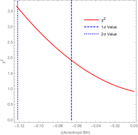
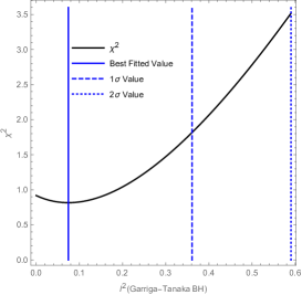
Figure 1: The left is $\chi^{2}$ for the parameter $\epsilon$ in the anisotropic black hole. The right is $\chi^{2}$ for the parameter $l^{2}$ in the Garriga-Tanaka black hole. The dashed lines denotes the $2\sigma$ value. The dotted lines denotes the $2\sigma$ value. The solid line denote the best fitted value.

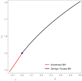
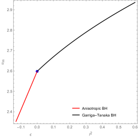
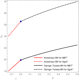
Figure 2: The strong deflection lensing coefficients $\bar{a}$, $\bar{b}$, and deflection angle $\alpha$ vs $\epsilon$ and $l^{2}$. The blue dot denotes the Schwarzchild  case. The $\epsilon$ parameter in the anisotropic black hole is in the constrained range $-0.12181<\epsilon<0$. The $l^{2}$ parameter in the Garriga-Tanaka black hole is $0<l^{2}<0.5901$.

Parameters	anisotropic BH			Schwarzschild BH	Garriga-Tanaka BH
	$\epsilon=-0.1218$	$\epsilon=-0.0655$	$\epsilon=-10^{-5}$		$l^{2}=0.0745$	$l^{2}=0.3609$	$l^{2}=0.5901$
$x_{m}$	$1.397$	$1.444$	$1.500$	$1.500$	$1.552$	$1.707$	$1.803$
$u_{m}(R_{s})$	$2.368$	$2.474$	$2.598$	$2.598$	$2.652$	$2.822$	$2.932$
$\bar{a}$	$1.039$	$1.020$	$1.000$	$1.000$	$0.9779$	$0.9285$	$0.9064$
$\bar{b}$	$-0.4319$	$-0.4160$	$-0.4004$	$-0.4002$	$-0.4112$	$-0.4567$	$-0.4870$
$\alpha$	$6.500$	$6.433$	$6.364$	$6.364$	$6.223$	$5.901$	$5.753$

Table 1: The values of parameters $x_{m}$, $u_{m}$, $\bar{a}$, $\bar{b}$ and $\alpha$ parameters. The $u_{m}$ is scaled by Schwarzschild radius $R_{s}=2GM_{\bullet}/c^{2}$.

Parameters	BH type	anisotropic BH			Schwarzschild BH	Garriga-Tanaka BH
		$\epsilon=-0.1218$	$\epsilon=-0.0655$	$\epsilon=-10^{-5}$		$l^{2}=0.0745$	$l^{2}=0.3609$	$l^{2}=0.5901$
$\theta_{\infty}~{}(\mu as)$	M87*	$18.15$	$18.96$	$19.91$	$19.91$	$20.33$	$21.63$	$22.47$
	Sgr $A^{*}$	$24.19$	$25.27$	$26.54$	$26.54$	$27.10$	$28.83$	$29.95$
$s~{}(nas)$	M87*	$28.34$	$26.64$	$24.91$	$24.92$	$21.63$	$15.23$	$12.82$
	Sgr $A^{*}$	$37.77$	$35.51$	$33.21$	$33.22$	$28.83$	$20.30$	$17.08$
$r~{}(mag)$	$-$	$6.565$	$6.688$	$6.822$	$6.822$	$6.976$	$7.347$	$7.526$
$\Omega_{m}$	$-$	$0.4223$	$0.4042$	$0.3849$	$0.3849$	$0.3770$	$0.3543$	$0.3411$
$\lambda$	$-$	$0.1265$	$0.1223$	$0.1176$	$0.1176$	$0.1166$	$0.1125$	$0.1096$
$\Delta T_{2,1}$	$-$	$15.14$	$15.80$	$16.57$	$16.57$	$16.90$	$17.92$	$18.59$
$\Delta T_{3,2}$	$-$	$14.89$	$15.56$	$16.33$	$16.33$	$16.67$	$17.74$	$18.43$
$\Delta T_{4,3}$	$-$	$14.88$	$15.54$	$16.32$	$16.32$	$16.67$	$17.73$	$18.42$
$\Delta T^{1}_{2,1}(10^{-3})$	$-$	$261.6$	$255.2$	$248.7$	$248.7$	$229.6$	$190.0$	$173.9$
$\Delta T^{1}_{3,2}(10^{-5})$	$-$	$1273$	$1173$	$1075$	$1075$	$924.3$	$644.8$	$543.3$
$\Delta T^{1}_{4,3}(10^{-7})$	$-$	$6191$	$5392$	$4644$	$4645$	$3720$	$2188$	$1697$

Table 2: The values of observables $\theta_{\infty}$, $s$, $r$, the QNM and the time delay parameters. The $\theta_{\infty}$ and $s$ are respectively in the units of micro-arcsecond ($\mu$as) and nano-arcsecond (nas). The time delay parameters $\Delta T_{n,m}$ and $\Delta T_{n,m}^{\ 1}$ are scaled by $2GM_{\bullet}/c^{3}\approx 42.45s$.

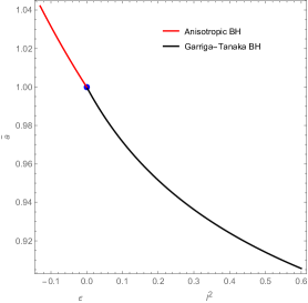
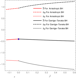
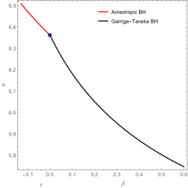
Figure 3: The strong deflection lensing coefficients $\bar{a}$, $\bar{b}$ (including $b_{R}$, $b_{0}$ as well) and deflection angle $\alpha$. The ranges of parameters are the same as FIG.2.

5.2 Discussions of the deflection angle in theory

Firstly, we list the deflection angle related parameter in TABLE 1. Then, we plot the shapes of the parameters $x_{m}$, $u_{m}$ and the observable $\theta_{\infty}$ in FIG.2 . The shapes of them are similar, all of them are increasing with respect to $\epsilon$ and $l^{2}$. In the case of Garriga-Tanaka black hole, the $x_{m}$, $u_{m}$ and $\theta_{\infty}$ parameters are always larger than the one of the Schwarzschild black hole with the same mass. While in the anisotropic black hole, $x_{m}$, $u_{m}$ and $\theta_{\infty}$ are smaller than the ones in Schwarzchild  black hole. The Schwarzchild  black hole connects the two braneworld black holes which denotes we could not distinguish the two braneworld black holes from the Schwarzchild  black hole. As $u_{m}$ is determined by the non-linear relation (Eq.(4.11)) with $x_{m}$, the slope of $u_{m}$ for the anisotropic black hole is smaller than that of Garriga-Tanaka black hole.

In Figure 3, the parameters $\bar{a}$ and $\bar{b}$ play a prominent role in measuring the angular difference from the outmost image and the adherent point related to the sequence of subsequent images. Roughly speaking, a bigger $u_{m}$ implies a smaller $\alpha$. Then the shape of $\bar{a}$ determines the shape of $\alpha$ which represents the divergence part. And the first term of $\alpha$ is more important than the other ones. Furthermore, corresponding to Eqs.(4.13) and (4.14), the divergent parts $\bar{a}$ and $b_{0}$ have a decreasing tendency, while the regular part $b_{R}$ contributes to the increasing tendency. The parameter $\bar{b}$, which presents the main part of the regular part, is one order lower than than $\alpha$, then its non-monotonic value does not affect $\alpha$. But, the shape of $\alpha$ parameter is not smooth as the $\bar{a}$.

5.3 The Observations

Besides $\theta_{\infty}$, there are other relations which could translate the $\bar{a}$ and $\bar{b}$ parameter to the observables, e.g. $s$, $r$, the time delays and the QNMs. We list all observables in TABLE 2 which shows the same tendencies.

5.3.1 The $s$ and $r$ parameter

The observable $s$ is the angular separation between the outermost image ($n=1$) and the packed others $n=2,3,....\infty$, and $r$ is the magnitude difference between the outermost image and the packed images,

$$s=\theta_{1}-\theta_{\infty}=\theta_{\infty}\exp{(\frac{\bar{b}}{\bar{a}}-\frac{2\pi}{\bar{a}})},$$ (5.3)

$$r=2.5\log_{10}(\frac{\mu_{1}}{\sum_{n=2}^{\infty}\mu_{n}})=2.5\log_{10}[\exp{(\frac{2\pi}{\bar{a}})}].$$ (5.4)

We plot the strong lensing coefficients and the value of the observables $s$, $r$ in FIG 4 as well. From FIG.4, the angular separation $s$ increases but angular position ($\theta_{\infty}$) and flux magnitude ($\mu$) decrease with respect to $\epsilon$ and $l^{2}$. The parameter $s$ is much smaller than $\theta_{\infty}$($1/1000$). As Eq.(5.3) shows, then $\theta_{1}$ are close to $\theta_{\infty}$. That means the $\theta_{\infty}$ parameter could present the main effect of angular separation. The parameter $s$ in anisotropic black hole is nearly linear, while in Garriga-Tanaka black hole is non-linear. The $s$ and $r$ are hard to observe because the magnitude ratio is proportional to the magnitude.

The $s$ is increasing with respect to $\epsilon$ and $l^{2}$, while the $r$ is decreasing. If we try to distinguish them via observation data, the accuracy of the measured separation between the first image and the surplus fringes needs to be less than $1\mu as$, and the photometric uncertainty has to better than $0.1$ mag.

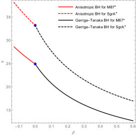
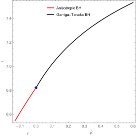
Figure 4: The estimated observables  $s$, $r$ as functions of $\epsilon$ (or $l^{2}$) for Anistropic Black hole (or Garriga-Tanaka Black Hole). The ranges of parameters are the same as FIG.2.

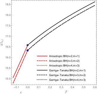
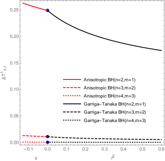
Figure 5: The estimated observables $\Delta T_{n,m}$ and $\Delta T_{n,m}^{\ 1}$ as functions of $\epsilon$ (or $l^{2}$) for Anistropic Black hole (or Garriga-Tanaka Black Hole). The ranges of obervables are the same as in FIG.2. $\Delta T_{n,m}$ and $\Delta T_{n,m}^{\ 1}$ are both represented in the unit of $2GM_{\bullet}/c^{3}\approx 42.45$ s.

5.3.2 The time delay

The time delays between relativistic images are observations as well. Bozza and Mancini obtain differential time delays among relativistic images due to gravitational lensing by a general static spherically symmetry spacetime [31]. The time delay is the result of the different paths followed by the photons while they cross around the black hole. Differences in the deflection angle are immediately displayed on the relativistic images[31]. If the mass and distance of the lens ( $D_{os}$) are known, then the any set of relativistic images could probe the type of black hole. $\Delta T_{n,m}$ is the total time delay between the $m$-loop image and the $n$-loop image

$$\Delta T_{n,m}=\Delta T^{0}_{n,m}+\Delta T^{1}_{n,m},$$ (5.5)

where leading term of time delay is

$$\Delta T^{0}_{n,m}=2\pi(n-m)u_{m},$$ (5.6)

while its much smaller correction is

$$\Delta T^{1}_{n,m}=2\sqrt{B_{m}/A_{m}}\sqrt{u_{m}/\hat{c}}\exp{(\bar{b}/(2\bar{a}))}[\exp{(-m\pi/\bar{a})}-\exp{(n\pi/\bar{a})}].$$ (5.7)

The unit of time delay is $2GM_{\bullet}/c^{3}\sim 42.45$ s. The dominant term in the time delay is not a new independent factor of the black hole. But the second term is. We consider three cases ( ($n=2,m=1$), ($n=3,m=2$), ($n=4,m=3$)) satisfying $n-m=1$ in which we consider two nearby loops and set same $T^{0}_{n,m}$. As shown in FIG. 5, the time delay in the two nearby loops is from $\Delta T^{1}_{n,m}$ which decreases to $0$ fast as $n$ increases. The same tendency occurs in the leading term $T_{n,m}$ when $n-m=1$, which is consistent with small $s$. The phenomenon shows there is no significant difference between the outmost image and the stacked images. Our present observational facilities do not reach the required resolution yet. For galactic black hole, the required resolution is of the order of $0.01$ micro-arcsecs. As the unit is $2GM_{\bullet}/c^{3}\sim 42.45$, the detection of $\Delta T_{2,1}$ needs to have an accuracy better than the level of $\sim 2\times 10^{-2}$ . After multiplying the units, it corresponds to the level of about $1s$ for Sgr A*.

5.3.3 The quasi normal modes (QNMs)

The strong lensing is useful to explain the characteristic modes of black hole as well. In Ref. [34, 35, 36], the quasi normal modes (QNMs) and the strong lensing are found to connect each other. The QNM describes the decay rates of perturbations around a black hole. It is expected to detect these perturbations in the further observations. At eikonal limit, the real and imaginary parts of the QNMs of any spherically symmetric, asymptotically flat spacetime are given by (multiples of) the frequency ($\Omega_{m}$) and instability timescale of the unstable circular null geodesics.

$$\omega_{QNM}=\Omega_{m}l-i(n+1/2)|\lambda|,$$ (5.8)

where $l$ and $n$ are constants and

$$\lambda=\frac{1}{u_{m}\bar{a}},$$ (5.9)

$$\Omega_{m}=1/u_{m}.$$ (5.10)

The real part of the complex QNM frequencies is determined by the angular velocity at the unstable null geodesic, the imaginary part the QNM is related to the instability timescale of the orbit which is called the Lyapunov exponent. The Lyapunov exponent is in turn reflected in the associated QNMs in the geometrical optical approximation. We list the values of QNMs in FIG.6. The tendencies of $\lambda$ and $\Omega_{m}$ are similar. For the Schwarzchild  model, it is the dot when $l^{2}=0$, while for the two branneworld black holes, it decreases with respect to $\epsilon$ and $l^{2}$. Our constrained Lyapunov exponents for M87* and SgrA* are positive. A positive Lyapunov exponent indicates a divergence between nearby trajectories, i.e., a high sensitivity to initial conditions.

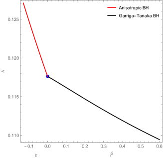
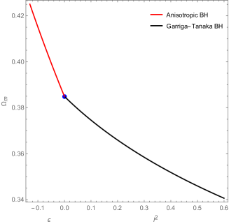
Figure 6: The estimated observables $\lambda$ and $\Omega_{m}$ as functions of $\epsilon$ (or $l^{2}$) for Anistropic Black hole (or Garriga-Tanaka Black Hole). The ranges of parameters are the same as in FIG.2.

5.4 A short summary

To derive the deflection angle, we need three parameter ($u_{m}$, $\bar{a}$ and $\bar{b}$). The observations $\theta_{\infty}$, $T_{n,m}$ and $\Omega_{m}$ are all related to $u_{m}$. The parameters $\lambda$ and $r$ are related to $\bar{a}$. The parameters $s$ and $\Delta T^{1}_{n,m}$ are related to $\bar{b}$. The Higher order effects, such as $s$, $r$, $\Delta T^{1}_{2,1}$ will distinguish the two black holes. We also show the total effect of $\alpha$. The non-linear relation between $u$ and $x_{m}$ make the non-smoothness between the the braneworld models.

6 Conclusion

In this work, based on the EHT data ($\theta_{\infty}$), we first use the $\chi^{2}$ test to estimate the range of parameters of braneworld black holes. Then, the $1\sigma$ and $2\sigma$ regimes of the model parameters are $\epsilon>-0.0655>-0.1218$ for the anisotropic black hole, and $l^{2}=0.0745^{+0.2864+0.5156}_{-0.0745-0.0745}$ for the Garriga-Tanaka black hole. The braneworld model are consistent with the observation which shows the braneworld black holes possess richer structure than ordinary black holes. And following the fitted data, we calculate the photon deflection angle, the angular separation, time delay values and QNM values between different relativistic images of the anisotropic black hole and the Garriga-Tanaka black hole. The anisotropic black hole and the Garriga-Tanaka black hole could not be distinguished by using observation data. And, this result is useful to probe extra dimension.

References

- [1] K . Akiyama et al. (Event Horizon Telescope), The Astrophysical Journal Letters, Volume 875: L1
- [2] K . Akiyama et al. (Event Horizon Telescope), The Astrophysical Journal Letters, Volume 875:L4
- [3] K . Akiyama et al. (Event Horizon Telescope), The Astrophysical Journal Letters, 930:L12
- [4] The Event Horizon Telescope Collaboration et al 2019 ApJL 875 L6
- [5] C. M. Will, Living Rev. Rel. 9 (2006), 3
- [6] S. Jordan, Astron. Nachr. 329 (2008), 875
- [7] S. G. Turyshev, et al., Int. J. Mod. Phys. D 16, 1879 (2008).
- [8] S. G. Turyshev, Ann. Rev. Nucl. Part. Sci. 58, 207 (2008).
- [9] L. Randall and R. Sundrum, Phys. Rev. Lett. 83 (1999), 4690-4693 doi:10.1103/PhysRevLett.83.4690 [arXiv:hep-th/9906064 [hep-th]].
- [10] A. Chamblin, S. W. Hawking and H. S. Reall, Phys. Rev. D 61 (2000), 065007 doi:10.1103/PhysRevD.61.065007 [arXiv:hep-th/9909205 [hep-th]].
- [11] T. Shiromizu, K. i. Maeda and M. Sasaki, Phys. Rev. D 62 (2000), 024012
- [12] R. Gregory, R. Whisker, K. Beckwith and C. Done, JCAP 10 (2004), 013 doi:10.1088/1475-7516/2004/10/013 [arXiv:hep-th/0406252 [hep-th]].
- [13] T. Tanaka, Prog. Theor. Phys. Suppl. 148 (2003), 307-316 doi:10.1143/PTPS.148.307 [arXiv:gr-qc/0203082 [gr-qc]].
- [14] S. Creek, R. Gregory, P. Kanti and B. Mistry, Class. Quant. Grav. 23 (2006), 6633-6658 doi:10.1088/0264-9381/23/23/004 [arXiv:hep-th/0606006 [hep-th]].
- [15] R. Maartens, Phys. Rev. D 62 (2000), 084023 doi:10.1103/PhysRevD.62.084023 [arXiv:hep-th/0004166 [hep-th]].
- [16] J. Garriga and T. Tanaka, Phys. Rev. Lett. 84 (2000), 2778-2781
- [17] S. B. Giddings, E. Katz and L. Randall, JHEP 03 (2000), 023 doi:10.1088/1126-6708/2000/03/023 [arXiv:hep-th/0002091 [hep-th]].
- [18] Dyson F W, EddinGarriga-Tanakaon A S and Davidson C 1920 Phil. Trans. Roy. Soc. Lond. A220 291
- [19] Zwicky F 1937 Phys. Rev. 51 290
- [20] A. Einstein, Science, 84, 506 (1936).
- [21] P. Schneider, J. Ehlers, and E. E. Falco, Gravitational Lenses (Springer-Verlag, Berlin, 1992).
- [22] A. O. Petters, H. Levine, and J. Wambsganss, Singularity Theory and Gravitational Lensing (Birkhauser, Boston, 2001).
- [23] V.Perlick,LivingRev.Relativity7,9(2004),http://relativity.livingreviews.org/Articles/lrr-2004-9.
- [24] P. Schneider, C. S. Kochanek, and J. Wambsganss, Gravitational Lensing: Strong, Weak and Micro, Lecture Notes of the 33rd Saas-Fee Advanced Course, edited by G. Meylan, P. Jetzer, and P. North (Springer-Verlag, Berlin, 2006).
- [25] C. Darwin, Proc. R. Soc. Lond. A 249 (1959); C. Darwin, Proc. R. Soc. Lond. A 263 (1961).
- [26] K. S. Virblack holeadra and G. F. R. Ellis, Phys. Rev. D 62 (2000), 084003
- [27] V. Bozza, S. Capozziello, G. Iovane and G. Scarpetta, Gen. Rel. Grav. 33 (2001), 1535-1548
- [28] V. Bozza, Phys. Rev. D 66 (2002), 103001 doi:10.1103/PhysRevD.66.103001 [arXiv:gr-qc/0208075 [gr-qc]].
- [29] V. Bozza, Gen. Rel. Grav. 42 (2010), 2269-2300
- [30] A. Chowdhuri, S. Ghosh and A. Bhattacharyya, Front. Phys. 11 (2023), 1113909 doi:10.3389/fphy.2023.1113909 [arXiv:2303.02069 [gr-qc]].
- [31] V. Bozza and L. Mancini, Gen. Rel. Grav. 36 (2004), 435-450
- [32] R. T. Cavalcanti, A. G. da Silva and R. da Rocha, Class. Quant. Grav. 33 (2016) no.21, 215007
- [33] S. G. Ghosh, R. Kumar and S. U. Islam, JCAP 03 (2021), 056
- [34] V. Cardoso, A. S. Miranda, E. Berti, H. Witek and V. T. Zanchin, Phys. Rev. D 79 (2009) no.6, 064016 doi:10.1103/PhysRevD.79.064016 [arXiv:0812.1806 [hep-th]].
- [35] S. R. Dolan and A. C. Ottewill, Class. Quant. Grav. 26 (2009), 225003 doi:10.1088/0264-9381/26/22/225003 [arXiv:0908.0329 [gr-qc]].
- [36] I. Z. Stefanov, S. S. Yazadjiev and G. G. Gyulchev, Phys. Rev. Lett. 104 (2010), 251103 doi:10.1103/PhysRevLett.104.251103 [arXiv:1003.1609 [gr-qc]].
- [37] X. J. Gao, J. M. Chen, H. Zhang, Y. Yin and Y. P. Hu, Phys. Lett. B 822 (2021), 136683 doi:10.1016/j.physletb.2021.136683 [arXiv:2108.09409 [gr-qc]].
- [38] Q. M. Fu and X. Zhang, Phys. Rev. D 105 (2022) no.6, 064020 doi:10.1103/PhysRevD.105.064020 Phys. Rev. D 106 (2022) no.6, 064010 doi:10.1103/PhysRevD.106.064010; X. J. Gao, X. k. Yan, Y. Yin and Y. P. Hu, Eur. Phys. J. C 83 (2023), 281 doi:10.1140/epjc/s10052-023-11414-0 [arXiv:2303.00190 [gr-qc]]; X. J. Gao, T. T. Sui, X. X. Zeng, Y. S. An and Y. P. Hu, Eur. Phys. J. C 83 (2023), 1052 doi:10.1140/epjc/s10052-023-12231-1 [arXiv:2311.11780 [gr-qc]].
- [39] N. Tsukamoto, Phys. Rev. D 95 (2017) no.6, 064035 doi:10.1103/PhysRevD.95.064035 [arXiv:1612.08251 [gr-qc]].
- [40] S. S. Zhao and Y. Xie, JCAP 07 (2016), 007
- [41] A. S. Majumdar and N. Mukherjee, Mod. Phys. Lett. A 20 (2005), 2487-2496
- [42] K. K. Nandi, Y. Z. Zhang and A. V. Zakharov, Phys. Rev. D 74 (2006), 024020
- [43] N. Tsukamoto, Phys. Rev. D 94 (2016) no.12, 124001 doi:10.1103/PhysRevD.94.124001 [arXiv:1607.07022 [gr-qc]].
- [44] G. O. de Xivry and P. Marshall, Mon. Not. Roy. Astron. Soc. 399 (2009), 2
- [45] S. E. Gralla, D. E. Holz and R. M. Wald, Phys. Rev. D 100 (2019) no.2, 024018
- [46] S. Ghosh and A. Bhattacharyya, JCAP 11 (2022), 006 doi:10.1088/1475-7516/2022/11/006 [arXiv:2206.09954 [gr-qc]].
- [47] M. Afrin and S. G. Ghosh, Astrophys. J. 932 (2022) no.1, 51 doi:10.3847/1538-4357/ac6dda [arXiv:2110.05258 [gr-qc]].
- [48] R. Kumar and S. G. Ghosh, Astrophys. J. 892 (2020), 78
- [49] R. C. Pantig and A. Övgün, [arXiv:2206.02161 [gr-qc]].
- [50] R. Whisker, Phys. Rev. D 71 (2005), 064004
- [51] C. R. Keeton and A. O. Petters, Phys. Rev. D 73 (2006), 104032 doi:10.1103/PhysRevD.73.104032 [arXiv:gr-qc/0603061 [gr-qc]].
- [52] A. Y. Bin-Nun, Phys. Rev. D 81 (2010), 123011
- [53] R. Whisker, [arXiv:0810.1534 [gr-qc]].
- [54] F. Dahia and A. de Albuquerque Silva, Eur. Phys. J. C 75 (2015) no.2, 87