Localized spatiotemporal dynamics in active fluids

Abstract

From cytoskeletal networks to tissues, many biological systems behave as active materials. Their composition and stress-generation is affected by chemical reaction networks. In such systems, the coupling between mechanics and chemistry enables self-organization, for example, into waves. Recently, contractile systems were shown to be able to spontaneously develop localized spatial patterns. Here, we show that these localized patterns can present intrinsic spatiotemporal dynamics, including oscillations and chaotic dynamics. We discuss their physical origin and bifurcation structure.

I Introduction

Self-organized oscillations are a common feature of living systems spanning a large range of scales, from genetic networks to animal populations [1]. In cells and tissues, such oscillations correlate with vital processes such as migration and cell division [2]. Although commonly analyzed in a pure chemical context, cellular oscillations often involve the mechanical units of the cytoskeleton [2, 3], a polymeric network consisting notably of actin filaments. From a physical point of view, the actin cytoskeleton is an active fluid, as various cortical processes driven by ATP hydrolysis can generate mechanical stress.

Many studies on mechanochemical oscillatory cellular dynamics and closely related waves focus on the actin cortex [4]. It is a thin layer of actin cytoskeleton beneath the plasma membrane of animal cells. Active cortical contractions coupled to actin-filament turnover can lead to sustained oscillations [5, 6, 7, 8, 9, 10, 11]. Furthermore, the cortex can exhibit spontaneous waves, in particular, in the context of cell migration [12, 13, 14, 15], but also during cell division [16].

Although cortical oscillations can be of purely mechanical origin [7, 17, 8, 18], the coupling of cytoskeletal dynamics to biochemical signaling networks is typically considered to be essential. Indeed, molecular networks establishing mutual feedback between the activity of signaling proteins and filament assembly as well as cytoskeletal contraction have been identified [16, 19, 20] and turn the actin cortex into an excitable medium [21, 22, 23].

Even in absence of active stress generation, the coupling between signaling modules and the cytoskeleton can lead to spontaneous (polymerization) waves [24, 25, 26, 27, 28]. Still, the fascinating dynamics of the actin cortex has led to the introduction and study of several theoretical descriptions combining the physics of active fluids and the dynamics of activity regulators [29, 30, 31, 32, 33, 34, 35, 36, 37].

In addition to cortical waves and oscillations that span the whole cell surface, experiments in adherent cells have identified oscillations that are localized in space [38, 19]. The mechanism underlying these dynamic states is currently unknown. We have recently shown that the coupling of active contractions and signaling reactions can lead to stationary localized states (LSs) [37]. Here, we extend our previous results and show that localized oscillatory states (LOSs) can spontaneously emerge on similar grounds.

II Mechanochemical theory of the cell cortex

To describe the dynamics of an active fluid coupled to a biochemical network, we combine active hydrodynamics with a reaction-diffusion system [36, 37]. The biochemical network is regulating assembly of the active material. In the case of the cortical actomyosin network in animal cells, this network would include small GTPases from the Ras and Rho families. These proteins exist in active and inactive states, where the former are typically attached to the cellular membrane and the latter are dissolved in the cytoplasm. In their active form, these small GTPases regulate factors promoting the nucleation and growth of actin filaments like formins or the Arp2/3 complex. In turn, the actomyosin network feeds back on the small GTPases’ activity.

Since here we are interested in studying generic properties of mechanochemical systems, we refrain from trying to give a comprehensive description of the biochemical regulatory network and their coupling to the cytoskeleton. Instead, we consider the active and inactive forms of some nucleation promoting factor – nucleator for short – and the active fluid. For the actin cortex it is appropriate to use an effective one-component description [39]. We thus introduce the corresponding densities $N_{a}$, $N_{i}$, and $C$. The time evolution of these densities is governed by mass-conservation laws. Explicitly, we use the equations introduced in Ref. [37],

$$\partial_{T}C+\nabla\cdot\bm{J}_{c} =AN_{a}-K_{d}C,$$ (1)

$$\partial_{T}N_{a}+\nabla\cdot\bm{J}_{a} =\Omega_{0}(1+\Omega N_{a}^{2})N_{i}-\Omega_{d}CN_{a},$$ (2)

$$\partial_{T}N_{i}+\nabla\cdot\bm{J}_{i} =-\Omega_{0}(1+\Omega N_{a}^{2})N_{i}+\Omega_{d}CN_{a},$$ (3)

where all quantities are dimensionless. As suggested by electron micrographs of the cortex [40], we consider the active fluid to be isotropic.

The current $\bm{J}_{c}=\bm{V}C-\mathscr{D}_{c}\nabla C$ for the active fluid consists of an advective and a diffusive term. Here, $\mathscr{D}_{c}$ is a diffusion constant, and $\bm{V}$ denotes the active fluid’s velocity field. The currents $\bm{J}_{a}$ and $\bm{J}_{i}$ for the active and inactive nucleators have the same form, but with different diffusion constants $\mathscr{D}_{a}$ and $\mathscr{D}_{i}$. Since active nucleators are bound to the membrane, whereas their inactive forms reside in the cytoplasm, we will consider $\mathscr{D}_{a}<\mathscr{D}_{i}$. In absence of advection, Eqs. (1)–(3) reduce to a reaction-diffusion system that has been used to describe actin polymerization waves [23].

The source and sink terms on the right hand sides account for transitions of nucleators between their active and inactive states as well as for the assembly and disassembly of the active fluid. The signs are chosen such that all corresponding parameters are positive. Specifically, $A$ is the rate of nucleation by active nucleators and $K_{d}$ the rate of spontaneous active fluid disassembly. The parameter $\Omega_{0}$ gives the rate of spontaneous nucleator activation. Experiments suggest that there is cooperative nucleator activation [41, 20] which we capture by the parameter $\Omega$. Furthermore, experiments show that there is negative feedback from the actomyosin on nucleator activity [41, 20]. We account for this effect through the parameter $\Omega_{d}$. Note that Eq. (2) and Eq. (3) conserve the total number of nucleators. Consequently, the average total nucleator density, $\bar{N}=(1/\mathcal{V})\int_{\mathcal{V}}(N_{a}+N_{i})d\mathcal{V}$, where $\mathcal{V}$ is the system volume, is constant. From now on, we consider the densities $C$, $N_{a}$, and $N_{i}$ to be scaled by $\bar{N}$, but keep the same notation as before. This rescaling implies that $\Omega_{d}\propto\bar{N}$ and $\Omega\propto\bar{N}^{2}$.

To close the dynamic equations, we use force balance, which captures momentum conservation in the case of low Reynolds number flows relevant for cortical actin dynamics. We choose [37]

$$\nabla\cdot\Sigma =\bm{V},$$ (4)

$$\Sigma =2\mathsf{V}+\left[\nabla\cdot\bm{V}+\Pi(C)\right]\mathds{1},$$ (5)

where $\Sigma$ is the stress tensor, $\mathsf{V}=(1/2)[\nabla\bm{V}+(\nabla\bm{V})^{T}-(\nabla\cdot\bm{V}/d)\mathds{1}]$ is the traceless strain rate tensor, $d$ the number of spatial dimensions and $\mathds{1}$ the identity. Finally, $\Pi(C)=\left(ZC^{2}-BC^{3}\right)\mathds{1}$ accounts for the non-viscous stress. If $Z,B>0$, then the first term can be interpreted as an active contractile stress, which dominates at low fluid densities, whereas hydrostatic contributions captured by the second term dominate at high densities [39]. Alternative forms of the non-viscous stress can be used [29]. Note that the scaling of the densities by $\bar{N}$ implies $Z\propto\bar{N}^{2}$ and $B\propto\bar{N}^{3}$.

Henceforth, we assume periodic boundary conditions. Our results are qualitatively similar if no-flux boundary conditions are assumed. Numerical solutions of Eqs. (1)–(5) are obtained using a custom code written in Julia [42], available online [43]. Unless specified otherwise, we use the parameter values: $\mathscr{D}_{c}=0.01$, $\mathscr{D}_{a}=0.1$, $\mathscr{D}_{i}=A=K_{d}=1$, $\Omega_{d}/\bar{N}=10$, $B/\bar{N}^{3}=Z/\bar{N}^{2},\bar{N}=1$. In Sect. III, we consider the dynamic Eqs. (1)–(5) in one spatial dimension. In Sect. IV, we treat the case of two spatial dimensions.

III Localized dynamic states in one dimension

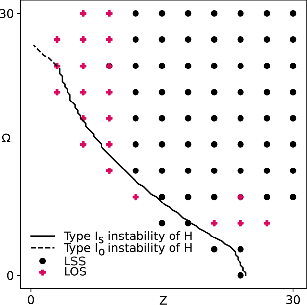
Figure 1: Phase diagram of localized states. Symbols indicate parameter values for which localized states (black circles: stationary, magenta crosses: oscillatory) are obtained through time evolution of a localized initial condition. Stationary and oscillatory localized states can coexist. Lines limit the region of linear stability of the homogenous stationary state (solid: Type $\mathrm{I_{s}}$ instability, dashed: Type $\mathrm{I_{o}}$ instability).

Consider a system of length $L=10\pi$. Eqs. (1)–(5) admit a unique homogenous state H with $C=AN_{a}/K_{d}$, $V=0$, $N_{i}=1-N_{a}$ and $N_{a}$ such that the right hand side of Eq. (2) vanishes [23]. A linear stability analysis shows that H becomes unstable if $Z$ and $\Omega$ exceed critical values, Fig. 1. The instability occurs at a finite wavelength, and can be either stationary or oscillatory, respectively, Type $\mathrm{I_{s}}$ and Type $\mathrm{I_{o}}$ in the language of Ref. [44].

The Type $\mathrm{I_{o}}$ instability is driven by the nonlinear chemical network and occurs in the range $0\leq Z\lesssim 3$. For $Z=0$ the system exhibits excitation waves [23]. For higher contractility, $Z\gtrsim 3$, H undergoes a Type $\mathrm{I_{s}}$ instability. Here, the instability is driven by the contractility and does not require a chemical network. In absence of a chemical network, local maxima in the fluid density emerge that fuse with time, such that eventually all the fluid is concentrated in a small region of space [29]. In the presence of both, contractility and a nonlinear chemical network, the critical values of the parameters decrease, and the instabilities are mechanochemical.

The traveling waves as well as the contracted states are spatially extended, in that they affect the fluid and nucleator densities throughout the whole system. In addition, there are localized states [37]. The existence of these states requires both, the contraction of the active fluid and the regulation of the fluid density through the chemical nucleator network.

Localized states can be stationary (localized stationary states, LSSs), as discussed in detail in Ref. [37], but also oscillatory (localized oscillatory states, LOSs). They exist in a large region of parameter space, Fig. 1. Furthermore, LSSs and LOSs can coexist. We find LOSs mostly for low contractility, in the proximity of the Type $\mathrm{I_{o}}$ instability of H. In the following, we discuss the emergence of LOSs in detail. We identify two distinct mechanism leading to LOSs. Either they emerge through a local instability of H or through a secondary instability of an LSS. The former dominates for low, whereas the latter dominates for high contractility. We discuss both instabilities in turn.

III.1 Low-contractility localized oscillations

In the vicinity of the critical parameter values for which the homogeneous state H loses linear stability, we also find an instability with respect to localized perturbations of finite amplitude. For low contractility, the states emerging from a localized perturbation are dominantly LOS. One example is illustrated in Fig. 2(a,b). For this state, a peak in the concentration of active nucleators emerges periodically in its center. It induces an increase in the density of the active fluid, then broadens, and splits. The two thus created peaks move at constant speed outward until they vanish at the state’s boundaries. For these internal “pulses”, a high nucleator concentration is present at the leading edge, followed by a region of high active fluid density, Fig. 2(b). This configuration is similar to that found in actin polymerization waves [23] and suggests a similar mechanism behind the motion of the peaks.

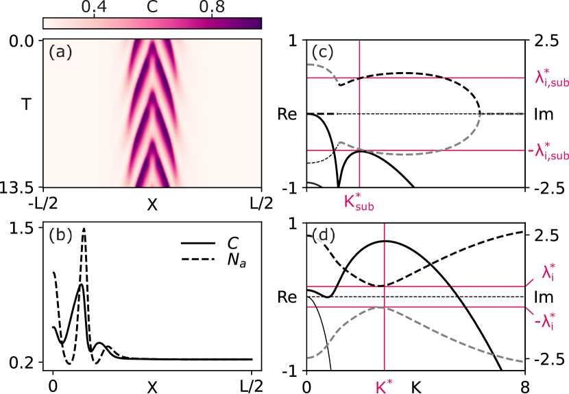
Figure 2: Localized oscillatory state at low contractility. (a) Kymograph of the active fluid denisty $C$. (b) Right half profile of the active fluid and active nucleator densities, at $T=0$ of panel (a). (c, d) Eigenvalues (full lines: real parts, dashed lines: imaginary parts) of Eqs. (1)–(5) linearized around H as a function of the non-dimensional wavenumber $K$. Parameters as in Sect. II, with $\Omega_{d}/\bar{N}=10$, $\Omega/\bar{N}^{2}=15$, $Z/\bar{N}^{2}=B/\bar{N}^{3}=6$, (a, b) $\bar{N}=1$ and (c) $\bar{N}=\bar{N}_{\mathrm{loc}}=1.38$.

For the parameter values chosen in Fig. 2, the state H is linearly stable, Fig. 2(c). When increasing the parameter $\Omega$ further, H undergoes a Type $\mathrm{I_{o}}$ instability. Yet, the origin of the LOSs can be traced back to the instability of a homogenous state. Indeed, the nondimensional parameters $\Omega$ and $Z$ varied in the stability diagram Fig. 1 depend both on the total average nucleator density $\bar{N}$ as $\Omega,Z\propto\bar{N}^{2}$. As a consequence, an instability can be induced by increasing the nucleator concentration. If localization of nucleators enhances the nucleator density sufficiently, one may expect the localized state to be patterned. This line of reasoning is similar to the one introduced in Refs. [45, 46], where patterns in a reaction-diffusion system subject to heterogeneous forcing were studied.

To explore this idea further, consider the region of high nucleator density, which in the example of Fig. 2 extends between the boundaries of the localized state $X_{l}=-5.09$ and $X_{r}=-X_{l}$. Concretely, the boundaries are defined as the points at which $N_{i}$ (the most diffusive, hence spread-out species) deviates more than $10\%$ from its value in the background, that is at $X=\pm L/2$. We can study the linear stability of the homogenous state that has a total density of nucleators equal to that within the localized state, $\bar{N}_{\mathrm{loc}}=\int_{X_{l}}^{X_{r}}(N_{a}+N_{i})dX/(X_{l}-X_{r})$. The corresponding growth exponents show that the homogenous state is linearly unstable and the eigenvalues with largest real part have a nonvanishing imaginary part, Fig. 2(d).

It is apparent from Fig. 2(d) that the system is well beyond the instability threshold. This is why one should not be surprised by the fact that the oscillation period deduced from the imaginary part of the fastest growing mode, $2\pi/\lambda_{i}^{*}=13.69$, does not capture well the period of the state in Fig. 2(a,b), which is $4.54$. Interestingly, a better estimate is obtained from the imaginary part of the same mode, but subthreshold, Fig. 2(c), where $2\pi/\lambda_{i,\mathrm{sub}}^{*}=5.25$.

III.2 High-contractility localized oscillations

At higher contractility, LOSs become less frequent, Fig. 1, and their profile changes. Two examples are illustrated in Fig. 3. Compared to their low-contractility counterparts, these LOSs are more confined in space. In terms of their time dependence, different states can be distinguished. The state in Fig. 3(a–c) exhibits weak oscillations composed of a single frequency and its harmonics. We refer to these as unimodal states. Conversely, the dependence on time of the state shown in Fig. 3(d–f) exhibits broader peaks as well as a band of modes with high frequency. This spectrum corresponds to intermittent bursts on top of regular oscillations. We refer to these as intermittent states.

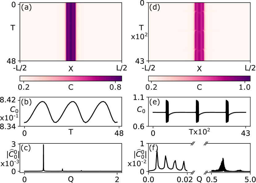
Figure 3: Localized oscillatory states at high contractility. (a, d) Kymographs of the active fluid denisty $C$. (b, e) Time series of the active fluid density $C_{0}=C(X=0,T)$. (d, f) Fourier spectrum $|\widehat{C_{0}^{0}}|$ of $C_{0}^{0}=C_{0}-\langle C_{0}\rangle_{T}$, where $\langle C_{0}\rangle_{T}$ is the temporal average of $C_{0}$. Q is the non-dimensional frequency. The horizontal axis of panel (f) is broken, and two different scales are used on the left and right sides. Parameters as in Sect. II, with $Z=15$, $\Omega=6.665$ (a) and $\Omega=6.666$ (b).

Differently from the low-contractility case, the LOSs in Fig. 3 are not the consequence of a local instability of H. Rather, they result from a secondary instability of an LSS. Some insight on this aspect can be gained from the bifurcation diagram in Fig. 4(a), which was obtained from numerical integration of the dynamic Eqs. (1)–(5). Branches were followed by taking the asymptotic solution for some parameter values as initial conditions for slightly different parameter values. Starting from an LSS solution and gradually increasing $\Omega$, a branch of unimodal LOSs emerges supercritically.

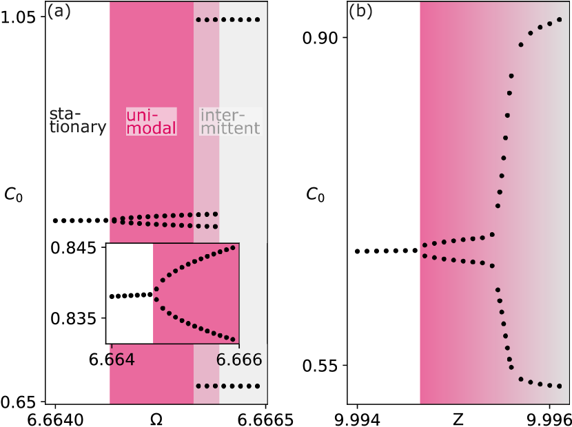
Figure 4: Bifurcation diagrams of oscillatory localized states. The two branches of oscillatory states represent, respectively, the maximum and minimum values attained by $C_{0}$, defined as in Fig. 3, during an oscillation. Parameters as in Sect. II, with $Z=15$ (a) and $\Omega=9$ (b).

When increasing $\Omega$ further, a branch of intermittent LOSs emerges subcritically. A similar sequence of states can be observed along different directions in parameter space, for instance using $Z$ as control parameter, Fig. 4(b). Although the qualitative behavior of the system is similar along the $\Omega$ and the $Z$ direction, the nature of the bifurcations can change. In particular, the transition from unimodal to intermittent LOSs can occur via a canard explosion [47], Fig. 4(b).

Further insight into the transition from LSS to LOS can be gained from a linear stability analysis of the LSS. We consider the fields

$$C =C^{0}(X)+\delta C(X,T),$$ (6)

$$N_{a} =N_{a}^{0}(X)+\delta N_{a}(X,T),$$ (7)

$$N_{i} =N_{i}^{0}(X)+\delta N_{i}(X,T),$$ (8)

$$V =V^{0}(X)+\delta V(X,T),$$ (9)

where the superscript $0$ denotes the LSS solution and the perturbative terms indicated by $\delta$ are assumed to be small compared to the LSS, but of the same order among each other.

For the numerical analysis of the LSS’s linear stability, we consider a discretized spatial grid $\bm{X}=(X_{1},X_{2},\dots X_{n})$, with spacing $\Delta X$ and $n=512$ sites. On this grid, spatial fields are represented as vectors with $n$ elements. We only retain terms linear in the perturbations. Note that we can then express $\delta\bm{V}$ in terms of $\delta\bm{C}$ by plugging Eqs. (6) and (9) into the force balance Eq. (4). Explicitly, we get

$$\delta\bm{V} =\mathds{S}\delta\bm{C},$$ (10)

$$\mathds{S} =\left(\mathds{1}-\mathds{D}_{2}\right)^{-1}\left[\mathrm{di}\left(\bm{\Pi}^{\prime}_{0}\right)\mathds{D}_{1}+\mathrm{di}\left(\bm{\Pi}^{\prime\prime}_{0}\right)\mathrm{di}\left(\mathds{D}_{1}\bm{C}_{0}\right)\right],$$ (11)

where $\mathds{D}_{n}$ is a finite difference operator that approximates an n-th spatial derivative in the discretized spatial grid. In particular, we use five-point stencil finite difference operators [48]. Furthermore, $\mathrm{di}(\bm{a})$ is an $n\times n$ matrix that is defined for a vector $\bm{a}$ as $\mathrm{di}(\bm{a})_{ij}=a_{i}$ if $i=j$ and $=0$ if $i\neq j$. Finally, $\bm{\Pi}^{\prime}_{0}$ and $\bm{\Pi}^{\prime\prime}_{0}$ are vectors corresponding to the discretized fields $\left(\partial\Pi/\partial C\right)\rvert_{C^{0}}$ and $\left(\partial^{2}\Pi/\partial C^{2}\right)\rvert_{C^{0}}$, respectively.

We use Eq. (10) to eliminate the velocity field from the linearized and discretized Eqs. 1–(3). This gives the following linear system:

$$\partial_{t}\begin{pmatrix}\delta\bm{C}\\ \delta\bm{N}_{a}\\ \delta\bm{N}_{i}\end{pmatrix}=\mathds{M}\begin{pmatrix}\delta\bm{C}\\ \delta\bm{N}_{a}\\ \delta\bm{N}_{i}\end{pmatrix}=\begin{pmatrix}\mathds{M}_{cc}&\mathds{M}_{ca}&\mathds{M}_{ci}\\ \mathds{M}_{ac}&\mathds{M}_{aa}&\mathds{M}_{ai}\\ \mathds{M}_{ic}&\mathds{M}_{ia}&\mathds{M}_{ii}\end{pmatrix}\begin{pmatrix}\delta\bm{C}\\ \delta\bm{N}_{a}\\ \delta\bm{N}_{i}\end{pmatrix}$$ (12)

where the vectors are defined as $(\delta C_{1},\cdots,\delta C_{N},\delta N_{a,1},\cdots\delta N_{a,N},\delta N_{i,1},\cdots\delta N_{i,N})$ and the $n\times n$ blocks $\mathds{M}_{ij}$, with $i,j\in\{c,a,i\}$, of the $3n\times 3n$ matrix $\mathds{M}$, can be found in Appendix A.

We compute the spectrum of $\mathds{M}$ for the LSS found for $Z=15$ and $\Omega=6.664$, the profile of which is given in Fig. 5(a). At $\Omega=6.67$, the LSS is linearly unstable. The instability is governed by a pair of complex-conjugate eigenvalues, $\lambda_{\pm}^{*}\equiv\lambda_{r}^{*}\pm i\lambda_{i}^{*}$, with $\lambda_{r}>0$, Fig. 5(b). Note that the eigenvalue $\lambda=0$ results from the conservation of nucleators.

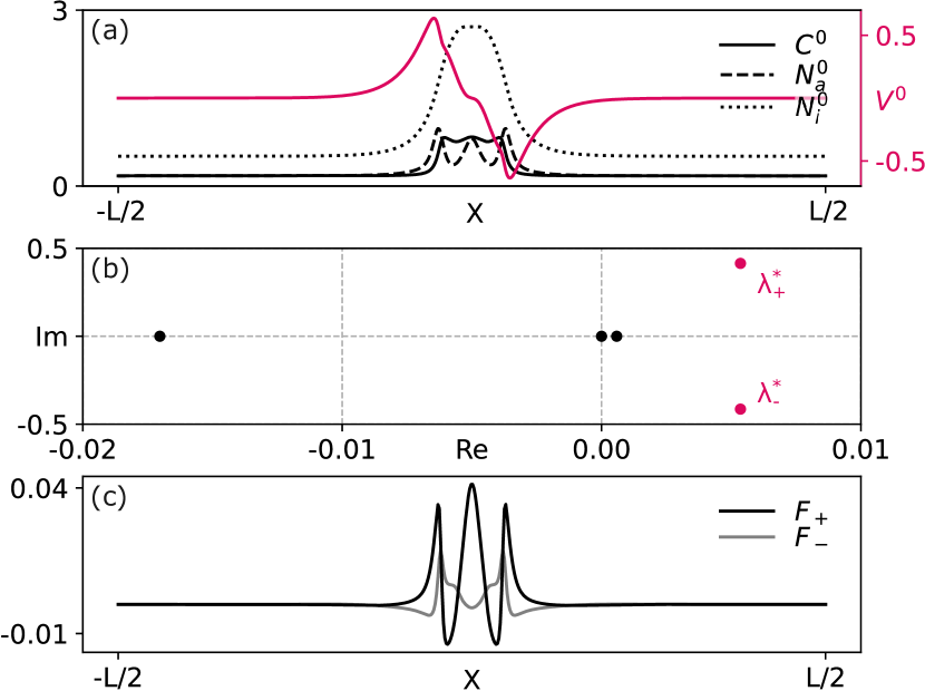
Figure 5: Linear oscillatory instability of a localized state. (a) Profile of the LSS for parameter values as in Fig. 4(a) and $\Omega=6.664$. (b) Leading eigenvalues of $\mathds{M}$, obtained by linearizing around the LSS in panel (a), for $\Omega=6.67$. (c) Real-valued $F_{+}=\left(f_{+}+f_{-}\right)/2$ and $F_{-}=\left(f_{+}-f_{-}\right)/2i$, where $f_{+}$ and $f_{-}$ are the eigenfunctions corresponding to $\lambda_{+}^{*}$ and $\lambda_{-}^{*}$ in panel (b), respectively. Only the components corresponding to $\delta\bm{C}$ are shown.

At $\Omega=6.67$, we estimate the oscillation period $\tau$ from the imaginary part of the eigenvalues, $\tau\approx 2\pi/\lambda^{*}_{\pm,i}=15.17$. This value is in very good agreement with the dominant mode of the LOS in Fig. 3(a–c), for which $\tau=15.34$. To further connect the LOS with the LSS, we consider the eigenfunctions $f_{+}$ and $f_{-}$ corresponding to $\lambda^{*}_{\pm}$. Through suitable linear combinations of $f_{+}$ and $f_{-}$, we obtain real-valued functions $F_{+}=\left(f_{+}+f_{-}\right)/2$ and $F_{-}=\left(f_{+}-f_{-}\right)/2i$. Their components corresponding to the density perturbation $\delta\bm{C}$ are given in Fig. 5(c). These functions are spatially localized within a region of width comparable to that of the LSS in Fig. 5(a). The oscillatory state is approximately given by the LSS plus $const.\times\left[\cos\left(2\pi T/\tau\right)F_{+}+\sin\left(2\pi T/\tau\right)F_{-}\right]$. This confirms that the LOS in Fig. 3(a–c) emerges from an instability of the LSS.

III.3 Chaotic localized states

In addition to the periodic LOSs discussed thus far, the dynamic Eqs. (1)–(3) also have more complicated localized solutions, Fig. 6(a). The width of the state shown is similar to that of LSS or LOS for similar values of $Z$. However, the concentration profile of the active fluid is irregular. The time-dependence of the active-fluid density $C_{0}=C(X=0,T)$ does not exhibit an easily recognizable pattern, Fig. 6(b), which is also expressed by its broad Fourier spectrum, Fig. 6(c).

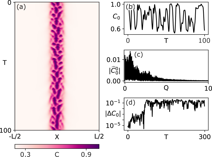
Figure 6: Chaotic localized state. (a) Kymograph of the active fluid density $C$. (b) Time series of the active density $C_{0}$, defined as in Fig. 3. (c) Fourier spectrum as defined in Fig. 3. (d) Absolute value of the difference between two time series $C_{0}$ with similar initial conditions. Vertical axis is in log scale. Parameters as in Sect. II, with $Z=9.3$ and $\Omega=12$.

This irregular localized state is likely chaotic. Indeed, for the corresponding parameter values, the absolute difference between $C_{0}$ for two slightly different initial conditions initially grows exponentially, Fig. 6(d). Specifically, we took the initial condition of the state shown in Fig. 6(a) and added two different weak white noise perturbations to it. Eventually, this difference saturates, which is an effect of the finite size of the attractor [49].

An in-depth characterization of this state as well as an exploration of the route to chaos is left for further studies.

IV Localized dynamic states in two dimensions

Similar to LSSs, LOSs persist in two spatial dimensions (2D). Much of the discussion of LOSs in 1D readily extends to the 2D case. Consider a square domain, $(X,Y)\in[-L/2,L/2]\times[-L/2,L/2]$, with periodic boundaries and $L=10\pi$. For low contractility, LOSs can take the form of target waves, Fig. 7(a). Note the similarity between the kymograph in Fig. 7(a) and that in Fig. 2(a). In the 2D case, however, at each instance in time, we observe typically more maxima in active fluid density as compared to the 1D case. Similarly to the 1D case, these maxima move outwards at constant velocity. The oscillation frequency is similar in 1D and 2D, whereas the spatial extension of the 2D state shown in Fig. 7(a) is larger than for the 1D state of Fig. 2 in spite of a larger contractility, $Z=9$ in 2D vs $Z=6$ in 1D.

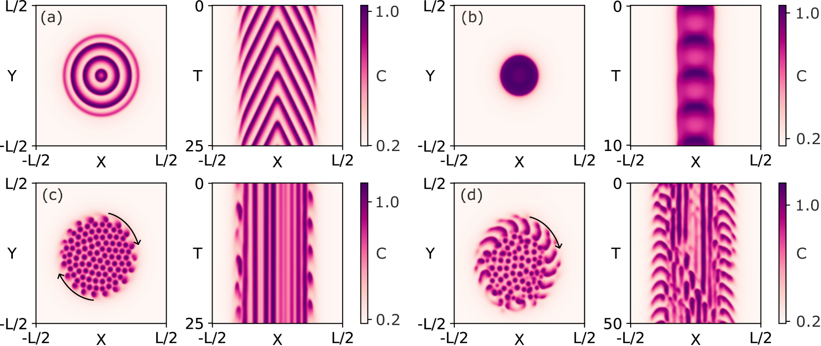
Figure 7: Localized oscillatory states in two dimensions. (a) Localized target wave. (b) Pulsating spot. (c) Closely packed spots, surrounded by a crown of sparser spots rotating clockwise (see arrows). (d) Dynamic multi-spot core surrounded by waves. The arrow indicates the direction of some wavefronts. (a–d) The kymographs on the left represent a cut of the 2D dynamics at $Y=0$. Parameters as in Sect. II, with $Z=9$, $\Omega=15$ (a), $Z=24$, $\Omega=3$ (b), $Z=12$, $\Omega=15$ (c), $Z=9$, $\Omega=18$ (d).

For higher contractility, LOSs can take the form of pulsating spots, Fig. 7(b). Similarly to the 1D case, these feature a stronger confinement as compared to their low-contractility counterparts.

There are also LOSs in 2D that do not have a 1D equivalent. In particular, localized states in 2D can spontaneously break chiral symmetry. In Fig. 7(c), a core of closely packed almost stationary spots is surrounded by a crown of spots traveling clockwise, around the central cluster. These traveling spots are less dense than the spots in the cluster, and feature a higher active fluid density towards their direction of motion.

Finally, 2D LOSs with an inner chaotic dynamics are also possible, Fig. 7(d).

V Conclusions

In this work, we have reported LOSs in a mechanochemical system, where active nucleators promote the assembly of an active fluid. Nucleators are advected by fluxes induced by active stress and are inactivated by the active fluid. We identified two possible origins of LOSs, namely, a local instability of the homogenous steady state and a secondary instability of LSSs.

LOSs similar to the ones discussed above were reported in a broad range of dissipative systems. For instance, in vertically vibrated granular layers [50], where they were termed ‘oscillons’. LSS-to-LOS instabilities and localized chaos were also reported in optical cavities [51, 52]. Localized spatiotemporal chaos was also realized in liquid crystals [53], where the resulting state was termed ‘chaoticon’.

Our choice of dynamic equations for the mechanochemical system is not unique [29, 31, 32, 33, 35, 36], and it will be interesting to investigate, which of the phenomena we report depend on details of the coupling between biochemistry and active mechanics. Even though these phenomena essentially rely on this coupling, it still seems reasonable to link at least the low contractility oscillations to an oscillatory chemical instability of the homogenous stationary state. Furthermore, in the parameter regions we investigated localization depends crucially on (active) contractility. We expect that a system exhibiting these two features – chemically induced oscillations and contractility – will generically have LOSs as solutions. Still, the explicit form of the kinetic rates and of the stress might affect these states.

Our theory is inspired by the actin cortex of animal cells. Following the remarks in the previous paragraph, localized oscillations could be a common feature of cortical actin. Indeed, LOSs we found could correspond to cortical structures reported in adhering cells [19, 38]. Our study thus suggests a strong link between these LOSs and spontaneous actin waves. By carefully tuning cortical contractility, cells might transition between these two classes of states. More experiments are needed to explore this connection further.

Appendix A Entries of $\mathds{M}$

In this appendix, we give the entries of the dynamic matrix $\mathds{M}$ appearing in Eq. (12).

$$\mathds{M}_{cc}= -\mathrm{di}\left(\mathds{D}_{1}\bm{C}^{0}\right)\mathds{S}-\mathrm{di}\left(\bm{C}^{0}\right)\mathds{D}_{1}\mathds{S}-\mathrm{di}\left(\mathds{D}_{1}\bm{V}^{0}\right)$$

$$-\mathrm{di}\left(\bm{V}^{0}\right)\mathds{D}_{1}+\mathscr{D}_{c}\mathds{D}_{2}+\mathrm{di}\left(\frac{\partial R_{c}}{\partial C}\Bigg{|}_{0}\right)$$ (13)

$$\mathds{M}_{ca}= \leavevmode\nobreak\ \mathrm{di}\left(\frac{\partial R_{c}}{\partial N_{a}}\Bigg{|}_{0}\right)$$ (14)

$$\mathds{M}_{ci}= \leavevmode\nobreak\ 0$$ (15)

$$\mathds{M}_{ac}= -\mathrm{di}\left(\mathds{D}_{1}\bm{N}^{0}_{a}\right)\mathds{S}-\mathrm{di}\left(\bm{N}_{a}^{0}\right)\mathds{D}_{1}\mathds{S}+\mathrm{di}\left(\frac{\partial R_{a}}{\partial C}\Bigg{|}_{0}\right)$$ (16)

$$\mathds{M}_{aa}= -\mathrm{di}\left(\mathds{D}_{1}\bm{V}^{0}\right)-\mathrm{di}\left(\bm{V}^{0}\right)\mathds{D}_{1}+\mathscr{D}_{a}\mathds{D}_{2}$$

$$+\mathrm{di}\left(\frac{\partial R_{a}}{\partial N_{a}}\Bigg{|}_{0}\right)$$ (17)

$$\mathds{M}_{ai}= \leavevmode\nobreak\ \mathrm{di}\left(\frac{\partial R_{a}}{\partial N_{i}}\Bigg{|}_{0}\right)$$ (18)

$$\mathds{M}_{ic}= -\mathrm{di}\left(\mathds{D}_{1}\bm{N}^{0}_{i}\right)\mathds{S}-\mathrm{di}\left(\bm{N}_{i}^{0}\right)\mathds{D}_{1}\mathds{S}+\mathrm{di}\left(\frac{\partial R_{i}}{\partial C}\Bigg{|}_{0}\right)$$ (19)

$$\mathds{M}_{ia}= \leavevmode\nobreak\ \mathrm{di}\left(\frac{\partial R_{i}}{\partial N_{a}}\Bigg{|}_{0}\right)$$ (20)

$$\mathds{M}_{ii}= -\mathrm{di}\left(\mathds{D}_{1}\bm{V}^{0}\right)-\mathrm{di}\left(\bm{V}^{0}\right)\mathds{D}_{1}+\mathds{D}_{2}+\mathrm{di}\left(\frac{\partial R_{i}}{\partial N_{i}}\Bigg{|}_{0}\right)$$ (21)

Here, $R_{c}=-K_{d}C+AN_{a}$, $R_{a}=-R_{i}=-\Omega_{d}CN_{a}+\Omega_{0}\left(1+\Omega N_{a}^{2}\right)N_{i}$, and $\lvert_{0}$ denotes derivatives evaluated at the LSS in Fig. 5(a). When the operator $\mathrm{di}\left(\cdot\right)$ is applied to a function of $X$, we implicitly assume a discretization of that function on the grid $\bm{X}$.

References

- Murray [1993] J. D. Murray, Mathematical Biology (Springer, Berlin, Heidelberg, 1993).
- Beta and Kruse [2017] C. Beta and K. Kruse, Intracellular Oscillations and Waves, Annual Review of Condensed Matter Physics 8, 239 (2017).
- Wu and Liu [2021] M. Wu and J. Liu, Mechanobiology in cortical waves and oscillations, Current Opinion in Cell Biology Cell Architecture, 68, 45 (2021).
- Yang and Wu [2018] Y. Yang and M. Wu, Rhythmicity and waves in the cortex of single cells, Philosophical Transactions of the Royal Society B: Biological Sciences 373, 20170116 (2018).
- Bornens et al. [1989] M. Bornens, M. Paintrand, and C. Celati, The cortical microfilament system of lymphoblasts displays a periodic oscillatory activity in the absence of microtubules: Implications for cell polarity., Journal of Cell Biology 109, 1071 (1989).
- Pletjushkina et al. [2001] O. J. Pletjushkina, Z. Rajfur, P. Pomorski, T. N. Oliver, J. M. Vasiliev, and K. A. Jacobson, Induction of cortical oscillations in spreading cells by depolymerization of microtubules, Cell Motility 48, 235 (2001).
- Paluch et al. [2005] E. Paluch, M. Piel, J. Prost, M. Bornens, and C. Sykes, Cortical Actomyosin Breakage Triggers Shape Oscillations in Cells and Cell Fragments, Biophysical Journal 89, 724 (2005).
- Sedzinski et al. [2011] J. Sedzinski, M. Biro, A. Oswald, J.-Y. Tinevez, G. Salbreux, and E. Paluch, Polar actomyosin contractility destabilizes the position of the cytokinetic furrow, Nature 476, 462 (2011).
- Solon et al. [2009] J. Solon, A. Kaya-Çopur, J. Colombelli, and D. Brunner, Pulsed Forces Timed by a Ratchet-like Mechanism Drive Directed Tissue Movement during Dorsal Closure, Cell 137, 1331 (2009).
- Martin et al. [2009] A. C. Martin, M. Kaschube, and E. F. Wieschaus, Pulsed contractions of an actin–myosin network drive apical constriction, Nature 457, 495 (2009).
- Westendorf et al. [2013] C. Westendorf, J. Negrete, A. J. Bae, R. Sandmann, E. Bodenschatz, and C. Beta, Actin cytoskeleton of chemotactic amoebae operates close to the onset of oscillations, Proceedings of the National Academy of Sciences 110, 3853 (2013).
- Vicker [2000] M. G. Vicker, Reaction–diffusion waves of actin filament polymerization/depolymerization in Dictyostelium pseudopodium extension and cell locomotion, Biophysical Chemistry 84, 87 (2000).
- Gerisch et al. [2004] G. Gerisch, T. Bretschneider, A. Müller-Taubenberger, E. Simmeth, M. Ecke, S. Diez, and K. Anderson, Mobile Actin Clusters and Traveling Waves in Cells Recovering from Actin Depolymerization, Biophysical Journal 87, 3493 (2004).
- Weiner et al. [2007] O. D. Weiner, W. A. Marganski, L. F. Wu, S. J. Altschuler, and M. W. Kirschner, An actin-based wave generator organizes cell motility, PLoS Biology 5, 2053 (2007).
- Stankevicins et al. [2020] L. Stankevicins, N. Ecker, E. Terriac, P. Maiuri, R. Schoppmeyer, P. Vargas, A.-M. Lennon-Duménil, M. Piel, B. Qu, M. Hoth, K. Kruse, and F. Lautenschläger, Deterministic actin waves as generators of cell polarization cues, Proceedings of the National Academy of Sciences 117, 826 (2020).
- Bement et al. [2015] W. M. Bement, M. Leda, A. M. Moe, A. M. Kita, M. E. Larson, A. E. Golding, C. Pfeuti, K.-C. Su, A. L. Miller, A. B. Goryachev, and G. von Dassow, Activator–inhibitor coupling between Rho signalling and actin assembly makes the cell cortex an excitable medium, Nature Cell Biology 17, 1471 (2015).
- Zumdieck et al. [2005] A. Zumdieck, M. C. Lagomarsino, C. Tanase, K. Kruse, B. Mulder, M. Dogterom, and F. Jülicher, Continuum Description of the Cytoskeleton: Ring Formation in the Cell Cortex, Physical Review Letters 95, 258103 (2005).
- Dierkes et al. [2014] K. Dierkes, A. Sumi, J. Solon, and G. Salbreux, Spontaneous Oscillations of Elastic Contractile Materials with Turnover, Physical Review Letters 113, 148102 (2014).
- Graessl et al. [2017] M. Graessl, J. Koch, A. Calderon, D. Kamps, S. Banerjee, T. Mazel, N. Schulze, J. K. Jungkurth, R. Patwardhan, D. Solouk, N. Hampe, B. Hoffmann, L. Dehmelt, and P. Nalbant, An excitable Rho GTPase signaling network generates dynamic subcellular contraction patterns, Journal of Cell Biology 216, 4271 (2017).
- Michaud et al. [2022] A. Michaud, M. Leda, Z. T. Swider, S. Kim, J. He, J. Landino, J. R. Valley, J. Huisken, A. B. Goryachev, G. von Dassow, and W. M. Bement, A versatile cortical pattern-forming circuit based on Rho, F-actin, Ect2, and RGA-3/4, Journal of Cell Biology 221, e202203017 (2022).
- Michaux et al. [2018] J. B. Michaux, F. B. Robin, W. M. McFadden, and E. M. Munro, Excitable RhoA dynamics drive pulsed contractions in the early C. elegans embryo, Journal of Cell Biology 217, 4230 (2018).
- Iglesias and Devreotes [2012] P. A. Iglesias and P. N. Devreotes, Biased excitable networks: How cells direct motion in response to gradients, Current Opinion in Cell Biology Cell Regulation, 24, 245 (2012).
- Ecker and Kruse [2021] N. Ecker and K. Kruse, Excitable actin dynamics and amoeboid cell migration, PLOS ONE 16, e0246311 (2021).
- Doubrovinski and Kruse [2008] K. Doubrovinski and K. Kruse, Cytoskeletal waves in the absence of molecular motors, EPL (Europhysics Letters) 83, 18003 (2008).
- Whitelam et al. [2009] S. Whitelam, T. Bretschneider, and N. J. Burroughs, Transformation from Spots to Waves in a Model of Actin Pattern Formation, Physical Review Letters 102, 198103 (2009).
- Carlsson [2010] A. E. Carlsson, Dendritic Actin Filament Nucleation Causes Traveling Waves and Patches, Physical Review Letters 104, 228102 (2010).
- Bernitt et al. [2017] E. Bernitt, H.-G. Döbereiner, N. S. Gov, and A. Yochelis, Fronts and waves of actin polymerization in a bistability-based mechanism of circular dorsal ruffles, Nature Communications 8, 15863 (2017).
- Yochelis et al. [2022] A. Yochelis, S. Flemming, and C. Beta, Versatile Patterns in the Actin Cortex of Motile Cells: Self-Organized Pulses Can Coexist with Macropinocytic Ring-Shaped Waves, Physical Review Letters 129, 088101 (2022).
- Bois et al. [2011] J. S. Bois, F. Jülicher, and S. W. Grill, Pattern Formation in Active Fluids, Physical Review Letters 106, 028103 (2011).
- Radszuweit et al. [2013] M. Radszuweit, S. Alonso, H. Engel, and M. Bär, Intracellular Mechanochemical Waves in an Active Poroelastic Model, Physical Review Letters 110, 138102 (2013).
- Kumar et al. [2014] K. V. Kumar, J. S. Bois, F. Jülicher, and S. W. Grill, Pulsatory Patterns in Active Fluids, Physical Review Letters 112, 208101 (2014).
- Banerjee et al. [2017] D. S. Banerjee, A. Munjal, T. Lecuit, and M. Rao, Actomyosin pulsation and flows in an active elastomer with turnover and network remodeling, Nature Communications 8, 1121 (2017).
- Nishikawa et al. [2017] M. Nishikawa, S. R. Naganathan, F. Jülicher, and S. W. Grill, Controlling contractile instabilities in the actomyosin cortex, eLife 6, e19595 (2017).
- Bhattacharyya and Yeomans [2021] S. Bhattacharyya and J. M. Yeomans, Coupling Turing stripes to active flows, Soft Matter 10.1039/D1SM01218E (2021).
- Staddon et al. [2022] M. F. Staddon, E. M. Munro, and S. Banerjee, Pulsatile contractions and pattern formation in excitable actomyosin cortex, PLOS Computational Biology 18, e1009981 (2022).
- del Junco et al. [2022] C. del Junco, A. Estevez-Torres, and A. Maitra, Front speed and pattern selection of a propagating chemical front in an active fluid, Physical Review E 105, 014602 (2022).
- Barberi and Kruse [2023a] L. Barberi and K. Kruse, Localized States in Active Fluids, Physical Review Letters 131, 238401 (2023a).
- Baird et al. [2017] M. A. Baird, N. Billington, A. Wang, R. S. Adelstein, J. R. Sellers, R. S. Fischer, and C. M. Waterman, Local pulsatile contractions are an intrinsic property of the myosin 2A motor in the cortical cytoskeleton of adherent cells, Molecular Biology of the Cell 28, 240 (2017).
- Joanny et al. [2013] J. F. Joanny, K. Kruse, J. Prost, and S. Ramaswamy, The actin cortex as an active wetting layer, The European Physical Journal E 36, 52 (2013).
- Fritzsche et al. [2016] M. Fritzsche, C. Erlenkämper, E. Moeendarbary, G. Charras, and K. Kruse, Actin kinetics shapes cortical network structure and mechanics, Science Advances 2, e1501337 (2016).
- Kamps et al. [2020] D. Kamps, J. Koch, V. O. Juma, E. Campillo-Funollet, M. Graessl, S. Banerjee, T. Mazel, X. Chen, Y.-W. Wu, S. Portet, A. Madzvamuse, P. Nalbant, and L. Dehmelt, Optogenetic Tuning Reveals Rho Amplification-Dependent Dynamics of a Cell Contraction Signal Network, Cell Reports 33, 108467 (2020).
- Bezanson et al. [2017] J. Bezanson, A. Edelman, S. Karpinski, and V. B. Shah, Julia: A Fresh Approach to Numerical Computing, SIAM Review 59, 65 (2017).
- Barberi and Kruse [2023b] L. Barberi and K. Kruse, Barberi-Kruse-PRL-2023, Zenodo (2023b).
- Cross and Hohenberg [1993] M. C. Cross and P. C. Hohenberg, Pattern formation outside of equilibrium, Reviews of Modern Physics 65, 851 (1993).
- Herschkowitz-Kaufman and Nicolis [1972] M. Herschkowitz-Kaufman and G. Nicolis, Localized Spatial Structures and Nonlinear Chemical Waves in Dissipative Systems, The Journal of Chemical Physics 56, 1890 (1972).
- Herschkowitz-Kaufman [1975] M. Herschkowitz-Kaufman, Bifurcation analysis of nonlinear reaction-diffusion equations—II. Steady state solutions and comparison with numerical simulations, Bulletin of Mathematical Biology 37, 589 (1975).
- Benoit et al. [1981] E. Benoit, J. L. Callot, F. Diener, and M. M. Diener, Chasse au canard, Collectanea Mathematica 32, 37 (1981).
- LeVeque [2007] R. J. LeVeque, Finite Difference Methods for Ordinary and Partial Differential Equations, Other Titles in Applied Mathematics (Society for Industrial and Applied Mathematics, 2007).
- Strogatz [2019] S. H. Strogatz, Nonlinear Dynamics and Chaos: With Applications to Physics, Biology, Chemistry, and Engineering, 2nd ed. (CRC Press, Boca Raton, 2019).
- Umbanhowar et al. [1996] P. B. Umbanhowar, F. Melo, and H. L. Swinney, Localized excitations in a vertically vibrated granular layer, Nature 382, 793 (1996).
- Leo et al. [2013] F. Leo, L. Gelens, P. Emplit, M. Haelterman, and S. Coen, Dynamics of one-dimensional Kerr cavity solitons, Optics Express 21, 9180 (2013).
- Parra-Rivas et al. [2021] P. Parra-Rivas, E. Knobloch, L. Gelens, and D. Gomila, Origin, bifurcation structure and stability of localized states in Kerr dispersive optical cavities, IMA Journal of Applied Mathematics 86, 856 (2021).
- Verschueren et al. [2013] N. Verschueren, U. Bortolozzo, M. G. Clerc, and S. Residori, Spatiotemporal Chaotic Localized State in Liquid Crystal Light Valve Experiments with Optical Feedback, Physical Review Letters 110, 104101 (2013).