Partial Fine-Tuning: A Successor to Full Fine-Tuning for Vision Transformers

Peng Ye¹^†, Yongqi Huang¹^†, Chongjun Tu¹,
Minglei Li¹, Tao Chen¹, Tong He², Wanli Ouyang²
¹Fudan University, ²Shanghai AI Laboratory Corresponding author. ^†Equal Contribution

Abstract

Fine-tuning pre-trained foundation models has gained significant popularity in various research fields. Existing methods for fine-tuning can be roughly divided into two categories, namely Parameter-Efficient Fine-Tuning and High-Performance Fine-Tuning. The former aims at improving efficiency, while the latter focuses on enhancing performance. Beyond these methods, we demonstrate that Partial Fine-Tuning can be an innovative and promising direction capable of concurrently enhancing both efficiency and accuracy. We first validate eight manually-defined partial fine-tuning strategies across kinds of datasets and vision transformer architectures, and find that some partial fine-tuning strategies (e.g., ffn only or attention only) can achieve better performance with fewer tuned parameters than full fine-tuning, and selecting appropriate layers is critical to partial fine-tuning. Thus, we propose a novel fine-tuned angle metric to guide the selection of appropriate layers for partial fine-tuning, making it flexible to be adapted to various scenarios for more practicable partial fine-tuning. Additionally, we show that partial fine-tuning can serve as a new dimension for Model Soups, improving both the model performance and generalization with fewer tuned parameters. Comprehensive experiments on a wide range of datasets and models validate the great potential of partial fine-tuning.

1 Introduction

Refer to caption — Figure 1: Performance comparisons of different kinds of fine-tuning methods, with a ViT-B/16 model pre-trained on ImageNet-21K and fine-tuned on ImageNet-1K. Our new perspective of partial fine-tuning (FAPFT, ATTN-only, and FFN-only) can improve both the performance and parameter efficiency of full fine-tuning, and be seamlessly combined with Model Soups (Soup-FAPFT). More similar comparisons are shown in the Appendix.

The integration of pre-training and fine-tuning has proven to be a successful approach in deep learning, facilitating the practical application of neural networks to a wide range of real-world problems. It has become a standard procedure in many domains and played a crucial role in advancing the state-of-the-art in various tasks [4, 8, 29, 22, 36, 37]. As the number of proposed pre-trained models continues to grow, how to effectively and efficiently adapt them to specific target tasks is attracting the increasing attention of researchers.

Existing fine-tuning methods can be roughly divided into two categories: Parameter-Efficient Fine-Tuning (PEFT) and High-Performance Fine-Tuning (HPFT). The former aims to improve the fine-tuning efficiency by freezing the pre-trained weights and fine-tuning only a few additional parameters [9, 15, 10]. The latter focuses on improving the model performance and generalization ability by combining model weights of multiple different fine-tuning [33, 26, 27]. Beyond these methods, a few recent works attempt to process partial parameters of the deep model. [28] transfers partial knowledge of the pre-trained CNN model for better few-shot learning. [30] finds that fine-tuning only the attention layers can adapt vision transformers. However, both methods focus on either specific tasks and networks or specific partial fine-tuning of specific architectures. As a result, there remains a need for more comprehensive research and development of general methods on partial fine-tuning.

To comprehensively understand the role of partial fine-tuning, we first manually define eight different partial fine-tuning strategies, and validate their effectiveness across kinds of datasets and vision transformer architectures. The experimental results show that: 1) The performance of different partial fine-tuning strategies is affected by both the architectures and the datasets. 2) Partial fine-tuning of specific functional layers (e.g., ffn or attention) of vision transformers produces comparable or even better results than full fine-tuning. 3) The position of partially fine-tuned layers of vision transformers has a significant impact on the performance. For more details, please refer to Sec. 3.1. These experiments and observations demonstrate the great potential of partial fine-tuning for achieving both high performance and parameter efficiency, while indicating that selecting appropriate layers is critical to improving the effectiveness and extending the utility of partial fine-tuning.

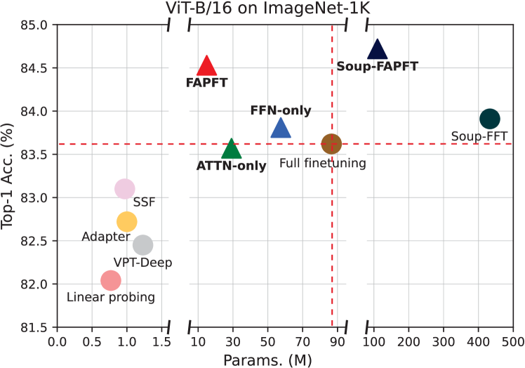
To this end, we develop a general and practicable partial fine-tining method based on a novel fine-tuned angle metric. Firstly, we define the fine-tuned angle metric as the angle between pre-trained and fine-tuned weights of a specific layer since it can measure the training behavior during fine-tuning. Then, we compute and rank the fine-tuned angles of all layers under different kinds of fine-tuning configures (i.e., various hyper-parameters, epochs, and datasets), and find that different layers in the model may have different but constant effects when fine-tuning on a specific dataset. Further, we treat the layer with a large fine-tuned angle as the influential one and the layer with a small fine-tuned angle as the redundant one, and propose to fine-tune only the influential parts for challenging tasks to adapt most effectively, and fine-tune only the redundant parts for easy tasks to maintain the pre-trained knowledge maximally. As shown in Fig. 1, although some manually-selected partial fine-tuning may already perform better than full fine-tuning, fine-tuned angle guided partial fine-tuning can surpass them on both the performance and parameter efficiency.

We conduct comprehensive experiments on kinds of datasets and models to validate the superiority of the proposed method. The results show that the proposed method can not only reduce the parameter number but also improve the performance. Our novelties can be summarized as: 1) We in-depth investigate the role of partial fine-tuning for different vision transformers and datasets for the first time, and demonstrate its great potential for high-performance parameter-efficient fine-tuning. 2) We propose a novel fine-tuned angle guided partial fine-tuning approach, which is more effective and practicable by automatically selecting appropriate layers for fine-tuning in various scenarios. 3) We show that partial fine-tuning can serve as a new dimension for Model Soups, and is complementary to the common practice of using different training configures.

2 Related Work

2.1 Fine-tuning Methods

The current research on model fine-tuning methods can be broadly divided into two main streams: Parameter-Efficient Fine-Tuning (PEFT) and High-Performance Fine-Tuning (HPFT). Beyond these two directions, we show that Partial Fine-Tuning can be a novel and promising direction.

Parameter-Efficient Fine-Tuning (PEFT) is a recent technique that aims to adapt pre-trained models to new tasks while fine-tuning only a few additional parameters. In early attempts, a low-rank FFN module called Adapter is introduced by [9] and inserted between transformer layers, greatly improving the parameter efficiency of fine-tuning. In parallel, Prefix-tuning [18] and VPT [15] splice special prefix tokens into the input and only update the embedding of these unique prefix tokens when fine-tuning. Besides, LoRA [10] injects the rank-decomposition matrix into Transformer blocks as bypass modules and only finetunes these modules. Afterward, countless variations via these methods are proposed and applied to various tasks [21, 12, 13].

High-Performance Fine-Tuning (HPFT) focuses on maximizing performance by utilizing model weights of multiple fine-tuning. Model Soups [33] averages weights obtained by fine-tuning the same pre-trained model with different configures, improving performance without additional inference costs. DiWA [26] employs diverse weight averaging for better generalization, especially for out-of-distribution (OOD) data. Model Ratatouille [27] reuses the weights obtained by first fine-tuning on multiple auxiliary tasks and then fine-tuning on the target task, further enhancing the OOD generalization ability.

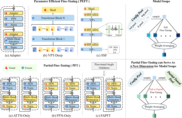
Besides, recent studies processing partial parameters of deep models have brought new insights into fine-tuning. For better few-shot learning, [28] transfers partial knowledge from the base set to the novel set by setting different learning rates for different layers of the pre-trained CNN model. [30] indicates that merely fine-tuning the weights of attention layers can already adapt ViTs to different resolutions and classification tasks. However, the former places its emphasis on the few-shot task and CNN model, and the latter focuses on the specific partial fine-tuning of ViTs. Differently, we present the first comprehensive study of partial fine-tuning, validating the effectiveness of various partial fine-tuning on a range of datasets and models. We also introduce a novel fine-tuned angle guided partial fine-tuning strategy and find that partial fine-tuning can serve as a new dimension for Model Soups. We show the details in Fig. 2.

2.2 Angle Metric and Its Applications

Recently, the deep learning community has recognized the significance of angle metric in evaluating the training behavior of neural networks. Several studies [1, 19] have theoretically demonstrated that the angle of model weights provides an accurate measure of weight updates. In [2], the angle metric is proposed, which is defined as the angle between the initialized weights and that of a well-trained network and is used to assess the network’s generalization capability. Further, ABS [11] introduces the angle metric to represent the whole model performance and utilizes it to shrink the search space of Neural Architecture Search (NAS), RLNAS [38] employs such angle metric to search for the optimal architecture, and AngleLoss [35] discusses the impact on NAS when applying the angle metric to the feature extraction and prediction layers respectively. Unlike the above methods that use the angle metric to indicate the performance or generalization of different architectures or operators, we explore how to leverage it to guide partial fine-tuning. Besides, all the above methods measure the angle between the initialized and well-trained model weights, while we explore the angle of each layer between pre-trained and fine-tuned model weights. Since such a finetuned angle metric has not been studied before, we conduct some empirical studies and show some interesting findings.

3 Method

3.1 Partial Fine-Tuning Is All You Need

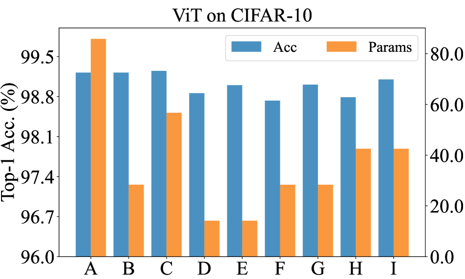
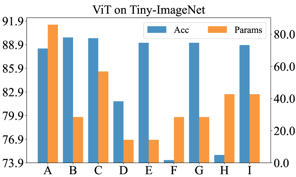
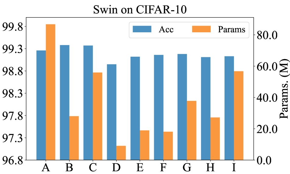
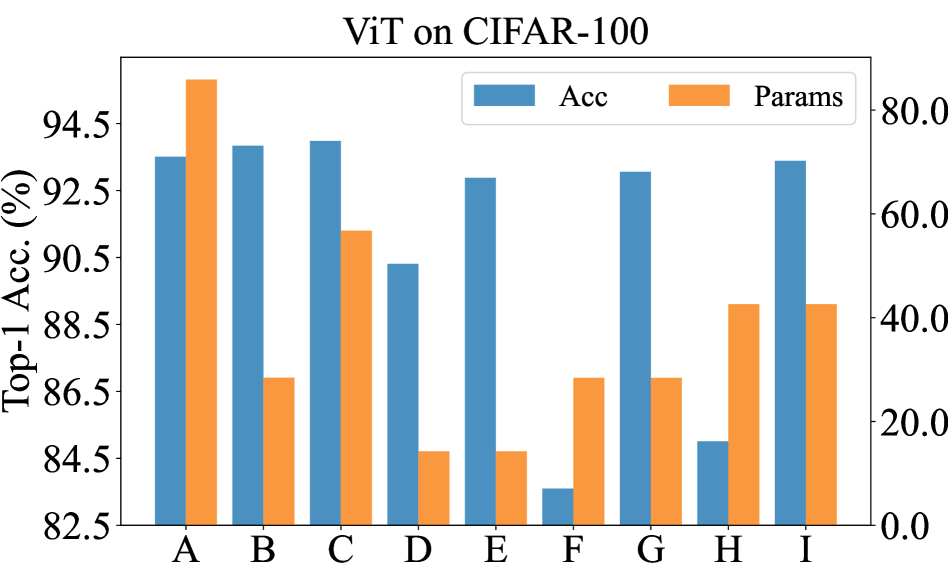
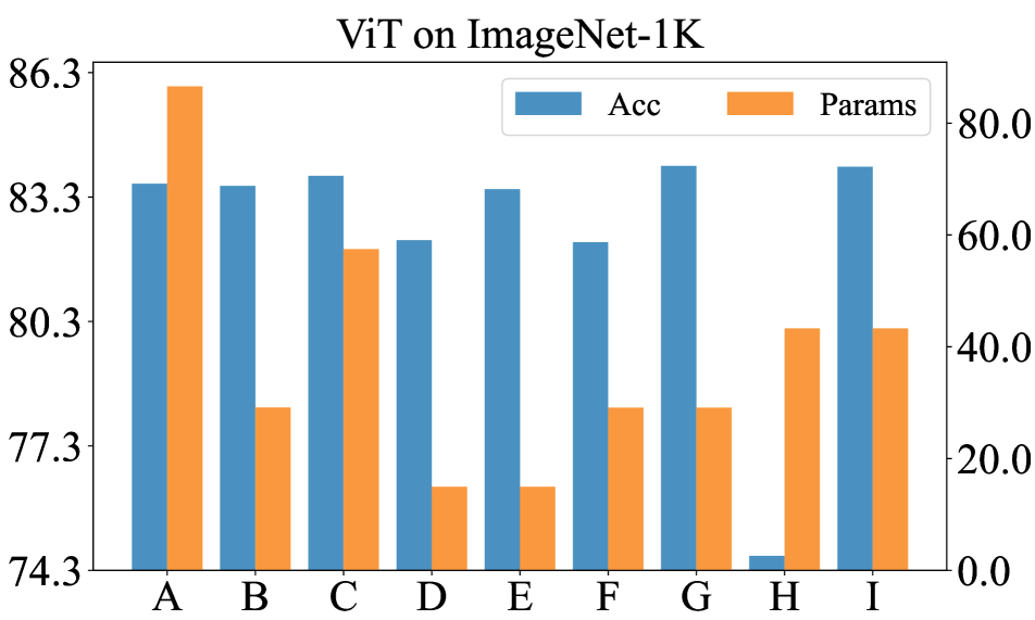
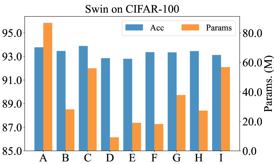
To gain a more comprehensive understanding of partial fine-tuning, we conduct several exploratory experiments across various datasets (CIFAR-10, CIFAR-100, Tiny-ImageNet, and ImageNet-1K) and vision transformer architectures (ViT, and Swin Transformer). In each task setting, we compare the performance and number of trainable parameters between full fine-tuning and eight different partial fine-tuning strategies. The results are shown in Fig. 3, from which we can conclude three insightful observations.

Insightful Observation 1: The performance of different partial fine-tuning strategies is influenced by both the architecture and dataset. First, the optimal partial fine-tuning strategy differs across different architectures and datasets. Second, different architectures and datasets have different sensitivities to partial fine-tuning. For example, the performance differences for all partial fine-tuning strategies are small for ViT on CIFAR-10, Swin on CIFAR-10, and Swin on CIFAR-100, while relatively large for other strategies.

Insightful Observation 2: Partial fine-tuning of specific functional layers of vision transformers yields comparable or even better results than full fine-tuning. This is particularly evident when examining the performance of fine-tuning only the attention layers or the ffn layers, which substantially reduce the trainable parameters while preserving satisfactory results. This phenomenon also validates the great potential of partial fine-tuning.

Insightful Observation 3: The position of the fine-tuned layers of various vision transformers plays a significant role in the performance of partial fine-tuning. For example, with the same trainable parameters, fine-tuning only the latter half of layers consistently performs better than fine-tuning only the first half of layers, which is especially apparent when considering the fine-tuned results of ViT on CIFAR-100, Tiny-ImageNet, and ImageNet-1K datasets.

In light of these observations, a strategy to select appropriate layers for fine-tuning in various scenarios becomes crucial to extending the utility of partial fine-tuning.

3.2 Fine-tuned Angle guided Partial Fine-Tuning

Based on the observations in Sec. 3.1, when proper parts are chosen for kinds of datasets and architectures, partial fine-tuning can achieve comparable performance with fewer parameters than full fine-tuning. Thus, we shift our attention to how to select proper parts for partial fine-tuning.

Since the angle metric is widely used for evaluating the training behavior of neural networks, we introduce it to measure the impact of various fine-tuning configures on different layers of the given model. Original angle metric, which is utilized for either indicating the generalization capacity of a model [1, 19] or ranking candidate architectures in NAS [11, 38, 35], converts the weights of a whole network into a one-dimensional vector, and computes the angle between the weight vectors before and after training. In detail, given a model $M$ , let $\boldsymbol{W}_{\mathbf{0}}$ and $\boldsymbol{W}_{\mathbf{t}}$ denotes its initialization weight vector and trained weight vector respectively, then the original angle metric can be computed as

\theta(\boldsymbol{M})=\arccos\left(\frac{\boldsymbol{W}_{\mathbf{0}}\cdot\boldsymbol{W}_{\boldsymbol{t}}}{\|\boldsymbol{W}_{\mathbf{0}}\|_{2}\|\boldsymbol{W}_{\boldsymbol{t}}\|_{2}}\right)

(1)

Fine-tuned Angle Metric. As we want to investigate the training behavior of each layer when fine-tuning the model, which has not been explored before, we first define a new fine-tuned angle metric. For a specific layer $L$ in the model, we convert its pre-trained weights and fine-tuned weights into a one-dimensional vector respectively, denoted as $\boldsymbol{W}_{\mathbf{p}}^{L}$ and $\boldsymbol{W}_{\mathbf{f}}^{L}$ , then the fine-tuned angle metric are calculated as

\theta(\boldsymbol{L})=\arccos\left(\frac{\boldsymbol{W}_{\mathbf{p}}^{L}\cdot\boldsymbol{W}_{\boldsymbol{f}}^{L}}{\|\boldsymbol{W}_{\mathbf{p}}^{L}\|_{2}\|\boldsymbol{W}_{\boldsymbol{f}}^{L}\|_{2}}\right)

(2)

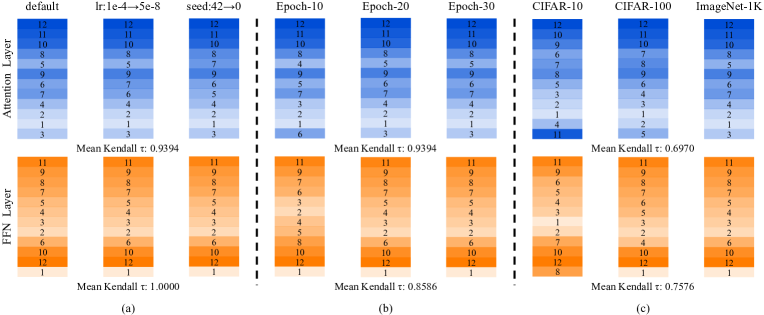
Fine-tuned Angle of Various Configures. We then compute the fine-tuned angles of different layers of the model under different fine-tuning configures. For a comprehensive study, we explore the effect of kinds of fine-tuning hyperparameters, iterations, and datasets. The results are shown in Fig. 4. As we can see, the ranking of the fine-tuning angles of all layers is surprisingly consistent under different fine-tuning hyperparameters and iterations (as shown in Fig. 4 (a) and (b)), while different fine-tuning datasets result in very different rankings of the fine-tuning angles of all layers (as shown in Fig. 4 (c)). Such results reveal that different layers in the model may have different but constant effects on the fine-tuning process for a specific dataset, which further inspires us to consider using such fine-tuned angle as a kind of guidance for partial fine-tuning.

Fine-tuned Angle guided Partial Fine-Tuning. Recent works have investigated the difference value between the pre-trained model weights and the fine-tuned one and further regarded the large difference value as the influential one and the small difference value as the redundant one [14, 34]. Inspired by this, we also treat the layer with a large fine-tuned angle as the influential layer and the layer with a small fine-tuned angle as the redundant layer. Further, for challenging tasks, we can fine-tune only the influential parts (layers with large fine-tuned angles) to adapt most effectively. For easy tasks, we can fine-tune only the redundant parts (layers with small fine-tuned angles) to maintain the pre-trained knowledge maximally. In the experiments section, we show the effectiveness of such a strategy, which performs much better than manually selected partial fine-tuning strategies on kinds of datasets and architectures.

Model	ViT-B/16 [6]				Swin-B [23]				ConvNeXt-B [24]				AS-MLP-B [20]
	CIFAR-100	Params. (M)	ImageNet-1K	Params. (M)	CIFAR-100	Params. (M)	ImageNet-1K	Params. (M)	CIFAR-100	Params. (M)	ImageNet-1K	Params. (M)	CIFAR-100	Params. (M)
Full fine-tuning	93.51	85.88	83.62	86.57	93.77	86.85	85.07	87.77	94.04	87.67	85.49	88.59	90.04	86.83
Linear probing	88.70	0.08	82.04	0.77	89.27	0.10	83.25	1.03	89.20	0.10	84.05	1.03	79.04	0.10
Adapter [9]	93.34	0.31	82.72	1.00	92.49	0.33	83.82	1.26	92.86	0.45	84.49	1.37	88.01	0.33
VPT-Deep [15]	93.17	0.54	82.45	1.23	92.62	0.70	83.44	1.63	-	-	-	-	-	-
SSF [21]	93.99	0.28	83.10	0.97	93.06	0.37	84.40	1.29	93.45	0.36	84.85	1.28	88.28	0.37
ATTN-Only	93.84	28.44	83.57	29.14	93.46	28.16	84.58	29.08	-	-	-	-	-	-
FFN-Only	93.98	56.76	83.81	57.46	93.88	56.02	84.88	56.95	-	-	-	-	-	-
FAPFT (ours)	94.30	49.69	84.53	14.95	94.07	33.61	85.17	42.01	94.05	45.19	85.38	39.76	90.74	46.21

Table 1: Performance comparisons of diverse fine-tuning approaches across different model architectures on CIFAR-100 and ImageNet-1K. Except for the AS-MLP-B model, which is pre-trained on ImageNet-1K, the other models, including ViT-B/16, Swin-B, and ConvNeXt-B, are pre-trained on ImageNet-21K. Each partial fine-tuning utilizes the same hyper-parameters as full fine-tuning, while others do not.

	CUB-200 -2011	NABirds	Oxford Flowers	Stanford Dogs	Stanford Cars	Mean	Params. (M)
Full fine-tuning	87.30	82.70	98.80	89.40	84.50	88.54	85.98
Linear probing	85.30	75.90	97.90	86.20	51.30	79.32	0.18
Adapter [9]	87.10	84.30	98.50	89.80	68.60	85.67	0.41
VPT-Deep [15]	88.50	84.20	99.00	90.20	83.60	89.11	0.85
SSF [21]	82.70	85.90	98.50	87.70	82.60	87.48	0.39
ATTN-Only	87.95	83.52	98.93	89.52	87.48	89.48	29.14
FFN-Only	86.23	83.24	98.81	90.14	83.75	88.43	57.46
FAPFT (ours)	88.68	83.79	99.04	91.20	88.15	90.17	30.69

Table 2: Performance comparisons of diverse fine-tuning strategies across five FGVC datasets, using ViT-B/16 model pre-trained on ImageNet-21K as the backbone. To guarantee a fair comparison, the results for the SSF method presented in the table are replicated from [5], which uses the same fundamental data augmentations as others. Note that PEFT methods (Adapter, VPT-Deep, and SSF) employ a grid search for each task to optimize hyper-parameters, while partial fine-tuning methods use identical hyper-parameters as full fine-tuning.

Method	FFT		FAPFT
Exp.	Acc.	Params.	Acc.	Params.
run1	83.61	86.57	84.25	7.86
run2	83.66	86.57	84.53	14.95
run3	83.62	86.57	84.42	22.03
run4	83.45	86.57	84.37	29.12
run5	83.86	86.57	84.20	36.21
Soup	83.91	432.9	84.72	110.2

(a)

Method	FFT		FAPFT
Exp.	Acc.	Params.	Acc.	Params.
run1	93.95	85.88	93.53	14.25
run2	93.45	85.88	93.69	21.34
run3	93.81	85.88	94.09	28.43
run4	93.51	85.88	94.15	35.52
run5	93.14	85.88	94.30	49.69
Soup	94.05	429.4	94.37	146.2

(b)

Method	FFT		FAPFT
Exp.	Acc.	Params.	Acc.	Params.
run1	84.98	87.77	85.04	29.39
run2	84.99	87.77	85.12	32.54
run3	84.93	87.77	85.17	42.01
run4	85.01	87.77	85.17	51.47
run5	85.07	87.77	85.11	57.78
Soup	85.18	438.9	85.25	213.2

(c)

Method	FFT		FAPFT
Exp.	Acc.	Params.	Acc.	Params.
run1	93.68	86.85	94.00	32.62
run2	93.57	86.85	94.07	33.61
run3	93.65	86.85	94.03	35.78
run4	93.77	86.85	94.02	36.77
run5	93.56	86.85	93.86	45.23
Soup	93.91	434.3	94.14	184.0

(d)

Table 3: Comparisons of full fine-tuning (FFT) based and FAPFT based Model Soups. We present the results of 5 individual runs for both methods, subsequently amalgamating them into Model Soups. The final row provides the final performance and the total parameters. Our FAPFT-based soup shows better performance and fewer parameters than FFT-based soup across various models and datasets.

	IN-1K ( $\uparrow$ )	IN-A ( $\uparrow$ )	IN-R ( $\uparrow$ )	IN-C ( $\downarrow$ )	Params.
Full fine-tuning	83.62	37.36	53.75	43.40	86.57
ATTN-Only	83.57	42.33	55.51	42.16	29.14
FFN-Only	83.81	40.35	54.47	42.77	56.76
FAPFT (ours)	84.53	45.00	55.04	41.38	14.95
Soup-FFT	83.91	41.40	55.39	41.84	432.9
Soup-FAPFT	84.72	46.67	56.23	40.08	110.2

(a)

	IN-1K ( $\uparrow$ )	IN-A ( $\uparrow$ )	IN-R ( $\uparrow$ )	IN-C ( $\downarrow$ )	Params.
Full fine-tuning	85.07	48.39	58.39	44.23	87.77
ATTN-Only	84.58	50.16	57.82	44.36	29.08
FFN-Only	84.88	49.81	58.63	43.93	56.95
FAPFT (ours)	85.17	50.17	57.20	43.91	42.01
Soup-FFT	85.18	50.99	58.98	43.06	438.9
Soup-FAPFT	85.25	51.71	58.22	42.80	213.2

(b)

Table 4: Comparisons of the robustness and generalization. ViT-B/16 and Swin-B models are pre-trained on ImageNet-21K. ’IN’ denotes ImageNet. Performance metrics include Top-1 accuracy (%) for IN-1K, IN-A, and IN-R datasets, with higher values (

\uparrow

) indicating better performance, and mean Corruption Error (mCE) for IN-C, with lower values (

\downarrow

) indicating better performance.

3.3 Partial Fine-Tuning can Serve As A New Dimension for Model Soups

Model Soups [33] improves the model performance and generalization ability by averaging weights fine-tuned with different configures. Its subsequent variations [26, 27] focus on designing different training configures to diversify the averaged weights for better results. Although the training configures may differ, all the weights used in these methods are fully fine-tuned. In this paper, we claim and show that partial fine-tuning can serve as a new dimension for Model Soups, which provides a fresh perspective for future research in this direction.

4 Experiments

4.1 Experimental Settings

Datasets. We evaluate our method on a variety of datasets, which can be categorized into: 1) General Classification Datasets. To assess the effectiveness of FAPFT, we conduct experiments on commonly used image classification datasets, namely CIFAR-100 [17] and ImageNet-1K [3]. 2) FGVC Datasets. We further extend our method to five Fine-Grained Visual Classification (FGVC) datasets to showcase its advantages, including NABirds [31], CUB-200-2011 [32], Oxford Flowers [25], Stanford Dogs [16], and Stanford Cars [7].

Models. To show the generalization ability of our method, we conduct experiments on four different backbones: plain transformer-based ViT/B-16 [6], hierarchical transformer-based Swin-B [23], CNN-structured ConvNeXt-B [24], and MLP-structured AS-MLP-B [20]. Note that AS-MLP-B is pre-trained on ImageNet-1K while the others are pre-trained on ImageNet-21K.

Baselines. In this study, we benchmark our approach with two basic fine-tuning methods as well as three parameter-efficient solutions: 1) Full fine-tuning, which updates all model parameters. 2) Linear probing, which only updates the classifier’s parameters. 3) Adapter [12], which only updates parameters in inserted low-rank FFN modules. 4) VPT [15], which only updates newly incorporated prompt tokens. 5) SSF [21], which only updates linear transformation parameters for modulating features.

Implementation Details. For general datasets, in line with SSF [21], we train for 100 epochs with a 10 epoch warm-up on CIFAR-100, 30 epochs with a 5 epoch warm-up on ImageNet-1K, and employ the same strong data augmentation strategy. For five FGVC datasets, following VPT [15], we train for 100 epochs with a 10 epoch warm up on each FGVC dataset and adopt the same standard augmentations. For all experiments, we utilize the AdamW optimizer and the cosine decay learning rate scheduler.

In our partial fine-tuning strategies, pre-trained weights are selectively frozen at the layer level, where a layer refers to an entire residual-connected unit. For instance, a ViT’s attention layer comprises a multi-head attention module and its preceding normalization layer, as depicted in Fig. 2. Further, we define layers with identical structures and parameter counts as the homogeneous group. For example, in the ViT model, all FFN layers form a single homogeneous group, while in the Swin model, homogeneous FFN layers are segregated by stage. More details can be found in the Appendix.

For FAPFT deployment, we start with a fully fine-tuned model tailored to the specific dataset and architecture. By comparing this model to its pre-trained counterpart, we compute fine-tuned angles and subsequently organize layers into their respective homogeneous groups. Within each group, we select the top k layers with the largest or smallest angles for targeted partial fine-tuning.

Notably, across all datasets and model architectures, each of our partial fine-tuning methods utilizes the same hyper-parameters as those applied in full fine-tuning and defaults to freezing non-residual modules.

4.2 Experiments on Image Classification

We conduct extensive experiments across a wide range of datasets, including CIFAR-100, ImageNet-1K, and various FGVC datasets, utilizing various architectures such as ViT, Swin, ConvNeXt, and AS-MLP. The results, detailed in Tab. 1 and Tab. 2, consistently verify that Fine-tuned Angle guided Partial Fine-Tuning (FAPFT) surpasses in achieving both high accuracy and improved parameter efficiency.

Tab. 1 shows the effectiveness of FAPFT on general datasets. As we can see, PEFT methods fall short of surpassing the baseline of full fine-tuning on the ImageNet-1K dataset. As a comparison, the hand-designed partial fine-tuning strategies of ATTN-Only and FFN-Only demonstrate comparable or even better performance with fewer parameters than full fine-tuning. Further, the proposed FAPFT approach achieves even better results, for the ViT model, even surpasses the baseline method by a significant margin. Moreover, FAPFT possesses greater universality and also works for other architectures like ConvNeXt-B and AS-MLP-B. Additionally, on the CIFAR-100 dataset, FAPFT also outperforms other approaches consistently, confirming its robustness with different datasets.

As Tab. 2 indicates, all three partial fine-tuning strategies (ATTN-Only, FFN-Only, and FAPFT) perform well on the five FGVC datasets, and averaged results highlight the benefits of partial fine-tuning than full fine-tuning. Although hand-designed ATTN-Only and FFN-Only methods can achieve good performance, the proposed FAPFT method stands out as the most effective, delivering a significant improvement of 90.17% compared to 88.64% with remarkably fewer parameters (30.69M VS 85.98M).

4.3 Experiments on Model Soups

In this section, we show how the proposed FAPFT approach can serve as a new dimension for Model Soups. We conduct experiments using ViT-B/16 and Swin-B models on ImageNet-1K and CIFAR-100 datasets to showcase the superiority of FAPFT over full fine-tuning (FFT) in the model soups context. Specifically, we conduct five runs for each method with distinct configures, concluding with an aggregated soup. FFT’s experiments vary in hyper-parameters, such as learning rate and seed. For FAPFT, we maintain consistent hyper-parameters across experiments, only altering the number of layers to be fine-tuned.

As shown in Tab. 3, individual runs highlight FAPFT’s consistent outperformance in both model accuracy and parameter efficiency, ultimately resulting in Soup-FAPFT surpassing Soup-FFT in both metrics. Notably, compared to Soup-FFT based on the ViT-B/16 model on ImageNet-1K and CIFAR-100 datasets, Soup-FAPFT achieves an accuracy gain of 0.81% and 0.32%, alongside a significant parameter reduction of 322.7 and 283.2 million, respectively. Further, Soup-FAPFT consistently outperforms Soup-FFT for the Swin-B model on different datasets while maintaining parameter efficiency. These results indicate the potential of FAPFT to not only strengthen individual fine-tuned models but also uplift the collective performance for the Model Soups framework in a parameter-efficient manner.

4.4 Experiments on Robustness and OOD Datasets

We further evaluate the robustness and Out-Of-Distribution (OOD) capabilities of the proposed FAPFT method on ImageNet-A, ImageNet-R, and ImageNet-C datasets. All models are fine-tuned on ImageNet-1K. Results are listed in Tab. 4. In most scenarios, partial fine-tuning methods (namely ATTN-Only, FFN-Only, and our FAPFT) always yield models with better robustness and OOD generalization compared to full fine-tuning. For example, ViT-B/16 finetuned via FAPFT shows a 0.91% increase in IID accuracy on ImageNet-1K as well as notable gains of 7.43%, 1.29%, and 1.99% on ImageNet-A/R/C respectively. These gains likely stem from FAPFT’s uniqueness in fine-tuning only the most influential layers, ensuring the most effective adaptation for challenging tasks. Furthermore, when combined with Model Soups, the resultant averaged model consistently outperforms its individual counterpart across all metrics. What’s more, the FAPFT-based soup achieves comprehensive improvements with reduced computation cost over the full fine-tuning (FFT) based soup, across various model architectures and datasets.

4.5 Ablation Studies

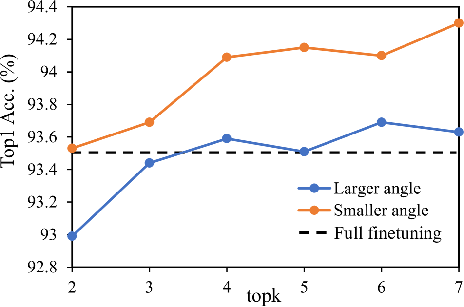
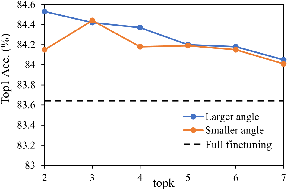
In this section, we explore two critical components in the proposed FAPFT strategy, e.g., the magnitude of the fine-tuned angle for layer selection (larger or smaller angle) and the number of layers to be fine-tuned (top-k). We conduct experiments using the ViT-B/16 model on CIFAR-100 and ImageNet-1K datasets to gain insights into their impact on performance. Results are presented in Fig. 10. For the easier dataset of CIFAR-100, fine-tuning layers with smaller fine-tuned angles consistently leads to significantly better performance than fine-tuning layers with larger fine-tuned angles. Conversely, on the more complex dataset of ImageNet-1K, fine-tuning layers with larger fine-tuned angles is more advantageous, which performs better across multiple top-k values and attains a notable peak performance of 84.53% in the setting of top2 larger angles. These observations further confirm the idea of our FAPFT method: partial finetuning based on smaller fine-tuned angles benefits the simpler datasets or tasks since it can maximally maintain the pre-trained knowledge, whereas partial finetuning based on larger angles benefits the more complex datasets or tasks since it can realize the most effective adaptation.

4.6 Computational cost

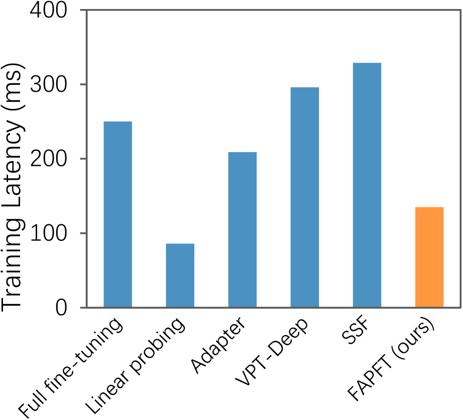
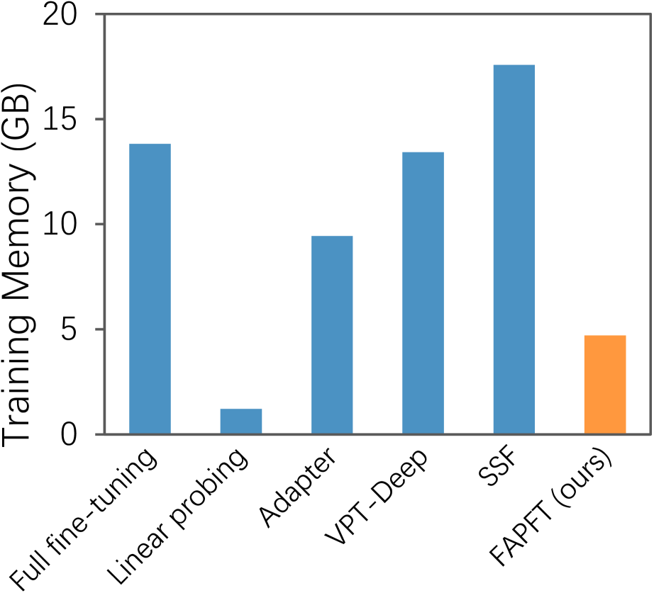
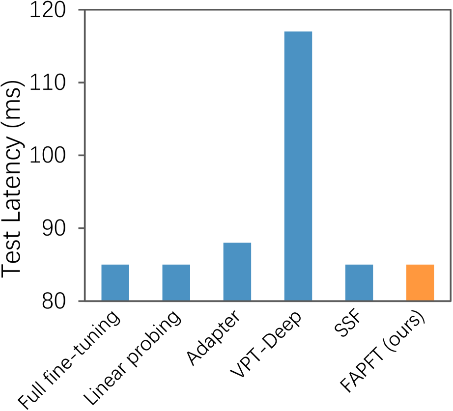
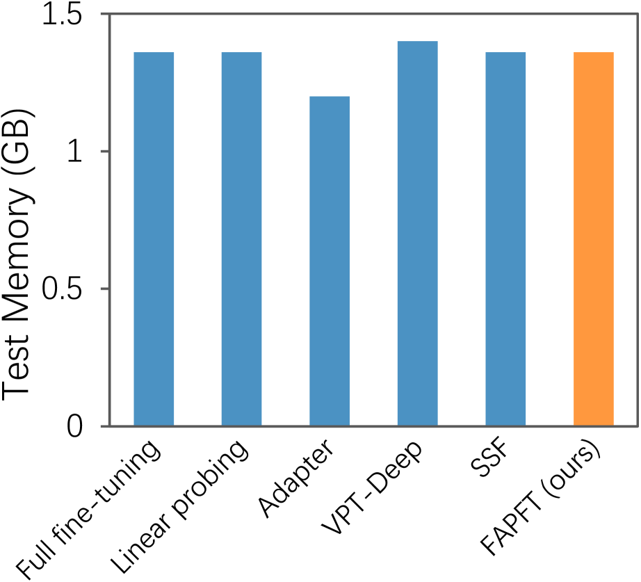
To evaluate the efficiency of the proposed FAPFT, we compare the computational cost of various fine-tuning methods in Fig. 8. We conduct the training and inference stages using a batch size of 128 and employ mixed precision training. All measurements are obtained using a single NVIDIA A100 GPU with 80GB of GPU memory. To ensure a fair comparison, we utilize identical settings to those used for ViT-B/16 on ImageNet-1K in Tab. 1. Specifically, we employ a reduction factor of 64 for the Adapter and 50 prompts for VPT-Deep. As we can see, most methods require additional cost. For example, Adapter increases the test latency, VPT-Deep increases the training latency, test latency, and test memory, while SSF increases the training latency and training memory. As a comparison, FAPFT exhibits much lower training latency and memory, and the same test latency and memory, demonstrating its great potential for future research and practical applications.

5 Conclusion

In this paper, we present partial fine-tuning as an innovative and promising approach capable of concurrently improving performance and parameter efficiency. We first find that partial fine-tuning of specific functional layers can achieve better performance with fewer tuned parameters than full fine-tuning, and selecting appropriate layers has a substantial impact on partial fine-tuning. Further, we propose a general partial fine-tuning method via a novel fine-tuned angle metric, adaptively selecting more appropriate layers in various scenarios. Extensive experiments across diverse datasets and architectures validate the substantial potential of partial fine-tuning.

References

Arora et al. [2018] Sanjeev Arora, Zhiyuan Li, and Kaifeng Lyu. Theoretical analysis of auto rate-tuning by batch normalization. arXiv preprint arXiv:1812.03981, 2018.
Carbonnelle and De Vleeschouwer [2019] Simon Carbonnelle and Christophe De Vleeschouwer. Layer rotation: a surprisingly simple indicator of generalization in deep networks? In ICML 2019 Workshop on Identifying and Understanding Deep Learning Phenomena, 2019.
Deng et al. [2009] Jia Deng, Wei Dong, Richard Socher, Li-Jia Li, Kai Li, and Li Fei-Fei. Imagenet: A large-scale hierarchical image database. In 2009 IEEE conference on computer vision and pattern recognition, pages 248–255. Ieee, 2009.
Devlin et al. [2018] Jacob Devlin, Ming-Wei Chang, Kenton Lee, and Kristina Toutanova. Bert: Pre-training of deep bidirectional transformers for language understanding. arXiv preprint arXiv:1810.04805, 2018.
Dong et al. [2023] Wei Dong, Dawei Yan, Zhijun Lin, and Peng Wang. Efficient adaptation of large vision transformer via adapter re-composing. arXiv preprint arXiv:2310.06234, 2023.
Dosovitskiy et al. [2020] Alexey Dosovitskiy, Lucas Beyer, Alexander Kolesnikov, Dirk Weissenborn, Xiaohua Zhai, Thomas Unterthiner, Mostafa Dehghani, Matthias Minderer, Georg Heigold, Sylvain Gelly, et al. An image is worth 16x16 words: Transformers for image recognition at scale. arXiv preprint arXiv:2010.11929, 2020.
Gebru et al. [2017] Timnit Gebru, Jonathan Krause, Yilun Wang, Duyun Chen, Jia Deng, and Li Fei-Fei. Fine-grained car detection for visual census estimation. In Proceedings of the AAAI Conference on Artificial Intelligence, 2017.
He et al. [2022] Kaiming He, Xinlei Chen, Saining Xie, Yanghao Li, Piotr Dollár, and Ross Girshick. Masked autoencoders are scalable vision learners. In Proceedings of the IEEE/CVF conference on computer vision and pattern recognition, pages 16000–16009, 2022.
Houlsby et al. [2019] Neil Houlsby, Andrei Giurgiu, Stanislaw Jastrzebski, Bruna Morrone, Quentin De Laroussilhe, Andrea Gesmundo, Mona Attariyan, and Sylvain Gelly. Parameter-efficient transfer learning for nlp. In International Conference on Machine Learning, pages 2790–2799. PMLR, 2019.
Hu et al. [2021] Edward J Hu, Yelong Shen, Phillip Wallis, Zeyuan Allen-Zhu, Yuanzhi Li, Shean Wang, Lu Wang, and Weizhu Chen. Lora: Low-rank adaptation of large language models. arXiv preprint arXiv:2106.09685, 2021.
Hu et al. [2020] Yiming Hu, Yuding Liang, Zichao Guo, Ruosi Wan, Xiangyu Zhang, Yichen Wei, Qingyi Gu, and Jian Sun. Angle-based search space shrinking for neural architecture search. In Computer Vision–ECCV 2020: 16th European Conference, Glasgow, UK, August 23–28, 2020, Proceedings, Part XIX 16, pages 119–134. Springer, 2020.
Hu et al. [2023] Zhiqiang Hu, Yihuai Lan, Lei Wang, Wanyu Xu, Ee-Peng Lim, Roy Ka-Wei Lee, Lidong Bing, and Soujanya Poria. Llm-adapters: An adapter family for parameter-efficient fine-tuning of large language models. arXiv preprint arXiv:2304.01933, 2023.
Huang et al. [2023] Chengsong Huang, Qian Liu, Bill Yuchen Lin, Tianyu Pang, Chao Du, and Min Lin. Lorahub: Efficient cross-task generalization via dynamic lora composition. arXiv preprint arXiv:2307.13269, 2023.
Ilharco et al. [2022] Gabriel Ilharco, Marco Tulio Ribeiro, Mitchell Wortsman, Suchin Gururangan, Ludwig Schmidt, Hannaneh Hajishirzi, and Ali Farhadi. Editing models with task arithmetic. arXiv preprint arXiv:2212.04089, 2022.
Jia et al. [2022] Menglin Jia, Luming Tang, Bor-Chun Chen, Claire Cardie, Serge Belongie, Bharath Hariharan, and Ser-Nam Lim. Visual prompt tuning. In European Conference on Computer Vision, pages 709–727. Springer, 2022.
Khosla et al. [2011] Aditya Khosla, Nityananda Jayadevaprakash, Bangpeng Yao, and Fei-Fei Li. Novel dataset for fine-grained image categorization: Stanford dogs. In Proc. CVPR workshop on fine-grained visual categorization (FGVC). Citeseer, 2011.
Krizhevsky et al. [2009] Alex Krizhevsky, Geoffrey Hinton, et al. Learning multiple layers of features from tiny images. 2009.
Li and Liang [2021] Xiang Lisa Li and Percy Liang. Prefix-tuning: Optimizing continuous prompts for generation. arXiv preprint arXiv:2101.00190, 2021.
Li and Arora [2019] Zhiyuan Li and Sanjeev Arora. An exponential learning rate schedule for deep learning. arXiv preprint arXiv:1910.07454, 2019.
Lian et al. [2021] Dongze Lian, Zehao Yu, Xing Sun, and Shenghua Gao. As-mlp: An axial shifted mlp architecture for vision. arXiv preprint arXiv:2107.08391, 2021.
Lian et al. [2022] Dongze Lian, Daquan Zhou, Jiashi Feng, and Xinchao Wang. Scaling & shifting your features: A new baseline for efficient model tuning. Advances in Neural Information Processing Systems, 35:109–123, 2022.
Liang et al. [2023] Chaoqi Liang, Weiqiang Bai, Lifeng Qiao, Yuchen Ren, Jianle Sun, Peng Ye, Hongliang Yan, Xinzhu Ma, Wangmeng Zuo, and Wanli Ouyang. Rethinking the bert-like pretraining for dna sequences. arXiv preprint arXiv:2310.07644, 2023.
Liu et al. [2021] Ze Liu, Yutong Lin, Yue Cao, Han Hu, Yixuan Wei, Zheng Zhang, Stephen Lin, and Baining Guo. Swin transformer: Hierarchical vision transformer using shifted windows. In Proceedings of the IEEE/CVF international conference on computer vision, pages 10012–10022, 2021.
Liu et al. [2022] Zhuang Liu, Hanzi Mao, Chao-Yuan Wu, Christoph Feichtenhofer, Trevor Darrell, and Saining Xie. A convnet for the 2020s. In Proceedings of the IEEE/CVF conference on computer vision and pattern recognition, pages 11976–11986, 2022.
Nilsback and Zisserman [2008] Maria-Elena Nilsback and Andrew Zisserman. Automated flower classification over a large number of classes. In 2008 Sixth Indian conference on computer vision, graphics & image processing, pages 722–729. IEEE, 2008.
Rame et al. [2022] Alexandre Rame, Matthieu Kirchmeyer, Thibaud Rahier, Alain Rakotomamonjy, Patrick Gallinari, and Matthieu Cord. Diverse weight averaging for out-of-distribution generalization. Advances in Neural Information Processing Systems, 35:10821–10836, 2022.
Rame et al. [2023] Alexandre Rame, Kartik Ahuja, Jianyu Zhang, Matthieu Cord, Léon Bottou, and David Lopez-Paz. Model ratatouille: Recycling diverse models for out-of-distribution generalization. 2023.
Shen et al. [2021] Zhiqiang Shen, Zechun Liu, Jie Qin, Marios Savvides, and Kwang-Ting Cheng. Partial is better than all: revisiting fine-tuning strategy for few-shot learning. In Proceedings of the AAAI Conference on Artificial Intelligence, pages 9594–9602, 2021.
Tang et al. [2023] Shengji Tang, Peng Ye, Baopu Li, Weihao Lin, Tao Chen, Tong He, Chong Yu, and Wanli Ouyang. Boosting residual networks with group knowledge. arXiv preprint arXiv:2308.13772, 2023.
Touvron et al. [2022] Hugo Touvron, Matthieu Cord, Alaaeldin El-Nouby, Jakob Verbeek, and Hervé Jégou. Three things everyone should know about vision transformers. In European Conference on Computer Vision, pages 497–515. Springer, 2022.
Van Horn et al. [2015] Grant Van Horn, Steve Branson, Ryan Farrell, Scott Haber, Jessie Barry, Panos Ipeirotis, Pietro Perona, and Serge Belongie. Building a bird recognition app and large scale dataset with citizen scientists: The fine print in fine-grained dataset collection. In Proceedings of the IEEE conference on computer vision and pattern recognition, pages 595–604, 2015.
Wah et al. [2011] Catherine Wah, Steve Branson, Peter Welinder, Pietro Perona, and Serge Belongie. The caltech-ucsd birds-200-2011 dataset. 2011.
Wortsman et al. [2022] Mitchell Wortsman, Gabriel Ilharco, Samir Ya Gadre, Rebecca Roelofs, Raphael Gontijo-Lopes, Ari S Morcos, Hongseok Namkoong, Ali Farhadi, Yair Carmon, Simon Kornblith, et al. Model soups: averaging weights of multiple fine-tuned models improves accuracy without increasing inference time. In International Conference on Machine Learning, pages 23965–23998. PMLR, 2022.
Yadav et al. [2023] Prateek Yadav, Derek Tam, Leshem Choshen, Colin Raffel, and Mohit Bansal. Resolving interference when merging models. arXiv preprint arXiv:2306.01708, 2023.
Yang et al. [2023] Taojiannan Yang, Linjie Yang, Xiaojie Jin, and Chen Chen. Revisiting training-free nas metrics: An efficient training-based method. In Proceedings of the IEEE/CVF Winter Conference on Applications of Computer Vision, pages 4751–4760, 2023.
Ye et al. [2022] Peng Ye, Shengji Tang, Baopu Li, Tao Chen, and Wanli Ouyang. Stimulative training of residual networks: A social psychology perspective of loafing. Advances in Neural Information Processing Systems, 35:3596–3608, 2022.
Ye et al. [2023] Peng Ye, Tong He, Shengji Tang, Baopu Li, Tao Chen, Lei Bai, and Wanli Ouyang. Stimulative training++: Go beyond the performance limits of residual networks. arXiv preprint arXiv:2305.02507, 2023.
Zhang et al. [2021] Xuanyang Zhang, Pengfei Hou, Xiangyu Zhang, and Jian Sun. Neural architecture search with random labels. In Proceedings of the IEEE/CVF conference on computer vision and pattern recognition, pages 10907–10916, 2021.

\thetitle

Supplementary Material

Dataset	Description	Classes	Train size	Val size	Test size
General Classification Datasets
CIFAR-100	General image classification	100	50,000	-	10,000
ImageNet-1K	General image classification	1,000	1,281,167	50,000	150,000
Fine-Grained Visual Classification (FGVC)
CUB-200-2011	Fine-grained bird species recognition	200	5,394^⋆	600^⋆	5,794
NABirds	Fine-grained bird species recognition	55	21,536^⋆	2,393^⋆	24,633
Oxford Flowers	Fine-grained flower species recognition	102	1,020	1,020	6,149
Stanford Dogs	Fine-grained dog species recognition	120	10,800^⋆	1,200^⋆	8,580
Stanford Cars	Fine-grained car classification	196	7,329^⋆	815^⋆	8,041
Robustness and Out-of-Distribution Dataset
ImageNet-A	Robustness & OOD	200	7,500
ImageNet-R		200	30,000
ImageNet-C		1,000	75 $\times$ 50,000

Table 5: The detailed specifications of kinds of datasets. This table is partially borrowed from SSF [21]. ^⋆ denotes that we employ the random train/val split strategy following VPT [15].

Appendix A Detailed Descriptions for Datasets

We present the detailed specifications of datasets used for evaluation in Tab. 5, including the number of classes, the size of the train set, val set and test set respectively.

Appendix B Implementation Details of FAPFT

Our Fine-tuned Angle guided Partial Fine-Tuning (FAPFT) introduces a novel fine-tuned angle metric, which computes the angle between the pre-trained and fine-tuned weights of a specific layer in a model, to guide the selection of appropriate layers for partial fine-tuning. This section provides the implementation specifics of FAPFT.

B.1 Homogeneous Group of different architectures

As briefly described in Sec. 4.1 of the manuscript, the proposed FAPFT approach involves freezing weights at the layer level, where a layer denotes an entire residual unit. Further, we categorize layers with identical structures and parameter counts into homogeneous groups. Detailed categorizations of layers and homogeneous groups for different evaluated model architectures, namely ViT-B/16, Swin-B, ConvNeXt-B and AS-MLP-B, are provided in Tab. 6.

The one-stage ViT-B/16 is structured with 12 identical blocks, comprising two layer categories: ATTN layer and FFN layer, each consisting of a preceding LayerNorm module and a specific module (MSA for the former, FFN for the latter). These layers can be further organized into two homogeneous groups: all ATTN layers and all FFN layers.

The multi-stage Swin-B model consists of four stages with 2, 2, 18, and 2 blocks in each respective stage. Similar to ViT-B/16, Swin-B contains only two types of layers: FFN and ATTN. However, it has eight homogeneous groups due to the distinct stages. All ATTN or FFN layers within each stage share the same structure and parameter count, resulting in each stage being grouped separately. AS-MLP-B follows a similar categorization schema to that of Swin-B.

The ConvNeXt-B has only one type of residual unit in its architecture: the basic block. Therefore, all blocks within each stage form a single homogeneous group.

Model	Number of Blocks	Layer Category	Homogeneous Group Category
ViT-B/16	12	ATTN layer (LayerNorm + MSA module)	All ATTN layers
ViT-B/16	12	FFN layer (LayerNorm + FFN module)	All FFN layers
Swin-B	[2, 2, 18, 2]	ATTN layer (LayerNorm + MSA module)	All ATTN layers within each stage
Swin-B	[2, 2, 18, 2]	FFN layer (LayerNorm + FFN module)	All FFN layers within each stage
AS-MLP-B	[2, 2, 18, 2]	AS layer (LayerNorm + AS module)	All AS layers within each stage
AS-MLP-B	[2, 2, 18, 2]	MLP layer (LayerNorm + MLP module)	All MLP layers within each stage
ConvNeXt-B	[3, 3, 27, 3]	ConvNeXt block	All ConvNeXt blocks within each stage

Table 6: Configures of various model architectures, including number of blocks, categories of layers and homogeneous groups.

Model	Number of Blocks	Easy Dataset		Challenging Dataset
Model	Number of Blocks	default topk	suggested topk range	default topk	suggested topk range
ViT-B/16	12	4	2-7	4	2-7
Swin-B	[2, 2, 18, 2]	[2, 2, 6, 1]	[2, 2, 4-8, 1-2]	[0, 0, 6, 2]	[0, 0, 4-8, 1-2]
ConvNeXt-B	[3, 3, 27, 3]	[3, 3, 9, 1]	[3, 3, 7-11, 1-3]	[0, 0, 9, 3]	[0, 0, 7-11, 1-3]
AS-MLP-B	[2, 2, 18, 2]	[2, 2, 6, 1]	[2, 2, 4-8, 1-2]	-	-

Table 7: Guidelines for tuning topk across different architectures and datasets, where topk denotes the number of layers selected for fine-tuning within each homogeneous group of the corresponding stage. This table presents the recommended starting setting (default topk) and the adaptive range (suggested topk range) for the topk hyper-parameter when employing FAPFT across various models and datasets.

B.2 FAPFT on different datasets and architectures

Applying FAPFT across various datasets and model architectures requires tuning just two hyper-parameters: 1) the magnitude of fine-tuned angles for layer selection, which is adjusted between large angle and small angle, and determines only fine-tuning either layers with largest or smallest fine-tuned angles; 2) topk, which indicates the number of layers to be fine-tuned within the homogeneous group.

The magnitude of fine-tuned angles for layer selection is determined by the complexity of the dataset: small angle for easy tasks while large angle for complex tasks. For two general classification datasets utilized in our study, CIFAR-100 is easy while ImageNet-1K is challenging. For five FGVC datasets, StanfordDogs and OxfordFlowers are considered less complex, while the others are not. The reason is that, ViT-B/16 consistently achieves higher performance on both StanfordDogs and OxfordFlowers compared to the performance on other datasets, as shown in Tab. 2 of the manuscript, confirming this categorization.

When applying FAPFT across different architectures, we assign each stage of the model its own topk, which determines the number of layers selected for fine-tuning within each homogeneous group of the corresponding stage. As shown in Tab 7, for one-stage models like ViT-B/16, one topk is sufficient, indicating the number of ATTN and FFN layers to be fine-tuned. For models with a four-stage structure, such as Swin-B and ConvNeXt-B, FAPFT defaults to fine-tuning the first two stages for easy datasets while freezing for complex datasets and focusing on tuning the topk of the last two stages.

B.3 Guidelines for FAPFT

As shown in Tab. 7, we provide guidelines for tuning topk (the number of layers selected for fine-tuning within each homogeneous group of the corresponding stage) when employing FAPFT on various models and datasets. Empirical analysis indicates that the default topk setting are robust to achieve a promising performance. Further, to push the boundaries of model efficacy, practitioners are encouraged to explore within the suggested topk range for potential performance enhancements.

For instance, when utilizing our FAPFT method on the ViT-B/16, the topk setting of 4 is expected to yield promising outcomes. Further tuning of topk within the range of [2,7] may lead to even better performance.

For other four-stage model architectures, we simply adjust the topk of the last two stages. It is recommended to consistently fine-tune the first two stages for easy datasets, which is reflected in setting the topk value equal to the number of blocks. Conversely, when facing challenging datasets, consistently freezing the first two stages is better, as indicated by setting the topk value to zero.

B.4 Overall Procedure

We present the procedure of FAPFT on a dataset $D$ with a model architecture $M$ . Given the pre-trained weights $W_{p}$ and fine-tuning configure $C$ , each step is detailed below:

1.

Fully fine-tune the pre-trained model: Utilizing the fine-tuning configure $C$ , we fully fine-tune the model $M$ with the pre-trained weights $W_{p}$ on the dataset $D$ , obtaining the fine-tuned weights $W_{f}$ .
2.

Determine FAPFT hyper-parameters: 1) Magnitude of fine-tuned angles for layer selection. If the dataset $D$ is challenging, select layers with the largest fine-tuned angles within each homogeneous group for fine-tuning. Conversely, if the dataset is simple, opt for layers with the smallest fine-tuned angles. 2) Follow the guidelines to set topk (the number of layers to be fine-tuned within each homogeneous group of the corresponding stage) for the dataset $D$ and model architecture $M$ .
3.

Fine-tuned Angle guided layer selection: 1) Following Eq. 2 of the manuscript, calculate the fine-tuned angle for each layer. 2) Categorize layers into homogeneous groups. 3) Guided by FAPFT hyper-parameters, select layers for fine-tuning within each homogeneous group. 4) Finalize the list $L$ of layers to be fine-tuned.
4.

Partially fine-tune the pre-trained model: For the model $M$ equipped with the pre-trained weights $W_{p}$ , freeze all layers and non-residual modules except those listed in $L$ . Subsequently, fine-tune the partially frozen model on the dataset $D$ using the configure $C$ .

Appendix C Comprehensive results of tuning topk

In the ablation studies section, we present experiments on tuning the topk hyper-parameter when applying FAPFT to the ViT-B/16 model on ImageNet-1K and CIFAR-100 datasets. Moreover, we provide further results of tuning topk with Swin-B, ConvNeXt-B and AS-MLP-B models on these two datasets in Tab. 8. Notably, we fine-tune only layers with the largest fine-tuned angles for ImageNet-1K and layers with smallest fine-tuned angles for CIFAR-100.

topk	Acc	Params.
[2, 2, 18, 2]	85.07	87.77
[0, 0, 3, 2]	85.11	35.69
[0, 0, 4, 2]	85.13	38.85
[0, 0, 5, 2]	85.17	42.01
[0, 0, 6, 2]	85.15	45.16

(a)

topk	Acc	Params.
[3, 3, 27, 3]	85.49	88.59
[0, 0, 6, 3]	85.39	41.89
[0, 0, 7, 3]	85.32	44.02
[0, 0, 8, 3]	85.38	46.15
[0, 0, 9, 3]	85.39	48.28

(b)

topk	Acc	Params.
[2, 2, 18, 2]	93.77	86.85
[1, 1, 5, 1]	94.07	29.47
[1, 1, 6, 1]	94.00	32.62
[2, 2, 5, 1]	94.00	30.46
[2, 2, 6, 1]	94.07	33.61

(c)

topk	Acc	Params.
[3, 3, 27, 3]	94.04	87.67
[2, 2, 9, 1]	93.75	31.81
[3, 3, 9, 1]	93.90	32.49
[3, 3, 11, 1]	93.95	36.74
[3, 3, 11, 2]	94.05	45.19

(d)

topk	Acc	Params.
[2, 2, 18, 2]	90.04	86.83
[1, 1, 6, 1]	90.48	32.62
[1, 1, 6, 2]	90.53	45.22
[2, 2, 6, 1]	90.64	33.61
[2, 2, 6, 2]	90.74	46.21

(e)

Table 8: Results of tuning FAPFT’s topk with Swin-B, ConvNeXt-B and AS-MLP-B models on ImageNet-1K and CIFAR-100 datasets respectively. The second row provides the performance and parameters of full fine-tuning.

Appendix D Limitations

This paper highlights the importance and possibility of partial fine-tuning in achieving both model performance and parameter efficiency improvements for the first time. While introducing a novel fine-tuned angle metric for guiding the selection of specific layers to be fine-tuned in a given model, it is worth noting that the current approach requires fully fine-tuning the model for several epochs to compute the angle, which incurs additional computational costs prior to partial fine-tuning. Hence, there is ample room for designing a more effective partial fine-tuning strategy. Additionally, exploring the validation of partial fine-tuning in the field of natural language processing and investigating the underlying reasons behind its effectiveness could be two promising directions for further exploration.