Sparse-view CT Reconstruction with 3D Gaussian Volumetric Representation

Abstract

Sparse-view CT is a promising strategy for reducing the radiation dose of traditional CT scans, but reconstructing high-quality images from incomplete and noisy data is challenging. Recently, 3D Gaussian has been applied to model complex natural scenes, demonstrating fast convergence and better rendering of novel views compared to implicit neural representations (INRs). Taking inspiration from the successful application of 3D Gaussians in natural scene modeling and novel view synthesis, we investigate their potential for sparse-view CT reconstruction. We leverage prior information from the filtered-backprojection reconstructed image to initialize the Gaussians; and update their parameters via comparing difference in the projection space. Performance is further enhanced by adaptive density control. Compared to INRs, 3D Gaussians benefit more from prior information to explicitly bypass learning in void spaces and allocate the capacity efficiently, accelerating convergence. 3D Gaussians also efficiently learn high-frequency details. Trained in a self-supervised manner, 3D Gaussians avoid the need for large-scale paired data. Our experiments on the AAPM-Mayo dataset demonstrate that 3D Gaussians can provide superior performance compared to INR-based methods. This work is in progress, and the code will be publicly available.

1 Introduction

Computed tomography (CT) represents an indispensable tool for medical imaging, utilized extensively for non-invasive inspection of internal anatomical human body structures. Despite its undeniable utility, traditional CT scan procedures involve exposure to relatively high doses of ionizing radiation. The potential deleterious effects of such radiation exposure have led to the development of sparse-view CT. With a reduced number of projections, sparse-view CT substantially reduces radiation dose, mitigating associated risks. The primary challenge of sparse-view CT is image reconstruction from limited and incomplete data, producing a typical inverse problem characterized by increased noise and artifacts [4]. To address this, a plethora of reconstruction algorithms have been proposed spanning various categories; including analytical methods [6], iterative reconstruction techniques [2, 14], and deep learning methods, which learn to complete sinograms [8, 3], map filtered back-projection (FBP) images [21] to high-quality CT, or utilize dual-domain data [17].

Despite the success achieved by deep-learning based methods, it heavily relies on high-quality paired data, often unavailable. Furthermore, problems arise when used across different acquisition sites and with differing resolutions. Implicit Neural Representations (INRs) have been recognized as a promising approach to sparse-view CT reconstruction [10, 15, 12, 13, 20, 5]. A typical way of using INRs is to employ fully connected Multi Layer Perceptrons (MLPs) to learn a function that maps coordinates to intensities by minimizing error in the projection space [13]. Compared to using CNNs to learn a mapping from projection data to volume images, INRs are trained in a self-supervised manner, eliminating the need for additional projection-image pairs [13, 20]. The trained INRs provide a smooth continuous function and allow for arbitrary scale in super-resolution (SR) imaging [19, 18].

However, while INRs boast several advantages in sparse-view CT reconstruction, they are not without shortcomings, such as slow convergence speed [11] and difficulty learning high-frequency details [16]. Recently, 3D Gaussian has emerged as a promising scene representation method [7], offering superior performance and faster convergence compared to neural networks. They also retain the advantages of self-supervised training and continuous representation.

Inspired by the successful application of 3D Gaussians in modeling complex natural scenes, we propose using this representation for sparse-view CT reconstruction. We initialize Gaussians with the FBP-reconstructed image, and combine them with a differentiable CT projector, modulating Gaussians with adaptive density control, and update their parameters via optimization in the projection space. Compared to using neural networks, modeling image volumes as 3D Gaussians can explicitly bypass learning in void spaces, significantly accelerating convergence. This method also learns high-frequency details more efficiently.

We conduct experiments using the AAPM-Mayo dataset [9], which includes chest and abdominal CT data. Compared to Implicit Neural Representation (INR)-based methods, 3D Gaussians achieve superior performance.

2 Method

This work explores representing CT image volumes with a set of 3D Gaussians, each Gaussian $G_{i}$ defined by five parameters: center coordinates $\mu_{i}=(x_{i},y_{i},z_{i})$, covariance matrix $\Sigma_{i}$, and intensity $I_{i}$. The covariance matrix is constrained to be isotropic, reflecting the consistent attenuation properties of body tissues independent of the direction of the X-rays. As such, it can be succinctly represented using a standard deviation $\sigma_{i}$. Each Gaussian has a contribution

$$G_{i}(x)=I_{i}*e^{-\frac{1}{2}(x-\mu_{i})^{T}\Sigma_{i}^{-1}(x-\mu_{i})}$$ (1)

to the position $x$. The overall image volume $V$ at a given point $x$ in space is then the sum of $N$ Gaussians’ contributions:

$$V(x)=\sum_{i=1}^{N}G_{i}(x)$$ (2)

To avoid the burden of global computation, we restrict the computation of each Gaussian within a certain space range, as detailed in Section 2.2. A comprehensive view of the pipeline can be found in Fig. 1. Subsequent sections detail initializing of Gaussians, updating their parameters, and conducting adaptive density control.

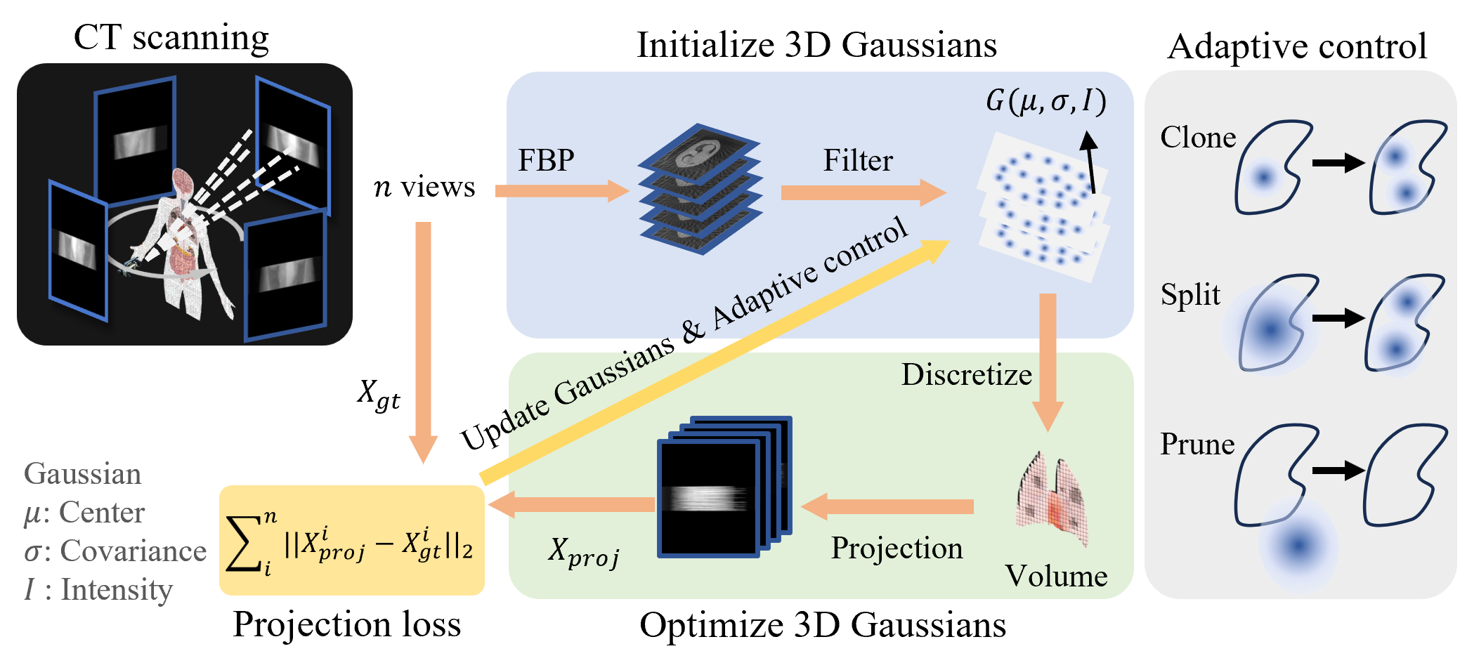
Figure 1: Pipeline Overview: Initially, projection data is acquired from various viewpoints and subsequently processed using Filtered Back Projection (FBP) to yield the FBP-reconstructed image. This reconstructed image is then utilized as a prior for initializing the 3D Gaussians. During the training phase, these 3D Gaussians are discretized into a volumetric image, which then undergoes a forward projection process. We compare the difference between these projections and the ground truth measurements, and use the gradients to update parameters of gaussians. Ultimately, the interplay of the gradient and the Gaussians’ parameters dictates the density control of the Gaussians.

2.1 Initialization of Gaussians

Compared to representing images with neural networks, 3D Gaussians can benefit more from prior information. [7] suggests that an effective initialization for Gaussians can be achieved by utilizing points derived from a structure-from-motion (SfM) process, which involves the correspondence of points across multiple views and the estimation of camera pose. Conversely, the computed tomography (CT) acquisition process provides precise information regarding the radiation source and detectors, thereby rendering the filtered back projection (FBP) method a more suitable technique. To determine the initial positions of the Gaussian centers, an FBP is performed on the acquired projection data $P$. A threshold $\tau$ is applied to exclude empty spaces.

$$I_{FBP}(x,y,z)=\begin{cases}I_{FBP}(x,y,z)&\text{if }I_{FBP}(x,y,z)>\tau,\\ 0&\text{otherwise}\end{cases}$$ (3)

Then we compute the gradient $\nabla I_{FBP}$ of each voxel in the FBP-reconstructed image $I_{FBP}$. We rank the coordinates of these voxels ${V_{i}}$ based on the norm of their gradient $||\nabla I_{FBP}(V_{i})||$. Voxels with very large gradients are usually streaking artifacts in the FBP-reconstructed image. Therefore, we take the coordinates of voxels with medium gradient norms to initialize the Gaussian centers ${C_{j}}$. For each initialized point $C_{j}$, we calculate number of their neighbors $N(C_{j},r)$ within a distance $r$. The radius $\sigma_{j}$ of the Gaussian at $C_{j}$ is set to be inversely proportional to the number of neighbors; and the intensity $I_{j}$ is set to be proportional to the intensity of the FBP-reconstructed image at $C_{j}$.

$$\sigma_{j} =k_{\sigma}\frac{1}{N(C_{j},r)}$$ (4)

$$I_{j} =k_{I}I_{FBP}(C_{j})$$

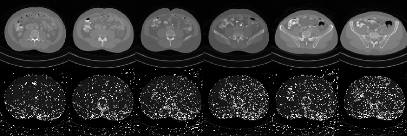
Figure 2: Visualization of the initialized gaussian centers. The initialized position of Gaussians effectively coverage the foreground in the image, and the density of points reflect the complexity of certain region.

2.2 Optimization of Gaussians

To incorporate the 3D Gaussian representation with existing differentiable CT simulators [1], we discretize the Gaussians into a grid of voxels. We optimize this process for efficiency by considering the impact of Gaussians within a specific confidence interval. More precisely, we limit the calculation for each Gaussian $G_{i}$ to the extent defined by $\mu_{i}\pm d$, where $d\geq 3\sigma_{i}$ is a predefined hyperparameter. If a particular Gaussian $G_{i}$ has $\sigma_{i}$ that exceeds $\frac{1}{3}d$ and possesses a high gradient magnitude, we split it into two new Gaussians of smaller radius. This process is further elaborated in Section 2.3. A differentiable CT simulator is used to project the discretized volume. Discrepancies between these projections $\hat{P}$ and the actual measurements $P$ guide the iterative refinement of the Gaussian parameters. We use the L2 norm as a metric to quantify these discrepancies.

$$\centering\min_{\{x_{i},y_{i},z_{i},\Sigma_{i},I_{i}\}_{i=1}^{N}}||\hat{P}(\{x_{i},y_{i},z_{i},\Sigma_{i},I_{i}\}_{i=1}^{N})-P||_{2}^{2}\@add@centering$$ (5)

2.3 Adaptive Density Control

Following [7], we enhance overall accuracy and reconstruction quality through adaptively controlling the density of Gaussians. Different from the original, we consider the gradients of $\mu$ in world space rather than view space. This control mechanism integrates three strategies: cloning, splitting, and pruning. For under-reconstructed spaces, we clone the relevant Gaussian into two copies; for over-reconstructed spaces, we split the relevant Gaussian into two smaller Gaussians. We prune near-zero density or an overly large Gaussians. One of the two cloned Gaussian inherits the gradient and moves along this direction in the following optimization; and its intensity is halved. The split Gaussians maintain a scale proportional to the original. Their positions are initialized by treating the original 3D Gaussian as a Probability Density Function (PDF) from which to sample.

3 Experiments

3.1 Experimental Setup

Datasets and Implementation Details We utilize the "2016 NIH-AAPM-Mayo Clinic Low Dose CT Grand Challenge" dataset [9], including both chest and abdomen CT scans. For each body parts, we use 10 cases. For reconstruction, we assume 20 projections equally distributed across a semicircle which are used to compute cone-beam projections for 3D CT. The scanning geometry implements a cone-beam X-Ray source with a detector composed of $512\times 800$ elements.

The image size used in training after cropping and resizing is 128 $\times$ 128 $\times$ 40, with voxel coordinates normalized to $[0,1]$. Voxel intensities are also normalized to $[0,1]$. For the FBP reconstruction, we apply the Ram-Lak filter with frequency scaling set to 1.0. For training, we use Adam optimizer with ($\beta_{1}$, $\beta_{2}$) = (0.9, 0.999), the learning rate for $\mu$ starts from 2e-4, with an exponential decrease to 2e-6 by the end of the training process. The learning rate for the covariance matrix $\Sigma$ and intensity $I$ is constantly 0.05. The models are trained on a Nvidia 3090 GPU for 30K iterations.

Reconstructed CT images are quantitatively assessed using the structural similarity index metric (SSIM) and peak signal-to-noise ratio (PSNR).

3.2 Main Results

We compare the 3D Gaussian representation with NeRP [13], which represents the image volume using a neural network. Both 3D Gaussian and NeRP are continuous representations. We also list the performance of iterative optimization, which is a discrete representation that takes voxels as the optimization object. The compared NeRP uses an 8-layer MLP, each layer has a width of 256 $\times$ 256.

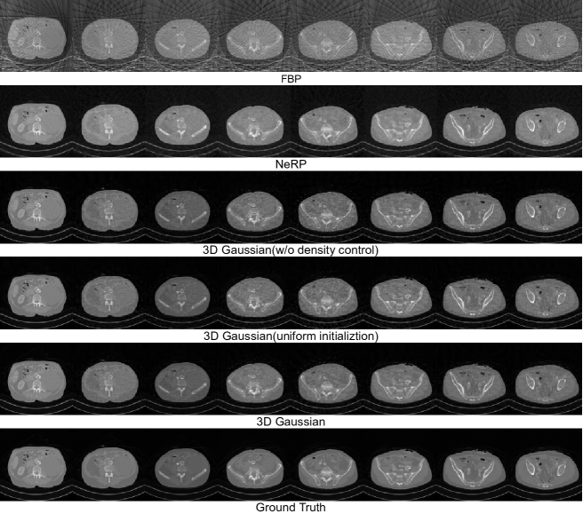
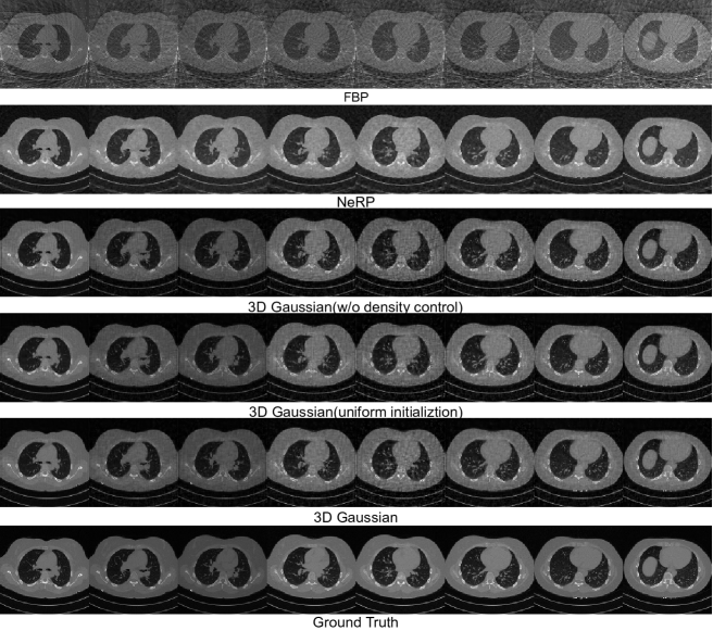
Figure 3: Results of 3D CT image reconstruction for Abdomen CT and Chest CT using 20 projections. The upper is case L506 (abdomen), the bottom is case C295 (chest). Each row show 8 cross-sectional slices of the 3D volume. Results without density control is obtained with 300K Gaussians.

The 3D Gaussian results are obtained with the following setting: Initialize the image with 150K Gaussians, the threshold $\tau$ used to determine emptiness is set to 0.05. The coefficients $k_{\sigma}$ and $k_{I}$ for each Gaussian $G_{i}$ are set to 0.12 and 0.3 for abdominal imaging, and 0.25 and 0.15 for chest imaging, respectively. Density control starts after the first 100 iterations. The maximum permissible gradient norm is set to 1e-5, the minimum intensity of each Gaussian is set to 0.001, and the extent $d$ is set to 0.05. The number of total Gaussians increases with iterations, and we set the maximum number of Gaussians at 400K.

Quantitative results are provided in Table 1, 3D Gaussian achieves superior performance in most cases, usually by a large margin. A visual comparison between images reconstructed using NeRP and 3D Gaussians is shown in Fig. 3. Compared to NeRP, reconstructing images with 3D Gaussians provides cleaner results in empty regions and better high-frequency details like the airways.

Table 1: Quantitative Results on AAPM-Mayo Dataset.

Abdomen	L067		L096		L109		L143		L192		L286		L291		L310		L333		L506		Average
Method	PSNR	SSIM	PSNR	SSIM	PSNR	SSIM	PSNR	SSIM	PSNR	SSIM	PSNR	SSIM	PSNR	SSIM	PSNR	SSIM	PSNR	SSIM	PSNR	SSIM	PSNR	SSIM
FBP	18.48	.625	18.85	.631	18.81	.620	18.86	.590	19.11	.670	18.30	.606	18.15	.608	18.33	.629	19.26	.668	19.78	.690	18.80	.634
Iterative	34.47	.943	35.48	.951	35.03	.948	34.99	.950	35.41	.947	34.78	.948	34.83	.946	36.81	.962	35.02	.945	35.08	.945	35.19	.949
NeRP	34.73	.952	36.91	.968	37.43	.971	36.22	.962	38.59	.978	36.48	.967	36.03	.962	36.42	.967	37.67	.972	36.78	.968	36.73	.967
3D Gaussian (uniform)	37.22	.968	37.58	.971	37.60	.972	35.72	.959	38.30	.976	35.07	.954	35.98	.959	37.61	.972	39.33	.980	39.23	.980	37.37	.969
3D Gaussian	38.59	.976	37.81	.973	39.19	.979	36.58	.966	39.38	.981	36.00	.962	36.25	.962	38.34	.976	40.20	.984	40.64	.984	38.30	.975
Chest	C249		C252		C257		C258		C261		C267		C268		C280		C295		C296		Average
Method	PSNR	SSIM	PSNR	SSIM	PSNR	SSIM	PSNR	SSIM	PSNR	SSIM	PSNR	SSIM	PSNR	SSIM	PSNR	SSIM	PSNR	SSIM	PSNR	SSIM	PSNR	SSIM
FBP	20.80	.637	20.25	.599	19.76	.601	19.08	.603	20.35	.636	18.88	.557	20.65	.620	19.62	.585	19.13	.582	20.22	.626	19.88	.605
Iterative	33.49	.934	32.74	.927	34.58	.946	35.27	.951	33.46	.930	33.60	.938	32.53	.920	34.31	.944	32.56	.922	34.80	.947	33.74	.936
NeRP	35.04	.959	34.91	.956	35.21	.956	34.72	.950	35.18	.959	33.63	.938	34.76	.955	34.54	.946	33.43	.942	35.55	.958	34.70	.952
3D Gaussian (uniform)	35.66	.965	35.13	.960	34.90	.953	34.25	.947	35.93	.964	33.33	.936	35.74	.966	35.05	.954	34.65	.952	35.31	.957	35.00	.956
3D Gaussian	37.37	.976	36.15	.968	35.77	.962	34.91	.955	37.09	.972	34.05	.945	37.30	.975	35.95	.963	35.25	.959	37.15	.972	36.10	.965

3.3 Ablations

We further explore factors that affect the reconstruction quality with 3D Gaussians. This includes examining the number of Gaussians involved and their initialization method, as well as providing evidence of the efficacy of adaptive density control.

3.3.1 Impact of number of gaussians

To understand the number of Gaussians needed to represent an image volume, we turn off the adaptive density control during training, which brings perturbation to the number of Gaussians, and use 10K, 50K, 150K, 300K, 400K, 600K Gaussians to represent a volume. The results are shown in Fig. 4(b) and Fig. 4(c), respectively. The reconstruction performance generally improves with the increase in number of Gaussians used. However, an overly large number of Gaussians can lead to a degraded quality, which may be attributed to the low quality of initialized centers with the increase in number of selected points.

3.3.2 Initialization of Gaussians

We compare our initialization from FBP-reconstructed image strategy with uniform initialization. For uniform initialization, we use the same threshold $\tau$ to filter the air region and initialize the center of Gaussians uniformly across the foreground region, and all Gaussisans are initialized with the same standard deviation and intensity. Quantitative results are listed in Table 1, and visualization is provided in Fig. 3. Initialization from FBP-reconstructed images consistently outperforms uniform initialization by a large margin, suggesting the importance of starting with an informed initial placement of Gaussians.

3.3.3 Effectiveness of Adaptive density control

In our main experiment, we initialize an image with 150K Gaussians and set the upper bound to 400K. Comparisons of reconstruction with and without adaptive density control are provided in Fig. 4(b) and Fig. 4(c). Adaptive density control greatly improves the final reconstruction performance. Moreover, analyzing the correlation between number of Gaussians employed and reconstruction quality reveals that each substantial increase in number of Gaussians corresponds to a temporary drop in reconstruction quality, then recovery and improvement, as depicted in Fig. 4(a). This suggests adaptive density control helps place the Gaussians in a better place compared with solely based on optimization.

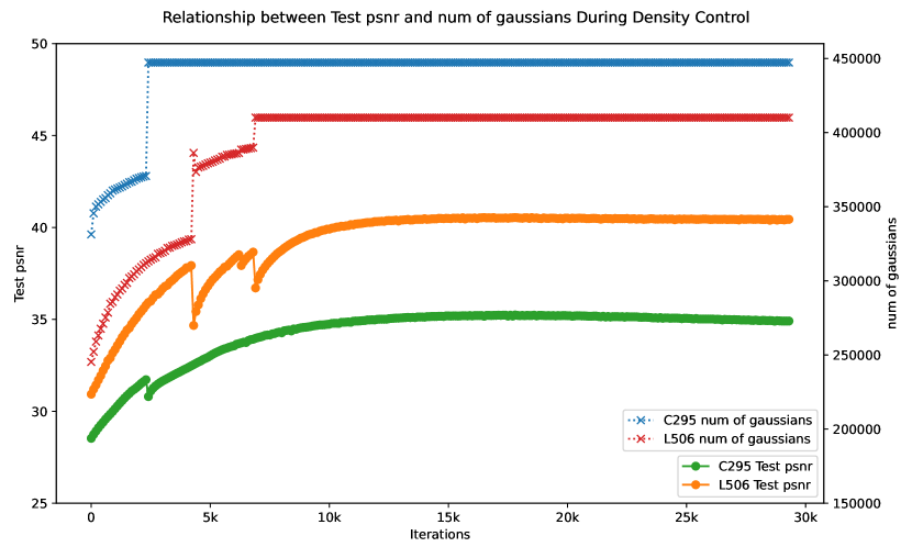
(a)

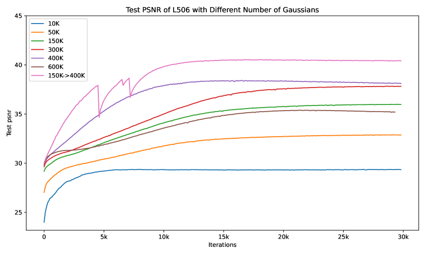
(b)

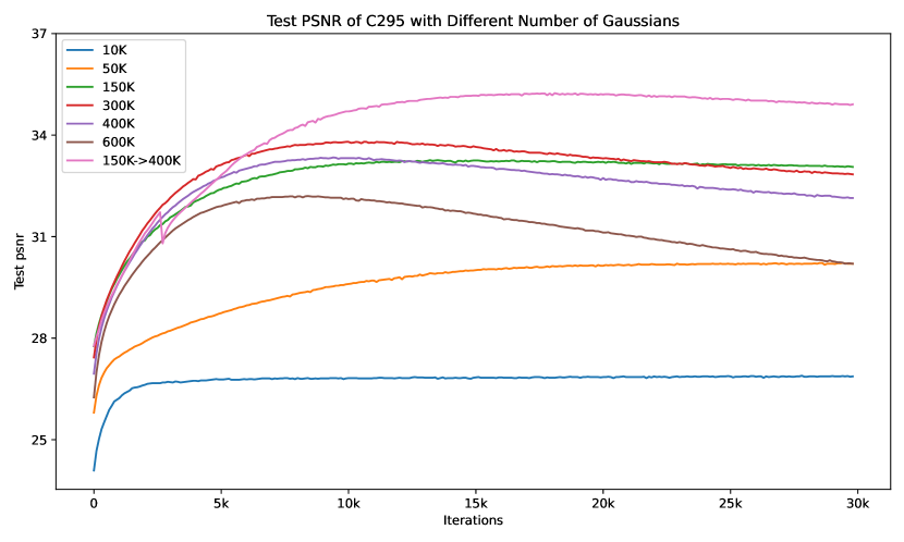
(c)

Figure 4: Ablation studies on number of gaussians and adaptive density control. (a) illustrates the correlation between the reconstruction performance and the number of Gaussians utilized in training with adaptive density control. (b) and (c) compare the reconstruction performance with and without adaptive density control on L506 and C295, respectively, across a range of Gaussian counts.

4 Conclusion

In this paper, we investigate employing 3D Gaussian representation for sparse-view CT reconstruction. We propose to initialize Gaussians based on the FBP-reconstructed image, and perform adaptive density control to enhance the reconstruction quality. These strategies enable 3D Gaussians to effectively reconstruct high-quality 3D images from sparse and noisy data, surpassing the performance of implicit neural representations (INRs)-based methods on the AAPM-Mayo dataset. This innovative methodology incorporates advantages of implicit neural representations, while addressing some of their fundamental limitations, particularly in the context of convergence speed and the handling of high-frequency details. The results highlight the potential of 3D Gaussians in enhancing medical imaging, offering a promising direction to reduce radiation exposure while preserving diagnostic integrity.

References

- [1] Adler, J., Kohr, H., Öktem, O.: Operator discretization library (odl) (Jan 2017). https://doi.org/10.5281/zenodo.249479, https://doi.org/10.5281/zenodo.249479
- [2] Andersen, A.H., Kak, A.C.: Simultaneous algebraic reconstruction technique (sart): a superior implementation of the art algorithm. Ultrasonic imaging 6(1), 81–94 (1984)
- [3] Anirudh, R., Kim, H., Thiagarajan, J.J., Mohan, K.A., Champley, K., Bremer, T.: Lose the views: Limited angle ct reconstruction via implicit sinogram completion. In: Proceedings of the IEEE Conference on Computer Vision and Pattern Recognition. pp. 6343–6352 (2018)
- [4] Bian, J., Siewerdsen, J.H., Han, X., Sidky, E.Y., Prince, J.L., Pelizzari, C.A., Pan, X.: Evaluation of sparse-view reconstruction from flat-panel-detector cone-beam ct. Physics in Medicine & Biology 55(22), 6575 (2010)
- [5] Fang, Y., Mei, L., Li, C., Liu, Y., Wang, W., Cui, Z., Shen, D.: Snaf: Sparse-view cbct reconstruction with neural attenuation fields. arXiv preprint arXiv:2211.17048 (2022)
- [6] Feldkamp, L.A., Davis, L.C., Kress, J.W.: Practical cone-beam algorithm. Josa a 1(6), 612–619 (1984)
- [7] Kerbl, B., Kopanas, G., Leimkühler, T., Drettakis, G.: 3d gaussian splatting for real-time radiance field rendering. ACM Transactions on Graphics (ToG) 42(4), 1–14 (2023)
- [8] Lee, H., Lee, J., Kim, H., Cho, B., Cho, S.: Deep-neural-network-based sinogram synthesis for sparse-view ct image reconstruction. IEEE Transactions on Radiation and Plasma Medical Sciences 3(2), 109–119 (2018)
- [9] McCollough, C., Chen, B., Holmes, D., Duan, X., Yu, Z., Xu, L., Leng, S., Fletcher, J.: Low dose ct image and projection data [data set]. The Cancer Imaging Archive 10 (2020)
- [10] Molaei, A., Aminimehr, A., Tavakoli, A., Kazerouni, A., Azad, B., Azad, R., Merhof, D.: Implicit neural representation in medical imaging: A comparative survey. In: Proceedings of the IEEE/CVF International Conference on Computer Vision. pp. 2381–2391 (2023)
- [11] Müller, T., Evans, A., Schied, C., Keller, A.: Instant neural graphics primitives with a multiresolution hash encoding. ACM Transactions on Graphics (ToG) 41(4), 1–15 (2022)
- [12] Reed, A.W., Kim, H., Anirudh, R., Mohan, K.A., Champley, K., Kang, J., Jayasuriya, S.: Dynamic ct reconstruction from limited views with implicit neural representations and parametric motion fields. In: Proceedings of the IEEE/CVF International Conference on Computer Vision. pp. 2258–2268 (2021)
- [13] Shen, L., Pauly, J., Xing, L.: Nerp: implicit neural representation learning with prior embedding for sparsely sampled image reconstruction. IEEE Transactions on Neural Networks and Learning Systems (2022)
- [14] Sidky, E.Y., Pan, X.: Image reconstruction in circular cone-beam computed tomography by constrained, total-variation minimization. Physics in Medicine & Biology 53(17), 4777 (2008)
- [15] Sun, Y., Liu, J., Xie, M., Wohlberg, B., Kamilov, U.S.: Coil: Coordinate-based internal learning for imaging inverse problems. arXiv preprint arXiv:2102.05181 (2021)
- [16] Tancik, M., Srinivasan, P., Mildenhall, B., Fridovich-Keil, S., Raghavan, N., Singhal, U., Ramamoorthi, R., Barron, J., Ng, R.: Fourier features let networks learn high frequency functions in low dimensional domains. Advances in Neural Information Processing Systems 33, 7537–7547 (2020)
- [17] Wang, C., Shang, K., Zhang, H., Li, Q., Zhou, S.K.: Dudotrans: Dual-domain transformer for sparse-view ct reconstruction. In: International Workshop on Machine Learning for Medical Image Reconstruction. pp. 84–94. Springer (2022)
- [18] Wu, Q., Li, Y., Sun, Y., Zhou, Y., Wei, H., Yu, J., Zhang, Y.: An arbitrary scale super-resolution approach for 3d mr images via implicit neural representation. IEEE Journal of Biomedical and Health Informatics 27(2), 1004–1015 (2022)
- [19] Wu, Q., Li, Y., Xu, L., Feng, R., Wei, H., Yang, Q., Yu, B., Liu, X., Yu, J., Zhang, Y.: Irem: High-resolution magnetic resonance image reconstruction via implicit neural representation. In: Medical Image Computing and Computer Assisted Intervention–MICCAI 2021: 24th International Conference, Strasbourg, France, September 27–October 1, 2021, Proceedings, Part VI 24. pp. 65–74. Springer (2021)
- [20] Zha, R., Zhang, Y., Li, H.: Naf: neural attenuation fields for sparse-view cbct reconstruction. In: International Conference on Medical Image Computing and Computer-Assisted Intervention. pp. 442–452. Springer (2022)
- [21] Zhang, Z., Liang, X., Dong, X., Xie, Y., Cao, G.: A sparse-view ct reconstruction method based on combination of densenet and deconvolution. IEEE transactions on medical imaging 37(6), 1407–1417 (2018)