Gradient Flow Exact Renormalization Group for Scalar Quantum Electrodynamics

Abstract

Gradient Flow Exact Renormalization Group (GF-ERG) is a framework to define the renormalization group flow of Wilsonian effective action utilizing coarse-graining along the diffusion equations. We apply it for Scalar Quantum Electrodynamics and derive flow equations for the Wilsonian effective action with the perturbative expansion in the gauge coupling. We focus on the quantum corrections to the correlation functions up to the second order of the gauge coupling and discuss the gauge invariance of the GF-ERG flow. We demonstrate that the anomalous dimension of the gauge field agrees with the standard perturbative computation and that the mass of the photon keeps vanishing in general spacetime dimensions. The latter is a noteworthy fact that contrasts with the conventional Exact Renormalization Group formalism in which an artificial photon mass proportional to a cutoff scale is induced. Our results imply that the GF-ERG can give a gauge-invariant renormalization group flow in a non-perturbative way.

I Introduction

The Exact Renormalization Group (ERG) Wilson:1973jj ; Polchinski:1983gv ; Wegner:1972ih ; Wetterich:1992yh is a powerful tool for addressing non-perturbative phenomena in quantum field theory Morris:1993qb ; Morris:1998da ; Berges:2000ew ; Aoki:2000wm ; Bagnuls:2000ae ; Polonyi:2001se ; Pawlowski:2005xe ; Gies:2006wv ; Delamotte:2007pf ; Rosten:2010vm ; Kopietz:2010zz ; Braun:2011pp ; Dupuis:2020fhh . In particular, ERG techniques have been employed to explore critical phenomena and phase transitions in strongly correlated systems, such as the Hubbard model in condense-matter physics and quantum chromodynamics in high-energy physics.

The central idea of the ERG is the coarse-graining for quantum fluctuations within the path integral. Integrating out quantum fluctuations with higher momentum $|p|\gtrsim\Lambda$ with an artificial cutoff $\Lambda$ embodies the coarse-graining. This procedure entails the Wilsonian effective action $S_{\Lambda}$, which contains infinite effective operators. In this framework, a functional differential equation describes the change of the effective action $S_{\Lambda}$ induced by quantum fluctuations under the cutoff variation Wilson:1973jj ; Polchinski:1983gv ; Wegner:1972ih ; Wetterich:1992yh and is called “the ERG equation”.

However, the introduction of the explicit momentum cut-off conflictes with gauge symmetries. Since preserving gauge symmetries in describing quantum systems is essential to compute physical quantities, using the ERG tends to be avoided, especially in particle physics. Several attempts Litim:1998wk ; Litim:1998nf ; Morris:2016nda ; Wetterich:2016ewc ; Asnafi:2018pre ; Igarashi:2019gkm ; Igarashi:2021zml ; Igarashi:2016gcf ; Fejos:2016wza ; Fejos:2017sjl have been made to realize a gauge-invariant formulation of non-perturbative renormalization group methods.

The Gradient Flow Exact Renormalization Group (GF-ERG) is a potential framework of the gauge-invariant formulation of the ERG and has recently been suggested in Ref. Sonoda:2020vut . One of its novel features is the incorporation of coarse-graining along the flow of diffusion equations (“gradient flow”) for field operators into the RG flow. From the GF-ERG perspective, the conventional ERG formalism with the exponentially damping UV cutoff function is based on the simple diffusion equation, which does not respect gauge symmetries. One can derive a new type of ERG equation with GF-ERG by replacing this simple diffusion equation with a general one. A unique feature of the GF-ERG formalism is that it can define RG flows that inherit local or global symmetries of the general diffusion equations. Leveraging this attribute allows us to define manifestly gauge-invariant renormalization group flows through GF-ERG.

GF-ERG has been applied in various physical systems, such as pure Yang-Mills theory Sonoda:2020vut , quantum electrodynamics (QED) Miyakawa:2021hcx ; Miyakawa:2021wus , scalar field theory Abe:2022smm , and free Dirac fermions with background gauge fields Miyakawa:2023yob . These studies show that the GF-ERG successfully realizes the invariance of symmetries along renormalization group flows, at least at the perturbative level. In particular, Refs. Miyakawa:2021hcx ; Miyakawa:2021wus have studied QED (describing the interaction between the electrons and the photon) and have shown that the gauge invariance is maintained in the sense that the two-point correlation function of the gauge field satisfies transversality. Furthermore, the counterpart of the ERG equation in the GF-ERG formalism has been derived and called “the GF-ERG equation”. It is a highly non-trivial extension of the ERG equation and involves additional loop corrections from modifying diffusion equations.

Here, we are interested to know whether the GF-ERG formulation realizes the gauge invariance in other systems. Our work aims to explore this point by examining a well-established physical system, namely scalar quantum electrodynamics (sQED). In this paper, we show that the GF-ERG equation yields the transverse kinetic term of the gauge field, that is, $2\gamma_{1}(k^{2}-k^{\mu}k^{\nu})$ with an appropriate anomalous dimension at the perturbative one-loop level $\gamma_{1}=1/48\pi^{2}$ in four dimensions. Furthermore, we also show that the mass of the gauge field is not induced at one-loop level in general dimensions. The latter result contrasts with the conventional ERG equation, which yields a finite gauge field mass proportional to the cutoff scale. These findings indicate that GF-ERG could realize a gauge-invariant formulation for the ERG.

In this study, we work on the following procedures: First, we define the Wilsonian effective action for sQED utilizing GF-ERG and investigate the condition of the BRST invariance of the effective action (or Ward-Takahashi identity). Second, we derive the GF-ERG equations for vertices in the Wilsonian effective action order by order with perturbative expansions in the sQED gauge coupling. Finally, we construct the two-point correlation function of the gauge field from which the anomalous dimension and loop corrections to the mass of the gauge field are read off. In particular, we show that the anomalous dimension agrees with the standard perturbative calculation in four dimensions and that the mass of the gauge field does not receive loop corrections in general dimensions.

This paper is organized as follows. In Section II, we briefly review the conventional formulation of ERG. We also give an alternative definition of the Wilsonian effective action, leading to the idea of GF-ERG. In Section III, we define the Wilsonian effective action for sQED, combining GF-ERG and a set of diffusion equations with BRST invariance. Then we derive the flow equation of the effective action (“GF-ERG equation”) and the Ward-Takahashi identity, which is the result of the manifest gauge invariance [or Becchi-Rouet-Stora-Tyutin (BRST) invariance] of the GF-ERG flow. In Section IV, we solve the GF-ERG equation for sQED perturbatively up to the second order in the gauge coupling. We investigate the one-loop correction to the two-point function of the $U(1)$ gauge field to see that the mass term of the gauge field is not generated in the second-order correction from the matter field. Section V is devoted to conclusions and discussions.

II Wilson-Polchinski equation and diffusion equation

The renormalization group equation is expressed as a functional differential equation whose form is not unique in quantum field theory. In this work, we deal with the Wilson-Polchinski-type equation. This section briefly reviews the conventional Wilson-Polchinski equation Wilson:1973jj ; Polchinski:1983gv to highlight a difference from the GF-ERG equation.

Let us start with the path integral for a scalar field theory described by the bare action $S_{0}[\phi]$ defined on a certain energy scale $\Lambda_{0}$ where the field $\phi$ is a function of momentum $p$. More specifically, the action at $\Lambda_{0}$ is given by

$$S_{0}[\phi]=-\frac{1}{2}\int_{p}\left[\frac{p^{2}}{K(p/\Lambda_{0})}\phi(-p)\phi(p)\right]+S_{0}^{I}[\phi]\,,$$ (1)

where $S_{0}^{I}[\phi]$ is the interaction part of the action and $\int_{p}\mathrel{\mathop{:}}=\int\text{d}^{D}p/(2\pi)^{D}$ is a short-hand notation for the momentum integral in $D$ dimensional spacetime. Here, $K(p/\Lambda_{0})$ is the regulator as a smooth function of $p/\Lambda_{0}$ and behaves as

$$K(p/\Lambda_{0})=\begin{cases}1&\text{for $p\to 0$}\,,\\ 0&\text{for $p\to\infty$}\,.\end{cases}$$ (2)

This implies that the propagator of $\phi$ reads $K(p/\Lambda_{0})/p^{2}$ and thus the theory is regularized in sense that the scalar field for $p>\Lambda_{0}$ does not propagate.

We now divide the momentum into the higher momentum mode $\Lambda\leq|p|\leq\Lambda_{0}$ and the lower one $|p|\leq\Lambda$ by introducing a certain cutoff scale $\Lambda$. This can be implemented by the division of the field such that $\phi(p)=\phi(p)+\varphi(p)$ where

$$\phi(p)=\begin{cases}\phi(p)&\text{$p\leq\Lambda$, otherwise zero};\\[4.30554pt] \varphi(p)&\text{$p>\Lambda$, otherwise zero}.\end{cases}$$ (3)

In the path integral formalism, the path integral measure is divided into $\mathcal{D}\phi=\mathcal{D}\phi\mathcal{D}\varphi$. Then, by integrating out only the higher momentum mode field $\varphi$, we can defines the Wilsonian effective action $S_{\tau}[\phi]$ as

$$e^{S_{\tau}[\phi]}=\int{\mathcal{D}}\varphi\,e^{S_{0}[\phi+\varphi]}\,.$$ (4)

Here, we have introduced the dimensionless scale $\tau-\tau_{0}=\log(\Lambda_{0}/\Lambda)$ so that $S_{\tau_{0}}=S_{0}$.

The Wilson-Polchinski equation describes the change of the Wilsonian effective action $S_{\tau}$ under varying the dimensionless scale $\tau$ (or equivalently $\Lambda$) in a functional differential equation. We hand over its detailed derivation to, e.g. Refs. Wilson:1973jj ; Polchinski:1983gv ; Dutta:2020vqo and show the explicit form of the conventional Wilson-Polchinski equation here. For our purposes, we first define dimensionless quantities with the dimensionless cutoff scale $\Lambda$ such that

$$\tilde{\phi}(\tilde{p})=\Lambda^{d_{\phi}-D}\phi(p)\,, \tilde{p}=p/\Lambda\,,$$ (5)

with $d_{\phi}$ the mass-dimension of the field $\phi$. With these quantities, the Wilson-Polchinski equation is given by

$$\partial_{\tau}e^{S_{\tau}[\tilde{\phi}]} =\int_{\tilde{p}}{\left[\frac{\Delta(\tilde{p})}{K(\tilde{p})}-(d_{\phi}-D)-\gamma_{\phi}+\tilde{p}\cdot\partial_{{\tilde{p}}}\right]\tilde{\phi}(\tilde{p})\cdot\frac{\delta}{\delta\tilde{\phi}(\tilde{p})}e^{S_{\tau}[\tilde{\phi}]}}$$

$$\quad+\int_{\tilde{p}}\left\{\frac{1}{\tilde{p}^{2}}\left[\frac{2\Delta(\tilde{p}){\mathcal{K}}(\tilde{p})}{K(\tilde{p})}+\tilde{p}\cdot\partial_{{\tilde{p}}}{\mathcal{K}}(\tilde{p})\right]-2\gamma_{\phi}\right\}\frac{1}{2}\frac{\delta^{2}}{\delta\tilde{\phi}(\tilde{p})\delta\tilde{\phi}(-\tilde{p})}e^{S_{\tau}[\tilde{\phi}]}\,,$$ (6)

where we have introduced short-hand notations, $\tilde{p}\cdot\partial_{\tilde{p}}=\tilde{p}_{\mu}{\partial}/{\partial\tilde{p}_{\mu}}$ and

$$\Delta(\tilde{p})=\Lambda\frac{\partial}{\partial\Lambda}K(\tilde{p})\,, {\mathcal{K}}(\tilde{p})=K(\tilde{p})\Big{(}1-K(\tilde{p})\Big{)}\,.$$ (7)

and $\gamma_{\phi}$ is the anomalous dimension of $\phi$.

Hereafter, we deal with the dimensionless version of the Wilson-Polchinski equation and, therefore, remove tildes on dimensionless quantities. The Wilson-Polchinski equation (6) for the Wilsonian effective action $S_{\tau}$ is represented schematically in Figure 1. The first term on the right-hand side in Equation 6 is the canonical scaling, while the second term induces quantum corrections. The second-order functional derivative acting on $e^{S_{\tau}[\phi]}$ yields

$$\frac{\delta^{2}}{\delta\phi(p)\delta\phi(-p)}e^{S_{\tau}[\phi]}=e^{S_{\tau}[\phi]}\left[\frac{\delta S_{\tau}[\phi]}{\delta\phi(p)}\frac{\delta S_{\tau}[\phi]}{\delta\phi(-p)}+\frac{\delta^{2}S_{\tau}[\phi]}{\delta\phi(p)\delta\phi(-p)}\right]\,.$$ (8)

Thus, the first term in the square bracket on the right-hand side of this equation corresponds to the dumbbell diagram in Figure 1, while the second term is represented by the ring (loop) diagram. The solid line shows the (modified) propagator given in the bracket $\{~{}\}$ of the second term in Equation 6.

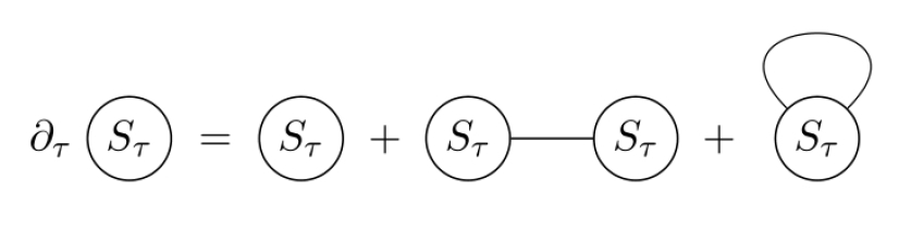
Figure 1: Diagrammatic representation of the conventional Wilson-Polchinski equation (6). The solid line denotes the propagator of the field $\phi$. The first term on the right-hand side corresponds to the canonical scaling due to the introduction of dimensionless quantities. Thus, the second term (the dumbbell diagram) and third term (the ring diagram) corresponds to quantum corrections. The solid line depicts the (modified) propagator.

Now, we intend to formally solve the Wilson-Polchinski equation (6). To this end, let us take the following cutoff function that satisfies Eq. (2):

$$K(p)=e^{-p^{2}}\,.$$ (9)

For this choice, the formal solution to the Wilson-Polchinski equation (6) is found to be Sonoda:2020vut

$$e^{S_{\tau}[\phi]}\mathrel{\mathop{:}}=\hat{s}^{-1}\int{\mathcal{D}}\phi\prod_{x,\mu}\delta\quantity(\phi(x)-e^{-\Theta_{\phi}(\tau)}\phi^{\prime}(t,e^{\tau-\tau_{0}}x))\hat{s}^{\prime}e^{S_{\tau_{0}}[\phi^{\prime}]}\,.$$ (10)

Here, we have introduced the operator

$$\hat{s}\mathrel{\mathop{:}}=\exp(-\frac{1}{2}\int_{p}\frac{\mathcal{K}(p)}{p^{2}}\frac{\delta^{2}}{\delta\phi^{*}(p)\delta\phi(p)})\,,$$ (11)

which is called the “scrambler”, and the scaling factor of $\phi$,

$$\Theta_{\phi}(\tau)=\int^{\tau}_{\tau_{0}}d\tau^{\prime}\quantity(d_{\phi}+\gamma_{\phi}({\tau^{\prime}}))\,.$$ (12)

Equation 10 is can be interpreted as a renormalization transformation from the initial action $S_{\tau_{0}}[\phi^{\prime}]$ to $S_{\tau}[\phi]$. This renormalization transformation naturally entails the flowing field $\phi^{\prime}(t,e^{\tau-\tau_{0}}x)$ with $t-t_{0}=e^{2(\tau-\tau_{0})}-1$, as a solution to the diffusion equation

$$\partial_{t}\phi^{\prime}(t,x)=\partial^{2}\phi^{\prime}(t,x)\,,$$ (13)

with the initial conditions at $t=t_{0}$ (or equivalently $\tau=\tau_{0}$)

$$\phi^{\prime}(t=t_{0},x)=\phi^{\prime}(x)\,.$$ (14)

Therefore, the conventional Wilson-Polchinski equation already involves information on the gradient flow of the field (13). In this sense, GF-ERG can be regarded as an extension of ERG.

III GF-ERG for Scalar QED

In this section, we formulate GF-ERG for sQED following Ref. Sonoda:2020vut . In Section III.1, we introduce the $U(1)$ gauge field, the (anti-)ghost, Nakanishi-Lautrup field and matter scalar field and discuss their diffusion equations which are consistent with the BRST transformation. The right-hand side of equation 13 is not invariant for the gauge (or BRST) transformation, and consequently the conventional Wilson-Polchinski equation is not a gauge-invariant formulation. In the general GF-ERG approach, we deform the simple diffusion equation (13) so that the diffusion equations respect the BRST symmetry. Then, we define the Wilsonian effective action based on these diffusion equations with GF-ERG. In Section III.2, we derive the GF-ERG equation of this Wilsonian effective action, taking the derivative of it with respect to the scale $\tau$. In Section III.3, we study the Gaussian fixed-point action of the GF-ERG equation, which will be used later in performing the perturbative analysis in Section IV. Finally, we investigate the (modified) BRST invariance of the GF-ERG equation and derive the Ward-Takahashi identity for the Wilsonian effective action in Section III.4.

III.1 Definition of Wilsonian effective action

As we have mentioned in Section II, the renormalization transformation for the Wilsonian effective action from $S_{\tau_{0}}$ to $S_{\tau}$ can be expressed as

$$e^{S_{\tau}[\psi]}=\hat{s}^{-1}\int{\mathcal{D}}\psi\prod_{x,\mu}\delta\quantity(\psi(x)-e^{-\Theta_{\psi}(\tau)}\psi^{\prime}(t,e^{\tau-\tau_{0}}x))\hat{s}^{\prime}e^{S_{\tau_{0}}[\psi^{\prime}]}\,.$$ (15)

Note that all quantities and variables are supposed to be dimensionless thanks to the multiplication of an appropriate power of the energy scale $\Lambda$ (See equation 5). Here, $S_{\tau}$ (and $S_{\tau_{0}}$) contains the interactions of the ghost fields $c$, $\bar{c}$ and the Nakanishi-Lautrup field $B$ in addition to the $U(1)$ gauge field $A_{\mu}$ and the complex scalar field $\phi$. For a short-hand notation, we denote the superfield by $\psi$ as $\psi=(A_{\mu},c,\bar{c},B,\phi,\phi^{*})$ in the present system, in which the canonical mass dimensions are given by

$$d_{A}=\frac{D-2}{2}\,, d_{B}=\frac{D}{2}\,, d_{c}=\frac{D-4}{2}\,, d_{\bar{c}}=\frac{D}{2}\,, d_{\phi}=d_{\phi^{*}}=\frac{D-2}{2}\,,$$ (16)

Note that the mass dimensions of the ghost fields are determined from $[\int\text{d}^{D}x\,\bar{c}\,\partial_{\mu}D^{\mu}c]=0$, i.e. $[\bar{c}c]=D-2$ where $[O]$ denotes the mass dimension of the physical quantity $O$. Since the anti-ghost field $\bar{c}$ is not the complex conjugation of the ghost field $c$, but is an independent field of $c$, its mass dimension can be assigned independently. As will be seen later, the assignment for $d_{c}$ and $d_{\bar{c}}$ in Equation 16 is fixed by consistency with the BRST transformation. For the same reason, it turns out that we can set $\gamma_{A}=\gamma_{c}=-\gamma_{\bar{c}}=-\gamma_{B}$ and $\gamma_{\phi}=\gamma_{\phi^{*}}$. The scrambler operator $\hat{s}$ in this system is given by

$$\hat{s}\mathrel{\mathop{:}}=\exp(\int_{p}\left[-\frac{1}{2}\functionalderivative[2]{A_{\mu}(p)}+\frac{1}{2}\functionalderivative[2]{B(p)}+\functionalderivative{c(p)}\functionalderivative{\bar{c}(p)}-\functionalderivative{\phi^{*}(p)}\functionalderivative{\phi(p)}\right])\,.$$ (17)

Here, following Ref. Sonoda:2020vut , we have taken

$$\mathcal{K}(p^{2})=p^{2}\,.$$ (18)

This choice makes the derivation of the GF-ERG equation simple, but does not agree with the Wilson-Polchinski convention (7) with the choice of $K(p)$ as given in Equation 9. The consistency of this choice of $\mathcal{K}(p^{2})$ as a UV cutoff function will be discussed in Section III.3.

The Wilsonian effective action $S_{\tau}$ obtained from Equation 15 with the simple diffusion equations (13) becomes equivalent to the solution to the conventional Wilson-Polchinski equation with cutoff functions (9) and (7). However, these diffusion equations are not invariant under the following BRST transformation:

$${\mbox{\boldmath$\delta$}}_{\rm B}A_{\mu}=\partial_{\mu}c\,, {\mbox{\boldmath$\delta$}}_{\rm B}c=0\,, {\mbox{\boldmath$\delta$}}_{\rm B}\bar{c}=B\,, {\mbox{\boldmath$\delta$}}_{\rm B}\phi=ie_{0}c\phi\,, {\mbox{\boldmath$\delta$}}_{\rm B}B=0\,.$$ (20)

In this sense, the conventional Wilson-Polchinski equation is not BRST (gauge) invariant. Alternately, the BRST invariance under Equation 20 suggests the modification of the diffusion equations for $\phi^{\prime}$ and $\phi^{\prime*}$:

$$\partial_{t}\phi^{\prime}(t,x)=D^{\prime}{}^{2}\phi^{\prime}(t,x)+ie_{0}\partial_{\mu}A^{\prime}_{\mu}(t,x)\phi^{\prime}(t,x)\,,$$ (21a)

$$\partial_{t}{\phi^{\prime}}^{*}(t,x)={D^{\prime}}^{*2}{\phi^{\prime}}^{*}(t,x)-ie_{0}\partial_{\mu}A^{\prime}_{\mu}(t,x){\phi^{\prime}}^{*}(t,x)\,,$$ (21b)

where $D^{\prime}_{\mu}\mathrel{\mathop{:}}=\partial_{\mu}-ie_{0}A^{\prime}_{\mu}(t,x)$. The other fields obey the simple diffusion equations (13) in the same way as the conventional ERG. It should be emphasized here that the above diffusion equations and the covariant derivative $D^{\prime}_{\mu}$ are defined with the bare electric charge $e_{0}$. This BRST invariance is inherited by (the flow of) the Wilsonian effective action, as will be seen in the next subsection. The modified diffusion equations enforce the consistency with the BRST transformation on the fields at an arbitrary energy scale, and thus guarantee the BRST invariance of the system under the RG transformations.

Here, we explain the relation between the anomalous dimensions. If the RG flow is invariant under the BRST transformation, the anomalous dimensions of $A_{\mu}$ and $c$ must agree with each other from Equation 20. For the same reason, we find $\gamma_{\bar{c}}=\gamma_{\bar{B}}$. Also, because the ghost sector in sQED is free, we expect that the ghost term does not receive the wave function renormalization. Therefore, we find $\gamma_{c}=-\gamma_{\bar{c}}$, which leads to $\gamma_{A}=\gamma_{c}=-\gamma_{\bar{c}}=-\gamma_{B}$. For the anomalous dimension of the matter field, the hermiticity of the action gives $\gamma_{\phi}=\gamma_{\phi^{*}}$.

III.2 GF-ERG equation

Now, we derive the GF-ERG equation from Equation 15 and Equation 21. Differentiating the effective action $S_{\tau}$ with respect to $\tau$, we get

$$\partial_{\tau}e^{S_{\tau}} =(\text{R.H.S. of \lx@cref{creftype~refnum}{eq: dimensionless Wilson-Polchinski equation}})+\Bigg{[}4ie_{\tau}\int_{x}\,\widehat{A}_{\mu}(x)\left(\partial_{\mu}+\frac{i}{2}e_{\tau}\widehat{A}_{\mu}(x)\right)\functionalderivative{\phi^{*}(x)}\left(\widehat{\phi}^{*}(x)e^{S_{\tau}}\right)+(\text{c.c})\Bigg{]}\,.$$ (22)

Here, the first terms on the right-hand side are the same as the conventional Wilson-Polchinski equation (6), while the last term arises from the modification of the diffusion equations from Equation 13 to Equation 21. We have introduced the new field operators, $\widehat{A}_{\mu}(x)$, $\widehat{\phi}(x)$ and $\widehat{\phi}^{*}(x)$, which are obtained from the Fourier transformations for the field operators in momentum space:

$$\widehat{A}_{\mu}(p)=\hat{s}^{-1}A_{\mu}(p)\hat{s}=A_{\mu}(p)+\frac{\delta}{\delta A_{\mu}(p)}\,,$$ (23)

$$\widehat{\phi}(p)=\hat{s}^{-1}\phi(p)\hat{s}={\phi}(p)+\frac{\delta}{\delta{\phi}^{*}(p)}\,,$$ (24)

$$\widehat{\phi}^{*}(p)=\hat{s}^{-1}\phi^{*}(p)\hat{s}={\phi}^{*}(p)+\frac{\delta}{\delta{\phi}(p)}.$$ (25)

These terms contain the functional derivatives acting on $S_{\tau}$ and thus induce a number of interacting terms, e.g., $e^{-S_{\tau}}\widehat{A}_{\mu}e^{S_{\tau}}=A_{\mu}+e_{\tau}\phi^{*}\partial_{\mu}\phi+\cdots$. Since the complete GF-ERG equation (22) is quite lengthy, it will be put in Appendix B. In the GF-ERG equation 22, the renormalized electric charge $e_{\tau}$ is defined by

$$e_{\tau} =e_{0}\exp(-\int_{\tau_{0}}^{\tau}\text{d}\tau^{\prime}\,\quantity(\frac{D-4}{2}+\gamma_{A}(\tau^{\prime})))\,.$$ (26)

Whereas the conventional Wilson-Polchinski equation has tree- and one-loop structures, the GF-ERG contains higher loop terms originating from the modification of the diffusion equations. In Section IV, we will derive the flow equations in terms of the perturbative expansion of $e_{\tau}$.

We note here that the GF-ERG equation, in this way, may be regarded as a class of the Wegner equation Wegner:1976bn ; Latorre:2000qc ,

$$\partial_{\tau}e^{S_{\tau}[\phi]}=\int_{x}\frac{\delta}{\delta\phi(x)}\left(\Psi(x)e^{S_{\tau}[\phi]}\right)\,.$$ (27)

Here, $\Psi(x)$ is the general “coarse-graining operator”. The conventional Wilson-Polchinski equation is reproduced by taking

$$\Psi(x)e^{S_{\tau}[\phi]}=\int\mathcal{D}\phi\,\delta(\phi-b_{\tau}[\phi])(\partial_{\tau}b_{\tau}[\phi])e^{S_{0}[\phi]}\,,$$ (28)

where $b_{\tau}[\phi]$ is the coarse-grained effective field as analogous to block-spin transformed variables in spin systems. In other words, this is the definition of $\Phi$ from $\Phi$ as given in Equation 3. For a general GF-ERG equation, one can derive the explicit form of the coarse-graining operator $\Psi(x)$; however, it is complicated, so we do not specify it here and discuss it in Appendix B.

One of the main purposes of this study is to obtain the beta function by using the GF-ERG equation by means of perturbative expansion. To this end, we generalize $\phi\to\Phi=(A_{\mu},B,\bar{c},c,\phi,\phi^{*})$, and divide the fields $\Phi$ into certain background fields $\bar{\Phi}$ and fluctuation fields $\Phi$ such that

$$S_{\tau}[\Phi]=S^{(0)}[\bar{\Phi}]+S^{(1)}[\bar{\Phi}]\Phi+\frac{1}{2!}S^{(2)}[\bar{\Phi}]\Phi^{2}+\frac{1}{3!}S^{(3)}[\bar{\Phi}]\Phi^{3}++\frac{1}{3!}S^{(4)}[\bar{\Phi}]\Phi^{4}+\cdots\,,$$ (29)

where we have omitted the spacetime integrals. The expansion allows us to write the GF-ERG equation (22) in coupled functional differential equations for effective vertices $S^{(n)}[\bar{\Phi}]$ depending on the background field and external momenta. The first term on the right-hand side provides the effective potential $V_{\rm ell}(\bar{\Phi})$ for the background field $\bar{\Phi}$. Therefore, the minimum of $V_{\rm ell}(\bar{\Phi})$ determines the vacuum of the system. In this work, we assume that the symmetric vacuum, i.e. $\bar{\Phi}=0$, is realized. The choice of an appropriate background (vacuum) should involve the equations of motion for the background fields $S^{(1)}[\bar{\Phi}]=0$, so that the second term vanishes. In this work, we deal only with $S^{(2)}[\bar{\Phi}]$, $S^{(3)}[\bar{\Phi}]$ and $S^{(4)}[\bar{\Phi}]$ and truncate the higher-order terms $S^{(n)}[\bar{\Phi}]$ ($n\geq 5$). In the following, we construct the effective propagators $S^{(2)}[\bar{\Phi}]$ and effective vertices ($S^{(3)}[\bar{\Phi}]$, $S^{(4)}[\bar{\Phi}]$) by the GF-ERG.

III.3 Construction of Gaussian part

To construct the Ward-Takahashi identity and perform the perturbative analysis of sQED with GF-ERG, we have to define the tree-level action, i.e. the Gaussian part of the action denoted by $\mathcal{S}_{0}^{(2)}$. We briefly explain how to obtain the Gaussian action in the following. First, we assume that the Gaussian action is $\tau$-independent and has a quadratic form in terms of the original fields $(A_{\mu},B,\bar{c},c,\phi,\phi^{*})$ as

$$\mathcal{S}_{0}^{(2)}\mathrel{\mathop{:}}=\int_{k}\biggl{[}-\frac{1}{2}A_{\mu}(k)\Big{(}S_{0}^{AA}(k)\Big{)}_{\mu\nu}A_{\nu}(-k)-ik_{\mu}A_{\mu}(k)S_{0}^{AB}(k)B(-k)+\frac{1}{2}B(k)S_{0}^{BB}(k)B(-k)\\ -\bar{c}(k)S_{0}^{\bar{c}c}(k)c(-k)-\phi^{*}(k)S_{0}^{\phi^{*}\phi}(k)\phi(-k)\biggr{]}\,.$$ (30)

Then, the solution to GF-ERG equation 22 under the above ansatz yields the explicit forms of the operators $S_{0}^{(2)}(k)$ in terms of the original fields $(A_{\mu},B,\bar{c},c,\phi)$.

Next, we define the “$-1$ variables” Miyakawa:2023yob as

$$\mathcal{A}_{\mu}(k) \mathrel{\mathop{:}}=e^{k^{2}}e^{-S_{0}}\hat{s}^{-1}A_{\mu}(k)\hat{s}e^{S_{0}}=e^{-k^{2}}\left(h_{\mu\nu}(k)A_{\nu}(k)+ik_{\mu}h_{B}(k^{2})B(k)\right)\,,$$ (31a)

$$\mathcal{B}(k) \mathrel{\mathop{:}}=e^{k^{2}}e^{-S_{0}}\hat{s}^{-1}B(k)\hat{s}e^{S_{0}}=e^{-k^{2}}h_{B}(k^{2})\left(B(k)+e^{2k^{2}}ik_{\mu}A_{\mu}(k)\right)\,,$$ (31b)

$$\overline{C}(k) \mathrel{\mathop{:}}=e^{k^{2}}e^{-S_{0}}\hat{s}^{-1}\bar{c}(k)\hat{s}e^{S_{0}}=e^{-k^{2}}h_{S}(k^{2})\overline{c}\,,$$ (31c)

$$C(k) \mathrel{\mathop{:}}=e^{k^{2}}e^{-S_{0}}\hat{s}^{-1}c(k)\hat{s}e^{S_{0}}=e^{-k^{2}}h_{S}(k^{2})c\,,$$ (31d)

$$\Phi(k) \mathrel{\mathop{:}}=e^{k^{2}}e^{-S_{0}}\hat{s}^{-1}\phi(k)\hat{s}e^{S_{0}}=e^{-k^{2}}h_{S}(k^{2})\phi\,.$$ (31e)

These variables play an important role as fundamental variables in the perturbative expansion performed later. Here, we have defined the perturbative propagators $(h_{\mu\nu}(k),h_{B}(k^{2}),h_{S}(k^{2}))$ of the fields as

$$h_{\mu\nu}(k) \mathrel{\mathop{:}}=h_{S}(k^{2})T_{\mu\nu}(k)+\left(\xi+e^{-2k^{2}}\right)h_{B}(k^{2})L_{\mu\nu}(k)\,,$$ (32)

$$h_{B}(k^{2}) \mathrel{\mathop{:}}=\frac{1}{k^{2}+\xi e^{-2k^{2}}+e^{-4k^{2}}}\,,$$ (33)

$$h_{S}(k^{2}) \eqqcolon\frac{1}{k^{2}+e^{-2k^{2}}}\,,$$ (34)

where the gauge fixing parameter $\xi$ is an arbitrary real number and the transverse and longitudinal operators $T_{\mu\nu}(k),L_{\mu\nu}(k)$ are defined as,

$$T_{\mu\nu}(k)\mathrel{\mathop{:}}=\delta_{\mu\nu}-\frac{k_{\mu}k_{\nu}}{k^{2}}\,,\quad L_{\mu\nu}(k)\mathrel{\mathop{:}}=\frac{k_{\mu}k_{\nu}}{k^{2}}\,.$$ (35)

Finally, we rewrite equation 30 in terms of the $-1$ variables (31) to obtain

$$\mathcal{S}_{0}^{(2)}=\int_{k}\biggl{[}-\frac{1}{2}\mathcal{A}_{\mu}(k)\Big{(}S_{0}^{\mathcal{A}\mathcal{A}}(k)\Big{)}_{\mu\nu}\mathcal{A}_{\nu}(-k)-ik_{\mu}\mathcal{A}_{\mu}(k)S_{0}^{\mathcal{A}\mathcal{B}}(k)\mathcal{B}(-k)+\frac{1}{2}\mathcal{B}(k)S_{0}^{\mathcal{B}\mathcal{B}}(k)\mathcal{B}(-k)\\ -\overline{C}(k)S_{0}^{\overline{C}C}(k)C(-k)-\Phi^{*}(k)S_{0}^{\Phi^{*}\Phi}(k)\Phi(-k)\biggr{]}\,,$$ (36)

where the operators $S_{0}^{(2)}(k)$ are given by

$$S_{0}^{\mathcal{A}\mathcal{A}}(k) =\vbox{\hbox{\includegraphics[width=71.13188pt]{TwoPointZeroth_A.JPG}}}=k^{2}\quantity(1+k^{2}e^{2k^{2}})T_{\mu\nu}(k)-k^{2}e^{2k^{2}}L_{\mu\nu}(k)\,,$$ (37a)

$$S_{0}^{\mathcal{A}\mathcal{B}}(k) =\vbox{\hbox{\includegraphics[width=71.13188pt]{TwoPointZeroth_AB.JPG}}}=1+\xi e^{2k^{2}}\,,$$ (37b)

$$S_{0}^{\mathcal{B}\mathcal{B}}(k) =\vbox{\hbox{\includegraphics[width=71.13188pt]{TwoPointZeroth_B.JPG}}}=\xi+(\xi^{2}-k^{2})e^{2k^{2}}\,,$$ (37c)

$$S_{0}^{\Phi^{*}\Phi}(k) =\vbox{\hbox{\includegraphics[width=71.13188pt]{TwoPointZeroth_Phi.JPG}}}=k^{2}\quantity(1+k^{2}e^{2k^{2}}),$$ (37d)

$$S_{0}^{\overline{C}C}(k) =\vbox{\hbox{\includegraphics[width=71.13188pt]{TwoPointZeroth_C.JPG}}}=k^{2}\quantity(1+k^{2}e^{2k^{2}})\,.$$ (37e)

Here, we discuss the consistency of the choice (18) for $\mathcal{K}(p^{2})$ as an ultraviolet (UV) cutoff function. It should be noted that $h_{S}(k^{2})$ plays the role of the loop propagator of the matter field in the following perturbative analysis, whose momentum dependence is depicted in Figure 2. There is no large difference in the qualitative behaviors of the regulated propagator between the choice (18) and equation 7 with the choice (9). Therefore, the choice (18) can be regarded reliable for playing a role as a UV cutoff function, at least at the level of perturbative analysis.

Also, we discuss here gauge-fixing of the action. Because this Gaussian action is a fixed point of the GF-ERG equation with $e_{\tau}=0$, we can take the continuum limit ($\Lambda_{0}\to\infty$). After the limit, we get

$$S_{0}\to S_{G}\mathrel{\mathop{:}}=\int_{k}\biggl{[}-\frac{1}{2}A_{\mu}(k)\quantity(k^{2}T_{\mu\nu}(k)+\frac{k^{2}}{1+\xi}L_{\mu\nu}(k))A_{\nu}(k)-\frac{1}{1+\xi}B(-k)ik_{\mu}A_{\mu}(k)+\frac{\xi}{2(1+\xi)}B(-k)B(k)\\ -\bar{c}(-k)k^{2}c(k)-\phi^{*}(k)k^{2}\phi(k)\biggr{]},$$ (38)

which is expressed in the coordinate space as

$$S_{G}=\int_{x}\biggl{[}-\frac{1}{4}F_{\mu\nu}(x)F_{\mu\nu}(x)-\frac{1}{2(1+\xi)}(\partial_{\mu}A_{\mu}(x))^{2}-\frac{1}{1+\xi}B(x)\partial_{\mu}A_{\mu}(x)+\frac{\xi}{2(1+\xi)}B(x)B(x)\\ -\partial_{\mu}\bar{c}(x)\partial_{\mu}c(x)-\partial_{\mu}\phi^{*}(x)\partial_{\mu}\phi(x)\biggr{]}.$$ (39)

If we integrate out the NL field $B$, we get

$$S_{G}\to\int_{x}\biggl{[}-\frac{1}{4}F_{\mu\nu}(x)F_{\mu\nu}(x)-\frac{1}{2\xi}(\partial_{\mu}A_{\mu}(x))^{2}-\partial_{\mu}\bar{c}(x)\partial_{\mu}c(x)-\partial_{\mu}\phi^{*}(x)\partial_{\mu}\phi(x)\biggr{]},$$ (40)

which agrees with the the continuum sQED action in the $R_{\xi}$ gauge. Therefore, we can consider Equation 30 or Equation 36 as the free sQED action in the $R_{\xi}$ gauge modified by introducing the UV cutoff.

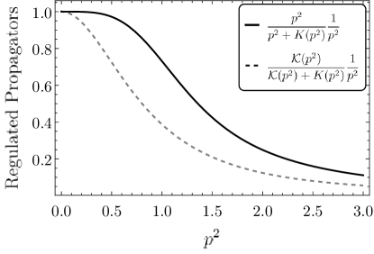
Figure 2: Comparison of the regulated propagators between $\mathcal{K}(p^{2})=p^{2}$ (solid line) and equation 7 with $K(p^{2})=e^{-p^{2}}$ (dashed line).

III.4 Ward-Takahashi identity

We discuss the Ward-Takahashi identities here before deriving the flow equations for the effective vertices $S_{\tau}^{(n)}$ from the GF-ERG equation (22) within the perturbative expansion. In the conventional Wilson-Polchinski equation, there are two origins of the breaking of BRST symmetry: One is the diffusion equation for the fields and the other originates from the scrambler operator $\hat{s}$. The former can be solved by modifying the diffusion equations to Equation 21, as was discussed in Section III.1. Indeed, the latter makes the GF-ERG equation (22) non-invariant under the original BRST transformation (20), which is generated by

$$\hat{\mathcal{G}}_{B}\mathrel{\mathop{:}}=\int_{p}\biggl{[}ip_{\mu}c(p)\functionalderivative{A_{\mu}(p)}+B(p)\functionalderivative{\bar{c}(p)}+ie_{\tau}c(p)\phi(p)\functionalderivative{\phi(p)}-ie_{\tau}c(p)\phi^{*}(p)\functionalderivative{\phi^{*}(p)}\biggr{]}\,.$$ (41)

This is because the scrambler operator is not commutative with this BRST generator, i.e. $[\hat{s},\hat{\mathcal{G}}_{B}]\neq 0$. Instead, following Miyakawa:2021wus ; Miyakawa:2021hcx , we can show that the GF-ERG equation (22) is invariant under the modified BRST transformation, whose generator reads

$$\tilde{\hat{\mathcal{G}}}_{B} \mathrel{\mathop{:}}=\hat{s}\hat{\mathcal{G}}_{B}\hat{s}^{-1}=\int_{p}\biggl{[}\partial_{\mu}\widehat{c}(p)\functionalderivative{A_{\mu}(p)}+\widehat{B}(p)\functionalderivative{\bar{c}(p)}+ie_{\tau}\widehat{c}(p)\phi(p)\functionalderivative{\phi(p)}-ie_{\tau}\widehat{c}(p)\phi^{*}(p)\functionalderivative{\phi^{*}(p)}\biggr{]}\,,$$ (42)

where the fields with hat are defined as

$$\widehat{c}(p)=c(p)+\functionalderivative{\bar{c}(p)}\,, \widehat{\bar{c}}(x)=\bar{c}(p)-\functionalderivative{c(p)}\,, \widehat{B}(p)=B(p)-\functionalderivative{B(p)}\,.$$ (43)

The invariance of the system under the (modified) BRST transformation (42) leads to the modified Ward-Takahashi (WT) identities for the effective vertices $S^{(n)}_{\tau}$. The explicit form of the modified WT identities is lengthy, so we give them in Appendix D. In the next section, we employ the perturbative analysis in the polynomial of $e_{\tau}$ on the effective vertices. In such a case, the Ward-Takahashi identity for the Wilsonian effective action is reduced to

$$e^{k^{2}}k_{\mu}\frac{\delta(S_{\tau}-\mathcal{S}^{(2)}_{0})}{\delta\mathcal{A}_{\mu}(k)}+e_{\tau}\int_{p}\quantity(\phi(p)\functionalderivative{S_{\tau}}{\phi(p+k)}-\phi^{*}(p)\functionalderivative{S_{\tau}}{\phi^{*}(p+k)})=0,$$ (44)

where $\mathcal{S}_{0}^{(2)}$ is the Gaussian part (tree-level part of the Wilsonian effective action $S_{\tau}$) defined in Equation 36. The detailed discussion is given in Appendix D. Note that in equation 44, the first term is given by the functional derivative with respect to the $-1$ variable ($\mathcal{A}_{\mu}$), while the second and third terms are given with the original fields ($\phi$ and $\phi^{*}$).

IV Perturbative analysis of GF-ERG equation

In this section, we intend to solve the GF-ERG equation equation 22 using perturbation theory. To this end, we suppose here that the $n$-point correlation functions $S^{(n)}_{\tau}$ are functions of solely the renormalized charged coupling $e_{\tau}$, and thus $S^{(n)}_{\tau}$ are expanded into the polynomial of $e_{\tau}$ as

$$S^{(n)}_{\tau} =\sum_{l=0}^{\infty}(e_{\tau})^{l}S^{(n)}_{l}=S^{(n)}_{0}+e_{\tau}S^{(n)}_{1}+e_{\tau}^{2}S^{(n)}_{2}+\cdots\,.$$ (45)

Furthermore, assuming that the explicit dependence of $\tau$ on $S^{(n)}_{\tau}$ is given only in the coupling $e_{\tau}$, the left-hand side of equation 22 can be rewritten in terms of the change of $e_{\tau}$ such that

$$\partial_{\tau}S_{\tau} =\partial_{\tau}e_{\tau}\frac{\partial S_{\tau}}{\partial e_{\tau}}=\left[\frac{4-D}{2}-\gamma_{A}(\tau)\right]e_{\tau}\frac{\partial S_{\tau}}{\partial e_{\tau}}\,,$$ (46)

where we have used the renormalization group equation for $e_{\tau}$:

$$\partial_{\tau}e_{\tau}=\left[\frac{4-D}{2}-\gamma_{A}(\tau)\right]e_{\tau}\,,$$ (47)

which follows from the definition (Equation 26) of the renormalized charge $e_{\tau}$.

Then, we evaluate the GF-ERG equation for each vertex order by order of $e_{\tau}$. In this work, we consider the quantum corrections up to the second order of $e_{\tau}$. We focus on the two-point correlation function for the gauge fields and compute $O(e_{\tau}^{2})$ to it. On the other hand, we just consider the Gaussian part for the other fields: that is, the zeroth order of $e_{\tau}$ is considered. Furthermore, we do not consider the $(\phi^{*}\phi)^{2}$-vertex and two-point function of $\phi\phi^{*}$ on the order of $e_{\tau}^{2}$. More specifically, we assume the following ansatz for Wilsonian effective action $S_{\tau}$:

$$S_{\tau}={\mathcal{S}}_{0}^{(2)}+\int_{p,k}\Phi^{*}(p+k)\Phi(p)\left(e_{\tau}S^{\Phi^{*}\Phi\mathcal{A}}_{1}(p,k)\right)_{\mu}\mathcal{A}_{\mu}(k)\\ +\int_{p,k,l}\Phi^{*}(p+k+l)\Phi(p)\mathcal{A}_{\mu}(k)\left(e_{\tau}^{2}S_{2}^{\Phi^{*}\Phi\mathcal{A}\mathcal{A}}(p,k,l)\right)_{\mu\nu}\mathcal{A}_{\nu}(l)+\int_{k}\frac{1}{2}\mathcal{A}_{\mu}(k)\Big{(}e_{\tau}^{2}S_{2}^{\mathcal{A}\mathcal{A}}(k)\Big{)}_{\mu\nu}\mathcal{A}_{\nu}(-k)\,,$$ (48)

where ${\mathcal{S}}_{0}^{(2)}$ is the Gaussian part given in Equation 36. This ansatz is minimal for computing the quantum corrections to the two-point function of the gauge fields at the second order because the other terms do not contribute to it at this order. In the following, we construct $S_{l}^{(n)}$ order by order in the Wilsonian effective action (48).

IV.1 First order $O(e_{\tau})$

We next deal with the solution of the GF-ERG equation at the first order of $e_{\tau}$, i.e. $S^{\Phi^{*}\Phi\mathcal{A}}_{1}(p,k)$ in Equation 48:

$$\mathcal{S}_{1}^{\Phi^{*}\Phi\mathcal{A}}\mathrel{\mathop{:}}=\int_{p,k}{\Phi}^{*}(p+k){\Phi}(p)\left(e_{\tau}S^{\Phi^{*}\Phi\mathcal{A}}_{1}(p,k)\right)_{\mu}{\mathcal{A}}_{\mu}(k)\,.$$ (49)

In terms of $\Phi$, $\Phi^{*}$ and $\mathcal{A}_{\mu}$ as given in Equation 31, the term $\mathcal{S}_{1}^{\Phi^{*}\Phi\mathcal{A}}$ in Equation 45 obeys

$$-\frac{D-4}{2}\mathcal{S}^{\Phi^{*}\Phi\mathcal{A}}_{1}-\int_{k}\Biggl{[}\quantity(k\cdot\partial_{k}+\frac{D+2}{2})\mathcal{A}_{\mu}(k)\cdot\functionalderivative{\mathcal{S}^{\Phi^{*}\Phi\mathcal{A}}_{1}}{\mathcal{A}_{\mu}(k)}+\Biggl{(}\quantity(k\cdot\partial_{k}+\frac{D+2}{2})\Phi(k)\cdot\functionalderivative{\mathcal{S}^{\Phi^{*}\Phi\mathcal{A}}_{1}}{\Phi(k)}+\text{(c.c.)}\Biggr{)}\Biggr{]}\\ =4\int_{p,k}\,\quantity(e^{p^{2}-(p+k)^{2}-k^{2}}p^{2}(p+k)_{\mu}+e^{(p+k)^{2}-p^{2}-k^{2}}(p+k)^{2}p_{\mu})\Phi^{*}(p+k)\mathcal{A}_{\mu}(k)\Phi(p)\,.$$ (50)

The anomalous dimensions of $\mathcal{A}_{\mu}$ and $\Phi$, denoted respectively by $\gamma_{A}$ and $\gamma_{\phi}$, are assumed to be of order of $e_{\tau}^{2}$, so that those are neglected here in $\mathcal{S}^{\Phi^{*}\Phi\mathcal{A}}_{1}$. Note that the first two terms on the right-hand side of Equation 50 exist in the conventional Wilson-Polchinski equation, while the last term arises from modification of the gradient flow equations.

Substituting the ansatz Equation 49 for $\mathcal{S}^{\Phi^{*}\Phi\mathcal{A}}_{1}$ into Equation 50, we obtain the equation for the vertex $(S^{\Phi^{*}\Phi\mathcal{A}}_{1}(p,k))_{\mu}$ such that

$$\quantity(p\cdot\partial_{p}+k\cdot\partial_{k}-1)\left(S^{\Phi^{*}\Phi\mathcal{A}}_{1}(p,k)\right)_{\mu}=4\biggl{(}e^{p^{2}-(p+k)^{2}-k^{2}}p^{2}(p+k)_{\mu}+e^{(p+k)^{2}-p^{2}-k^{2}}(p+k)^{2}p_{\mu}\biggr{)}\,.$$ (51)

The left- and right- hand sides of Equation 51 correspond to those of Equation 50, respectively. We show the diagrammatic expression for Equation 51 in Figure 3.

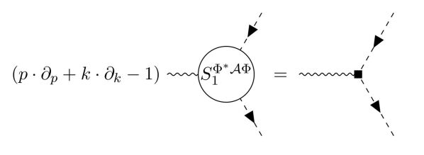
Figure 3: Diagrammatic representation of the GF-ERG equation for $(S_{1}^{\Phi^{*}\Phi\mathcal{A}})_{\mu}$ given in equation 51. The wiggly line represents the propagator of the gauge field $A_{\mu}$, while the complex scalar fields are shown by the dashed line with an arrow. The first two terms on the right-hand side are involved in the conventional Wilson-Polchinski equation, while the others originate from modification of the diffusion equation (21). The black circle and square dots represent the additional vertices that arise from interactions in the modified diffusion equation (21) or, equivalently, the last term in the GF-ERG (22).

Using the formula in Appdix A in Miyakawa:2021wus , the general solution to equation 51 is found to be

$$\left(S^{\Phi^{*}\Phi\mathcal{A}}_{1}(p,k)\right)_{\mu}=ap_{\mu}+bk_{\mu}+2\biggl{(}F(p^{2}-(p+k)^{2}-k^{2})p^{2}(p+k)_{\mu}+F((p+k)^{2}-p^{2}-k^{2})(p+k)^{2}p_{\mu}\biggr{)}\,,$$ (52)

where $a$ and $b$ are arbitrary constants, and we have introduced a function

$$F(x)\mathrel{\mathop{:}}=\frac{e^{x}-1}{x}\,.$$ (53)

The Ward-Takahashi identity constrains $a$ and $b$ to be $2$ and $1$, respectively, as will be discussed in Appendix D. Therefore, the three-point vertex $\left(S^{\Phi^{*}\Phi\mathcal{A}}_{1}(p,k)\right)_{\mu}$ is explicitly obtained such that

$$\left(S^{\Phi^{*}\Phi\mathcal{A}}_{1}(p,k)\right)_{\mu}=(2p+k)_{\mu}+2F(p^{2}-(p+k)^{2}-k^{2})p^{2}(p+k)_{\mu}+2F((p+k)^{2}-p^{2}-k^{2})(p+k)^{2}p_{\mu}\,.$$ (54)

IV.2 Second order $O(e_{\tau}^{2})$

We construct these terms by means of GF-ERG equation 22 here in the same manner in Section IV.1. The effective action (48) at second order of $e_{\tau}^{2}$ is assumed to contain the $\Phi^{*}\Phi\mathcal{A}\mathcal{A}$ and $\mathcal{A}\mathcal{A}$ terms:

$$\mathcal{S}_{2}^{\Phi^{*}\mathcal{A}\mathcal{A}\Phi} \mathrel{\mathop{:}}=\int_{p,k,l}\Phi^{*}(p+k+l)\Phi(p)\mathcal{A}_{\mu}(k)\left(e_{\tau}^{2}S_{2}^{\Phi^{*}\Phi\mathcal{A}\mathcal{A}}(p,k,l)\right)_{\mu\nu}\mathcal{A}_{\nu}(l)\,,$$ (55)

$$\mathcal{S}_{2}^{\mathcal{A}\mathcal{A}} \mathrel{\mathop{:}}=\frac{1}{2}\int_{k}\mathcal{A}_{\mu}(k)\Big{(}e_{\tau}^{2}S_{2}^{\mathcal{A}\mathcal{A}}(k)\Big{)}_{\mu\nu}\mathcal{A}_{\nu}(-k)\,.$$ (56)

IV.2.1 Four-point correlation function

From the GF-ERG equation, the four-point function $\mathcal{S}_{2}^{\Phi^{*}\Phi\mathcal{A}\mathcal{A}}$ obeys

$$-(D-4)\mathcal{S}_{2}^{\Phi^{*}\Phi\mathcal{A}\mathcal{A}}-\int_{p}\left[\quantity(p\cdot\partial_{p}+\frac{D+2}{2})\mathcal{A}_{\mu}(p)\cdot\functionalderivative{\mathcal{S}_{2}^{\Phi^{*}\Phi\mathcal{A}\mathcal{A}}}{\mathcal{A}_{\mu}(p)}+\biggl{(}\quantity(p\cdot\partial_{p}+\frac{D+2}{2})\Phi(p)\cdot\functionalderivative{\mathcal{S}_{2}^{\Phi^{*}\Phi\mathcal{A}\mathcal{A}}}{\Phi(p)}+\text{(c.c.)}\biggr{)}\right]\\ =\int_{p}2(2p^{2}+1)\functionalderivative{\mathcal{S}_{1}^{\Phi^{*}\Phi\mathcal{A}}}{\phi^{*}(p)}\functionalderivative{\mathcal{S}_{1}^{\Phi^{*}\Phi\mathcal{A}}}{\phi(p)}\\ +\int_{x}\biggl{[}4i\functionalderivative{\mathcal{S}_{1}^{\Phi^{*}\Phi\mathcal{A}}}{\phi^{*}(x)}\quantity(A_{\mu}(x)+\functionalderivative{\mathcal{S}_{0}^{(2)}}{A_{\mu}(x)})\partial_{\mu}\quantity(\phi^{*}(x)+\functionalderivative{\mathcal{S}_{0}^{(2)}}{\phi(x)})+4i\functionalderivative{\mathcal{S}_{0}^{(2)}}{\phi^{*}(x)}\quantity(A_{\mu}(x)+\functionalderivative{\mathcal{S}_{0}^{(2)}}{A_{\mu}(x)})\partial_{\mu}\functionalderivative{\mathcal{S}_{1}^{\Phi^{*}\Phi\mathcal{A}}}{\phi(x)}\\ -2\functionalderivative{\mathcal{S}_{0}^{(2)}}{\phi^{*}(x)}\quantity(A_{\mu}(x)+\functionalderivative{\mathcal{S}_{0}^{(2)}}{A_{\mu}(x)})\quantity(A_{\mu}(x)+\functionalderivative{\mathcal{S}_{0}^{(2)}}{A_{\mu}(x)})\phi(x)+(\text{c.c.})\biggr{]}\,.$$ (57)

Note here that functional derivatives on the left-hand side Equation 57 are given by the $-1$ variables, and those on the right-hand side are given by the original fields. Those functional derivatives can be rewritten in each other using the chain rule, e.g., ${\delta}/{\delta\phi}={\delta\Phi}/{\delta\phi}\cdot{\delta}/{\delta\Phi}$, where the relation between the original fields and $-1$ variables are given in Equation 31. Substituting the ansatz (55) into Equation 57 yields

$$\quantity(p\cdot\partial_{p}+k\cdot\partial_{k}+l\cdot\partial_{l})\left(S_{2}^{\Phi^{*}\Phi\mathcal{A}\mathcal{A}}(p,k,l)\right)_{\mu\nu}=2(2(p+k)^{2}+1)\left(S^{\Phi^{*}\Phi\mathcal{A}}_{1}(p,k)\right)_{\mu}e^{-2(p+k)^{2}}(h_{S}(p+k))^{2}\left(S^{\Phi^{*}\Phi\mathcal{A}}_{1}(p+k,l)\right)_{\nu}\\ -4\Biggr{(}(p+k+l)_{\nu}\left(S^{\Phi^{*}\Phi\mathcal{A}}_{1}(p,k)\right)_{\mu}e^{-(p+k)^{2}-(p+k+l)^{2}-l^{2}}h_{S}(p+k)+p_{\mu}\left(S^{\Phi^{*}\Phi\mathcal{A}}_{1}(p+k,l)\right)_{\nu}e^{-(p+k)^{2}-p^{2}-k^{2}}h_{S}(p+k)\Biggl{)}\\ +4\Biggr{(}p^{2}(p+k)_{\mu}e^{p^{2}-(p+k)^{2}-k^{2}}h_{S}(p+k)\left(S^{\Phi^{*}\Phi\mathcal{A}}_{1}(p+k,l)\right)_{\nu}+\left(S^{\Phi^{*}\Phi\mathcal{A}}_{1}(p,l)\right)_{\mu}h_{S}(p+k)(p+k+l)^{2}(p+k)_{\nu}e^{(p+k+l)^{2}-(p+k)^{2}-l^{2}}\Biggl{)}\\ -2\delta_{\mu\nu}e^{-k^{2}-l^{2}}\quantity[e^{(p+k+l)^{2}-p^{2}}(p+k+l)^{2}+e^{p^{2}-(p+k+l)^{2}}p^{2}]\,,$$ (58)

where $\left(S^{\Phi^{*}\Phi\mathcal{A}}_{1}(p,l)\right)_{\mu}$ is given in Equation 54. We have used the explicit forms of the propagators (37). Its diagrammatic representation is depicted in Figure 4.

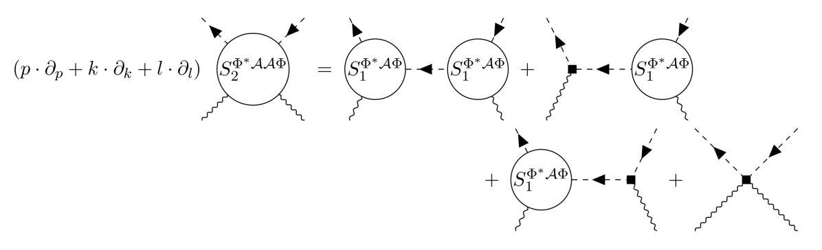
Figure 4: Diagrammatic representation of the GF-ERG equation for $(S_{2}^{\Phi^{*}\mathcal{A}\mathcal{A}\Phi})_{\mu\nu}$ given in Equation 58. The Feynman rules for the diagrams are the same as Figure 3. The conventional Wilson-Polchinski equation has the first two terms on the right-hand side, while the modification of the diffusion equation (21) entails the others.

The general solution to this equation is found to be

$$\left(S_{2}^{\Phi^{*}\Phi\mathcal{A}\mathcal{A}}(p,k,l)\right)_{\mu\nu}=c\delta_{\mu\nu}+\left(S^{\Phi^{*}\Phi\mathcal{A}}_{1}(p,k)\right)_{\mu}h_{S}(p+k)\left(S^{\Phi^{*}\Phi\mathcal{A}}_{1}(p+k,l)\right)_{\nu}\\ -\delta_{\mu\nu}\biggl{(}(p+k+l)^{2}F((p+k+l)^{2}-p^{2}-k^{2}-l^{2})+p^{2}F(p^{2}-(p+k+l)^{2}-k^{2}-l^{2})\biggr{)}-4X_{\mu\nu}(p,k,l)\,,$$ (59)

where $c$ is an arbitrary real number and $F(x)$ is defined equation 53. $X_{\mu\nu}(p,k,l)$ is a particular solution to the following equation:

$$\quantity(p\cdot\partial_{p}+k\cdot\partial_{k}+l\cdot\partial_{l})X_{\mu\nu}(p,k,l)$$

$$\qquad=(p+k+l)_{\nu}\left(S^{\Phi^{*}\Phi\mathcal{A}}_{1}(p,k)\right)_{\mu}e^{(p+k)^{2}-(p+k+l)^{2}-l^{2}}+p_{\mu}\left(S^{\Phi^{*}\Phi\mathcal{A}}_{1}(p+k,l)\right)_{\nu}e^{(p+k)^{2}-p^{2}-k^{2}}\,,$$ (60)

whose concrete form can be obtained exactly, but is very lengthy, so is given in Appendix C in Appendix C. The Ward-Takahashi identity (44) determines the arbitrary constant $c$ in Equation 59 to be $-1$, which is discussed in Appendix D. Then, $\left(S_{2}^{\Phi^{*}\Phi\mathcal{A}\mathcal{A}}(p,k,l)\right)_{\mu\nu}$ is given by

$$\left(S_{2}^{\Phi^{*}\Phi\mathcal{A}\mathcal{A}}(p,k,l)\right)_{\mu\nu}=-\delta_{\mu\nu}+\left(S^{\Phi^{*}\Phi\mathcal{A}}_{1}(p,k)\right)_{\mu}h_{S}(p+k)\left(S^{\Phi^{*}\Phi\mathcal{A}}_{1}(p+k,l)\right)_{\nu}\\ -\delta_{\mu\nu}\biggl{(}(p+k+l)^{2}F((p+k+l)^{2}-p^{2}-k^{2}-l^{2})+p^{2}F(p^{2}-(p+k+l)^{2}-k^{2}-l^{2})\biggr{)}-4X_{\mu\nu}(p,k,l)\,.$$ (61)

IV.2.2 Two-point function of gauge fields

Using the three-point vertex (54) and the four-point vertex (61), let us finally analyze the two-point correlation function of the gauge field

$$\mathcal{S}_{2}^{\mathcal{A}\mathcal{A}}=\frac{1}{2}\int_{k}\mathcal{A}_{\mu}(k)\left(e_{\tau}^{2}S_{2}^{\mathcal{A}\mathcal{A}}(k)\right)_{\mu\nu}\mathcal{A}_{\nu}(-k)\,.$$ (62)

Here, we assume $\gamma_{A}=\gamma_{1}e_{\tau}^{2}+\order{e_{\tau}^{4}}$ and then the GF-ERG equation for $\mathcal{S}_{2}^{\mathcal{A}\mathcal{A}}$ is given by

$$-(D-4)\mathcal{S}_{2}^{\mathcal{A}\mathcal{A}}-\int_{k}\quantity[\quantity(k\cdot\partial_{k}+\frac{D+2}{2})\mathcal{A}_{\mu}(k)\cdot\functionalderivative{\mathcal{S}_{2}^{\mathcal{A}\mathcal{A}}}{\mathcal{A}_{\mu}(k)}-\gamma_{1}\quantity(A_{\mu}(k)+\functionalderivative{\mathcal{S}_{0}^{(2)}}{A_{\mu}(-k)})\functionalderivative{\mathcal{S}_{0}^{(2)}}{A_{\mu}(k)}]$$

$$\quad=\int_{p}2(2p^{2}+1)\frac{\delta^{2}\mathcal{S}_{2}^{\Phi^{*}\mathcal{A}\mathcal{A}\Phi}}{\delta\phi^{*}(p)\delta\phi(p)}$$

$$\qquad+\int_{x}\Biggl{[}4i\quantity(A_{\mu}(x)+\functionalderivative{\mathcal{S}_{0}^{(2)}}{A_{\mu}(x)})\functionalderivative{\phi^{*}(x)}\partial_{\mu}\functionalderivative{\mathcal{S}_{1}^{\Phi^{*}\Phi\mathcal{A}}}{\phi(x)}+2\quantity(A_{\mu}(x)+\functionalderivative{\mathcal{S}_{0}^{(2)}}{A_{\mu}(x)})\quantity(A_{\mu}(x)+\functionalderivative{\mathcal{S}_{0}^{(2)}}{A_{\mu}(x)})\functionalderivative{\Phi(x)}{\phi(x)}+(\text{c.c.})\Biggr{]}.$$ (63)

Inserting Equation 62 into Equation 63, we obtain

$$\quantity[k\cdot\partial_{k}-2+(4-D)]\left(S_{2}^{\mathcal{A}\mathcal{A}}(k)\right)_{\mu\nu}-2\gamma_{1}k^{2}T_{\mu\nu}(k)$$

$$=\int_{p}2(2p^{2}+1)e^{-2p^{2}}h_{S}^{2}(p)\quantity(\left(S_{2}^{\Phi^{*}\Phi\mathcal{A}\mathcal{A}}(p,k,-k)\right)_{\mu\nu}+\left(S_{2}^{\Phi^{*}\Phi\mathcal{A}\mathcal{A}}(p,-k,k)\right)_{\nu\mu})$$

$$\quad-4e^{-k^{2}}\int_{p}e^{-(p+k)^{2}-p^{2}}h_{S}(p+k)h_{S}(p)\left[\left(S^{\Phi^{*}\Phi\mathcal{A}}_{1}(p,k)\right)_{\mu}(2p+k)_{\nu}+\left(S^{\Phi^{*}\Phi\mathcal{A}}_{1}(p,k)\right)_{\nu}(2p+k)_{\mu}\right]$$

$$\qquad+8e^{-2k^{2}}\delta_{\mu\nu}\int_{p}e^{-2p^{2}}h_{S}(p)\,,$$ (64)

whose diagrammatic representation is shown in Figure 5.

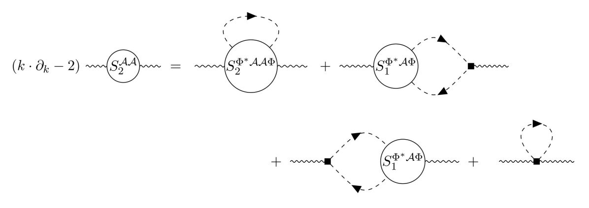
Figure 5: The diagrammatic representation of the GF-ERG equation for $\left(S_{2}^{\mathcal{A}\mathcal{A}}(k)\right)_{\mu\nu}$ in $D=4$. The Feynman rules for the diagrams are the same as Figure 3.

Here, we have symmetrized momenta and Lorentz indices on the right-hand side under $k\leftrightarrow-k$ and $\mu\leftrightarrow\nu$ because $\left(S_{2}^{\mathcal{A}\mathcal{A}}(k)\right)_{\mu\nu}$ is invariant under those replacements. We have also changed the integration variable $p\to-p$ and used the fact that $h_{S}(-q)=h_{S}(q)$, to rewrite the second term in the third line of the above equation.

Finding the solution to Equation 64 for $(S_{2}^{\mathcal{A}\mathcal{A}}(k))_{\mu\nu}$ is very complicated. Instead, we analyze here the solution in the polynomial expansion in the external momentum $k$. After tedious calculations, we find that the polynomial expansion in $k$ on the right-hand side of Equation 64 in $D=4$ is given by

$$\text{R.H.S. of \lx@cref{creftypecap~refnum}{e:eqVAsym}}=\left(S_{2}^{\mathcal{A}\mathcal{A}}(0)\right)_{\mu\nu}-\frac{2}{48\pi^{2}}k^{2}T_{\mu\nu}(k)+\order{k^{4}}\,.$$ (65)

Comparing the $O(k^{2})$ terms between the two-hand sides of Equation 64, we can read the anomalous dimension of the gauge field as

$$\gamma_{1}=\frac{1}{48\pi^{2}}\,,$$ (66)

which leads to the beta function of $e_{\tau}^{2}$ at one-loop order,

$$\partial_{\tau}e_{\tau}=-\gamma_{1}e^{3}_{\tau}=-\frac{1}{48\pi^{2}}e^{3}_{\tau}\,.$$ (67)

This result agrees with those of the ordinary perturbative computation in $D=4$. Note that due to $\partial_{\tau}=-\Lambda\partial_{\Lambda}$, the sign is opposite to the standard expression of the beta function in sQED.

Let us next investigate the loop correction to the mass term of the photon involved in equation 65 in a general spacetime dimension $D$. To this end, setting $k=0$, we find that Equation 64 is reduced to

$$\frac{2-D}{2}\left(S_{2}^{\mathcal{A}\mathcal{A}}(0)\right)_{\mu\nu} =\int_{p}2(2p^{2}+1)e^{-2p^{2}}h_{S}^{2}(p)\left(S_{2}^{\Phi^{*}\Phi\mathcal{A}\mathcal{A}}(p,0,0)\right)_{\mu\nu}$$

$$\quad-4\int_{p}e^{-2p^{2}}\quantity[h_{S}(p)\left(S^{\Phi^{*}\Phi\mathcal{A}}_{1}(p,0)\right)_{\nu}h_{S}(p)](2p_{\mu})+4\delta_{\mu\nu}\int_{p}e^{-2p^{2}}h_{S}(p)\,.$$ (68)

Using the explicit forms of $(S^{\Phi^{*}\Phi\mathcal{A}}_{1}(p,k))_{\mu}$ and $(S_{2}^{\Phi^{*}\Phi\mathcal{A}\mathcal{A}}(p,k,l))_{\mu\nu}$ given in Equation 54 and Equation 61, this equation becomes

$$\frac{2-D}{2}\left(S_{2}^{\mathcal{A}\mathcal{A}}(0)\right)_{\mu\nu}=-\frac{\Gamma\quantity(\frac{D}{2})}{(4\pi)^{D/2}}\frac{\delta_{\mu\nu}}{D}\evaluated{\quantity[\frac{4\quantity(4(p^{2})^{2}+2p^{2}+1-2e^{-2p^{2}})(p^{2})^{D/2}e^{-2p^{2}}}{(p^{2}+e^{-2p^{2}})^{2}}]}_{p=0}^{p=\infty}=0\,.$$ (69)

Thanks to the Lorentz covariance, $\left(S_{2}^{\mathcal{A}\mathcal{A}}(0)\right)_{\mu\nu}$ must be proportional to $\delta_{\mu\nu}$, and thus its coefficient gives the mass term: $\left(S_{2}^{\mathcal{A}\mathcal{A}}(0)\right)_{\mu\nu}\mathrel{\mathop{:}}=-m^{2}_{A}\delta_{\mu\nu}$. Therefore, Equation 69 means that the mass term is not generated at the 1-loop level.

This result is in contrast to the case of the conventional Wilson-Polchinski equation where the counterpart of Equation 65 reads

$$-m_{A}^{2}\delta_{\mu\nu}-\frac{2}{48\pi^{2}}k^{2}T_{\mu\nu}(k)+\order{k^{4}}\,,$$ (70)

where $m_{A}^{2}$ is expressed as the non-vanishing integral given by

$$m_{A}^{2}=\int_{p}2(2p^{2}+1)e^{-2p^{2}}h_{S}^{2}(p)(D+e^{-2p^{2}}h_{S}(p))>0.$$ (71)

This expression can be obtained by neglecting the contribution from the extra vertices, which are depicted as square dots in the Feynman diagrams and originate from the non-linear terms in the gradient flow equation in Equation 21. Comparing both cases, we see that the transversality of the photon two-point function and the anomalous dimension of the photon are consistent with perturbation theory even in the Wilson-Polchinski case, and GF-ERG holds these properties. This is because the $O(k^{2})$-term receives logarithmic corrections $\sim\log k$. The striking point is that by changing the flow equation from the simple diffusion one to the gradient flow, the quantum correction to the mass term of the photon two-point function is canceled. In this sense, the GF-ERG formulation realizes a gauge-invariant renormalization group flow in contrast to the conventional Wilson-Polchinski equation.

V Conclusions and Prospects

In this paper, we have studied scalar Quantum Electrodynamics (sQED) utilizing the Gradient Flow Exact Renormalization Group (GF-ERG) formulation. Its central idea is to focus on diffusion equations (or gradient flow equations) for fields included in the Exact Renormalization Group equation. The conventional Wilson-Polchinski equation contains simple diffusion equations like $\partial_{t}\phi^{\prime}(t,x)=\partial^{2}\phi^{\prime}(t,x)$. However, this equation is not gauge-invariant. A key point in the GF-ERG equation is to equip a gauge- (or BRST-) invariant form of diffusion equations for an Exact Renormalization Group equation.

Field ingredients in the Wilsonian effective action for sQED are the photon (U(1) gauge), Nakanishi-Lautrup, ghost, anti-ghost, and scalar matter fields. These fields obey a gauge-covariant version of the diffusion equation in GF-ERG. This approach allows us to obtain the renormalization group flow consistent with the off-shell BRST transformations for finite cutoff scales. Then, we have derived the flow equation for the Wilsonian effective action, termed the “GF-ERG equation.” In addition, we have explicitly written down the conditions for the modified BRST invariance and showed that this is reduced to the ordinary Ward-Takahashi identity under certain assumptions.

For dealing with the GF-ERG equation in sQED, we have performed perturbative calculations around the Gaussian fixed point (free theory) up to the second order of the gauge coupling $e_{\tau}$. The zeroth order action, that is, the free part was initiated from the Gaussian fixed point, and the first order correction $O(e_{\tau})$ induces a three-point photon-matter-matter vertex. For second-order contributions $O(e_{\tau}^{2})$, we have studied the photon-photon-matter-matter vertex and the photon two-point correlation function to obtain the anomalous dimension of the photon field. The result is consistent with the standard perturbation theory in four spacetime dimensions. In addition, our GF-ERG equation yields no one-loop contribution to the photon mass term. This result is unlike conventional approaches, such as the Wilson-Polchinski equation, which generally induces an artificial photon mass due to the introduction of the cutoff scale.

Our work has several implications for gauge invariance. In particular, the vertex functions (the $n$-point correlation functions) satisfy the Ward-Takahashi identity in terms of momenta at each order of the gauge coupling. This property suggests that the GF-ERG approach could provide a more robust foundation for realizing the gauge-invariant renormalization group flow. This noteworthy feature could occur not only in sQED but also in broader contexts.

As a potential avenue for future research, the consistency with the standard perturbation theory for higher vertices remains to be examined. In fact, for the matter sector, its anomalous dimension in QED has been reported to differ from the perturbation theory Miyakawa:2021wus . Thus, exploring the anomalous dimensions and beta functions of matter interactions in sQED is a significant challenge. Furthermore, extensions of GF-ERG to other gauge theories have significant potential. In the context of the asymptotic safety program, which aims to identify UV fixed points in quantum field theories with gravity, GF-ERG could be a vital computational tool for future investigations.

Acknowledgements

The authors thank Jan M. Pawlowski for intensive discussions at the initial stage of this work and for carefully reading our manuscript. J. H. acknowledges the Institute for Theoretical Physics, Heidelberg University, for the very kind hospitality during his stay. The authors also thank Hiroshi Suzuki for valuable discussions and comments. In particular, the proof of the vanishing 1-loop contribution to the photon mass is inspired by the discussion in the QED case with him. J. H. thanks the members of the Elementary Particle Theory Group at Kyushu University for their hospitality during his stay. The work of J. H. is partially supported by JSPS Grant-in-Aid for Scientific Research KAKENHI Grant No. JP21J14825. The work of M. Y. is supported by the National Science Foundation of China (NSFC) under Grant No. 12205116 and the Seeds Funding of Jilin University.

Appendix A Notation

We work on the $D$-dimensional Euclidean space. $\int_{x}$ and $\int_{p}$ are defined as

$$\int_{x}\mathrel{\mathop{:}}=\int_{\mathbb{R}^{D}}\text{d}^{D}x,\quad\int_{p}\mathrel{\mathop{:}}=\int_{\mathbb{R}^{D}}\frac{\text{d}^{D}p}{(2\pi)^{d}}\,.$$ (72)

Fourier transformation of the fields and functional derivatives are defined as

$$\phi(x) \eqqcolon\int_{p}e^{ipx}\phi(p),\qquad\functionalderivative{\phi(p)}\mathrel{\mathop{:}}=\int_{x}e^{ipx}\functionalderivative{\phi(x)}\,,$$ (73)

$$\phi^{*}(x) \eqqcolon\int_{p}e^{-ipx}\phi^{*}(p),\qquad\functionalderivative{\phi^{*}(p)}\mathrel{\mathop{:}}=\int_{x}e^{-ipx}\functionalderivative{\phi^{*}(x)}\,.$$ (74)

Appendix B Explicit form of GF-ERG equation

In this section, we discuss the explicit form of GF-ERG equation and the corresponding Wegner equation. First, we show the explicit form of the GF-ERG equation for sQED. It is given by

$$\partial_{\tau}e^{S_{\tau}}=\int_{k}\biggl{\{}\quantity(2k^{2}+\frac{D+2}{2}-\gamma_{A}+k\cdot\partial_{k})A_{\mu}(k)\cdot\functionalderivative{A_{\mu}(k)}+(2k^{2}+1-\gamma_{A})\functionalderivative{A_{\mu}(-k)}\functionalderivative{A_{\mu}(k)}\\ +\quantity(2k^{2}+\frac{D}{2}+\gamma_{A}+k\cdot\partial_{k})B(k)\cdot\functionalderivative{B(k)}-(2k^{2}+\gamma_{A})\functionalderivative{B(-k)}\functionalderivative{B(k)}\\ +\quantity(2k^{2}+\frac{D+4}{2}-\gamma_{A}+k\cdot\partial_{k})c(k)\cdot\functionalderivative{c(x)}+\quantity(2k^{2}+\frac{D}{2}+\gamma_{A}+k\cdot\partial_{k})\bar{c}(k)\cdot\functionalderivative{\bar{c}(k)}\\ +2(2k^{2}+1)\functionalderivative{\bar{c}(-k)}\functionalderivative{c(k)}\\ +\left(2k^{2}+\frac{D-2}{2}-\gamma_{\phi}+k\cdot\partial_{k}\right)\phi(k)\cdot\functionalderivative{\phi(k)}+\left(2k^{2}+\frac{D-2}{2}-\gamma_{\phi}+k\cdot\partial_{k}\right)\phi^{*}(k)\cdot\functionalderivative{\phi^{*}(k)}\\ +2\left(2k^{2}+1-2\gamma_{\phi}\right)\functionalderivative{\phi^{*}(k)}\functionalderivative{\phi(k)}\Biggr{\}}e^{S_{\tau}}\\ +\int_{x}\,\functionalderivative{\phi^{*}(x)}\Biggl{[}4ie_{\tau}\left(A_{\mu}(x)+\functionalderivative{A_{\mu}(x)}\right)\partial_{\mu}-2e_{\tau}^{2}\left(A_{\mu}(x)+\functionalderivative{A_{\mu}(x)}\right)\left(A_{\mu}(x)+\functionalderivative{A_{\mu}(x)}\right)\Biggr{]}\left(\phi^{*}(x)+\functionalderivative{\phi(x)}\right)e^{S_{\tau}}\\ +\int_{x}\,\functionalderivative{\phi(x)}\Biggl{[}-4ie_{\tau}\left(A_{\mu}(x)+\functionalderivative{A_{\mu}(x)}\right)\partial_{\mu}-2e_{\tau}^{2}\left(A_{\mu}(x)+\functionalderivative{A_{\mu}(x)}\right)\left(A_{\mu}(x)+\functionalderivative{A_{\mu}(x)}\right)\Biggr{]}\left(\phi(x)+\functionalderivative{\phi^{*}(x)}\right)e^{S_{\tau}}.$$ (75)

The last two terms on the right-hand side of this equation originate from the modification of the diffusion equation (21).

Next, let us discuss the relationship between the GF-ERG equation and the Wegner equation. For notational convention, let us denote the field contents ($A_{\mu},B,c,\bar{c}$ and $\phi$) and the corresponding gradient flow equation (21) as $\psi_{i}(x)$ and $F_{i}[\psi(x)]$, respectively. That is, the gradient flow equations are rewritten as follows:

$$\partial_{t}\psi_{i}(t,x)=F_{i}[\psi(t,x)].$$ (76)

Then, following Sonoda:2020vut , we can express the GF-ERG equation as follows:

$$\partial_{\tau}e^{S_{\tau}[\psi]}=\int_{x}\functionalderivative{\psi_{i}(x)}\hat{s}^{-1}\quantity([-d_{\psi}-\gamma_{\psi}-x\cdot\partial_{x}]\psi_{i}(x)-2F_{i}[\psi(x)])\hat{s}e^{S_{\tau}}.$$ (77)

Therefore, the coarse-graining operator $\Psi$ in the Wegner equation (27) is given by

$$\Psi=\hat{s}^{-1}\quantity([-d_{\psi}-\gamma_{\psi}-x\cdot\partial_{x}]\psi_{i}(x)-2F_{i}[\psi(x)])\hat{s}\,.$$ (78)

Indeed, the above derivation can be applied to cases with general fields, scrambler operators, and gradient flow equations, under the present definition of the Wilsonian effective action (15).

Appendix C Concrete form of $X_{\mu\nu}$

We give the concrete form of $X_{\mu\nu}$, defined by section IV.2.1. Using the formula in Appendix A in Miyakawa:2021wus , we get

$$X_{\mu\nu}(p,k,l)=\int_{0}^{1}\text{d}\alpha\,\biggl{(}(p+k+l)_{\nu}V_{\mu}(\alpha p,\alpha k)e^{\alpha^{2}(p+k)^{2}-(p+k+l)^{2}-l^{2}}+p_{\mu}V_{\nu}(\alpha(p+k),\alpha l)e^{\alpha^{2}(p+k)^{2}-p^{2}-k^{2}}\biggr{)}\,.$$ (79)

By substituting the definition (54) of $(S_{1}^{\Phi^{*}\Phi\mathcal{A}}(p,k))_{\mu}$ and executing the interal over $\alpha$, we find that $X_{\mu\nu}(p,k,l)$ is given by

$$X_{\mu\nu}(p,k,l)=(p+k+l)_{\nu}\Biggl{[}\frac{(2p+k)_{\mu}}{2}F\quantity((p+k)^{2}-(p+k+l)^{2}-l^{2})$$

$$\quad+\frac{p^{2}(p+k)_{\mu}}{p^{2}-(p+k)^{2}-k^{2}}\biggl{(}F\quantity(p^{2}-(p+k)^{2}-k^{2}+(p+k)^{2}-(p+k+l)^{2}-l^{2})-F\quantity((p+k)^{2}-(p+k+l)^{2}-l^{2})\biggr{)}$$

$$\quad+\frac{(p+k)^{2}p_{\mu}}{(p+k)^{2}-p^{2}-k^{2}}\biggl{(}F\quantity((p+k)^{2}-p^{2}-k^{2}+(p+k)^{2}-(p+k+l)^{2}-l^{2})-F\quantity((p+k)^{2}-(p+k+l)^{2}-l^{2})\biggr{)}\Biggr{]}$$

$$\quad+p_{\mu}\Biggl{[}\frac{(2p+2k+l)_{\nu}}{2}F\quantity((p+k)^{2}-p^{2}-k^{2})+\frac{(p+k)^{2}(p+k+l)_{\nu}}{(p+k)^{2}-(p+k+l)^{2}-l^{2}}$$

$$\qquad\qquad\times\biggl{(}F\quantity((p+k)^{2}-(p+k+l)^{2}-l^{2}+(p+k)^{2}-p^{2}-k^{2})-F\quantity((p+k)^{2}-p^{2}-k^{2})\biggr{)}$$

$$\quad+\frac{(p+k+l)^{2}(p+k)_{\nu}}{(p+k+l)^{2}-(p+k)^{2}-l^{2}}\biggl{(}F\quantity((p+k+l)^{2}-(p+k)^{2}-l^{2}+(p+k)^{2}-p^{2}-k^{2})-F\quantity((p+k)^{2}-p^{2}-k^{2})\biggr{)}\Biggr{]}\,.$$ (80)

Appendix D Modified BRST invariance

D.1 Reduction of modified BRST invariance

In this section, we show that the modified BRST invariance condition is reduced to the ordinary Ward-Takahashi identity under some assumption.

Before the proof, let us remind that the modified BRST invariance condition with its generator $\tilde{\hat{\mathcal{G}}}_{B}$ (42) is given by

$$0=e^{-S_{\tau}}\tilde{\hat{\mathcal{G}}}_{B}e^{S_{\tau}}=\int_{x}\biggl{[}\partial_{\mu}\quantity(c(x)+\functionalderivative{S_{\tau}}{\bar{c}(x)})\functionalderivative{S_{\tau}}{A_{\mu}(x)}+\quantity(B(x)-\functionalderivative{S_{\tau}}{B(x)})\functionalderivative{S_{\tau}}{\bar{c}(x)}\\ +\functionalderivative{A_{\mu}(x)}\partial_{\mu}\functionalderivative{S_{\tau}}{\bar{c}(x)}-\frac{\delta^{2}S_{\tau}}{\delta B(x)\delta\bar{c}(x)}+ie_{\tau}c(x)\phi(x)\functionalderivative{S_{\tau}}{\phi(x)}-ie_{\tau}c(x)\phi^{*}(x)\functionalderivative{S_{\tau}}{\phi^{*}(x)}\biggr{]}.$$ (81)

In the following, we decompose $S_{\tau}$ into the Gaussian part $S_{0}$ and the interaction part $S_{I}$ as

$$S_{\tau}=S_{0}+S_{I}$$ (82)

and show that the above equation is reduced to the ordinary Ward-Takahashi identity. We assume that $S_{I}$ is a functional only of $\mathcal{A}_{\mu},\mathcal{B},\phi$ and $\phi^{*}$;

$$S_{I}=S_{I}[\mathcal{A}_{\mu},\mathcal{B},\phi,\phi^{*}].$$ (83)

This is true for the case where the ghost sector is free, while the gauge and matter sectors have any interaction. Substituting this assumption into Equation 81 and moving onto the momentum space, we get

$$0=\int_{k}\biggl{[}ik_{\mu}e^{-k^{2}}C(k)\quantity(\functionalderivative{S_{0}}{A_{\mu}(k)}+\functionalderivative{S_{I}}{A_{\mu}(k)})+\quantity(e^{-k^{2}}\mathcal{B}(k)-\functionalderivative{S_{I}}{B(-k)})\functionalderivative{S_{0}}{\bar{c}(k)}\biggl{]}\\ +ie_{\tau}\int_{p,k}\biggl{[}e^{-k^{2}}C(k)\phi(p)\quantity(\functionalderivative{S_{0}}{\phi(p+k)}+\functionalderivative{S_{I}}{\phi(p+k)})-e^{-k^{2}}C(k)\phi^{*}(p+k)\quantity(\functionalderivative{S_{0}}{\phi(p)}+\functionalderivative{S_{I}}{\phi^{*}(p)})\biggr{]}.$$ (84)

Using the fact that the Gaussian part $S_{0}$ saturates the modified BRST invariance condition, that is, this equation also holds for the case with $S_{I}=0$, we get

$$0=\int_{k}\biggl{[}ik_{\mu}e^{-k^{2}}C(k)\functionalderivative{S_{I}}{A_{\mu}(k)}+k^{2}e^{k^{2}}C(k)\functionalderivative{S_{I}}{B(k)}+ie_{\tau}\int_{p,k}e^{-k^{2}}C(k)\quantity(\phi(p)\functionalderivative{S_{I}}{\phi(p+k)}-\phi^{*}(p+k)\functionalderivative{S_{I}}{\phi^{*}(p)})\biggr{]}.$$ (85)

Focusing on the coefficients of $e^{-k^{2}}C(k)$, we get

$$0=ik_{\mu}\functionalderivative{S_{I}}{A_{\mu}(k)}+k^{2}e^{2k^{2}}\functionalderivative{S_{I}}{B(k)}+ie_{\tau}\int_{p}\quantity(\phi(p)\functionalderivative{S_{I}}{\phi(p+k)}-\phi^{*}(p+k)\functionalderivative{S_{I}}{\phi^{*}(p)}).$$ (86)

Let us rewrite the functional derivatives $\delta/\delta A_{\mu}$ and $\delta/\delta B$ with respect to the $-1$ variables $\mathcal{A}_{\mu}$ and $\mathcal{B}$. The functional derivatives can be calculated as

$$ik_{\mu}\functionalderivative{S_{I}}{A_{\mu}(k)} =ik_{\mu}\int_{p}\quantity[\functionalderivative{\mathcal{A}_{\nu}(p)}{A_{\mu}(k)}\functionalderivative{S_{I}}{\mathcal{A}_{\nu}(p)}+\functionalderivative{\mathcal{B}(p)}{A_{\mu}(k)}\functionalderivative{S_{I}}{\mathcal{B}(p)}]$$ (87)

$$=ie^{-k^{2}}k_{\mu}h_{\mu\nu}(k)\functionalderivative{S_{I}}{\mathcal{A}_{\nu}(k)}-k^{2}e^{-k^{2}}h_{B}(k^{2})\functionalderivative{S_{I}}{\mathcal{B}(p)}$$ (88)

$$=ie^{-k^{2}}(\xi+e^{-2k^{2}})h_{B}(k^{2})k_{\mu}\functionalderivative{S_{I}}{\mathcal{A}_{\mu}(k)}-k^{2}e^{-k^{2}}h_{B}(k^{2})\functionalderivative{S_{I}}{\mathcal{B}(p)},$$ (89)

$$k^{2}e^{2k^{2}}\functionalderivative{S_{I}}{B(k)} =k^{2}e^{2k^{2}}\int_{p}\quantity[\functionalderivative{\mathcal{A}_{\mu}(p)}{B(k)}\functionalderivative{S_{I}}{\mathcal{A}_{\mu}(p)}+\functionalderivative{\mathcal{B}(p)}{B(k)}\functionalderivative{S_{I}}{\mathcal{B}(p)}]$$ (90)

$$=ik^{2}e^{k^{2}}h_{B}(k^{2})k_{\mu}\functionalderivative{S_{I}}{\mathcal{A}_{\mu}(k)}+k^{2}e^{-k^{2}}h_{B}(k^{2})\functionalderivative{S_{I}}{\mathcal{B}(k)}.$$ (91)

Summing up these terms, we obtain

$$ik_{\mu}\functionalderivative{S_{I}}{A_{\mu}(k)}+k^{2}e^{2k^{2}}\functionalderivative{S_{I}}{B(k)}=ie^{k^{2}}(k^{2}+\xi e^{-2k^{2}}+e^{-4k^{2}})h_{B}(k^{2})k_{\mu}\functionalderivative{S_{I}}{\mathcal{A}_{\mu}(k)}=ie^{k^{2}}k_{\mu}\functionalderivative{S_{I}}{\mathcal{A}_{\mu}(k)}.$$ (92)

Substituting this relation into Equation 86, we find that the modified BRST invariance condition for $S_{I}$ is given by

$$0=ie^{k^{2}}k_{\mu}\functionalderivative{S_{I}}{\mathcal{A}_{\mu}(k)}+ie_{\tau}\int_{p}\quantity(\phi(p)\functionalderivative{S_{I}}{\phi(p+k)}-\phi^{*}(p+k)\functionalderivative{S_{I}}{\phi^{*}(p)}),$$ (93)

which is nothing but the ordinary WT identity with $e^{-k^{2}}\mathcal{A}_{\mu},\phi$ and $\phi^{*}$.

D.2 Ward-Takahashi identity for vertices

In this section, we see how the Ward-Takahashi identity constrains the vertices of the Wilsonian effective action.

First order $(S_{1}^{\Phi^{*}\Phi\mathcal{A}})$

Let us see how the first order correction $S_{1}^{\Phi^{*}\Phi\mathcal{A}}$ is constrained by the Ward-Takahashi identity. Substituting $S=\mathcal{S}^{2}_{0}+e_{\tau}\mathcal{S}_{1}^{\Phi^{*}\Phi\mathcal{A}}+\order{e_{\tau}^{2}}$ into the WT identity (44) and focusing on $\Phi^{*}\Phi$-term of $\order{e_{\tau}}$, we get

$$k_{\mu}e^{k^{2}}\functionalderivative{\mathcal{S}_{1}^{\Phi^{*}\Phi\mathcal{A}}}{\mathcal{A}_{\mu}(k)}=\int_{p}\quantity(\phi^{*}(p+k)\functionalderivative{\mathcal{S}^{2}_{0}}{\phi^{*}(p)}-\phi(p)\functionalderivative{\mathcal{S}^{2}_{0}}{\phi(p+k)}),$$ (94)

which is depicted in Figure 6. Substituting the ansatz of $S_{1}^{\Phi^{*}\Phi\mathcal{A}}$ and Equation 52,

$$0 =k_{\mu}(S_{1}^{\Phi^{*}\Phi\mathcal{A}})_{\mu}(p,k)-e^{(p+k)^{2}-p^{2}-k^{2}}h_{S}^{-1}(p+k)+e^{p^{2}-(p+k)^{2}-k^{2}}h_{S}^{-1}(p)$$ (95)

$$=(a-2)p\cdot k+(b-1)k^{2}.$$ (96)

Then, we find that $(a,b)=(2,1)$ satisfies this identity for any $p$ and $k$.

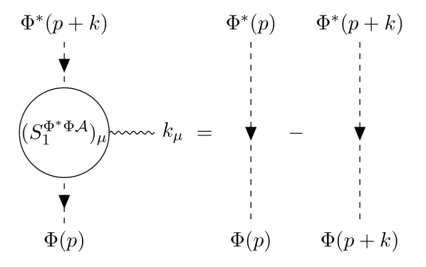
Figure 6: Diagrammatic representation of the Ward-Takahashi identity for $\mathcal{S}_{1}^{\Phi^{*}\Phi\mathcal{A}}$.

Second order $(S_{2}^{\Phi^{*}\Phi\mathcal{A}\mathcal{A}})$

Let us see how the second order correction to the four-point vertex $S_{2}^{\Phi^{*}\Phi\mathcal{A}\mathcal{A}}$ is constrained by the Ward-Takahashi identity. Substituting $S=\mathcal{S}^{2}_{0}+e_{\tau}\mathcal{S}_{1}^{\Phi^{*}\Phi\mathcal{A}}+e_{\tau}^{2}(S_{2}^{\Phi^{*}\Phi\mathcal{A}\mathcal{A}}+S_{2}^{\mathcal{A}\mathcal{A}})+\order{e_{\tau}^{3}}$ into the WT identity (44) and focusing on $\Phi^{*}\Phi\mathcal{A}$-term of $\order{e_{\tau}^{2}}$, we get

$$k_{\mu}e^{k^{2}}\functionalderivative{\mathcal{S}_{2}^{\Phi^{*}\Phi\mathcal{A}\mathcal{A}}}{\mathcal{A}_{\mu}(k)}=\int_{p}\quantity(\phi^{*}(p+k)\functionalderivative{\mathcal{S}^{\Phi^{*}\Phi\mathcal{A}}_{1}}{\phi^{*}(p)}-\phi(p)\functionalderivative{\mathcal{S}^{\Phi^{*}\Phi\mathcal{A}}_{1}}{\phi(p+k)}),$$ (97)

which is depicted in Figure 7. Substituting the concrete forms of $S_{1}^{\Phi^{*}\Phi\mathcal{A}}$ and $S_{2}^{\Phi^{*}\Phi\mathcal{A}\mathcal{A}}$, we get

$$\begin{multlined}0=k_{\mu}\quantity((S_{2}^{\Phi^{*}\Phi\mathcal{A}\mathcal{A}})_{\mu\nu}(p,k,l)+(S_{2}^{\Phi^{*}\Phi\mathcal{A}\mathcal{A}})_{\nu\mu}(p,l,k))\\ -e^{(p+k+l)^{2}-(p+l)^{2}-k^{2}}\frac{h_{S}(p+l)}{h_{S}(p+k+l)}(S_{1}^{\Phi^{*}\Phi\mathcal{A}})_{\nu}(p,l)-e^{p^{2}-(p+k)^{2}-k^{2}}\frac{h_{S}(p+k)}{h_{S}(p)}(S_{1}^{\Phi^{*}\Phi\mathcal{A}})_{\nu}(p+k,l)\end{multlined}0=k_{\mu}\quantity((S_{2}^{\Phi^{*}\Phi\mathcal{A}\mathcal{A}})_{\mu\nu}(p,k,l)+(S_{2}^{\Phi^{*}\Phi\mathcal{A}\mathcal{A}})_{\nu\mu}(p,l,k))\\ -e^{(p+k+l)^{2}-(p+l)^{2}-k^{2}}\frac{h_{S}(p+l)}{h_{S}(p+k+l)}(S_{1}^{\Phi^{*}\Phi\mathcal{A}})_{\nu}(p,l)-e^{p^{2}-(p+k)^{2}-k^{2}}\frac{h_{S}(p+k)}{h_{S}(p)}(S_{1}^{\Phi^{*}\Phi\mathcal{A}})_{\nu}(p+k,l)$$ (100)

$$\phantom{0}=2(c+1)k_{\nu}$$ (101)

Therefore, we find that the WT identity requires $c$ to be $-1$.

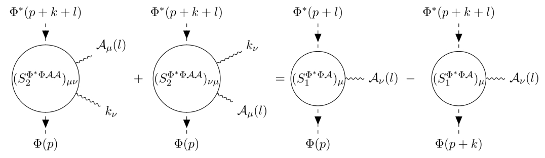
Figure 7: Diagrammatic representation of the Ward-Takahashi identity for $\mathcal{S}_{2}^{\Phi^{*}\Phi\mathcal{A}\mathcal{A}}$.

Second order $(S_{2}^{\mathcal{A}\mathcal{A}})$

Let us see how the second order correction to the four-point vertex $S_{2}^{\Phi^{*}\Phi\mathcal{A}\mathcal{A}}$ is constrained by the Ward-Takahashi identity. Substituting $S=\mathcal{S}^{2}_{0}+e_{\tau}\mathcal{S}_{1}^{\Phi^{*}\Phi\mathcal{A}}+e_{\tau}^{2}(S_{2}^{\Phi^{*}\Phi\mathcal{A}\mathcal{A}}+S_{2}^{\mathcal{A}\mathcal{A}})+\order{e_{\tau}^{3}}$ into the WT identity (44) and focusing on $\mathcal{A}$-term of $\order{e_{\tau}^{2}}$, we get

$$k_{\mu}\functionalderivative{\mathcal{S}_{2}^{\mathcal{A}\mathcal{A}}}{\mathcal{A}_{\mu}(k)}=0,$$ (102)

which is depicted in Figure 8.

Substituting the ansatz of $S_{2}^{\mathcal{A}\mathcal{A}}$, we get

$$k_{\mu}(S_{2}^{\mathcal{A}\mathcal{A}})_{\mu\nu}(k)=0,$$ (103)

which yields the transversality ($(S_{2}^{\mathcal{A}\mathcal{A}})_{\mu\nu}(k)\propto\delta_{\mu\nu}-k_{\mu}k_{\nu}/k^{2}$) of the two-point function.

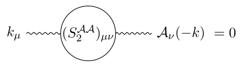
Figure 8: Diagrammatic representation of the Ward-Takahashi identity for $\mathcal{S}_{2}^{\mathcal{A}\mathcal{A}}$.

References

- (1) K. G. Wilson and J. B. Kogut, The Renormalization group and the epsilon expansion, Phys. Rept. 12 (1974) 75.
- (2) J. Polchinski, Renormalization and Effective Lagrangians, Nucl. Phys. B 231 (1984) 269.
- (3) F. J. Wegner and A. Houghton, Renormalization group equation for critical phenomena, Phys. Rev. A 8 (1973) 401.
- (4) C. Wetterich, Exact evolution equation for the effective potential, Phys. Lett. B 301 (1993) 90 [1710.05815].
- (5) T. R. Morris, The Exact renormalization group and approximate solutions, Int. J. Mod. Phys. A9 (1994) 2411 [hep-ph/9308265].
- (6) T. R. Morris, Elements of the continuous renormalization group, Prog. Theor. Phys. Suppl. 131 (1998) 395 [hep-th/9802039].
- (7) J. Berges, N. Tetradis and C. Wetterich, Nonperturbative renormalization flow in quantum field theory and statistical physics, Phys. Rept. 363 (2002) 223 [hep-ph/0005122].
- (8) K. Aoki, Introduction to the nonperturbative renormalization group and its recent applications, Int.J.Mod.Phys. B14 (2000) 1249.
- (9) C. Bagnuls and C. Bervillier, Exact renormalization group equations. An Introductory review, Phys. Rept. 348 (2001) 91 [hep-th/0002034].
- (10) J. Polonyi, Lectures on the functional renormalization group method, Central Eur. J. Phys. 1 (2003) 1 [hep-th/0110026].
- (11) J. M. Pawlowski, Aspects of the functional renormalisation group, Annals Phys. 322 (2007) 2831 [hep-th/0512261].
- (12) H. Gies, Introduction to the functional RG and applications to gauge theories, Lect. Notes Phys. 852 (2012) 287 [hep-ph/0611146].
- (13) B. Delamotte, An Introduction to the nonperturbative renormalization group, Lect. Notes Phys. 852 (2012) 49 [cond-mat/0702365].
- (14) O. J. Rosten, Fundamentals of the Exact Renormalization Group, Phys. Rept. 511 (2012) 177 [1003.1366].
- (15) P. Kopietz, L. Bartosch and F. Schütz, Introduction to the functional renormalization group, vol. 798. Springer Berlin, Heidelberg, 2010, 10.1007/978-3-642-05094-7.
- (16) J. Braun, Fermion Interactions and Universal Behavior in Strongly Interacting Theories, J. Phys. G39 (2012) 033001 [1108.4449].
- (17) N. Dupuis, L. Canet, A. Eichhorn, W. Metzner, J. M. Pawlowski, M. Tissier et al., The nonperturbative functional renormalization group and its applications, Phys. Rept. 910 (2021) 1 [2006.04853].
- (18) D. F. Litim and J. M. Pawlowski, On gauge invariance and Ward identities for the Wilsonian renormalization group, Nucl. Phys. B Proc. Suppl. 74 (1999) 325 [hep-th/9809020].
- (19) D. F. Litim and J. M. Pawlowski, On gauge invariant Wilsonian flows, in Workshop on the Exact Renormalization Group, pp. 168–185, 9, 1998, hep-th/9901063.
- (20) T. R. Morris and A. W. H. Preston, Manifestly diffeomorphism invariant classical Exact Renormalization Group, JHEP 06 (2016) 012 [1602.08993].
- (21) C. Wetterich, Gauge invariant flow equation, Nucl. Phys. B 931 (2018) 262 [1607.02989].
- (22) S. Asnafi, H. Gies and L. Zambelli, BRST invariant RG flows, Phys. Rev. D 99 (2019) 085009 [1811.03615].
- (23) Y. Igarashi, K. Itoh and T. R. Morris, BRST in the exact renormalization group, PTEP 2019 (2019) 103B01 [1904.08231].
- (24) Y. Igarashi and K. Itoh, QED in the exact renormalization group, PTEP 2021 (2021) 123B06 [2107.14012].
- (25) Y. Igarashi, K. Itoh and J. M. Pawlowski, Functional flows in QED and the modified Ward–Takahashi identity, J. Phys. A 49 (2016) 405401 [1604.08327].
- (26) G. Fejos and T. Hatsuda, Fixed point structure of the Abelian Higgs model, Phys. Rev. D 93 (2016) 121701 [1604.05849].
- (27) G. Fejos and T. Hatsuda, Renormalization group flows of the N-component Abelian Higgs model, Phys. Rev. D 96 (2017) 056018 [1705.07333].
- (28) H. Sonoda and H. Suzuki, Gradient flow exact renormalization group, PTEP 2021 (2021) 023B05 [2012.03568].
- (29) Y. Miyakawa and H. Suzuki, Gradient flow exact renormalization group: Inclusion of fermion fields, PTEP 2021 (2021) 083B04 [2106.11142].
- (30) Y. Miyakawa, H. Sonoda and H. Suzuki, Manifestly gauge invariant exact renormalization group for quantum electrodynamics, PTEP 2022 (2022) 023B02 [2111.15529].
- (31) Y. Abe, Y. Hamada and J. Haruna, Fixed point structure of the gradient flow exact renormalization group for scalar field theories, PTEP 2022 (2022) 033B03 [2201.04111].
- (32) Y. Miyakawa, H. Sonoda and H. Suzuki, Chiral anomaly as a composite operator in the gradient flow exact renormalization group formalism, PTEP 2023 (2023) 063B03 [2304.14753].
- (33) S. Dutta, B. Sathiapalan and H. Sonoda, Wilson action for the model, Nucl. Phys. B 956 (2020) 115022 [2003.02773].
- (34) F. J. Wegner, The Critical State, General Aspects, in 12th School of Modern Physics on Phase Transitions and Critical Phenomena, 1976.
- (35) J. I. Latorre and T. R. Morris, Exact scheme independence, JHEP 11 (2000) 004 [hep-th/0008123].