IPMU23-0054

Revisiting Metastable Cosmic String Breaking

Akifumi Chitose ^a, Masahiro Ibe^a,b, Yuhei Nakayama^a, Satoshi Shirai^b, and Keiichi Watanabe^a

^a ICRR, The University of Tokyo, Kashiwa, Chiba 277-8582, Japan

^b Kavli Institute for the Physics and Mathematics of the Universe (WPI),
The University of Tokyo Institutes for Advanced Study,
The University of Tokyo, Kashiwa 277-8583, Japan

1 Introduction

Topological defects arising from cosmological phase transitions have been studied intensely (see e.g., Ref. [1]). A nontrivial fundamental group of a vacuum manifold leads to linear defects called cosmic strings. In particular, a spontaneous breaking of a $\mathrm{U}$(1) symmetry leads to a string solution, since $\pi_{1}$($\mathrm{U}$(1))$=\mathbb{Z}$. Their evolution and consequences in the early Universe are indispensable topics in the new physics search, as various extensions of the Standard Model have $\mathrm{U}(1)$ symmetry.

One of the most promising potential observation channels is the gravitational waves (GWs) (for reviews see, e.g., Refs. [2, 3, 4, 5]). While topological, infinitely long strings are stable, loops and small scale structures can release energy primarily as gravitational waves. Also, repeated mutual interactions of strings lead to so-called scaling regime of the string network, in which a certain number of cosmic strings remain in the Hubble horizon. Thus, gravitational waves are continuously emitted and may be observed as the stochastic gravitational background.

International Pulsar Timing Array (IPTA) collaboration recently reported such stochastic GW signal exhibiting the Hellings–Downs angular correlation in the nHz range [6, 7]. Intriguingly, the observed spectrum favors metastable cosmic strings over stable ones as its origin [8]. The metastability of the string results in the suppression of the low-frequency spectrum of the GW in the PTA band (see also Ref. [9, 10, 11, 12, 13] for theoretical works on the GW spectrum from metastable strings). The observations by PTAs ignited tremendous research interests in metastable cosmic strings [14, 15, 16, 17, 18, 19, 13].

Metastable strings appear in models with successive symmetry breaking, e.g.,

$$G\stackrel{{\scriptstyle V}}{{\rightarrow}}\mathrm{U}(1)\stackrel{{\scriptstyle v}}{{\rightarrow}}\mbox{nothing}\ ,$$ (1.1)

with hierarchical vacuum expectation values (VEVs), $V\gg v$ [20]. Here, we presume $\pi_{1}(G)=0$ while $\pi_{2}(G/\mathrm{U}(1))=\pi_{1}(\mathrm{U}(1))=\mathbb{Z}$. In this class of models, cosmic string solutions appear as classically stable configurations in the low-energy effective theory, while they turn out to be metastable in the full theory. In fact, these models possess a monopole configuration associated with the first stage of the symmetry breaking. The strings can be cut via Schwinger production of a monopole-antimonopole pair inside, which is a tunneling process.

Conventionally, the string breaking process is approximated by a bubble formation of the monopole worldline on the string worldsheet, where the size and the thickness of the monopole and the string are taken to be zero. In particular, neglecting the monopole radius corresponds to assuming large hierarchy. In this semiclassical approximation, the resultant breaking rate per string unit length is given in Refs. [2, 20] as

$$\Gamma =\frac{\mu}{2\pi}e^{-\pi\kappa}\ ,\quad\kappa=\frac{m_{M}^{2}}{\mu}\ ,$$ (1.2)

where $\mu$ and $m_{M}$ are the string tension and the monopole mass, respectively. By using this formula, the PTA data can be well fitted for $\sqrt{\kappa}\simeq 8$ and $-7\lesssim\log_{10}G_{N}\mu\lesssim-4$ [8], where $G_{N}$ is the Newton constant.

In this paper, we revisit the estimation of the string breaking rate in light of PTAs’ GW observations. The GW spectrum in the PTA band from the metastable strings crucially depends on the breaking rate. Although the conventional approximation assumes large hierarchy between the breaking scales, it is not very significant for $\sqrt{\kappa}\sim 8$ favored by the observation. Thus, the validity of the approximation is quite unclear. To remedy this situation, we reanalyze the string breaking rate using the Ansätze on the string unwinding process proposed by Ref. [21]. An effective two dimensional field theory on the string world sheet is constructed with the soliton sizes taken into account, thereby revealing their influence on the breaking rate.

As we will see, for a large hierarchy ($\sqrt{\kappa}\gg 1$), our estimate of the bounce action $S_{B}$, which gives the tunneling factor as $e^{-S_{B}}$, agrees with the conventional one up to a factor of $O(1)$. We also obtain a robust lower limit on the tunneling factor $e^{-S_{B}}$ even for regimes the conventional estimate is unreliable.

The rest of this paper is organized as follows. In Sec. 2, we state the setup of our analysis. In Sec. 3, we introduce the unwinding Ansatz proposed in Ref. [21]. In Sec. 4, we perform numerical estimate of the bounce action. The final section is devoted to the discussions and conclusions.

2 Model with Hierarchical Breaking

2.1 Setup

For simplicity, we limit ourselves to an SU(2) gauge theory with an adjoint scalar field $\phi^{a}$ ($a=1,2,3$) and a doublet scalar field $h_{i}$ ($i=1,2$). Following Ref. [21], we take the Lagrangian as

$$\mathcal{L}=-\frac{1}{2}(D_{\mu}\phi^{a})(D^{\mu}\phi^{a})-(D_{\mu}h)^{\dagger}(D^{\mu}h)-\frac{1}{4g^{2}}F^{a}_{\mu\nu}F^{a\mu\nu}\ -V_{\mathrm{Higgs}}(\phi,h)\ ,$$ (2.1)

where $g$ is the gauge coupling constant. We take the Minkowski metric as $(g_{\mu\nu})=(-1,1,1,1)$. The covariant derivatives are given by

$$D_{\mu}h \coloneqq\partial_{\mu}h-i\frac{\tau^{a}}{2}A_{\mu}^{a}h\ ,$$ (2.2)

$$D_{\mu}\phi^{a} \coloneqq\partial_{\mu}\phi^{a}+\epsilon^{abc}A_{\mu}^{b}\phi^{c}\ ,$$ (2.3)

where $\tau$’s are the Pauli matrices and the doublet indices are suppressed. The scalar potential is given by

$$V_{\mathrm{Higgs}}(\phi,h)\coloneqq\lambda\pqty{\absolutevalue{h}^{2}-v^{2}}^{2}+\tilde{\lambda}\pqty{\phi^{a}\phi^{a}-V^{2}}^{2}+\gamma\absolutevalue{\pqty{\phi-\frac{V}{2}}h}^{2}\ ,$$ (2.4)

where $\phi\coloneqq\phi^{a}\tau^{a}/2$. The dimensionless coupling constants $\lambda$, $\tilde{\lambda}$ and $\gamma$ are taken to be positive. We also assume that the two mass scales $V$ and $v$ are hierarchical, i.e., $V\gg v$.

At the vacuum, $\phi$ takes the trivial configuration

$$\langle{\phi^{a}}\rangle=V\delta^{a3}$$ (2.5)

without loss of generality. This breaks SU(2) down to U(1). The remaining U(1) corresponds to the SO(2) rotation about the $a=3$ axis of SU(2).

Due to $\gamma>0$, the second component of $h$ obtains a large mass squared, and hence, the VEV of $h$ is given by

$$\langle h\rangle=\matrixquantity(v\\ 0)\ ,$$ (2.6)

which breaks the remaining U(1) symmetry. As the U(1) charge of $h$ is $\pm 1/2$, this breaks $\mathbb{Z}_{2}$ center symmetry of SU(2).

2.2 Monopoles

At the first phase transition SU(2)$\to$U(1), the ’t Hooft-Polyakov monopole appears as a topological defect [22, 23]. The static monopole configuration with a unit winding number at the origin is given by

$$\phi^{a}=VH(r)\displaystyle{\frac{x^{a}}{r}}\ ,\quad A_{0}^{a}=0\ ,\quad A^{a}_{i}=\displaystyle{\frac{\epsilon^{aij}x^{j}}{r^{2}}}F(r)\ ,\quad(i,j=1,2,3)\ ,$$ (2.7)

where $(x^{0},x^{1},x^{2},x^{3})$ are the spacetime coordinates and $r\coloneqq\sqrt{x_{1}^{2}+x_{2}^{2}+x_{3}^{2}}$. Assuming the hierarchy between $v$ and $V$, we neglect the effect of $h$, and set it to zero. The profile functions $H(r)$ and $F(r)$ satisfy the boundary conditions

$$H(r) \to 0,\,(r\to 0)\ , \qquad H(r) \to 1\ ,\,(r\to\infty)\ ,$$ (2.8)

$$F(r) \to 0,\,(r\to 0)\ , \qquad F(r) \to 1\ ,\,(r\to\infty)\ ,$$ (2.9)

where they approach their limits exponentially at $r\to\infty$.

To see the magnetic field, it is convenient to define the effective U(1) field strength as

$$F^{\mathrm{U}(1)}_{\mu\nu}:=\frac{1}{V}\phi^{a}F^{a}_{\mu\nu}$$ (2.10)

(see e.g., Ref. [24]). The only non-vanishing components of $F^{\mathrm{U}(1)}{}^{\mu\nu}$ are

$$F^{\mathrm{U}(1)}{}^{ij}=-\frac{\epsilon^{ijk}x^{k}}{r^{3}}(2F-F^{2})H\ ,\quad(i,j=1,2,3)\ .$$ (2.11)

Hence, the magnetic charge of the monopole is given by

$$Q^{m}:=\int_{r\to\infty}\differential S_{i}B^{\mathrm{U}(1)}{}^{i}=-4\pi\ ,$$ (2.12)

where $B^{\mathrm{U}(1)}{}^{i}=\varepsilon^{ijk}F^{\mathrm{U}(1)}_{jk}/2$ and $\differential{S}_{i}$ is the surface element of a two dimensional sphere surrounding the monopole.

The monopole mass $m_{M}$ may be parameterized as  [25, 26],

$$m_{M}=\frac{4\pi V}{g}f_{M}\quantity(\frac{m_{\phi}}{m_{W}})\ ,$$ (2.13)

where $m_{\phi}$ and $m_{W}$ are the adjoint Higgs mass and the SU(2) gauge boson mass, respectively:

$$m_{\phi}=\sqrt{8\tilde{\lambda}}V\ ,\quad m_{W}=gV\ .$$ (2.14)

Figure 1 shows $f_{M}(x)$ calculated numerically. It can be well approximated by

$$f_{M}(x)=\frac{1+16.8264x+33.7119x^{2}+12.0448x^{3}}{1+16.3264x+27.3047x^{2}+6.74157x^{3}}\ .$$ (2.15)

The limiting values are $f_{M}(x\to 0)=1$ and $f_{M}(x\to\infty)\simeq 1.787$.

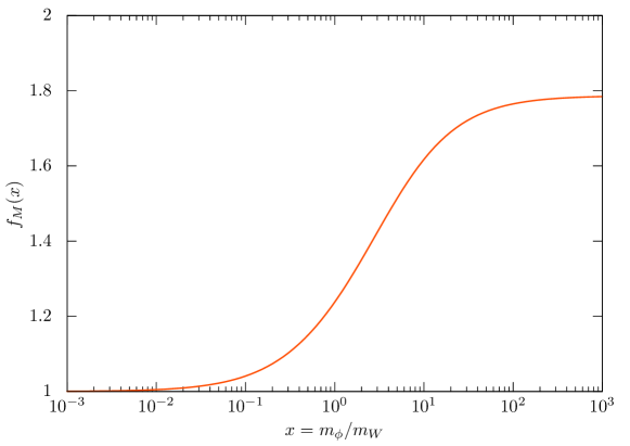
Figure 1: Monopole mass function $f_{M}(x)$ with $x=m_{\phi}/m_{W}$.

2.3 Cosmic Strings

Let us now discuss the Abrikosov-Nielsen-Olesen (ANO) string formed at the second symmetry breaking assuming the vacuum of $\phi$ in Eq. (2.5). In the large $V$ limit, $A^{1,2}$, $\phi$ and $h_{2}$ decouple from $A^{3}$ and $h_{1}$. Hence, we may treat the low-energy effective theory as a U(1) gauge theory with a complex scalar field $h_{1}$ with charge $1/2$. The covariant derivative is given by

$$D_{\mu}h_{1}=\quantity(\partial_{\mu}-\frac{i}{2}A_{\mu}^{3})h_{1}\ .$$ (2.16)

The static string solution along the $x^{3}$-axis has the form (see e.g., Ref. [1])

$$h(\rho) =\matrixquantity(h_{1}(\rho)\\ 0)\ ,$$ (2.17)

$$h_{1}(\rho) =v\xi(\rho)e^{-in\varphi}\ ,$$ (2.18)

$$A_{i}^{3} ={2n}\frac{\epsilon_{ij}x^{j}}{\rho^{2}}(1-f(\rho))\ ,~{}~{}~{}~{}(i,j=1,2)\ ,$$ (2.19)

$$A^{3}_{0} =A^{3}_{3}=0\ ,$$ (2.20)

where $n\in\mathbb{Z}$ is the winding number of the string and $\xi(\rho)$ and $f(\rho)$ are the profile functions. Here, the second component $h_{2}$ obtains a large mass, $m_{h_{2}}\coloneqq\sqrt{\gamma}V$, and thus we take $h_{2}=0$. We adopted the cylindrical coordinates $\varphi\coloneqq{\arctan}(x_{2}/x_{1})$ and $\rho\coloneqq\sqrt{x_{1}^{2}+x_{2}^{2}}$. The two-dimensional antisymmetric tensor is defined so that $\epsilon_{12}=1$. The boundary conditions for the profile functions are

$$\xi(\rho)\rightarrow 0\ ,~{}(\rho\rightarrow 0) \ ,~{}~{}~{}~{}~{}\xi(\rho)\rightarrow 1\ ,~{}(\rho\rightarrow\infty)\ ,$$ (2.21)

$$f(\rho)\rightarrow 1\ ,~{}(\rho\rightarrow 0) \ ,~{}~{}~{}~{}~{}f(\rho)\rightarrow 0\ ,~{}(\rho\rightarrow\infty)\ .$$ (2.22)

They approach unity for $\rho\gg(gv)^{-1}$ exponentially. Also, $D_{\mu}h_{1}$ approaches zero exponentially, making the string tension finite.

The winding number is related to the magnetic flux along the string by

$$\int\differential[2]{x}B_{3}=\oint_{\rho\rightarrow\infty}A_{i}^{3}\differential{x}^{i}=-{4\pi n}\ .$$ (2.23)

Thus, for $|n|=1$, the magnetic flux along a string coincides with the magnetic charge of a magnetic (anti)monopole.

The string tension may be parameterized as

$$\mu=2\pi v^{2}f_{T}\quantity(\frac{m_{h}}{m_{\gamma}})\ ,$$ (2.24)

where $m_{h}$ and $m_{\gamma}$ are the doublet Higgs mass and the massive U(1) gauge boson mass, respectively:

$$m_{h}=2\sqrt{\lambda}v\ ,\quad m_{\gamma}=\frac{1}{\sqrt{2}}gv\ .$$ (2.25)

Figure 2 shows $f_{T}(x)$ calculated numerically. It can be well approximated by

$$f_{T}(x)=\frac{\begin{aligned} \Bigl{[}0.989951&-0.266062\ln x+0.0229062(\ln x)^{2}\\ &+x\quantity(-0.0351507-0.0374918\ln x+0.0410306(\ln x)^{2})\Bigr{]}\end{aligned}}{\begin{aligned} \Bigl{[}1&-0.728749\ln x+0.195677(\ln x)^{2}\\ &-0.0229062(\ln x)^{3}+x(-0.0449826+0.0410306\ln x)\Bigr{]}\end{aligned}}\ .$$ (2.26)

Note that the tension approaches

$$\mu\to 2\pi v^{2}\ln\frac{m_{h}}{m_{\gamma}}\ ,$$ (2.27)

for $m_{h}/m_{\gamma}\gg 1$ and

$$\mu\to 2\pi v^{2}\frac{1}{\ln[m_{h}/m_{\gamma}]}\ ,$$ (2.28)

for $m_{h}/m_{\gamma}\ll 1$ (see Ref. [27]).

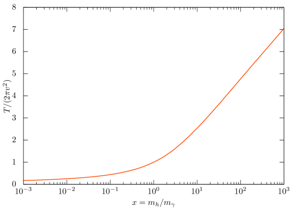
Figure 2: String tension as a function of $x=m_{h}/m_{\gamma}$.

2.4 Monopoles Connected by Cosmic String

In the full theory, the gauge symmetry is completely broken:

$$\mathop{\rm SU}(2)\stackrel{{\scriptstyle V,\,v}}{{\longrightarrow}}\mbox{nothing}\ .$$ (2.29)

Since $\pi_{2}(\mathop{\rm SU}(2))=\pi_{1}(\mathop{\rm SU}(2))=0$, no topological defects are allowed.

As we discussed above, however, we expect monopoles as well as cosmic strings at each step of the hierarchical symmetry breaking. In this subsection, we discuss how monopoles once appeared at the first symmetry breaking disappear at the next step.

To see the fate of a monopole, it is useful to adopt the gauge consisting of two slightly overlapping charts covering the northern and southern hemispheres,

$$U_{N} =\left\{(r,\theta,\varphi)|0\leq\theta\leq{\pi}/{2}+\varepsilon,\,r>R\right\}\ ,$$ (2.30)

$$U_{S} =\left\{(r,\theta,\varphi)|{\pi}/{2}-\varepsilon\leq\theta\leq\pi,\,r>R\right\}\ .$$ (2.31)

Here, $\theta$ is the zenith angle, $\varepsilon$ is a small positive number, and $R$ is some length scale satisfying $R\gg m_{W}^{-1}$. Then, the monopole configuration (2.7) transforms as

$$\phi^{a}\frac{\tau^{a}}{2} \to\phi{}_{N,S}^{a}\frac{\tau^{a}}{2}=g_{N,S}\phi^{a}\frac{\tau^{a}}{2}g_{N,S}^{\dagger}\ ,$$ (2.32)

$$A^{a}_{i}\frac{\tau^{a}}{2} \to A_{N,S\,i}^{a}\frac{\tau^{a}}{2}=g_{N,S}A_{i}^{a}\frac{\tau^{a}}{2}g_{N,S}^{\dagger}+\frac{i}{g}g_{N,S}\partial_{i}g_{N,S}^{\dagger}\ ,$$ (2.33)

with

$$g_{N}=\left(\begin{array}[]{cc}c_{\theta/2}&e^{-i\varphi}s_{\theta/2}\\ -e^{i\varphi}s_{\theta/2}&c_{\theta/2}\end{array}\right)\ ,~{}~{}~{}~{}~{}~{}~{}g_{S}=\left(\begin{array}[]{cc}e^{i\varphi}c_{\theta/2}&s_{\theta/2}\\ -s_{\theta/2}&e^{-i\varphi}c_{\theta/2}\end{array}\right)$$ (2.38)

in each chart. We call this the combed gauge.

In the combed gauge, the asymptotic behavior of the monopole at $r\gg m_{W}^{-1}$ is given by

$$\phi{}_{N}^{a} \to V\delta^{a3}\ ,\qquad A^{a}_{N}\to\delta^{a3}(\cos\theta-1)\differential{\varphi}$$ (2.39)

in the $U_{N}$ chart and

$$\phi{}^{a}_{S} \to V\delta^{a3}\ ,\qquad A^{a}_{S}\to\delta^{a3}(\cos\theta+1)\differential{\varphi}$$ (2.40)

in the $U_{S}$ chart. The other components $A^{a}_{N,S}$ ($a=1,2$) vanish asymptotically for $r\gg m_{W}^{-1}$.

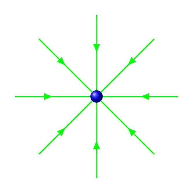
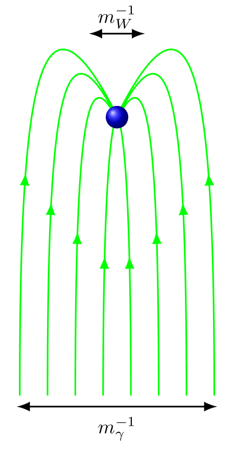
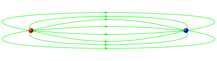
Figure 3: Schematic pictures of an isolated monopole, a monopole trapped inside a cosmic string and a monopole–antimonopole pair connected by cosmic string.

In the combed gauge, the VEV of the adjoint scalar takes the same form as the vacuum in Eq. (2.5), and hence, the U(1) gauge potential corresponds to $A_{\mu}^{3}$ far from the monopole. Due to the monopole, however, $A^{3}_{N,S}$ in each chart are connected at around the equator $\theta\sim\pi/2$ by the non-trivial gauge transition function

$$t_{NS}=e^{2i\varphi}\ ,$$ (2.41)

with which

$$A^{3}_{S}=A^{3}_{N}+2\differential{\varphi}\ .$$ (2.42)

Now we discuss the vacuum structure of $h_{1}$ around the monopole. First, let us suppose that $h_{1}$ takes a constant expectation value $v$ in the northern hemisphere in the region far from the monopole, $r\gg m_{W}^{-1}$. Then the U(1) magnetic flux of $A^{3}$ is expelled from the northern hemisphere due to the Meissner effect, and hence, the gauge potential in the northern hemisphere is trivial:

$$A^{3}_{N}=0$$ (2.43)

for $r\gg m_{W}^{-1}$. In the southern hemisphere below the overlap, on the other hand, the doublet scalar and the gauge potential take the form 

$${h_{1}}_{S} =e^{i\varphi}h_{1}{}_{N}\ ,$$ (2.44)

$$A_{S}^{3} =A_{N}^{3}+\frac{2}{g}\differential\varphi\ ,$$ (2.45)

for $r\gg m_{\gamma}^{-1}$ due to the non-trivial transition function (2.41).

As a result, the trivial configuration of $h_{1}$ in the northern hemisphere gives rise to a cosmic string configuration of $h_{1}$ with the winding number $n=-1$ in the southern hemisphere. Importantly, the magnetic charge of the monopole coincides with the magnetic flux going through the cosmic string (see Eqs. (2.12) and (2.23)). Therefore, at least one cosmic string attaches to a magnetic monopole produced at the first phase transition. The other end of the string attaches to an antimonopole (see Fig. 3). The monopole and antimonopole connected by the string eventually annihilate and disappear from the Universe.

3 String Breaking

In this section, we discuss the breaking process of cosmic strings in our model. They are spontaneously cut via a monopole-antimonopole creation inside, which is a tunneling process. In the following, we compare two kinds of estimates of the bounce action: the conventional one that neglect the soliton sizes and the one based on the Ansätze proposed in Ref. [21] which takes them into account.

3.1 Breaking of Infinitely Thin String

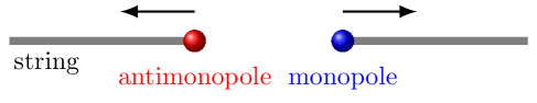
Figure 4: Cosmic string breaking through monopole-antimonopole pair production.

Here, we briefly review the conventional estimate of the string breaking rate in the infinitely thin cosmic string limit [20]. As discussed in the previous section, a cosmic string can end with a monopole in our setup. This means that a cosmic string can be cut by a monopole-antimonopole pair production as a tunneling process (see Fig. 4).

To calculate the tunneling factor, we use the Euclidean path integral method ($t=-it_{\mathrm{E}}$). In the infinitely thin string limit, the string breaking process may be regarded as a vacuum decay in 1+1 dimensions. That is, the string corresponds to the false vacuum and the absence of string corresponds to the true vacuum. The monopole plays the role of the domain wall separating the two vacua (see Fig. 5).

In the Minkowski space, the cosmic string is invariant with respect to Lorentz boosts along the string, on which we place the $z(=x^{3})$ axis. Lorentz boosts in the $(t,z)$ plane correspond to rotations in the Euclidean $(t_{\mathrm{E}},z)$ plane. We assume that the bounce solution preserves this symmetry, and hence, the domain wall separating the two vacua (i.e. monopole worldline) is a circle on the $(t_{\mathrm{E}},z)$ plane.

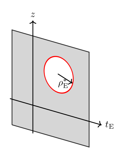
Figure 5: Bubble on the Euclidean string worldsheet. The circular monopole worldline is drawn in red.

The bounce action of the bubble is given by,

$$S_{B} =m_{M}\int_{\text{worldline}}\differential{x}-\mu\int_{\text{hole}}\differential[2]{S}$$ (3.1)

$$=2\pi{\rho_{\mathrm{E}}^{*}}m_{M}-\pi{\rho_{\mathrm{E}}^{*}}^{2}\mu\ ,$$ (3.2)

where $\mu$ is the string tension, $m_{M}$ is the monopole mass and ${\rho_{\mathrm{E}}^{*}}$ is the radius of the monopole worldline.

Maximizing this with respect to ${\rho_{\mathrm{E}}^{*}}$, we obtain

$${\rho_{\mathrm{E}}^{*}} =\frac{m_{M}}{\mu}\ ,$$ (3.3)

$$S_{B}^{(\mathrm{thin})} =\frac{\pi m_{M}^{2}}{\mu}=:\pi\kappa\ .$$ (3.4)

The string breaking rate per unit length is given by

$$\Gamma\simeq\frac{\mu}{2\pi}e^{-S_{B}^{(\mathrm{thin})}}\ .$$ (3.5)

For the the prefactor, see e.g. Ref. [33]. For reference, the recent PTA data are compatible with the GWs from metastable cosmic strings with $\sqrt{\kappa}\sim 8$.

3.2 Primitive Ansatz of Unwinding Process

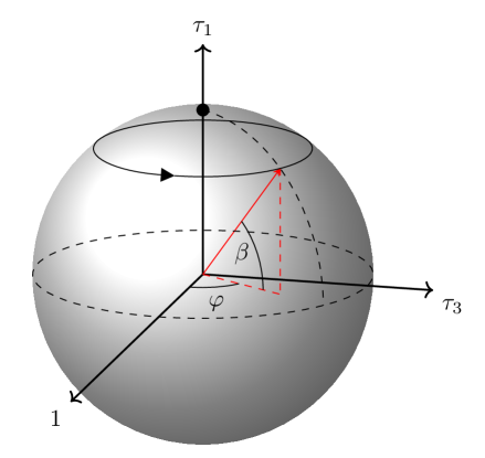
Figure 6: Unwinding of $U$ in the subspace of $\mathop{\rm SU}(2)$ without $\tau^{2}$ component. The matrix $U$ winds around the sphere at $\beta=0$, i.e., $U=e^{-i\varphi\tau^{3}}$, while $U=i\tau^{1}=\text{const.}$ at $\beta=\pi/2$.

Following Ref. [21], we parameterize the unwinding of a cosmic string with $\beta$ by introducing two Ansätze. The first one called the “primitive” Ansatz in Ref. [21] is as follows:

$$h(x) =U\pmqty{undef}\ ,$$ (3.6)

$$A_{\rho}(x) =0\ ,$$ (3.7)

$$A_{\varphi}(x) =iU(\partial_{\varphi}U^{\dagger})(1-f_{\beta}(\rho))\ ,$$ (3.8)

$$\phi(x) =VU\frac{\tau^{3}}{2}U^{\dagger}+\Delta\phi\ ,$$ (3.9)

where

$$U=e^{-i\varphi\tau^{3}}\cos\beta+i\tau^{1}\sin\beta$$ (3.10)

and

$$\Delta\phi=\Phi_{\beta}(\rho)\bqty{\frac{\tau^{1}}{2}\sin\varphi-\frac{\tau^{2}}{2}\cos\varphi}\ .$$ (3.11)

Here, we adopted the cylindrical coordinates $(t,z,\rho,\varphi)$ with the $z$ axis along the string. The boundary conditions for the profile functions are

$$\xi_{\beta}(\rho=0)=0\ ,\qquad f_{\beta}(\rho=0)=1\ ,$$ (3.12)

$$\xi_{\beta}(\rho\to\infty)=v\ ,\qquad f_{\beta}(\rho\to\infty)=0\ ,$$ (3.13)

and

$$\Phi_{\beta}(\rho=0)=V\sin 2\beta\ ,\ \qquad\Phi_{\beta}(\rho\to\infty)=0\ .$$ (3.14)

The former of Eq. 3.14 ensures $\phi$ is well-defined at $\rho=0$. For the static configuration, we take $A_{t}(x)=A_{z}(x)=0$. We will come back to this point later.

The angle $\beta$ parameterizes the winding of $h_{1}$ through the winding matrix $U\in\mathop{\rm SU}(2)$. Figure 6 shows $U$ in the $S^{2}$ subspace of SU(2) without the $\tau^{2}$ component. At $\beta=0$, $U=e^{-i\varphi\tau^{3}}$, and hence, it rotates in the $\mathbb{1}_{2}$–$\tau^{3}$ plane as $\varphi$ goes from 0 to $2\pi$. The configuration at $\beta=0$ corresponds to the cosmic string with the winding number $-1$. Intermediate $\beta$ describes a configuration with a smaller winding component (see Fig. 7). At $\beta=\pi/2$, $U=i\tau^{1}=\text{const.}$ and hence, $h_{1}$ no longer winds. In this way, the unwinding parameter $\beta$ interpolates the cosmic string $\beta=0$ and the “vacuum” $\beta=\pi/2$.

Also, Fig. 8 shows the directions of $\phi^{a}$ on the ($x_{1},x_{2}$) plane. We omitted $\Delta\phi$ which is subdominant at large $\rho$. The figure shows that $\phi^{a}$ flips as $\beta$ changes from $0$ to $\pi/2$. If one stacks Fig. 8 vertically, the arrows form the hedgehog shape, indicating the formation of a monopole.

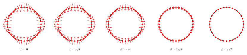
Figure 7: The winding component of $h_{1}(x)$ proportional to $e^{-i\varphi}$ projected on to the $(x_{1},x_{2})$ plane. The string is placed at the center of the circle. The direction of the winding component rotates clockwise as we circle around the cosmic string. The winding component vanishes at $\beta=\pi/2$.

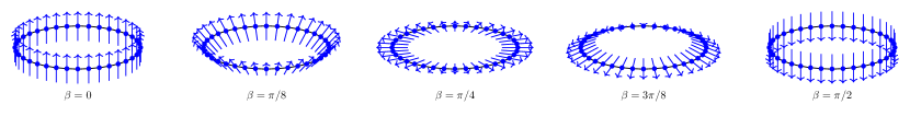
Figure 8: The directions of $\phi^{a}(x)$ on the $(x_{1},x_{2})$ plane. Here, we dropped $\Delta\phi$, which is subdominant at large $\rho$. When stacked vertically, they form the hedgehog structure.

For later use, we also display the primitive Ansatz in the singular gauge: 

$$h(x) =\pmqty{undef}\ ,$$ (3.15)

$$A_{\rho}(x) =0\ ,$$ (3.16)

$$A_{\varphi}(x) =-i(\partial_{\varphi}U^{\dagger})Uf_{\beta}(\rho)\ ,$$ (3.17)

$$\phi(x) =V\frac{\tau^{3}}{2}+U^{\dagger}(\Delta\phi)U\ .$$ (3.18)

Substituting the Ansatz into the Lagrangian (2.1) yields the string tension for a given $\beta$,

$$T(\beta)=2\pi\int_{0}^{\infty}\rho\differential{\rho}\Biggl{\{}\frac{2}{g^{2}}\frac{(\partial_{\rho}f_{\beta})^{2}}{\rho^{2}}\cos^{2}\beta+(\partial_{\rho}\xi_{\beta})^{2}+\frac{f_{\beta}^{2}}{\rho^{2}}\xi_{\beta}^{2}\cos^{2}\beta\\ +\frac{1}{2}(\partial_{\rho}\Phi_{\beta})^{2}+\frac{1}{2\rho^{2}}\bqty{\Phi_{\beta}(\cos 2\beta-2f_{\beta}\cos^{2}\beta)+Vf_{\beta}\sin 2\beta}^{2}\\ +\lambda(\xi_{\beta}^{2}-v^{2})+\tilde{\lambda}\bqty{\Phi_{\beta}^{2}-2V\Phi_{\beta}\sin 2\beta}^{2}+\frac{\gamma}{4}\Phi_{\beta}^{2}\xi_{\beta}^{2}\Biggr{\}}\ .$$ (3.19)

For a given $\beta$, the profile functions $f_{\beta}(\rho)$, $\xi_{\beta}(\rho)$ and $\Phi_{\beta}(\rho)$ are obtained by minimizing $T(\beta)$ numerically.

Figure 9 shows $T(\beta)$ for a sample parameter set, $g=1$, $m_{h}=m_{\gamma}$, $m_{W}=m_{\phi}=m_{h_{2}}=5m_{\gamma}$. The red line shows the string tension for the primitive Ansatz and the blue line shows that for the improved Ansatz introduced below. The “true” vacuum ($\beta=\pi/2$) has lower tension than the ANO string ($\beta=0$), as it should.

Incidentally, we have checked that $\beta=0$ is indeed a local minimum of the tension $T(\beta)$ for $m_{W}/m_{\gamma}\gtrsim 0.8$ for $m_{W}=m_{\phi}=m_{h_{2}}$ and $m_{h}=m_{\gamma}$. Armed with this observation, we assume that the string configuration is classically stable even for $m_{W}/m_{\gamma}=O(1)$, while the classical stability is obvious for $m_{W}/m_{\gamma}\gg 1$.

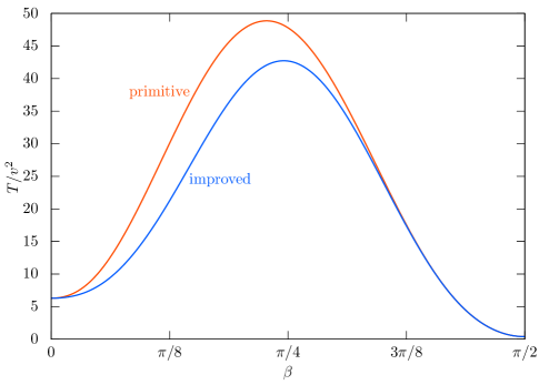
Figure 9: The string tension for a sample parameter set, $g=1$, $m_{h}=m_{\gamma}$, $m_{W}=m_{\phi}=m_{h_{2}}=5m_{\gamma}$. We show the string tension for the primitive (red) and improved (blue) Ansätze. The true vacuum $\beta=\pi/2$ has lower tension than the ANO string $\beta=0$.

3.3 Effective Description

To describe the string breaking, we promote the unwinding parameter $\beta$ to a collective coordinate for the unstable mode on the string worldsheet and construct an effective 1+1 dimensional theory of $\beta(t,z)$. In this effective theory, string breaking is described as a tunneling process of $\beta$ through the potential barrier, i.e., $T(\beta)$.

Once we introduce $(t,z)$ dependence of $\beta$, the field strength $F_{nj}$ ($n=t,z$) become singular at $\rho\to 0$ for $A_{t,z}=0$. To avoid this singularity, we need to introduce an additional profile function $a_{\beta}(\rho)$ with which, 

$$A_{n}(x)=-2(\partial_{n}\beta(t,z))\pqty{\frac{\tau^{1}}{2}\cos\varphi-\frac{\tau^{2}}{2}\sin\varphi}a_{\beta}(\rho)\ ,\quad(n=t,z)\ ,$$ (3.20)

with $a_{\beta}(0)=1$. Here, we again take the singular gauge. The finiteness of the action also requires $a_{\beta}(\infty)=0$. Note also that $A_{n}$ in Eq. 3.20 do not affect the estimate of $T(\beta)$ discussed in the previous section.

3.4 Bounce Action

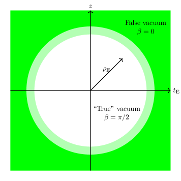
Figure 10: The bubble configuration on the Euclidean string worldsheet. The SO(2) symmetry allows the bounce solution to be parameterized by a single coordinate $\rho_{\mathrm{E}}$.

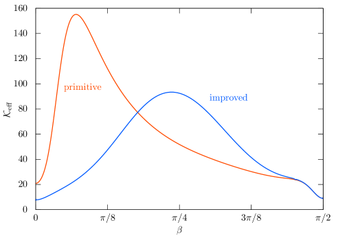
Figure 11: The coefficient $\mathcal{K}_{\mathrm{eff}}(\beta)$ of the kinetic term for the same parameter set as Fig. 9.

Once we have constructed an effective two dimensional theory of $\beta(t,z)$ on the string world sheet, the string breaking process can be regarded as a bubble formation of the “true” vacuum with $\beta\simeq\pi/2$. To calculate the bounce action of the bubble formation, we again consider the Euclidean action as in LABEL:sec:Thin_String. The Euclidean action takes the form

$$S_{\mathrm{Eucl}}=\int\differential{t}_{\mathrm{E}}\differential{z}\differential{\rho}\bqty{\frac{1}{2}(\partial_{n}\beta(t_{\mathrm{E}},z))^{2}\mathcal{H}_{\beta}(a_{\beta}(\rho),\partial_{\rho}a_{\beta}(\rho))+(\text{$a$ independent})}\ ,$$ (3.21)

where $n=(t_{\mathrm{E}},z)$. The azimuthal angle $\varphi$ of the cylindrical coordinate around the cosmic string has already been integrated out and the Jacobian is absorbed to the integrand. The prefactor of the kinetic term of $\pqty{\partial_{n}\beta}^{2}$, $\mathcal{H}_{\beta}$, is given in Appendix A.

Note that Eq. 3.21 allows us to determine $a_{\beta}(\rho)$ beforehand to find the bounce solution of $\beta(t_{\mathrm{E}},z)$. Since the bubble must minimize the action except for the direction of the bubble size, $a_{\beta}$ is determined to minimize $\int\differential{\rho}\mathcal{H}_{\beta}(a_{\beta}(\rho),\partial_{\rho}a_{\beta}(\rho))$ for each fixed $\beta$.

As discussed in Sec. 3.1, the string configuration is invariant under the Lorentz boost in $(t,z)$ plane in the Minkowski space, we assume that the bubble configuration is SO(2) invariant in $(t_{\mathrm{E}},z)$ plane. The bubble configuration for the tunneling starts from $\beta=0$ and reaches to $\beta\simeq\pi/2$ (see Fig. 10). Setting the origin of $(t_{\mathrm{E}},z)$ plane to be the bubble center and defining $\rho_{\mathrm{E}}\coloneqq\sqrt{t_{\mathrm{E}}^{2}+z^{2}}$, we have

$$S_{\mathrm{Eucl}}=2\pi\int\rho_{\mathrm{E}}\differential{\rho_{\mathrm{E}}}\int\differential{\rho}\bqty{\frac{1}{2}K(\beta(\rho_{\mathrm{E}}),\rho)(\partial_{\rho_{\mathrm{E}}}\beta(\rho_{\mathrm{E}}))^{2}+V(\beta(\rho_{\mathrm{E}}),\rho)}\ .$$ (3.22)

The explicit forms of $K$ and $V$ are given in Eq. A.2 and Eq. A.3, respectively. Carrying out the integration by $\rho$, we obtain

$$S_{\mathrm{Eucl}}=2\pi\int\rho_{\mathrm{E}}\differential{\rho_{\mathrm{E}}}\bqty{\frac{1}{2}\mathcal{K}_{\mathrm{eff}}(\beta(\rho_{\mathrm{E}}))(\partial_{\rho_{\mathrm{E}}}\beta(\rho_{\mathrm{E}}))^{2}+T(\beta(\rho_{\mathrm{E}}))}\ ,$$ (3.23)

where $\mathcal{K}_{\mathrm{eff}}(\beta)\coloneqq\int\differential{\rho}K(\beta,\rho)$ and $T(\beta)=\int\differential{\rho}V(\beta,\rho)$ is the tension in Eq. 3.19. Figure 11 shows $\mathcal{K}_{\mathrm{eff}}(\beta)$ for the same parameter set as Fig. 9.

The Euclidean equation of motion (EOM) is

$$\mathcal{K}_{\mathrm{eff}}(\beta(\rho_{\mathrm{E}}))\beta^{\prime\prime}(\rho_{\mathrm{E}})=T^{\prime}(\beta(\rho_{\mathrm{E}}))-\frac{1}{2}\mathcal{K}_{\mathrm{eff}}^{\prime}(\beta(\rho_{\mathrm{E}}))\beta^{\prime}(\rho_{\mathrm{E}})^{2}-\frac{1}{\rho_{\mathrm{E}}}\mathcal{K}_{\mathrm{eff}}(\beta(\rho_{\mathrm{E}}))\beta^{\prime}(\rho_{\mathrm{E}})\ ,$$ (3.24)

where a prime denotes the derivative with respect to the argument. By bounce solution which satisfies

$$\beta(0)\simeq\frac{\pi}{2}\ ,\ \quad\beta^{\prime}(0)=0\ ,\quad\beta(\rho_{E}\to\infty)=0\ ,$$ (3.25)

we obtain the bounce action of the unwinding process,

$$S_{B}\coloneqq\evaluated{S_{\mathrm{Eucl}}}_{\text{missing}}{bounce}-\evaluated{S_{\mathrm{Eucl}}}_{\beta=0}\ .$$ (3.26)

Thin-wall approximation

In our analysis, we solve the bounce equation numerically, where the effective $\mathcal{K}_{\mathrm{eff}}(\beta)$ and $T(\beta)$ are also estimated numerically. In the limit of $V\gg v$, however, the $T(0)-T(\pi/2)$ is much smaller than the typical height of $T(\beta)$. In such a case, the so-called thin-wall approximation provides a good estimate of the action. For later purpose, we derive the bounce action in this approximation.

The EOM (3.24) can be rewritten as

$$\derivative{\rho_{\mathrm{E}}}\bqty{\frac{1}{2}\mathcal{K}_{\mathrm{eff}}\beta^{\prime 2}-T}=\frac{1}{\rho_{\mathrm{E}}}\mathcal{K}_{\mathrm{eff}}\beta^{\prime}\ .$$ (3.27)

For $V\gg v$, the critical bubble radius ${\rho_{\mathrm{E}}^{*}}$ should be large compared to the bubble thickness. Thus, around the bubble wall, the right hand side of (3.27) effectively vanishes and the quantity in the brackets is conserved. Since the boundary condition at $\beta=0$ is $\beta^{\prime}(\rho_{\mathrm{E}})=0$,

$$\frac{1}{2}\mathcal{K}_{\mathrm{eff}}(\beta)\beta^{\prime}(\rho_{\mathrm{E}})^{2}-T(\beta)=-T(0)\ .$$ (3.28)

We evaluate the bounce action by separating it to three parts. The region outside the bubble makes no contribution as $\beta^{\prime}\approx 0$ and $T(\beta)-T(0)=0$. On the bubble wall,

$$2\pi\int_{\text{wall}}\rho_{\mathrm{E}}\differential{\rho_{\mathrm{E}}}\bqty{\frac{1}{2}\mathcal{K}_{\mathrm{eff}}(\beta)\beta^{\prime 2}+T(\beta)-T(0)} =2\pi{\rho_{\mathrm{E}}^{*}}\int_{\text{wall}}\differential{\rho_{\mathrm{E}}}\bqty{\mathcal{K}_{\mathrm{eff}}(\beta)\beta^{\prime 2}}$$ (3.29)

$$=2\pi{\rho_{\mathrm{E}}^{*}}\int_{\text{wall}}\differential{\beta}\sqrt{2\mathcal{K}_{\mathrm{eff}}(\beta)(T(\beta)-T(0))}$$ (3.30)

$$\approx 2\pi{\rho_{\mathrm{E}}^{*}}\int_{0}^{\pi/2}\differential{\beta}\sqrt{2\mathcal{K}_{\mathrm{eff}}(\beta)(T(\beta)-T(0))}$$ (3.31)

$$=:2\pi{\rho_{\mathrm{E}}^{*}}m_{\text{eff}}\ .$$ (3.32)

The contribution from the potential difference inside the wall is

$$-\pi{\rho_{\mathrm{E}}^{*}}^{2}\pqty{T(0)-T\pqty{\frac{\pi}{2}}}\ .$$ (3.33)

In total,

$$S=2\pi{\rho_{\mathrm{E}}^{*}}m_{\text{eff}}-\pi{\rho_{\mathrm{E}}^{*}}^{2}\pqty{T(0)-T\pqty{{\pi}/{2}}}\ .$$ (3.34)

Maximizing this with respect to ${\rho_{\mathrm{E}}^{*}}$, we obtain

$${\rho_{\mathrm{E}}^{*}} =\frac{m_{\text{eff}}}{T(0)-T(\pi/2)}\ ,$$ (3.35)

$$S_{B} =\evaluated{S_{\mathrm{Eucl}}}_{\text{bounce}}-\evaluated{S_{\mathrm{Eucl}}}_{\beta=0}=\frac{\pi m_{\text{eff}}^{2}}{T(0)-T(\pi/2)}\ .$$ (3.36)

Unlike ordinary vacuum decays, $S_{B}$ depends not only on the potential barrier $T(\beta)$ but also on the $\beta$-dependent mass $\mathcal{K}_{\mathrm{eff}}$.

By comparing with the bounce action in Eq. 3.4, the monopole mass $m_{M}$ is replaced by $m_{\text{eff}}$. As we will see later, they are found to be numerically close for $V\gg v$. Thus, the primitive Ansatz describes the string breaking process via the (excited) monopole-antimonopole pair creation.

3.5 Improved Ansatz

The gauge field for the primitive Ansatz in the singular gauge (3.18) may be written more explicitly as

$$A_{\varphi}=\bqty{2\cos^{2}\beta\frac{\tau^{3}}{2}-\sin 2\beta\pqty{\frac{\tau^{1}}{2}\sin\varphi+\frac{\tau^{2}}{2}\cos\varphi}}f_{\beta}(\rho)\ .$$ (3.37)

Since it depends on $\rho$ only through $f_{\beta}$, the monopole and the string must share their radial variation size. Authors of Ref. [21] argued that it leads to an overestimate of $T(\beta)$ and the bounce action, as the monopole, which has the natural size $\sim V^{-1}$, must spread over the width of the string $\sim v^{-1}$.

With this in mind, they introduced the improved Ansatz in the singular gauge:

$$A_{\varphi}=2\cos^{2}\beta\frac{\tau^{3}}{2}f^{\gamma}_{\beta}-\sin 2\beta\pqty{\frac{\tau^{1}}{2}\sin\varphi+\frac{\tau^{2}}{2}\cos\varphi}f^{W}_{\beta}\ .$$ (3.38)

We have two separate profiles for the $\tau^{3}$ component and for the others. Since the former is responsible for the string formation, $f^{\gamma}_{\beta}$ is expected to spread over $\rho\sim v^{-1}$ while $f^{W}_{\beta}$ is responsible for the monopole and should have the length scale $\sim V^{-1}$.

Requiring $A$ to be regular at $\rho=0$ in the regular gauge, we obtain the boundary conditions

$$f^{\gamma}_{\beta}(0) =f^{W}_{\beta}(0) =1\ ,$$ (3.39)

$$f^{\gamma}_{\beta}(\infty) =f^{W}_{\beta}(\infty) =0\ .$$ (3.40)

Everything else is the same as the primitive Ansatz. Corresponding $\mathcal{H}_{\beta}$, $K(\beta)$ and $V(\beta)$ are written down in Appendix A. In our numerical analysis, we compare the primitive and the improved Ansätze.

In Ref. [21], the authors argued that the primitive Ansatz overestimates the string tension by a factor of $\ln(m_{\phi}/m_{\gamma})$ for $V\gg v$ compared with the improved Ansatz. As can be seen in Fig. 9, the modification indeed reduces the string tension. However, even with large hierarchy, the improvement is not as drastic as was claimed. Contrary to their expectations, the monopole does not seem to spread to the scale $\sim v^{-1}$ even in the primitive Ansatz; rather, the string shrinks to keep the monopole small. Thus, the logarithmic enhancement is absent from both the Ansätze.

4 Numerical Results

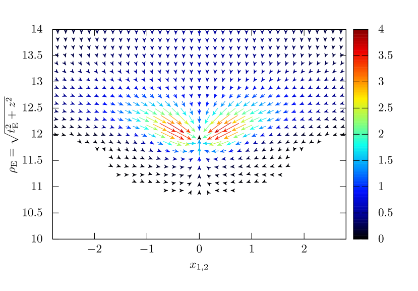
(a) Primitive Ansatz

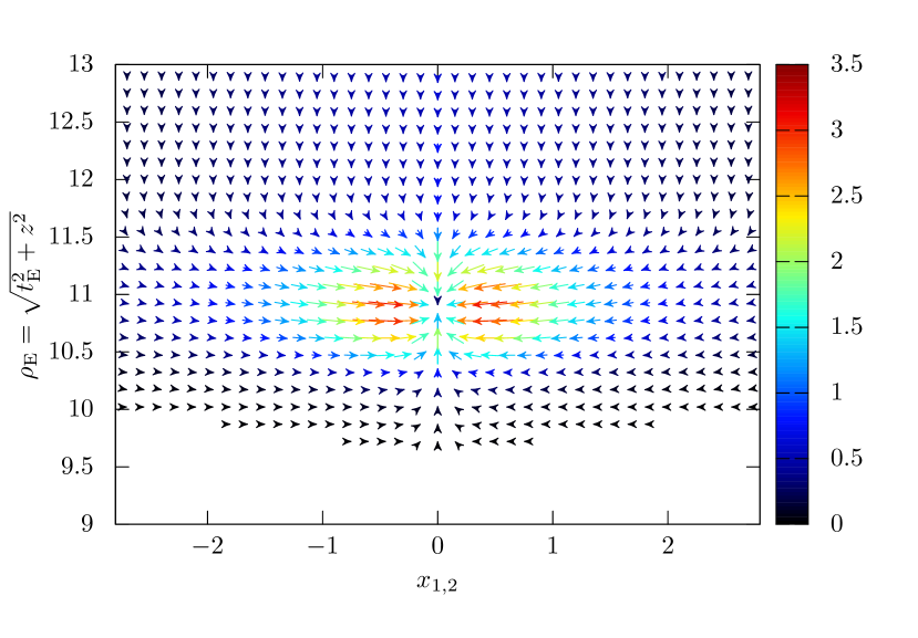
(b) Improved Ansatz

Figure 12: The magnetic field around the (excited) monopole created at the string breaking for two Ansätze. The size and color of the arrows represent the field strength. Here, we take $g=1$, $m_{h}=m_{\gamma}$, $m_{W}=m_{\phi}=m_{h_{2}}=5m_{\gamma}$ with $v=1$.

Our numerical analysis procedure is summarized below.

1. Determine profile functions $\xi_{\beta}(\rho)$, $f^{(\gamma,W)}_{\beta}(\rho)$, and $\Phi_{\beta}(\rho)$ satisfying the boundary conditions in Eqs. 3.12, 3.13 and 3.14 by minimizing $T(\beta)$ for each $\beta$.

2. Turn on the $(t,z)$ dependence of $\beta$. Substitute $\xi_{\beta}(\rho)$, $f^{(\gamma,W)}_{\beta}(\rho)$, and $\Phi_{\beta}(\rho)$ and their derivatives into $\mathcal{H}_{\beta}$ in Eq. 3.21. Determine $a_{\beta}(\rho)$ satisfying the boundary condition below Eq. 3.20 by minimizing $\int\differential{\rho}\mathcal{H}_{\beta}$.

3. Substitute the Ansatz into the action and obtain the 2D effective theory on $(t,z)$ by integrating over $(\rho,\varphi)$.

4. Obtain the bounce solution satisfying the boundary conditions (3.25) by assuming the $\operatorname{SO}(2)$ symmetry in the $(t_{\mathrm{E}},z)$ plane.

In the following, we rescale the scalar fields as $\hat{\phi}\coloneqq g\phi$ and $\hat{h}\coloneqq gh$ and parameterize the dimensionless coupling constants $\tilde{\lambda}$, ${\lambda}$ and $\gamma$ in terms of the ratios of the mass parameters:

$$\frac{\lambda}{g^{2}}=\frac{m_{h}^{2}}{8m_{\gamma}^{2}}\ ,\qquad\frac{\tilde{\lambda}}{g^{2}}=\frac{m_{\phi}^{2}}{8m_{W}^{2}}\ ,\qquad\frac{\gamma}{g^{2}}=\frac{m_{h_{2}}^{2}}{m_{W}^{2}}\ .$$ (4.1)

With this parameterization, the bounce action is proportional to $g^{-2}$, which can be factored out. Note that the same is true for the bounce action for the infinitely thin string approximation in Eq. 3.4.

Figure 12 shows the magnetic field around the (excited) monopole created at the string breaking for the two Ansätze. The magnetic monopole is at around $x_{1,2}=0$, while the cosmic string extends to the top. The magnetic flux of the cosmic string flows into the monopole. The size of the monopole (the support of $\Phi_{\beta}$) is $\sim O(m_{W}^{-1})$ and much smaller than the string width $\sim O(m_{\gamma}^{-1})$. Note that the magnetic flux disappears at $x_{1,2}\simeq 0$ since $\phi^{a}\to 0$ at $x_{1,2}\to 0$ for $\beta=\pi/4$. In the improved Ansatz, the separation of $f^{W}$ and $f^{\gamma}$ allows the magnetic field along the cosmic string to be frozen until just above the monopole (Fig. 12(b)).

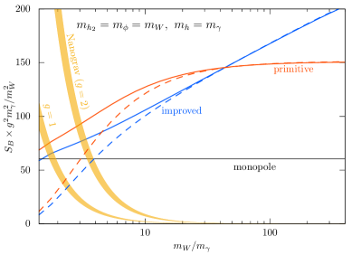
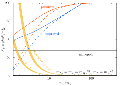
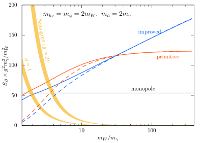
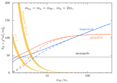
Figure 13: The bounce action normalized by $g^{2}m_{\gamma}^{2}/m_{W}^{2}$ for the primitive (red) and improved (blue) Ansätze. The dashed-lines show the thin-wall approximation of each Ansatz in (3.35). We also show the bounce action in the infinitely thin string limit $S_{B}^{\mathrm{(thin)}}$ (black). The yellow bands show the bounce action compatible with the PTA data, $S_{B}=\pi\kappa$, with $\sqrt{\kappa}=7.5$–$8.5$ for $g=1$ and $g=2$.

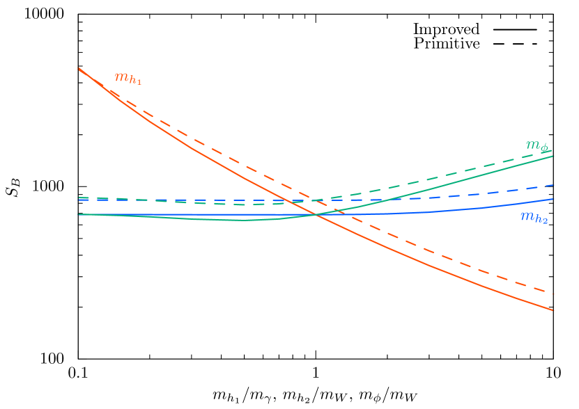
(a)

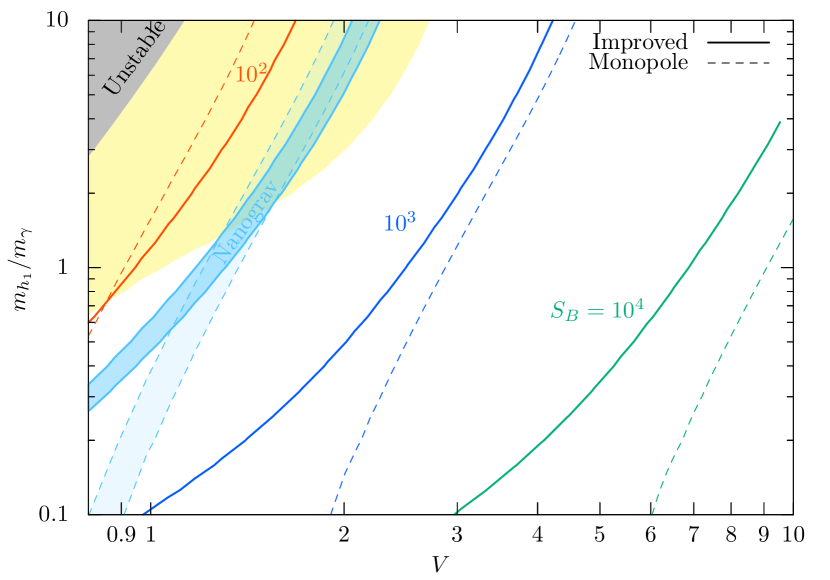
(b)

Figure 14: (a) The mass ratio dependence of $S_{B}$ with $g=1$ and $m_{W}/m_{\gamma}=5$. The solid (dashed) lines correspond to the improved (primitive) Ansatz. The bounce action is shown as a function of one of $m_{h}/m_{\gamma}$, $m_{h_{2}}/m_{W}$, $m_{\phi}/m_{W}$, with the other two fixed to unity. (b) The bounce action as a function of $V$ (with $v=1$) and $m_{h}/m_{\gamma}$, with $g=1$ and $m_{\phi}=m_{h_{2}}=m_{W}$, calculated by the improved Ansatz. The dashed lines show the bounce action by the sizeless approximation. In the yellow shaded region, the bounce action in the improved Ansatz is smaller than that in the sizeless approximation. The cyan band corresponds to the PTA data, $\sqrt{\kappa}\simeq{7.5}\text{--}{8.5}$. The lighter cyan band shows the same in the sizeless approximation.

Figure 13 shows the bounce actions normalized by $g^{2}m_{\gamma}^{2}/m_{W}^{2}$ for the primitive (red) and improved (blue) Ansätze. Bounce actions obtained by the thin-wall approximation are shown as the dashed lines. The ratios of the mass parameters are indicated in the figures. For comparison, we also show the bounce action in the infinitely thin string limit (3.4), which becomes

$$S_{B}^{(\mathrm{thin})}\times g^{2}\frac{m_{\gamma}^{2}}{m_{W}^{2}}=\frac{4\pi^{2}f_{M}^{2}(m_{\phi}/m_{W})}{f_{T}(m_{h}/m_{\gamma})}\ .$$ (4.2)

The yellow band shows the range of the bounce action compatible with the PTA data, namely $S_{B}=\pi\kappa$ with $7.5<\sqrt{\kappa}<8.5$ for $g=1$ and $g=2$.

The figures indicate that the asymptotic behavior of $S_{B}$ by the primitive Ansatz fairly reproduces that of the infinitely thin approximation, $S_{B}^{(\mathrm{thin})}$. In that region, we also found that the thin-wall approximation in Eq. 3.35 well approximates the full bounce solution, where $m_{\text{eff}}$ matches with $m_{M}$ with an accuracy of several ten percents. This is a success beyond what was expected in Ref. [21]. As a result, we confirmed that the infinitely thin limit approximation provides a fair estimate of the bounce action for $m_{W}\gg m_{\gamma}$.

The improved Ansatz, on the other hand, results in much larger bounce action for $m_{W}\gg m_{\gamma}$. The larger bounce action is due to the non-trivial kinetic function $\mathcal{K}_{\mathrm{eff}}$ which enhances the effective “potential barrier.” Thus, although the string tension for given $\beta$ is smaller for the improved Ansatz (see Fig. 9), the resultant bounce action is much larger than that of the primitive Ansatz. However, this result may be due to our procedure of minimizing $\mathcal{K}_{\mathrm{eff}}(\beta)$ and $T(\beta)$ separately as explained above, rather than a problem inherent in the Ansatz itself. Searches for a better procedure are left for a future work.

For parameter region with mild hierarchy, i.e., $m_{W}/m_{\gamma}<O(10)$, the thin-wall approximation deviates from the full bounce solution and underestimates the bounce action. The deviation is due to the rather low potential barrier compared to the difference of the “vacuum energy,” with which the thin wall approximation is no longer valid. This observation signals that the infinitely thin approximation is also not valid for the mild hierarchy since it corresponds to the thin wall approximation.

Besides, for the infinitely thin approximation, $S_{B}^{(\mathrm{thin})}$, we use the monopole mass and the string tension in the hierarchical limit, $m_{W}\gg m_{\gamma}$. For $m_{W}/m_{\gamma}=O(1)$, on the other hand, the dynamics of $\phi$ and $h$ are not well separated, and hence, the expression of $S_{B}^{(\mathrm{thin})}$ in Eq. 3.4 is no more reliable. Since the bounce action compatible with the PTA data requires $m_{W}/m_{\gamma}=O(1)$, there is a large uncertainty when interpreting bounce action in terms of monopole mass or string tension through $S_{B}^{(\mathrm{thin})}$.

The bounce actions obtained through the Ansätze, on the other hand, provide upper limits on the optimal bounce actions, since they connect the string configuration and the vacuum configurations. Thus, when interpreting the bounce action compatible with the PTA data, our results provide reliable constraints on the model parameters even for $m_{W}/m_{\gamma}=O(1)$.

Finally, we show the parameter dependence of the bounce action in Fig. 14. Figure 14(a) shows the dependence on $m_{h}/m_{\gamma}$, $m_{h_{2}}/m_{\gamma}$ and $m_{\phi}/m_{\gamma}$. The solid (dashed) lines show the dependence for the improved (primitive) Ansatz. Here, we take $g=1$ and $m_{W}/m_{\gamma}=5$. The mass parameter is taken to be $m_{\phi}=m_{W}$, $m_{h_{2}}=m_{W}$ and $m_{h}=m_{\gamma}$, respectively, when not varied. The bounce action becomes smaller for a larger $m_{h}/m_{\gamma}$, while the dependencies on $m_{h_{2}}/m_{\gamma}$ and $m_{\phi}/m_{\gamma}$ are mild.

Figure 14(b) shows the contour plot of the bounce action on $(V,m_{h}/m_{\gamma})$ plane for $g=1$ and $v=1$. The other mass parameters are set to $m_{\phi}=m_{h_{2}}=m_{W}$. The solid lines are for the improved Ansatz and the dashed lines are for the bounce action by the sizeless approximation. The gray shaded region is classically unstable for the direction of the unwinding parameter $\beta$. In the yellow shaded region, the bounce action in the improved Ansatz is smaller than $S_{B}^{(\mathrm{thin})}$, and hence, $S_{B}^{(\mathrm{thin})}$ at least underestimates the string breaking rate.

As a guidance, we also show the parameter region which results in $\sqrt{\kappa}\simeq{7.5}\text{--}{8.5}$ in the improved Ansatz as a cyan shaded region. The light-cyan shaded region corresponds to the same but with the sizeless approximation. Since the bounce action is the upper limit for given parameters, the region upper left region of the cyan shaded band cannot explain the PTA signal for $g=1$.

5 Conclusions and Discussions

In this paper, we revisited the estimate of the string breaking rate in a model with the two step symmetry breaking $\mathop{\rm SU}(2)\to\mathrm{U}(1)\to\mbox{nothing}$ with $\pi_{2}(\mathop{\rm SU}(2)/\mathrm{U}(1))=\pi_{1}(\mathrm{U}(1))=\mathbb{Z}$ while $\pi_{2}(\mathop{\rm SU}(2))=\pi_{1}(\mathop{\rm SU}(2))=0$. Based on the analytical Ansätze for the string unwinding process proposed in Ref. [21], we calculated the breaking rate which takes into account the finite sizes of the string and monopole.

As a result, we found that the asymptotic behavior of the bounce action for the primitive Ansatz well reproduces that of the bounce action in the infinitely thin approximation for $m_{W}\gg m_{\gamma}$. This is a success beyond what was expected in Ref. [21], which guarantees that the primitive Ansatz describes the breaking process via the (excited) monopole-antimonopole pair creation.

Our analysis also revealed that the thin-wall approximation results in the underestimation of the bounce action for a mild hierarchy $m_{W}/m_{\gamma}=O(10)$ or below. This deviation signals that the infinitely thin string approximation is also no more valid for $m_{W}/m_{\gamma}=O(10)$ or below.

Note that for $m_{W}/m_{\gamma}=O(1)$, which is compatible with the PTA data, the infinitely thin approximation is no longer reliable since the dynamics of $\phi$ and $h$ are not well separated. Even in such a region, the bounce action obtained in this paper can be used to provide reliable constraints on the model parameters.

Finally, we enumerate points we left for future works. Firstly, we did not show the classical stability of cosmic strings, especially for $m_{W}/m_{\gamma}=O(1)$. At least we confirmed the classical stability in the direction of the unwinding parameter $\beta$ for $m_{W}/m_{\gamma}=O(1)$. To show the classical stability, however, we need to check all the perturbations about the string configuration. We also restricted ourselves to $G=\mathop{\rm SU}(2)$ and left the extension to larger gauge groups to future work. We also did not discuss how the metastable string network is formed at the phase transition. In particular, it is highly non-trivial how many long strings are formed for $m_{W}/m_{\gamma}=O(1)$ where the phase transitions of $G\to$U(1) and U(1)$\to$nothing are not well separated. To clarify this point, we need to perform cosmological lattice simulation, which we also leave for future work.

The bounce actions we obtained in this paper provide upper limits on the bounce action of the string breaking. Thus, it is important to discuss whether there are unwinding processes which could give a smaller bounce action. For example, we find that linear combinations of the primitive and the improved Ansatz can give an $O(10)$% smaller bounce action. We will update our analysis including the improvement of the minimization of the improved Ansatz in future work.

Appendix A Long Expressions

For completeness, here we list long expressions that are too complicated and unilluminating to be included in the body.

For the primitive Ansatz,

$$\mathcal{H}_{\beta}=8\pi\rho\Biggl{[}{} \frac{1}{g^{2}}(\partial_{\rho}a_{\beta})^{2}$$

$$\begin{aligned} -a_{\beta}\biggl{\{}&-2\Phi_{\beta}(V\sin 2\beta-\Phi_{\beta})+\frac{1}{2}V(\partial_{\beta}\Phi_{\beta})\cos 2\beta\\ &+\frac{1}{g^{2}\rho^{2}}\quantity(f_{\beta}^{2}-\frac{1}{2}(\partial_{\beta}f_{\beta})\sin 2\beta-f_{\beta}(1-f_{\beta})\cos 2\beta)\biggr{\}}\end{aligned}$$

$$+a_{\beta}^{2}\Bqty{\frac{1}{g^{2}\rho^{2}}(1-4f_{\beta}(1-f_{\beta})\cos^{2}\beta)+V^{2}+\frac{1}{2}\xi_{\beta}^{2}+\Phi_{\beta}(-2V\sin 2\beta+\Phi_{\beta})}\Biggr{]}\ ,$$ (A.1)

$$K(\beta,\rho)=\mathcal{H}_{\beta}+\frac{2\pi}{g^{2}\rho}\Bigl{[}2(\partial_{\beta}f_{\beta})^{2}-4f_{\beta}\partial_{\beta}f_{\beta}\sin 2\beta+2(\partial_{\beta}f_{\beta})^{2}\cos 2\beta\\ +2g^{2}\rho^{2}(\partial_{\beta}\xi_{\beta})^{2}+g^{2}\rho^{2}(\partial_{\beta}\Phi_{\beta})^{2}+4f_{\beta}{}^{2}+4g^{2}\rho^{2}\Phi_{\beta}{}^{2}\Bigr{]}\ ,$$ (A.2)

and

$$V(\beta,\rho)=\frac{1}{2}\pi\rho\Biggl{(}\frac{8\cos^{2}\beta(\partial_{\rho}f_{\beta})^{2}}{g^{2}\rho^{2}}+4(\partial_{\rho}\xi_{\beta})^{2}+2(\partial_{\rho}\Phi_{\beta})^{2}+\frac{4\cos^{2}\beta f_{\beta}{}^{2}\xi_{\beta}{}^{2}}{\rho^{2}}\\ +\frac{8\cos^{2}\beta f_{\beta}{}^{2}\left(V\sin\beta-\cos\beta\Phi_{\beta}\right){}^{2}}{\rho^{2}}+\frac{4(\cos\beta+\cos 3\beta)f_{\beta}\Phi_{\beta}\left(V\sin\beta-\cos\beta\Phi_{\beta}\right)}{\rho^{2}}\\ +4\lambda\xi_{\beta}{}^{4}-\xi_{\beta}{}^{2}\left(8\lambda v^{2}-\gamma\Phi_{\beta}{}^{2}\right)+\frac{(\cos 4\beta+1)\Phi_{\beta}{}^{2}}{\rho^{2}}+4\tilde{\lambda}\Phi_{\beta}{}^{2}\left(\Phi_{\beta}-2V\sin 2\beta\right){}^{2}+4\lambda v^{4}\Biggr{)}\ .$$ (A.3)

For the improved ansatz,

$$\mathcal{H}_{\beta}=\frac{4\pi}{g^{2}\rho}\Bigl{[} 2\left(\partial_{\rho}a_{\beta}\right){}^{2}\rho^{2}$$

$$\begin{aligned} +a_{\beta}{}^{2}\Bigl{\{}&8f^{\gamma}_{\beta}\cos^{2}\beta\left(f^{\gamma}_{\beta}\cos^{2}\beta-1\right)+2\left((f^{W}_{\beta})^{2}\sin^{2}2\beta+g^{2}V^{2}\rho^{2}+1\right)\\ &+g^{2}\rho^{2}\left(\xi_{\beta}{}^{2}+2\Phi_{\beta}(\Phi_{\beta}-2V\sin 2\beta)\right)\Bigr{\}}\end{aligned}$$

$$\begin{aligned} +2a_{\beta}\Bigl{\{}&2f^{W}_{\beta}\left(\cos^{2}\beta\left(\left(\partial_{\beta}f^{\gamma}_{\beta}\right)\sin 2\beta-2f^{\gamma}_{\beta}\right)+\cos 2\beta\right)\\ &+\left(\partial_{\beta}f^{W}_{\beta}\right)\left(\sin 2\beta-4f^{\gamma}_{\beta}\sin\beta\cos^{3}\beta\right)\\ &-g^{2}V\left(\partial_{\beta}\Phi_{\beta}\right)\rho^{2}\cos 2\beta+2g^{2}\rho^{2}\Phi_{\beta}(V\sin 2\beta-\Phi_{\beta})\Bigr{\}}\Bigr{]}\ ,\end{aligned}$$ (A.4)

$$K(\beta,\rho)=\mathcal{H}_{\beta}+\frac{2\pi}{g^{2}\rho}\Bigl{[}4\cos^{2}\beta\quantity(\left(\partial_{\beta}f^{\gamma}_{\beta}\right)\cos\beta-2f^{\gamma}_{\beta}\sin\beta){}^{2}\\ +(2f^{W}_{\beta}\cos 2\beta+\left(\partial_{\beta}f^{W}_{\beta}\right)\sin 2\beta){}^{2}+g^{2}\rho^{2}\left(2\left(\partial_{\beta}\xi_{\beta}\right){}^{2}+\left(\partial_{\beta}\Phi_{\beta}\right){}^{2}+4\Phi_{\beta}{}^{2}\right)\Bigr{]}\ ,$$ (A.5)

and

$$V(\beta,\rho)=\frac{\pi}{2\rho}\Bigl{[}\xi_{\beta}{}^{2}\left(4\pqty{f^{\gamma}_{\beta}}^{2}\cos^{4}\beta+\pqty{f^{W}_{\beta}}^{2}\sin^{2}2\beta+\rho^{2}\left(\gamma\Phi_{\beta}{}^{2}-8\lambda v^{2}\right)\right)\\ +2f^{W}_{\beta}\Phi_{\beta}\sin 4\beta\left(2f^{\gamma}_{\beta}\cos^{2}\beta-1\right)(\Phi_{\beta}\sin 2\beta-V)\\ +\Phi_{\beta}{}^{2}\left(2f^{\gamma}_{\beta}(\cos\beta+\cos 3\beta)^{2}\left(f^{\gamma}_{\beta}\cos^{2}\beta-1\right)+\cos 4\beta\left(1-8V^{2}\rho^{2}\tilde{\lambda}\right)+8V^{2}\rho^{2}\tilde{\lambda}+1\right)\\ +2\pqty{f^{W}_{\beta}}^{2}\sin^{2}2\beta(V-\Phi_{\beta}\sin 2\beta){}^{2}\\ +\frac{1}{g^{2}}\pqty{2\left(g^{2}\rho^{2}\left(2\left(\partial_{\rho}\xi_{\beta}\right){}^{2}+\left(\partial_{\rho}\Phi_{\beta}\right){}^{2}+2\lambda v^{4}\right)+4\left(\partial_{\rho}f^{\gamma}_{\beta}\right){}^{2}\cos^{4}\beta+\left(\partial_{\rho}f^{W}_{\beta}\right){}^{2}\sin^{2}2\beta\right)}\\ +4\lambda\xi_{\beta}{}^{4}\rho^{2}-16V\rho^{2}\tilde{\lambda}\Phi_{\beta}{}^{3}\sin 2\beta+4\rho^{2}\tilde{\lambda}\Phi_{\beta}{}^{4}\Bigr{]}\ .$$ (A.6)

References

- Vilenkin and Shellard [2000] A. Vilenkin and E. P. S. Shellard, Cosmic Strings and Other Topological Defects (Cambridge University Press, 2000).
- Vilenkin [1982] A. Vilenkin, Nucl. Phys. B 196, 240 (1982).
- Hindmarsh [2011] M. Hindmarsh, Prog. Theor. Phys. Suppl. 190, 197 (2011), arXiv:1106.0391 [astro-ph.CO] .
- Auclair et al. [2020] P. Auclair et al., JCAP 04, 034 (2020), arXiv:1909.00819 [astro-ph.CO] .
- Gouttenoire et al. [2020] Y. Gouttenoire, G. Servant, and P. Simakachorn, JCAP 07, 032 (2020), arXiv:1912.02569 [hep-ph] .
- Agazie et al. [2023] G. Agazie et al. (NANOGrav), Astrophys. J. Lett. 951, L8 (2023), arXiv:2306.16213 [astro-ph.HE] .
- Antoniadis et al. [2023] J. Antoniadis et al. (EPTA, InPTA:), Astron. Astrophys. 678, A50 (2023), arXiv:2306.16214 [astro-ph.HE] .
- Afzal et al. [2023a] A. Afzal et al. (NANOGrav), Astrophys. J. Lett. 951, L11 (2023a), arXiv:2306.16219 [astro-ph.HE] .
- Leblond et al. [2009] L. Leblond, B. Shlaer, and X. Siemens, Phys. Rev. D 79, 123519 (2009), arXiv:0903.4686 [astro-ph.CO] .
- Buchmuller et al. [2020a] W. Buchmuller, V. Domcke, H. Murayama, and K. Schmitz, Phys. Lett. B 809, 135764 (2020a), arXiv:1912.03695 [hep-ph] .
- Buchmuller et al. [2020b] W. Buchmuller, V. Domcke, and K. Schmitz, Phys. Lett. B 811, 135914 (2020b), arXiv:2009.10649 [astro-ph.CO] .
- Buchmuller et al. [2021] W. Buchmuller, V. Domcke, and K. Schmitz, JCAP 12, 006 (2021), arXiv:2107.04578 [hep-ph] .
- Buchmuller et al. [2023] W. Buchmuller, V. Domcke, and K. Schmitz, JCAP 11, 020 (2023), arXiv:2307.04691 [hep-ph] .
- Lazarides et al. [2023a] G. Lazarides, R. Maji, and Q. Shafi, Phys. Rev. D 108, 095041 (2023a), arXiv:2306.17788 [hep-ph] .
- Fu et al. [2023] B. Fu, S. F. King, L. Marsili, S. Pascoli, J. Turner, and Y.-L. Zhou, (2023), arXiv:2308.05799 [hep-ph] .
- Lazarides et al. [2023b] G. Lazarides, R. Maji, A. Moursy, and Q. Shafi, (2023b), arXiv:2308.07094 [hep-ph] .
- Maji and Park [2023] R. Maji and W.-I. Park, (2023), arXiv:2308.11439 [hep-ph] .
- Afzal et al. [2023b] A. Afzal, Q. Shafi, and A. Tiwari, (2023b), arXiv:2311.05564 [hep-ph] .
- Servant and Simakachorn [2023] G. Servant and P. Simakachorn, (2023), arXiv:2312.09281 [hep-ph] .
- Preskill and Vilenkin [1993] J. Preskill and A. Vilenkin, Phys. Rev. D 47, 2324 (1993), arXiv:hep-ph/9209210 .
- Shifman and Yung [2002] M. Shifman and A. Yung, Phys. Rev. D 66, 045012 (2002), arXiv:hep-th/0205025 .
- ’t Hooft [1974] G. ’t Hooft, Nucl. Phys. B 79, 276 (1974).
- Polyakov [1974] A. M. Polyakov, JETP Lett. 20, 194 (1974).
- Shifman [2012] M. Shifman, Advanced topics in quantum field theory.: A lecture course (Cambridge Univ. Press, Cambridge, UK, 2012).
- Bogomolny and Marinov [1976] E. B. Bogomolny and M. S. Marinov, Yad. Fiz. 23, 676 (1976).
- Kirkman and Zachos [1981] T. W. Kirkman and C. K. Zachos, Phys. Rev. D 24, 999 (1981).
- Yung [1999] A. Yung, Nucl. Phys. B 562, 191 (1999), arXiv:hep-th/9906243 .
- Hindmarsh and Kibble [1985] M. Hindmarsh and T. W. B. Kibble, Phys. Rev. Lett. 55, 2398 (1985).
- Everett and Aryal [1986] A. E. Everett and M. Aryal, Phys. Rev. Lett. 57, 646 (1986).
- Kibble and Vachaspati [2015] T. W. B. Kibble and T. Vachaspati, J. Phys. G 42, 094002 (2015), arXiv:1506.02022 [astro-ph.CO] .
- Hiramatsu et al. [2021] T. Hiramatsu, M. Ibe, M. Suzuki, and S. Yamaguchi, JHEP 12, 122 (2021), arXiv:2109.12771 [hep-ph] .
- Chitose and Ibe [2023] A. Chitose and M. Ibe, Phys. Rev. D 108, 035044 (2023), arXiv:2303.10861 [hep-ph] .
- Kiselev and Selivanov [1984] V. G. Kiselev and K. G. Selivanov, JETP Lett. 39, 85 (1984).