Risk-Aware Control of Discrete-Time Stochastic Systems:
Integrating Kalman Filter and Worst-case CVaR
in Control Barrier Functions

Abstract

This paper proposes control approaches for discrete-time linear systems subject to stochastic disturbances. It employs Kalman filter to estimate the mean and covariance of the state propagation, and the worst-case conditional value-at-risk (CVaR) to quantify the tail risk using the estimated mean and covariance. The quantified risk is then integrated into a control barrier function (CBF) to derive constraints for controller synthesis, addressing tail risks near safe set boundaries. Two optimization-based control methods are presented using the obtained constraints for half-space and ellipsoidal safe sets, respectively. The effectiveness of the obtained results is demonstrated using numerical simulations.

I Introduction

Safety-critical systems such as autonomous vehicles, aerospace vehicles, and medical devices demand high reliability due to the severe consequences of their failure or malfunction, such as loss of life, significant property damage, or environmental harm. As automation becomes more prevalent in these applications, the need for risk-aware controller design is becoming increasingly essential.

In this context, Control Barrier Functions (CBFs) [1] are now recognized for their pivotal role. CBFs provide conditions for control inputs to ensure system states remain within a given safe set, thereby guaranteeing the satisfaction of safety requirements in various fields [2, 3, 4, 5].

Recent advancements in CBF approaches, such as those discussed [6, 7, 8], have incorporated external stochastic disturbances into their considerations. Moreover, some approaches consider risk through chance constraints [9], or bounds on the probability of a collision [10]. In particular, studies [11, 12, 13] provide ways of considering the safety by using the quantified tail risk to avoid severe consequences. Additionally, although many existing approaches assume that the all the system states can be observed, which may be impractical in some real applications, some [14, 15, 16, 17] deal with the cases where not all the system states can be directly accessible. Yet, comprehensive solutions addressing both stochastic disturbances and unmeasured states remain limited [14], [18].

The objective of this paper is to introduce a risk-aware control approach tailored for discrete-time linear systems affected by stochastic disturbances, where not all system states are directly observable. The approach integrates Kalman filter [19, 20] with the worst-case conditional value-at-risk (CVaR) [21, 22] and synthesizes it with a CBF framework. This integration is highly synergistic: Kalman filter provides estimates of mean and covariance of the state propagation, essential parameters for the worst-case CVaR to quantify tail risk. This combination effectively enhances controller design using CBFs.

The paper is structured as follows: Section II introduces the notation, definitions and fundamental results. Sections III - V are the main part of this paper: After introducing building blocks in Section III, sets of admissible inputs are characterized using Kalman filter along with the worst-case CVaR and the control barrier function in Section IV, which is followed by the controller design in Section V. After numerical examples in Section VI, the paper is concluded with Section VII.

II Mathematical Preliminaries

II-A Notation

The sets of real numbers, real vectors of length $n$, real matrices of size $n\times m$, real symmetric matrices of size $n$, and positive definite matrices of size $n$ are denoted by $\mathbb{R}$, $\mathbb{R}^{n}$, $\mathbb{R}^{n\times m}$, $\mathbb{S}^{n}$ and $\mathbb{S}^{n}_{+}$, respectively. For $M\in\mathbb{R}^{n\times n}$, $M\succ 0$ indicates $M$ is positive definite, $M\succcurlyeq 0$ indicates $M$ is positive semidefinite, and $\text{Tr}(M)$ denotes its the trace. For $M\in\mathbb{R}^{n\times m}$, $M^{\top}$ denotes its transpose. For a vector $v\in\mathbb{R}^{n}$, $\|v\|$ denotes its Euclidean norm, $v\geq 0$ its element-wise non-negativity, and $|v|$ the element-wise absolute value.

II-B Conditional Value-at-Risk

To present risk quantification in our approach, we begin by showing the (worst-case) CVaR.

Consider a random vector $\xi\in\mathbb{R}^{n}$ under the true distribution $\mathbb{P}$, characterized by its mean $\mu\in\mathbb{R}^{n}$ and covariance matrix $\Sigma\in\mathbb{R}^{n\times n}$. The distribution $\mathbb{P}$, representing the probability law of $\xi$, is assumed to have finite second-order moments. We define $\mathcal{P}$ as the set of all probability distributions on $\mathbb{R}^{n}$ with identical first- and second-order moments to $\mathbb{P}$. Formally,

$$\mathcal{P}=\left\{\mathbb{P}:\mathbb{E}_{\mathbb{P}}\left[\begin{bmatrix}\xi_{i}\\ 1\end{bmatrix}\begin{bmatrix}\xi_{j}\\ 1\end{bmatrix}^{\!\top}\right]=\begin{bmatrix}\Sigma\delta_{ij}&0\\ 0^{\top}&1\end{bmatrix},\forall i,j\right\},$$

where $\delta_{ij}$ is the Kronecker delta, and $\mathbb{E}_{\mathbb{P}}[\cdot]$ the expected value under $\mathbb{P}$. Although the exact form of $\mathbb{P}$ is unknown, it is clear that $\mathbb{P}\in\mathcal{P}$.

Definition II.1 (Conditional Value-at-Risk (CVaR) [23, 22])

Given a measurable loss function $L:\mathbb{R}^{n}\rightarrow\mathbb{R}$, a probability distribution $\mathbb{P}$ on $\mathbb{R}^{n}$, and a level $\varepsilon\in(0,1)$, the CVaR at level $\varepsilon$ under $\mathbb{P}$ is defined by:

$$\mathbb{P}\text{-CVaR}_{\varepsilon}[L({\xi})]=\inf_{\beta\in\mathbb{R}}\left\{\beta+\frac{1}{\varepsilon}\mathbb{E}_{\mathbb{P}}[(L({\xi})-\beta)^{+}]\right\}.$$

CVaR is the conditional expectation of losses exceeding the ($1-\varepsilon$)-quantile of $L$, quantifying the tail risk of loss function [22].

Having introduced the definition of CVaR, we now extend this concept to its worst-case scenario, key to the proposed approach. The worst-case CVaR is the supremum of CVaR over a given set of probability distributions as defined below:

Definition II.2 (Worst-case CVaR [21, 22])

The worst-case CVaR over a set of distributions $\mathcal{P}$ is:

$$\sup_{\mathbb{P}\in\mathcal{P}}\mathbb{P}\text{-CVaR}_{\varepsilon}[L({\xi})]=\inf_{\beta\in\mathbb{R}}\left\{\beta+\frac{1}{\varepsilon}\sup_{\mathbb{P}\in\mathcal{P}}\mathbb{E}_{\mathbb{P}}[(L({\xi})-\beta)^{+}]\right\}.$$

The interchangeability of the supremum and infimum is validated by the stochastic saddle point theorem [24].

The widespread adoption of (worst-case) CVaR in risk quantification is largely attributed to its coherent properties.

Proposition II.3 (Coherence properties [21, 25])

The worst-case CVaR is a coherent risk measure, i.e., it satisfies the following properties: Let $L_{1}=L_{1}(\xi)$ and $L_{2}=L_{2}(\xi)$ be two measurable loss functions, then the followings hold.

• Sub-additivity: For all $L_{1}$ and $L_{2}$,

  $$\sup_{\mathbb{P}\in\mathcal{P}}\mathbb{P}\text{-CVaR}_{\varepsilon}[L_{1}+L_{2}]$$

  $$\leq\sup_{\mathbb{P}\in\mathcal{P}}\mathbb{P}\text{-CVaR}_{\varepsilon}[L_{1}]+\sup_{\mathbb{P}\in\mathcal{P}}\mathbb{P}\text{-CVaR}_{\varepsilon}[L_{2}];$$

• Positive homogeneity: For a positive constant $c_{1}>0$,

  $$\sup_{\mathbb{P}\in\mathcal{P}}\mathbb{P}\text{-CVaR}_{\varepsilon}[c_{1}L_{1}]=c_{1}\sup_{\mathbb{P}\in\mathcal{P}}\mathbb{P}\text{-CVaR}_{\varepsilon}[L_{1}];$$

• Monotonicity: If $L_{1}\leq L_{2}$ almost surely,

  $$\sup_{\mathbb{P}\in\mathcal{P}}\mathbb{P}\text{-CVaR}_{\varepsilon}[L_{1}]\leq\sup_{\mathbb{P}\in\mathcal{P}}\mathbb{P}\text{-CVaR}_{\varepsilon}[L_{2}];$$

• Translation invariance: For a constant $c_{2}$,

  $$\sup_{\mathbb{P}\in\mathcal{P}}\mathbb{P}\text{-CVaR}_{\varepsilon}[L_{1}+c_{2}]=\sup_{\mathbb{P}\in\mathcal{P}}\mathbb{P}\text{-CVaR}_{\varepsilon}[L_{1}]+c_{2}.$$

The usefulness of the worst-case CVaR in risk quantification further appears in its computational efficiency for a special, but common, case. When the loss function $L(\xi)$ is quadratic in $\xi$, the worst-case CVaR can be computed via a semidefinite program. Let the second-order moment matrix of $\xi$

$$\Omega =\begin{bmatrix}\Sigma+\mu\mu^{\top}&\mu\\ \mu^{\top}&1\end{bmatrix}.$$

Lemma II.4 (Quadratic Loss Function [22], [26])

For $L({\xi})=\xi^{\top}P\xi+2q^{\top}\xi+r$, where $P\in\mathbb{S}^{n}$, $q\in\mathbb{R}^{n}$, and $r\in\mathbb{R}$, the worst-case CVaR is given by:

$$\sup_{\mathbb{P}\in\mathcal{P}}\mathbb{P}\text{-CVaR}_{\varepsilon}[L({\xi})]= \inf_{\beta}\left\{\beta+\frac{1}{\varepsilon}\text{Tr}(\Omega N):\right.$$

$$N\succcurlyeq 0,\ \left.N-\left[\begin{array}[]{cc}P&q\\ q^{\top}&r-\beta\end{array}\right]\succcurlyeq 0\right\}.$$

Similarly to the absolute value of a vector, we denote the element-wise worst-case CVaR by

$$\sup_{\mathbb{P}\in\mathcal{P}}\mathbb{P}\text{-CVaR}_{\varepsilon}[v]= \left[\begin{matrix}\sup_{\mathbb{P}\in\mathcal{P}}\mathbb{P}\text{-CVaR}_{\varepsilon}[e_{1}^{\top}v]\\ \vdots\\ \sup_{\mathbb{P}\in\mathcal{P}}\mathbb{P}\text{-CVaR}_{\varepsilon}[e_{n}^{\top}v]\end{matrix}\right],$$

where $e_{i}$ is the $i$th column of the identity matrix of size $n$.

Building on Lemma II.4, we now present a lemma that provides a bound on linear loss functions.

Lemma II.5 (A bound on linear $L(\xi)$[12])

Suppose $\mu=0$. Then, for $q\in\mathbb{R}^{n}$,

$$\sup_{\mathbb{P}\in\mathcal{P}}\mathbb{P}\text{-CVaR}_{\varepsilon}[q^{\top}\xi]\leq|q|^{\top}\sup_{\mathbb{P}\in\mathcal{P}}\mathbb{P}\text{-CVaR}_{\varepsilon}[\xi].$$ (1)

II-C Control Barrier Function

Having discussed the risk quantification, we now turn our attention to CBF, an approach to ensure the system safety.

Define the safe set $\mathcal{C}$ as the superlevel set of a continuously differentiable function $h:\mathbb{R}^{n}\rightarrow\mathbb{R}$,

$$\mathcal{C}=\{x\in\mathbb{R}^{n}:h(x)\geq 0\}.$$ (2)

With $\mathcal{C}$, the CBF is defined below.

Definition II.6 (Control Barrier Function (CBF) [27])

The function $h$ is a discrete-time CBF for

$$x_{t+1}=f(x_{t},u_{t})$$ (3)

on $\mathcal{C}$ if there exists an $\alpha\in[0,1)$ such that for all $x_{t}\in\mathbb{R}^{n}$, there exists a $u_{t}\in\mathbb{R}^{m}$ such that:

$$h(x_{t+1})\geq\alpha h(x_{t}).$$ (4)

The existence of a CBF guarantees that the control system is safe [28].

III Preparation: Integrating Kalman Filter and Worst-case CVaR in CBF

This is the first section of the three main sections of this paper. Here, we set up the foundational elements; system model, state estimation and CBF, for the characterization of the admissible control input and controller synthesis that follow.

III-A System Model

This paper deals with the discrete-time linear stochastic system described by:

$$\begin{aligned} x_{t+1}&=Ax_{t}+Bu_{t}+w_{t},\\ z_{t}&=Hx_{t}+v_{t},\end{aligned}$$ (5)

where $x_{t}\in\mathbb{R}^{n}$ is the state, $u_{t}\in\mathbb{R}^{m}$ is the control input, $w_{t}\in\mathbb{R}^{n_{w}}$ is the disturbance, $z_{t}\in\mathbb{R}^{n_{y}}$ is the measurement, and $v_{t}\in\mathbb{R}^{n_{v}}$ is the noise, respectively, at discrete time instant $t\in\mathbb{Z}_{\geq 0}$. The matrices $A\in\mathbb{R}^{n\times n}$, $B\in\mathbb{R}^{n\times m}$, $H\in\mathbb{R}^{n\times n_{y}}$ are assumed to be constants.

It is assumed that

• the initial state $x_{0}$ is a random vector with $\mathbb{E}[x_{0}]=\bar{x}_{0}$ and covariance $\mathbb{E}[(x_{0}-\bar{x}_{0})(x_{0}-\bar{x}_{0})^{\top}]=P_{0}$,

• the disturbance $w_{t}$ are independent and identically distributed random vectors with $\mathbb{E}[w_{t}]=0$ and finite covariance $\mathbb{E}[w_{t}w_{t}^{\top}]=Q$,

• the noise $v_{t}$ are independent and identically distributed random vectors with $\mathbb{E}[v_{t}]=0$ and finite covariance $\mathbb{E}[v_{t}v_{t}^{\top}]=R$, and

• the initial state and the noise vectors at each step $\{x_{0},w_{1},...,w_{t},v_{1},...,v_{t}\}$ are all mutually independent.

III-B Kalman Filter

We now introduce Kalman filter to estimate the mean and covariance of the state propagation.

The Kalman filter, a recursive estimator, optimal for linear systems with Gaussian noise, is adapted here for disturbances and noise, which are not necessarily Gaussians. It operates in two phases: prediction and update. In the prediction phase, the filter forecasts the next state and its uncertainty. Subsequently, during the update phase, it refines these predictions based on new measurements.

We employ standard Kalman filter notation for system (5):

• Prediction:

  • Predicted state mean at $t$: $\bar{x}_{t+1|t}=A\bar{x}_{t|t}+Bu_{t}$

  • Predicted error covariance: ${P}_{t+1|t}=AP_{t|t}A^{\top}+Q$

• Update (with gain $K_{t+1}$):

  • Measurement error covariance: $S_{t+1}=HP_{t+1|t}H^{\top}+R$ (this is used in Section V-A)

  • Updated state mean: $\bar{x}_{t+1|t+1}=\bar{x}_{t+1|t}+K_{t+1}(y_{t+1}-H\bar{x}_{t+1|t})$

  • Updated error covariance: ${P}_{t+1|t+1}=(I-K_{t+1}H)P_{t+1|t}$

How to choose the gain $K_{t+1}$ is discussed later in Section V-A.

We also let:

• $\hat{x}_{t|t}$ be the random vector with mean $\bar{x}_{t|t}$ and covariance ${P}_{t|t}$,

and

$$\hat{x}_{t+1|t}=A\hat{x}_{t|t}+Bu_{t}+w_{t}.$$ (6)

be the random vector that propagates the state $\hat{x}_{t|t}$ to the next time step according to (5). This is crucial for evaluating the condition for the control input in the next subsection.

III-C Risk-Aware CBF

This subsection integrates Kalman filter and worst-case CVaR to introduce Kalman filter-based risk-aware discrete-time CBF. This function is key for defining admissible control inputs in the subsequent section.

Consider a random vector $\xi_{t|t}$ and its shifted version $\xi_{t|t}^{c}$, defined as:

$$\xi_{t|t}=\left[\begin{matrix}\hat{x}_{t|t}^{\top}&w_{t}^{\top}\end{matrix}\right]^{\top},\ \xi_{t|t}^{c}=\xi_{t|t}-\left[\begin{matrix}\bar{x}_{t|t}^{\top}&0\end{matrix}\right]^{\top}.$$ (7)

Define

$$\mathcal{P}_{t|t}^{c}=\left\{\mathbb{P}:\mathbb{E}_{\mathbb{P}}\left[\begin{bmatrix}\xi_{i}\\ 1\end{bmatrix}\begin{bmatrix}\xi_{j}\\ 1\end{bmatrix}^{\!\top}\right]=\begin{bmatrix}\Sigma_{\xi_{t|t}^{c}}\delta_{ij}&0\\ 0^{\top}&1\end{bmatrix},\forall i,j\right\},$$ (8)

where $\Sigma_{\xi_{t|t}^{c}}=\left[\begin{array}[]{cc}{P}_{t|t}&0\\ 0&Q\end{array}\right]$. Then, the measure $\mathbb{P}$ of $\xi_{t|t}^{c}$ is $\mathbb{P}\in\mathcal{P}_{t|t}^{c}$.

With $\mathcal{C}$ in (2), we define Kalman filter-based risk-aware discrete-time CBF as below.

Definition III.1 (Control Barrier Function)

A function $h$ is a Kalman filter-based risk-aware discrete-time CBF for system (5) on $\mathcal{C}$ if there exists an $\alpha\in[0,1)$ such that for all $x_{t}\in\mathbb{R}^{n}$, there exists a $u\in\mathbb{R}^{m}$ such that:

$$\sup_{\mathbb{P}\in\mathcal{P}_{t|t}^{c}}\mathbb{P}\text{-CVaR}_{\varepsilon}[-h(\hat{x}_{t+1|t})+\alpha h(\hat{x}_{t|t})]\leq 0.$$ (9)

Here, $\hat{x}_{t|t}$ and $\hat{x}_{t+1|t}$ are computed by Kalman filter.

As we have integrated Kalman filter into CBF, Section IV will proceed to characterize sets of admissible control inputs using this, paving the way for controller synthesis.

IV Charactering the Set of Admissible Control Input Using Kalman Filter

This is the second section of the three main sections. Here, we consider characterizing the set of admissible control input by quantifying the left-hand-side of (9) to determine the control input $u_{t}$ at time $t$ in the next section. Here, we still assume that the gain $K_{t}$ is given.

IV-A Half-space safe set

We start with a half-space safe set scenario, where the set is defined by an affine function $h(x)$:

$$\begin{aligned} \mathcal{C}_{\text{hs}}&=\{x\in\mathbb{R}^{n}:h(x)=q^{\top}x+r\geq 0\}.\end{aligned}$$ (10)

This scenario allows us to reformulate the constraint (9) as a linear function of the control input $u$:

Theorem IV.1

If $h(x)=q^{\top}x+r$, $q\in\mathbb{R}^{n}$ and $r\in\mathbb{R}$, then the constraint (9) holds if and only if

$$-q^{\top}Bu_{t} \leq\phi(\hat{x}_{t|t}),$$ (11)

where

$$\begin{aligned} \phi(\hat{x}_{t|t})&=-\sup_{\mathbb{P}\in\mathcal{P}_{t|t}^{c}}\mathbb{P}\text{-CVaR}_{\varepsilon}\left[-{q}^{\top}\left[\begin{matrix}A-\alpha I&I\end{matrix}\right]\xi_{t|t}\right]\\ &\qquad+q^{\top}(A-\alpha I)\bar{x}_{t|t}+(1-\alpha)r.\end{aligned}$$ (12)

Proof:

To express the constraint in terms of the control input $u_{t}$, substitute (6) into the constraint (9):

$$\begin{aligned} &\sup_{\mathbb{P}\in\mathcal{P}_{t|t}^{c}}\mathbb{P}\text{-CVaR}_{\varepsilon}[-q^{\top}(\alpha I-A)(\hat{x}_{t|t}-\bar{x}_{t|t}+\bar{x}_{t|t}+w_{t})]\\ &\quad-q^{\top}Bu_{t}-r+\alpha r\\ =&\sup_{\mathbb{P}\in\mathcal{P}_{t|t}^{c}}\mathbb{P}\text{-CVaR}_{\varepsilon}[-q^{\top}(\alpha I-A)(\hat{x}_{t|t}-\bar{x}_{t|t}+w_{t})]\\ &\quad-q^{\top}Bu_{t}-q^{\top}(\alpha I-A)\bar{x}_{t|t}-(1-\alpha)r\leq 0.\end{aligned}$$ (13)

This is equivalent to

$$\begin{aligned} -q^{\top}Bu_{t}&\leq-\sup_{\mathbb{P}\in\mathcal{P}_{t|t}^{c}}\mathbb{P}\text{-CVaR}_{\varepsilon}\left[-{q}^{\top}\left[\begin{matrix}A-\alpha I&I\end{matrix}\right]\xi_{t|t}\right]\\ &+q^{\top}(A-\alpha I)\bar{x}_{t|t}+(1-\alpha)r=\phi(\hat{x}_{t|t}).\end{aligned}$$ (14)

∎

IV-B Ellipsoidal safe set

Next, we consider a scenario with an ellipsoidal safe set, defined by a positive definite matrix $E\in\mathbb{S}^{n}_{+}$ and a vector $x_{c}\in\mathbb{R}^{n}$:

$$\begin{aligned} \mathcal{C}_{\text{ell}}&=\{x\in\mathbb{R}^{n}:h(x)=-(x-x_{c})^{\top}E(x-x_{c})+r\geq 0\}.\end{aligned}$$ (15)

In this case, the constraint (9) can be expressed as follows:

Proposition IV.2

If $h(x)=-(x-x_{c})^{\top}E(x-x_{c})+r$, $E\in\mathbb{S}^{n}_{+}$, $x_{c}\in\mathbb{R}^{n}$ and $r\in\mathbb{R}$, then the constraint (9) is satisfied if and only if

$$\sup_{\mathbb{P}\in\mathcal{P}_{t|t}^{c}}\mathbb{P}\text{-CVaR}_{\varepsilon}\left[(\xi_{t|t}^{c})^{\top}\bar{P}\xi_{t|t}^{c}+2\bar{q}^{\top}\xi_{t|t}^{c}+\bar{r}\right]\leq 0,$$ (16)

where $\bar{P}$, $\bar{q}$, and $\bar{r}$ are defined as follows:

$$\begin{aligned} \bar{P}&=\left[\begin{matrix}A^{\top}EA-\alpha E&A^{\top}E\\ EA&E\end{matrix}\right],\\ \bar{q}&=\bar{q}_{1}+\bar{q}_{2},\\ \bar{q}_{1}&=\left[\begin{matrix}A^{\top}E(A\bar{x}_{t|t}-x_{c})-\alpha E(x-x_{c})\\ E(A\bar{x}_{t|t}-x_{c})\end{matrix}\right],\\ \bar{q}_{2}&=\left[\begin{matrix}A^{\top}EBu_{t}\\ EBu_{t}\end{matrix}\right],\\ \bar{r}&=(A\bar{x}_{t|t}+Bu_{t}-x_{c})^{\top}E(A\bar{x}_{t|t}+Bu_{t}-x_{c})\\ &-\alpha(\bar{x}_{t|t}-x_{c})^{\top}E(\bar{x}_{t|t}-x_{c})-(1-\alpha)r.\end{aligned}$$ (17)

Although checking the satisfaction of (16) for a given $u_{t}$ is straightforward, characterizing the exact set of $u_{t}$ that satisfies (16) is not except for some simple cases.

However, a sufficient condition for the constraint (9) to be satisfied can be expressed using a quadratic function of the control input $u$ as follows:

Theorem IV.3

Let $h(x)=-(x-x_{c})^{\top}E(x-x_{c})+r$ with $E\in\mathbb{S}^{n}_{+}$, $x_{c}\in\mathbb{R}^{n}$, and $r\in\mathbb{R}$. Define $\bar{u}_{t}=[u_{t}^{\top},v_{t}^{\top}]^{\top}$ as a combination of the control input $u_{t}\in\mathbb{R}^{m}$ and an auxiliary variable $v_{t}\in\mathbb{R}^{m}$. Then, the constraint (9) holds if:

$$\begin{aligned} \bar{u}_{t}^{\top}\tilde{P}\bar{u}_{t}+2\tilde{q}^{\top}(x)\bar{u}_{t}+\tilde{r}(x)\leq 0\text{ and }\ \tilde{A}\bar{u}_{t}\leq 0,\end{aligned}$$ (18)

where

$$\begin{aligned} \tilde{P}&=\left[\begin{matrix}B^{\top}EB&0\\ 0&0\end{matrix}\right],\\ \tilde{q}(x)&=\left[\begin{matrix}B^{\top}E(A\bar{x}_{t|t}-x_{c})\\ \sup_{\mathbb{P}\in\mathcal{P}_{t|t}}\mathbb{P}\text{-CVaR}_{\varepsilon}\left[\left[\begin{matrix}A^{\top}EB\\ EB\end{matrix}\right]^{\top}\xi_{t|t}^{c}\right]\end{matrix}\right],\\ \tilde{r}(x)&=\sup_{\mathbb{P}\in\mathcal{P}_{t|t}}\mathbb{P}\text{-CVaR}_{\varepsilon}\left[(\xi_{t|t}^{c})^{\top}\bar{P}\xi_{t|t}^{c}+2\bar{q}_{1}^{\top}\xi_{t|t}^{c}\right]\\ &+(A\bar{x}_{t|t}-x_{c})^{\top}E(A\bar{x}_{t|t}-x_{c})\\ &-\alpha(\bar{x}_{t|t}-x_{c})^{\top}E(\bar{x}_{t|t}-x_{c})-(1-\alpha),\\ \tilde{A}&=\left[\begin{matrix}I&-I\\ -I&-I\end{matrix}\right].\end{aligned}$$ (19)

Proof:

Applying Proposition II.3:

$$\begin{aligned} &\sup_{\mathbb{P}\in\mathcal{P}_{t|t}}\mathbb{P}\text{-CVaR}_{\varepsilon}\left[(\xi_{t|t}^{c})^{\top}\bar{P}\xi_{t|t}^{c}+2\bar{q}^{\top}\xi_{t|t}^{c}+\bar{r}\right]\\ \leq&\sup_{\mathbb{P}\in\mathcal{P}_{t|t}}\mathbb{P}\text{-CVaR}_{\varepsilon}\left[(\xi_{t|t}^{c})^{\top}\bar{P}\xi_{t|t}^{c}+2\bar{q}_{1}^{\top}\xi_{t|t}^{c}\right]\\ &\qquad+2\sup_{\mathbb{P}\in\mathcal{P}_{t|t}}\mathbb{P}\text{-CVaR}_{\varepsilon}\left[\bar{q}_{2}^{\top}\xi_{t|t}^{c}\right]+\bar{r}.\end{aligned}$$ (20)

Further, Lemma II.5 implies:

$$\begin{aligned} &\sup_{\mathbb{P}\in\mathcal{P}_{t|t}}\mathbb{P}\text{-CVaR}_{\varepsilon}\left[\bar{q}_{2}^{\top}\xi_{t|t}^{c}\right]\\ \leq&\left|u_{t}\right|^{\top}\sup_{\mathbb{P}\in\mathcal{P}_{t|t}}\mathbb{P}\text{-CVaR}_{\varepsilon}\left[\left[\begin{matrix}A^{\top}EB\\ EB\end{matrix}\right]^{\top}\xi_{t|t}^{c}\right].\end{aligned}$$ (21)

Thus, a sufficient condition for constraint satisfaction is:

$$\begin{aligned} &\sup_{\mathbb{P}\in\mathcal{P}_{t|t}}\mathbb{P}\text{-CVaR}_{\varepsilon}\left[(\xi_{t|t}^{c})^{\top}\bar{P}\xi_{t|t}^{c}+2\bar{q}_{1}^{\top}\xi_{t|t}^{c}\right]\\ &+2\left|u_{t}\right|^{\top}\sup_{\mathbb{P}\in\mathcal{P}_{t|t}}\mathbb{P}\text{-CVaR}_{\varepsilon}\left[\left[\begin{matrix}A^{\top}EB\\ EB\end{matrix}\right]^{\top}\xi_{t|t}^{c}\right]+\bar{r}\leq 0.\end{aligned}$$ (22)

Introducing $v_{t}\geq 0$ such that $-v_{t}\leq u_{t}\leq v_{t}$ and completing squares leads to the conditions in (18)-(19). ∎

V Controller Synthesis

This section, the final of the three main sections, presents the synthesis of controllers utilizing results from previous sections, and discusses the gain $K_{t+1}$ in our approach.

V-A The gain $K_{t+1}$

This subsection consider the role of the gain $K_{t+1}$ in relation to the control input $u_{t}$. Basically, the control input should satisfy the constraint (9). By looking back Lemma II.4, this left-hand-side is minimized when $\Omega$, or $\Sigma$ is small. Consequently, we employ the gain $K_{t+1}$, known as the Kalman gain, which minimizes the error covariance ${P}_{t+1|t+1}$, which corresponds to $\Sigma$. The Kalman gain is given by:

$$K_{t+1}=P_{t+1|t}H^{\top}S^{-1}_{t+1}.$$ (23)

With this, the error covariance of updated state estimate is

$${P}_{t+1|t+1}=(I-K_{t+1}H){P}_{t+1|t}.$$ (24)

Together with Section III-B, the Kalman filter formula is completed.

V-B Method 1: Modifying a nominal controller

One approach to designing a controller using (9) is to adapt a nominal controller $u_{\text{nom}}(x)$, which does not account for safety constraints, to comply with derived safety conditions by minimally modifying it so as to ensure the safety [8], [29]. The control input at $t$ can be computed by

$$\begin{aligned} u^{*}(x)&=\text{argmin}_{u}\|u-u_{\text{nom}}(x)\|^{2}\\ \text{s.t. }\ &\text{CBF constraint \eqref{eq:or_cbf} e.g., \eqref{eq:hs}, \eqref{eq:ell-const}}.\end{aligned}$$ (25)

This method prioritizes safety while minimizing deviation from the nominal controller. If infeasible, a modified optimization problem incorporating a penalty parameter $\rho>0$ to balance safety and controller deviation can be used. In case of the ellipsoidal safe set, for example, the constraint (18) is revised:

$$\begin{aligned} u^{*}(x)&=\text{argmin}_{u}\|u-u_{\text{nom}}(x)\|^{2}+\rho\delta\\ \text{s.t. }\ &\bar{u}_{t}^{\top}\tilde{P}\bar{u}_{t}+2\tilde{q}^{\top}(x)\bar{u}_{t}+\tilde{r}(x)\leq\delta\text{ and }\tilde{A}\bar{u}_{t}\leq 0.\end{aligned}$$ (26)

V-C Method 2: CLF-CBF-based optimization

Another approach is to combine Control Lyapunov Functions (CLF) and CBF to obtain the control inputs [30, 28].

Let us first define the CLF:

Definition V.1 (Control Lyapunov Function [2])

A map $V:\mathbb{R}^{n}\rightarrow\mathbb{R}$ is an exponential control Lyapunov function for the system $x_{t+1}=f(x_{t},u_{t})$ if there exists:

• positive constants $c_{1}$ and $c_{2}$ such that $c_{1}\|x_{t}\|^{2}\leq V(x_{t})\leq c_{2}\|x_{t}\|^{2}$, and

• a control input $u_{t}:\mathbb{R}^{m}\rightarrow\mathbb{R}$, $\forall x_{t}\in\mathbb{R}^{n}$ and $c_{3}>0$ such that $V(x_{t+1})-V(x_{t})+c_{3}\|x_{t}\|^{2}\leq 0$.

We consider aiming at stabilizing the estimated mean states $\bar{x}_{t|t}$, $\bar{x}_{t+1|t}$ by choosing an appropriate $V$ and forcing the condition $V(\bar{x}_{t+1|t})-V(\bar{x}_{t|t})+c_{3}\|\bar{x}_{t|t}\|^{2}\leq 0$.

Choose

$$V(x_{t})=x_{t}^{\top}\Phi x_{t}$$ (27)

for some $\Phi\in\mathbb{S}^{n}_{+}$. Choosing $c_{1}=\sigma_{\min}$ and $c_{2}=\sigma_{\max}$, where $\sigma_{\min}$ and $\sigma_{\max}$ are the smallest and largest singular values of $\Phi$, respectively, satisfies the first condition of CLF.

For the second condition to be satisfied, $u_{t}$ must exist such that satisfies the quadratic constraint.

$$\begin{aligned} &V(\bar{x}_{t+1|t})-V(\bar{x}_{t|t})+c_{3}\|\bar{x}_{t|t}\|^{2}\\ =&(A\bar{x}_{t|t}+Bu_{t})^{\top}\Phi(A\bar{x}_{t|t}+Bu_{t})-\bar{x}_{t|t}^{\top}\Phi\bar{x}_{t|t}+c_{3}\|\bar{x}_{t|t}\|^{2}\\ =&u_{t}^{\top}B^{\top}\Phi Bu_{t}+2(A\bar{x}_{t|t})^{\top}\Phi Bu_{t}\\ &\qquad+\bar{x}_{t|t}^{\top}(A^{\top}\Phi A-\Phi+c_{3}I)\bar{x}_{t|t}\leq 0.\end{aligned}$$ (28)

Combining this with the CBF constraint, at each time, the control input can be computed by

$$\begin{aligned} \mathbf{v}^{*}(x)&=\operatorname*{arg\,min}_{\mathbf{v}=[u_{t},\delta]^{\top}\in\mathbb{R}^{m+1}}\frac{1}{2}\mathbf{v}^{\top}\Theta\mathbf{v}+\eta^{\top}\mathbf{v}\\ \text{s.t. }\ &u_{t}^{\top}B^{\top}\Phi Bu_{t}+2(A\bar{x}_{t|t})^{\top}\Phi Bu_{t}\\ &\qquad+\bar{x}_{t|t}^{\top}(A^{\top}\Phi A-\Phi+c_{3}I)\bar{x}_{t|t}\leq\delta,\\ &\text{ CBF constraint \eqref{eq:or_cbf} e.g., \eqref{eq:hs}, \eqref{eq:ell-const}}\end{aligned}$$ (29)

where a positive definite matrix $\Theta\in\mathbb{S}^{m+1}_{+}$ and a positive vector $\eta\in\mathbb{R}^{m+1}$ are weights and $\delta$ is a relaxation variable that ensures the solvability of the optimization problem by relaxing the constraint (28).

VI Numerical Examples

In this section, the effectiveness of the control strategies developed in Section V is demonstrated through numerical simulations, using an example of vehicle navigation.

Consider the state vector $x_{t}=\left[\begin{matrix}x_{t,1}&x_{t,2}\end{matrix}\right]^{\top}$, representing the vehicle’s position $x_{t,1}$ and velocity $x_{t,2}$ at time $t$. The control input $u_{t}$ denotes the commanded acceleration, while the output $z_{t}$ denotes the measured position at time $t$. With the sampling time $0.05$, the system’s dynamics are modeled as follows:

$$\begin{aligned} x_{t+1}&=\left[\begin{matrix}1&0.05\\ 0&1\end{matrix}\right]x_{t}+\left[\begin{matrix}0.0125\\ 0.05\end{matrix}\right]u_{t}+w_{t},\\ z_{t}&=\left[\begin{matrix}1&0\end{matrix}\right]x_{t}+v_{t}.\end{aligned}$$ (30)

The disturbance and noise covariances are:

$$\begin{aligned} Q&=\left[\begin{matrix}7.66\times 10^{-5}&3.06\times 10^{-3}\\ 3.06\times 10^{-3}&1.23\times 10^{-1}\end{matrix}\right],\\ R&=0.09.\end{aligned}$$ (31)

Methods 1 and 2 are illustrated for a half-space safe set:

$$\mathcal{C}=\{x\in\mathbb{R}^{n}:h(x)=\left[\begin{matrix}0.4&0.4\end{matrix}\right]x+1\geq 0\}.$$ (32)

The design parameters $\varepsilon=0.3$ and $\alpha=0.7$, and the initial conditions $\bar{x}_{0}=\left[\begin{matrix}7&0\end{matrix}\right]^{\top}$ and $P_{0}=Q$ are used. The nominal controller used in Method 1 is

$$u(x)=-15x_{1}-5x_{2},$$ (33)

and the parameters used in Method 2 are

$$\begin{aligned} \Psi&=\left[\begin{matrix}100&0\\ 0&1\end{matrix}\right]\!,\Theta=\left[\begin{matrix}10&0\\ 0&0.1\end{matrix}\right]\!,\eta=\left[\begin{matrix}0&100\end{matrix}\right]^{\top}\!\!\!\!,c_{3}=10.\end{aligned}$$ (34)

For the duration of time 4, the performances of the proposed controllers (Proposed) are compared with the performances of the controllers that

• disregard safety constraints assuming no disturbances (Ignore constraint ($w=0$)), and

• use the expected value instead of the worst-case CVaR (Expected value-based).

These comparisons are illustrated in Figs. 1 and 1 for Methods 1 and 2, respectively. The trajectories of the Kalman filter’s estimated state mean discussed in III-B are also included.

We observe in both figures that ignoring safety constraints leads to trajectories entering unsafe regions even without disturbances. This underscores the importance of employing CBFs to maintain safety. In Fig. 1, this is the trajectory resulting from using the controller (33).

The Kalman filter’s estimation, which are used to obtain the control inputs, align closely with true dynamics for both the proposed and expected value-based controllers.

On the other hand, the most part of the trajectories of expected value-based controller enters the unsafe region while resulting that of the proposed controller remain in the safe region regardless of the stochastic disturbance. This shows the use of expected value is not sufficient to remain in the safe region. Moreover, in these cases, we see the trajectories also successfully approach to the origin as desired.

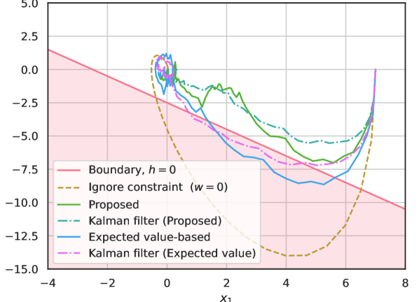
(a) Method 1

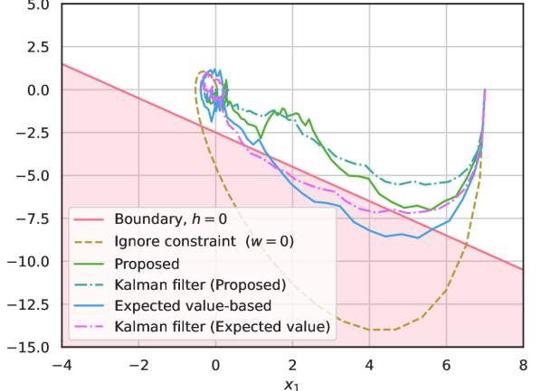
(b) Method 2

Figure 1: Phase portrait for vehicle navigation: the red regions indicate the unsafe region $h(x)<0$

VII Conclusions

This paper developed control approaches for discrete-time linear stochastic systems, where not all the states are directly observable. By employing the Kalman filter together with the worst-case CVaR, we effectively incorporated the tail risk into CBFs, thereby generating risk-aware constraints leading to the controller synthesis that effectively manage tail risks at the boundaries of safe sets for such systems. Two distinct control methods, designed for half-space and ellipsoidal safe sets, were discussed in detail, respectively. Numerical examples demonstrated improved safety and reliability in managing stochastic uncertainties, showcasing their applicability in real-world scenarios.

The proposed approaches contribute to the field of risk-aware control, offering a foundation for future research in enhancing safety measures. Future research directions include expanding these techniques to nonlinear systems and networked control systems, broadening their scope and impact.

References

• [1] P. Wieland and F. Allgöwer, “Constructive safety using control barrier functions,” IFAC Proc. Volumes, vol. 40, no. 12, pp. 462–467, 2007.
• [2] A. Agrawal and K. Sreenath, “Discrete control barrier functions for safety-critical control of discrete systems with application to bipedal robot navigation,” Robotics: Science and Systems, 2017.
• [3] A. D. Ames, J. W. Grizzle, and P. Tabuada, “Control barrier function based quadratic programs with application to adaptive cruise control,” in IEEE Conf. on Decision and Control, 2014, pp. 6271–6278.
• [4] J. Breeden and D. Panagou, “Guaranteed safe spacecraft docking with control barrier functions,” IEEE Control Systems Letters, vol. 6, pp. 2000–2005, 2022.
• [5] J. Seo, J. Lee, E. Baek, R. Horowitz, and J. Choi, “Safety-critical control with nonaffine control inputs via a relaxed control barrier function for an autonomous vehicle,” IEEE Robotics and Automation Letters, vol. 7, no. 2, pp. 1944–1951, 2022.
• [6] A. Clark, “Control barrier functions for stochastic systems,” Automatica, vol. 130, p. 109688, 2021.
• [7] C. Wang, Y. Meng, S. L. Smith, and J. Liu, “Safety-critical control of stochastic systems using stochastic control barrier functions,” in IEEE Conf. on Decision and Control, 2021, pp. 5924–5931.
• [8] R. K. Cosner, P. Culbertson, A. J. Taylor, and A. D. Ames, “Robust safety under stochastic uncertainty with discrete-time control barrier functions,” 2023, https://arxiv.org/abs/2302.07469.
• [9] W. Luo, W. Sun, and A. Kapoor, “Multi-robot collision avoidance under uncertainty with probabilistic safety barrier certificates,” in Advances in Neural Information Processing Systems, H. Larochelle, M. Ranzato, R. Hadsell, M. Balcan, and H. Lin, Eds., vol. 33.   Curran Associates, Inc., 2020, pp. 372–383.
• [10] S. Yaghoubi, K. Majd, G. Fainekos, T. Yamaguchi, D. Prokhorov, and B. Hoxha, “Risk-bounded control using stochastic barrier functions,” IEEE Control Systems Letters, vol. 5, no. 5, pp. 1831–1836, 2021.
• [11] M. Ahmadi, X. Xiong, and A. D. Ames, “Risk-averse control via CVaR barrier functions: Application to bipedal robot locomotion,” IEEE Control Systems Letters, vol. 6, pp. 878–883, 2022.
• [12] M. Kishida, “A risk-aware control: Integrating worst-case CVaR with control barrier function,” 2023, https://arxiv.org/abs/2308.14265.
• [13] A. Singletary, M. Ahmadi, and A. D. Ames, “Safe control for nonlinear systems with stochastic uncertainty via risk control barrier functions,” IEEE Control Systems Letters, vol. 7, pp. 349–354, 2023.
• [14] A. Clark, “Control barrier functions for complete and incomplete information stochastic systems,” in American Control Conference, 2019, pp. 2928–2935.
• [15] E. Daş and R. M. Murray, “Robust safe control synthesis with disturbance observer-based control barrier functions,” in IEEE Conf. on Decision and Control, 2022, pp. 5566–5573.
• [16] Y. Wang and X. Xu, “Observer-based control barrier functions for safety critical systems,” in American Control Conference, 2022, pp. 709–714.
• [17] D. R. Agrawal and D. Panagou, “Safe and robust observer-controller synthesis using control barrier functions,” IEEE Control Systems Letters, vol. 7, pp. 127–132, 2023.
• [18] S. Yaghoubi, G. Fainekos, T. Yamaguchi, D. Prokhorov, and B. Hoxha, “Risk-bounded control with kalman filtering and stochastic barrier functions,” in IEEE Conf. on Decision and Control, 2021, pp. 5213–5219.
• [19] R. E. Kalman, “A New Approach to Linear Filtering and Prediction Problems,” J. of Basic Engineering, vol. 82, no. 1, pp. 35–45, 1960.
• [20] G. Welch and G. Bishop, “An introduction to the kalman filter,” 1995.
• [21] S. Zhu and M. Fukushima, “Worst-case conditional value-at-risk with application to robust portfolio management,” Operations research, vol. 57, no. 5, pp. 1155–1168, 2009.
• [22] S. Zymler, D. Kuhn, and B. Rustem, “Distributionally robust joint chance constraints with second-order moment information,” Mathematical Programming, vol. 137, pp. 167–198, 2013.
• [23] R. T. Rockafellar and S. Uryasev, “Optimization of conditional value-at-risk,” J. of Risk, vol. 2, pp. 21–41, 2000.
• [24] A. Shapiro and A. Kleywegt, “Minimax analysis of stochastic problems,” Optimization Methods and Software, vol. 17, no. 3, pp. 523–542, 2002.
• [25] P. Artzner, F. Delbaen, J.-M. Eber, and D. Heath, “Coherent measures of risk,” Mathematical Finance, vol. 9, pp. 203–228., 1999.
• [26] S. Zymler, D. Kuhn, and B. Rustem, “Worst-case value at risk of nonlinear portfolios,” Management Science, vol. 59, no. 1, pp. 172–188, 2013.
• [27] J. Zeng, B. Zhang, and K. Sreenath, “Safety-critical model predictive control with discrete-time control barrier function,” in 2021 American Control Conference (ACC), 2021, pp. 3882–3889.
• [28] A. D. Ames, X. Xu, J. W. Grizzle, and P. Tabuada, “Control barrier function based quadratic programs for safety critical systems,” IEEE Trans. on Automatic Control, vol. 62, no. 8, pp. 3861–3876, 2017.
• [29] A. D. Ames, S. Coogan, M. Egerstedt, G. Notomista, K. Sreenath, and P. Tabuada, “Control barrier functions: Theory and applications,” in European Control Conference, 2019, pp. 3420–3431.
• [30] A. D. Ames and M. Powell, Towards the Unification of Locomotion and Manipulation through Control Lyapunov Functions and Quadratic Programs.   Heidelberg: Springer International Publishing, 2013, pp. 219–240.