High count rate effects in event processing for XRISM/Resolve x-ray microcalorimeter

Abstract

The spectroscopic performance of x-ray instruments can be affected at high count rates. The effects and mitigation in the optical chain, such as x-ray attenuation filters or de-focusing mirrors, are widely discussed, but those in the signal chain are not. Using the Resolve x-ray microcalorimeter onboard the XRISM satellite, we discuss the effects observed during high count rate measurements and how these can be modeled. We focus on three instrumental effects that impact performance at high count rate: CPU limit, pile up, and electrical cross talk. High count rate data were obtained during ground testing using the flight model instrument and a calibration x-ray source. A simulated observation of GX 13+1 is presented to illustrate how to estimate these effects based on these models for observation planning. The impact of these effects on high count rate observations is discussed.

1 Introduction

X-ray microcalorimeter is a device to convert the energy of incoming x-ray photons into heat and sense the temperature change of the thermometer cooled at a sub-K temperature[1]. This achieves unprecedented energy resolution over a wide energy range non-dispersively. Composing an array with multiple microcalorimeter pixels at a focus of an x-ray telescope further provides imaging capability, high signal-to-noise ratio, and wide dynamic range. The device is anchored to a thermal bath with a time constant of $\mathcal{O}(1~{}\textrm{ms})$. The signals are sampled at $\mathcal{O}(10~{}\textrm{kHz})$ and the entire time-resolved pulse shape is used to derive the energy of individual x-ray events.

At high count rates, the superb spectroscopic performance of the XRISM/Resolve instrument can be affected due to a variety of effects, some of which are discussed here. First, x-ray pulses overlap each other due to the slow thermal time constant. Second, for space applications, signal processing is performed onboard and only the characteristic values of pulses are downlinked to fit into the telemetry bandpass[2]. Computational resources can limit the rate of processing. These non-linear effects are further complicated by cross talks among multiple pixels. The only example of high count rate astrophysical observations is the Crab [3] with the soft x-ray spectrometer (SXS)[4] onboard ASTRO-H [5] in 2016. The x-ray spectrum is too featureless to leave a striking impact to the community. The purpose of this paper is to present a case study of such limitations and mitigation using the x-ray microcalorimeter Resolve[6] (Ishisaki et al. in this volume) onboard XRISM [7] by combining experimental and simulation methods. Preceding papers discussed the mitigation made in the optical chain such as an x-ray attenuation filter[8] or the de-focusing mirrors[9]. We focus on the signal chain.

We start with Figure 1 where we simulate some of the effects of high count rate observations with Resolve. An x-ray spectrum is simulated for GX 13$+$1, a low mass x-ray binary (LMXB), observed with Resolve near the array center using a 1/4 neutral density (ND) filter. The Fe Ly$\alpha^{1,2}$ absorption features with an assumed turbulent velocity of $v_{\mathrm{turb}}=200$ km s^-1 are shown (see § 4.2 for details of the fitting model). As we will see in this paper, the cross talk degrades the energy resolution as the flux increases. Without taking this effect into account, one can easily obtain an artificial flux dependence of $v_{\mathrm{turb}}$ (Figure 1 d) and may give a wrong astrophysical interpretation, such as the turbulent motion in the outflowing gas becomes more significant in the brighter phase.

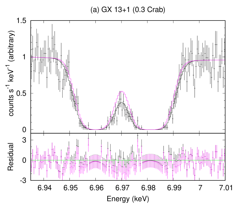
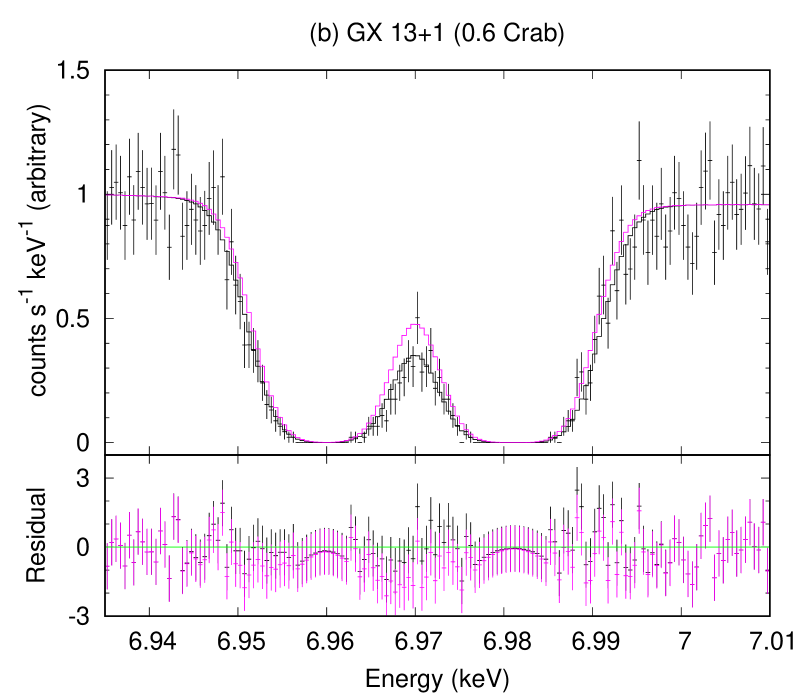
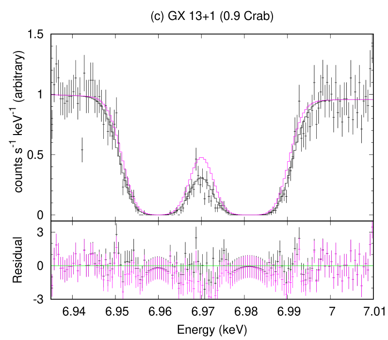
Figure 1: (a)-(c) Simulated spectra of GX 13$+$1 at three different assumed count rates. The vertical axis is normalized at 6.935 keV. Magenta curve shows the input spectrum for the simulation and the black lines are the resultant simulated spectra by including the cross-talk degradation. If the spectra are fitted without considering this effect as shown with the black curve, the estimate of the turbulent velocity has an increasing systematics as a function of the count rate, resulting in a fake correlation between the two in (d).

For proper observation planning and data analysis, such behaviors need to be described and modeled based on actual data taken under controlled setup, which will be discussed in this paper with the following plan. In § 2, we give a brief description of the Resolve instrument focusing on the topics related to this study. In § 3, we discuss the experimental part of this work. We focus on three effects in the signal chain: (1) CPU limit, (2) pulse pile-up, and (3) spectral degradation by electrical cross talk. The data acquisition (§ 3.1) and analysis (§ 3.2) using the hardware and software for flight are shown, and the experimental results of event loss and spectral distortion is discussed (§ 3.3). In § 4, we discuss the simulation part, first for modeling these effects (§ 4.1) and presenting a case study in astrophysical application (§ 4.2). The paper is summarized in § 5. Throughout this paper, we use a conversion of 2.14 s^-1 array^-1 for a point-like source of a mCrab flux placed at one of the center pixels to put the hardware limitations into astrophysical contexts. We note that the thermal effects at high count rates are not included in this paper.

2 Instrument

The x-ray microcalorimeter for Resolve is based on the ion-implanted Si thermometers with HgTe x-ray absorbers anchored to a 50 mK heat sink with a thermal time constant of $\sim$3.5 ms. An array consists of 6$\times$6 pixels (pixel 0–35)[10], below which an anti-coincidence detector[11] (anti-co) with two readouts is placed for identifying cosmic-ray events. One of the 36 pixels (pixel 12) is displaced from the array to be illuminated by an ⁵⁵Fe source for gain tracking common to the entire array. The thermometer resistance of $\sim$30 M$\Omega$ is read out individually for each pixel, which is converted to low impedance with the junction field effect transistor (JFET) amplifiers to go outside of the cryostat. The JFET operates at 130 K, thus needs to be placed physically apart from the 50 mK stage[12]. The cross talk takes place between adjacent channels in the high impedance part of the circuit prior to the JFET trans-impedance amplifiers. The pixels are enumerated by the wire layout of this part, so the pixel $i$ cross-talks to pixels $i\pm 1$ with a peak pulse height of 0.6% (relative physical pulse height before optimal filtering), and $i\pm 2$ with 0.1% in the same CPU board.

The signals are sampled at 12.5 kHz with a bipolar 14 bit ADC in the onboard analog electronics (XBOX)[12], which is relayed to the onboard digital electronics (Pulse Shape Processor; PSP)[13] for event detection and reconstruction. The PSP consists of two identical units (PSP-A and PSP-B), each of which has one FPGA, two CPU, and one power supply boards. The FPGA boards are responsible for event candidate detection, while the CPU boards are for deblending overlapping events, grading them, and applying the optimum filtering. The four CPU boards (called PSP-A0, A1, B0, and B1) processes nine pixels consisting of a quadrant of the array. All channels are processed in parallel and all cross-channel processing is applied in the ground.

The CPU board uses an SH4-compatible 32-bit RISC processor at a clock speed of 60 MHz developed by the Mitsubishi Heavy Industries. TOPPERS is used for the real-time operating system. When a CPU hits 100% usage at $\sim$50 s^-1 quadrant^-1, the buffer storing event candidates or pulse waveforms for each pixel is cleared. The lost duration (start and stop) and the lost number of event candidates are downlinked as the lost event telemetry. The processing of the nine pixels are scheduled by a round robin with no priority for any pixels. Therefore, the pixels at the center suffer the event loss more often than the pixels in the periphery of the array for observations of point sources focused at the array center by the mirror with a half-power diameter (HPD) of 1.2–1.3 arcmin (2.4 pixels)[14].

The CPU consumption rate is a non-linear function of the count rate. Events are graded into high, med, and low (H, M, or L) resolution depending on how close they are in time to an adjacent event of the same pixel[2]. They are further sub-divided into primary (p) or secondary (s) for those without and with a preceding events. For HR ($=$Hp) / MR ($=$Mp$+$Ms) events, the template of a 1024/256 sample length (81.92/20.48 ms) is used for optimum filtering for deriving the characteristic values of an event, including the arrival time, energy, DERIV_MAX and RISE_TIME. DERIV_MAX is the maximum value of the derivative, and RISE_TIME is the time in units of 20 $\mathrm{\SIUnitSymbolMicro}\mathrm{s}$ from DERIV_MAX to zero-crossing of derivative, corresponding to the rise time of the raw pulse. For LR ($=$Lp$+$Ls) events, only coarse values of these characters are derived based on the FPGA. As the count rate increases, the resource-demanding Hp events decreases and non-demanding Ls events increase. Depending on the spectral hardness, the spurious events caused by low energy redistribution can become non-negligible for resource usage.

3 Experiments

3.1 Data acquisition

We obtained the high count rate data at the instrument-level test in the Tsukuba Space Center of JAXA in 2022 February 20–21 (Figure 2). The flight model hardware and optimum filtering templates were used. The instrument was run in the cryogen-free mode. One configuration difference from the flight is the insertion of the data repeater between XBOX and PSP. All incoming data from XBOX are intercepted and copied to a PC, in which the PSP-equivalent processing was run in parallel with the PSP using a software (called SCDP) with virtually no CPU limits. This is the highest level of integration with the data repeater; no similar data can be taken after this experiment both on the ground and in the orbit.

We utilized the x-ray sources developed for the ground calibration of the gain curve (RTS; rotating target source)[15]. X-rays are generated by fluorescence of a selected target. The x-ray was illuminated uniformly beyond the array, causing some fluctuation in the thermal bath. This is not realistic for actual observations as high count rate effects matter only for bright point sources with counts concentrated at the array center. The difference is considered in the simulation (§ 4).

The high voltage current was controlled step-wise to have the count in the 0.4–14.5 s^-1 pixel^-1 range for a 10–30 min exposure (Table 3 and Figure 3).

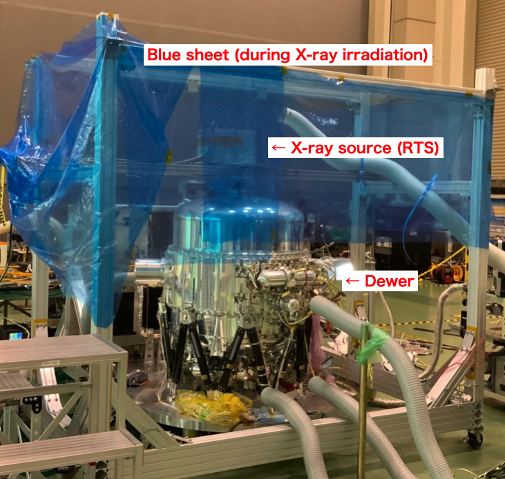
Figure 2: Photo of the experimental setup.

Step	Line	Current	Exposure
		($\mathrm{\SIUnitSymbolMicro A}$)	(min)
1	Ni	12	10
2		200	30
3		12	10
4		131	30
5		12	10
6		102	10
7		88	10
8		12	10
9		73	10
10		58	10
11		12	10
12		44	10
13		29	10
14		12	10
15		9	20
16		5	20
17		12	10
18	KBr	12	10
19		120	30
20		12	10
21		6	15

Table 1: Experimental setup for each step.

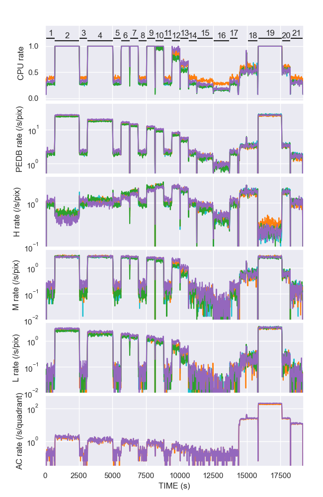
Figure 3: (from top to bottom) Rate of CPU consumption, FPGA-detected event candidate, HR, MR, LR, and anti-co events for each CPU in different colors. The steps in Table 3 are shown at the top.

3.2 Data reduction & analysis

The data were processed as flight-like as possible using the pre-pipeline[16] and pipeline[17] processing developed for the in-orbit data. We made some modifications to be compatible with the instrument-level test data that have no orbit and spacecraft information. The gain curve was implemented in the calibration data base for the cryogen-free operation[18]. The screening criteria that are standard in ASTRO-H SXS were applied. The common-mode gain was corrected using the ⁵⁵Fe source illuminating the pixel 12. The X-ray irradiation of the array at high count rates causes thermal effects on each pixel, which changes the gain scale. To correct this effect phenomenologically in the Ni illumination data (step 1–17), a spectrum was created for each pixel at each step, and the gain scale was corrected so that the Ni K$\alpha$ emission line center is at the correct energy. Correction methods for such thermal effects will be discussed in a subsequent paper. The Ni data are used for the assessment of the cross-talk degradation (§ 3.3.3), while both the Ni and KBr data are for all the assessments (§ 3.3.1–§ 3.3.3).

3.3 Results

3.3.1 CPU limit

Resolve has the requirement of processing the count rate of $>$200 s^-1 array^-1, including background and spurious events, without loss of events. This is called the PSP limit. We first verify that Resolve meets this requirement. From Figure 3, the CPU consumption rate is clipped at 100% for the steps with $I>73$ $\mathrm{\SIUnitSymbolMicro A}$ for the Ni data and $I=120$ $\mathrm{\SIUnitSymbolMicro A}$ for KBr. The average rate of these steps is 50.76, 46.58, 50.91, and 53.15 s^-1 quadrant^-1 respectively for PSP-A0, A1, B0, and B1. The total of 201.4 s^-1 array^-1 meets the requirement. About 76% of them are cleaned events for astrophysical use.

Table 2: PSP processed rate per pixel (1=HR, 2=MR, 3=LR, 4=Total, 5=cleaned events total, 6=cleaned events total corrected for the dead time), dead time percentage (7), and SCDP processed rate (8). (6)/(8) shows the efficiency due to the pile-up effect. The values for PIXEL 0 are shown.

Step	PSP processed rate						Dead time fraction	SCDP processed rate	(6)/(8)
	(1)	(2)	(3)	(4)	(5)	(6)	(7)	(8)
2	0.46	2.64	2.59	5.69	4.59	14.75	0.69	15.32	0.96
4	0.90	2.77	1.96	5.63	4.40	10.43	0.58	10.43	1.0
6	1.40	2.52	1.59	5.51	4.46	8.49	0.48	8.52	1.0
7	1.40	2.51	1.56	5.48	4.07	7.45	0.45	7.30	1.0
9	1.75	2.43	1.46	5.63	3.99	5.96	0.33	5.97	1.0
10	2.65	2.41	1.16	6.21	4.75	4.75	0.00	4.76	1.0
12	2.45	1.73	0.78	4.95	3.68	3.68	0.00	3.68	1.0
13	2.03	0.74	0.25	3.03	2.54	2.54	0.00	2.55	1.0
14	1.19	0.21	0.07	1.48	1.05	1.05	0.00	1.03	1.0
15	0.84	0.08	0.05	0.98	0.76	0.76	0.00	0.76	1.0
16	0.50	0.03	0.01	0.55	0.42	0.42	0.00	0.43	1.0
19	0.36	2.56	2.94	5.86	3.15	10.77	0.71	10.97	0.98
20	1.57	0.32	0.18	2.07	1.06	1.06	0.00	1.06	1.0
21	0.73	0.11	0.17	1.00	0.46	0.46	0.00	0.46	1.0

We next examine if the count rate beyond the PSP limit can be corrected using the lost event telemetry. Figure 4 shows an example of the dead time for two selected pixels (0 and 1), each of which has a count rate of 14.75 and 14.28 s^-1 pixel^-1 and a dead time fraction of 45% and 31%, respectively. The actual count rate can be derived by compensating for the dead time, which is available in the lost event telemetry. The pixel count rates thus corrected are summed for the array count rate, which is compared to the SCDP result in Table 2. The count rate is recovered even when the dead time fraction is large within a few percent.

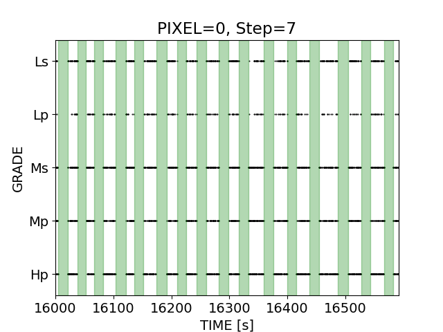
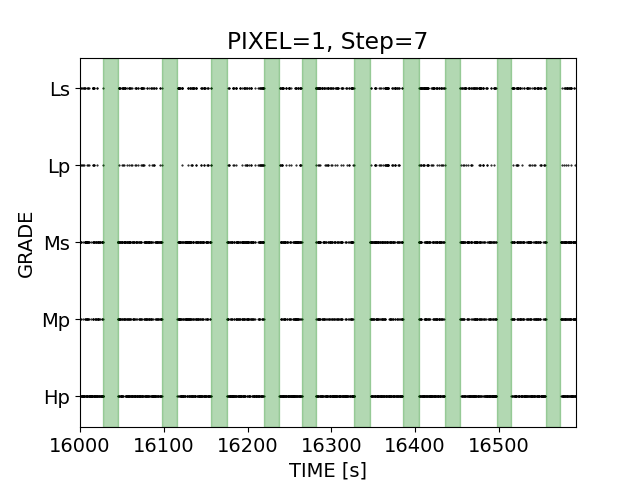
Figure 4: Example of the pixel dead time in PSP. Two pixels (0 and 1 with a count rate of 14.75 and 14.28 s^-1 pixel^-1, respectively) in the step 7 in Table 3 have dead times shown with green shades, during which all events are discarded. Dots shows the grade and the arrival time of each event.

3.3.2 Pile-up

The CPU subtracts the scaled average pulse shape from primary events and search for overlapping pulses to detect secondary events. If the overlapping pulses are too close in time, they are not distinguished and treated as one event, which we call pile-up. Similarly to the CCD pile-up, this distorts the spectrum and the count rate. For line-dominated x-ray spectrum such as the one presented here, the pile-up is most evident in the spectrum at an energy twice of the line (Figure 5).

For astrophysical spectra with line as well as continuum emission, the double energy spectrum would not be so obvious that we cannot apply the energy cut for screening. We thus use the distribution of the RISE_TIME versus energy relation. RISE_TIME indicates how fast a pulse reaches its peak in time, which is related to the energy. Pile-up events deviates from the normal trend (Figure 7), based on which we can remove pile-up events. In addition, we screened the event using SLOPE_DIFFER; events the slope of the derivative of which is different from the average one are discarded[13]. After applying the screening, we found that the pile-up spectrum improved (Figure 5), though not all pile-up events were completely removed for the overlapping distribution in Figure 7.

We now estimate the dead time caused by not detecting the overlapping pulse too close in time. The PSP software is designed to detect two pulses separated by $>$6 ms for all, and $>$2 ms if the peak contrast from the secondary to the primary events is $>$20. This is seen by using the Lp and Ls pairs in the actual data. Figure 7 shows the difference of time and the contrast of a proxy of the pulse height (DERIV_MAX) of Lp–Ls pairs. The contrast is bimodal for the line-dominated spectrum and its cross talk, but the boundaries of 2 and 6 ms are evident. Let’s assume that the average count rate of $\nu$ s^-1 pixel^-1 fluctuates following the Poisson distribution. The fraction of events arriving within $\Delta t_{\mathrm{thres}}$ of the preceding pulse is $\exp(-2\nu\Delta t_{\mathrm{thres}})$. For $\nu=15$ s^-1 pixel^-1 and $\Delta t_{\mathrm{thres}}=$2 ms, the fraction of pile-up events, hence the loss of observing time by screening them, is 6%. We note that $\Delta t_{\mathrm{thres}}$ in SCDP is as small as $\sim 0.8$ ms.

Figure 5: X-ray spectra with Hp grade in step 2 in Table 3. The peaks around 7.5 keV and 15 keV show the energy of Ni K$\alpha$ and twice of it. The blue and orange lines show the spectrum before and after the screening in Figure 7, respectively.

Figure 6: Plots of RISE_TIME versus energy of all events observed in step 2 in Table 2. Screening criteria for x-ray events are shown with dashed curves $|\texttt{RISE\_TIME}-52+\textrm{Energy}*(52-42)/16383.75|\leq 4$ remove pile-up events seen at twice of the Ni K$\alpha$ energy.

Figure 7: Difference of arrival time (horizontal axis) and the contrast of the peak of Lp-Ls pairs. The TRIG_TIME is the triggered time based on the local crystal oscillator in PSP and its difference is used for the horizontal axis. All the data from step 1 to 21 in Table 2 are used.

3.3.3 Cross talk

The energy resolution was evaluated by fitting the Ni K$\alpha$ line with varying count rates. The spectrum in the 7440–7495 eV range was fitted with a five-Lorentzian model with the natural width[19] and the required Gaussian broadening was used for the energy resolution in FWHM. Figure 8 shows the result. The energy resolution degrades from 4.61 $\pm$ 0.06 to 7.17 $\pm$ 0.07 eV when the count rate increases from 0.91 to 14.5 s^-1 pixel^-1.

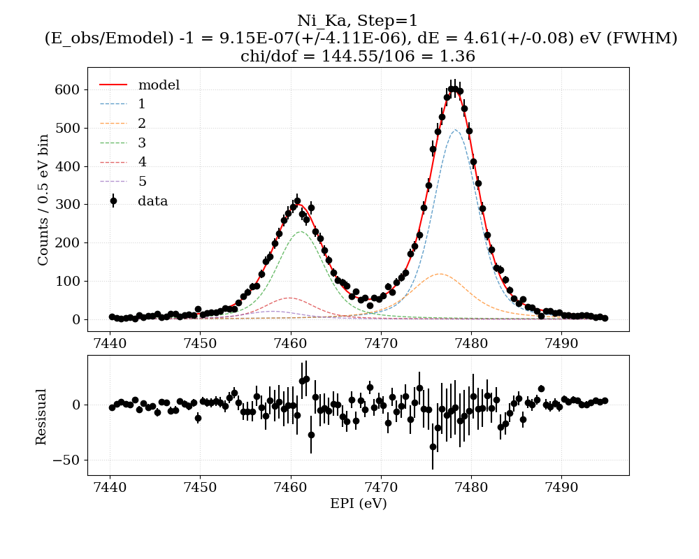
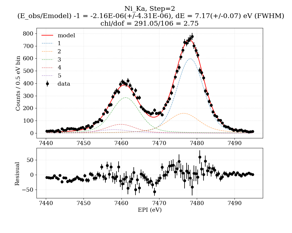
Figure 8: Fitting result of the Ni K$\alpha$ lines in step 1 (left) and 2 (right) in Table 2. The five Lorentzians (1–5) are shown with the dotted curves, while their sum is in the solid curve. The lower panel shows the residuals to the best fit.

Electrical cross talk is considered to be the major cause of the degradation. A part of the energy of a pulse (cross-talk parent) is deposited in the adjacent pixels (cross-talk children), which contaminates another pulse, if any, that would otherwise be uncontaminated. The optimum filtering is designed to mitigate this by reducing the weight for high frequency content, in which the cross-talk children is more enhanced for their capacitive coupling nature. Still, this leaves measurable effects when the count rate is high.

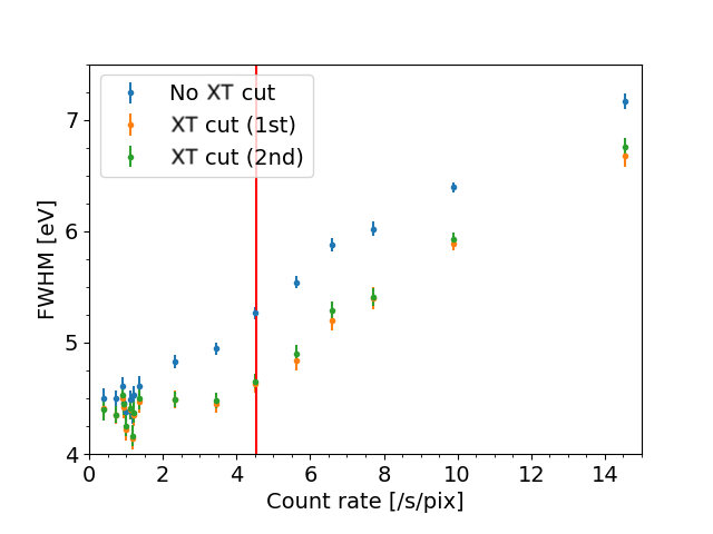
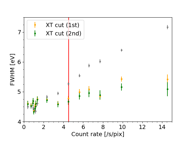
Figure 9: Energy resolution (FWHM) of the Ni K$\alpha$ lines as a function of the count rate using the PSP (left) and the SCDP (right) data. The blue, orange, and green data respectively indicate the results without the cross-talk cut, with the cut for the first and the second neighbors. The gray bins in the right panel are the same as the blue ones in the left panel. The red line shows the PSP limit.

The degradation is recovered by applying the cross-talk cut at a sacrifice of the effective exposure time. If a pulse in the pixel $i$ arrives within 25 ms of another pulse in the pixel $i\pm 1$ (first neighbors), it is discarded as being contaminated by the cross talk. The cut can be extended to $i\pm 2$ (second neighbors). Figure 9 shows the result, in which the energy resolution is shown against the count rate without the cross-talk cut (blue), with the cut for the first (orange) and the second (green) neighbors. For the PSP result (left), the resolution monotonically degrades, but is recovered by the cross-talk cut below the PSP limit of $\sim$4.5 s^-1 pixel^-1. The difference between the first and second neighbor cut is not significant. Beyond the PSP limit, this strategy works only partially, because the events are discarded and no cross-talk cut is available for its neighboring pixels. Figure 4 shows that the dead time (shown in green) depends on the pixel, because the count rate varies from pixel to pixel. If the cross-talk parent is within the dead time, we can no longer identify it. This is confirmed with the SCDP result (right), which does not suffer from such losses. The recovery of the resolution is seen beyond the PSP limit. The recovery is incomplete presumably because of the thermal bath fluctuation by the uniform x-ray illumination of the experiment (§ 3.1).

4 Simulation

In this section, we construct models to describe the high count rate effects (§ 4.1). The models are intended for observation planning, thus are phenomenological. In combination with the event simulator in the HEAsoft package, observers can assess the level of high count rate effects with the presented models as exemplified in § 4.2.

4.1 Models describing high count rate effects

4.1.1 CPU limit

For the CPU limit, we model the PSP’s CPU consumption rate. We assume that the rate is proportional to the incoming count rate of each grade (HR, MR, and LR) plus the base load. The four CPUs (A0, A1, B0, and B1) are not completely identical in their loads: A1 and B1 are responsible for communicating with the XBOX, while A0 and A1 are for processing the anti-co data. A1 receives counts from pixel 12 that produces $\sim$10 s^-1 pixel^-1 of the ⁵⁵Fe calibration source. In addition, all CPUs process baseline events, in which optimum filtering is applied to the noise records for diagnostic purposes.

The CPU consumption rate is modeled as a linear combination of these rates.

$$\textrm{(CPU rate)}^{\mathrm{(c)}}=\sum_{\mathrm{pixel}}\,a_{k}^{\mathrm{(c)}}*(\textrm{pixel count rate of the event type }k)+c^{\mathrm{(c)}},$$ (1)

where $k$ is Hp, Mp, Ms, Lp, Ls, baseline, and anti-co events, and $c$ is A0, A1, B0 and B1. All these information is available from the PSP telemetry. We used the Ni data in Table 2 during periods with the CPU consumption rate of 5–95% to determine the coefficients (Table 3). The best-fit model matches well with the observation (Figure 10 left panel). For verification, we applied the model to the KBr data (Figure 10 right panel), showing a good match as well. The result shows that the base load is 7–9%, and each x-ray event consumes 1.5–2.0% depending on the grade. The consumption due to the baseline and anti-co events are negligible.

Table 3: Fitting results of the CPU load fraction

CPU	A0	A1	B0	B1
Pixel	0–8	9–17	18–26	27–35
$a_{\textrm{Hp}}$	0.0197	0.0193	0.0199	0.0195
$a_{\textrm{Mp}}$	0.0180	0.0166	0.0194	0.0199
$a_{\textrm{Ms}}$	0.0174	0.0178	0.0170	0.0153
$a_{\textrm{Lp}}$	0.0221	0.0168	0.0174	0.0178
$a_{\textrm{Ls}}$	0.0147	0.0157	0.0163	0.0152
$a_{\textrm{BL}}$	0.0002	0.0000	0.0001	0.0001
$a_{\textrm{antico}}$	—	0.0005	—	0.0002
$c$	0.0842	0.0972	0.0834	0.0787

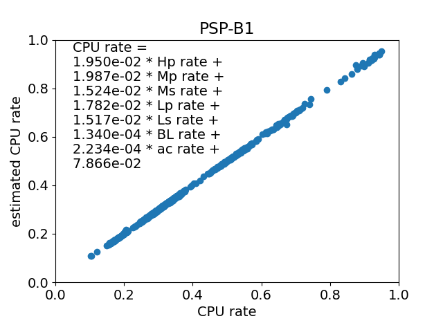
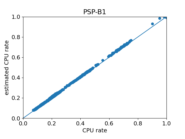
Figure 10: Result of CPU consumption model using the Ni data (left) and the application of the model to the KBr data (right). The result for the B1 CPU is shown. The measured CPU rates are plotted against the CPU rate calculated by the model.

4.1.2 Pile-up

Assuming the 1.3 arcmin HPD of the mirror[14] and the effective time ratio of $\exp(-2\nu\Delta t_{\mathrm{thres}})$ (see § 3.3.2), the effective time reduced by the pile-up effect on the entire array can be calculated. Figure 11 shows the ratio of the effective exposure time ($\alpha_{\mathrm{noPileUp}}$) as a function of the x-ray flux ($f_{\mathrm{X}}$ [mCrab]), with $\Delta t_{\mathrm{thres}}=2$ ms. The phenomenological fitting results in $\alpha_{\mathrm{noPileUp}}=\exp(-f_{\mathrm{X}}/959)*(1-1.055\times 10^{-4}f_{\mathrm{X}}+4.842\times 10^{-7}{f_{\mathrm{X}}}^{2})$. Note that this relation is valid only up to 2 Crab.

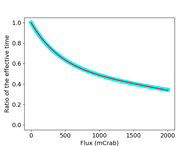
Figure 11: Ratio of the effective exposure time reduced by the pile-up effect as a function of the x-ray flux. The cyan shows the simulation results, whereas the red is the phenomenological fitting.

4.1.3 Cross talk

We model the behavior of the cross-talk effect as a function of the count rate. First, we derive how the line broadening is recovered by the cross-talk cut as

$$\mathrm{FWHM_{recovery}}=(\mathrm{FWHM_{NoXTalkCut}}^{2}-\mathrm{FWHM_{XTalkCut}}^{2})^{1/2},$$ (2)

in which $\mathrm{FWHM_{NoXTalkCut}}$ and $\mathrm{FWHM_{XTalkCut}}$ are the energy resolution in FWHM without and with the cross-talk cut. Here, we attribute the excess broadening in $\mathrm{FWHM_{XTalkCut}}$ from the intrinsic FWHM of 4.6 eV to the thermal bath fluctuation due to inappropriate setting in the experiment (§ 3.1), which would not be so evident in actual point source observations. Figure 13 shows the $\mathrm{FWHM_{recovery}}$ values as a function of the ratio of the cross-talk contaminated events to the total ($\beta_{\mathrm{XTalk}}$). For simplicity, we assume that an x-ray source uniformly illuminates all the pixels and that all the pixels share the same $\mathrm{FWHM_{recovery}}$. The $\beta_{\mathrm{XTalk}}$ value can be obtained through the use of public tools described later (§ 4.2). The $\mathrm{FWHM_{recovery}}$ is modeled as a reverse function of $\beta_{\mathrm{XTalk}}$ as

$$a*\mathrm{FWHM_{recovery}}^{2}+b*\mathrm{FWHM_{recovery}}=\beta_{\mathrm{XTalk}},$$ (3)

where $(a,\,b)=(0.125,\,0.054)$ for the 1st cross-talk cut and $(0.208,\,0.261)$ for the 1st+2nd cross-talk cut. This equation describes the data well (Figure 13).

The exposure time is lost by the cross-talk cut. Under the same situation as § 4.1.2, the ratio of the effective exposure time ($\alpha_{\mathrm{XTalk}}=1-\beta_{\mathrm{XTalk}}$) is calculated (Figure 13). The phenomenological fitting results in $\alpha_{\mathrm{XTalk}}=\exp(-f_{\mathrm{X}}/613)*(1-2.358\times 10^{-4}f_{\mathrm{X}}+6.919\times 10^{-7}{f_{\mathrm{X}}}^{2})$ for the 1st cross-talk cut, and $\alpha_{\mathrm{XTalk}}=\exp(-f_{\mathrm{X}}/226)*(1-2.538\times 10^{-3}f_{\mathrm{X}}+5.602\times 10^{-6}{f_{\mathrm{X}}}^{2})$ for the 1st+2nd cross-talk cut.

The count rate and the cross-talk contaminated event rate were calculated and the $\mathrm{FWHM_{recovery}}$ were estimated in each pixel. From these values, the count-weighted average $\mathrm{FWHM_{recovery}}$ were estimated. Figure 14 shows the result. For example, when we observe the point source whose flux is 400 mCrab with the 1/4 ND filter (i.e., when the irradiated flux is 100 mCrab), the line distortion with FWHM of 3.0 eV is produced without the cross-talk cut. With the cross-talk cut the energy resolution is recovered but the exposure time is lost by 16.5% (1st) or 48.8% (2nd) (Figure 13).

Figure 12: $\mathrm{FWHM_{recovery}}$ as a function of the cross-talk contaminated event rate over the total rate ($\beta_{\mathrm{XTalk}}$) for each pixel. The recovery is estimated separately for the first and second cross-talk cuts. When the second cross talk is additionally cut, both of the ratio of the cross-talk contaminated events increases and $\mathrm{FWHM_{recovery}}$ increases. This means that the orange point moves toward upper right to the green one.

Figure 13: Ratio of the effective exposure time ($\alpha_{\mathrm{XTalk}}=1-\beta_{\mathrm{XTalk}}$) as a function of the x-ray flux after the cross-talk cut. The blue/cyan shows the simulation results and the orange/red is the phenomenological fitting for the 1st/1st+2nd cross-talk cut, respectively. The loss of the effective time due to the pile-up is not included. The result for the first cross-talk cut is shown, because the function for first+second share almost the same result.

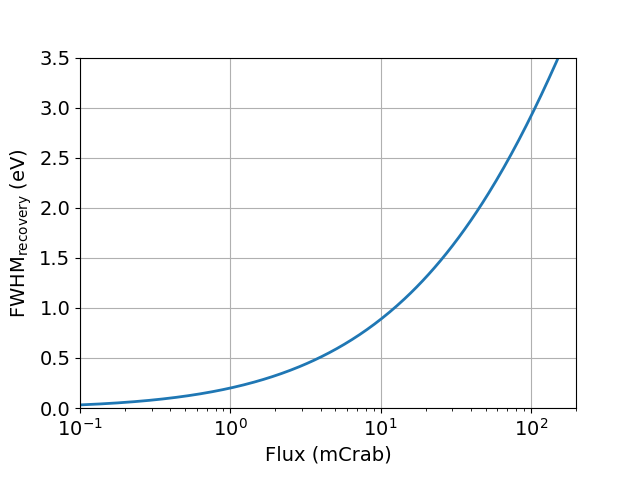
Figure 14: The $\mathrm{FWHM_{recovery}}$ of count-weighted average as a function of the X-ray flux (the reduced one if any filter is used). The X-ray source is assumed to be point like and with the same spectral distribution as Crab.

4.2 Simulated astrophysical observation

4.2.1 Input spectrum

We use GX 13$+$1 as a test case. The source is a LMXB hosting a neutron star (NS) and a low-mass companion with an orbital period of 24.5 days[20]. The x-ray flux varies around $\sim 0.3$ Crab. During dips, the soft band flux is reduced by $\sim$4 times [20]. The spectrum exhibits absorption by the ionized Fe and Ni K lines[21].

We start from the Chandra HETG observation with the ACIS operated in the continuous clocking mode (OBSID: 11818). The x-ray flux was 270 mCrab. We extracted the x-ray spectra and fitted them (Figure 16) using two continua (disk blackbody for the accretion disk and a blackbody for the NS surface emission) attenuated by the Galactic absorption and the local absorption by the ionized outflow. The H- and He-like Fe K absorption features are described using the kabs model[22]. The two absorption features are fitted with the absorption column of $8.9\times 10^{18}$ and $2.5\times 10^{17}$ cm^-2 (for each ion) with a common turbulent and outflow velocity respectively of 200 and $-330$ km s^-1. Constraining the absorption features is an important science goal of Resolve.

The mock event file was made using the heasim event simulator for the best-fit spectrum observed for 30 ks with the source placed at one of the center pixels (35). The flux is reduced by 1/4 assuming the use of the ND filter equipped with Resolve. Events above the energy threshold of 130.5 eV (DERIV_MAX $\sim$ 75) are extracted. The count rates of each grade in each pixel are calculated by rslbranch, which are shown in Figure 16. Over the entire array, the total, Hp, and Mp count rates are 62.5, 33.3, and 6.8 s^-1 array^-1, respectively. The branching ratio of the Hp events is 0.53. For each pixel, the total count rate varies from 16.1 (on-source position) to 0.2 s^-1 pixel^-1 (outer pixels) by nearly two orders. Overall, inner pixels cross-talk to outer pixels by design.

Figure 15: GX 13$+$1 spectrum observed with Chandra HETG and its best-fit model in the upper panel and the residuals to the fit in the lower panel. The black and red colors are for the $\pm$1st order dispersion data.

Figure 16: Distribution of count rate of the simulated Resolve observation. The pixel number is given in black, while the total, Hp, and Mp count rates (s-1 pixel-1) are in red, blue, and green texts, respectively.

4.2.2 Estimates of high count rate effects

CPU limit

The total count rate in the upper right quadrant (PSP-B1) is 33.46 s^-1 quadrant^-1, which is the highest by including the most illuminated pixel 35. The CPU consumption rate is calculated using Equation (1). Here, the anti-co and baseline counts are ignored (see § 4.1.1). The calculated CPU load is 0.306 (PSP-A0), 0.206 (A1) 0.307 (B0), and 0.667 (B1). Therefore, the event loss is not expected to occur in this observation.

Pile-up

The pile-up events are flagged in the heasim output file, with the parameter setting of dtpileup$=$0.002. The pile-up fraction, thus the loss of the effective exposure time, is calculated to be 2.5%.

Cross talk

We estimate the energy resolution degradation by the cross talk. The excess broadening $\mathrm{FWHM_{recovery}}$ of a pixel of interest increases when the neighboring pixels have high count rates. In the current simulation, the excess broadening is the largest in the pixel 34 and 33, which are the first and second neighbors of the most illuminated pixel 35. The effect needs to be estimated pixel by pixel, then summed for the array effect. We first derived the ratio of the cross-talk contaminated events ($\beta_{\mathrm{XTalk}}$ in Equation 3) based on the simulated event file. It was assumed that the effect of cross-talk contamination was present up to the second neighbor pixels. Next, using Equation (3), we estimated how much the resolution degrades for each pixel. The results are shown in Figures 18 and 18. Finally, we average the pixel degradation over the entire array weighted by the Hp count rate. The $\mathrm{FWHM_{recovery}}$ in the entire spectrum is estimated to be 1.59 eV at 7.5 keV. For a 5 eV resolution, the degraded resolution is estimated to be 5.25 eV.

Figure 17: Pixel map of the ratio of the cross-talk contaminated events: $\beta_{\mathrm{XTalk}}$ in Equation 3. The black shows the pixel number.

Figure 18: Pixel map of the excess broadening: $\mathrm{FWHM_{recovery}}$ in Equation 3. The black shows the pixel number.

4.2.3 Astrophysical impact

We visualized how the cross talk affects the observation. Figures 20 and 20 show the simulated spectra of GX 13+1, with a 30 ks exposure time at a flux of 270 mCrab and with the 1/4 ND filter. The spectra were created using the fakeit command in xspec, based on the best fitting model of the Chandra/HETG data (Figure 16). The black shows the spectrum when the cross-talk cut is not performed. The Hp response with 5 eV resolution was used, and the input model was artificially smoothed by the gsmooth model to mimic the line distortion due to the cross-talk effect. The red shows the one after the cross-talk cut. The model spectrum flux was reduced.

After the cross-talk cut, the resolution recovers but the apparent flux decreases. When the turbulent velocity of the absorption line is 200 km s^-1 and if the fitting is performed without recognizing the 1.59 eV excess broadening by the cross talk, the derived turbulent velocity becomes $\left(\left(200\mathrm{\,km\,s}^{-1}\right)^{2}+(1.59\mathrm{\,eV}/7477\mathrm{\,eV}\times c)^{2}\right)^{1/2}=210$ km s^-1, where $c$ is the light speed. If the cross-talk cut up to the second neighbor pixels are performed, the energy resolution will remain 5 eV at a sacrifice of the reduced Hp rate of 25.82 s^-1 array^-1, which is 77.5% of that without the cut. The trade-off should be made for each science cases using the recipe presented here.

Figure 19: The simulated GX 13+1 spectra with Hp grade, based on the 5 eV energy resolution response. The black/red shows the spectra before/after the cross-talk cut, respectively. The lower panel shows the residuals between the simulated data and the model. Both of the first and second cross talk is cut. We adopt the total duration time as the exposure time.

Figure 20: Same as Figure 20, but only the energy band around the H-like Fe-K absorption lines are shown. The lower panel shows the data minus the folded model. The fitting result for the red spectrum shows $v_{\mathrm{turb}}=200$ km s-1 as expected, but the one for the black results in $v_{\mathrm{turb}}=210$ km s-1, if we do not notice the spectral distortion due to the cross talk.

The same simulation was repeated with different fluxes. If the flux is twice as large, the estimated CPU consumption rate is 1.21 on PSP-A1. In this case, the situation becomes worse. The event loss occurs and the number of events that can be processed is reduced by a factor of 1/1.21. In addition, all the cross talks cannot be identified and cross-talk cut cannot be applied completely. The total, Hp, and Mp count rate is 114.5, 43.6, and 12.6 s^-1 array^-1, respectively. The branching ratio of Hp becomes smaller. The Hp-count-weighted $\mathrm{FWHM_{distort}}$ is calculated to be 2.18 eV, and the derived turbulent velocity becomes $218$ km s^-1. If the flux is three times as large, the estimated CPU rate is 1.74 on PSP-A1. The total, Hp, and Mp count rate in the array is 146.2, 45.8, 16.0 cts/s, respectively. The Hp-count-weighted $\mathrm{FWHM_{recovery}}$ is calculated to be 2.55 eV, and the derived turbulent velocity becomes $225$ km s^-1 (Figure 1).

5 Summary

We have presented the results of both experimental and simulation studies using the XRISM/Resolve x-ray microcalorimeter investigating the effects at high count rates. Three effects in the signal chain were considered: CPU limit, pile-up, and electrical cross talk. Based on the ground test results, we have characterized and modeled the behavior of the instrument. We further performed a mock observation of GX 13+1 and illustrated that the high count rate effects are clearly observed in the spectra. Observers aiming for high count rate observations with XRISM/Resolve should be aware of the effects presented here, and these effects should be taken into consideration during observation planning and analysis.

For the point sources, when the X-ray flux exceeds $\sim$10 mCrab ($\sim$40 mCrab with the 1/4 ND filter), the line distortion appears without the cross-talk cut. The cross talk cut can recover the line distortion at the expense of exposure time. When the X-ray flux is $\sim 120$ mCrab ($\sim 500$ mCrab with the 1/4 ND filter), the count rate exceeds the PSP limit, resulting in GIT lost and making it impossible to identify all the cross-talk contaminated events. Therefore, the line distortion cannot be fully recovered.

- [1] McCammon, D., Moseley, S. H., Mather, J. C., and Mushotzky, R. F., “Experimental tests of a single‐photon calorimeter for x‐ray spectroscopy,” Journal of Applied Physics 56, 1263–1266 (sep 1984).
- [2] Boyce, K. R., Audley, M. D., Baker, R. G., Dumonthier, J. J., Fujimoto, R., Gendreau, K. C., Ishisaki, Y., Kelley, R. L., Stahle, C. K., Szymkowiak, A. E., and Winkert, G. E., “Design and performance of the ASTRO-E/XRS signal processing system,” in [EUV, X-Ray, and Gamma-Ray Instrumentation for Astronomy X ], Siegmund, O. H. and Flanagan, K. A., eds., Society of Photo-Optical Instrumentation Engineers (SPIE) Conference Series 3765, 741–750 (Oct. 1999).
- [3] Tsujimoto, M. et al., “In-flight calibration of Hitomi Soft X-ray Spectrometer. (3) Effective area,” PASJ 70 (mar 2018).
- [4] Mitsuda, K. et al., “Soft x-ray spectrometer (SXS): the high-resolution cryogenic spectrometer onboard ASTRO-H,” in [Space Telescopes and Instrumentation 2014: Ultraviolet to Gamma Ray ], Takahashi, T., den Herder, J.-W. A., and Bautz, M., eds., 9144, 91442A (jul 2014).
- [5] Takahashi, T. et al., “Hitomi (ASTRO-H) X-ray Astronomy Satellite,” Journal of Astronomical Telescopes, Instruments, and Systems 4(2), 1 – 13 (2018).
- [6] Ishisaki, Y. et al., “Resolve Instrument on X-ray Astronomy Recovery Mission (XARM),” Journal of Low Temperature Physics 193, 991–995 (dec 2018).
- [7] Tashiro, M. S. et al., “Status of x-ray imaging and spectroscopy mission (XRISM),” in [Space Telescopes and Instrumentation 2020: Ultraviolet to Gamma Ray ], den Herder, J.-W. A., Nakazawa, K., and Nikzad, S., eds., 11444, 176, SPIE (dec 2020).
- [8] Done, C. et al., “ASTRO-H White Paper - Low-mass X-ray Binaries,” arXiv e-prints , arXiv:1412.1164 (Dec. 2014).
- [9] Kammoun, E. S., Barret, D., Peille, P., Willingale, R., Dauser, T., Wilms, J., Guainazzi, M., and Miller, J. M., “The defocused observations of bright sources with Athena/X-IFU,” arXiv e-prints , arXiv:2205.01126 (May 2022).
- [10] Porter, F. S., Boyce, K. R., Chiao, M. P., Eckart, M. E., Fujimoto, R., Ishisaki, Y., Kilbourne, C. A., Leutenegger, M. A., and McCammon, D., “In-flight performance of the soft x-ray spectrometer detector system on Astro-H,” JATIS 4, 1 (feb 2018).
- [11] Kilbourne, C. A. et al., “The design, implementation, and performance of the Atro-H SXS calorimeter array and anti-coincidence detector,” in [Space Telescopes and Instrumentation 2016: Ultraviolet to Gamma Ray ], den Herder, J.-W. A., Takahashi, T., and Bautz, M., eds., 9905, 1144 – 1152, International Society for Optics and Photonics, SPIE (2016).
- [12] Kelley, R. L. et al., “The Astro-H high resolution soft x-ray spectrometer,” in [Space Telescopes and Instrumentation 2016: Ultraviolet to Gamma Ray ], den Herder, J.-W. A., Takahashi, T., and Bautz, M., eds., Society of Photo-Optical Instrumentation Engineers (SPIE) Conference Series 9905, 99050V (July 2016).
- [13] Ishisaki, Y. and Yamada, S., “In-flight performance of pulse-processing system of the ASTRO-H/Hitomi soft x-ray spectrometer,” JATIS 4, 1 (mar 2018).
- [14] Okajima, T. et al., “First peek of ASTRO-H Soft X-ray Telescope (SXT) in-orbit performance,” 99050Z (jul 2016).
- [15] Eckart, M. E. et al., “Calibration of the microcalorimeter spectrometer on-board the Hitomi (Astro-H) observatory (invited),” Review of Scientific Instruments 87, 11D503 (nov 2016).
- [16] Terada, Y. et al., “Detailed design of the science operations for the XRISM mission,” Journal of Astronomical Telescopes, Instruments, and Systems 7, 037001 (July 2021).
- [17] Loewenstein, M. et al., “The XRISM science data center: optimizing the scientific return from a unique x-ray observatory,” in [Space Telescopes and Instrumentation 2020: Ultraviolet to Gamma Ray ], den Herder, J.-W. A., Nakazawa, K., and Nikzad, S., eds., 11444, 286, SPIE (dec 2020).
- [18] Porter, F. S., Chiao, M. P., Eckart, M. E., Fujimoto, R., Ishisaki, Y., Kelley, R. L., Kilbourne, C. A., Leutenegger, M. A., McCammon, D., Mitsuda, K., Sawada, M., Szymkowiak, A. E., Takei, Y., Tashiro, M., Tsujimoto, M., Watanabe, T., and Yamada, S., “Temporal Gain Correction for X-ray Calorimeter Spectrometers,” Journal of Low Temperature Physics 184, 498–504 (jul 2016).
- [19] Hölzer, G., Fritsch, M., Deutsch, M., Härtwig, J., and Förster, E., “ and x-ray emission lines of the transition metals,” Phys. Rev. A 56, 4554–4568 (Dec 1997).
- [20] Iaria, R., Di Salvo, T., Burderi, L., Riggio, A., D’Aì, A., and Robba, N. R., “Discovery of periodic dips in the light curve of GX 13+1: the X-ray orbital ephemeris of the source,” A&A 561, A99 (Jan. 2014).
- [21] Sidoli, L., Parmar, A. N., Oosterbroek, T., and Lumb, D., “Discovery of complex narrow X-ray absorption features from the low-mass X-ray binary GX 13+1 with XMM-Newton,” A&A 385, 940–946 (Apr. 2002).
- [22] Tomaru, R., Done, C., Ohsuga, K., Odaka, H., and Takahashi, T., “The thermal-radiative wind in the neutron star low-mass X-ray binary GX 13 + 1,” MNRAS 497, 4970–4980 (Oct. 2020).