Clustered Switchback Experiments:
Near-Optimal Rates Under Spatiotemporal Interference

Abstract

We consider experimentation in the presence of non-stationarity, inter-unit (spatial) interference, and carry-over effects (temporal interference), where we wish to estimate the global average treatment effect (GATE), the difference between average outcomes having exposed all units at all times to treatment or to control. We suppose spatial interference is described by a graph, where a unit’s outcome depends on its neighborhood’s treatment assignments, and that temporal interference is described by a hidden Markov decision process, where the transition kernel under either treatment (action) satisfies a rapid mixing condition. We propose a clustered switchback design, where units are grouped into clusters and time steps are grouped into blocks and each whole cluster-block combination is assigned a single random treatment. Under this design, we show that for graphs that admit good clustering, a truncated exposure-mapping Horvitz-Thompson estimator achieves $\tilde{O}(1/NT)$ mean-squared error (MSE), matching an $\Omega(1/NT)$ lower bound up to logarithmic terms. Our results simultaneously generalize the $N=1$ setting of Hu & Wager (2022) (and improves on the MSE bound shown therein for difference-in-means estimators) as well as the $T=1$ settings of Ugander et al. (2013); Leung (2022). Simulation studies validate the favorable performance of our approach.

1 Introduction

Randomized experimentation, or A/B testing, is widely used to estimate causal effects on online platforms. Basic strategies involve partitioning the experimental units (e.g., users or time periods) into two groups randomly, and assigning one group to treatment ad the other to control. A key challenge in modern A/B testing is interference: From two-sided markets to social networks, interference between units complicates experimentation and makes it difficult to estimate the true effect of a treatment.

The spillover effect in experimentation has been extensively studied (Manski, 2013; Aronow et al., 2017; Li et al., 2021; Ugander et al., 2013; Sussman & Airoldi, 2017; Toulis & Kao, 2013; Basse & Airoldi, 2018; Cai et al., 2015; Gui et al., 2015; Eckles et al., 2017; Chin, 2019). A majority of these works assume neighborhood interference, where the spillover effect is constrained to the direct neighborhood of an individual as given by an interference graph. Under this assumption, Ugander et al. (2013) proposed a clustering-based design, and showed that if the growth rate of neighborhoods is bounded, then the Horvitz-Thompson (HT) estimator achieves an asymptotically optimal mean squared error (MSE) of $\tilde{O}(d/N)$, where $d$ is the maximum degree. As there are many settings in which interference extends beyond direct neighbors, Leung (2022) considers a relaxed assumption in which the interference is not restricted to direct neighbors, but decays as a function of the spatial distance between vertices with respect to an embedding of the vertices in Euclidean space. As a special case, if each vertex only interferes with vertices within distance $h$, then the HT estimator has an MSE of $O(h^{2}/N)$ under a suitable spatial clustering design.

Orthogonal to the spillover effect, the carryover effect (or temporal interference), where past treatments may affect future outcomes, has also been extensively studied. Bojinov et al. 2023 considers a simple model in which the temporal interference is bounded by a fixed window length. Other works model temporal interference that arises from the Markovian evolution of states, which allows for interference effects that can persist across long time horizons (Glynn et al., 2020; Farias et al., 2022; Hu & Wager, 2022; Johari et al., 2022; Shi et al., 2023). A commonly used approach in practice is to deploy switchback experiments: where the exposure of the entire system (viewed as a single experimental unit) alternates randomly between treatment and control for sufficiently long contiguous blocks of time such that the temporal interference around the switching points does not dominate. Under a switchback design, Hu & Wager (2022) shows that the difference-in-mean (DIM) estimator with an appropriately chosen burn-in period achieves an MSE of $\tilde{O}(T^{-2/3})$, assuming that the Markov chains are rapidly mixing. They also showed that this rate is optimal within the class of DIM estimators.

While the prior studies have either focused on only network interference or only temporal interference, there are many practical settings in which both types of interference are present. On the surface, handling spatio-temporal interference may seem straightforward, considering that (i) time can be regarded as an additional “dimension”, and (ii) these two types of interference have been well-explored separately. However, in most work on network interference, the potential outcomes at different units conditioned on the vector of treatment assignments are assumed to be deterministic or independent (e.g., Ugander et al. 2013; Leung 2022). In a Markovian setting, this assumption breaks down, since past outcomes are correlated to future outcomes even conditioned on the treatments due to state evolution.

We consider experimentation with spatio-temporal interference on a multi-vertex Markovian model that encapsulates both (i) the network interference between vertices by a given interference graph, and (ii) the temporal interference that arises from Markovian state evolutions. We assume that the outcome and state evolution of each vertex depends solely on the treatments of their immediate neighborhood (including themself), and that the state evolutions are independent across vertices conditioned on the treatments.

We show that for graphs that admit a good clustering, such as a growth restricted graph or a spatially embedded graph, a truncated HT estimator achieves $\tilde{O}(1/NT)$ MSE under a simple switchback design, assuming that the Markov chains are rapidly mixing as in Hu & Wager 2022. In the special case with $N=1$, our result shows that an HT-type estimator for switchback experiments can break the $O(T^{-1/3})$ barrier for DIM estimators shown in Hu & Wager 2022, achieving an asymptotically faster rate of convergence.

1.1 Our Contributions

For any partition (i.e., vertex clustering) $\Pi$, for a suitable block length $\ell$, we show that a truncated HT estimator achieves an MSE of $1/NT$ times a graph clustering-dependent quantity which is constant for low degree graphs that admit good clusterings, e.g., growth restricted graphs or spatially derived graphs. The significance of this result becomes apparent when compared with known results in the following ways.
1. Stronger: We provide a faster rate for “pure” switchback experiments. Specifically, for $N=1$, our MSE bound is $\tilde{O}(1/T)$, asymptotically lower than the $\tilde{O}(T^{-2/3})$ bound for difference-in-means estimators in Hu & Wager 2022.
2. Minimax Optimality: Our result is nearly optimal in both $N$ and $T$ up to a logarithmic factor. This follows since the MSE of any estimator with any design is $\Omega(1/NT)$, even without interference.
3. More General: Our result extends several known results for network interference to incorporate temporal interference. Specifically, our main result implies the following generalizations of existing results.
(i) Network interference. Assuming that the interference graph satisfies the $\kappa$-restricted growth condition (formally defined in Section 3.3) for some $\kappa=O(1)$, Ugander et al. (2013) showed that the HT estimator achieves an MSE of $\tilde{O}(d/N)$ for $T=1$, with a suitable partition (graph clustering). Our Corollary 3.10 generalizes this to $\tilde{O}(d/NT)$ in the presence of Markovian temporal interference.
(ii) Spatial interference. Under $h$-neighborhood interference (i.e., each vertex interferes with vertices within $h$ hops), Leung (2022) showed an $O(h^{2}/N)$ MSE for $T=1$. Our Corollary 3.12 generalizes this to $\tilde{O}(h^{2}/NT)$ in the presence of Markovian temporal interference.

Finally, we reiterate that our setting, even for $N=1$, can not be reduced to that of Leung 2022. While the rapid mixing property implies that the temporal interference decays exponentially across time, which seems to align with Assumption 3 from Leung 2022 , they critically use an assumption that the outcomes conditioned on the treatments are given by a non-random potential outcomes function. While their analysis can be modified for independently random outcomes, the outcomes in our Markovian setting are not independent across time even conditioned on treatments.

1.2 Related work

Experimentation is a broadly-deployed learning tool in e-commerce that is simple to execute (Kohavi & Thomke, 2017; Thomke, 2020; Larsen et al., 2023). As a key challenge, the violation of the so-called Stable Unit Treatment Value Assumption (SUTVA) has been viewed as problematic in online platforms (Blake & Coey, 2014).

Many existing work that tackles this problem assumes that interference is summarized by a low-dimensional exposure mapping and that units are individually randomized into treatment or control by Bernoulli randomization (Manski, 2013; Toulis & Kao, 2013; Aronow et al., 2017; Basse et al., 2019; Forastiere et al., 2021). Some work departed from unit-level randomization and introduced cluster dependence in unit-level assignments in order to improve estimator precision, including Ugander et al. 2013; Jagadeesan et al. 2020; Leung 2022, 2023, just to name a few.

There is another line of work that considers the temporal interference (or carryover effect). Some works consider a fixed bound on the persistence of temporal interference (e.g., Bojinov et al. 2023), while other works considered temporal interference arising from the Markovian evolution of states (Glynn et al., 2020; Farias et al., 2022; Johari et al., 2022; Shi et al., 2023; Hu & Wager, 2022). Apart from being limited to the single-vertex setting, many of these works differ from ours either by (i) focusing on alternative objectives, such as the stationary outcome (Glynn et al., 2020), or (ii) imposing additional assumptions, like observability of the states (Farias et al., 2022).

A related line of work in reinforcement learning concerns off-policy evaluation (OPE) (Jiang & Li, 2016; Thomas & Brunskill, 2016). The goal is, in spirit, similar to our problem: Evaluate the performance of a policy based on the data generated by another policy. However, these works usually require certain state observability assumptions, which are not needed in our work. Moreover, these works usually impose certain assumptions on the non-stationary, whereas the non-stationarity in our work is completely arbitrary. Finally, works in OPE focuses on rather general data-generating policies (beyond fixed-treatment policies) and estimands (beyond ATE), compromising the strengths of the results.

Although extensively studied separately and recognized for its practical significance, experimentation under spatio-temporal interference has received relatively limited attention in previous works. Recently, Ni et al. (2023) attempted to address this problem, but their approach assumes that the carryover effect is confined to just one period.

2 Model Setup and Experiment Design

Consider a horizon with $T$ rounds and $N$ vertices, where each vertex at each time is randomly assigned to treatment (“1”) or control (“0”). We model the interference between vertices using an interference graph $G=(V,E)$ where $|V|=N$ and each node represents a vertex. Formally, the treatment assignment is given by a treatment vector $W\in\{0,1\}^{N\times T}$. In this work we focus on non-adaptive designs where $W$ is drawn at the beginning of the time horizon and hence is independent of all other variables, including the vertices’ states and outcomes.

To model temporal interference, we assign each vertex $v\in V$ a state $S_{vt}\in\mathcal{S}$ at time $t\in[T]$ that evolves independently in a Markovian fashion. The state transition kernel for vertex $v$ at time $t$ is a function of the treatments of $v$ and its direct neighbors in $G$ at time $t$, which we refer to as the interference neighborhood of $v$, denoted ${\cal N}(v):=\{v\}\cup\{v\in V:(u,v)\in E\}$. Let the initial state $S_{v0}$ be drawn from any arbitrary distribution on $\mathcal{S}$. The state at time $t+1$, $S_{v,t+1}$, is drawn from the distribution $P_{vt}^{W_{{\cal N}(i),t}}(\cdot\mid S_{vt})$. We allow $P_{vt}^{w}$ to vary arbitrarily across different combinations of $v,t$ and $w\in\{0,1\}^{{\cal N}(v)}$. We emphasize that the immediate neighbor assumption is not essential. For $h$-neighbor interference, we can define the interference neighborhood ${\cal N}(v)$ to include the $h$-hop neighbors of $v$.

A key assumption as introduced in Hu & Wager 2022 that allows for estimation despite temporal interference is rapid mixing: At each $t$, the state distribution “mixes” with a rate of at least $1/t_{\rm mix}$ (although the system is not stationary).

Assumption 2.1 (Rapid Mixing).

There exists a constant $t_{\rm mix}>0$ such that for any $v\in V$, $t\in[T]$, $w\in\{0,1\}^{{\cal N}(v)}$ and distributions $f,f^{\prime}$ over $\mathcal{S}$,

$$d_{\rm TV}(fP^{w}_{vt},f^{\prime}P^{w}_{vt})\leq e^{-1/t_{\rm mix}}d_{\rm TV}(f,f^{\prime}).$$

At each vertex $v$ and time $t$, the observed outcome $Y_{vt}\in\mathbb{R}$ is generated as a function of (i) the vertex’s state and (ii) the treatments of itself and its neighbors, according to

$$Y_{vt}=\mu_{vt}(S_{vt},W_{{\cal N}(v),t})+\epsilon_{vt},$$

where the conditional mean $\mu_{vt}:\mathcal{S}\times\{0,1\}^{{\cal N}(v)}\to[-1,1]$ is referred to as the outcome function, and the noise terms $\epsilon_{vt}$ are mean-zero and have zero cross-correlation and bounded variance. Specifically for all $v,v^{\prime}\in V$, $t,t^{\prime}\in[T]$,

$$\mathbb{E}[\epsilon_{vt}|{\bf S},{\bf W}]=0\quad\text{and}\quad\mathbb{E}[\epsilon_{vt}\cdot\epsilon_{v^{\prime}t^{\prime}}|{\bf S},{\bf W}]\leq\sigma^{2}{\bf 1}(s=t).$$

Using the above notation, the model dynamics are specified by the sequence of random variables ${\bf W}$, $\{(S_{v1},Y_{v1})\}_{v\in V},\dots,\{(S_{vT},Y_{vT})\}_{v\in V}$ adapted to the filtration $\mathcal{F}_{\bf W}\subset\mathcal{F}_{1}\subset\cdots\subset\mathcal{F}_{T}$. We emphasize that we do not assume observation of the state variables.

Given the observations (consisting solely of $\bf W,\bf Y$), we aim to estimate the difference between the counterfactual outcomes under continuous deployment of treatment $1$ and treatment $0$, averaged over all vertices and time, referred to as the Global Average Treatment Effect (GATE).

Definition 2.2 (Global Average Treatment Effect).

For each $t\in[T]$ and $v\in V$, we define

$$\Delta_{vt}=\mathbb{E}[Y_{vt}\mid W={\bf 1}]-\mathbb{E}[Y_{vt}\mid W={\bf 0}].$$

The global average treatment effect (GATE) is

$$\Delta=\frac{1}{NT}\sum_{(v,t)\in V\times[T]}\Delta_{vt}.$$

2.1 Clustered Switchback Experiment Design

In this paper, we focus on clustered switchback designs, which specifies a distribution for sampling the treatment vector $W$ given a fixed clustering over the network.

Definition 2.3 (Clusters).

A family $\Pi$ of subsets of $V$ is called a partition if for any $C,C^{\prime}\in\Pi$ we have $C\cap C^{\prime}=\emptyset$ and $\cup_{C\in\Pi}C=V$. We call each subset $C\in\Pi$ a cluster.

We independently assign treatments to the cluster-time block product sets uniformly.

Definition 2.4 (Clustered Switchback Design).

Let $\Pi$ be a partition of $V$. Consider a uniform partition of $[T]$ into blocks of length $\ell>0$ (except the last one). For each $C\in\Pi$ and block $B$, we call the set $C\times B$ a cylinder. We define the $(\Pi,\ell)$-design $W\in\{0,1\}^{N\times T}$ as follows: For each block $B\subseteq[T]$ and cluster $C\in\Pi$, draw $A_{C,B}\sim{\rm Ber}(1/2)$ independently. Set $W_{vt}=A_{C,B}$ for $(v,t)\in C\times B$.

2.2 The Horvitz-Thompson Estimator

We consider a parameterized class of Horvitz-Thompson (HT) style estimators under the following misspecified exposure mapping that considers only the outcomes from sufficiently recent rounds (Horvitz & Thompson, 1952; Aronow et al., 2017; Leung, 2022; Sävje, 2023).

Definition 2.5 (Exposure Mapping).

For any $r\geq 0$, $v\in V$, $t\in[T],a\in\{0,1\}$ and $W\in\{0,1\}^{N\times T}$, the radius $r$ exposure mapping is defined as

$$X_{vta}^{r}=X_{vta}^{r}(W):=\prod_{\begin{subarray}{c}(v^{\prime},t^{\prime}):v^{\prime}\in{\cal N}(v),\\ t-r\leq t^{\prime}\leq t\end{subarray}}{\bf 1}\left(W_{v^{\prime}t^{\prime}}=a\right).$$

We denote the exposure probability by $p_{vta}^{r}=\mathbb{P}[X_{vta}^{r}=1].$

This is technically misspecified, since the treatments from times $t^{\prime}<t-r$ could still impact the outcome at time $t$ through the correlation of the state distributions. However, intuitively this misspecified exposure mapping is still a good approximation of the “true” exposure mapping, as the rapid-mixing property implies that the correlation across long time scales is weak, limiting the impact that treatments from a long time ago can have on the current outcome.

Definition 2.6 (Truncated Horvitz-Thompson Estimator).

For any $r>0$, vertex $v\in V$, round $t\in[T]$ and treatment arm $a\in\{0,1\}$, define

$$\widehat{Y}_{vta}^{r}=\frac{X_{vta}^{r}}{p_{vta}^{r}}Y_{vt}\quad\text{and}\quad\widehat{\Delta}_{vt}^{r}=\widehat{Y}_{vt1}^{r}-\widehat{Y}_{vt0}^{r}.$$

The radius-$r$ Horvitz-Thompson (HT) estimator is

$$\widehat{\Delta}^{r}=\frac{1}{NT}\sum_{(v,t)\in V\times[T]}\widehat{\Delta}_{vt}^{r}.$$

Note that $Y_{vt}$ and $X_{vta}^{r}$ are not independent, as they both depend on the treatments in the $r$ rounds before $t$. The truncated HT estimator was proposed in the spatial interference setting (Leung, 2022), and utilizes the framework of exposure mappings introduced by Aronow et al. 2017; Sävje 2023.

2.3 Combinatorial Interference Parameters

Our results in the general setting will depend on properties of the graph and the vertex clustering, as introduced below.

Definition 2.7 (Independence Graph).

Given a graph $G=(V,E)$ and a partition $\Pi$ of $V$, the independence graph (w.r.t. $\Pi$) is defined as $G_{\Pi}:=(V,E_{\Pi})$ where for any $u,v\in V$ (possibly identical), we include an edge $uv$ in $E_{\Pi}$ if there exists a cluster $C$ in $\Pi$ with

$$C\cap{\cal N}(u)\neq\emptyset\quad\text{and}\quad C\cap{\cal N}(v)\neq\emptyset.$$

We denote by $d_{\Pi}(v)$ the degree of $v$ in $G_{\Pi}$. Relatedly, define

$$D_{\Pi}(v):=|\{C\in\Pi:C\cap{\cal N}(v)\neq\emptyset\}|.$$

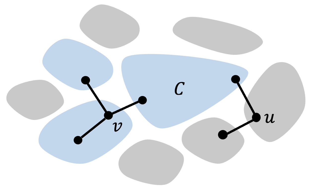
Figure 1: Illustration of the CIP. The regions correspond to the clusters in a partition $\Pi$. Node $v$ satisfies $D_{\Pi}(v)=3$ since it intersects $3$ clusters (colored in blue). Nodes $u,v$ intersect a common cluster $C$, so $uv\in E_{\Pi}$.

We emphasize that each node has a “self-loop”, since each vertex interferes with itself. The reader should not confuse the above independence graph with the interference graph. (The former is, in fact, always a supergraph of the latter)

The independence graph has the following nice property that will be useful when analyzing the variance: If $vv^{\prime}\notin E_{\Pi}$, then $v,v^{\prime}$ do not intersect any common cluster, and hence their outcomes and exposure mappings are independent.

Lemma 2.8 (Independence for Far-apart Agents).

Fix a partition $\Pi$ and $r\geq 0$. Suppose $v,v^{\prime}\in V$ and $vv^{\prime}\notin E_{\Pi}$. Then, for any $t,t^{\prime}\in[T]$, we have $\widehat{\Delta}^{r}_{vt}\perp\widehat{\Delta}_{v^{\prime}t^{\prime}}^{r}$.

To see this, recall that for each time block $B\subseteq[T]$ and cluster $C\subseteq V$, all units in the cylinder $B\times C$ are assigned the same treatment $A_{CB}$. Under this notation, $X_{vta}^{r}$ and $Y_{vt}$ only depend on the set of random variables $\{A_{CB}:(C,B)\in{\cal C}_{v}\}$ where ${\cal C}_{v}$ is the collection of cylinders that intersect ${\cal N}(v)\times[t-r,t]$, formally given by

$${\cal C}_{v}:=\left\{(C,B):\ C\cap{\cal N}(v)\neq\emptyset\ \text{ and }\ B\cap[t-r,t]\neq\emptyset\right\}.$$

Moreover, note that ${\cal C}_{v}\cap{\cal C}_{v^{\prime}}=\emptyset$ if $vv^{\prime}\notin E_{\Pi}$. Lemma 2.8 then follows since $(A_{CB})$ are independent for each cylinder. Finally, we define the combinatorial interference parameters (CIP) $\bar{d}_{\Pi}$ and $\zeta_{\Pi}$ which play a key role in our results.

Definition 2.9 (Combinatorial Interference Parameters).

Let $\Pi$ be a partition of $V$. Define $\bar{d}_{\Pi}=\frac{1}{N}\sum_{v\in V}d_{\Pi}(v)$ and

$$\zeta_{\Pi}=\zeta_{\Pi}(r,\ell):=\frac{1}{N}\sum_{vv^{\prime}\in E_{\Pi}}2^{(1+\lceil\frac{r}{\ell}\rceil)(D_{\Pi}(v)+D_{\Pi}(v^{\prime}))}.$$

Despite its intimidating appearance, the above term is quite natural. As we will see in Section 5, each unit $v$ intersects $(1+\lceil\frac{r}{\ell}\rceil)D_{\Pi}(v)$ cylinders, and hence its exposure probability is $2^{-(1+\lceil\frac{r}{\ell}\rceil)D_{\Pi}(v)}$. Thus, the covariance between the HT terms of $v,v^{\prime}$ is bounded by

$$2^{(1+\lceil\frac{r}{\ell}\rceil)D_{\Pi}(v)}\cdot 2^{(1+\lceil\frac{r}{\ell}\rceil)D_{\Pi}(v^{\prime})}=2^{(1+\lceil\frac{r}{\ell}\rceil)(D_{\Pi}(v)+D_{\Pi}(v^{\prime}))},$$

and $\zeta_{\Pi}$ arises naturally by summing all edges $vv^{\prime}\in E_{\Pi}$.

3 Main Results

We split the statement of our main result into two parts, by bounding the bias and variance, respectively.

Proposition 3.1 (Bias of the HT estimator).

For any $r\geq 0$, we have

$$|\mathbb{E}[\widehat{\Delta}^{r}]-\Delta|\leq 2e^{-r/t_{\rm mix}}.$$

To bound the variance, we need to consider the covariance between $\widehat{\Delta}_{vt}^{r}$ across $(v,t)$’s. As a key observation, given a partition of $V$ into clusters, the estimands at two nodes $u$, $v$ are dependent if and only if they intersect a common cluster. This motivates us to consider for each node $v$ the number of (i) clusters it intersects and (ii) nodes $v^{\prime}$ such that $v,v^{\prime}$ intersect a common cluster.

Proposition 3.2 (Variance of the HT estimator).

Let $\Pi$ be a partition of $V$. Then, for any $r,\ell\geq 0$, we have

$${\rm Var}(\widehat{\Delta}^{r})\lesssim\frac{(1+\sigma^{2})}{NT}\left(t_{\rm mix}e^{-\frac{\max\{\ell,r\}}{t_{\rm mix}}}\bar{d}_{\Pi}+\max\{r,\ell\}\zeta_{\Pi}\right).$$

The above may seem cumbersome because we have chosen to state the result for general $\bar{d}_{\Pi}$ and $\zeta_{\Pi}$. In Sections 3.1-3.4, we will show implications of our result specialized to natural classes of graphs for which $\zeta_{\Pi},\bar{d}_{\Pi}$ admit much simpler forms.

We prove Propositions 3.1 and 3.2 in Sections 4 and 5 respectively. Taken together, we deduce that for any fixed $\Pi$, by carefully choosing the block length $\ell$ (a parameter only of the design) and radius $r$ (a parameter only of the estimator) to trade off bias and variance, we can obtain $\sqrt{\log(NT)/(NT)}$-rate estimation for the original estimand $\Delta$.

Theorem 3.3 (MSE Upper Bound).

Suppose $\ell=r=t_{\rm mix}\log(NT)$, then

$${\rm MSE}(\widehat{\Delta}^{r})\lesssim\frac{(1+\sigma^{2})}{NT}\left(t_{\rm mix}e^{-\frac{\max\{\ell,r\}}{t_{\rm mix}}}\bar{d}_{\Pi}+\max\{r,\ell\}\zeta_{\Pi}\right).$$

Theorem 3.3 is asymptotically optimal in $T$ and $N$. Specifically, it is not hard to show that for any $N,T\geq 1$, there exists an instance without interference such that for any design and any estimator $\widehat{\Delta}$, we have ${\rm MSE}(\widehat{\Delta})=\Omega(1/NT)$. Note that this lower bound does not rule out adaptivity in the design, implying that the clustered switchback design is asymptotically optimal among all adaptive designs, despite its non-adaptivity.

In the following sections, we simplify $\zeta_{\Pi}$ and $\bar{d}_{\Pi}$ for specific classes of graphs and partitions, and deduce several corollaries of our main theorem.

3.1 No interference

We start with the simplest setting where the graph is a trivial graph where $E=\emptyset$. In other words, there is no interference between vertices.

Proposition 3.4 (CIP, No Interference).

Consider the trivial graph $G=(V,\emptyset)$ and let $\Pi$ be any partition of $V$. Then, $\bar{d}_{\Pi}=\frac{1}{N}\sum_{C\in\Pi}|C|^{2}$ and $\zeta_{\Pi}=\frac{2^{2(1+\lceil\frac{r}{\ell}\rceil)}}{2N}\sum_{C\in\Pi}|C|^{2}.$

We derive the first corollary by combining Proposition 3.4 with Theorem 3.3. Consider two trivial partitions: $\Pi_{\rm sgtn}$, where each cluster is singleton, and $\Pi_{\rm whole}$, where all vertices are in one cluster.

Corollary 3.5 (MSE with No Interference).

For $\Pi_{\rm sgtn}$, with $\ell=r=t_{\rm mix}\log(NT)$, we have ${\rm MSE}(\widehat{\Delta}^{r})\lesssim(1+\sigma^{2})t_{\rm mix}\cdot(NT)^{-1}\log(NT).$ Furthermore, for $\Pi_{\rm whole}$, with $\ell=r=t_{\rm mix}\log T$, we have

$${\rm MSE}(\widehat{\Delta}^{r})\lesssim(1+\sigma^{2})t_{\rm mix}T^{-1}\log T.$$

When $N=1$, our model and design coincide with the setup in Hu & Wager 2022. They focus on analyzing a class of difference-in-mean (DIM) estimators which compute the difference in average outcomes between blocks assigned to treatment vs control, ignoring data from time points that are too close to the boundary (referred to as the burn-in period). While they show that DIM estimators are limited to a MSE of $O(T^{-2/3})$, our results show that the truncated Horvitz-Thompson estimator obtains the optimal MSE rate, matching the improved rate of their concurrent bias-corrected estimator.

3.2 Bounded-degree Graphs

Now, we consider graphs with bounded degree. It is straightforward to show the following basic graph-theoretical result.

Proposition 3.6 (CIP for Bounded-degree Graphs).

Let $d$ be the maximum degree in $G$. Then, for the partition $\Pi=\Pi_{\rm sgtn}$, we have $\bar{d}_{\Pi}\leq d^{2}$ and $\zeta_{\Pi}(r,\ell)\leq d^{2}2^{2(1+\lceil\frac{r}{\ell}\rceil)d}.$

Substituting into Theorem 3.3, we have the following.

Corollary 3.7 (MSE on Bounded-degree Graphs).

Let $d$ be the maximum degree of $G$ and $\ell=r=t_{\rm mix}\log(NT)$, then

$${\rm MSE}(\widehat{\Delta}^{r})\lesssim(1+\sigma^{2})t_{\rm mix}d^{2}2^{4d}(NT)^{-1}\log(NT).$$

3.3 Restricted-Growth Graphs

The above bound has an unfavorable exponential dependence in $d$. This motivated Ugander et al. (2013) to introduce the following condition which assumes that the number of $h$-hop neighbors of each node is dominated by a geometric sequence. We denote by $d_{\rm hop}(\cdot,\cdot)$ the hop distance.

Definition 3.8 (Restricted Growth Condition).

Let $\kappa>0$ and consider a graph $G=(V,E)$. For any $r\geq 0$, define ${\cal N}_{r}(v)=\{u\in V:d_{\rm hop}(u,v)\leq r\}$. We say $G$ satisfies the $\kappa$-restricted growth condition (RGC), if for any $v\in V$,

$$|{\cal N}_{r+1}(v)|\leq\kappa\cdot|{\cal N}_{r}(v)|\quad\text{for all }r\geq 1.$$ (1)

To show their main result, Ugander et al. (2013) showed, via a greedy construction, that any graph admits a 3-net clustering. The RGC implies the following key property, stated as their Proposition 4.2 and rephrased as follows.

Proposition 3.9 (Bounding $D_{\Pi}$ with RGC).

Suppose that the interference graph satisfies the $\kappa$-RGC. Let $\Pi$ be any $3$-net clustering. Then, $D_{\Pi}(v)\leq\kappa^{3}$ for all $v\in V$.

Using this result, they showed that the MSE of the HT estimator is linear in $d$ if we view $\kappa$ as a constant; see their Proposition 4.4. We emphasize that we do not require the inequality in (1) for $r=0$, since otherwise we have $d\leq\kappa$ and hence the above result is exponential in $d^{3}$.

To apply our Theorem 3.3, consider a graph with $\kappa$-RGC and a $3$-net clustering. By Proposition 3.9, for each node $v$, we have $D_{\Pi}(v)\leq\kappa^{3}$. Moreover, note that $vv^{\prime}\in E_{\Pi}$ implies $d_{\rm hop}(v,v^{\prime})\leq 6$, and therefore $d_{\Pi}(v)\leq d\kappa^{5}$. Combining with Theorem 3.3, we obtain the following.

Corollary 3.10 (MSE for Graphs with RGC).

Suppose $G$ satisfies the $\kappa$-RGC and has maximum degree $d$. Then, for any $3$-net clustering $\Pi$, with $r=\ell=t_{\rm mix}\log(NT)$, we have

$${\rm MSE}(\widehat{\Delta}^{r})\lesssim(1+\sigma^{2})t_{\rm mix}d\kappa^{5}2^{4\kappa^{3}}(NT)^{-1}\log(NT).$$

When $T=1$, this matches the main result in Ugander et al. 2013 (i.e., their Proposition 4.4).

The above result is stronger than Corollary 3.7 on many graphs. For example, consider the $d$-spider graph: A special node $v_{0}$ is attached to $d$ paths, each of length $n/d$. Then, the $h$-hop neighborhood of $v_{0}$ contains $hd$ nodes, so $\kappa\leq 2$. Moreover, note that $\bar{d}_{\Pi}=O(1)$, so $d$ is replaced with $O(1)$ in the bound in Corollary 3.10. Another example is a sparse network of dense subgraphs (“communities”), which is a common structure in the study of social networks.

3.4 Spatial Interference

Suppose that the vertices are embedded into a $\sqrt{N}\times\sqrt{N}$ lattice. We assume that the transitions and outcomes at a node $v$ can interfere with nodes within a hop distance $h$. In other words, we include an edge $(u,v)$ in the interference graph $G$ if $d_{\rm hop}(u,v)\leq h$.

We explain how to achieve an MSE of $\tilde{O}(h^{2}/NT)$. Consider the following natural spatial clustering. For any $s>0$, we denote by $\Pi_{s}$ the uniform partition of the $\sqrt{N}\times\sqrt{N}$ lattice into squared-shape clusters of size $s\times s$.

Proposition 3.11 (CIP for Spatial Interference).

For $\Pi=\Pi_{2h}$, we have $\bar{d}_{\Pi}\lesssim h^{2}$ and $\zeta_{\Pi}\lesssim h^{2}2^{O(\lceil\frac{r}{\ell}\rceil)}.$

We immediately obtain the following from Theorem 3.3.

Corollary 3.12 (MSE for Spatial Interference).

Suppose $\ell=r=t_{\rm mix}\log(NT)$. Then, with $s=2h$, we have

$${\rm MSE}(\widehat{\Delta}^{r})\lesssim(1+\sigma^{2})h^{2}t_{\rm mix}\cdot(NT)^{-1}\log(NT).$$

4 Bias analysis

For any event $\mathcal{F}_{\bf W}$-measurable event $A$, denote by $\mathbb{P}_{A}$, $\mathbb{E}_{A}$, $\mathrm{Var}_{A}$, and $\mathrm{Cov}_{A}$ probability, expectation, variance, and covariance conditioned on $A$.

Next, we show that 2.1 implies a bound on how the law of $Y_{vt}$ under $\mathbb{P}_{\bf w}$ can vary as we vary $\bf w$. In particular, when $A=\{{\bf w}\}$ is a singleton set, we use the subscript ${\bf w}$ instead of $\{{\bf w}\}$.

Lemma 4.1 (Decaying Intertemporal Interference).

Consider any $t,m\in[T]$ with $1\leq m<t\leq T$ and $v\in V$. Given ${\bf w},{\bf w^{\prime}}\in\{0,1\}^{N\times T}$ such that $w_{v^{\prime}t^{\prime}}=w^{\prime}_{v^{\prime}t^{\prime}}$ for any round $t^{\prime}\in[t-m,t]$ and vertex $v^{\prime}\in{\cal N}(v)$, we have

$$d_{\rm TV}\left(\mathbb{P}_{\bf w}[Y_{vt}\in\cdot],\ \mathbb{P}_{\bf w^{\prime}}[Y_{vt}\in\cdot]\right)\leq e^{-m/t_{\rm mix}}.$$

The conclusion is reminiscent of the decaying interference assumption in Leung 2022 (albeit on distributions rather than realizations), which inspires us to consider an HT estimator as considered therein. However, their analysis is not readily applicable to our Markovian setting since they assume that the potential outcomes are deterministic.

Based on Lemma 4.1, we can establish the following bound.

Lemma 4.2 (Per-unit Bias).

For any $a\in\{0,1\}$, $r>0$, $v\in V$ and $t\in[T]$, we have

$$|\mathbb{E}[\widehat{Y}_{vta}^{r}]-\mathbb{E}[Y_{vt}|{\bf W}=a\cdot{\bf 1}]|\leq e^{-r/t_{\rm mix}}.$$

Now we are prepared to prove Proposition 3.1.

Proof of Proposition 3.1. By Lemma 4.2, we have

$$\quad\left|\mathbb{E}\left[\widehat{\Delta}^{r}\right]-\Delta\right|$$

$$\leq\frac{1}{NT}\sum_{v,t}\left|\Delta_{vt}-\mathbb{E}\left[\widehat{\Delta}_{vt}^{r}\right]\right|$$

$$\leq\frac{1}{NT}\sum_{a\in\{0,1\}}\sum_{v,t}\left|\mathbb{E}\left[\widehat{Y}_{vta}^{r}\right]-\mathbb{E}\left[Y_{vt}\mid{\bf W}=a\cdot{\bf 1}\right]\right|$$

$$\leq 2e^{-r/t_{\rm mix}}.$$ ∎

5 Variance analysis

We start with a bound that holds for all pairs of units.

Lemma 5.1 (Covariance bound).

For any $r,\ell\geq 0$, $v,v^{\prime}\in V$ and $t,t^{\prime}\in[T]$, we have

$${\rm Cov}\left(\widehat{\Delta}_{vt}^{r},\widehat{\Delta}_{v^{\prime}t^{\prime}}^{r}\right)\leq 4(1+\sigma^{2})2^{(1+\lceil\frac{r}{\ell}\rceil)(D_{\Pi}(v)+D_{\Pi}(v^{\prime}))}.$$

The above bound alone is not sufficient for our analysis, as it does not take advantage of the rapid mixing property. The rest of this section is dedicated to showing that for any pair of units that are far apart in time, the covariance of their HT terms decays exponentially in their temporal distance.

5.1 Covariance of Outcomes

We first show that if the realization of one random variable has little impact on the (conditional) distribution of another random variable, then they have low covariance.

Lemma 5.2 (Low Interference in Conditional Distribution Implies Low Covariance).

Let $U,V$ be two random variables and $g,h$ be real-valued functions defined on their respective realization spaces. If for some $\delta>0$, we have

$$d_{\rm TV}(\mathbb{P}[U\in\cdot\mid V],\ \mathbb{P}[U\in\cdot])\leq\delta\quad V\text{-almost surely },$$

then,

$$\quad{\rm Cov}(g(U),h(V))\leq\delta\cdot\|h(V)\|_{1}\cdot\|g(U)\|_{\infty}.$$

Viewing $V,U$ as outcomes in different rounds, we use the above to bound the covariance in the outcomes in terms of their temporal distance.

Lemma 5.3 (Covariance of Outcomes).

For any $A\subseteq\{0,1\}^{N\times T}$, vertices $v,v^{\prime}\in V$ and rounds $t,t^{\prime}\in[T]$, we have

$${\rm Cov}_{A}(Y_{vt},Y_{v^{\prime}t^{\prime}})\leq e^{-{|t-t^{\prime}|/{t_{{\rm mix}}}}}.$$

5.2 Covariance of HT terms

So far we have shown that the outcomes have low covariance if they are far apart in time. However, this does not immediately imply that the covariance between the HT terms $\widehat{\Delta}^{r}_{vt}$ is also low, since each HT term is a product of the outcome and the exposure mapping. To proceed, we need the following.

Lemma 5.4 (Bounding Covariance Using Conditional Covariance).

Let $U,V$ be independent Bernoulli random variables with means $p,q\in[0,1]$. Suppose $X,Y$ are random variables such that $X$ is independent of $V$ given $U$, and that $Y$ is independent of $U$ given $V$. Then,

$${\rm Cov}(UX,VY)=pq\cdot{\rm Cov}(X,Y\mid U=V=1).$$

We obtain the following bound by applying the above to the outcomes and exposure mappings in two rounds that are in different blocks and are further apart than $2r$ (in time).

Lemma 5.5 (Covariance of Far-apart HT terms).

Suppose $v,v^{\prime}\in V$ and $t,t^{\prime}\in[T]$ satisfy $\lceil t^{\prime}/\ell\rceil\neq\lceil t/\ell\rceil$ and $t^{\prime}+r<t-r$, then

$${\rm Cov}(\widehat{\Delta}_{vt}^{r},\widehat{\Delta}_{v^{\prime}t^{\prime}}^{r})\leq 4e^{-|t^{\prime}-t|/t_{\rm mix}}.$$

We remark that the restriction that $t,t^{\prime}$ are both farther than $2r$ apart in time and lie in distinct blocks are both necessary for the above exponential covariance bound. As an example, fix a vertex $v$ and consider $t,t^{\prime}\in[T]$ in the same block and suppose they are at a distance $r$ away from the boundary of this block. Then, the exposure mappings $X_{vta}^{r}$ and $X_{vt^{\prime}a}^{r}$ are the same, which we denote by $U$. Then,

$${\rm Cov}(UY_{v^{\prime}t^{\prime}}, UY_{vt})=p\cdot{\rm Cov}(Y_{v^{\prime}t^{\prime}},Y_{vt}\mid U=1)\ +$$

$$p(1-p)\cdot\mathbb{E}[Y_{v^{\prime}t^{\prime}}\mid U=1]\cdot\mathbb{E}[Y_{vt}\mid U=1]$$

where $p=\mathbb{P}[U=1]$. Therefore, we can choose the mean outcome function $\mu_{v^{\prime}t^{\prime}},\mu_{vt}$ to be large so that the above does not decrease exponentially in $|t^{\prime}-t|$.

5.3 Bounding the Variance: Proof of Proposition 3.2

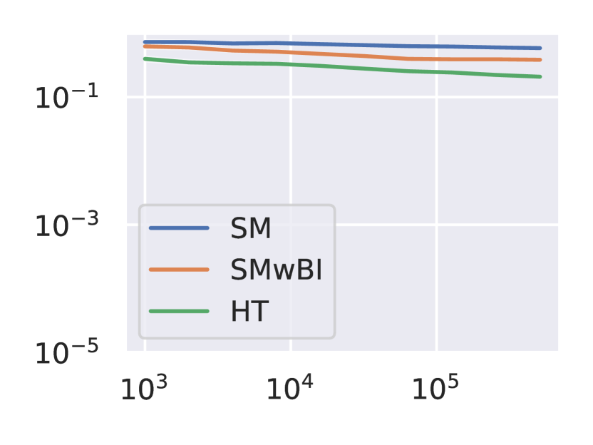
(a) $\lambda=5$

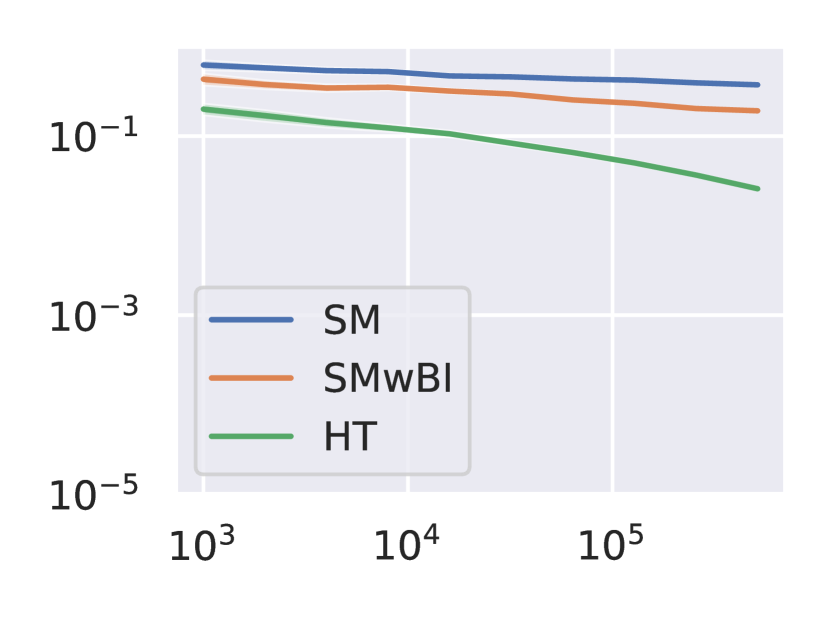
(b) $\lambda=10$

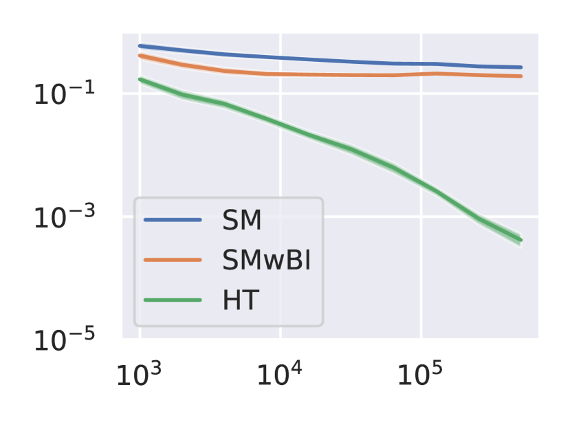
(c) $\lambda=15$

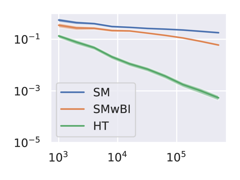
(d) $\lambda=20$

Figure 2: MSE of different estimators in the simulation study as $T$ and $\lambda$ vary

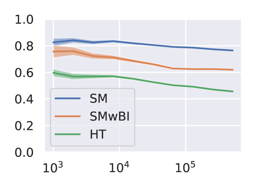
(e) $\lambda=5$

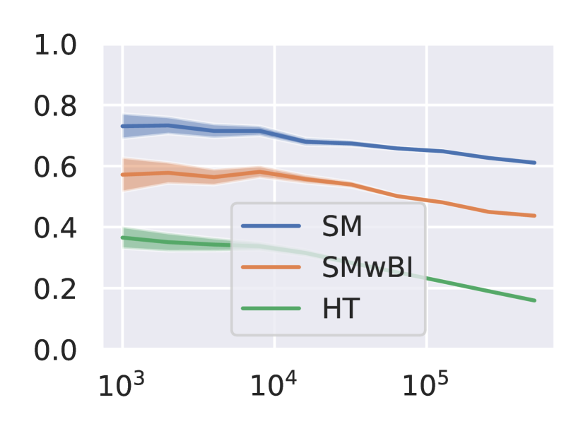
(f) $\lambda=10$

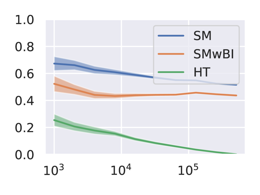
(g) $\lambda=15$

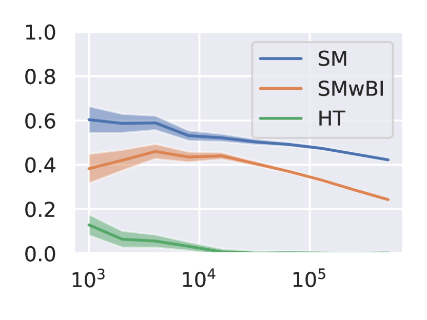
(h) $\lambda=20$

Figure 3: Bias of different estimators in the simulation study as $T$ and $\lambda$ vary

We are now ready to bound the variance. Write

$${\rm Var}\left(\widehat{\Delta}^{r}\right) ={\rm Var}\left(\frac{1}{NT}\sum_{(v,t)\in V\times[T]}\widehat{\Delta}_{vt}^{r}\right)$$

$$=\frac{1}{N^{2}T^{2}}\sum_{v,t}\sum_{v^{\prime},t^{\prime}}{\rm Cov}\left(\widehat{\Delta}_{v^{\prime}t^{\prime}},\widehat{\Delta}_{vt}\right).$$

By Lemma 2.8, if $vv^{\prime}\notin E_{\Pi}$, then ${\rm Cov}(\widehat{\Delta}_{v^{\prime}t^{\prime}},\widehat{\Delta}_{vt})=0$. Thus, for each $v$, we may consider only the vertices $v^{\prime}$ with $vv^{\prime}\in E_{\Pi}$ in the sum, and simplify the above as

$$\eqref{eqn:012523}=\frac{1}{N^{2}T^{2}}\sum_{(v,t)}\left(C_{vt}+F_{vt}\right)$$ (2)

where

$$C_{vt}:=\sum_{t^{\prime}:|t^{\prime}-t|\leq\max\{\ell,r\}}\sum_{v^{\prime}:vv^{\prime}\in E_{\Pi}}{\rm Cov}\left(\widehat{\Delta}_{vt}^{r},\widehat{\Delta}_{v^{\prime}t^{\prime}}^{r}\right)$$

and

$$F_{vt}:=\sum_{t^{\prime}:|t^{\prime}-t|\leq\max\{\ell,r\}}\sum_{v^{\prime}:vv^{\prime}\in E_{\Pi}}{\rm Cov}\left(\widehat{\Delta}_{vt}^{r},\widehat{\Delta}_{v^{\prime}t^{\prime}}^{r}\right).$$

Fix any $(v,t)\in V\times[T]$. By Lemma 5.1 and

$$C_{vt}\leq 4(1+\sigma^{2})\max\{\ell,r\}\alpha_{v},$$

and

$$\alpha_{v}:=\sum_{v^{\prime}:vv^{\prime}\in E_{\Pi}}2^{\left(1+\lceil\frac{r}{\ell}\rceil\right)\left(D_{\Pi}(v)+D_{\Pi}(v^{\prime})\right)}.$$

Summing over all $(v,t)$ and by the definition of $\zeta_{\Pi}$, we have

$$\sum_{v,t}C_{vt} \leq 4(1+\sigma^{2})\max\{\ell,r\}T\sum_{v\in V}\alpha_{v}$$

$$\leq 4(1+\sigma^{2})\max\{\ell,r\}T\cdot 2N\zeta_{\Pi}.$$ (3)

Next, we analyze $F_{vt}$. By Lemma 5.5, we have

$$F_{vt} =\sum_{v^{\prime}:vv^{\prime}\in E_{\Pi}}\sum_{t^{\prime}:|t^{\prime}-t|>\max\{\ell,r\}}{\rm Cov}\left(\widehat{\Delta}_{vt}^{r},\widehat{\Delta}_{v^{\prime}t^{\prime}}^{r}\right)$$

$$\leq\sum_{v^{\prime}:vv^{\prime}\in E_{\Pi}}2\int_{\max\{\ell,r\}}^{\infty}4e^{-z/t_{\rm mix}}\ dz$$

$$=8t_{\rm mix}e^{-\max\{\ell,r\}/t_{\rm mix}}\cdot d_{\Pi}(v),$$ (4)

where the “2” in the inequality arises since $s$ may be either greater or smaller than $t$. Combining Sections 5.3 and 5.3, we conclude that

$$\quad\ {\rm Var}\left(\widehat{\Delta}^{r}\right)$$

$$\leq\frac{1}{N^{2}T^{2}}\left(\sum_{v,t}C_{vt}+\sum_{v,t}F_{vt}\right)$$

$$\leq\frac{8(1+\sigma^{2})NT\zeta_{\Pi}+8Tt_{\rm mix}e^{-\frac{\max\{\ell,r\}}{t_{\rm mix}}}\sum_{v\in V}d_{\Pi}(v)}{N^{2}T^{2}}$$

$$=\frac{8}{NT}\left((1+\sigma^{2})\zeta_{\Pi}+t_{\rm mix}e^{-\frac{\max\{\ell,r\}}{t_{\rm mix}}}\bar{d}_{\Pi}\right).$$ ∎

6 Simulation study

We now turn to a simulation study of the performance of our method. We focus on the case of $N=1$ and a “pure” switchback design as a simple demonstration. We consider a state space $\mathcal{S}=\{-100,-99,\dots,100\}$ of size $201$ where, applying treatment $w\in\{0,1\}$ in a state $s\in\mathcal{S}$, we transit to $(s+1)\wedge 100$ with probability $\frac{18w+1}{20}$ and otherwise we transit to $(s-1)\vee-100$. We always start at $s_{0}=0$. We set $\mu_{t}(s,w)=\mathbb{I}[s>75]/2-\mathbb{I}[s<-75]/2+(\lceil(t-1)/l\rceil\;\mathrm{mod}\;2)-1/2$, where $l$ is the block length of the switchback design so as to create adversarial non-stationarity, and we set $\epsilon_{t}=0$. We vary $T\in\{1000,2000,4000,\dots,1024000\}$ and set the block length as $l=\lfloor\lambda\log T\rfloor$, where we vary $\lambda\in\{5,10,15,20\}$.

We evaluate three estimators, all on the same data from the same switchback design: our proposed radius-$r$-exposure-mapping HT estimator (HT) with $r=l$, a difference in sample means estimator (SM), and difference in sample means with “burn-in” (SMwBI) where we omit the first half of every block as suggested by Hu & Wager (2022). For each value of $T$ and $\lambda$, we run 200 replications of the simulation.

Figures 3 and 3 show the mean-squared error and bias, respectively, of each estimator as $T$ varies and for each value of $\lambda$, along with 95% confidence intervals over replications. We observe that setting $\lambda$ appropriately is important to ensure sufficient time to mix, and that overall the HT estimator outperforms differences in sample means, as predicted by our theory.

7 Conclusions

In the face of both spatial and temporal interference, we proposed an experimental design that combines two previously successful ideas: clustering and switchbacks. And, we demonstrated that such a design combined with a simple HT estimator achieves near-optimal estimation rates, both generalizing and improving results from the cross-sectional ($T=1$) and the single-unit ($N=1$) settings.

Our focus was, nonetheless, to demonstrate the potential, and there remain important avenues for future research. One is possible improvements to estimation. While nearly optimal in rate, HT can suffer high variance due to extreme weights. There may be opportunities to reduce variance such as by introducing control variates or using the weights as a clever covariate as in Scharfstein et al. (1999). Another avenue is possible improvements to the design. As the simulation study suggests, tuning the length of the blocks is important. Since mixing time may not be exactly known, it would be appealing to devise designs that can adapt to unknown mixing times.

Appendix A Proof of Proposition 3.4

Observe that for any $v,v^{\prime}\in V$, we have $vv^{\prime}\in E_{\Pi}$ if and only if $v,v^{\prime}$ lie in the same cluster. Thus,

$$\bar{d}_{\Pi}=\frac{1}{N}\sum_{C\in\Pi}\sum_{v\in C}d_{\Pi}(v)=\frac{1}{N}\sum_{C\in\Pi}|C|^{2}.$$

Now we consider $\zeta_{\Pi}$. For any $v\in V$, we have ${\cal N}(v)=\{v\}$. Therefore, the only cluster $v$ that intersects is the (unique) one that contains it, and hence $D_{\Pi}(v)=1$. It follows that

$$\zeta_{\Pi}(r,\ell) =\frac{1}{N}\sum_{vv^{\prime}\in E_{\Pi}}2^{2(1+\lceil\frac{r}{\ell}\rceil)}$$

$$\leq\frac{1}{N}\cdot 2^{2(1+\lceil\frac{r}{\ell}\rceil)}|E_{\Pi}|$$

$$\leq\frac{1}{2}2^{2(1+\lceil\frac{r}{\ell}\rceil)}\bar{d}_{\Pi}$$

$$\leq\frac{1}{2}2^{2(1+\lceil\frac{r}{\ell}\rceil)}\cdot\frac{1}{N}\sum_{C\in\Pi}|C|^{2},$$

where the second inequality follows is becuase $|E_{\Pi}|\leq\frac{1}{2}N\bar{d}_{\Pi}$. ∎

Appendix B Proof of Proposition 3.6

Denote by $\rm hop(\cdot,\cdot)$ the hop-distance in $G$. Observe that for any $v,v^{\prime}\in V$, we have $vv^{\prime}\in E_{\Pi}$ if and only if there exists a cluster $\{u\}$ that ${\cal N}(v),{\cal N}(v^{\prime})$ both intersect, which is equivalent to ${\rm hop}(v,v^{\prime})\leq 2$. Since every node has a maximum degree $d$, we deduce that every node is incident to $d^{2}$ edges in $G_{\Pi}$, and hence $\bar{d}_{\Pi}(v)\leq d^{2}.$

On the other hand, by definition we have $D_{\Pi}(v)\leq d$. Thus,

$$\zeta_{\Pi}(r,\ell)\leq\frac{1}{N}\sum_{vv^{\prime}\in E_{\Pi}}2^{(1+\lceil\frac{r}{\ell}\rceil)(d+d)}\leq\frac{1}{N}|E_{\Pi}|\cdot 2^{2(1+\lceil\frac{r}{\ell}\rceil)d}\leq d^{2}2^{2(1+\lceil\frac{r}{\ell}\rceil)d}.$$

where the last inequality follows since $|E_{\Pi}|=N\bar{d}_{\Pi}\leq Nd^{2}$. ∎

Appendix C Proof of Proposition 3.11

By basic geometry, we have $D_{\Pi}(v)\leq 4$ for each $v\in V$. To find $d_{\Pi}$, fix any $v\in V$ and consider a vertex $v^{\prime}$ with $vv^{\prime}\in E_{\Pi}$. Then, there exists $C\in\Pi$ such that ${\cal N}(v)\cap C$ and ${\cal N}(v^{\prime})\cap C,$ and hence $v^{\prime}$ lies in either $C$ or one of the 8 clusters neighboring $C$. Therefore, $d_{\Pi}(v)\leq 9s^{2}=36h^{2}.$ ∎

Appendix D Proof of Lemma 4.1

For any $s\in[T]$ and $j\in V$, we denote $f_{v^{\prime}t^{\prime}}=\mathbb{P}_{\bf w}[S_{v^{\prime}t^{\prime}}\in\cdot]$ and $f^{\prime}_{v^{\prime}t^{\prime}}=\mathbb{P}_{\bf w^{\prime}}[S_{v^{\prime}t^{\prime}}\in\cdot]$. Then, by the Chapman–Kolmogorov equation, we have

$$f_{j,s+1}=f_{v^{\prime}t^{\prime}}P^{w_{{\cal N}(u)},s}_{v^{\prime}t^{\prime}}\quad\text{and}\quad f^{\prime}_{j,s+1}=f^{\prime}_{v^{\prime}t^{\prime}}P^{w^{\prime}_{{\cal N}(u)},s}_{v^{\prime}t^{\prime}}.$$

Thus, if $t-m\leq s\leq t$, by 2.1 we have

$$d_{\rm TV}(f_{s+1},f^{\prime}_{s+1}) =d_{\rm TV}\left(f_{v^{\prime}t^{\prime}}P^{w_{{\cal N}(u)},s}_{v^{\prime}t^{\prime}},f^{\prime}_{v^{\prime}t^{\prime}}P^{w^{\prime}_{{\cal N}(u)},s}_{v^{\prime}t^{\prime}}\right)$$

$$=d_{\rm TV}\left(f_{v^{\prime}t^{\prime}}P^{w_{{\cal N}(u)},s}_{v^{\prime}t^{\prime}},f^{\prime}_{v^{\prime}t^{\prime}}P^{w_{{\cal N}(u)},s}_{v^{\prime}t^{\prime}}\right)$$

$$\leq e^{-1/t_{\rm mix}}\cdot d_{\rm TV}\left(f_{v^{\prime}t^{\prime}},f^{\prime}_{v^{\prime}t^{\prime}}\right),$$

where we used $w^{\prime}_{{\cal N}(u),s}=w_{{\cal N}(u),s}$ in the last equality. Applying the above for all $s=t-m,\dots,t$, we conclude that

$$d_{\rm TV}\left(\mathbb{P}_{\bf w}[Y_{vt}\in\cdot],\ \mathbb{P}_{\bf w^{\prime}}[Y_{vt}\in\cdot]\right)\leq d_{\rm TV}\left(f_{vt},f^{\prime}_{vt}\right)\leq e^{-m/t_{\rm mix}}\cdot d_{\rm TV}(f_{t-m},f^{\prime}_{t-m})\leq e^{-m/t_{\rm mix}},$$

where the first inequality is because $\mu_{vt}(\cdot,\cdot)\in[0,1]$, and the last inequality follows since the TV distance is at most $1$. ∎

Appendix E Proof of Lemma 4.2

For any $a\in\{0,1\}$, $v\in V$ and $t\in[T]$, we have

$$\mathbb{E}\left[\widehat{Y}_{vta}^{r}\right] =\mathbb{E}\left[\frac{X_{vta}^{r}}{p_{vta}^{r}}Y_{vt}\mid X_{vta}^{r}=1\right]\mathbb{P}\left[X_{vta}^{r}=1\right]+\mathbb{E}\left[\frac{X_{vta}^{r}}{p_{ta}^{r}}Y_{vt}\mid X_{vta}^{r}=0\right]\mathbb{P}\left[X_{vta}^{r}=0\right]$$

$$=\mathbb{E}\left[\frac{X_{t,a}^{r}}{p_{vta}^{r}}Y_{vt}\mid X_{vta}^{r}=1\right]p_{vta}^{r}+0$$

$$=\mathbb{E}\left[Y_{vt}\mid X_{vta}^{r}=1\right].$$

Note that $X_{vta}^{r}=1$ implies $w_{v^{\prime}t^{\prime}}=a$ for any $j\in{\cal N}(v)$ and $s\in[t-r,t]$. Therefore, by Lemma 4.1 with $m=r$, we have

$$d_{\rm TV}\left(\mathbb{P}_{\bf w}[Y_{vt}\in\cdot],\ \mathbb{P}_{a\cdot\bf 1}[Y_{vt}\in\cdot]\right)\leq e^{-r/t_{\rm mix}},$$

and hence

$$\left|\mathbb{E}\left[\widehat{Y}_{vta}^{r}\right]-\mathbb{E}\left[Y_{vt}\mid{\bf W}=a\cdot{\bf 1}\right]\right|=\left|\mathbb{E}\left[Y_{vt}\mid X_{vta}^{r}=1\right]-\mathbb{E}\left[Y_{vta}\mid{\bf W}=a\cdot{\bf 1}\right]\right|\leq e^{-r/t_{\rm mix}}.$$ ∎

Appendix F Proof of Lemma 5.1

Expanding the definition of $\widehat{\Delta}_{vt}^{r}$, we have

$${\rm Cov}\left(\widehat{\Delta}_{vt}^{r},\widehat{\Delta}_{v^{\prime}t^{\prime}}^{r}\right) ={\rm Cov}\left(\frac{X_{vt1}^{r}}{p_{vt1}^{r}}Y_{vt}-\frac{X_{vt0}^{r}}{p_{vt0}^{r}}Y_{vt},\ \frac{X_{vt1}^{r}}{p_{v^{\prime}t^{\prime}1}^{r}}Y_{v^{\prime}t^{\prime}}-\frac{X_{v^{\prime}t^{\prime}0}^{r}}{p_{v^{\prime}t^{\prime}0}^{r}}Y_{v^{\prime}t^{\prime}}\right)$$

$$\leq\sum_{a,a^{\prime}\in\{0,1\}}\left|{\rm Cov}\left(\frac{X_{vta}^{r}}{p_{vta}^{r}}Y_{vt},\ \frac{X_{v^{\prime}t^{\prime}a^{\prime}}^{r}}{p_{v^{\prime}t^{\prime}a^{\prime}}^{r}}Y_{v^{\prime}t^{\prime}}\right)\right|$$

$$\leq\sum_{a,a^{\prime}\in\{0,1\}}\frac{1}{p_{vta}^{r}}\frac{1}{p_{isa^{\prime}}^{r}}\left|{\rm Cov}\left(X_{vta}^{r}Y_{vt},\ X_{v^{\prime}t^{\prime}a^{\prime}}^{r}Y_{v^{\prime}t^{\prime}}\right)\right|$$

$$\leq\sum_{a,a^{\prime}\in\{0,1\}}\frac{1}{p_{vta}^{r}}\frac{1}{p_{v^{\prime}t^{\prime}a^{\prime}}^{r}}\sqrt{\mathbb{E}[(X_{vta}^{r}Y_{vt})^{2}]}\sqrt{\mathbb{E}[(X_{v^{\prime}t^{\prime}a^{\prime}}^{r}Y_{v^{\prime}t^{\prime}})^{2}]}$$

$$\leq\left(\frac{1}{p_{vt0}^{r}}+\frac{1}{p_{vt1}^{r}}\right)\left(\frac{1}{p_{v^{\prime}t^{\prime}0}^{r}}+\frac{1}{p_{v^{\prime}t^{\prime}1}^{r}}\right)(1+\sigma^{2}),$$ (5)

where the penultimate inequality is by Cauchy-Schwarz. Note that when $r\geq\ell$, the interval $[t-r,t]$ may intersect at most $\lceil r/\ell\rceil+1$ blocks. Thus, for any $a\in\{0,1\}$ we have

$$p_{vta}^{r}\geq 2^{-\left(1+\lceil\frac{r}{\ell}\rceil\right)(D_{\Pi}(v)+1)}.$$

On the other hand, when $0<r<\ell$, the interval $[t-r,t]$ can intersect at most two blocks, and hence

$$p_{ta}^{r}\geq\left(2^{D_{\Pi}(v)+1}\right)^{2}=2^{-(1+\lceil\frac{r}{\ell}\rceil)(D_{\Pi}(v)+1)}.$$

Therefore,

$$\eqref{eqn:121723}\leq(1+\sigma^{2})\left(2\cdot 2^{\left(1+\lceil\frac{r}{\ell}\rceil\right)\left(D_{\Pi}(v)+D_{\Pi}(v^{\prime})\right)}\right)^{2}=16(1+\sigma^{2})\cdot 2^{\left(1+\lceil\frac{r}{\ell}\rceil\right)\left(D_{\Pi}(v)+D_{\Pi}(v^{\prime})\right)}.$$ ∎

Appendix G Proof of Lemma 5.2

Denote by $\mu_{U,V},\mu_{U},\mu_{V},\mu_{U\mid V=v}$ the probability measures of $(U,V)$, $U$, $V$, and $U$ conditioned on $V=v$, respectively. We then have

$$|{\rm Cov}(g(U),h(V))| =|\mathbb{E}\left[g(U)h(V)\right]-\mathbb{E}[g(U)]\mathbb{E}[h(V)]|$$

$$=\left|\int_{v}h(v)\left(\int_{u}g(u)\left(\mu_{U\mid V=v}(du)-\mu_{U}(du)\right)\right)\mu_{V}(dv)\right|$$

$$\leq\int_{v}|h(v)|\cdot\|g(U)\|_{\infty}\cdot d_{\rm TV}(\mathbb{P}(U\in\cdot\mid V=v),\mathbb{P}(U\in\cdot))\mu_{V}(dv)$$

$$\leq\|h(V)\|_{1}\cdot\|g(U)\|_{\infty}\cdot\delta.$$ ∎

Appendix H Proof of Lemma 5.3

Wlog assume $t^{\prime}<t$. Then,

$${\rm Cov}_{A}(Y_{v^{\prime}t^{\prime}},Y_{vt}) ={\rm Cov}_{A}(\mu_{v^{\prime}t^{\prime}}(S_{v^{\prime}t^{\prime}},W_{v^{\prime}t^{\prime}}),\mu_{vt}(S_{vt},W_{vt}))+{\rm Cov}_{A}(\mu_{v^{\prime}t^{\prime}}(S_{v^{\prime}t^{\prime}},W_{v^{\prime}t^{\prime}}),\epsilon_{t})$$

$$\quad+{\rm Cov}_{A}(\epsilon_{v^{\prime}t^{\prime}},\mu_{vt}(S_{vt},W_{vt}))+{\rm Cov}_{A}(\epsilon_{v^{\prime}t^{\prime}},\epsilon_{vt}).$$

The latter three terms are zero by the exogenous noise assumption (in terms of covariances). By Lemma 4.1 and triangle inequality for $d_{\rm TV}$, for any $x\in\mathcal{S}$, we have

$$\quad d_{\rm TV}\left(\mathbb{P}_{A}\left[(S_{vt},W_{{\cal N}(v),t})\in\cdot\right],\ \mathbb{P}_{A}\left[(S_{vt},W_{{\cal N}(v),t})\in\cdot\mid S_{v^{\prime}t^{\prime}}=x,W_{{\cal N}(u),s}=w\right]\right)$$

$$=d_{\rm TV}\left(\mathbb{P}_{A}\left[S_{vt}\in\cdot\right],\ \mathbb{P}_{A}\left[S_{vt}\in\cdot\mid S_{v^{\prime}t^{\prime}}=x,W_{{\cal N}(u),s}=w\right]\right)$$

$$\leq e^{-{(t-t^{\prime})/{t_{{\rm mix}}}}}\cdot d_{\rm TV}(\mathbb{P}_{A}[S_{v^{\prime}t^{\prime}}\in\cdot],{\bf e}_{x})$$

$$\leq e^{-{(t-t^{\prime})/{t_{{\rm mix}}}}},$$ (6)

where ${\bf e}_{x}$ denotes the Dirac distribution at $x$, and the last inequality follows since the TV distance between any two distributions is at most $1$. Now apply Lemma 5.2 with $(S_{v^{\prime}t^{\prime}},W_{v^{\prime}t^{\prime}})$ in the role of $V$, with $(S_{vt},W_{vt})$ in the role of $U$, with $\mu_{vt}$ in the role of $g$, with $\mu_{v^{\prime}t^{\prime}}$ in the role of $h$, and with $e^{-(t-t^{\prime})/t_{\rm mix}}$ in the role of $\delta$. Noting that $\|g\|_{\infty},\|h\|_{\infty}\leq 1$ and combining with Appendix H, we conclude the statement. ∎

Appendix I Proof of Lemma 5.4

Since $U,V$ are Bernoulli, we have

$${\rm Cov}(UX,VY) =\mathbb{E}[UXVY]-\mathbb{E}[UX]\mathbb{E}[VY]$$

$$=\mathbb{E}[UXVY\mid U=V=1]pq-\mathbb{E}[UX\mid U=1]p\mathbb{E}[VY\mid V=1]q$$

$$=pq\left(\mathbb{E}[XY\mid U=V=1]-\mathbb{E}[X\mid U=1]\mathbb{E}[Y\mid V=1]\right).$$ (7)

Note that $X\perp V$ and $Y\perp U$, so

$$\mathbb{E}[X\mid U=1]=\mathbb{E}[X\mid U=V=1]\quad\text{and}\quad\mathbb{E}[Y\mid V=1]=\mathbb{E}[Y\mid U=V=1],$$

and therefore Appendix I becomes $pq\cdot{\rm Cov}(X,Y\mid U=V=1)$. ∎

Appendix J Proof of Lemma 5.5

Observe that for any (possibly identical) $a,a^{\prime}\in\{0,1\}$, since $t,t^{\prime}$ lie in distinct blocks and are more than $2r$ apart, we see that $X_{vta^{\prime}}^{r}$ and $X_{v^{\prime}t^{\prime}a}^{r}$ are independent. Thus, by Lemma 5.4, we have

$$\left|{\rm Cov}\left(\frac{X_{v^{\prime}t^{\prime}a}^{r}}{p_{v^{\prime}t^{\prime}a}^{r}}Y_{v^{\prime}t^{\prime}},\ \frac{X_{vta^{\prime}}^{r}}{p_{vta^{\prime}}^{r}}Y_{vt}\right)\right| =\frac{1}{p_{vta^{\prime}}^{r}}\frac{1}{p_{v^{\prime}t^{\prime}a}^{r}}\left|{\rm Cov}\left(X_{v^{\prime}t^{\prime}a}^{r}Y_{v^{\prime}t^{\prime}},\ X_{vta^{\prime}}^{r}Y_{vt}\right)\right|$$

$$=\left|{\rm Cov}\left(Y_{v^{\prime}t^{\prime}},Y_{vt}\mid X_{v^{\prime}t^{\prime}a}^{r}=X_{vta^{\prime}}^{r}=1\right)\right|.$$ (8)

To bound the above, consider the event

$$A=\{{\bf w}\in\{0,1\}^{N\times T}:X_{v^{\prime}t^{\prime}a}^{r}({\bf w})=X_{vta^{\prime}}^{r}({\bf w})=1\},$$

so that by Lemma 5.3 we have

$$\eqref{eqn:121423}=|{\rm Cov}_{A}(Y_{v^{\prime}t^{\prime}},Y_{vt})|\leq e^{-|t-t^{\prime}|/t_{\rm mix}}.$$

The conclusion follows by summing over all four combinations of $a,a^{\prime}\in\{0,1\}^{2}$. ∎

References

- Aronow et al. (2017) Aronow, P. M., Samii, C., et al. Estimating average causal effects under general interference, with application to a social network experiment. The Annals of Applied Statistics, 11(4):1912–1947, 2017.
- Basse & Airoldi (2018) Basse, G. W. and Airoldi, E. M. Model-assisted design of experiments in the presence of network-correlated outcomes. Biometrika, 105(4):849–858, 2018.
- Basse et al. (2019) Basse, G. W., Feller, A., and Toulis, P. Randomization tests of causal effects under interference. Biometrika, 106(2):487–494, 2019.
- Blake & Coey (2014) Blake, T. and Coey, D. Why marketplace experimentation is harder than it seems: The role of test-control interference. In Proceedings of the fifteenth ACM conference on Economics and computation, pp. 567–582, 2014.
- Bojinov et al. (2023) Bojinov, I., Simchi-Levi, D., and Zhao, J. Design and analysis of switchback experiments. Management Science, 69(7):3759–3777, 2023.
- Cai et al. (2015) Cai, J., De Janvry, A., and Sadoulet, E. Social networks and the decision to insure. American Economic Journal: Applied Economics, 7(2):81–108, 2015.
- Chin (2019) Chin, A. Regression adjustments for estimating the global treatment effect in experiments with interference. Journal of Causal Inference, 7(2), 2019.
- Eckles et al. (2017) Eckles, D., Karrer, B., and Ugander, J. Design and analysis of experiments in networks: Reducing bias from interference. Journal of Causal Inference, 5(1), 2017.
- Farias et al. (2022) Farias, V., Li, A., Peng, T., and Zheng, A. Markovian interference in experiments. Advances in Neural Information Processing Systems, 35:535–549, 2022.
- Forastiere et al. (2021) Forastiere, L., Airoldi, E. M., and Mealli, F. Identification and estimation of treatment and interference effects in observational studies on networks. Journal of the American Statistical Association, 116(534):901–918, 2021.
- Glynn et al. (2020) Glynn, P. W., Johari, R., and Rasouli, M. Adaptive experimental design with temporal interference: A maximum likelihood approach. Advances in Neural Information Processing Systems, 33:15054–15064, 2020.
- Gui et al. (2015) Gui, H., Xu, Y., Bhasin, A., and Han, J. Network a/b testing: From sampling to estimation. In Proceedings of the 24th International Conference on World Wide Web, pp. 399–409. International World Wide Web Conferences Steering Committee, 2015.
- Horvitz & Thompson (1952) Horvitz, D. G. and Thompson, D. J. A generalization of sampling without replacement from a finite universe. Journal of the American statistical Association, 47(260):663–685, 1952.
- Hu & Wager (2022) Hu, Y. and Wager, S. Switchback experiments under geometric mixing. arXiv preprint arXiv:2209.00197, 2022.
- Jagadeesan et al. (2020) Jagadeesan, R., Pillai, N. S., and Volfovsky, A. Designs for estimating the treatment effect in networks with interference. 2020.
- Jiang & Li (2016) Jiang, N. and Li, L. Doubly robust off-policy value evaluation for reinforcement learning. In International Conference on Machine Learning, pp. 652–661. PMLR, 2016.
- Johari et al. (2022) Johari, R., Li, H., Liskovich, I., and Weintraub, G. Y. Experimental design in two-sided platforms: An analysis of bias. Management Science, 68(10):7069–7089, 2022.
- Kohavi & Thomke (2017) Kohavi, R. and Thomke, S. The surprising power of online experiments. Harvard business review, 95(5):74–82, 2017.
- Larsen et al. (2023) Larsen, N., Stallrich, J., Sengupta, S., Deng, A., Kohavi, R., and Stevens, N. T. Statistical challenges in online controlled experiments: A review of a/b testing methodology. The American Statistician, pp. 1–15, 2023.
- Leung (2022) Leung, M. P. Rate-optimal cluster-randomized designs for spatial interference. The Annals of Statistics, 50(5):3064–3087, 2022.
- Leung (2023) Leung, M. P. Network cluster-robust inference. Econometrica, 91(2):641–667, 2023.
- Li et al. (2021) Li, W., Sussman, D. L., and Kolaczyk, E. D. Causal inference under network interference with noise. arXiv preprint arXiv:2105.04518, 2021.
- Manski (2013) Manski, C. F. Identification of treatment response with social interactions. The Econometrics Journal, 16(1):S1–S23, 2013.
- Ni et al. (2023) Ni, T., Bojinov, I., and Zhao, J. Design of panel experiments with spatial and temporal interference. Available at SSRN 4466598, 2023.
- Sävje (2023) Sävje, F. Causal inference with misspecified exposure mappings: separating definitions and assumptions. Biometrika, pp. asad019, 2023.
- Scharfstein et al. (1999) Scharfstein, D. O., Rotnitzky, A., and Robins, J. M. Adjusting for nonignorable drop-out using semiparametric nonresponse models. Journal of the American Statistical Association, 94(448):1096–1120, 1999.
- Shi et al. (2023) Shi, C., Wang, X., Luo, S., Zhu, H., Ye, J., and Song, R. Dynamic causal effects evaluation in a/b testing with a reinforcement learning framework. Journal of the American Statistical Association, 118(543):2059–2071, 2023.
- Sussman & Airoldi (2017) Sussman, D. L. and Airoldi, E. M. Elements of estimation theory for causal effects in the presence of network interference. arXiv preprint arXiv:1702.03578, 2017.
- Thomas & Brunskill (2016) Thomas, P. and Brunskill, E. Data-efficient off-policy policy evaluation for reinforcement learning. In International Conference on Machine Learning, pp. 2139–2148. PMLR, 2016.
- Thomke (2020) Thomke, S. Building a culture of experimentation. Harvard Business Review, 98(2):40–47, 2020.
- Toulis & Kao (2013) Toulis, P. and Kao, E. Estimation of causal peer influence effects. In International conference on machine learning, pp. 1489–1497. PMLR, 2013.
- Ugander et al. (2013) Ugander, J., Karrer, B., Backstrom, L., and Kleinberg, J. Graph cluster randomization: Network exposure to multiple universes. In Proceedings of the 19th ACM SIGKDD international conference on Knowledge discovery and data mining, pp. 329–337, 2013.