Renormalization-Group Evolution for the Bottom-Meson Soft Function

Abstract

We determine for the first time the renormalization-group (RG) evolution equation for the $B$-meson soft function dictating the non-perturbative strong interaction dynamics of the long-distance penguin contributions to the exclusive $b\to q\ell^{+}\ell^{-}$ and $b\to q\gamma$ decays. The distinctive feature of the ultraviolet renormalization of this fundamental distribution amplitude consists in the novel pattern of mixing positive into negative support for an arbitrary initial condition. The exact solution to this integro-differential RG evolution equation of the bottom-meson soft function is then derived with the Laplace transform technique, allowing for the model-independent extraction of the desired asymptotic behaviour at large/small partonic momenta.

I Introduction

The light-cone distribution amplitudes (LCDAs) of the bottom-meson are the fundamental non-perturbative ingredients for the model-independent description of exclusive $B$-meson decays into energetic particles. These crucial hadronic quantities are in high demand for exploring factorization properties of a wide range of the non-hadronic $B$-meson decay form factors Korchemsky et al. (2000); Lunghi et al. (2003); Bosch et al. (2003); Beneke and Rohrwild (2011); Galda et al. (2022); Beneke et al. (2020); Shen et al. (2020); Wang et al. (2022), and of the semi-leptonic and non-leptonic heavy-hadron decay amplitudes Beneke and Feldmann (2001); Beneke and Yang (2006); Hill et al. (2004); Beneke et al. (1999, 2000); Lü et al. (2023) at leading power in $\Lambda_{\rm QCD}/m_{b}$. They also dictate the infrared dynamics of the appropriate $B$-meson-to-vacuum correlation functions suitable for constructing the desired light-cone sum rules of numerous bottom-meson decay matrix elements Khodjamirian et al. (2005, 2007); De Fazio et al. (2006, 2008); Li et al. (2009); Wang and Shen (2015); Lü et al. (2019); Cui et al. (2023a); Gao et al. (2020); Wang et al. (2017); Gao et al. (2022); Cui et al. (2023b); Braun and Khodjamirian (2013); Wang (2016); Wang and Shen (2018); Beneke et al. (2018); Khodjamirian et al. (2023). Consequently, it has become the top priority to deepen our understanding towards both the non-perturbative behaviours Braun et al. (2004); Khodjamirian et al. (2020); Rahimi and Wald (2021); Wang et al. (2020) and the perturbative features Lange and Neubert (2003); Bell et al. (2013); Braun and Manashov (2014); Braun et al. (2019); Lee and Neubert (2005); Feldmann et al. (2014); Galda and Neubert (2020); Liu and Neubert (2020); Feldmann et al. (2022, 2023); Kawamura and Tanaka (2009, 2010) of the $B$-meson LCDAs for the sake of pinning down the theory uncertainties of the exclusive $B$-meson decay observables, motivated by the ever-increasing precision of the experimental measurements at LHCb and Belle II.

Advancing the field-theoretical computations of the interesting $B$-meson decay observables in the perturbative factorization framework necessitates further the robust control of the subleading-power contributions in the heavy quark expansion. Unsurprisingly, the higher-twist bottom-meson LCDAs from the non-leading spin projections, from the transverse motion of quarks and anti-quarks in the leading-twist components, and from the non-minimal Fock states with additional partonic fields, defined by the subleading light-cone matrix elements in heavy quark effective theory (HQET) Kawamura et al. (2001); Braun et al. (2015, 2017, 2018); Descotes-Genon and Offen (2009); Knodlseder and Offen (2011); Braun (2022), will appear in the theory description of the power-suppressed corrections with the QCD-based methods Beneke and Feldmann (2004); Khodjamirian et al. (2010, 2013); Gubernari et al. (2021); Piscopo and Rusov (2023). However, the intricate soft and collinear strong interaction fluctuations in the subleading-power contributions to the exclusive $B$-meson decay amplitudes are not necessarily captured by the non-local matrix elements of the composite operators with quark-gluon fields localized on the same light-cone direction Kozachuk and Melikhov (2018); Melikhov (2019, 2022, 2023); Belov et al. (2023); Qin et al. (2023) (see Benzke et al. (2010) for discussions on the inclusive $\bar{B}\to X_{s}\gamma$ decay). An excellent manifestation of the complex infrared structure for the exclusive heavy-hadron decay amplitude at next-to-leading power can be understood from the soft-collinear factorization formula of the long-distance penguin contribution to the double radiative $\bar{B}_{d,s}\to\gamma\gamma$ decays, which demands an introduction of the generalized three-particle distribution amplitude $\Phi_{\rm G}(\omega_{1},\omega_{2},\mu)$ defined by the soft matrix element with non-aligned fields Qin et al. (2023). Importantly, this new type of subleading $B$-meson soft functions will be also indispensable for QCD calculations of the charm-loop effects in the flagship electroweak penguin decay channels at the LHCb experiment. Extending the generalized HQET distribution amplitudes to investigations of the subleading-power corrections in the semileptonic $\Lambda_{b}\to\Lambda\ell^{+}\ell^{-}$ decays at large hadronic recoil Wang et al. (2009a); Aslam et al. (2008); Wang et al. (2009b); Mannel and Wang (2011); Feldmann and Yip (2012); Wang (2012); Böer et al. (2015); Wang and Shen (2016, 2016) can be further anticipated (see for instance Feldmann and Gubernari (2023)) under the influence of the improved LHCb measurements on the branching fraction and angular observables Aaij et al. (2015).

Apparently, the eventual factorization formulae of the long-distance penguin contributions to the exclusive $b\to q\ell^{+}\ell^{-}$ and $b\to q\gamma$ decays cannot be established without controlling the renormalization-scale dependence of such generalized $B$-meson distribution amplitudes. It is the primary objective of this Letter to derive the renormalization-group (RG) evolution equation of the soft function $\Phi_{\rm G}(\omega_{1},\omega_{2},\mu)$ and to present subsequently its exact analytic solution with the Laplace transform technique. We will then report on a novel observation of the dynamical properties of this generalized distribution amplitude, in striking contrast to the three-particle $B$-meson LCDAs Braun et al. (2017), which can be attributed to the soft-gluon interaction between the two Wilson lines in distinct light-cone directions. Phenomenological implications of the evolution effect due to the one-loop anomalous dimension will be further discussed with one sample model for the generalized bottom-meson distribution amplitude.

II The RG evolution equation

The generalized bottom-meson distribution amplitude $\Phi_{\rm G}$ entering the factorization formula for the soft-gluon radiative corrections to $\bar{B}_{q}\to\gamma\gamma$ is defined by the non-local HQET matrix element Qin et al. (2023)

$$\langle 0|(\bar{q}_{s}S_{n})(\tau_{1}n)\,(S_{n}^{\dagger}\,S_{\bar{n}})(0)\,(S_{\bar{n}}^{\dagger}\,g_{s}\,G_{\mu\nu}\,S_{\bar{n}})(\tau_{2}\bar{n})\,\,\bar{n}^{\nu}\not\!n\gamma_{\perp}^{\mu}\gamma_{5}\,(S_{\bar{n}}^{\dagger}h_{v})(0)|\bar{B}_{v}\rangle$$

$$=2\,{\cal F}_{B}(\mu)\,m_{B}\,\int_{-\infty}^{+\infty}d\omega_{1}\,\int_{-\infty}^{+\infty}d\omega_{2}\,{\rm exp}\left[-i(\omega_{1}\tau_{1}+\omega_{2}\tau_{2})\right]\,\Phi_{\rm G}(\omega_{1},\omega_{2},\mu)\,,$$ (1)

where the soft Wilson lines $S_{n}$ and $S_{\bar{n}}$ along the distinct light-cone directions of $n$ and $\bar{n}$ are introduced to maintain gauge invariance. To determine the RG equation of $\Phi_{\rm G}$, we first express the renormalized operator ${\cal O}_{\rm G}^{\rm ren}$ in terms of the corresponding bare operator

$${\cal O}_{\rm G}^{\rm ren}(\omega_{1},\omega_{2},\mu) = \int_{-\infty}^{+\infty}d\omega_{1}^{\prime}\int_{-\infty}^{+\infty}d\omega_{2}^{\prime}Z_{\rm G}(\omega_{1},\omega_{2},\omega_{1}^{\prime},\omega_{2}^{\prime},\mu)$$ (2)

$$\times\,{\cal O}_{\rm G}^{\rm bare}(\omega_{1}^{\prime},\omega_{2}^{\prime})\,,$$

where ${\cal O}_{\rm G}$ stands for the two-dimensional Fourier transform of the non-local operator on the left-hand side of (1). The convolutions in $\omega_{1,2}^{\prime}$ arise from the fact that the composite operators with different momentum variables $\omega_{1,2}$ can mix into each other under the ultraviolet (UV) renormalization. The renormalization constant $Z_{G}$ calculable in perturbation theory enables us to derive the anomalous dimension in the RG evolution equation

$${d\over d\ln\mu}\Phi_{\rm G}(\omega_{1},\omega_{2},\mu) = -\int_{-\infty}^{+\infty}d\omega_{1}^{\prime}\int_{-\infty}^{+\infty}d\omega_{2}^{\prime}\,\Phi_{\rm G}(\omega_{1}^{\prime},\omega_{2}^{\prime},\mu)$$ (3)

$$\times\,\Gamma_{\rm G}(\omega_{1},\omega_{2},\omega_{1}^{\prime},\omega_{2}^{\prime},\mu)\,,$$

by virtue of the customary relation

$$\Gamma_{\rm G} = \int_{-\infty}^{+\infty}\,d\omega_{1}^{\prime\prime}\,\int_{-\infty}^{+\infty}d\omega_{2}^{\prime\prime}\,Z_{\rm G}(\omega_{1},\omega_{2},\omega_{1}^{\prime\prime},\omega_{2}^{\prime\prime},\mu)$$ (4)

$$\hskip 73.97733pt\times\,{dZ_{\rm G}^{-1}(\omega_{1}^{\prime\prime},\omega_{2}^{\prime\prime},\omega_{1}^{\prime},\omega_{2}^{\prime},\mu)\over d\ln\mu}$$

$$+\,\delta(\omega_{1}-\omega_{1}^{\prime})\,\delta(\omega_{2}-\omega_{2}^{\prime})\,{d\ln{\cal F}_{B}(\mu)\over d\ln\mu}.$$

The renormalization-scale dependence of ${\cal F}_{B}(\mu)$ has been determined at four loops Grozin (2023). The renormalization constant $Z_{\rm G}$ can be obtained by evaluating the matrix element of ${\cal O}_{\rm G}(\omega_{1},\omega_{2})$ with the partonic external state $\langle 0|{\cal O}_{\rm G}(\omega_{1},\omega_{2})|\bar{q}(\omega_{1}^{\prime})g(\omega_{2}^{\prime},\eta)h_{v}\rangle$. The variables $\omega_{1}^{\prime}\equiv n\cdot k_{1}$ and $\omega_{2}^{\prime}\equiv\bar{n}\cdot k_{2}$ correspond to the particular light-cone components of the soft quark and gluon momenta, while $\eta$ represents the polarization vector of the external gluon.

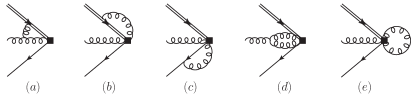
Figure 1: Sample Feynman diagrams for evaluating the one-loop QCD correction to the soft function $\Phi_{\rm G}$. The non-local vertices with two and three gluons include all possible combinations of the gluon emanating from the field strength tensor and from the soft Wilson lines $S_{n}$ and $S_{\bar{n}}$.

The sample Feynman diagrams for evaluating the renormalization factor $Z_{\rm G}$ at ${\cal O}(\alpha_{s})$ are explicitly displayed in Figure 1. We adopt dimensional regularization with space-time dimension $d=4-2\epsilon$ to extract the UV singularities and implement off-shell regularization to isolate the infrared (IR) divergences of the considered partonic matrix element. In analogy to the ${\cal O}(\alpha_{s})$ correction to $\phi_{B}^{+}(\omega,\mu)$ Grozin and Neubert (1997); Lange and Neubert (2003); Braun et al. (2004); Bell and Feldmann (2008), the soft-gluon exchange between the effective heavy quark and the light quark does not yield the UV-divergent contribution in Feynman gauge which is employed throughout our calculation. In addition, the one-gluon exchange between the light quark and the external gluon field is UV finite, on the basis of the power-counting analysis of the transverse-momentum $\ell_{\perp}$ integration. Moreover, connecting one soft gluon from $G_{\mu\nu}(\tau_{2}\bar{n})$ to the external bottom quark generates a vanishing correction, since the yielding integrand is an odd function of $\ell_{\perp}$. The one-particle irreducible diagram from attaching the single gluon field of $G_{\mu\nu}(\tau_{2}\bar{n})$ to the external light quark also brings about the UV finite effect, in terms of the power-counting analysis of the $\ell_{\perp}$ integral.

The most distinctive feature of $\Gamma_{\rm G}$ stems from the diagram (e) in Figure 1 comprising of four independent pieces: I) both two gluons in the loop from the soft Wilson lines while the external gluon from the field strength tensor; II) the two gluons in the loop from the Wilson lines along the $n$ direction and $G_{\mu\nu}(\tau_{2}\bar{n})$ while the external gluon again from the field strength tensor; III) the two gluons in the loop from the Wilson lines along the $n$ direction and $G_{\mu\nu}(\tau_{2}\bar{n})$ while the external gluon from the Wilson lines; IV) both two gluons in the loop from $G_{\mu\nu}(\tau_{2}\bar{n})$ while the external gluon from the soft Wilson lines. The third type of the ${\cal O}(\alpha_{s})$ correction vanishes, because the obtained integrand of the $\ell_{\perp}$ integral turns out to be an odd function. Contracting the two gluon fields from the non-Abelian term in the field strength tensor (namely, the fourth type mechanism) evidently generates a vanishing contribution. Moreover, the second class of the QCD correction is cancelled by the relevant contribution from the diagram (d). The remaining type-I correction from the diagram (e) can be cast in the form

$$Z_{\rm G}^{(\rm e)}\supset{\alpha_{s}\over 4\pi}\,{C_{A}\over\epsilon}\,\bigg{\{}\left[{1\over\epsilon}+\ln{\mu^{2}\over\omega_{1}\omega_{2}-i0}+i\,\pi\,\theta(\omega_{1}\omega_{2})\right]$$

$$\hskip 71.13188pt\times\,\delta(\omega_{1}-\omega_{1}^{\prime})\,\delta(\omega_{2}-\omega_{2}^{\prime})+\left({i\over 2\,\pi}\right)\,$$ (5)

$$\left[H_{+}(\omega_{1},\omega_{1}^{\prime})-H_{-}(\omega_{1},\omega_{1}^{\prime})-2i\pi\delta(\omega_{1}-\omega_{1}^{\prime})\,\theta(\omega_{2}^{\prime}-\omega_{2})\right]$$

$$\left[H_{+}(\omega_{2},\omega_{2}^{\prime})-H_{-}(\omega_{2},\omega_{2}^{\prime})-2i\pi\delta(\omega_{2}-\omega_{2}^{\prime})\,\theta(\omega_{1}^{\prime}-\omega_{1})\right]\bigg{\}},$$

where we have introduced the two primitive kernels $H_{\pm}(\omega_{i},\omega_{i}^{\prime})=\theta(\pm\omega_{i})F^{>(<)}(\omega_{i},\omega_{i}^{\prime})+\theta(\mp\omega_{i})G^{<(>)}(\omega_{i},\omega_{i}^{\prime})$ as defined in Beneke et al. (2022) (see also Böer and Feldmann (2023) for an overview). The superscripts “$>$” and “$<$” characterize the positive and negative light-cone momentum $\omega_{i}$, respectively. The manifest expressions for $F^{>(<)}$ and $G^{>(<)}$ read

$$F^{>}(\omega_{i},\omega_{i}^{\prime}) = \left[\frac{\omega_{i}\,\theta(\omega_{i}^{\prime}-\omega_{i})}{\omega_{i}^{\prime}\,(\omega_{i}^{\prime}-\omega_{i})}\right]_{+}+\left[\frac{\theta(\omega_{i}-\omega_{i}^{\prime})}{\omega_{i}-\omega_{i}^{\prime}}\right]_{\oplus}\,,$$

$$F^{<}(\omega_{i},\omega_{i}^{\prime}) = \left[\frac{\omega_{i}\,\theta(\omega_{i}-\omega_{i}^{\prime})}{\omega_{i}^{\prime}\,(\omega_{i}-\omega_{i}^{\prime})}\right]_{+}+\left[\frac{\theta(\omega_{i}^{\prime}-\omega_{i})}{\omega_{i}^{\prime}-\omega_{i}}\right]_{\ominus}\,,$$ (6)

$$G^{>}(\omega_{i},\omega_{i}^{\prime}) = (\omega_{i}+\omega_{i}^{\prime})\,\left[\frac{\theta(\omega_{i}^{\prime}-\omega_{i})}{\omega_{i}^{\prime}\,(\omega_{i}^{\prime}-\omega_{i})}\right]_{+}-i\pi\delta(\omega_{i}-\omega_{i}^{\prime})\,,$$

$$G^{<}(\omega_{i},\omega_{i}^{\prime}) = (\omega_{i}+\omega_{i}^{\prime})\,\left[\frac{\theta(\omega_{i}-\omega_{i}^{\prime})}{\omega_{i}^{\prime}\,(\omega_{i}-\omega_{i}^{\prime})}\right]_{+}+i\pi\delta(\omega_{i}-\omega_{i}^{\prime})\,.$$

The standard definition of the “+” distribution in the variable $\omega_{i}^{\prime}$ Lange and Neubert (2003) has been employed. We further introduce the modified $``\oplus"$ and $``\ominus"$ distributions to regulate the integrals of the non-local terms $\theta(\omega_{i}-\omega_{i}^{\prime})/(\omega_{i}-\omega_{i}^{\prime})$ (with $\omega_{i}^{(\prime)}>0$) and $\theta(\omega_{i}^{\prime}-\omega_{i})/(\omega_{i}^{\prime}-\omega_{i})$ (with $\omega_{i}^{(\prime)}<0$) Beneke et al. (2022)

$$\int_{-\infty}^{+\infty}d\omega_{i}^{\prime}\,\left[f(\omega_{i},\omega_{i}^{\prime})\right]_{\oplus/\ominus}\,\varphi(\omega_{i}^{\prime})$$

$$=\int_{-\infty}^{+\infty}d\omega_{i}^{\prime}\,f(\omega_{i},\omega_{i}^{\prime})\left[\varphi(\omega_{i}^{\prime})-\theta(\pm\omega_{i}^{\prime})\,\varphi(\omega_{i})\right]\,.$$ (7)

The modified $``\oplus"$ distribution in $F^{>}(\omega_{i},\omega_{i}^{\prime})$ generates an interesting pattern of evolving the negative $\omega_{i}^{\prime}$ into the positive $\omega_{i}$, while the modified $``\ominus"$ distribution in $F^{<}(\omega_{i},\omega_{i}^{\prime})$ yields the novel mixing from $\omega_{i}^{\prime}>0$ to $\omega_{i}<0$ as already noticed in Beneke et al. (2022). Consequently, the support region of $\Phi_{\rm G}(\omega_{1},\omega_{2},\mu)$ must be extended to the entire real axes $-\infty<\omega_{1,2}<+\infty$.

The next-to-leading-order (NLO) contributions from the two diagrams (a) and (b) with $\omega_{1,2}^{\prime}>0$ can be extracted from the counterpart expressions for the twist-three bottom-meson LCDA $\Phi_{3}(\omega_{1},\omega_{2},\mu)$ Offen and Descotes-Genon (2009), by invoking the exchange symmetry of $n\leftrightarrow\bar{n}$ in the diagrammatic computations (only valid at ${\cal O}(\alpha_{s})$ accuracy). The intriguing UV divergences in the negative support region from these two diagrams are captured by the modified $``\oplus"$ functions and by the emerged $\theta(-\omega_{i})$ terms with the standard $``+"$ distributions. The UV divergent contributions of the diagram (c) arise from attaching the gluon field of the Wilson line in the $n$ direction to the external light quark (while the external gluon state from the field strength). The yielding UV divergences in the positive support region can be inferred from the corresponding result of the leading-twist $B$-meson LCDA Lange and Neubert (2003); Bell and Feldmann (2008). The one-loop renormalization constant from this diagram in the negative support region can be obtained by implementing the replacement rules $\omega_{1}\to-\omega_{1}$ and $\omega_{1}^{\prime}\to-\omega_{1}^{\prime}$ in the determined expression at $\omega_{1}>0$ and $\omega_{1}^{\prime}>0$.

Collecting all the individual pieces together, we can readily derive the one-loop anomalous dimension

$$\Gamma_{\rm G} = {\alpha_{s}\over\pi}\,\bigg{\{}\left[C_{F}\left(\ln{\mu\over\omega_{1}-i0}-{1\over 2}\right)+C_{A}\left(\ln{\mu\over\omega_{2}-i0}+{i\over 2}\pi\right)\right]\delta(\omega_{1}-\omega_{1}^{\prime})\delta(\omega_{2}-\omega_{2}^{\prime})-C_{F}H_{+}(\omega_{1},\omega_{1}^{\prime})\delta(\omega_{2}-\omega_{2}^{\prime})$$

$$-\,C_{A}H_{+}(\omega_{2},\omega_{2}^{\prime})\delta(\omega_{1}-\omega_{1}^{\prime})+C_{A}\left({\omega_{2}\over\omega_{2}^{\prime\,2}}\right)\left[\theta(\omega_{2})\theta(\omega_{2}^{\prime}-\omega_{2})-\theta(-\omega_{2})\theta(\omega_{2}-\omega_{2}^{\prime})\right]\delta(\omega_{1}-\omega_{1}^{\prime})+\Delta\Gamma_{\rm G}\bigg{\}},$$

$$\Delta\Gamma_{\rm G} = {i\over 4}{C_{A}\over\pi}\left[H_{+}(\omega_{1},\omega_{1}^{\prime})-H_{-}(\omega_{1},\omega_{1}^{\prime})-2i\pi\delta(\omega_{1}-\omega_{1}^{\prime})\right]\,\left[H_{+}(\omega_{2},\omega_{2}^{\prime})-H_{-}(\omega_{2},\omega_{2}^{\prime})-2i\pi\delta(\omega_{2}-\omega_{2}^{\prime})\right].$$ (8)

It is straightforward to verify that the peculiar terms in (8) with the colour factor $C_{F}$ for $\omega_{1}>0$ and $\omega_{1}^{\prime}>0$ (apart from an overall factor of $\delta(\omega_{2}-\omega_{2}^{\prime})$) recovers the well-known Lange-Neubert kernel of the twist-two $B$-meson LCDA Lange and Neubert (2003). We further note that the one-loop anomalous dimension (8) becomes complex due to the soft-parton rescattering, in analogy to the earlier observation on the QED-generalized bottom-meson soft functions Beneke et al. (2022). In contrast with the evolution kernel for $\Phi_{3}(\omega_{1},\omega_{2},\mu)$ Offen and Descotes-Genon (2009), the one-gluon exchange between the light quark and the external gluon field in the UV renormalization of $\Phi_{\rm G}$ cannot generate the structure $\delta(\omega_{1}+\omega_{2}-\omega_{1}^{\prime}-\omega_{2}^{\prime})$ due to the momentum conservation in the common light-cone direction. In addition, the emerged structure of (8) implies that the counterpart coordinate-space evolution kernel could be expressed in terms of the generator of special conformal transformations $K=v^{\mu}K_{\mu}$ Braun et al. (2019) potentially. An elegant construction of this evolution kernel with the conformal symmetry technique Braun et al. (2003); Braun and Manashov (2014); Braun et al. (2019) is an important topic on its own and we plan to investigate this interesting issue in our subsequent work.

III The analytic solution

We are now in a position to derive an exact solution to the RG evolution equation of the generalized $B$-meson soft function with the Laplace (or Mellin) transform technique Lee and Neubert (2005); Bell et al. (2013); Ball et al. (2008); Li et al. (2013, 2014). The resulting RG equation in Laplace space becomes local in the first two arguments and can then be solved analytically. It turns out to be more advantageous to divide the support of the soft function $\Phi_{\rm G}$ into four separate pieces

$$\Phi_{\rm G}(\omega_{1},\omega_{2},\mu) = \theta(\omega_{1})\,\theta(\omega_{2})\,\Phi^{>,\,>}_{\rm G}(\omega_{1},\omega_{2},\mu)$$ (9)

$$+\,\theta(\omega_{1})\,\theta(-\omega_{2})\,\Phi^{>,\,<}_{\rm G}(\omega_{1},\omega_{2},\mu)$$

$$+\,\theta(-\omega_{1})\,\theta(\omega_{2})\,\Phi^{<,\,>}_{\rm G}(\omega_{1},\omega_{2},\mu)$$

$$+\,\theta(-\omega_{1})\,\theta(-\omega_{2})\,\Phi^{<,\,<}_{\rm G}(\omega_{1},\omega_{2},\mu)\,.\hskip 22.76228pt$$

Implementing the Laplace transform for these new soft functions $\Phi^{>(<),\,>(<)}_{\rm G}$ with respect to the two variables $\ln(\mu/\omega_{1})$ and $\ln(\mu/\omega_{2})$ leads to

$$\tilde{\Phi}^{>(<),\,>(<)}_{\rm G}(\eta_{1},\eta_{2},\mu) \equiv \int_{0}^{\infty}\,{d\omega_{1}\over\omega_{1}}\,\int_{0}^{\infty}{d\omega_{2}\over\omega_{2}}\left({\mu\over\omega_{1}}\right)^{\eta_{1}}$$ (10)

$$\left({\mu\over\omega_{2}}\right)^{\eta_{2}}\,\Phi^{>(<),\,>(<)}_{\rm G}(\pm\omega_{1},\,\pm\omega_{2},\,\mu)\,,$$

where the upper and lower signs in front of $\omega_{1,\,2}$ correspond to the superscripts “$>$” and “$<$”, respectively. Subsequently, we obtain a coupled system of the first-order differential equations for $\tilde{\Phi}^{>(<),\,>(<)}_{\rm G}$ in Laplace space (with $-1<{\rm Re}(\eta_{1,2})<0$)

$$\left({d\over d\ln\mu}-\eta_{1}-\eta_{2}\right)\,{\bf\tilde{\Phi}}_{\rm G}(\eta_{1},\eta_{2},\mu)$$ (11)

$$=-{\alpha_{s}(\mu)\over\pi}\,\left[\tilde{\Gamma}_{\rm G}^{(0)}+\tilde{\Gamma}_{\rm G}^{(1)}+\left({i\over 4\pi}\right)\,\tilde{\Gamma}_{\rm G}^{(2)}\right]\,{\bf\tilde{\Phi}}_{\rm G}(\eta_{1},\eta_{2},\mu)\,,$$

where ${\bf\tilde{\Phi}}_{\rm G}$ stands for the column vector $(\tilde{\Phi}^{>,\,>}_{\rm G}\,,\tilde{\Phi}^{>,\,<}_{\rm G}\,,\tilde{\Phi}^{<,\,>}_{\rm G}\,,\tilde{\Phi}^{<,\,<}_{\rm G})^{\rm T}$. The evolution matrices $\tilde{\Gamma}_{\rm G}^{(i)}$ ($i=0,\,1,\,2$) are given by

$$\tilde{\Gamma}_{\rm G}^{(0)} = \left[C_{F}\,\left(\partial_{\eta_{1}}-{1\over 2}\right)+C_{A}\,\left(\partial_{\eta_{2}}+{1\over 1-\eta_{2}}+{i\over 2}\,\pi\right)\right]\,,$$

$$\tilde{\Gamma}_{\rm G}^{(1)} = C_{F}\,\tilde{\Gamma}_{\rm G}^{(+)}(\eta_{1})\otimes\mathbf{1}_{\rm 2\times 2}+C_{A}\,\mathbf{1}_{\rm 2\times 2}\otimes\tilde{\Gamma}_{\rm G}^{(+)}(\eta_{2})\,,$$

$$\tilde{\Gamma}_{\rm G}^{(2)} = C_{A}\,\tilde{\Gamma}_{\rm G}^{(+-)}(\eta_{1})\otimes\tilde{\Gamma}_{\rm G}^{(+-)}(\eta_{2})\,.$$ (12)

For brevity, we have introduced the following conventions

$$\tilde{\Gamma}_{\rm G}^{(+)}(\eta) = \left(\begin{array}[]{cc}H_{\eta}+H_{-\eta}&\Gamma(\eta)\,\Gamma(1-\eta)\\ 0&\,\,H_{-1-\eta}+H_{-\eta}\\ \end{array}\right),$$ (15)

$$\tilde{\Gamma}_{\rm G}^{(+-)}(\eta) = \left(\begin{array}[]{cc}H_{\eta}-H_{-1-\eta}+i\,\pi&\Gamma(\eta)\,\Gamma(1-\eta)\\ -\Gamma(\eta)\,\Gamma(1-\eta)&\,\,H_{-1-\eta}-H_{\eta}+i\,\pi\\ \end{array}\right),$$ (18)

where $H_{\eta}$ is the Harmonic number function. Both the diagonal and non-diagonal terms of the evolution kernel for $\tilde{\Phi}^{>,\,>}_{\rm G}$ ($\tilde{\Phi}^{<,\,<}_{\rm G}$) with the colour factor $C_{F}$ appear to be identical to the corresponding expressions for the QED-generalized distribution amplitude $\tilde{\Phi}_{>}$ ($\tilde{\Phi}_{<}$) Beneke et al. (2022).

Diagonalizing the one-loop anomalous dimension matrix Buras et al. (1992) leads to the general solution in Laplace space

$${\bf\tilde{\Phi}}_{\rm G}(\eta_{1},\eta_{2},\mu)={\rm exp}\left[V+2\,\gamma_{E}\,(a_{1}+a_{2})\right]\,\left({\mu\over\mu_{0}}\right)^{\eta_{1}+\eta_{2}}\,$$

$$\hat{U}^{-1}(\eta_{1},\eta_{2})\,\,{\rm diag}\left(1,\,1,\,1,\,e^{-i\pi a_{2}}\right)\,\,\hat{U}(\eta_{1}+a_{1},\eta_{2}+a_{2})$$

$$\times\,\frac{\Gamma(1-\eta_{1})\,\Gamma(1+\eta_{1}+a_{1})}{\Gamma(1+\eta_{1})\,\Gamma(1-\eta_{1}-a_{1})}\,\frac{\Gamma(2-\eta_{2})\,\Gamma(1+\eta_{2}+a_{2})}{\Gamma(1+\eta_{2})\,\Gamma(2-\eta_{2}-a_{2})}\,$$

$$\times\,{\bf\tilde{\Phi}}_{\rm G}(\eta_{1}+a_{1},\eta_{2}+a_{2},\mu_{0}),\hskip 108.12054pt$$ (19)

where we have introduced the evolution functions Bell et al. (2013); Lee and Neubert (2005)

$$V = -\int_{\mu_{0}}^{\mu}{d\mu^{\prime}\over\mu^{\prime}}\frac{\alpha_{s}(\mu^{\prime})}{\pi}$$ (20)

$$\times\,\bigg{[}C_{F}\left(\ln{\mu^{\prime}\over\mu_{0}}-{1\over 2}\right)+C_{A}\left(\ln{\mu^{\prime}\over\mu_{0}}+{i\over 2}\pi\right)\bigg{]},$$

$$a_{1} = -\int_{\mu_{0}}^{\mu}{d\mu^{\prime}\over\mu^{\prime}}\,\frac{\alpha_{s}(\mu^{\prime})}{\pi}\,C_{F}\,,\hskip 5.69046pta_{2}=-\int_{\mu_{0}}^{\mu}{d\mu^{\prime}\over\mu^{\prime}}\,\frac{\alpha_{s}(\mu^{\prime})}{\pi}\,C_{A}\,.$$

The transformation matrix $\hat{U}$ in the obtained solution (19) can be written as

$$\hat{U}(\eta_{1},\eta_{2})=\left(\begin{array}[]{cc}1&-e^{-i\pi\eta_{1}}\\ 1&-e^{i\pi\eta_{1}}\\ \end{array}\right)\otimes\left(\begin{array}[]{cc}1&-e^{-i\pi\eta_{2}}\\ 1&-e^{i\pi\eta_{2}}\\ \end{array}\right)\,.\hskip 14.22636pt$$ (25)

Carrying out the inverse Laplace transformation with respect to the two variables $\eta_{1}$ and $\eta_{2}$, we then derive the desired momentum-space solution to the RG equation (3)

$${\bf{\Phi}}_{\rm G}(\omega_{1},\omega_{2},\mu) = {\rm exp}\left[V+2\gamma_{E}(a_{1}+a_{2})\right]\int_{0}^{\infty}{d\omega_{1}^{\prime}\over\omega_{1}^{\prime}}\int_{0}^{\infty}{d\omega_{2}^{\prime}\over\omega_{2}^{\prime}}$$ (26)

$$\left({\mu_{0}\over\omega_{1}^{\prime}}\right)^{a_{1}}\left({\mu_{0}\over\omega_{2}^{\prime}}\right)^{a_{2}}\left[{\cal J}_{1}\otimes{\cal J}_{2}+\frac{1-e^{-i\pi a_{2}}}{4}\,{\cal K}_{1}\otimes{\cal K}_{2}\right]$$

$$\times\,{\bf\Phi}_{\rm G}(\omega_{1}^{\prime},\omega_{2}^{\prime},\mu_{0}),$$

where ${\bf\Phi}_{\rm G}$ represents the column vector with the elements defined by the four momentum-space soft functions with the particular arguments on the right-hand side of (10). The evolution matrices ${\cal J}_{i}$ and ${\cal K}_{i}$ (with $i=1,\,2$) can be expressed in terms of the familiar Meijer-${\rm G}$ functions and we do not present their lengthy expressions here.

IV Phenomenological implications

In order to explore the asymptotic behaviours of the bottom-meson soft function at small and large quark and gluon momenta, we will take the exponential model with only the positive domain for the initial condition

$$\Phi_{\rm G}^{\rm exp}(\omega_{1},\omega_{2},\mu_{0}) = \frac{\lambda_{E}^{2}+\lambda_{H}^{2}}{6}\,{\omega_{1}\,\omega_{2}^{2}\over\omega_{0}^{5}}\,{\rm exp}\left(-{\omega_{1}+\omega_{2}\over\omega_{0}}\right)\,$$ (27)

$$\times\,\theta(\omega_{1})\,\theta(\omega_{2})\,,$$

at $\mu_{0}=1.0\,{\rm GeV}$, motivated by the non-perturbative analysis of the HQET sum rules at leading order in $\alpha_{s}$ Qin et al. (2023). The hadronic quantities $\lambda_{E}^{2}$ and $\lambda_{H}^{2}$ are defined by the effective matrix elements of the chromoelectric and chromomagnetic operators Grozin and Neubert (1997); Braun et al. (2017). It remains important to remark that the model-independent constraints from the operator-product-expansion (OPE) computation of the regularized moments Lee and Neubert (2005); Feldmann et al. (2014); Beneke et al. (2023) can be further implemented for constructing the QCD improved model of this soft function. In accordance with the general solution (26) and the asymptotic expansion of the Meijer-${\rm G}$ functions, we can determine the scaling behaviour of the $B$-meson soft function in the endpoint region $\omega_{1,2}\to 0$

$$\Phi_{\rm G}^{\rm exp}(\omega_{1}\to 0,\omega_{2}\to 0,\mu)$$

$$=\frac{\lambda_{E}^{2}+\lambda_{H}^{2}}{6}\,{1\over\omega_{0}^{2}}\,{\rm exp}\left[V+2\,\gamma_{E}\,(a_{1}+a_{2})\right]\left({\mu_{0}\over\omega_{0}}\right)^{a_{1}+a_{2}}$$

$$\hskip 14.22636pt\frac{1-e^{-i\pi a_{2}}}{4\pi^{2}}\Gamma(1+a_{1})\Gamma(1+a_{2})+{\cal O}\left({\omega_{1}\over\omega_{0}},{\omega_{2}\over\omega_{0}}\right).\hskip 14.22636pt$$ (28)

Interestingly, this soft function acquires a constant value in the limit $\omega_{1,2}\to 0$, bearing a resemblance to the counterpart asymptotic behaviour of the QED-generalized LCDA $\Phi_{0-}(\omega,\mu)$ Beneke et al. (2022).

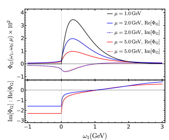
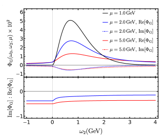
Figure 2: Theory predictions for the RG evolution of $\Phi_{\rm G}(\omega_{1},\omega_{0},\mu)$ (upper panel) and $\Phi_{\rm G}(\omega_{0},\omega_{2},\mu)$ (lower panel) by taking the exponential model (27) as an initial condition (black curves). The blue and red curves are obtained by evolving the soft functions to a hard-collinear scale $\mu=2.0\,{\rm GeV}$ and to a hard scale $\mu=5.0\,{\rm GeV}$, respectively. The ratios between the imaginary and real parts of the evolved soft functions are also shown explicitly. We have employed the numerical values of $\omega_{0}$, $\lambda_{E}^{2}$ and $\lambda_{H}^{2}$ from Shen et al. (2020).

Along the same vein, we can further derive the large-momentum behaviour of $\Phi_{\rm G}$ with the solution (26)

$$\Phi_{\rm G}^{\rm exp}(\omega_{1}\to\pm\infty,\omega_{2}\to\pm\infty,\mu)$$

$$\propto\frac{\lambda_{E}^{2}+\lambda_{H}^{2}}{6}\,{1\over\omega_{0}^{2}}\,{\rm exp}\left[V+2\,\gamma_{E}\,(a_{1}+a_{2})\right]\,\left({\mu_{0}\over\omega_{0}}\right)^{a_{1}+a_{2}}\,$$

$$\hskip 14.22636pt\left({\omega_{0}\over\pm\omega_{1}}\right)^{1+a_{1}}\,\left({\omega_{0}\over\pm\omega_{2}}\right)^{1+a_{2}}\,,$$ (29)

which turns out to be analogous to the well-known behaviour of the leading-twist $B$-meson LCDA Lange and Neubert (2003). We are then led to conclude that all non-negative moments of the soft function $\Phi_{\rm G}(\omega_{1},\omega_{2},\mu)$ are divergent. The non-existence of the normalization integral can also be understood from the logarithmic UV singularities of the HQET matrix element on the left-hand side of (1) at $\tau_{1,2}\to 0$ (see Braun et al. (2004) for the earlier discussion). Adopting the three-parameter ansätz for the bottom-meson soft function in Qin et al. (2023), we can further verify analytically that the determined scaling behaviours at $\omega_{1,2}\to 0$ and $\omega_{1,2}\to\pm\infty$ remain unchanged for this more general model.

To develop a transparent understanding of the RG evolution effect due to the one-loop anomalous dimension, we display in Figure 2 the numerical predictions for $\Phi_{\rm G}$ evolved to the two distinct renormalization scales $\mu=2.0\,{\rm GeV}$ and $5.0\,{\rm GeV}$. It is evident that incorporating the one-loop QCD evolution can bring about the considerable reduction of the soft function in the peak region at $\mu=2.0\,{\rm GeV}$ (as large as ${\cal O}(50\,\%)$ numerically). Moreover, the RG evolution can result in the positive correction in the large $\omega_{1,\,2}$ region due to the emergence of the radiative tail which falls off much slower than the initial behaviour (27). In particular, taking into account the leading-logarithmic (LL) evolution of the soft function $\Phi_{\rm G}$ can generate the noticeable imaginary part as anticipated: approximately ${\cal O}(20\,\%)$ of the corresponding real part, even if we start with the real-valued initial condition (27). This new strong-phase source will be of importance for predicting the CP-violating observables in the exclusive bottom-meson decays. The RG evolution effect from $\mu_{0}=1.0\,{\rm GeV}$ to $\mu=5.0\,{\rm GeV}$ becomes more pronounced than the observed pattern at $\mu=2.0\,{\rm GeV}$. The numerical features of the evolution effects in Figure 2 further indicate the constant phases of $\Phi_{\rm G}(\omega_{1},\omega_{0},\mu)$ and $\Phi_{\rm G}(\omega_{0},\omega_{2},\mu)$ in the negative domain, which remain true for an arbitrary real-valued initial condition factorizable in the two momentum variables with positive support.

V Conclusions

In conclusion, we have derived for the first time the RG evolution equation of the generalized $B$-meson distribution amplitude, defined by the subleading HQET matrix element with non-aligned partonic fields. The most striking feature of the UV renormalization kernel of the soft function consists in the novel pattern of mixing positive into negative support, irrespective of the initial behaviour of $\Phi_{\rm G}$, thus extending the support region of this generalized distribution amplitude to the entire real axes $-\infty<\omega_{1,2}<+\infty$. Adopting one sample model for the $B$-meson soft function, we have explicitly demonstrated that including the RG evolution from the hadronic scale $\mu_{0}=1.0\,{\rm GeV}$ to the hard-collinear scale $\mu=2.0\,{\rm GeV}$ can result in an enormous reduction of $\Phi_{\rm G}$ in the peak region. Extending our RG analysis to the generic soft functions defined with partonic fields localized on two distinct light-cone directions will be highly beneficial for evaluating the long-distance charming penguin contributions in the $B\to K^{(\ast)}\ell^{+}\ell^{-}$ and $B\to K^{\ast}\gamma$ decays.

References

- Korchemsky et al. (2000) G. P. Korchemsky, D. Pirjol, and T.-M. Yan, Phys. Rev. D 61, 114510 (2000), arXiv:hep-ph/9911427 .
- Lunghi et al. (2003) E. Lunghi, D. Pirjol, and D. Wyler, Nucl. Phys. B 649, 349 (2003), arXiv:hep-ph/0210091 .
- Bosch et al. (2003) S. W. Bosch, R. J. Hill, B. O. Lange, and M. Neubert, Phys. Rev. D 67, 094014 (2003), arXiv:hep-ph/0301123 .
- Beneke and Rohrwild (2011) M. Beneke and J. Rohrwild, Eur. Phys. J. C 71, 1818 (2011), arXiv:1110.3228 [hep-ph] .
- Galda et al. (2022) A. M. Galda, M. Neubert, and X. Wang, JHEP 07, 148 (2022), arXiv:2203.08202 [hep-ph] .
- Beneke et al. (2020) M. Beneke, C. Bobeth, and Y.-M. Wang, JHEP 12, 148 (2020), arXiv:2008.12494 [hep-ph] .
- Shen et al. (2020) Y.-L. Shen, Y.-M. Wang, and Y.-B. Wei, JHEP 12, 169 (2020), arXiv:2009.02723 [hep-ph] .
- Wang et al. (2022) C. Wang, Y.-M. Wang, and Y.-B. Wei, JHEP 02, 141 (2022), arXiv:2111.11811 [hep-ph] .
- Beneke and Feldmann (2001) M. Beneke and T. Feldmann, Nucl. Phys. B 592, 3 (2001), arXiv:hep-ph/0008255 .
- Beneke and Yang (2006) M. Beneke and D. Yang, Nucl. Phys. B 736, 34 (2006), arXiv:hep-ph/0508250 .
- Hill et al. (2004) R. J. Hill, T. Becher, S. J. Lee, and M. Neubert, JHEP 07, 081 (2004), arXiv:hep-ph/0404217 .
- Beneke et al. (1999) M. Beneke, G. Buchalla, M. Neubert, and C. T. Sachrajda, Phys. Rev. Lett. 83, 1914 (1999), arXiv:hep-ph/9905312 .
- Beneke et al. (2000) M. Beneke, G. Buchalla, M. Neubert, and C. T. Sachrajda, Nucl. Phys. B 591, 313 (2000), arXiv:hep-ph/0006124 .
- Lü et al. (2023) C.-D. Lü, Y.-L. Shen, C. Wang, and Y.-M. Wang, Nucl. Phys. B 990, 116175 (2023), arXiv:2202.08073 [hep-ph] .
- Khodjamirian et al. (2005) A. Khodjamirian, T. Mannel, and N. Offen, Phys. Lett. B 620, 52 (2005), arXiv:hep-ph/0504091 .
- Khodjamirian et al. (2007) A. Khodjamirian, T. Mannel, and N. Offen, Phys. Rev. D 75, 054013 (2007), arXiv:hep-ph/0611193 .
- De Fazio et al. (2006) F. De Fazio, T. Feldmann, and T. Hurth, Nucl. Phys. B 733, 1 (2006), [Erratum: Nucl.Phys.B 800, 405 (2008)], arXiv:hep-ph/0504088 .
- De Fazio et al. (2008) F. De Fazio, T. Feldmann, and T. Hurth, JHEP 02, 031 (2008), arXiv:0711.3999 [hep-ph] .
- Li et al. (2009) R.-H. Li, C.-D. Lu, and Y.-M. Wang, Phys. Rev. D 80, 014005 (2009), arXiv:0905.3259 [hep-ph] .
- Wang and Shen (2015) Y.-M. Wang and Y.-L. Shen, Nucl. Phys. B 898, 563 (2015), arXiv:1506.00667 [hep-ph] .
- Lü et al. (2019) C.-D. Lü, Y.-L. Shen, Y.-M. Wang, and Y.-B. Wei, JHEP 01, 024 (2019), arXiv:1810.00819 [hep-ph] .
- Cui et al. (2023a) B.-Y. Cui, Y.-K. Huang, Y.-L. Shen, C. Wang, and Y.-M. Wang, JHEP 03, 140 (2023a), arXiv:2212.11624 [hep-ph] .
- Gao et al. (2020) J. Gao, C.-D. Lü, Y.-L. Shen, Y.-M. Wang, and Y.-B. Wei, Phys. Rev. D 101, 074035 (2020), arXiv:1907.11092 [hep-ph] .
- Wang et al. (2017) Y.-M. Wang, Y.-B. Wei, Y.-L. Shen, and C.-D. Lü, JHEP 06, 062 (2017), arXiv:1701.06810 [hep-ph] .
- Gao et al. (2022) J. Gao, T. Huber, Y. Ji, C. Wang, Y.-M. Wang, and Y.-B. Wei, JHEP 05, 024 (2022), arXiv:2112.12674 [hep-ph] .
- Cui et al. (2023b) B.-Y. Cui, Y.-K. Huang, Y.-M. Wang, and X.-C. Zhao, Phys. Rev. D 108, L071504 (2023b), arXiv:2301.12391 [hep-ph] .
- Braun and Khodjamirian (2013) V. M. Braun and A. Khodjamirian, Phys. Lett. B 718, 1014 (2013), arXiv:1210.4453 [hep-ph] .
- Wang (2016) Y.-M. Wang, JHEP 09, 159 (2016), arXiv:1606.03080 [hep-ph] .
- Wang and Shen (2018) Y.-M. Wang and Y.-L. Shen, JHEP 05, 184 (2018), arXiv:1803.06667 [hep-ph] .
- Beneke et al. (2018) M. Beneke, V. M. Braun, Y. Ji, and Y.-B. Wei, JHEP 07, 154 (2018), arXiv:1804.04962 [hep-ph] .
- Khodjamirian et al. (2023) A. Khodjamirian, B. Melić, and Y.-M. Wang, (2023), arXiv:2311.08700 [hep-ph] .
- Braun et al. (2004) V. M. Braun, D. Y. Ivanov, and G. P. Korchemsky, Phys. Rev. D 69, 034014 (2004), arXiv:hep-ph/0309330 .
- Khodjamirian et al. (2020) A. Khodjamirian, R. Mandal, and T. Mannel, JHEP 10, 043 (2020), arXiv:2008.03935 [hep-ph] .
- Rahimi and Wald (2021) M. Rahimi and M. Wald, Phys. Rev. D 104, 016027 (2021), arXiv:2012.12165 [hep-ph] .
- Wang et al. (2020) W. Wang, Y.-M. Wang, J. Xu, and S. Zhao, Phys. Rev. D 102, 011502 (2020), arXiv:1908.09933 [hep-ph] .
- Lange and Neubert (2003) B. O. Lange and M. Neubert, Phys. Rev. Lett. 91, 102001 (2003), arXiv:hep-ph/0303082 .
- Bell et al. (2013) G. Bell, T. Feldmann, Y.-M. Wang, and M. W. Y. Yip, JHEP 11, 191 (2013), arXiv:1308.6114 [hep-ph] .
- Braun and Manashov (2014) V. M. Braun and A. N. Manashov, Phys. Lett. B 731, 316 (2014), arXiv:1402.5822 [hep-ph] .
- Braun et al. (2019) V. M. Braun, Y. Ji, and A. N. Manashov, Phys. Rev. D 100, 014023 (2019), arXiv:1905.04498 [hep-ph] .
- Lee and Neubert (2005) S. J. Lee and M. Neubert, Phys. Rev. D 72, 094028 (2005), arXiv:hep-ph/0509350 .
- Feldmann et al. (2014) T. Feldmann, B. O. Lange, and Y.-M. Wang, Phys. Rev. D 89, 114001 (2014), arXiv:1404.1343 [hep-ph] .
- Galda and Neubert (2020) A. M. Galda and M. Neubert, Phys. Rev. D 102, 071501 (2020), arXiv:2006.05428 [hep-ph] .
- Liu and Neubert (2020) Z. L. Liu and M. Neubert, JHEP 06, 060 (2020), arXiv:2003.03393 [hep-ph] .
- Feldmann et al. (2022) T. Feldmann, P. Lüghausen, and D. van Dyk, JHEP 10, 162 (2022), arXiv:2203.15679 [hep-ph] .
- Feldmann et al. (2023) T. Feldmann, P. Lüghausen, and N. Seitz, JHEP 08, 075 (2023), arXiv:2306.14686 [hep-ph] .
- Kawamura and Tanaka (2009) H. Kawamura and K. Tanaka, Phys. Lett. B 673, 201 (2009), arXiv:0810.5628 [hep-ph] .
- Kawamura and Tanaka (2010) H. Kawamura and K. Tanaka, Phys. Rev. D 81, 114009 (2010), arXiv:1002.1177 [hep-ph] .
- Kawamura et al. (2001) H. Kawamura, J. Kodaira, C.-F. Qiao, and K. Tanaka, Phys. Lett. B 523, 111 (2001), [Erratum: Phys.Lett.B 536, 344–344 (2002)], arXiv:hep-ph/0109181 .
- Braun et al. (2015) V. M. Braun, A. N. Manashov, and N. Offen, Phys. Rev. D 92, 074044 (2015), arXiv:1507.03445 [hep-ph] .
- Braun et al. (2017) V. M. Braun, Y. Ji, and A. N. Manashov, JHEP 05, 022 (2017), arXiv:1703.02446 [hep-ph] .
- Braun et al. (2018) V. M. Braun, Y. Ji, and A. N. Manashov, JHEP 06, 017 (2018), arXiv:1804.06289 [hep-th] .
- Descotes-Genon and Offen (2009) S. Descotes-Genon and N. Offen, JHEP 05, 091 (2009), arXiv:0903.0790 [hep-ph] .
- Knodlseder and Offen (2011) M. Knodlseder and N. Offen, JHEP 10, 069 (2011), arXiv:1105.4569 [hep-ph] .
- Braun (2022) V. M. Braun, EPJ Web Conf. 274, 01012 (2022), arXiv:2212.02887 [hep-ph] .
- Beneke and Feldmann (2004) M. Beneke and T. Feldmann, Nucl. Phys. B 685, 249 (2004), arXiv:hep-ph/0311335 .
- Khodjamirian et al. (2010) A. Khodjamirian, T. Mannel, A. A. Pivovarov, and Y. M. Wang, JHEP 09, 089 (2010), arXiv:1006.4945 [hep-ph] .
- Khodjamirian et al. (2013) A. Khodjamirian, T. Mannel, and Y. M. Wang, JHEP 02, 010 (2013), arXiv:1211.0234 [hep-ph] .
- Gubernari et al. (2021) N. Gubernari, D. van Dyk, and J. Virto, JHEP 02, 088 (2021), arXiv:2011.09813 [hep-ph] .
- Piscopo and Rusov (2023) M. L. Piscopo and A. V. Rusov, JHEP 10, 180 (2023), arXiv:2307.07594 [hep-ph] .
- Kozachuk and Melikhov (2018) A. Kozachuk and D. Melikhov, Phys. Lett. B 786, 378 (2018), arXiv:1805.05720 [hep-ph] .
- Melikhov (2019) D. Melikhov, EPJ Web Conf. 222, 01007 (2019), arXiv:1911.03899 [hep-ph] .
- Melikhov (2022) D. Melikhov, Phys. Rev. D 106, 054022 (2022), arXiv:2208.04907 [hep-ph] .
- Melikhov (2023) D. Melikhov, Phys. Rev. D 108, 034007 (2023), arXiv:2302.13673 [hep-ph] .
- Belov et al. (2023) I. Belov, A. Berezhnoy, and D. Melikhov, Phys. Rev. D 108, 094022 (2023), arXiv:2309.00358 [hep-ph] .
- Qin et al. (2023) Q. Qin, Y.-L. Shen, C. Wang, and Y.-M. Wang, Phys. Rev. Lett. 131, 091902 (2023), arXiv:2207.02691 [hep-ph] .
- Benzke et al. (2010) M. Benzke, S. J. Lee, M. Neubert, and G. Paz, JHEP 08, 099 (2010), arXiv:1003.5012 [hep-ph] .
- Wang et al. (2009a) Y.-M. Wang, Y. Li, and C.-D. Lu, Eur. Phys. J. C 59, 861 (2009a), arXiv:0804.0648 [hep-ph] .
- Aslam et al. (2008) M. J. Aslam, Y.-M. Wang, and C.-D. Lu, Phys. Rev. D 78, 114032 (2008), arXiv:0808.2113 [hep-ph] .
- Wang et al. (2009b) Y.-M. Wang, Y.-L. Shen, and C.-D. Lu, Phys. Rev. D 80, 074012 (2009b), arXiv:0907.4008 [hep-ph] .
- Mannel and Wang (2011) T. Mannel and Y.-M. Wang, JHEP 12, 067 (2011), arXiv:1111.1849 [hep-ph] .
- Feldmann and Yip (2012) T. Feldmann and M. W. Y. Yip, Phys. Rev. D 85, 014035 (2012), [Erratum: Phys.Rev.D 86, 079901 (2012)], arXiv:1111.1844 [hep-ph] .
- Wang (2012) W. Wang, Phys. Lett. B 708, 119 (2012), arXiv:1112.0237 [hep-ph] .
- Böer et al. (2015) P. Böer, T. Feldmann, and D. van Dyk, JHEP 01, 155 (2015), arXiv:1410.2115 [hep-ph] .
- Wang and Shen (2016) Y.-M. Wang and Y.-L. Shen, JHEP 02, 179 (2016), arXiv:1511.09036 [hep-ph] .
- Feldmann and Gubernari (2023) T. Feldmann and N. Gubernari, (2023), arXiv:2312.14146 [hep-ph] .
- Aaij et al. (2015) R. Aaij et al. (LHCb), JHEP 06, 115 (2015), [Erratum: JHEP 09, 145 (2018)], arXiv:1503.07138 [hep-ex] .
- Grozin (2023) A. Grozin, (2023), arXiv:2311.09894 [hep-ph] .
- Grozin and Neubert (1997) A. G. Grozin and M. Neubert, Phys. Rev. D 55, 272 (1997), arXiv:hep-ph/9607366 .
- Bell and Feldmann (2008) G. Bell and T. Feldmann, JHEP 04, 061 (2008), arXiv:0802.2221 [hep-ph] .
- Beneke et al. (2022) M. Beneke, P. Böer, J.-N. Toelstede, and K. K. Vos, JHEP 08, 020 (2022), arXiv:2204.09091 [hep-ph] .
- Böer and Feldmann (2023) P. Böer and T. Feldmann, (2023), arXiv:2312.12885 [hep-ph] .
- Offen and Descotes-Genon (2009) N. Offen and S. Descotes-Genon, PoS EFT09, 004 (2009), arXiv:0904.4687 [hep-ph] .
- Braun et al. (2003) V. M. Braun, G. P. Korchemsky, and D. Müller, Prog. Part. Nucl. Phys. 51, 311 (2003), arXiv:hep-ph/0306057 .
- Ball et al. (2008) P. Ball, V. M. Braun, and E. Gardi, Phys. Lett. B 665, 197 (2008), arXiv:0804.2424 [hep-ph] .
- Li et al. (2013) H.-N. Li, Y.-L. Shen, and Y.-M. Wang, JHEP 02, 008 (2013), arXiv:1210.2978 [hep-ph] .
- Li et al. (2014) H.-N. Li, Y.-L. Shen, and Y.-M. Wang, JHEP 01, 004 (2014), arXiv:1310.3672 [hep-ph] .
- Buras et al. (1992) A. J. Buras, M. Jamin, M. E. Lautenbacher, and P. H. Weisz, Nucl. Phys. B 370, 69 (1992), [Addendum: Nucl.Phys.B 375, 501 (1992)].
- Beneke et al. (2023) M. Beneke, G. Finauri, K. K. Vos, and Y. Wei, JHEP 09, 066 (2023), arXiv:2305.06401 [hep-ph] .