LETA: Learning Transferable Attribution for
Generic Vision Explainer

Abstract

Explainable machine learning significantly improves the transparency of deep neural networks (DNN). However, existing work is constrained to explaining the behavior of individual model predictions, and lacks the ability to transfer the explanation across various models and tasks. This limitation results in explaining various tasks being time- and resource-consuming. To address this problem, we develop a pre-trained, DNN-based, generic explainer on large-scale image datasets, and leverage its transferability to explain various vision models for downstream tasks. In particular, the pre-training of generic explainer focuses on LEarning Transferable Attribution (LETA). The transferable attribution takes advantage of the versatile output of the target backbone encoders to comprehensively encode the essential attribution for explaining various downstream tasks. LETA guides the pre-training of the generic explainer towards the transferable attribution, and introduces a rule-based adaptation of the transferable attribution for explaining downstream tasks, without the need for additional training on downstream data. Theoretical analysis demonstrates that the pre-training of LETA enables minimizing the explanation error bound aligned with the conditional $\mathcal{V}$-information on downstream tasks. Empirical studies involve explaining three different architectures of vision models across three diverse downstream datasets. The experiment results indicate LETA is effective in explaining these tasks without the need for additional training on the data of downstream tasks.

1 Introduction

Explainable machine learning (ML) contributes to enhancing the transparency of deep neural networks (DNNs) for human comprehension [12]. The progress of explainable ML has the potential to significantly facilitate the deployment of DNNs to high-stake scenarios where model explanations are required, such as loan approvals [33], healthcare [2], college admissions [44] and targeted advertisement [42]. In these fields, transparent DNN decisions are particularly important, given the practical needs of stakeholders and regulatory requirements, such as the General Data Protection Regulation (GDPR) [16, 15].

To overcome the black-box nature of DNNs, existing work of explainable ML can be categorized into two groups. The first group of work focuses on constructing local explanation based on perturbation of the target black-box model, like LIME [30], GradCAM [32], and Integrated Gradient [36]. These pieces of work rely on resource-intensive procedures like sampling or backpropagation of the target black-box model [25], leading to undesirable trade-off between the efficiency and interpretation fidelity [7]. Another group leverages the knowledge of explanation values to train DNN-based explainers, FastSHAP [21], CORTX [8], LARA [31, 38]. These pieces of work enable to efficiently generate explanations for an entire batch of instances through a single, streamlined feed-forward operation of the DNN-based explainer. However, they are constrained to explaining individual black box models, and they lack the ability to transfer the explanation across various models and tasks. This limitation results in the explanation of various tasks in practical scenarios becoming time- and resource-consuming due to the necessity of training different explainers for each task.

​​​​​​​​ ​​​​​​​​ ​​​​​​​​

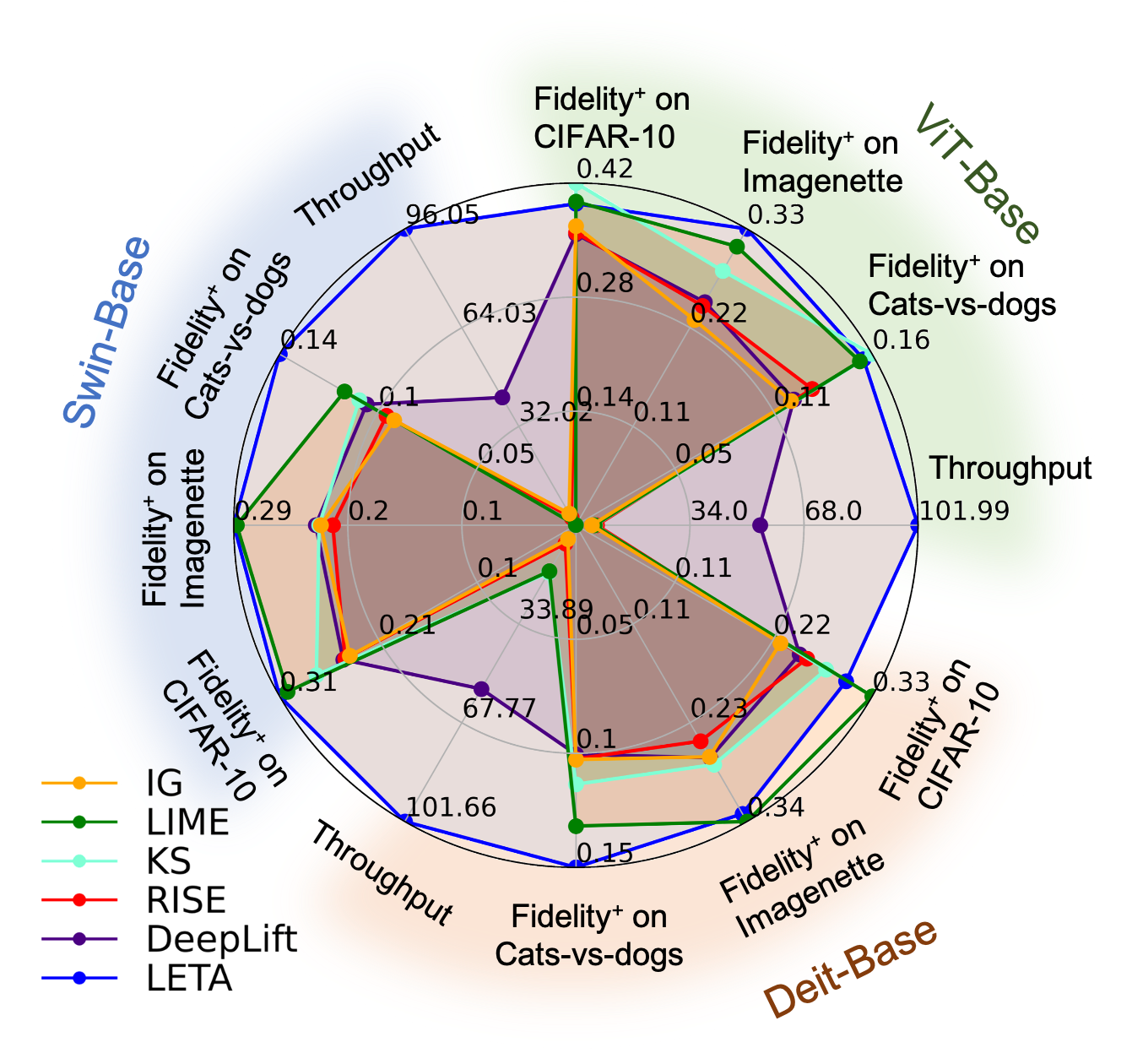
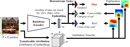
Figure 1: (a) Performance of LETA versus state-of-the-art baseline methods. (b) The transferable attribution encapsulates the explanation of elements in the image, which can explain various downstream tasks.

To solve this problem, we propose LEarning Transferable Attribution (LETA) aiming to develop a pre-trained, DNN-based, generic explainer based on large-scale image datasets, such that it can be seamlessly deployed across explaining various downstream tasks within the scope of pre-training data distribution. However, this introduces two non-trivial challenges. CH1: Enabling the explainer to effectively transfer across various downstream tasks without the task-specific knowledge for pre-training poses a significant challenge. CH2: Achieving the adaptation of the explainer to a particular downstream task without necessitating fine-tuning on the task-specific data introduces another challenge.

Our work effectively tackles these challenges. To address CH1, we propose a transferable attribution to guide pre-training the generic explainer on large-scale image datasets. The transferable attribution versatilely encodes the essential elements for explaining various downstream tasks via exhaustively attributing each dimension of instance embedding. After the pre-training, in response to CH2, we propose a rule-based approach to adapt the transferable attribution to downstream tasks, without the need for additional training on task-specific data. Moreover, we theoretically demonstrate the pre-training enables minimizing the explanation error bound aligned with the conditional $\mathcal{V}$-information on downstream tasks. Figure 1 shows the comprehensive performance of LETA pre-trained on the ImageNet dataset and deployed on the Cats-vs-dogs, Imagenette, and CIFAR-100 datasets, where LETA shows competitive fidelity and efficiency compared with state-of-the-art baseline methods. To summarize, our work makes the following contributions:

• We introduce a transferable attribution to guide the pre-training of generic explainer. Then, we propose a rule-based method to adopt the transferable attribution to explain downstream tasks within the scope of pre-training data distribution.

• We theoretically demonstrate the pre-training contributes to reducing the explanation error bound in downstream tasks, ensuring an alignment with the conditional $\mathcal{V}$-information on downstream tasks.

• Explaining three architectures of vision transformer on three downstream datasets, the experiment results indicate LETA can effectively explain the tasks without additional training on task-specific data.

2 Preliminary

In this section, we introduce the notations for problem formulation and concept of attribution transfer.

2.1 Notations

Target Model.

We focus on the explanation of vision models$:\mathcal{X}\to\mathcal{Y}_{t}$ in this work, where $\mathcal{X}=\mathbb{N}^{\mathrm{W}\times\mathrm{W}}$ denote the spatial space of $\mathrm{W}\times\mathrm{W}$ pixels; $\mathbb{N}$ denote the space of a single pixel with three channels; and $\mathcal{Y}_{t}$ denotes the label space. Moreover, we follow most of existing work [18, 17] and implementation of DNNs [40] to consider the target model as $f_{t}=H_{t}\circ G$, where the backbone encoder ${G}(\bullet):\mathbb{N}^{\mathrm{W}\times\mathrm{W}}\to\mathbb{R}^{\mathrm{D}}$ is pre-trained on large-scale datasets; and the classifier ${H}_{t}(\bullet):\mathbb{R}^{\mathrm{D}}\to\mathcal{Y}_{t}$ is finetuned on a specific task $t$. Although we follow the transfer learning setting [6, 18, 5] to freeze the backbone encoder ${G}(\bullet)$ during the task-specific fine-tuning. Our experiment results in Section 5.3 further show that the proposed generic explanation framework also shows effectiveness in the scenario where the target model is fully fine-tuned on downstream data.

Image Patch.

We follow existing work [27] to consider the patch-wise attribution of model prediction, i.e. the importance of each patch. Specifically, we follow existing work [8, 21] to split each image $\bm{x}_{k}$ into $\mathrm{P}\times\mathrm{P}$ patches in a grid pattern, where each patch has $\mathrm{C}\times\mathrm{C}$ pixels. Here, we have $\mathrm{W}=\mathrm{C}\mathrm{P}$. Let $\mathcal{Z}(\bm{x}_{k})=\{{z}_{i,j}\mid 1\leq i,j\leq\mathrm{P}\}$ denote the patches of an image $\bm{x}_{k}\in\mathcal{X}$, where a patch ${z}\in\mathbb{N}^{\mathrm{C}\times\mathrm{C}}$ aligns with continuous $\mathrm{C}\times\mathrm{C}$ pixels of the image. Moreover, we define $\mathcal{N}({z})\subseteq\mathcal{Z}(\bm{x}_{k})$ as the neighbors of a patch $z$ within the grid space, because a patch together with its neighbors have richer semantic content for model explanation. In our experiment, we follow the vision transformer [11] to split the image patches with $\mathrm{P}=14$ for $224\times 224$ input images from the ImageNet dataset; and we consider $\mathcal{N}({z})$ as the zero-, one-, and two-hop neighbors of the patch $z$.

Model Perturbation.

For a patch subset $\mathcal{S}\subseteq\mathcal{Z}(\bm{x}_{k})$, $f_{t}(\mathcal{S};\bm{x}_{k},y)$ represents the output of target model $f_{t}$ with a perturbed instance as the input. For the perturbed instance, the pixels belonging to the patches $z\in\mathcal{Z}(\bm{x}_{k})\setminus\mathcal{S}$ are removed and take $0$, which is approximately the average value of normalized pixels. e.g. $f_{t}(\mathcal{N}(z);\bm{x}_{k},y)$ defines the output of the target model based on the perturbed instance, where the pixels not belonging to the neighbors of patch $z$ are removed and take $0$.

Feature Attribution.

This work focuses on the feature attribution of target models for providing explanations. The feature attribution process involves generating importance scores, denoted as $\phi_{k,y,z}$ for each patch $z\in\mathcal{Z}(\bm{x}_{k})$ of the input image $\bm{x}_{k}\in\mathcal{X}$, to indicate its importance to the model prediction $f_{t}(\mathcal{Z}(\bm{x}_{k});\bm{x}_{k},y)$.

2.2 Advantages of Attribution Transfer

The motivation behind attribution transfer stems from model transfer in vision tasks. Specifically, it arises from the observation that a backbone encoder possesses the capability to capture essential features of input images and represent them as embedding vectors. This versatility enables the backbone to effectively adapt to a wide range of downstream tasks within the scope of pre-training data distribution. As shown in Figure 1, information of man, car, house encoded in the embedding vector enables the detection of genders, cars, and buildings in three different downstream scenarios, respectively. Despite the demonstrated transferability of the backbone encoder, existing research has challenges in achieving ’transferable explanation’ across different tasks. To bridge this gap and streamline the explanation process, we propose a transferable attribution that can be applied across various tasks, resulting in a significant reduction in the cost associated with generating explanations.

We define the transferable attribution as a tensor that versatilely encodes the essential attributions for explaining various downstream tasks. As shown in Figure 1, we illustrate the transferable attribution as a three-dimensional tensor. A simple and effective method proposed in this work is attributing the importance of input patches to each element of the embedding vector for transferable attribution. As shown in Figure 1, each $\mathrm{P}\times\mathrm{P}$ slice of this tensor corresponds to $\mathrm{P}\times\mathrm{P}$ patches within the input image, encoding their importance to a specific dimension of the embedding vector. In this way, the transferable attribution inherits the adaptability of the embedding vector, making it versatile enough to adapt various explanation tasks in downstream scenarios. e.g. the transferable attribution encodes the explanation of man and car for the embedding vector, such that it can transfer to explain the car classification and gender detection. The versatility of transferable attribution can effectively address the CH1 described in Section 1. We formalize the attribution transfer in Sections 3.

3 Definition of Attribution Transfer

In this section, we begin by following the $\mathcal{V}$-information theory to define the explanation. Then, we introduce the definition of transferable attribution in Definition 1. Finally, we propose a rule-based adaptation of transferable attribution to explaining specific downstream tasks in Definition 2.

3.1 Explanation by $\mathcal{V}$-Information

We formulate the importance of patch $z$ to a downstream model $f_{t}$ into the conditional mutual information between $\mathcal{N}(z)$ and $Y_{t}$, $I(\mathcal{N}(z);Y_{t}~{}|~{}B)$, given the state of remaining patches $B\subseteq\mathcal{Z}(\bm{x}_{k})\setminus\mathcal{N}(z)$ [3]. However, estimating this mutual information accurately poses a challenge due to the unknown distribution of $\mathcal{N}(z)$ and $B$. To address this challenge, we adopt an information-theoretic framework introduced in works by [41, 19], known to as conditional $\mathcal{V}$-information $I_{\mathcal{V}}(\mathcal{N}(z)\to Y_{t})$. In particular, conditional $\mathcal{V}$-information redirects the computation of mutual information to a certain predictive model within function space $\mathcal{V}$, as defined by:

$$I_{\mathcal{V}}(\mathcal{N}(z)\to Y_{t}~{}|~{}B)=H_{\mathcal{V}}(Y_{t}~{}|~{}B)-H_{\mathcal{V}}(Y_{t}~{}|~{}\mathcal{N}(z),B).$$ (1)

where $\mathcal{V}$-entropy $H_{\mathcal{V}}(Y_{t}~{}|~{}B)$ takes the lowest entropy over the function space $\mathcal{V}$, which is given by

$$H_{\mathcal{V}}(Y_{t}~{}|~{}B)=\inf_{f\in\mathcal{V}}\mathbb{E}_{y\sim\mathcal{Y}_{t}}[-\log f(B;\bm{x}_{k},y)].$$ (2)

Note that the $\mathcal{V}$-information explanation should align with a pre-trained target model $f_{t}\in\mathcal{V}$ and a specific class label $y$. The $\mathcal{V}$-entropy should take its value at $f_{t}$ and $y$, instead of the infimum expectation value, for the explanation. Therefore, we relax the $\mathcal{V}$-entropy terms $H_{\mathcal{V}}(Y_{t}~{}|~{}B)$ and $H_{\mathcal{V}}(Y_{t}~{}|~{}\mathcal{N}(z),B)$ into $-\log f_{t}(B;\bm{x}_{k},y)$ and $-\log f_{t}(\mathcal{N}(z)\cup B;\bm{x}_{k},y)$, respectively [14], for aligning the explanation with the target model $f_{t}\in\mathcal{V}$ and class label $y$. In this way, the attribution of patch $z$ aligned with class $y$ is defined as follows:

$$\phi_{k,y,{z}}=\mathbb{E}_{B\subseteq\mathcal{Z}(\bm{x}_{k})\setminus\mathcal{N}(z)}[-\log f_{t}(B;\bm{x}_{k},y)+\log f_{t}(\mathcal{N}(z)\cup B;\bm{x}_{k},y)].$$ (3)

It is impossible to enumerate the state of $B$ over $B\subseteq\mathcal{Z}(\bm{x}_{k})\setminus\mathcal{N}(z)$ in Equation (3). We follow existing work [28] to approximate it into two antithetical states to simplify the computation [28]. These cases involve considering the state of $B$ to be completely remaining patches $\mathcal{Z}(\bm{x}_{k})\setminus\mathcal{N}(z)$ or empty set $\varnothing$, narrowing down the enumeration of $B\subseteq\mathcal{Z}(\bm{x}_{k})\setminus\mathcal{N}(z)$ to $B\sim\{\mathcal{Z}(\bm{x}_{k})\setminus\mathcal{N}(z),\varnothing\}$ in Equation (3). Based on our numerical studies in Appendix C, the approximate attribution shows linear positive correlation with the exact value, which indicates the approximation does not affect the quality of attribution. To summarize, we approximate the attribution value of patch $z$ aligned with class $y$ as follows:

$$\phi_{k,y,{z}} \approx\mathbb{E}_{B\sim\{\mathcal{Z}(\bm{x}_{k})\setminus\mathcal{N}(z),\varnothing\}}[-\log f_{t}(B;\bm{x}_{k},y)+\log f_{t}(\mathcal{N}(z)\cup B;\bm{x}_{k},y)],$$ (4)

$$\sim\log f_{t}(\mathcal{N}(z);\bm{x}_{k},y)-\log f_{t}(\mathcal{Z}(\bm{x}_{k})\setminus\mathcal{N}(z);\bm{x}_{k},y),$$ (5)

where the terms $f_{t}(\mathcal{Z}(\bm{x}_{k});\bm{x}_{k},y)$ and $f_{t}(\varnothing;\bm{x}_{k},y)$ in Equation (4) are constant given $\bm{x}_{k}$ and $y$, thus being ormited in Equation (5). Intuitively, the explanation of patch $z$ depends on the gap of logit values, where $\mathcal{N}(z)$ and background patches $\mathcal{Z}(\bm{x}_{k})\setminus\mathcal{N}(z)$ are taken as the input.

3.2 Transferable Attribution

We introduce the concept of transferable attribution, formally defined in Definition 1. Note that Equation (5) relies on the downstream classifier $f_{t}$, which is task-related. The purpose of transferable attribution is to disentangle the task-specific aspect of the attribution from Equation (5). This disentanglement renders the attribution task independent and suitable for deployment across various tasks.

Definition 1 (Transferable Attribution).

Given a backbone encoder $G$, the transferable attribution for a patch $z\in\mathcal{Z}(\bm{x}_{k})$, $\bm{x}_{k}\in\mathcal{X}$, is represented by two tensors $\textbf{{g}}_{k,z}$ and $\textbf{{h}}_{k,z}$ as follows:

$$\textbf{{g}}_{k,z} ={G}(\mathcal{N}({z});\bm{x}_{k}),$$

$$\textbf{{h}}_{k,z} ={G}(\mathcal{Z}(\bm{x}_{k})\setminus\mathcal{N}({z});\bm{x}_{k}).$$ (6)

Definition 1 is derived using the backbone encoder $G$, facilitating its application across different tasks. Moreover, let $\textbf{{g}}_{k}=[\textbf{{g}}_{k,z}~{}|~{}z\in\mathcal{Z}(\bm{x}_{k})]$ and $\textbf{{h}}_{k}=[\textbf{{h}}_{k,z}~{}|~{}z\in\mathcal{Z}(\bm{x}_{k})]$ denote the transferable attribution for the instance $\bm{x}_{k}$, which is a collection of patch-level transferable attribution given in Definition 1. Representing the transferable attribution for instance $\bm{x}_{k}$, $\textbf{{g}}_{k}$ and $\textbf{{h}}_{k}$ are 3D tensors in the shape of $\mathrm{P}\times\mathrm{P}\times\mathrm{D}$, where $\mathrm{D}$ denotes the output dimension of the backbone encoder $G$, as defined in Section 2.1.

3.3 Adaptation to Task-aligned Explanation

For explaining downstream tasks, we propose a rule-based method in Definition 1 to generate the task-aligned explanation from the transferable attribution. The rule-based adaptation can effectively address the CH2 described in Section 1, without the need for additional training on task-specific data.

Definition 2 (Attribution Transfer).

If the task-specific function is given by $f_{t}=H_{t}\circ G$, then the explanation of $f_{t}(\bm{x}_{k})$ is generated by

$$\phi_{k,y,{z}}=\log H_{t}(\textbf{{g}}_{k,z};y)-\log H_{t}(\textbf{{h}}_{k,z};y),$$ (7)

where $\textbf{{g}}_{k,z}$ and $\textbf{{h}}_{k,z}$ are the transferable attribution for patch $z\in\mathcal{Z}(\bm{x}_{k})$; and $G$ and $H$ represent the backbone encoder and fine-tuned classifier on the specific task, respectively.

Following Definitions 1 and 2, it is straightforward to achieve $\phi_{k,y,z}=\log H_{t}(\textbf{{g}}_{k,z};y)-\log H_{t}(\textbf{{h}}_{k,z};y)=\log f_{t}(\mathcal{N}(z);\bm{x}_{k},y)-\log f_{t}(\mathcal{Z}(\bm{x}_{k})\setminus\mathcal{N}(z);\bm{x}_{k},y)$. This adaptation to $\phi_{k,y,z}$ can effectively explain downstream task $t$ following the definition of conditional $\mathcal{V}$-information $I_{\mathcal{V}}(\mathcal{N}(z)\to Y_{t}~{}|~{}B)$, as described in Section 3.1.

4 Learning Transferable Attribution

In this section, we introduce LEarning Transferable Attribution (LETA). Specifically, LETA focus on pre-training a DNN-based generic explainer $E(\bullet~{}|~{}\theta)$ to learn the knowledge of transferable attribution proposed in Definition 1 on large-scale image dataset. After this, LETA deploys the generic explainer $E(\bullet~{}|~{}\theta)$ to downstream tasks for end-to-end generating task-aligned explanation, which is significantly more efficient than individual explaining the tasks. Finally, we theoretically study the explanation error bound of LETA in Theorem 1.

4.1 Explainer Pre-training Aims for Transferable Attribution

LETA employs a generic explainer $E(\bullet~{}|~{}\theta)$ to generate the transferable attribution. Following Definition 1, $E(\bullet\mid\theta)$ yields two tensors for transferable attribution, $\hat{\textbf{{g}}}_{k}$ and $\hat{\textbf{h}}_{k}$, represented as $[\hat{\textbf{{g}}}_{k},\hat{\textbf{h}}_{k}]=E(\bm{x}_{k}\mid\theta)$. Specifically, $\hat{\textbf{{g}}}_{k}$ and $\hat{\textbf{h}}_{k}$ are $\mathrm{P}\times\mathrm{P}\times\mathrm{D}$ tensors consisting of $\hat{\textbf{{g}}}_{k}=[\hat{\textbf{{g}}}_{k,z}\in\mathbb{R}^{\mathrm{D}}~{}|~{}z\in\mathcal{Z}(\bm{x}_{k})]$ and $\hat{\textbf{h}}_{k}=[\hat{\textbf{h}}_{k,z}\in\mathbb{R}^{\mathrm{D}}~{}|~{}z\in\mathcal{Z}(\bm{x}_{k})]$, respectively. Each of the slices $\hat{\textbf{{g}}}_{k,z}$ and $\hat{\textbf{h}}_{k,z}$ corresponds to a patch $z$ of the input image, towards the predction of transferable attribution $\textbf{{g}}_{k,z}$ and $\textbf{h}_{k,z}$, respectively. Pursuant to this objective, LETA learns the parameters of $E(\bullet\mid\theta)$ to minimize the loss function as follow:

$$\mathcal{L}_{\theta}(\bm{x}_{k})=\mathbb{E}_{{z}\sim\mathcal{Z}(\bm{x}_{k})}\big{[}||\hat{\textbf{{g}}}_{k,{z}}-\textbf{{g}}_{k,{z}}\big{|}\big{|}_{2}^{2}+\big{|}\big{|}\hat{\textbf{h}}_{k,{z}}-\textbf{h}_{k,{z}}||_{2}^{2}\big{]},$$ (8)

where $\textbf{{g}}_{k,{z}}$ and $\textbf{h}_{k,{z}}$ are given by Definition 1.

Algorithm 1 Pre-training of $E(\bullet\mid\theta)$

Input: Pre-training dataset $\mathcal{D}$.
Output: Generic explainer $E(\bullet\mid\theta^{*})$.

1:  for $\bm{x}_{k}\sim\mathcal{D}$ do

2:     Sample patches ${z}\sim\mathcal{Z}(\bm{x}_{k})$.

3:     Generate $\textbf{{g}}_{k,z}$ and $\textbf{h}_{k,{z}}$ following Def. 1.

4:     Update $E(\bullet|\theta)$ to minimize Eq. (8).

5:  end for

Algorithm 1 summarizes one epoch of pre-training the generic explainer $E(\bullet\mid\theta)$. Specifically, LETA first samples a mini-batch of image patches (lines 2); then estimates the transferable attribution following Definition 1 (lines 3); finally updates the parameters of $E(\bullet\mid\theta)$ to minimize the loss function given by Equation (8) (line 4). The iteration ends with the convergence of the $E(\bullet\mid\theta)$. According to Algorithm 1, the pre-training of generic explainer $E(\bullet~{}|~{}\theta)$ towards the output of generic encoder $G$ instead of specific tasks. This empowers the trained $E(\bullet~{}|~{}\theta)$ to remain impartial towards specific tasks, providing the flexibility for seamless adaptation across diverse downstream tasks.

4.2 Generating Task-aligned Explanation

On the deployment, LETA follows Definition 2 to explain downstream tasks. Specifically, to explain a downstream task inference $(H_{t}\circ G)(\bm{x}_{k})$, LETA first generates transferable attribution from the pre-trained generic explainer $[\hat{\textbf{{g}}}_{k},\hat{\textbf{h}}_{k}]=E(\bm{x}_{k}\mid\theta)$; then takes the patch-level attribution $\hat{\textbf{{g}}}_{k,z}$ and $\hat{\textbf{h}}_{k,z}$ into Equation (7). To summarize, LETA generates the explanation for a patch $z\in\mathcal{Z}(\bm{x}_{k})$ by

$$\hat{\phi}_{k,y,{z}}=\log H_{t}(\hat{\textbf{{g}}}_{k,z};y)-\log H_{t}(\hat{\textbf{h}}_{k,z};y).$$ (9)

Let $\hat{\bm{\phi}}_{k,y}=[\hat{\phi}_{k,y,z}~{}|~{}z\in\mathcal{Z}(\bm{x}_{k})]$ denote the $\mathrm{P}\times\mathrm{P}$ explanation heatmap for image $\bm{x}_{k}$, where each element $\hat{\phi}_{k,z}$ is given by Equation (9), indicating the importance of all patches in $\bm{x}_{k}$. LETA can efficiently generate the explanation heatmap $\hat{\bm{\phi}}_{k}$ for image $\bm{x}_{k}$ through matrix multiplication as follows,

$$\hat{\bm{\phi}}_{k,y}=\log H_{t}(\hat{\textbf{{g}}}_{k};y)-\log H_{t}(\hat{\textbf{h}}_{k};y).$$ (10)

In particular, the classifier $H_{t}(\bullet;y)$ in Equation (10) is related with task $t$. This enables the explanation to align with task $t$ without the need for additional training of the explainer on the downstream data.

4.3 Theoretical Analysis

We theoretically study the estimation error of $\hat{\phi}_{k,y,{z}}$ with respect to $\phi_{k,y,{z}}$. Specifically, we begin by considering an ideal scenario where $\mathcal{L}_{\theta}(\bm{x}_{k})\to 0$. Under these conditions, it follows that $\hat{\textbf{{g}}}_{k,z}\to\textbf{{g}}_{k,z}$ and $\hat{\textbf{h}}_{k,z}\to\textbf{h}_{k,z}$. Then, the ratios $\frac{{H}_{t}(\hat{\textbf{{g}}}_{k,z};y)}{{H}_{t}(\textbf{{g}}_{k,z};y)}\to 1$ and $\frac{{H}_{t}(\textbf{h}_{k,z};y)}{{H}_{t}(\hat{\textbf{h}}_{k,z};y)}\to 1$ are established. In this context, it is straightforward to have $|\hat{\phi}_{k,y,{z}}-\phi_{k,y,{z}}|\to 0$, which indicates the explanation $\hat{\phi}_{k,y,{z}}$ converges towards the exact $\phi_{k,y,{z}}$ in the ideal scenario. Without loss of generality, we also consider the scenario where $\mathcal{L}_{\theta}(\bm{x}_{k})\to 0$ is not met. In this case, we consider the ratios $\frac{{H}_{t}(\hat{\textbf{{g}}}_{k,z};y)}{{H}_{t}(\textbf{{g}}_{k,z};y)}$ and $\frac{{H}_{t}(\textbf{h}_{k,z};y)}{{H}_{t}(\hat{\textbf{h}}_{k,z};y)}$ may not precisely equal 1. Instead, we allow for a range $1-\epsilon\leq\frac{{H}_{t}(\hat{\textbf{{g}}}_{k,z};y)}{{H}_{t}(\textbf{{g}}_{k,z};y)},\frac{{H}_{t}(\textbf{h}_{k,z};y)}{{H}_{t}(\hat{\textbf{h}}_{k,z};y)}\leq 1+\epsilon$, where $0\leq\epsilon\ll 1$. Under these conditions, we establish the estimation error bound of $\phi_{k,y,z}$ in Theorem 1, with a detailed proof in Appendix B. This allows us to provide a comprehensive understanding of the estimation accuracy even when the ideal scenario of $\mathcal{L}_{\theta}(\bm{x}_{k})\to 0$ is not met.

Theorem 1 (Explanation Error Bound).

Given the classifier ${H}_{t}(\bullet)$ of the downstream task, if the output of classifier ${H}_{t}(\hat{\textbf{{g}}}_{k,z};y)$ and ${H}_{t}(\hat{\textbf{h}}_{k,z};y)$ fall within the range of $1-\epsilon\leq\frac{{H}_{t}(\hat{\textbf{{g}}}_{k,z};y)}{{H}_{t}(\textbf{{g}}_{k,z};y)},\frac{{H}_{t}(\textbf{h}_{k,z};y)}{{H}_{t}(\hat{\textbf{h}}_{k,z};y)}\leq 1+\epsilon$, then, the upper bound of explanation error is given by

$$\mathbb{E}_{\bm{x}_{k}\sim\mathcal{D}_{t},y\sim\mathcal{Y}_{t},{z}\sim\mathcal{Z}(\bm{x}_{k})}|\hat{\phi}_{k,y,{z}}-\phi_{k,y,{z}}|\leq\frac{2\epsilon}{1-\epsilon},$$ (11)

where $\hat{\phi}_{k,y,{z}}$ and $\phi_{k,y,{z}}$ are given by Equation (9) and (7), respectively; and $\mathcal{D}_{t}$ denotes the downstream dataset.

Intuition of Theorem 1.

During the pre-training of LETA, the estimation of $\hat{\textbf{{g}}}_{k,z}$ and $\hat{\textbf{h}}_{k,z}$ gradually approaches their exact values $\textbf{{g}}_{k,z}$ and $\textbf{h}_{k,z}$, respectively, as a result of the loss value $\mathcal{L}_{\theta}(\bm{x}_{k})$ approaching its minimum value. This causes a reduction of $\epsilon$ because the ratios $\frac{{H}_{t}(\hat{\textbf{{g}}}_{k,z};y)}{{H}_{t}(\textbf{{g}}_{k,z};y)}$ and $\frac{{H}_{t}(\textbf{h}_{k,z};y)}{{H}_{t}(\hat{\textbf{h}}_{k,z};y)}$ gradually converge to a narrower range around 1. This reduction in $\epsilon$ explicitly lowers the estimation error bound $\frac{2\epsilon}{1-\epsilon}$ compared with the conditional $\mathcal{V}$-information attribution on downstream tasks. This underscores the effectiveness of LETA pre-training the generic explainer $E(\bullet\mid\theta)$ in enhancing explanations for downstream tasks.

5 Experiment Results

In this section, we conduct experiments to evaluate LETA by answering the following research questions: RQ1: How does LETA perform compared with state-of-the-art baseline methods in terms of the fidelity? RQ2: How does LETA perform in explaining fully fine-tuned target model on down-stream datasets? RQ3: How is the transferability of LETA across different down-stream datasets? RQ4: Do both pre-training and attribution transfer in LETA contribute to explaining down-stream tasks?

5.1 Experiment Setup

We provide the details about benchmark datasets, baseline methods, evaluation metrics, and implementation details in this section.

Datasets.

We consider the large-scale ImageNet dataset [10] for LETA pre-training. Moreover, we adopt the Cats-vs-dogs [13], CIFAR-100 [24], and Imagenette [20] datasets for the downstream task of explanation. More details about the datasets are given in Appendix F.

Baseline Methods.

We consider seven baseline methods for comparison, which include general explanation methods: LIME [30], IG [36], RISE [29], and DeepLift [1]; Shapley explanation methods: KernelSHAP (KS) [27], and GradShap [27]; and DNN-based explainer: ViT-Shapley [9] in our experiment. More details about the baseline methods are given in Appendix G.

Evaluation Metrics.

We consider the fidelity to evaluate the explanation following existing work [43, 8]. Specifically, the fidelity evaluates the explanation via removing the important or trivial patches from the input instance and collecting the prediction difference of the target model $f_{t}$. These two perspectives of evluation are formalized into $\mathrm{Fidelity}^{+}$ and $\mathrm{Fidelity}^{-}$, respectively. Specifically, provided a subset of patches $\mathcal{S}^{*}\subseteq\mathcal{Z}(\bm{x}_{k})$ that are important to the target model $f_{t}$ by an explanation method, the $\mathrm{Fidelity}^{+}$ and $\mathrm{Fidelity}^{-}$ evaluates the explanation following

$$\uparrow\mathrm{Fidelity}^{+}=\frac{1}{|\mathcal{D}_{\text{task}}|}\sum_{\bm{x}\in\mathcal{D}_{\text{task}}}f_{t}(\mathcal{Z}(\bm{x}_{k});\bm{x}_{k},y)-f_{t}(\mathcal{Z}(\bm{x}_{k})\setminus\mathcal{S}^{*};\bm{x}_{k},y),$$ (12)

$$\downarrow\mathrm{Fidelity}^{-}=\frac{1}{|\mathcal{D}_{\text{task}}|}\sum_{\bm{x}\in\mathcal{D}_{\text{task}}}f_{t}(\mathcal{Z}(\bm{x}_{k});\bm{x}_{k},y)-f_{t}(\mathcal{S}^{*};\bm{x}_{k},y).$$ (13)

Higher $\mathrm{Fidelity}^{+}$ indicates a better explanation for prediction $y$, since the truly important patches of image $\bm{x}_{k}$ have been removed, leading to a significant difference of model prediction. Moreover, lower $\mathrm{Fidelity}^{-}$ implies a better explanation for prediction $y$, since the truly important patches have been preserved in $\mathcal{S}^{*}$ to keep the prediction similar to the original one. The fidelity should be compared at the same level of sparsity $|\mathcal{S}^{*}|/|\mathcal{U}|$. Consequently, we consider the evaluation of fidelity versus the sparsity in most cases.

Target Models.

For downstream classification tasks, we comprehensively consider three architectures of vision transformers as the backbone encoders, including the ViT-Base/Large [11], Swin-Base/Large [26], Deit-Base [37] transformers. The classification models (to be explained) consist of one of the backbone encoders with ImageNet pre-trained weights and a linear classifier. For the task-specific fine-tuning of target models, we consider two mechanisms: classifier-tuning and full-fine-tuning. Specifically, the classifier-tuning follows the transfer learning setting [6, 18, 5] to freeze the parameters of backbone encoder during the fine-tuning; and the full-fine-tuning updates all parameters during the finetuning. Note that the classifier-tuning can not only be more efficient but also prevent the over-fitting problem on downstream data due to fewer trainable parameters [35]. We consider the classifier-tuning for most of our experiments including Sections 5.2, 5.4, 5.5, and 5.7; and consider the full-fine-tuning in Section 5.3; while these two mechanisms yield the same result for Section 5.6. The hyper-parameters of task-specific fine-tuning are given in Appendix H.

Hyper-parameter Settings.

The experiment follows the pipeline of LETA pre-training, explanation generation and evaluation on multiple downstream datasets. Specifically, LETA adopts the Mask-AutoEncoder [17] as the backbone, followed by a multiple Feed-Forward (FFN) layers to generate the transferable attribution. More details about the explainer backbone, explainer architecture and hyper-parameters of LETA pre-training are given in Appendix H. When deploying LETA to explaining downstream tasks, the explanation is aligned with the classification result of the target model.

5.2 Evaluation of Fidelity (RQ1)

In this section, we evaluate the fidelity of LETA under the classifier-tuning setting. Due to the space constraints, we present 18 figures illustrating the $\mathrm{Fidelity}^{+}$-sparsity curve and the $\mathrm{Fidelity}^{-}$-sparsity curve for explaining the ViT-Base, Swin-Base, and Deit-Base model prediction on the Cats-vs-dogs, Imagenette, and CIFAR-10 datasets in Appendix D. To streamline our evaluation, we simplify the assessment of fidelity-sparsity curves by calculating its Area Under the Curve (AUC) over the sparsity from zero to one, which aligns with the average fidelity value. Intuitively, a higher $\mathrm{Fidelity}^{+}$-sparsity-AUC($\uparrow$) indicates superior $\mathrm{Fidelity}^{+}$ performance across most sparsity levels, reflecting a more faithful explanation. Similarly, a lower $\mathrm{Fidelity}^{-}$-sparsity-AUC($\downarrow$) signifies a more faithful explanation. More details about the fidelity-sparsity-AUC are given in Appendix E. On the Cats-vs-dogs, Imagenette, and CIFAR-10 datasets, we present the $\mathrm{Fidelity}^{+}$-sparsity-AUC($\uparrow$) for explanations in Figures 2 (a)-(c), respectively, as well as the $\mathrm{Fidelity}^{-}$-sparsity-AUC($\downarrow$) in Figures 2 (e)-(g), respectively. We have the following observations:

• LETA consistently exhibits promising performance in terms of both $\mathrm{Fidelity}^{+}$($\uparrow$) and $\mathrm{Fidelity}^{-}$($\downarrow$) scores, surpassing the majority of baseline methods. This underscores LETA’s ability to faithfully explain various downstream tasks within the scope of pre-training data distribution.

• LETA exhibits significant strengths in both $\mathrm{Fidelity}^{+}$($\uparrow$) and $\mathrm{Fidelity}^{-}$($\downarrow$), highlighting its effectiveness in identifying both important and non-important features. In contrast, the baseline methods struggle to simultaneously achieve high $\mathrm{Fidelity}^{+}$ and low $\mathrm{Fidelity}^{-}$. e.g. consider LIME’s performance when explaining the Deit-Base model on the CIFAR-10 dataset. While LIME excels in $\mathrm{Fidelity}^{+}$, it falls short in $\mathrm{Fidelity}^{-}$.

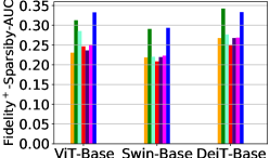
(a) Imagenette

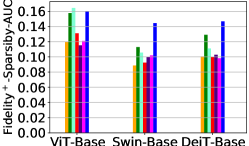
(b) Cats-vs-dogs

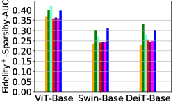
(c) CIFAR-10

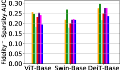
(d) Imagenette

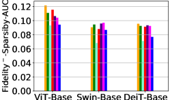
(e) Cats-vs-dogs

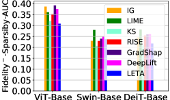
(f) CIFAR-10

Figure 2: $\mathrm{Fidelity}^{+}$-Sparsity-AUC($\uparrow$) on the Imagenette (a), Cat-vs-dogs (b), and CIFAR-10 (c) datasets. $\mathrm{Fidelity}^{-}$-Sparsity-AUC($\downarrow$) on the Imagenette (d), Cat-vs-dogs (e), and CIFAR-10 (f) datasets.

5.3 Adaptation to Fully Fine-tuned Models (RQ2)

In this section, we evaluate the fidelity of LETA under the full-fine-tuning setting to demonstrate its generalization ability. Notably, the ViT-Base classification model including both the backbone and classifier are fine-tuned on downstream data, which are not available to LETA pre-training. The explanation considers three methods: learning from scratch (LFScratch), LETA pre-training (LETA-PT), and LETA fine-tuning (LETA-FT). To adapt to the fully fine-tuned target model, LFScratch trains the explainer on the downstream dataset for one epoch; LETA-PT simply transfers the pre-trained explainer to explaining the down-stream tasks; LETA-FT follows Algorithm 1 to fine-tune the explainer using the fine-tuned backbone encoder on the downstream dataset for one epoch. Here, we consider the Imagenette and Cat-vs-dogs datasets for the downstream tasks. Further details about fine-tuning the target models and explainers are given in Appendix H. The loss value of LFScratch and LETA-FT versus the epochs are shown in Figures 3 (a) and (d). The fidelity-sparsity curves of all methods are given in Figures 3 (b), (c), (e), and (f). We have the following observations:

• LETA pre-training provides a good initial explainer for adaption to fully fine-tuned encoders. According to Figures 2 (a,d), the LETA pre-trained explainer shows lower training loss than learning from scratch in the early epochs. This indicates the pre-training provides a good initialization for the adaptation.

• LETA-PT can effectively explain the fully fine-tuned target model, even without fine-tuning. According to Figures 2 (b,c,e,f), LETA-PT shows competitive fidelity when comparing with LETA-FT and other baseline methods, and a significant improvement over LFScratch. This indicates the strong generalization ability of LETA, which derives from being pre-trained on the large-scale dataset, ImageNet.

• The fine-tuning of backbone encoder and generic explainer can be executed independently and parallelly. Specifically, LETA pre-trains the generic explainer based on open-sourced pre-trained backbone encoders; meanwhile, the encoder can be fine-tuned independently in downstream tasks. This can significantly improve the efficiency and flexibility of deploying LETA to practical scenarios.

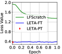
(a) Imagenette

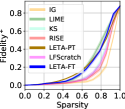
(b) Imagenette

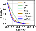
(c) Imagenette

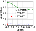
(d) Cats-vs-dogs

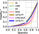
(e) Cats-vs-dogs

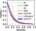
(f) Cats-vs-dogs

​​​​ ​​​​ ​​​​ ​​​​ ​​​​

Figure 3: Fine-tuning loss value versus epoch on the Imagenette (a) and Cats-vs-dogs (d) datasets. $\mathrm{Fidelity}^{+}$($\uparrow$) versus Sparsity on the Imagenette (b) and Cats-vs-dogs (c) datasets. $\mathrm{Fidelity}^{-}$($\downarrow$) versus Sparsity on the Imagenette (e) and Cats-vs-dogs (f) datasets.

5.4 Evaluation of Transferability (RQ3)

Table 1: Explanation $\mathrm{Fidelity}^{+}$-Sparsity-AUC($\uparrow$) and $\mathrm{Fidelity}^{-}$-Sparsity-AUC($\downarrow$) for Deit-Base, Swin-Base, and Deit-Base target models on the Cat-vs-dogs, Imagenette, and CIFAR-10 datasets.

	Datasets	Cats-vs-dogs		Imagenette		CIFAR-10
Target Model	Method	$\mathrm{Fidelity}^{+}$($\uparrow$)	$\mathrm{Fidelity}^{-}$($\downarrow$)	$\mathrm{Fidelity}^{+}$($\uparrow$)	$\mathrm{Fidelity}^{-}$($\downarrow$)	$\mathrm{Fidelity}^{+}$($\uparrow$)	$\mathrm{Fidelity}^{-}$($\downarrow$)
ViT-Base	ViTShapley	0.11$\pm$0.09	0.13$\pm$0.10	0.25$\pm$0.13	0.25$\pm$0.14	0.36$\pm$0.17	0.36$\pm$0.17
	LETA-$H_{\textsl{g}}$	0.14$\pm$0.11	0.10$\pm$0.08	0.29$\pm$0.14	0.18$\pm$0.10	0.39$\pm$0.18	0.34$\pm$0.17
	LETA	0.16$\pm$0.13	0.09$\pm$0.07	0.33$\pm$0.16	0.19$\pm$0.12	0.40$\pm$0.18	0.31$\pm$0.16
Swin-Base	ViTShapley	0.09$\pm$0.05	0.11$\pm$0.07	0.24$\pm$0.07	0.24$\pm$0.09	0.25$\pm$0.11	0.28$\pm$0.14
	LETA-$H_{\textsl{g}}$	0.14$\pm$0.09	0.10$\pm$0.07	0.29$\pm$0.08	0.24$\pm$0.07	0.26$\pm$0.12	0.27$\pm$0.13
	LETA	0.14$\pm$0.10	0.09$\pm$0.05	0.29$\pm$0.10	0.22$\pm$0.06	0.31$\pm$0.14	0.24$\pm$0.12
DeiT-Base	ViTShapley	0.12$\pm$0.08	0.1$\pm$0.07	0.22$\pm$0.09	0.29$\pm$0.11	0.28$\pm$0.13	0.24$\pm$0.13
	LETA-$H_{\textsl{g}}$	0.13$\pm$0.08	0.09$\pm$0.06	0.33$\pm$0.10	0.25$\pm$0.08	0.32$\pm$0.14	0.24$\pm$0.13
	LETA	0.15$\pm$0.10	0.08$\pm$0.06	0.33$\pm$0.10	0.24$\pm$0.08	0.30$\pm$0.13	0.22$\pm$0.12

We evaluate the transferability of LETA compared with ViT-Shapley [9], a state-of-the-art DNN-based explainer for vision models. Although ViT-Shapley cannot explain multiple tasks, we pre-train the explainer of ViT-Shapley on the large-scale ImageNet dataset, and transfer it to the Cat-vs-dogs, Imagenette, and CIFAR-10 datasets without additional training. The same procedure is applied to LETA. Moreover, we also consider a LETA-$H_{\textsl{g}}$ method to study whether the pre-training of LETA contributes to explaining downstream tasks. To be concrete, LETA takes a task-specific classifier $H_{t}$ into Definition 2; while LETA-$H_{\textsl{g}}$ takes a general classifier (pre-trained on the ImageNet dataset). We follow Section 5.2 to adopt the fidelity-sparsity AUC to evaluate the average fidelity. Table 1 illustrates the fidelity for explaining the ViT-Base, Swin-Base, and Deit-Base models on the Cat-vs-dogs, Imagenette, and CIFAR-10 datasets. We have the insights:

• LETA shows stronger transferability than ViT-Shapley. Note that the explainer of LETA and ViT-Shapley are pre-trained on the ImageNet dataset, and transferred to the downstream datasets without additional training. LETA shows higher $\mathrm{Fidelity}^{+}$($\uparrow$) and lower $\mathrm{Fidelity}^{-}$($\downarrow$) than ViT-Shapley.

• The pre-training of LETA significantly contributes to explaining downstream tasks. LETA-$H_{\textsl{g}}$ adopts the generally pre-trained explainer and classifier to explain downstream tasks, and achieves a reasonable fidelity on most of the datasets. This indicates the pre-training of LETA captures the transferable features across various datasets for explaining downstream tasks.

• It is more faithful to explain downstream tasks based on the task-specific classifiers. LETA outperforms LETA-$H_{\textsl{g}}$ on most architectures and datasets, which indicates the attribution transfer had better take a classifier aligned with a downstream task for $H_{t}$ in Definition 2.

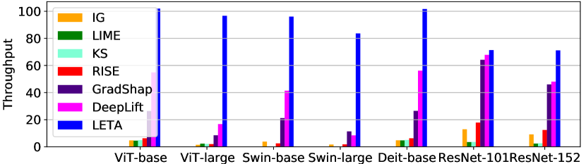
Figure 4: Throughput of explaining different architectures.

​​​​

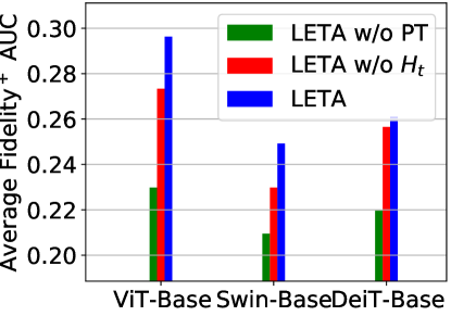
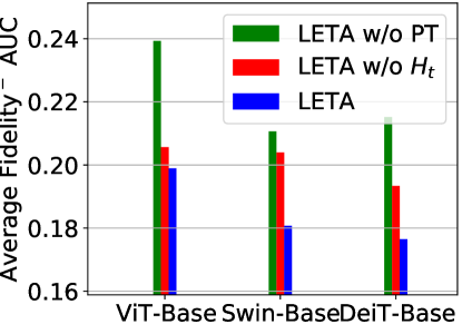
Figure 5: Fidelity of ablation studies.

5.5 Ablation Studies (RQ4)

We ablatedly study the contribution of the key steps in LETA to explaining down-stream tasks, including the pre-training of generic explainer and attribution transfer aligned to each task. For our evaluation, we consider three methods: LETA w/o Pre-training (PT), LETA w/o $H_{t}$, and LETA. Specifically, for LETA w/o PT, the generic explainer is randomly initialized without pre-training, and attribution transfer follows Definition 2. For LETA w/o $H_{t}$, the generic explainer is pre-trained following Algorithm 1, and the explanation for each task is generated by $\hat{\bm{\phi}}_{k}=\log H_{\textsl{g}}(\hat{\textbf{{g}}}_{k};y)-\log H_{\textsl{g}}(\hat{\textbf{h}}_{k};y)$, where $H_{\textsl{g}}$ takes a general classifier pre-trained on the ImageNet datasets, instead of being fine-tuned corresponding to the task. Figures 5 illustrates the $\mathrm{Fidelity}^{+}$-Sparsity-AUC($\uparrow$) and $\mathrm{Fidelity}^{-}$-Sparsity-AUC($\downarrow$) associated with each method, where the fidelity score represents the averaged value on the Cats-vs-dogs, Imagenette, and CIFAR-10 datasets. Other configurations remain consistent with Appendix H. Overall, we have the following observations:

• LETA pre-training significantly contributes to explaining the downstream tasks. This can be verified by the degradation of fidelity observed from LETA w/o PT in Figures 5 (b) and (c).

• The classifier $H_{t}$ for attribution transfer should align with the explaining task $t$. LETA achieves better fidelity than LETA w/o $H_{t}$ according to Figures 5 (b) and (c). This indicates the task-aligned $H_{t}$ is better than the general classifier $H_{\textsl{g}}$ for the attribution transferred to a specific task.

5.6 Evaluation of Latency

In this section, we evaluate the latency of LETA compared with baseline methods. Specifically, we adopt the metric $\mathrm{Throughput}=\frac{N_{\text{test}}}{T}$($\uparrow$) to evaluate the explanation latency, where $N_{\text{test}}$ represents the number of testing instances and $T$ signifies the total time consumed during the explanation process. In our experiments, we measure throughput while explaining predictions made by ViT-Base/Large, Swin-Base/Large, Deit-Base, ResNet-101/152 models on the ImageNet dataset, as shown in Figure 5. Detailed information about our computational infrastructure configuration is given in Appendix 4. Overall, we observe:

• LETA is more efficient than state-of-the-art baseline methods, by generating explanations through a single feed-forward pass of the explainer. In contrast, the baseline methods rely on multiple samplings of the forward or backward passes of the target model, resulting in a considerably slower explanation process.

  Among the baseline methods, KernelSHAP exhibits similar $\mathrm{Fidelity}^{-}$($\downarrow$) compared to LETA, as shown in Figure 2, its significantly lower throughput limits its practicality in real-world scenarios.

• LETA exhibits the most negligible decrease in throughput as the size of the target model grows, as seen when transitioning from ViT-Base to ViT-Large. This advantage stems from the fact that LETA’s latency is contingent upon the explainer’s model size, rather than the target model.

  In contrast, the baseline methods suffer from notable performance slowdown as the size of the target model increases. Our analysis reveals that the speed of the baseline methods decreases in tandem with the target model’s size due to the necessity of sampling the target model to generate explanations.

5.7 Case Studies

​​​ ​​​ ​​​

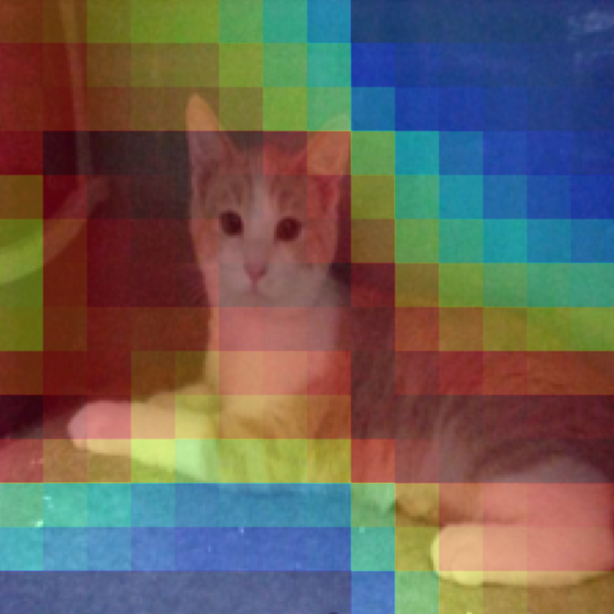
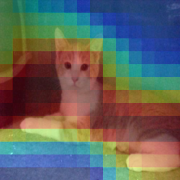
(a) Cats

​​​ ​​​ ​​​

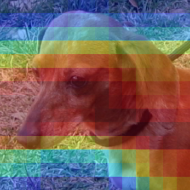
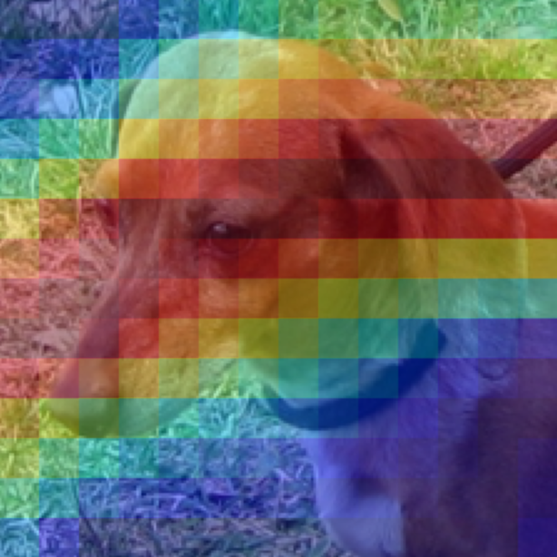
(b) Dogs

​​​ ​​​ ​​​

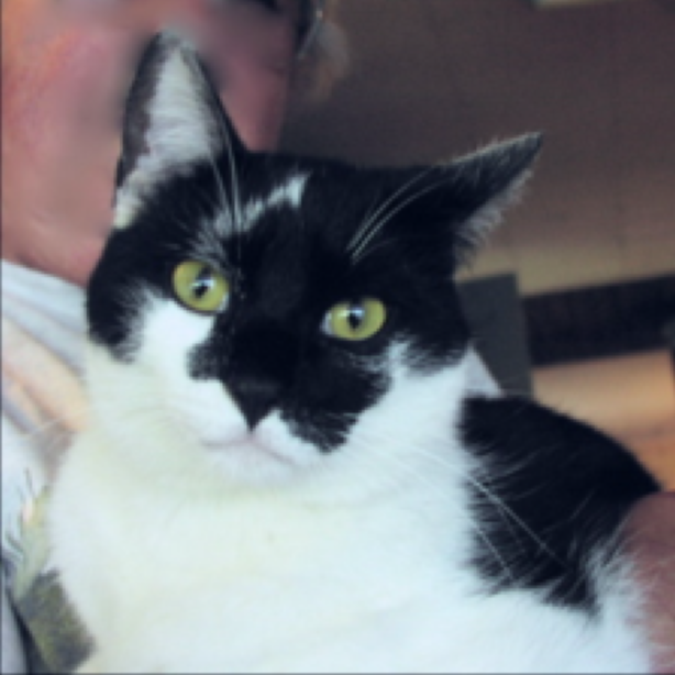
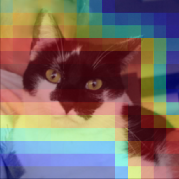
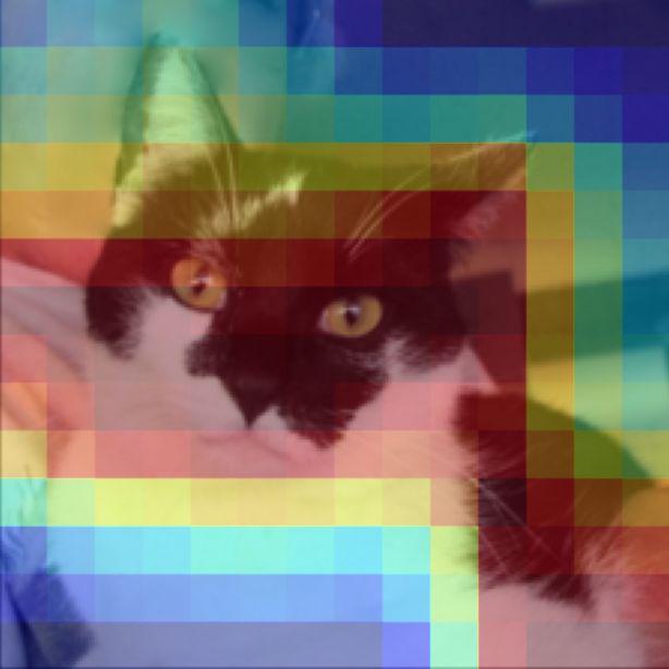
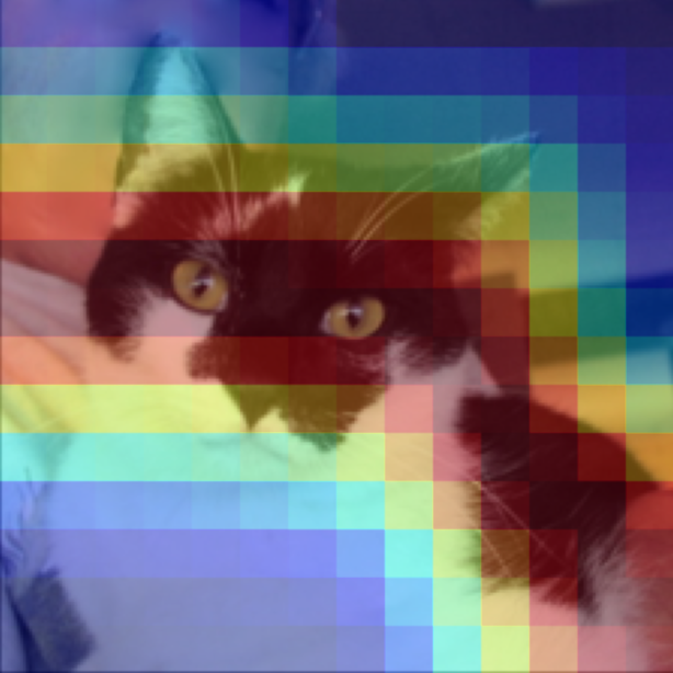
(c) Cats

​​​ ​​​ ​​​

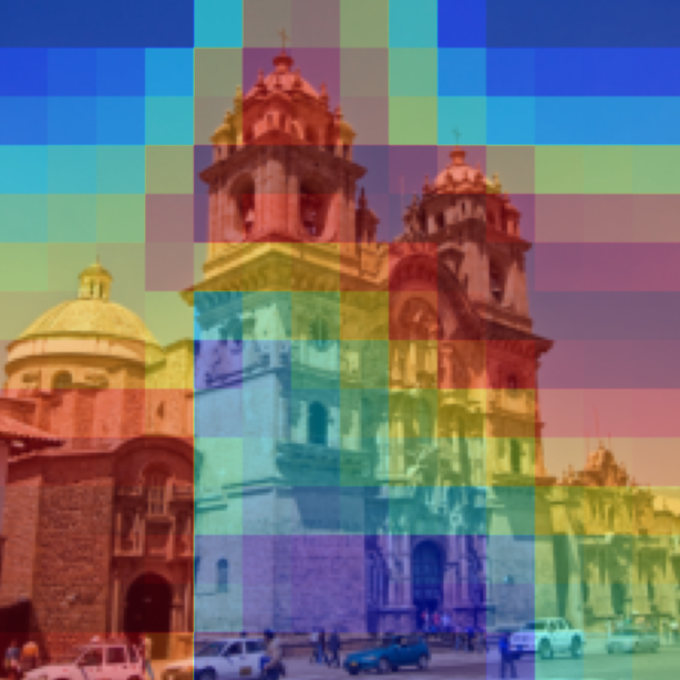
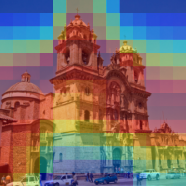
(d) Church

​​​ ​​​ ​​​

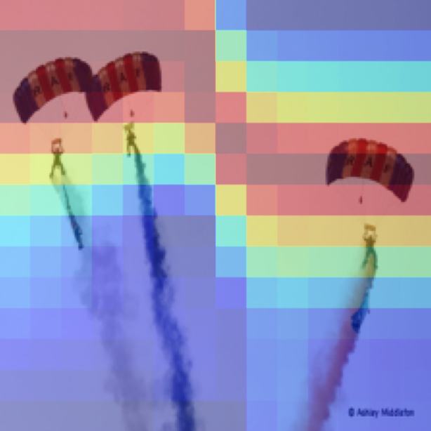
(e) Parachute

​​​ ​​​ ​​​

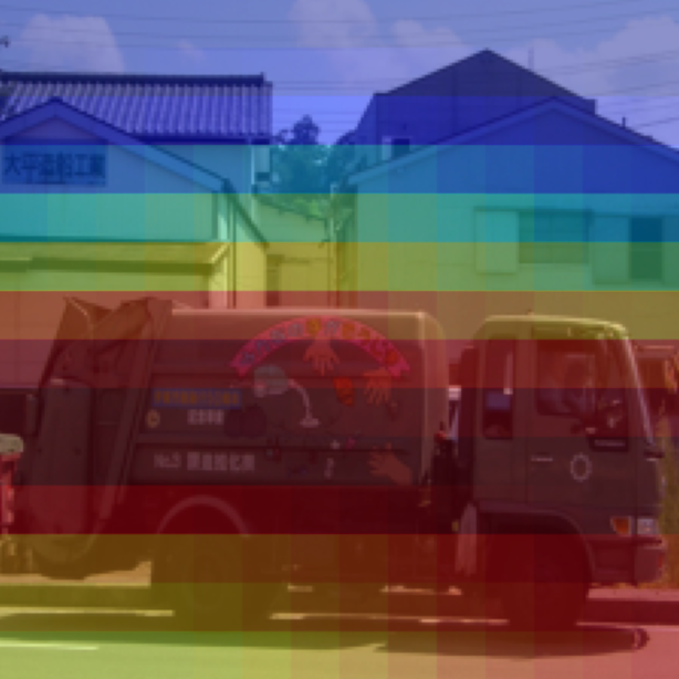
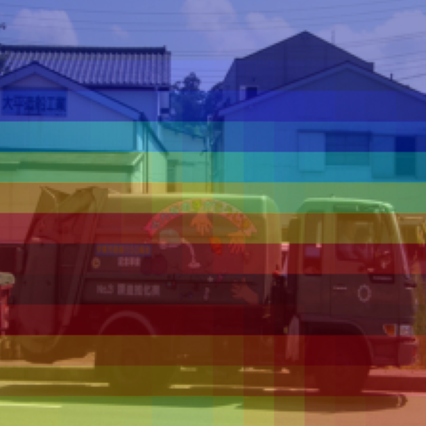
(f) Garbage truck

​​​ ​​​ ​​​

(g) Ship

​​​ ​​​ ​​​

(h) Airplane

​​​ ​​​ ​​​

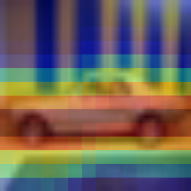
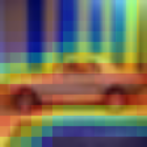
(i) Automobile

Figure 6: Visualization of explanation on the Cats-vs-dogs (a)-(c), Imagenette (d)-(e), and CIFAR-10 (g)-(i) datasets. In each subgraph, from the left-side to the right-side, the three heatmaps explain the inference of the Swin-Base, Deit-Base, and Deit-Base model, respectively.

​​​​​​ ​​​​​​
​​​​​​ ​​​​​​
​​​​​​ ​​​​​​

In this section, we visualize the explanations generated by LETA, demonstrating its power in helping human users understand vision models. Specifically, we randomly sample 100 instances from the Cats-vs-dogs, Imagenette, and CIFAR-10 datasets, and visualize the explanations of Swin-Base, Deit-Base, and Deit-Base models in Figure 6(a), where subgraphs (a)-(c), (d)-(f), and (g)-(i) correspond to the Cats-vs-dogs, Imagenette, and CIFAR-10 datasets, respectively. In each subgraph, from the left-side to the right-side, the three heatmaps explain the inference of the Swin-Base, Deit-Base, and Deit-Base model, respectively. Notably, LETA generates the explanation heatmap in an end-to-end manner without pre- or post-processing. More case studies are shown in Appendix J. According to the case study, we observe:

• The salient patches emphasized by LETA’s explanation reveal semantically meaningful patterns. e.g. as depicted in Figure 6(a) (d), (e), and (g), the Swin-Base model concentrates on the tower, canopy and bow, respectively, to identify a church, parachute, and ship.

• LETA does not rely on pre-processing of the image or post-processing of the explanation heatmap. In contrast, existing work EAC [34] requires SAM [22] to segment the input image, which is less flexible than LETA.

• Different model architectures make predictions based on distinct image elements. e.g. as illustrated in Figure 6(a) (g), the Swin-Base and Deit-Base models primarily emphasize the ship’s bow for identification. In contrast, the Deit-Base model takes into account the ship’s keel for its predictions.

6 Conclution

In this work, we propose LETA, a pre-trained, DNN-based, generic explanation framework for vision models. Specifically, LETA guides the pre-training of the generic explainer to learn the transferable attribution, and introduces a rule-based attribution transfer for explaining downstream tasks. Notably, LETA conducts the pre-training and attribution transfer without the need for task-specific training data, enabling easy and flexible deployment across various downstream tasks. Our theoretical analysis verifies that the pre-training of LETA contributes to minimizing the explanation error bound compared with the conditional $\mathcal{V}-$information on downstream tasks. Moreover, experiment results demonstrate that the pre-training of LETA can effectively explain the models fine-tuned in various downstream scenarios, achieving competitive results compared with state-of-the-art explanation methods.

Appendix

Appendix A Related Work

Explainable machine learning (ML) has made significant advancements, leading to model transparency and better human understanding of deep neural networks (DNNs) [12]. Specifically, existing work of explainable ML can be categorized into two groups: local explainers and DNN-based explainers [7].

Local Explainer.

Local explainer focuses on constructing local explanation based on perturbation of the target black-box model, like KernelSHAP [27], LIME [30], GradCAM [32], and Integrated Gradient [36]. Specifically, KernelSHAP approximates the Shapleyvalue by learning an explainable surrogate (linear) model based on the DNN output of reference input for each feature; LIME generates the explanation by sampling points around the input instance and using DNN output at these points to learn a surrogate (linear) model; Integrated Gradients estimates the explanation by the integral of the gradients of DNN output with respect to the inputs, along the pathway from specified references to the inputs. These pieces of work rely on resource-intensive procedures like sampling or backpropagation of the target black-box model [25], leading to undesirable trade-off between the efficiency and interpretation fidelity [7].

DNN-based Explainer.

This branch of work leverages the training process to acquire proficiency in constructing a DNN-based explainer, utilizing explanation values as training labels [7]. This innovative strategy empowers the simultaneous generation of explanations for an entire batch of instances through a single, streamlined feedforward operation of the DNN-based explainer. Exemplifying this progress are innovative approaches like FastSHAP [21], ViT-Shapley [9], CORTX [8], LARA [31, 38], and HarsanyiNet [4]. To be concrete, FastSHAP and ViT-Shapley adopt a DNN as the explainer to learn the Shapley value, which relies on task-specific training and cannot be transferred across different tasks; and CoRTX arguments the training of DNN-based explainer through a contrastive pre-training framework, and adopt the true Shapley value to fine-tune the explainer. The DNN-based explainer have played a pivotal role in significantly streamlining the deployment of DNN explanations within real-time applications. However, they are constrained to explaining individual black box models, and they lack the ability to transfer the explanation across various models and tasks. This limitation results in the explanation of various tasks in practical scenarios becoming time- and resource-consuming due to the necessity of training different explainers for each task.

Appendix B Proof of Theorem 1

We prove Theorem 1 in this section.

Theorem 1 (Explanation Error Bound).

Given the classifier ${H}_{t}(\bullet)$ of the downstream task, if the output of classifier ${H}_{t}(\hat{\textbf{{g}}}_{k,z};y)$ and ${H}_{t}(\hat{\textbf{h}}_{k,z};y)$ fall within the range of $1-\epsilon\leq\frac{{H}_{t}(\hat{\textbf{{g}}}_{k,z};y)}{{H}_{t}(\textbf{{g}}_{k,z};y)},\frac{{H}_{t}(\textbf{h}_{k,z};y)}{{H}_{t}(\hat{\textbf{h}}_{k,z};y)}\leq 1+\epsilon$, then, the upper bound of explanation error is given by

$$\mathbb{E}_{\bm{x}_{k}\sim\mathcal{D}_{t},y\sim\mathcal{Y}_{t},{z}\sim\mathcal{Z}(\bm{x}_{k})}|\hat{\phi}_{k,y,{z}}-\phi_{k,y,{z}}|\leq\frac{2\epsilon}{1-\epsilon},$$ (14)

where $\hat{\phi}_{k,y,{z}}$ and $\phi_{k,y,{z}}$ are given by Equation (9) and (7), respectively; and $\mathcal{D}_{t}$ denotes the downstream dataset.

Proof.

To achieve the explanation error bound, we first have the upper bound of $\hat{\phi}_{k,y,z}-\phi_{k,y,z}$ given by

$$\hat{\phi}_{k,y,z}-\phi_{k,y,z} =\log H_{t}(\hat{\textbf{{g}}}_{k,z};y)-\log H_{t}(\textbf{{g}}_{k,z};y)+\log H_{t}(\textbf{{h}}_{k,z};y)-\log H_{t}(\hat{\textbf{{h}}}_{k,z};y),$$ (15)

$$=\log\frac{H_{t}(\hat{\textbf{{g}}}_{k,z};y)}{H_{t}(\textbf{{g}}_{k,z};y)}+\log\frac{H_{t}(\textbf{{h}}_{k,z};y)}{H_{t}(\hat{\textbf{{h}}}_{k,z};y)}\leq\frac{H_{t}(\hat{\textbf{{g}}}_{k,z};y)}{H_{t}(\textbf{{g}}_{k,z};y)}-1+\frac{H_{t}(\textbf{{h}}_{k,z};y)}{H_{t}(\hat{\textbf{{h}}}_{k,z};y)}-1,$$ (16)

$$\leq\frac{H_{t}(\hat{\textbf{{g}}}_{k,z};y)}{H_{t}(\textbf{{g}}_{k,z};y)}-1+\frac{H_{t}(\textbf{{h}}_{k,z};y)}{H_{t}(\hat{\textbf{{h}}}_{k,z};y)}-1\leq\epsilon+\epsilon,$$ (17)

Then, we have the lower bound of $\hat{\phi}_{k,y,z}-\phi_{k,y,z}$ as follows,

$$\hat{\phi}_{k,y,z}-\phi_{k,y,z} =-\log\frac{H_{t}(\textbf{{g}}_{k,z};y)}{H_{t}(\hat{\textbf{{g}}}_{k,z};y)}-\log\frac{H_{t}(\hat{\textbf{{h}}}_{k,z};y)}{H_{t}(\textbf{{h}}_{k,z};y)}\geq 1-\frac{H_{t}(\textbf{{g}}_{k,z};y)}{H_{t}(\hat{\textbf{{g}}}_{k,z};y)}+1-\frac{H_{t}(\hat{\textbf{{h}}}_{k,z};y)}{H_{t}(\textbf{{h}}_{k,z};y)},$$ (18)

$$=2-\bigg{(}\frac{H_{t}(\textbf{{g}}_{k,z};y)}{H_{t}(\hat{\textbf{{g}}}_{k,z};y)}+\frac{H_{t}(\hat{\textbf{{h}}}_{k,z};y)}{H_{t}(\textbf{{h}}_{k,z};y)}\bigg{)}\geq 2-\frac{1}{1-\epsilon}-\frac{1}{1-\epsilon}=\frac{-2\epsilon}{1-\epsilon}$$ (19)

Combining Equations (17) and (19), we achieve the upper bound of estimation error given by

$$|\hat{\phi}_{k,y,z}-\phi_{k,y,z}|\leq\max\Big{\{}2\epsilon,\frac{2\epsilon}{1-\epsilon}\Big{\}}=\frac{2\epsilon}{1-\epsilon}.$$ (20)

∎

Appendix C Approximation of Attribution

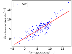
(a) Sampling number 16

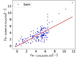
(b) Sampling number 16

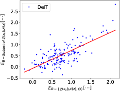
(c) Sampling number 16

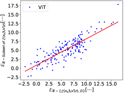
(d) Sampling number 32

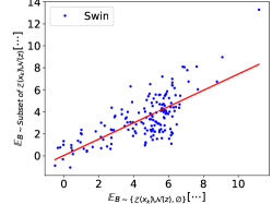
(e) Sampling number 32

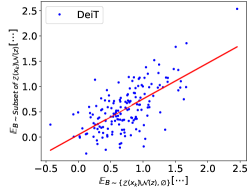
(f) Sampling number 32

Figure 7: $\mathbb{E}_{B\sim\text{Subset of }\mathcal{Z}(\bm{x}_{k})\setminus\mathcal{N}(z),\varnothing}[\cdots]$ versus $\mathbb{E}_{B\sim\{\mathcal{Z}(\bm{x}_{k})\setminus\mathcal{N}(z),\varnothing\}}[\cdots]$, where $\cdots$ is the abbreviation of $-\log f_{t}(B;\bm{x}_{k},y)+\log f_{t}(\mathcal{N}(z)\cup B;\bm{x}_{k},y)$; and $f_{t}$ takes the trained ViT-Base(a, d), Swin-Base(b, e), and Deit-Base(c, f) models on the ImageNet dataset. The sampling number of $B\sim\text{Subset of }\mathcal{Z}(\bm{x}_{k})\setminus\mathcal{N}(z)$ is 16 and 32 for Subfigures (a)-(c) and (d)-(f), respectively.

We conduct experiments to study the relationship between the approximate attribution $\mathbb{E}_{B\sim\{\mathcal{Z}(\bm{x}_{k})\setminus\mathcal{N}(z),\varnothing\}}[\cdots]$ and its exact value $\mathbb{E}_{B\sim\text{Subset of }\mathcal{Z}(\bm{x}_{k})\setminus\mathcal{N}(z)}[\cdots]$ on the ImageNet dataset, where $\cdots$ is the abbreviation of $-\log f_{t}(B;\bm{x}_{k},y)+\log f_{t}(\mathcal{N}(z)\cup B;\bm{x}_{k},y)$. Specifically, we collect the samples of $\mathbb{E}_{B\sim\{\mathcal{Z}(\bm{x}_{k})\setminus\mathcal{N}(z),\varnothing\}}[\cdots]$ and $\mathbb{E}_{B\sim\text{Subset of }\mathcal{Z}(\bm{x}_{k})\setminus\mathcal{N}(z)}[\cdots]$, where $\bm{x}_{k}$ take 100 instances randomly sampled from the ImageNet dataset; and the target models $f_{t}$ take the ViT-Base(a, d), Swin-Base(b, e), and Deit-Base(c, f) models trained on the ImageNet dataset. The samples of $\mathbb{E}_{B\sim\text{Subset of }\mathcal{Z}(\bm{x}_{k})\setminus\mathcal{N}(z)}[\cdots]$ versus $\mathbb{E}_{B\sim\{\mathcal{Z}(\bm{x}_{k})\setminus\mathcal{N}(z),\varnothing\}}[\cdots]$ is plotted in Figure 7. It is observed that the value of $\mathbb{E}_{B\sim\{\mathcal{Z}(\bm{x}_{k})\setminus\mathcal{N}(z),\varnothing\}}[\cdots]$ after the approximation shows positive linear correlation with $\mathbb{E}_{B\sim\text{Subset of }\mathcal{Z}(\bm{x}_{k})\setminus\mathcal{N}(z)}[\cdots]$. This indicates the approximate value $\mathbb{E}_{B\sim\{\mathcal{Z}(\bm{x}_{k})\setminus\mathcal{N}(z),\varnothing\}}[\cdots]$ can take the place of $\mathbb{E}_{B\sim\text{Subset of }\mathcal{Z}(\bm{x}_{k})\setminus\mathcal{N}(z)}[\cdots]$ for the function of attribution.

Appendix D Fidelity-Sparsity Curve

We show the fidelity-sparsity curve for explaining ViT-Base, Swin-Base, and Deit-Base on the Cats-vs-dogs, Imagenette, and CIFAR-10 datasets in Figure LABEL:fig:fidelity_curve (a)-(r). It is observed that LETA consistently exhibits promising performance in terms of both $\mathrm{Fidelity}^{+}$($\uparrow$) and $\mathrm{Fidelity}^{-}$($\downarrow$), surpassing the majority of baseline methods. This indicates LETA’s ability to faithfully explain various downstream tasks.

Appendix E Details about the Fidelity-sparsity-AUC Metric

We give details about the metrics $\mathrm{Fidelity}^{+}$-sparsity-AUC and $\mathrm{Fidelity}^{-}$-sparsity-AUC in this section. In Section 5.1, we have shown that higher $\mathrm{Fidelity}^{+}$ and lower $\mathrm{Fidelity}^{-}$ at the same level of sparsity indicate more faithful explanation. To streamline the evaluation, the assessment of fidelity-sparsity curves can be simplified into its Area Under the Curve (AUC) over the sparsity from zero to one, as shown in Figure 9 (a) and (b). The Fidelity-sparsity-AUC aligns with the average fidelity value. Specifically, a higher $\mathrm{Fidelity}^{+}$-sparsity-AUC ($\uparrow$) indicates better $\mathrm{Fidelity}^{+}$ performance across most sparsity levels, reflecting a more faithful explanation. Similarly, a lower $\mathrm{Fidelity}^{-}$-sparsity-AUC signifies a more faithful explanation For the given example in Figure 9 (a) and (b), explanation A is more faithful than B.

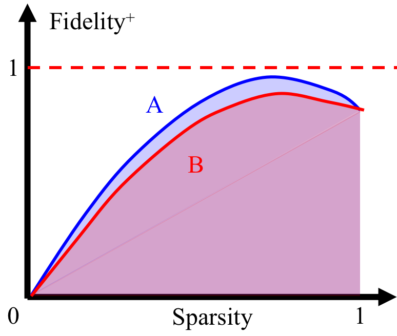
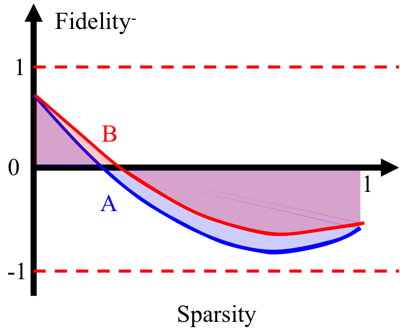
Figure 9: Illustration of $\mathrm{Fidelity}^{+}$-sparsity-AUC (a) and $\mathrm{Fidelity}^{-}$-sparsity-AUC (b)

Appendix F Details about the Datasets

We give the details about the datasets in this section. ImageNet: A large scale image dataset which has over one million color images covering 1000 categories, where each image has $224\!\times\!224$ pixels. Cats-vs-dogs: A dataset of cats and dogs images. It has 25000 training instances and 12500 testing instances. CIFAR-10: An image dataset with 60,000 color images in 10 different classes, where each image has $32\!\times\!32$ pixels. Imagenette: A benchmark dataset of explainable machine learning for vision models. It contains 10 classes of the images from the Imagenet.

Appendix G Details about the Baseline Methods

We give the details about the baseline methods in this section. ViT-Shapley: This work adopts vision transformers as the explainer to learn the Shapley value. This work is task-specific and cannot be transferred accross different tasks. RISE: RISE randomly perturbs the input, and average all the masks weighted by the perturbed DNN output for the final saliency map. The sampling number takes the default value $50$. IG: Integrated Gradients estimates the explanation by the integral of the gradients of DNN output with respect to the inputs, along the pathway from specified references to the inputs. DeepLift: DeepLift generates the explanation by decomposing DNN output on a specific input by backpropagating the contributions of all neurons in the network to every feature of the input. KernelSHAP: KernelSHAP approximates the Shapley value by learning an explainable surrogate (linear) model based on the DNN output of reference input for each feature. The sampling number takes the default value $25$ for each instance according to the captum.ai [23]. GradShap: GradShap estimates the importance features by computing the expectations of gradients by randomly sampling from the distribution of references. LIME [30]: LIME generates the explanation by sampling points around the input instance and using DNN output at these points to learn a surrogate (linear) model. The sampling number takes the default value $25$ according to the captum.ai. For implementation, we take the IG, DeepLift, and GradShap algorithms on the captum.ai, where the multiply_by_inputs factor takes false to achieve the local attribution for each instance.

Appendix H Implementation Details

We give the details about LETA pre-training and target model training on each downstream datasets in H.1 and H.2, respectively.

H.1 LETA Pretraining

We comprehensively consider three backbones for providing the generic attribution, including the ViT-Base/Large, Swin-Base/Large, Deit-Base transformers. Their pre-trained weights are loaded from the HuggingFace library [39]. The hyper-parameter setting of LETA pre-training is given in Table 2.

The architecture of the generic explainer is shown in Figure 10 (a). Specifically, the explainer adopts the Mask-AutoEncoder [17] for the backbone. The architecture of Mask-AutoEncoder is shown in Figure 11. More details about the Mask-AutoEncoder can be referred to its source code. Since the output shape of the Mask-AutoEncoder $[\mathrm{BS},\mathrm{P}\times\mathrm{P},768]$ is not matched with that of the generic attribution $[\mathrm{BS},\mathrm{P}\times\mathrm{P},\mathrm{D}]$, where $\mathrm{BS}$ denotes the mini-batch size. It adopts $n\times$ FFN-layers for the explainer head, where we found $n=17$ shows strong generalization ability in our experiments. The structure of an explainer head is given in Figure 10 (b). The first explainer head does not have the skip connection due to the mismatch of tensor shapes. The last explainer head does not have the GELU activation.

Target Encoder	ViT-Base	Swin-Base	DeiT-Base
Explainer Architecture	Figure 10
Pixel # per image $\mathrm{W}\times\mathrm{W}$	$224\times 224$
Patch # per image $\mathrm{P}\times\mathrm{P}$	$14\times 14$
Pixel # per patch $\mathrm{C}\times\mathrm{C}$	$16\times 16$
Shape of $\textbf{{g}}_{k}$ and $\textbf{h}_{k}$	$14\times 14\times 768$	$14\times 14\times 1024$	$14\times 14\times 768$
Optimizer	ADAM
Learning rate	$1\times 10^{-3}$
Mini-batch size	64
Scheduler	CosineAnnealingLR
Warm-up-ratio	0.05
Weight-decay	0.05
Epoch	50
Hops of neighbors	0, 1, 2

Table 2: Hyper-parameters of LETA pre-training on the ImageNet dataset.

H.2 Target Models in Downstream Tasks

The classification models (to be explained) consist of the backbones of ViT-Base/Large, Swin-Base/Large, Deit-Base transformers, and a linear classifier that has been fine-tuned on the Cats-vs-dogs, CIFAR-10, and Imagenette datasets, respectively. The hyper-parameters of fine-tuning the classifier of target models on each datasets are given in Table 3.

Datasets	Cats-vs-dogs	CIFAR-10	Imagenette
Target Backbone	ViT-Base, Swin-Base, and Deit-Base
Classifier	Linear classifier
Optimizer	ADAM
Learning rate	$2\times 10^{-4}$
Mini-batch size	256
Scheduler	Linear
Warm-up-ratio	0.05
Weight-decay	0.05
Epoch	5

Table 3: Hyper-parameters of training the target model.

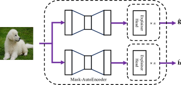
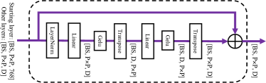
Figure 10: Generic explainer architecture. (a) Explainer architecture. (b) FFN-layers for the explainer head.

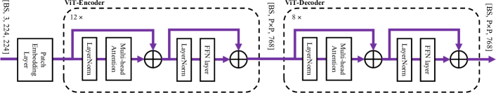
Figure 11: Structure of Mask-Autoencoder.

Appendix I Computational Infrastructure

The computational infrastructure information is given in Table 4.

Table 4: Computing infrastructure for the experiments.

Device Attribute	Value
Computing infrastructure	GPU
GPU model	NVIDIA-A5000
GPU Memory	24564MB
GPU Number	8
CUDA Version	12.1
CPU Memory	512GB

Appendix J More Case Studies

We give more explanation heatmaps of ViT-Base on the ImageNet dataset in Figures 12, which are generated by LETA.

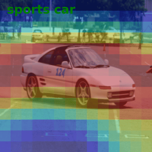
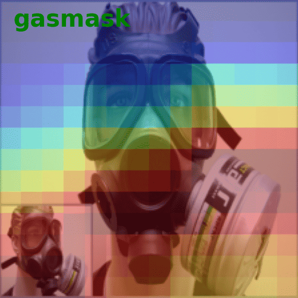
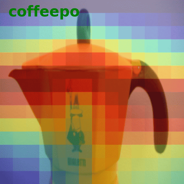
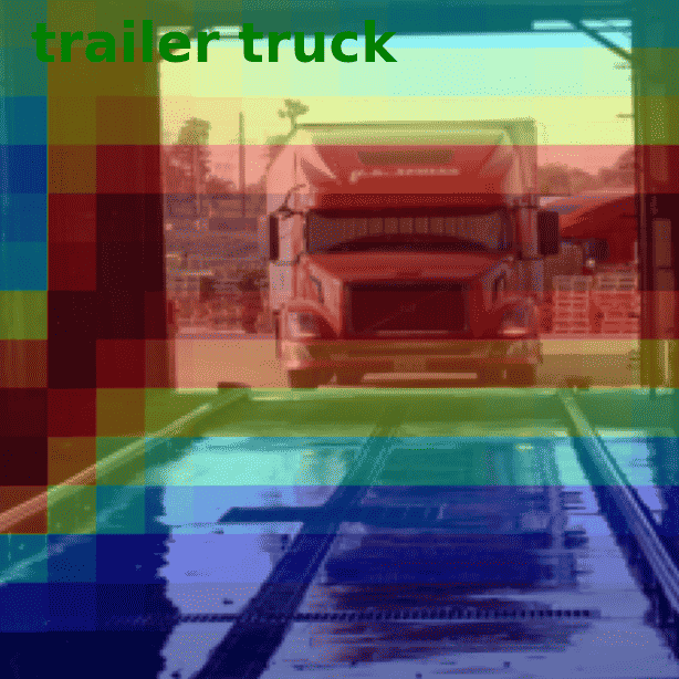
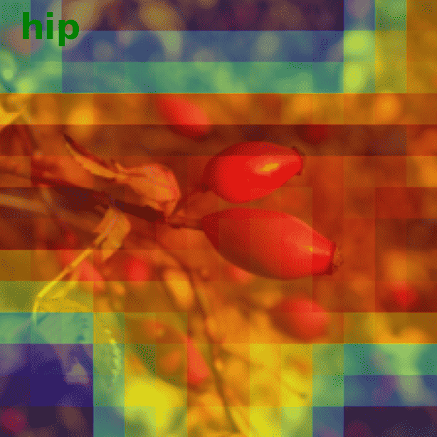
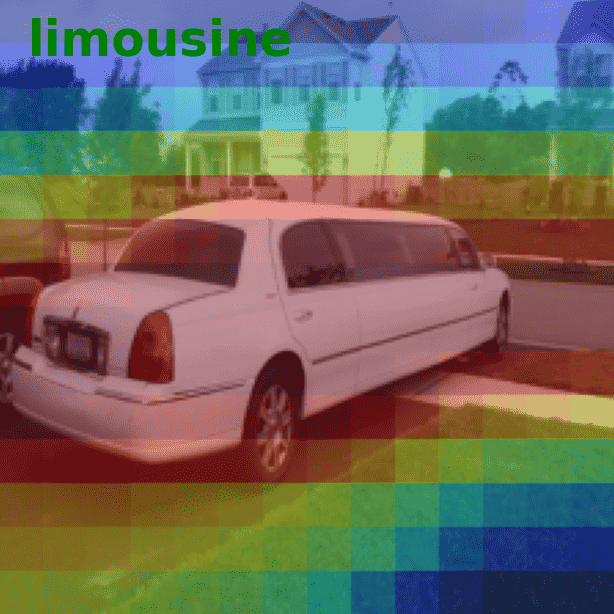
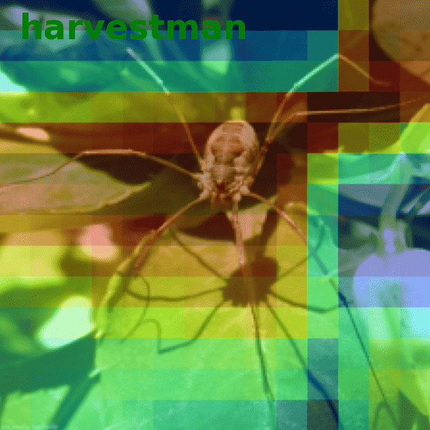
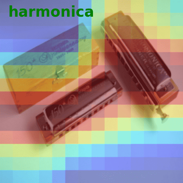
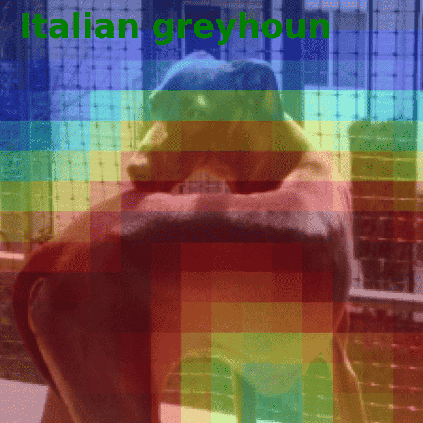
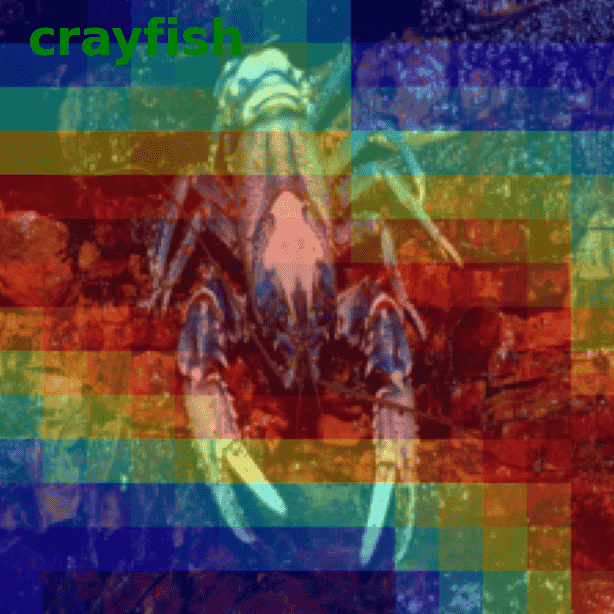
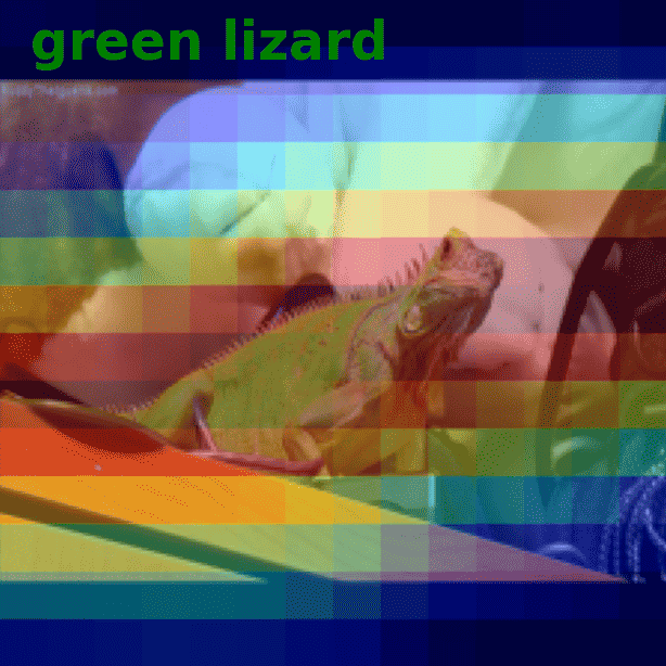
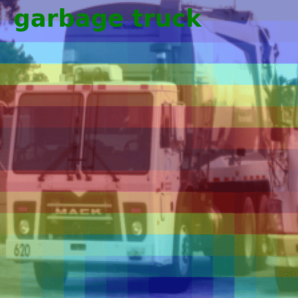
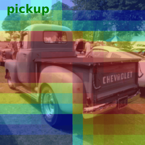
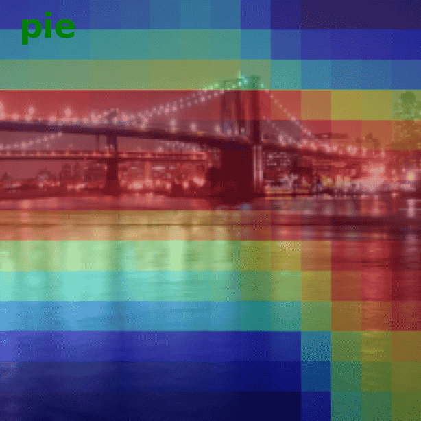
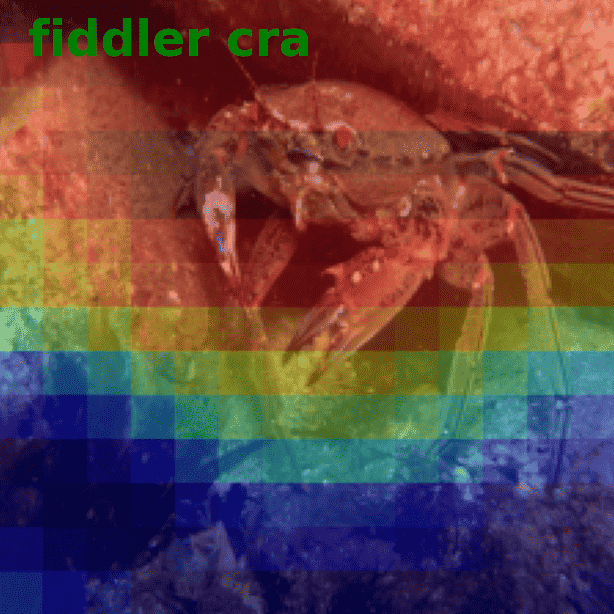
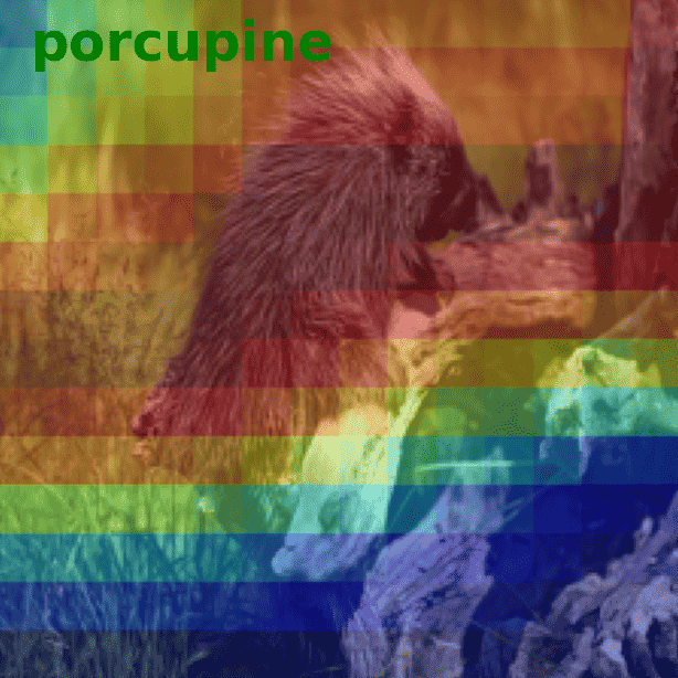
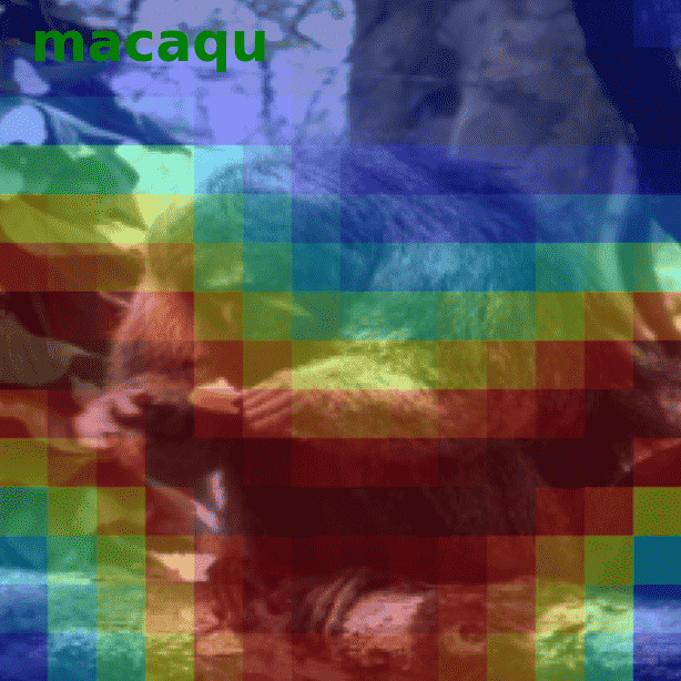
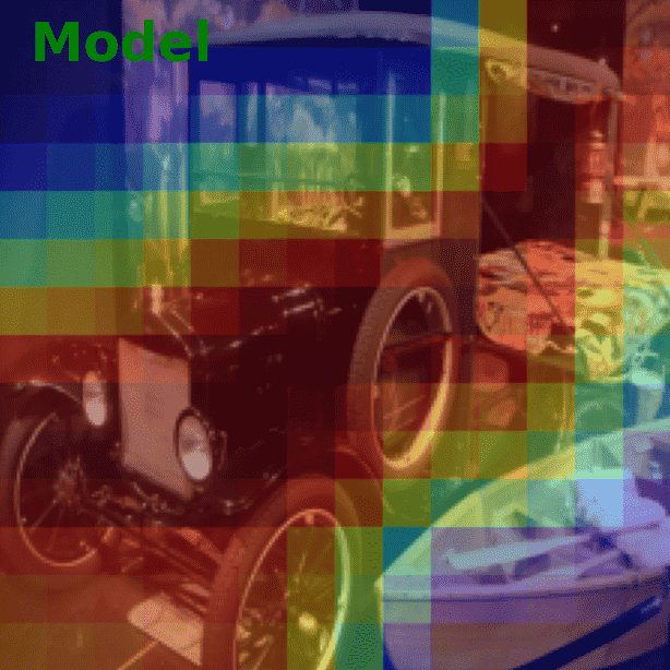
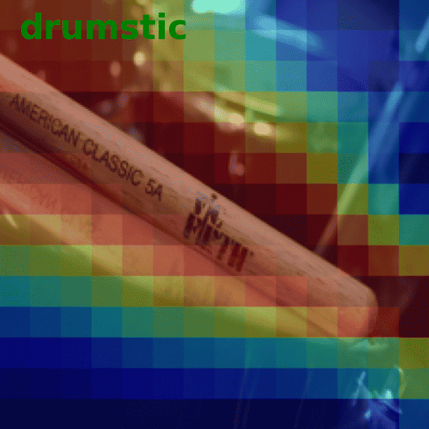
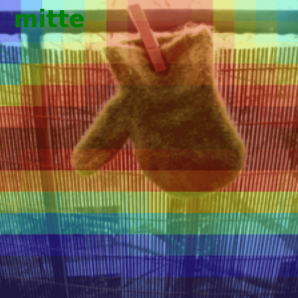
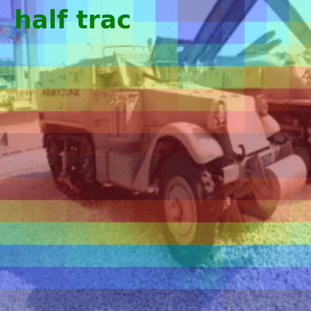
Figure 12: Explanation heatmaps of ViT-Base on the ImageNet dataset.

References

- [1] Marco Ancona, Enea Ceolini, Cengiz Öztireli, and Markus Gross. Towards better understanding of gradient-based attribution methods for deep neural networks. arXiv preprint arXiv:1711.06104, 2017.
- [2] Chia-Yuan Chang, Jiayi Yuan, Sirui Ding, Qiaoyu Tan, Kai Zhang, Xiaoqian Jiang, Xia Hu, and Na Zou. Towards fair patient-trial matching via patient-criterion level fairness constraint. arXiv preprint arXiv:2303.13790, 2023.
- [3] Hanjie Chen, Faeze Brahman, Xiang Ren, Yangfeng Ji, Yejin Choi, and Swabha Swayamdipta. Rev: information-theoretic evaluation of free-text rationales. arXiv preprint arXiv:2210.04982, 2022.
- [4] Lu Chen, Siyu Lou, Keyan Zhang, Jin Huang, and Quanshi Zhang. Harsanyinet: Computing accurate shapley values in a single forward propagation. arXiv preprint arXiv:2304.01811, 2023.
- [5] Ting Chen, Simon Kornblith, Mohammad Norouzi, and Geoffrey Hinton. A simple framework for contrastive learning of visual representations. In International conference on machine learning, pages 1597–1607. PMLR, 2020.
- [6] Sasank Chilamkurthy. Transfer learning for computer vision tutorial. PyTorch Tutorials, 2017.
- [7] Yu-Neng Chuang, Guanchu Wang, Fan Yang, Zirui Liu, Xuanting Cai, Mengnan Du, and Xia Hu. Efficient xai techniques: A taxonomic survey. arXiv preprint arXiv:2302.03225, 2023.
- [8] Yu-Neng Chuang, Guanchu Wang, Fan Yang, Quan Zhou, Pushkar Tripathi, Xuanting Cai, and Xia Hu. Cortx: Contrastive framework for real-time explanation. arXiv preprint arXiv:2303.02794, 2023.
- [9] Ian Covert, Chanwoo Kim, and Su-In Lee. Learning to estimate shapley values with vision transformers. arXiv preprint arXiv:2206.05282, 2022.
- [10] Jia Deng, Wei Dong, Richard Socher, Li-Jia Li, Kai Li, and Li Fei-Fei. Imagenet: A large-scale hierarchical image database. In 2009 IEEE conference on computer vision and pattern recognition, pages 248–255. Ieee, 2009.
- [11] Alexey Dosovitskiy, Lucas Beyer, Alexander Kolesnikov, Dirk Weissenborn, Xiaohua Zhai, Thomas Unterthiner, Mostafa Dehghani, Matthias Minderer, Georg Heigold, Sylvain Gelly, et al. An image is worth 16x16 words: Transformers for image recognition at scale. arXiv preprint arXiv:2010.11929, 2020.
- [12] Mengnan Du, Ninghao Liu, and Xia Hu. Techniques for interpretable machine learning. Communications of the ACM, 63(1):68–77, 2019.
- [13] Jeremy Elson, John (JD) Douceur, Jon Howell, and Jared Saul. Asirra: A captcha that exploits interest-aligned manual image categorization. In Proceedings of 14th ACM Conference on Computer and Communications Security (CCS). Association for Computing Machinery, Inc., October 2007.
- [14] Kawin Ethayarajh, Yejin Choi, and Swabha Swayamdipta. Understanding dataset difficulty with v-usable information. pages 5988–6008, 2022.
- [15] Luciano Floridi. Establishing the rules for building trustworthy ai. Nature Machine Intelligence, 1(6):261–262, 2019.
- [16] Bryce Goodman and Seth Flaxman. European union regulations on algorithmic decision-making and a “right to explanation”. AI magazine, 38(3):50–57, 2017.
- [17] Kaiming He, Xinlei Chen, Saining Xie, Yanghao Li, Piotr Dollár, and Ross Girshick. Masked autoencoders are scalable vision learners. In Proceedings of the IEEE/CVF conference on computer vision and pattern recognition, pages 16000–16009, 2022.
- [18] Kaiming He, Haoqi Fan, Yuxin Wu, Saining Xie, and Ross Girshick. Momentum contrast for unsupervised visual representation learning. In Proceedings of the IEEE/CVF conference on computer vision and pattern recognition, pages 9729–9738, 2020.
- [19] John Hewitt, Kawin Ethayarajh, Percy Liang, and Christopher D Manning. Conditional probing: measuring usable information beyond a baseline. arXiv preprint arXiv:2109.09234, 2021.
- [20] Jeremy Howard. Imagenette: A smaller subset of 10 easily classified classes from imagenet, March 2019.
- [21] Neil Jethani, Mukund Sudarshan, Ian Connick Covert, Su-In Lee, and Rajesh Ranganath. Fastshap: Real-time shapley value estimation. In International Conference on Learning Representations, 2021.
- [22] Alexander Kirillov, Eric Mintun, Nikhila Ravi, Hanzi Mao, Chloe Rolland, Laura Gustafson, Tete Xiao, Spencer Whitehead, Alexander C Berg, Wan-Yen Lo, et al. Segment anything. arXiv preprint arXiv:2304.02643, 2023.
- [23] Narine Kokhlikyan, Vivek Miglani, Miguel Martin, Edward Wang, Bilal Alsallakh, Jonathan Reynolds, Alexander Melnikov, Natalia Kliushkina, Carlos Araya, Siqi Yan, et al. Captum: A unified and generic model interpretability library for pytorch. arXiv preprint arXiv:2009.07896, 2020.
- [24] Alex Krizhevsky, Geoffrey Hinton, et al. Learning multiple layers of features from tiny images. 2009.
- [25] Yang Liu, Sujay Khandagale, Colin White, and Willie Neiswanger. Synthetic benchmarks for scientific research in explainable machine learning. 2021.
- [26] Ze Liu, Yutong Lin, Yue Cao, Han Hu, Yixuan Wei, Zheng Zhang, Stephen Lin, and Baining Guo. Swin transformer: Hierarchical vision transformer using shifted windows. In Proceedings of the IEEE/CVF international conference on computer vision, pages 10012–10022, 2021.
- [27] Scott M Lundberg and Su-In Lee. A unified approach to interpreting model predictions. Advances in neural information processing systems, 30, 2017.
- [28] Rory Mitchell, Joshua Cooper, Eibe Frank, and Geoffrey Holmes. Sampling permutations for shapley value estimation. The Journal of Machine Learning Research, 23(1):2082–2127, 2022.
- [29] Vitali Petsiuk, Abir Das, and Kate Saenko. Rise: Randomized input sampling for explanation of black-box models. arXiv preprint arXiv:1806.07421, 2018.
- [30] Marco Tulio Ribeiro, Sameer Singh, and Carlos Guestrin. ” why should i trust you?” explaining the predictions of any classifier. In Proceedings of the 22nd ACM SIGKDD international conference on knowledge discovery and data mining, pages 1135–1144, 2016.
- [31] Yao Rong, Guanchu Wang, Qizhang Feng, Ninghao Liu, Zirui Liu, Enkelejda Kasneci, and Xia Hu. Efficient gnn explanation via learning removal-based attribution. arXiv preprint arXiv:2306.05760, 2023.
- [32] Ramprasaath R Selvaraju, Michael Cogswell, Abhishek Das, Ramakrishna Vedantam, Devi Parikh, and Dhruv Batra. Grad-cam: Visual explanations from deep networks via gradient-based localization. In Proceedings of the IEEE international conference on computer vision, pages 618–626, 2017.
- [33] Emily Steel and Julia Angwin. On the web’s cutting edge, anonymity in name only. The Wall Street Journal, 4, 2010.
- [34] Ao Sun, Pingchuan Ma, Yuanyuan Yuan, and Shuai Wang. Explain any concept: Segment anything meets concept-based explanation. arXiv preprint arXiv:2305.10289, 2023.
- [35] Yanpeng Sun, Qiang Chen, Xiangyu He, Jian Wang, Haocheng Feng, Junyu Han, Errui Ding, Jian Cheng, Zechao Li, and Jingdong Wang. Singular value fine-tuning: Few-shot segmentation requires few-parameters fine-tuning. Advances in Neural Information Processing Systems, 35:37484–37496, 2022.
- [36] Mukund Sundararajan, Ankur Taly, and Qiqi Yan. Axiomatic attribution for deep networks. In International conference on machine learning, pages 3319–3328. PMLR, 2017.
- [37] Hugo Touvron, Matthieu Cord, Matthijs Douze, Francisco Massa, Alexandre Sablayrolles, and Hervé Jégou. Training data-efficient image transformers & distillation through attention. In International conference on machine learning, pages 10347–10357. PMLR, 2021.
- [38] Guanchu Wang, Yu-Neng Chuang, Mengnan Du, Fan Yang, Quan Zhou, Pushkar Tripathi, Xuanting Cai, and Xia Hu. Accelerating shapley explanation via contributive cooperator selection. arXiv preprint arXiv:2206.08529, 2022.
- [39] Thomas Wolf, Lysandre Debut, Victor Sanh, Julien Chaumond, Clement Delangue, Anthony Moi, Pierric Cistac, Tim Rault, Rémi Louf, Morgan Funtowicz, et al. Transformers: State-of-the-art natural language processing. In Proceedings of the 2020 conference on empirical methods in natural language processing: system demonstrations, pages 38–45, 2020.
- [40] Thomas Wolf, Lysandre Debut, Victor Sanh, Julien Chaumond, Clement Delangue, Anthony Moi, Pierric Cistac, Tim Rault, Rémi Louf, Morgan Funtowicz, Joe Davison, Sam Shleifer, Patrick von Platen, Clara Ma, Yacine Jernite, Julien Plu, Canwen Xu, Teven Le Scao, Sylvain Gugger, Mariama Drame, Quentin Lhoest, and Alexander M. Rush. Transformers: State-of-the-art natural language processing. In Proceedings of the 2020 Conference on Empirical Methods in Natural Language Processing: System Demonstrations, pages 38–45, Online, October 2020. Association for Computational Linguistics.
- [41] Yilun Xu, Shengjia Zhao, Jiaming Song, Russell Stewart, and Stefano Ermon. A theory of usable information under computational constraints. arXiv preprint arXiv:2002.10689, 2020.
- [42] Fan Yang, Ninghao Liu, Suhang Wang, and Xia Hu. Towards interpretation of recommender systems with sorted explanation paths. In 2018 IEEE International Conference on Data Mining (ICDM), pages 667–676. IEEE, 2018.
- [43] Zhou Yang, Ninghao Liu, Xia Ben Hu, and Fang Jin. Tutorial on deep learning interpretation: A data perspective. In Proceedings of the 31st ACM International Conference on Information & Knowledge Management, pages 5156–5159, 2022.
- [44] Anna Zimdars. Fairness and undergraduate admission: a qualitative exploration of admissions choices at the university of oxford. Oxford Review of Education, 36(3):307–323, 2010.