Optimal Decision Tree with Noisy Outcomes

Abstract

In pool-based active learning, the learner is given an unlabeled data set and aims to efficiently learn the unknown hypothesis by querying the labels of the data points. This can be formulated as the classical Optimal Decision Tree (ODT) problem: Given a set of tests, a set of hypotheses, and an outcome for each pair of test and hypothesis, our objective is to find a low-cost testing procedure (i.e., decision tree) that identifies the true hypothesis. This optimization problem has been extensively studied under the assumption that each test generates a deterministic outcome. However, in numerous applications, for example, clinical trials, the outcomes may be uncertain, which renders the ideas from the deterministic setting invalid. In this work, we study a fundamental variant of the ODT problem in which some test outcomes are noisy, even in the more general case where the noise is persistent, i.e., repeating a test gives the same noisy output. Our approximation algorithms provide guarantees that are nearly best possible and hold for the general case of a large number of noisy outcomes per test or per hypothesis where the performance degrades continuously with this number. We numerically evaluated our algorithms for identifying toxic chemicals and learning linear classifiers, and observed that our algorithms have costs very close to the information-theoretic minimum.

Keywords: approximation algorithms, active learning, optimal decision tree, submodular functions, stochastic set cover

1 Introduction

In the Optimal Decision Tree (ODT) problem, our objective is to identify an unknown true hypothesis drawn from a known prior distribution over a given set of hypotheses. To collect information on the true hypothesis, we are also given a set of tests. Upon selection, a test produces a binary (i.e., positive or negative) outcome that depends on the true hypothesis, and a certain cost is incurred. Finally, we are given a binary matrix that documents the outcome of every pair of test and hypothesis. The goal is to find a low-cost testing procedure (i.e., decision tree) that always identifies the true hypothesis.

This fundamental problem encapsulates many real-world challenges wherein the learner aims to interactively gather information to identify the unknown ground truth. For example, in medical diagnosis, a doctor must diagnose a patient’s unknown disease by performing a low-cost sequence of medical tests, chosen from a set of available tests (Loveland, 1985). As another example, in active learning (e.g., Dasgupta 2005), the learner is given a set of unlabeled data points and aims to find a correct binary classifier by efficiently querying the labels of the data points. Other applications include entity identification in databases (Chakaravarthy et al. 2011) and experimental design to choose the most accurate theory among competing candidates (Golovin et al. 2010).

The ODT problem has been extensively studied under the assumption that each test generates a deterministic outcome. However, this assumption is unrealistic in many applications. For example, in clinical trials, the results of the same medical test may vary among individuals due to genetic differences, despite the fact that they share the same underlying disease. Similarly, in online A/B experiments, users’ reactions to a particular treatment (“test”) may vary within the same user group (“hypothesis”) due to personal preferences.

Despite the considerable literature on the ODT problem, the fundamental problem of ODT with noisy outcomes is not yet adequately understood, especially from the perspective of approximation algorithms. Previous work incorporating noise (e.g., Golovin et al. 2010) was restricted to settings with very few noisy outcomes. One of the central technical challenges in the presence of noise is that each hypothesis can potentially follow one of an exponential (in the level of uncertainty) number of trajectories. This leads to an unfavorable approximation ratio if the noise-free analysis is applied directly.

Against this backdrop, we embark on a comprehensive study of the fundamental problem of Optimal Decision Tree with Noise (ODTN) in full generality and design novel approximation algorithms with provable guarantees. Essentially, we generalize the ODT problem to the setting where the test-hypothesis matrix may contain some independently random entries. The positions of these entries are known but their values can only be revealed when the corresponding test is performed.

Adding to the challenge, we consider the persistent noise model, where repeating the same test always produces the same outcome. This model is (a) more general and (b) more challenging than the independent noise model, which is more common in the literature on active learning and ODT. In fact, to see (a), we can reduce the independent noise model to the persistent noise model by creating sufficiently many copies of each test. To see (b), note that in the independent noise model, we can “denoise” by repeating a test many times and reducing the problem to a deterministic one. However, this approach obviously fails under persistent noise.

	what to choose	what is unknown	what to observe
AL	unlabeled data	classifier	label
ODT	test	hypothesis	outcome
ASR	element	target function	response

Table 1: One stone, three birds: Analogous terminologies in active learning (AL), optimal decision tree (ODT), and adaptive submodular ranking (ASR).

Beyond the ODTN problem, our results are valid in a substantially more general setting, called Adaptive Submodular Ranking with Noise (ASRN): Given a set of elements, we need to construct a subset of elements sequentially to cover an unknown target function, which comes from a given family of submodular functions. When an element is selected, we not only increase the value of the target function but also receive a random response that helps further localize the target function in the given family. Therefore, we face a learning-versus-earning trade-off: An intelligent algorithm must consider both the coverage and the information gain when selecting the next element. The goal is to minimize the cover time of the target function, i.e., the expected number of elements selected until the value of the target function reaches a prescribed threshold.

The ASRN problem generalizes the ODTN problem. To see this, note that since the output must be correct with probability $1$, we need to eliminate all but one hypothesis. This motivates us to consider a set function for each hypothesis, whose value is proportional to the number of other hypotheses eliminated. Intuitively, this function is submodular: The elimination power of the same test diminishes as we select more tests. Our objective is to cover the submodular function of the true hypothesis, which is unknown initially but can be “learned” as we observe more test outcomes. To help the reader see the connection, we list and compare analogous concepts in these problems in Table 1.

In the absence of noisy outcomes, this problem has been studied in both non-adaptive (Azar and Gamzu, 2011) and adaptive (Navidi et al., 2020) settings. In addition to the ODT problem, this submodular setting captures a number of applications such as Multiple-intent Search Ranking (Azar et al., 2009), Decision Region Determination (Javdani et al., 2014) and Correlated Knapsack Cover (Navidi et al., 2020). Our work is the first to handle noisy outcomes in all of these applications in a unified manner.

1.1 Contributions

Our results can be categorized into the following four parts.

1. Non-adaptive Setting. We first consider the non-adaptive version of the ASRN problem, dubbed Submodular Function Ranking with Noise (SFRN). We obtain a polynomial-time algorithm with cost $O(\log\frac{1}{\varepsilon})$ times the optimum; see Theorem 14. Here, $\varepsilon>0$ is the separability of the family of submodular functions, formally defined in Section 2. This result is significant because of the following aspects.

   1. Implications for the ODTN Problem: The above implies an $O(\log m)$-approximation for the non-adaptive ODTN problem where $m$ is the number of hypotheses. This is best possible assuming ${\rm P}\neq{\rm NP}$, due to the renowned APX-hardness result for the Set Cover problem; see Theorem 4.4 in Feige 1998.

   2. Optimality: Unless ${\rm P}={\rm NP}$, there is no polynomial-time $o(\log\frac{1}{\varepsilon})$-approximation algorithm (even without noise); see Theorem 3.1 in Azar and Gamzu 2011.

2. Adaptive Setting with Low Noise. We present an algorithm whose performance guarantee degrades with the noise level. Specifically, we introduce the notions of row uncertainty $r$ and column uncertainty $c$ (formally defined in Section 5), and present an $O(\min\{c,r\}+\log\frac{m}{\varepsilon})$-approximation algorithm for the ASRN problem where $m$ is the number of submodular functions; see Theorem 19. In the noiseless case, i.e., $c=r=0$, our result matches the known bound (Theorem 1 in Navidi et al. 2020) for the special case without noise. Our result is significant in the following respects.

   1. Implications for the ODTN Problem: By setting $\varepsilon=\frac{1}{m}$, we immediately obtain an $O(\min\{c,r\}+\log m)$ approximation for the (adaptive) ODTN problem. In this context, $c$ (resp. $r$) is the maximum number of noisy outcomes in each column (resp. row) of the test-hypothesis matrix.

   2. Optimality Under Low Noise Level: If the number of noisy outcomes in each row or column is $O(\log\frac{m}{\varepsilon})$, the approximation ratio becomes $O(\log\frac{m}{\varepsilon})$, which is best possible due to Theorem 4.1 in Chakaravarthy et al. 2011.

   3. Improved Approximation for the ODTN Problem: Golovin et al. (2010) obtained an $O(\log^{2}\frac{1}{p_{\rm min}})$-approximation that is polynomial-time only when $c=O(\log m)$, where $p_{\rm min}\leq\frac{1}{m}$ is the minimum probability mass of any hypothesis. Our result improves the above by a logarithmic factor and is polynomial-time regardless of $c,r$.

3. Adaptive Setting with High Noise. So far we have focused on the case with few uncertain entries in the test-hypothesis matrix. Now, we consider the other extreme, where this matrix has few deterministic entries. At first sight, considering the increased level of noise, the problem appears considerably more challenging. Surprisingly, we obtain a logarithmic approximation by combining the following components.

   1. Sparsity of the Instance: An ODTN instance is $\alpha$-sparse for some $\alpha\in[0,1]$ if each test has $O(m^{\alpha})$ deterministic outcomes. The lower $\alpha$, the more challenging it is to identify the true hypothesis. We quantify this relation by showing that the optimum is $\Omega(m^{1-\alpha})$; see Proposition 21.

   2. Lower Bound via Stochastic Set Cover: As the key technical novelty, we relate the ODTN problem to the Stochastic Set Cover (SSC) problem by “charging” the cost to a family of SSC instances. For each hypothesis $i$, we associate an SSC instance and show that its optimum, denoted ${\rm OPT}_{{\rm SSC}(i)}$, is a lower bound on the cost of any algorithm attributed to $i$. We then show that the optimum is at least the sum of ${\rm OPT}_{{\rm SSC}(i)}$’s, weighted by the prior probabilities.

   3. A Novel Greedy Algorithm: Motivated by the above observation, we present a hybrid algorithm that integrates (i) the greedy algorithm for the SSC problem and (ii) a brute-force subroutine that checks whether one of the hypotheses with the highest posterior probability is the true hypothesis; see Algorithm 4. This algorithm has a low cost since (i) the greedy SSC algorithm is an $O(\log m)$-approximation, and (ii) the brute-force subroutine enumerates only a small number of hypotheses.

   4. Approximation for $\alpha$-Sparse Instances: Building on (b) and (c), we show that the above algorithm has cost $O(m^{\alpha}+\log m\cdot{\rm OPT})$ for any $\alpha$-sparse instance; see Theorem 26. When $\alpha\leq\frac{1}{2}$, we have ${\rm OPT}=\Omega(m^{\alpha})$ due to (a), and we obtain an $O(\log m)$-approximation.

4. Comprehensive Numerical Experiments. We tested our algorithms on both a synthetic and a real data set arising from toxic chemical identification. We compared the empirical performance guarantee of our algorithms to an information-theoretic lower bound. The cost of the solution returned by our non-adaptive algorithm is typically within 50% of this lower bound, and typically within 20% for the adaptive algorithm, demonstrating the effective practical performance of our algorithms.

1.2 Related Work

The ODT problem has been extensively studied for several decades; see Garey and Graham 1974; Hyafil and Rivest 1976/77; Loveland 1985; Arkin et al. 1998; Kosaraju et al. 1999; Adler and Heeringa 2008; Chakaravarthy et al. 2009; Gupta et al. 2017; Li et al. 2020. The state-of-the-art result is an $O(\log m)$-approximation (Gupta et al., 2017), for instances with arbitrary probability distribution and costs. On the other hand, Chakaravarthy et al. (2011) showed that ODT cannot be approximated to a factor better than $O(\log m)$ unless P=NP.

The application of ODT to Bayesian active learning was formalized in Dasgupta 2005. There are also several results on the statistical complexity of active learning; see, e.g., Balcan et al. 2006; Hanneke 2007; Nowak 2009. There are two main differences from these works from ours. First, they focus on proving sample complexity bounds for structured hypothesis classes, such as threshold functions or linear classifiers. Secondly, these works primarily focus on analyzing the sample complexity, rather than comparing the cost with the optimal algorithm. On the contrary, we consider arbitrary (finite) hypothesis classes and obtain computationally efficient policies with provable approximation bounds relative to the optimal (instance-specific) policy. This approach is similar to that of Dasgupta 2005; Guillory and Bilmes 2009; Golovin and Krause 2011; Golovin et al. 2010; Cicalese et al. 2014; Javdani et al. 2014.

The noisy ODT problem was studied previously in Golovin et al. 2010. Using a connection to adaptive submodularity, Golovin and Krause (2011) obtained an $O(\log^{2}\frac{1}{p_{\rm min}})$-approximation algorithm for noisy ODT in the presence of very few noisy outcomes, where $p_{\rm min}\leq\frac{1}{m}$ is the minimum probability of any hypothesis. In particular, the running time of the algorithm in Golovin et al. 2010 is exponential in the number of noisy outcomes per hypothesis. As noted earlier, our result improves both the running time (it is now polynomial for any number of noisy outcomes) and the approximation ratio. We note that an $O(\log m)$ approximation ratio (still only for very sparse noise) follows from work on the “equivalence class determination” problem by Cicalese et al. (2014). For this setting, our result is also an $O(\log m)$ approximation, but our algorithm is simpler. More importantly, ours is the first result that can handle any number of noisy outcomes.

Other variants of noisy ODT have also been considered, where the goal is to identify the correct hypothesis with at least some target probability (Naghshvar et al., 2012; Bellala et al., 2011; Chen et al., 2017). Chen et al. (2017) provided a bi-criteria approximation in which the algorithm has a higher error probability than the optimal policy. Our setting is different because we require zero probability of error. Many results for ODT (including some of ours) rely on certain submodularity properties. We briefly survey some background results. In the basic Submodular Cover problem, we are given a set of elements and a submodular function $f$. The goal is to use the minimal number of elements to increase the value of $f$ to reach a certain threshold. Wolsey (1982) first considered this problem and proved that the natural greedy algorithm is a $(1+\ln\frac{1}{\varepsilon})$-approximation, where $\varepsilon$ is the minimal positive marginal increment of the function. As a natural generalization, in the Submodular Function Ranking problem we are given multiple submodular functions and aim to sequentially select elements so as to minimize the total cover time of these functions. Azar and Gamzu (2011) proposed a best-possible $O(\log\frac{1}{\epsilon})$-approximation algorithm for this problem, and Im et al. (2016) extended this result to also handle arbitrary costs. More recently, Navidi et al. (2020) studied an adaptive version of the submodular ranking problem and presented a best-possible $O(\log m/\varepsilon)$-approximation where $m$ is the number of functions.

Finally, we note that there is also work considering the worst-case (instead of average case) cost in ODT and active learning; see, e.g., Moshkov 2010; Saettler et al. 2017; Guillory and Bilmes 2010, 2011. These results are incomparable to ours because we are interested in the average cost. Moreover, the analysis of average cost is, in general, more intricate than that of the worst-case cost.

2 Preliminaries

In the problem of Optimal Decision Tree with Noise (ODTN), we are given a set of $m$ possible hypotheses with a prior probability distribution $\{\pi_{i}\}_{i=1}^{m}$, from which an unknown true hypothesis $\bar{i}$ is drawn. There is also a set $\mathcal{T}$ of $n$ binary tests. Each test $T\in\mathcal{T}$ is a mapping $T:[m]\rightarrow\{+1,-1,\star\}$. When this test is performed, we will observe an outcome $T(\bar{i})$ if $T(\bar{i})\neq\star$, and observe $+,-$ with probability $\frac{1}{2}$ if $T(\bar{i})=\star$. We assume that the random outcomes are independent, conditioned on the true hypothesis.

Alternatively, we can view an instance as a matrix $M\in\{+1,-1,\star\}^{n\times m}$, where each $\star$-entry is independently drawn from $+1$ and $-1$ uniformly. We emphasize that we only know the positions of the $\star$ entries but not their realized binary values, which can only be revealed when the corresponding test is selected.

We aim to identify $\bar{i}$ by iteratively eliminating hypotheses. Suppose we select a test $T$ and observe an outcome $O\in\{\pm 1\}$. Then, we can rule out the hypotheses $i\in[m]$ with $T(i)=-O$. We emphasize that we can not rule out hypotheses $h$ with $T(h)=\star$. In fact, if $h$ is the true hypothesis, then there is still non-zero probability that we will observe $O$ when $T$ is selected.

We consider the persistent noise model. That is, repeating a test $T$ with $\bar{i}\in T^{*}$ always produces the same outcome. This model is (a) more general and (b) more challenging than the independent noise model, which is more common in the literature on active learning and ODT. In fact, to see (a), we can reduce the independent noise model to the persistent noise model by creating sufficiently many copies of each test. To see (b), note that in the independent noise model, we can “denoise” by repeating a test many times and reducing the problem to a deterministic one. However, this approach fails under persistent noise.

We require that the output be correct with probability $1$. To ensure that this is feasible, we assume that the true hypothesis $\bar{i}$ can be uniquely identified by performing all tests, regardless of the outcomes of $\star$-tests, i.e., tests $T$ where $T(\bar{i})=\star$.

Assumption 1 (Identifiability).

For any hypotheses $i,j\in[m]$, there exists a test $T$ such that $T(i)\neq T(j)$ and $T(i),T(j)\in\{+1,-1\}$.

Many of our results still hold (with possibly weaker guarantees) without the identifiability assumption; see Appendix 7. Our goal is to minimize the expected number of tests performed. We formally define the cost when we introduce the more general problem of ASRN in Section 3.

3 Submodular Function Ranking and Its Variants

Many of our results for the ODTN problem are obtained as corollaries of a more general problem, Adaptive Submodular Ranking with Noise (ASRN). To define this problem, we first review the basic versions. In Section 3.1, we introduce the Submodular Function Ranking (SFR) problem (Azar and Gamzu, 2011), where elements are selected non-adaptively to cover a family of submodular functions. Then, in Section 3.2, we review the adaptive version of SFR, called the Adaptive Submodular Ranking (ASR) problem (Navidi et al., 2020), where the elements are selected to cover an unknown target submodular function, adaptively based on observed information on the target function. Finally, in Section 3.3, we dive into full generality by introducing the problem of Adaptive Submodular Ranking with Noise (ASRN), which generalizes both the ASR and ODTN problems.

3.1 Submodular Function Ranking, Noiseless Case

Let us begin with the simplest setting and gradually add components in the next two subsections. Azar and Gamzu (2011) introduced the following Submodular Function Ranking (SFR) problem. We are given a ground set of elements $[n]:=\{1,...,n\}$ and a collection of monotone submodular functions $\{f_{1},...,f_{m}\}$ where $f_{i}:2^{[n]}\rightarrow[0,1]$ satisfies $f_{i}(\emptyset)=0$ and $f_{i}([n])=1$ for all $i\in[m]$. It is without loss of generality (w.l.o.g.) to assume that the range is $[0,1]$, since any bounded function can be normalized to take values in $[0,1]$. Each $i\in[m]$ is called a scenario. An unknown target scenario is drawn from a known distribution $\{\pi_{i}\}$ over $[m]$.

Note that in this problem, we are not able to “learn” the target function based on any observable information. Therefore, a decision rule can be formulated as a permutation of elements. For a fixed permutation $\sigma$, we define the cover time of a scenario $i$ as the first time $f_{i}$ reaches the value $1$ if we select elements one by one according to $\sigma$. The objective in the SFR problem is to find a permutation $\sigma$ of $[n]$ with minimal expected cover time.

Definition 1 (Cover Time and Cost).

Let $\sigma=(\sigma(1),\dots,\sigma(n))$ be any permutation of the elements and $i\in[m]$ be a scenario. Then, the cover time is defined as

$$C(i,\sigma):=\min\left\{t\ |f_{i}(\{\sigma(1),...,\sigma(t)\})=1\right\}.$$

The cost of $\sigma$ is ${\rm Cost}(\sigma):=\sum_{i\in[m]}\pi_{i}\cdot C(i,\sigma).$

Azar and Gamzu (2011) proposed a greedy algorithm that constructs a permutation of elements by iteratively selecting the next element with the highest score. This score assigns higher priority to those scenarios close to being covered. Specifically, the weight of each scenario is inversely proportional to the distance from $1$ and the current value of $f_{i}$. We will formally state this algorithm in the form of pseudo-code in Algorithm 1 after we introduced the noisy variant in the next subsection.

This algorithm has the best possible approximation ratio in terms of separability parameter $\varepsilon>0$, defined as the minimum positive marginal increment of any function.

Definition 2 (Separability).

Given a family of non-decreasing functions $\mathcal{F}$, its separability is defined as

$$\varepsilon:=\min\{f_{i}(S\cup\{e\})-f_{i}(S)>0\ |\ \forall S\subseteq[n],i\in[m],e\in[n]\}.$$

Azar and Gamzu (2011) showed the following in their Theorem 2.1.

Theorem 3 (Azar and Gamzu 2011).

There is a polynomial-time algorithm whose cost is $O(\log\frac{1}{\varepsilon})$ times the optimum for any SFR instance with separability parameter $\varepsilon>0$.

3.2 Adaptive Submodular Ranking, Noiseless Case

An instance in the Adaptive Submodular Ranking (ASR) problem is slightly more involved than in the SFR problem in the following two ways. First, for each scenario $i\in[m]$, there is a known response function $r_{i}:[n]\rightarrow\Omega$ where $\Omega$ is a finite set of responses (or outcomes, which we use interchangeably). If $i$ is the true scenario and an element $e\in[n]$ is selected, then a response $\omega=r_{i}(e)\in\Omega$ is generated and thus any scenario $j$ with $r_{j}(e)\neq\omega$ can be eliminated. Second, the domain of each submodular function is expanded to incorporate the variability of the responses: The domain for each submodular function is $2^{[n]}$ in an SFR instance, and is instead $2^{[n]\times\Omega}$ in an ASR instance. The SFR problem can be cast as a special case of the ASR problem: The reduction is immediate by setting the response set $\Omega$ to a singleton.

An adaptive policy (or decision tree) constructs a sequence of elements incrementally and adaptively, based on the responses of the previous elements. A policy is simply a function that maps the current state, i.e., elements selected so far and their responses, to an element that will be selected next. We formalize this concept below.

Definition 4 (Adaptive Policy).

The state is a tuple $(E,O)$ where $E\subseteq[n]$ and $O\in\Omega^{E}$. An adaptive policy is a mapping $\Phi:2^{[n]\times\Omega}\rightarrow[n]$.

Similarly to the non-adaptive setting, we aim to minimize the expected cover time. Let $\Phi$ be an adaptive policy. Observe that, conditional on any true scenario $i\in[n]$, the sequence of elements selected is uniquely determined by $\Phi$. In fact, this sequence can be specified inductively and explicitly as follows. Suppose that elements $e_{1},\dots,e_{k}$ have been selected in the first $k$ iterations. Then, the responses are $r_{i}(e_{1}),\dots,r_{i}(e_{k})$. By the definition of $\Phi,$ the next element selected would be $e_{k+1}:=\Phi(\{(e_{t},r_{i}(e_{t})):t=1,\dots,k\})$. We denote this sequence by $\sigma_{i,\Phi}$ and define the cover time as follows.

Definition 5 (Cover Time, Adaptive Setting).

Let $\Phi$ be a policy and $i\in[m]$ be a scenario. Suppose $e_{1},\dots,e_{n}$ is the (deterministic) sequence of elements selected by $\Phi$ if $i$ is the true scenario. The cover time of $i$ is then defined as

$$C(i,\Phi):=\min\{k\mid f_{i}(\{(e_{t},r_{i}(e_{t})):t\in[k]\})=1\}.$$

The expected cover time is ${\rm ECT}(\Phi):=\sum_{i\in[m]}\pi_{i}\cdot C(i,\Phi).$

The objective of the ASR problem is to find an adaptive policy $\Phi$ with minimal expected cover time. Navidi et al. (2020) showed a best-possible approximation algorithm (see their Theorem 1) that we will apply in Section 5.

Theorem 6 (Navidi et al. 2020).

There is a polynomial-time algorithm whose cost is $O(\log\frac{m}{\epsilon})$ times the optimum for any ASR instance with separability parameter $\varepsilon>0$.

Note that the ASR problem is a generalization of the (noiseless) ODT problem. In fact, for any hypothesis $i$ in the ODT problem, we can define a submodular function $f_{i}$ that maps a subset of tests to the number of other hypotheses eliminated by these tests, if $i$ is the true hypothesis.

Analogously, we next introduce a noisy version of the ASR problem and show that it generalizes the ODTN problem.

3.3 Adaptive Submodular Ranking with Noise

We now formally define the problem of Adaptive Submodular Ranking with Noise (ASRN). An ASRN instance is almost identical to that of an ASR instance: We are given a set of $n$ elements and a set of $m$ scenarios. Each scenario $i\in[m]$ is associated with a known submodular function $f_{i}:2^{[n]\times\Omega}\rightarrow[0,1]$. We are also given a known prior distribution $(\pi_{i})$ over the scenarios.

The only difference lies in the response function: For each scenario $i$, the response function $r_{i}:[n]\rightarrow\Omega\cup\{\star\}$ can take a special value $\star$. Suppose $i\in[m]$ is the true hypothesis and $r_{i}(e)=\star$, then the response will be independently drawn from a known distribution on $\Omega$. For simplicity, we will consider uniform distribution, although our results extend to arbitrary distributions.

Although the responses are random, we can still use them to eliminate scenarios. To see this, take $\Omega=\{\pm 1\}$. Suppose $i\in[m]$ is the true hypothesis and $r_{i}(e)=\star$ for some element $e\in[n]$. When $e$ is selected, we observe $+1,-1$ with probability $1/2$. If $+1$ is observed, then we eliminate every scenario $j$ with $r_{j}(e)=-1$. Similarly, if $-1$ is observed, then we eliminate every scenario $j$ with $r_{j}(e)=+1$. In other words, a random outcome helps eliminate a random subset of scenarios.

As a key technique challenge, unlike in the deterministic case, a scenario $i\in[m]$ may follow multiple (more precisely, exponentially many in the number of $\star$’s) paths in the decision tree corresponding to policy $\Phi$. To formally define the cover time, we observe that, conditioned on the realized responses of all elements, the policy selects a deterministic sequence of elements. To formalize this idea, we need the following notion of consistent vectors.

Definition 7 (Consistency of Response Vectors).

A vector $\omega=(\omega_{e})_{e\in[n]}\in\Omega^{n}$ is consistent with a scenario $i\in[m]$ if for any element $e\in[n]$ with $r_{i}(e)\neq\star$, it holds that $r_{i}(e)=\omega_{e}$.

Using terminologies from probability theory, conditioned on the event that the true scenario is $i$, we can view $\Omega^{n}$ as the ground set (for the probability space) and $\omega$ as a “sample path”. This probability space is equipped with a uniform probability measure over all sample paths consistent with $i$. Next, we define conditional cover time as a random variable (i.e., a function defined on $\Omega^{n}$) that maps each sample path $\omega$ to the cover time conditioned on $\omega$.

Definition 8 (Conditional Cover Time).

Let $\Phi$ be an adaptive policy. Let $i\in[m]$ be a scenario and $\omega\in\Omega^{n}$ be a consistent vector. We denote by $\sigma_{i,\omega}=(\sigma_{i,\omega}(1),\dots,\sigma_{i,\omega}(n))$ the unique sequence of elements selected by $\Phi$ if $i$ is the true scenario and the responses are given by $\omega$. We write $\sigma:=\sigma_{i,\omega}$ as a shorthand and define the conditional cover time as

$$C(i,\Phi|\omega):=\min\{k\ |\ f_{i}(\{(e_{\sigma(1)},\omega_{\sigma(1)}),\dots,(e_{\sigma(k)},\omega_{\sigma(k)})\})=1\}.$$

To define the cost of a policy, we take the expectation over (i) all scenarios and (ii) all sample paths, conditional on a scenario.

Definition 9 (Cost of a Policy).

Let $\Phi$ be a policy and $\omega\in\Omega^{n}$. Let $p_{\omega|i}$ be the probability mass of $\omega$ when $i$ is the true hypothesis, and define the expected cover time of $i$ as $\mathrm{ECT}(i,\Phi):=\sum_{\omega\in\Omega^{n}}p_{\omega|i}\cdot C(i,\Phi|\omega).$ The cost of $\Phi$ is defined as

$${\rm Cost}(\Phi):=\sum_{i\in[m]}\pi_{i}\cdot\mathrm{ECT}(i,\Phi).$$

To ensure the existence of a policy with finite cost, we need an assumption analogous to the identifiability assumption for the ODTN problem (Assumption 1). We assume that for each scenario $i\in[m]$, the function $f_{i}$ can be covered w.p. $1$ if we select all elements.

Assumption 2 (Feasibility of Coverage).

For any scenario $i\in[m]$ and any $\omega\in\Omega^{n}$ consistent with $i$, we have $f_{i}(\{(e,\omega_{e}):e\in[n]\})=1$.

An important special case is where $\Omega$ is a singleton set. In this case, adaptivity does not provide any additional advantage, because we cannot observe anything informative. This setting is called Submodular Function Ranking with Noise (SFRN), and will be studied in order to obtain our results for the non-adaptive ODTN problem. We completely settle the SFRN problem in Section 4, thus setting the stage for our study of the ASRN problem in Section 5.

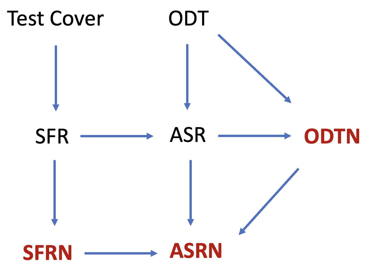
Figure 1: Connections between related problems: Edges represent (direct) reductions between problems. The test cover problem (De Bontridder et al., 2003) , which was not mentioned so far, is essentially a non-adaptive version of the ODT problem, and hence can be reduced to the SFR problem. We highlight the new problems introduced in this work in red color.

3.4 Connection to the ODTN Problem

We illustrate the connections between the problems in Figure 1. We observe that the ODTN problem can be reduced to the ASRN problem. Let us view the tests and hypotheses in the ODTN problem as elements and scenarios respectively in the ASRN problem. For any hypothesis $i\in[m]$, define its response function $r_{i}(T)=T(i)\in\Omega\cup\{\star\}$. Furthermore, for any $i\in[m]$ and any $S\subseteq\mathcal{T}\times\{\pm 1\}$, we define a submodular function

$$f_{i}(S)=\frac{1}{m-1}\cdot\left|\bigcup_{T:(T,+1)\in S}T^{-}\,\bigcup\,\bigcup_{T:(T,-1)\in S}T^{+}\right|,$$

where we recall that each test is a three-way partition $(T^{+},T^{-},T^{*})$ of $[m]$. In words, $f_{i}(S)$ is the fraction of hypotheses (other than $i$) that are incompatible with at least one outcome in $S$.

It is easy to see that each function $f_{i}:2^{[n]\times\Omega}\rightarrow[0,1]$ is monotone and submodular. Furthermore, the separability parameter $\varepsilon=\frac{1}{m-1}$. More importantly, we observe that $i$ is identified if and only if the function $f_{i}$ has value $1$. The reduction follows by combining the above observations.

3.5 Expanded Scenario Set

For both non-adaptive and adaptive settings, given an ASRN instance ${\cal I}$, we will consider an equivalent ASR instance ${\cal J}$. Thus, we can apply known algorithms for the ASR problem to the ASRN setting, and immediately bound the approximation ratio.

We emphasize that this does not suggest that our results are mere straightforward extensions of the known results for the ASR problem. In fact, the instance ${\cal J}$ is exponentially large compared to the original instance ${\cal I}$, and therefore it is highly non-trivial to find an efficient implementation of the ASR-based algorithm. In fact, most of Section 4 and Section 5 is dedicated to elucidating our efficient implementation.

In this subsection, we focus on explaining how to define the equivalent ASR instance. Let $\cal I$ be a given ASRN instance with scenarios $[m]$, submodular functions $\{f_{i}(\cdot)\}$ and response functions $\{r_{i}(\cdot)\}$. In the ASR instance $\cal J=\cal J(\cal I)$, each scenario in the original instance is divided into an exponential number of expanded scenarios, each corresponding to a sample path.

Definition 10 (Expanded Scenarios).

For each $i\in[m]$, denote

$$\Omega(i) :=\{\omega\in\Omega^{n}:\omega\ {\rm is\ consistent\ with}\ i\}$$

$$=\{\omega\in\Omega^{n}\,:\,\omega_{e}=r_{i}(e){\rm\ for\ all\ }e\in[n]{\rm\ with\ }r_{i}(e)\neq\star\}.$$

An expanded scenario is a tuple $(i,\omega)$ where $\omega\in\Omega(i)$. Furthermore, we denote $H_{i}:=\{(i,\omega)\,:\,\omega\in\Omega(i)\}$ and $H:=\bigcup_{i=1}^{m}H_{i}$.

To define the prior distribution in the new instance, for a fixed scenario $i$, consider $c_{i}:=|\{e\in[n]:r_{i}(e)=\star\}|$. Since the response of any $\star$-element for $i$ is uniformly drawn from $\Omega$, each of these $|\Omega|^{c_{i}}$ possible expanded scenarios occurs with the same probability $\pi_{i,\omega}=\pi_{i}/|\Omega|^{c_{i}}$. To complete the reduction, for each $(i,\omega)\in H$, we define the response function $r_{i,\omega}:[n]\rightarrow\Omega$ where

$$r_{i,\omega}(e)=\omega_{e},\qquad\forall e\in[n],$$

and the submodular function $f_{i,\omega}:2^{[n]}\rightarrow[0,1]$ where

$$f_{i,\omega}(S)=f_{i}\left(\{(e,\omega_{e}\right)\}_{e\in S}),\qquad\forall S\subseteq[n].$$

By this definition, since $f_{i}$ is monotone and submodular on $[n]\times\Omega$, the function $f_{i,\omega}$ is also monotone and submodular on $[n]$. We will formally show the following in Appendix A.

Proposition 11 (Reduction to the Noiseless Setting).

The ASRN instance $\cal I$ is equivalent to the ASR instance $\cal J$.

We reiterate that the number of expanded scenarios can be exponential in the number of uncertain entries, and therefore we cannot directly apply the existing algorithms for the ASR problem. We explain how to circumvent this issue in Section 4 and Section 5.

4 The Non-adaptive ASRN Problem

This main result in this section is an $O(\log\frac{1}{\varepsilon})$-approximation for the SFRN problem, where we recall that $\varepsilon>0$ is the minimal marginal increment of any submodular function in the given family. As a corollary, we obtain an $O(\log\frac{1}{m})$-approximation for the non-adaptive ODTN problem where $m$ is the number of hypotheses.

4.1 The Greedy Score

Azar and Gamzu (2011) proposed a greedy algorithm for the SFR problem. We rephrase this algorithm in the context of expanded scenarios. Suppose we have selected a set $E$ of elements. We then select the next element to be the one with the highest score, which measures the additional coverage it provides when selected.

Definition 12 (Non-adaptive Greedy Score).

Let $E\subseteq[n]$ be a subset of elements. Then, for each $e\in[n]\setminus E$, we define

$$\Delta_{E}(i,\omega,e):=\begin{cases}\frac{f_{i,\omega}(\{e\}\cup E)-f_{i,\omega}(E)}{1-f_{i,\omega}(E)},&\text{if}\ f_{i,\omega}(E)<1,\\ 0,&\text{otherwise.}\end{cases}$$ (1)

Furthermore, we define the greedy score as

$$G_{E}(e):=\sum_{(i,\omega)\in H}\pi_{i,\omega}\cdot\Delta_{E}(i,\omega;e),$$ (2)

Let us understand the intuition behind the above definition. The numerator in the ratio is the increase of $f_{i,\omega}$ when $e$ is selected. The denominator measures the remaining distance from the current value to $1$, and helps prioritize the scenarios that are close to being covered. The algorithm then selects an element $e$ with the highest $G_{E}(e)$.

4.2 Estimating the Greedy Score

Since the summation in eqn.(2) has exponentially many terms, it is not clear how to compute the exact value of $G_{E}(e)$ in polynomial time. However, since $G_{E}(e)$ is the expectation of $\Delta_{E}(i,\omega;e)$ over the expanded scenarios, we can estimate it and select an approximately greediest element by sampling. The performance of this approach is guaranteed by the following result, which follows directly from the analysis in Azar and Gamzu (2011) and Im et al. (2016).

Theorem 13 (Approximate Greedy Algorithm).

Let $\sigma=(e_{1},\dots,e_{n})$ be a permutation of elements and denote $E^{t}:=(e_{1},\dots,e_{t})$ for $t\geq 1$ and $E^{0}:=\emptyset$. Suppose for each $t=0,\dots,n-1$, we have

$$G_{E^{t}}(e_{t+1})\geq\Omega(1)\cdot\max_{e^{\prime}\in[n]\backslash E^{t}}G_{E^{t}}(e^{\prime}).$$

Then,

$${\rm Cost}(\sigma)\leq O\left(\log\frac{1}{\varepsilon}\right)\cdot{\rm OPT}$$

where $\rm OPT$ denotes the optimum of the SFRN problem.

1:Initialize $E\leftarrow\emptyset$ and permutation $\sigma=\emptyset$.

2:for $t=1,\dots,n$ do

3:     $E\leftarrow\{\sigma(1),\dots,\sigma(t-1)\}$

4:     For each $e\in[n]\backslash E$, let $\overline{G_{E}}(e)$ be the empirical mean of $\Delta_{E}(i,\omega;e)$ over $N=m^{3}n^{4}\varepsilon^{-1}$ independent draws of expanded scenarios $(i,\omega)$ from the distribution $(\pi_{i,\omega})$.

5:     Let $\sigma(t)$ be the element $e\in[n]\setminus E$ that maximizes $\overline{G_{E}}(e)$.

6:Return the permutation  $\sigma$.

Algorithm 1 Non-adaptive SFRN algorithm

To find such an approximately greediest element, for a fixed element $e$, we independently sample a polynomial number of expanded scenarios from the distribution $(\pi_{i,\omega})$. We evaluate $\Delta_{E}(i,\omega,e)$ for each expanded scenario $(i,\omega)$ sampled, and compute their empirical mean. Due to standard concentration bounds, the deviation from $G_{E}(e)$, which is its expectation, is likely small. Therefore, the empirical mean can serve as a reliable estimate of the greedy score. We formally define this algorithm in Algorithm 1.

4.3 Handling Small Greedy Score

The desired $O(\log\frac{1}{\varepsilon})$-approximation would immediately follow if we could show that the estimation is always within a (multiplicative) $O(1)$ factor to the true score $G_{E}(e)$ for every element $e$. Unfortunately, this is not true. In fact, it may fail when $G_{E}(e)$ is tiny for every element $e$.

To see this, consider an i.i.d. sample $X_{1},\dots,X_{k}$ (which corresponds to $\Delta_{E}(i,\omega;E)$), each with mean $\mu>0$ (which corresponds to $G_{E}(e)$). Chernoff’s inequality states that the probability of having a large deviation decays exponentially in $k\mu$. In other words, to ensure a target level of confidence, we need the sample complexity $k$ to scale as $\Omega(1/\mu)$, which can be large when $\mu$ is small.

To overcome this, we observe that if the score is small for all elements, then the set of elements selected so far is likely to have already covered all scenarios. Therefore, the choice of the next element is barely relevant. More precisely, we show that if $\overline{G_{E}}(e)$ is less than a certain (small) threshold that scales polynomially in $n,m$ and $1/\varepsilon$, then with probability $1-n^{-\Omega(1)}$, the current set already covers all scenarios. We formalize this in Lemma 34 in Appendix B.

So far, we have explained why our algorithm (a) is efficient (in Section 4.1), (b) identifies a sufficiently greedy element until all scenarios are covered (in Section 4.3), and (c) leads to a low approximation factor (in Section 4.2). Combining the above components, we have the following main result of this section.

Theorem 14 (Approx. Algo. for SFRN).

Algorithm 1 is a $poly(\frac{1}{\varepsilon},n,m)$ time $O(\log\frac{1}{\varepsilon})$-approximation for the SFRN problem.

It should be noted that the approximation factor is best possible due to Theorem 3.1 in Azar and Gamzu 2011. Furthermore, observe that for the ODTN problem, we have $\varepsilon=\frac{1}{m-1}$, so we obtain the following.

Corollary 15 (Approx. Algo. for Non-adaptive ODTN).

Algorithm 1 gives an $O(\log m)$-approximation for the non-adaptive ODTN problem where $m$ is the number of hypotheses.

We defer all details to Appendix B.

5 The ASRN Problem with Low Noise Level

In this section, we present an adaptive algorithm whose performance depends on the uncertainty level of the instance. Informally, suppose we store the response functions $\{r_{i}(\cdot)\}_{i\in[m]}$ as a matrix whose rows and columns correspond to the elements and scenarios. Then, the column/row uncertainty is the maximum number of $\star$’s in any column/row, formally defined as follows.

Definition 16 (Column and Row Uncertainty).

Given an ASRN instance, the column uncertainty is $c:=\max_{i\in[m]}|\{e\in[n]:r_{i}(e)=\star\}|$. Similarly, the row uncertainty is $r:=\max_{e\in[n]}\{i\in[m]:r_{i}(e)=\star\}$.

The main result of this section is an $O\left(\log\frac{m}{\varepsilon}+\min\{c\log|\Omega|,r\}\right)$-approximation for the ASRN problem for instances that have column uncertainty $c$, row uncertainty $r$ and separability $\varepsilon$. This is achieved by choosing between two algorithms, each having an approximation ratio of $O(c\log|\Omega|+\log\frac{m}{\varepsilon})$ and an $O(r+\log\frac{m}{\varepsilon})$. In both algorithms, we maintain the posterior probability of each scenario based on the responses of the selected elements. We use these probabilities to calculate a score for each element, which depends on (a) the balancedness of the partition on the remaining scenarios, resulting from selecting this element, and (b) the expected number of scenarios eliminated.

Unlike the noiseless setting, in the ASRN (and ODTN) problem, each scenario can follow an exponential number of paths in the decision tree. Therefore, a naive generalization of the analysis in Navidi et al. (2020) incurs an undesirable approximation factor.

We overcome this challenge by reducing to the ASR instance ${\cal J}$ defined in Section 3.5. However, since ${\cal J}$ involves exponentially many scenarios, a naive implementation of the algorithm in Navidi et al. (2020) leads to an exponential running time. In Section 5.1 we exploit the special structure of ${\cal J}$ and devise a polynomial-time algorithm. Then, in Section 5.2, we propose a slightly different algorithm than that of Navidi et al. (2020), and show an $O(r+\log\frac{m}{\varepsilon})$ approximation ratio.

1:Initialize $E\leftarrow\emptyset,H^{\prime}\leftarrow H$.

2:while $H^{\prime}\neq\emptyset$ do

3:     For any element $e\in[n]$, let $B_{e}(H^{\prime})$ be the largest cardinality set among

$$\{({i,\omega})\in H^{\prime}:r_{i,\omega}(e)=o\}\,\qquad\forall o\in\Omega$$

4:     Define $L_{e}(H^{\prime})=H^{\prime}\setminus B_{e}(H^{\prime})$

5:     Select the element $e\in[n]\setminus E$ maximizing

$$\mathrm{Score}_{c}(e,E,H^{\prime})=\pi\big{(}{L}_{e}(H^{\prime})\big{)}\,\,+\,\,\sum\limits_{({i,\omega})\in H^{\prime},f_{{i,\omega}}(E)<1}\pi_{{i,\omega}}\cdot\frac{f_{{i,\omega}}(e\cup E)-f_{{i,\omega}}(E)}{1-f_{{i,\omega}}(E)}$$ (3)

6:     Observe response $o$ and update $H^{\prime}$ as $H^{\prime}\leftarrow\{({i,\omega})\in H^{\prime}:\omega_{e}=o\mbox{ and }f_{{i,\omega}}(E\cup e)<1\}$

7:     $E\leftarrow E\cup\{e\}$

Algorithm 2 Algorithm for ASR instance ${\cal J}$, based on Navidi et al. (2020)

5.1 An $O(c\log|\Omega|+\log\frac{m}{\varepsilon})$-Approximation Algorithm

Our first adaptive algorithm is based on the $O(\log\frac{m}{\varepsilon})$-approximation algorithm for the (noiseless) ASR problem from Navidi et al. (2020), rephrased in our notation Algorithm 2. Applying this result to the ASR instance ${\cal J}$, we obtain an $O(\log\frac{|H|}{\varepsilon})$-approximation. Note that $|H|\leq|\Omega|^{c}\cdot m$, we immediately obtain the desired guarantee on the cost.

This algorithm maintains the set $H^{\prime}\subseteq H$ of expanded scenarios that are compatible with all the observed outcomes, and iteratively selects the element with maximum score, as defined in (3). This score strikes a balance between covering the submodular functions (of the remaining scenarios) and shrinking $H^{\prime}$ (thereby reducing the uncertainty in the target scenario).

To interpret the first term in $\mathrm{Score}_{c}$, for simplicity, assume that $\Omega=\{\pm 1\}$. Upon selecting an element, $H^{\prime}$ is split into two subsets, among which $L_{e}(H^{\prime})$ is the lighter (in cardinality). Thus, this term is simply the number of expanded scenarios eliminated in the worst case (over the responses in $\Omega$). The higher this term, the more progress is made towards identifying the target (expanded) scenario. The second term is similar to the score in our non-adaptive algorithm (Algorithm 1). It involves the sum of incremental coverage over all expanded scenarios, weighted by their current coverage, with higher weights on expanded scenarios closer to being covered.

As noted above, computing the summation in $\mathrm{Score}_{c}$ naively requires exponential time. However, in Appendix C we explain how to utilize the structure of the ASRN instance ${\cal J}$ to reformulate each of the two terms in $\mathrm{Score}_{c}$ in a manageable form, enabling a polynomial-time implementation. Now we are ready to formally state the main result of this subsection.

Theorem 17 (Approx. Algo., Low Column Uncertainty).

Algorithm 2 can be implemented in polynomial time and is an $O(c\log|\Omega|+\log\frac{m}{\varepsilon})$-approximation algorithm for the ASRN problem on any instance with column uncertainty $c$.

5.2 An $O(r+\log\frac{m}{\varepsilon})$-Approximation Algorithm

In this section, we consider a slightly different score function, $\mathrm{Score}_{r}$, and obtain an $O(r+\log\frac{m}{\varepsilon})$-approximation. Recall that in Algorithm 2, upon selecting an element $e$, the remaining expanded scenarios are partitioned into at most $|\Omega|$ subsets, where the one with the lightest cardinality is denoted $L_{e}(H^{\prime})$.

In the modified score function $\mathrm{Score}_{r}$, we instead consider the partition on the original scenarios, rather than the expanded scenarios. We define the subset $S$ of the remaining original scenarios that has at least one expanded scenario remaining. If an element $e$ is selected, then $S$ is partitioned into (at most) $|\Omega|$ subsets, where the subset with the largest cardinality is denoted as $C_{e}(S)\subseteq[m]$. The set $R_{e}(H^{\prime})\subseteq H^{\prime}$ is then defined as the consistent expanded scenarios that have a different response than $C_{e}(S)$. We formally describe this score function in Algorithm 5 in Appendix D.2.

Note that $S$ can be efficiently. More generally, for each scenario $i$, we can efficiently maintain the number $n_{i}$ of expanded scenario of $i$ that is not eliminated. In fact, observe that if we select a $\star$-element $e$ for $i$, then $n_{i}$ decreases by half. Moreover, the response is incompatible with the outcome, i.e., $r_{i}(e)\neq o$, then $n_{i}$ becomes $0$.

Similarly to Algorithm 2, the main computational challenge lies in evaluating the second term, since it involves summing over exponentially many terms, but a polynomial-time implementation follows by a similar approach as outlined in Section 5.1.

The main result of this section, stated below, is proved by adapting the proof technique from Navidi et al. (2020) and formally proved in Appendix D.2.

Theorem 18 (Apxn. Algo., Low Row Uncertainty).

Algorithm 5 can be implemented in polynomial time and is an $O(r+\log\frac{m}{\varepsilon})$-approximation algorithm for the ASRN problem for any instance with row uncertainty $r$.

By selecting between Algorithm 2 and Algorithm 5 depending on whether $c\log|\Omega|>r$, we immediately obtain the following.

Theorem 19 (Meta Algo. for ASRN).

There is an adaptive $O(\min\{c\log|\Omega|,r\}+\log\frac{m}{\varepsilon})$-approximation algorithm for the ASRN problem.

In particular, this gives an $O(\min\{c\log|\Omega|,r\}+\log\frac{m}{\varepsilon})$-approximation algorithm for the ODTN problem. We also provide closed-form expressions for the scores used in Algorithm 2 and Algorithm 5 for the ODTN problem in Appendix D.1, which will be used for our experiments.

6 ODTN with Many Unknowns

Our adaptive algorithm in Section 5 has a low approximation ratio when the vast majority of entries in the test-hypothesis matrix are deterministic. In this section, we focus on the other extreme, where ODTN instance has very few deterministic outcomes.

More precisely, we quantify the noise level by its sparsity. An ODTN instance is $\alpha$-sparse if every test has $O(m^{\alpha})$ deterministic hypotheses. Our main result is a polynomial-time approximation algorithm with cost $O(m^{\alpha}+\log m\cdot{\rm OPT})$ where ${\rm OPT}$ is the optimum of the ODTN problem, whose output may be wrong with a low probability. Furthermore, we show that for any $\alpha\in[0,1]$ we have ${\rm OPT}=\Omega(m^{1-\alpha})$. Therefore, when $\alpha<\frac{1}{2}$, we obtain an $O(\log m)$-approximation for the ODTN problem. It should be noted that the cost matches the APX-hardness result (Theorem 4.1 of Chakaravarthy et al. 2011) within $O(1)$ factors. We next explain the ideas in more detail.

6.1 Stochastic Set Cover

The design and analysis of our algorithm are closely related to the problem of Stochastic Set Cover (SSC) (Liu et al. 2008; Im et al. 2016). An SSC instance consists of a ground set $[m]$ of items and a collection of random subsets $S_{1},\cdots,S_{n}$ of $[m]$. The distribution of each subset is known, but its instantiation is unknown until being selected. The goal is to minimize the expected number of sets to cover all elements in $[m]$.

A key component of our analysis is the following lower bound on the optimum of the ODTN problem, in terms of the optima of the following SSC instances. Recall that a test $T$ can be represented as a three-way partition $(T^{+},T^{-},T^{*})$ of $[m]$.

Definition 20 (Induced SSC Instances).

For any hypothesis $i\in[m]$, let $\mathrm{SSC}(i)$ denote the SSC instance with ground set $[m]\setminus\{i\}$ and $n$ random sets, given by

$$S_{T}(i)=\left\{\begin{array}[]{ll}T^{+}\mbox{ with prob. }1&\mbox{ if }i\in T^{-}\\ T^{-}\mbox{ with prob. }1&\mbox{ if }i\in T^{+}\\ T^{-}\mbox{ or }T^{+}\mbox{ with prob. $\frac{1}{2}$ each}&\mbox{ if }i\in T^{*}\end{array}\right.,\qquad\forall T\in[n].$$

To see the connection between the SSC and ODTN problem, observe that when $i$ is the target hypothesis in the ODTN instance, any feasible algorithm must identify $i$ by eliminating all other hypotheses. In the SSC terminology, we have covered all items in $[m]\backslash\{i\}$. This leads to the following lower bound.

Proposition 21 (SSC-based Lower Bound).

For any ODTN instance with optimum OPT and induced SSC instancees $\{{\rm SSC}(i)\}_{i\in[m]}$, we have

$$\mathrm{OPT}\geq\sum_{i\in[m]}\pi_{i}\cdot\mathrm{OPT}_{\mathrm{SSC}(i)}.$$

Therefore, to bound the cost of an ODTN algorithm, we only need to charge its cost to the corresponding SSC instances and apply the above inequality. The next two subsections are dedicated to constructing such an algorithm.

6.2 A Greedy SSC Algorithm

A natural greedy algorithm is known to be an $O(\log m)$-approximation (Liu et al. 2008; Im et al. 2016). As we recall, the greedy algorithm for the (deterministic) Set Cover problem iteratively selects a set that covers the largest number of new items (i.e., items that are not covered so far). Analogously, in the SSC problem, the greedy algorithm selects the set that maximizes the expected number of new items covered.

More generally, we will consider an even more general version of the greedy algorithm, dubbed $(\beta,\rho)$-greedy where $\beta,\rho>1$ are constants. This algorithm (i) is (only) required to apply the greedy rule for an $\Omega(1/\rho)$ fraction of all iterations, and (ii) selects a set whose coverage is $\Omega(1/\beta)$ that of the greediest set when it does apply the greedy rule. We formally define this algorithm (class) in Algorithm 3.

1:Initialize $\mathcal{C}\leftarrow\emptyset,U\leftarrow[m]$.$\triangleright$ Selected sets and uncovered items

2:while $U\neq\emptyset$ do

3:     for $i\notin\mathcal{C}$ do

4:         ${\rm Cov}(i;U)\leftarrow\mathbb{E}[U\cap S_{i}]$ $\triangleright$ Compute the expected coverage of $S_{i}$      

5:     Select any $i^{*}\notin\mathcal{C}$ satisfying ${\rm Cov}(i^{*};U)\geq\frac{1}{\beta}\max_{i\in\mathcal{C}}{\rm Cov}(i;U)$

6:     Observe the instantiation $\bar{S}_{i^{*}}$ of $S_{i^{*}}$

7:     $U\leftarrow U\backslash\bar{S}_{i}$ $\triangleright$ Update the uncovered items

8:     $\mathcal{C}\leftarrow\mathcal{C}\cup\{i^{*}\}$

Algorithm 3 $(\beta,\rho)$-Greedy algorithm for the SSC Problem

The following is implied by Theorem 1.1 of Im et al. 2016 and serves as the cornerstone for our analysis.

Theorem 22 (Greedy SSC Algorithm).

Any $(\beta,\rho)$-greedy algorithm with $\beta,\rho>1$ is an $O(\beta\rho\log m)$-approximation for the SSC problem.

This result inspires a simple greedy algorithm for the ODTN problem, which we describe in the next subsection and use as a strawman to motivate further algorithmic ideas.

6.3 A First Attempt: SSC-based Greedy ODTN Algorithm

Our ODTN algorithm is inspired by the following key observation. Suppose $A$ is the set of alive (i.e., not yet eliminated) hypotheses in the ODTN problem, and a test $T$ maximizes $|T^{+}\cap A|+|T^{-}\cap A|$. Then, $T$ results in good progress for all SSC instances ${\rm SSC}(i)$ with $i\in T^{*}$ simultaneously.

Lemma 23 (Greedy Is Good for Most Hypotheses).

Let $A\subseteq[m]$ and $T$ be a test such that

$$\mathbb{E}\left[|S_{T}(i)\cap(A\backslash i)|\right]=\frac{1}{2}\left(|T^{+}\cap A|+|T^{-}\cap A|\right)\geq\max_{T^{\prime}\in[n]}\frac{1}{2}\left(|(T^{+})^{\prime}\cap A|+|(T^{-})^{\prime}\cap A|\right).$$ (4)

Then, for any hypothesis $i\in T^{*}$, we have

$$\mathbb{E}\left[|S_{T}(i)\cap(A\backslash i)|\right]\,\geq\,\frac{1}{2}\cdot\max_{T^{\prime}\in[n]}\mathbb{E}\left[|S_{T^{\prime}}(i)\cap(A\backslash i)|\right].$$

It should be noted that, in general, the above does not hold for $i\notin T^{*}$. To see this, suppose a test $T$ satisfies eqn. (4) and has imbalanced deterministic sides, for example, $|T^{+}|=m^{\alpha}$ and $|T^{-}|=1$. Then, for each $i\in T^{+}$, the random set $S_{T}$ has poor coverage in the SSC instance ${\rm SSC}(i)$, since it covers only one item (w.p. $1$).

By Lemma 23, a test $T$ makes good progress for most SSC instances if (i) $T$ satisfies eqn. (4), and (ii) $i\in T^{*}$ is satisfied for most hypotheses $i$. This motivates us to consider the class of ODTN instances where (ii) is satisfied.

Definition 24 (Sparse Instance).

An ODTN instance is $\alpha$-sparse for some $\alpha\in[0,1]$ if for all tests $T\in\mathcal{T}$ we have $\max\{|T^{+}|,|T^{-}|\}\leq m^{\alpha}$.

By this definition, if an ODTN instance is $\alpha$-sparse, then most hypotheses are in $T^{*}$. Consequently, by Lemma 23, a test $T$ satisfying eqn. (4) is $2$-greedy for most (more precisely, $m-O(m^{\alpha})$) SSC instances.

This motivates the following naive greedy algorithm. Suppose $A$ is the set of consistent hypotheses. In each iteration, we select a test $T$ that maximizes $\frac{1}{2}|T^{+}\cap A|+\frac{1}{2}|T^{-}\cap A|$. Furthermore, consider the following ideal event:

For every $t\geq 1$, when we select the $t$-th test, for every hypothesis $i\in[m]$, the algorithm has selected $\Omega(t/\rho)$ tests $T$ with $i\in T^{*}$.

If this event occurs, then the naive greedy algorithm gives an $O(\log m)$-approximation. In fact, since the sequence of tests selected is $(2,\rho)$-greedy for every $i$, by Theorem 22, the expected cost conditional on $i$ being the true hypothesis is $O(\rho\log m)\cdot\mathrm{OPT}_{\mathrm{SSC}}(i)$. Taking the expectation over all hypotheses and combining with the SSC-based lower bound in Proposition  21, we deduce that the total cost is $O(\rho\cdot\log m){\rm OPT}$.

However, the ideal event may not always occur. Next, we explain how to fix this problem by intermittently enumerating a small subset of hypotheses with the highest posterior probabilities.

6.4 Last Piece of the Puzzle: the Membership Oracle

Suppose the ideal event fails, that is, up until some iteration, the sequence of tests selected is no longer $(2,\rho)$-greedy for some hypothesis $i$. To handle this issue, we modify the above greedy algorithm as follows: For each iteration $t=2^{k}$ where $k=1,2,\dots,\log m$, we consider the set $Z=Z_{k}$ of $O(m^{\alpha})$ hypotheses with the fewest $\star$-tests selected so far. Equivalently, we may maintain a posterior probability using Bayes’ rule and define $Z$ as the subset of $O(m^{\alpha})$ hypotheses with the highest posterior probabilities.

Then, we invoke a membership oracle ${\rm Member}(Z)$ to check whether the target hypothesis $\bar{i}\in Z$. If so, then the algorithm terminates and returns $\bar{i}$. Otherwise, it continues with the greedy algorithm until the next power-of-two iteration.

Specifically, the membership oracle Member$(Z)$ takes a subset $Z\subseteq[m]$ of hypotheses as input, and decides whether the target hypothesis $\bar{i}$ is in $Z$. Whenever $|Z|\geq 2$, we pick an arbitrary pair $(j,k)$ of hypotheses in $Z$ and choose a test where these two hypotheses have distinct deterministic outcomes. Such a test exists due to Assumption 1. Moreover, since each of these tests rules out at least one hypothesis, within $|Z|-1$ iterations, there is only one hypothesis left. In Appendix E.1, we explain how to verify whether this remaining scenario is the true hypothesis using $O(\log m)$ tests.

We can bound the cost of the membership oracle as follows.

Lemma 25 (Membership Oracle Has Linear Cost).

If $\bar{i}\in Z$, then $\mathrm{Member}(Z)$ declares $\bar{i}=i$ with probability $1$; otherwise, it declares $\bar{i}\notin Z$ with probability $1-O(m^{-2})$. Furthermore, the expected cost of $\mathrm{Member}(Z)$ is $O(|Z|+\log m)$.

The formal proof of the above result is deferred to Appendix E.1. At this juncture, we have introduced all relevant concepts and ideas. In the next subsection, we formally state our results.

6.5 Sparsity-dependent Approximation Algorithm

We are now ready to state the overall algorithm in Algorithm 4. In each iteration, we maintain a subset of consistent hypotheses, and iteratively compute the greediest test, as formally specified in Step 7. At each power-of-two iteration $t=2^{k}$ where $k=1,2,\dots,\log m$, we invoke the membership oracle and terminate if it declares a true hypothesis. This algorithm has the following guarantee.

1:Initialization: consistent hypotheses $A\leftarrow[m]$, weights $w_{i}\leftarrow 0$ for $i\in[m]$, iteration index $t\leftarrow 0$

2:while $|A|>1$ do

3:     if $t$ is a power of 2 then

4:         Let $Z\subseteq A$ be the subset of $2m^{\alpha}$ hypotheses with lowest $w_{i}$

5:         Invoke Member$(Z)$

6:         If a hypothesis is identified in $Z$, then Break      

7:      Select a test $T\in\mathcal{T}$ maximizing $\frac{1}{2}(|T^{+}\cap A|+|T^{-}\cap A|)$

8:     Observe outcome $o_{T}$

9:     $R\leftarrow\{i\in[m]:M_{T,i}=-o_{T}\}$ and $A\leftarrow A\backslash R$ $\triangleright$ Remove incompatible hypotheses

10:     $w_{i}\leftarrow w_{i}+1$ for each for each $i\in T^{*}$ $\triangleright$ Update the weights of the hypotheses

11:     $t\leftarrow t+1$.

Algorithm 4 Main algorithm for large number of noisy outcomes

Theorem 26 (Apxn. Algo. for Sparse Instances).

Algorithm 4 is a polynomial-time algorithm which (a) has cost $O(m^{\alpha}+\log m\cdot{\rm OPT})$ for any $\alpha$-sparse instance with $\alpha\in[0,1]$, where $\rm OPT$ is the optimum for the ODTN problem, and (b) returns the true hypothesis with probability $1-m^{-1}$.

The choice of $m^{-1}$ is not essential: To reduce the error probability, we can simply repeat the algorithm many times and perform a majority vote, i.e., return the most frequent output. Next, we argue that the first term, $m^{\alpha}$, is negligible compared to OPT when $\alpha\leq\frac{1}{2}$.

Proposition 27 (Sparsity-based Lower Bound on OPT).

For any $\alpha$-sparse instance, we have $\mathrm{OPT}=\Omega(m^{1-\alpha})$.

In particular, when $\alpha<\frac{1}{2}$ the above implies that the cost $O(m^{\alpha})$ for each call of the membership oracle is lower than OPT, and therefore the total cost incurred in the power-of-two steps is $O(\log m\cdot\mathrm{OPT})$. We therefore conclude the following.

Corollary 28 (Logarithmic-Approximation for Sparse Instances).

Algorithm 4 has cost $O(\log m\cdot{\rm OPT})$ for any ODTN instance with $\alpha\leq\frac{1}{2}$ and returns the true hypothesis with probability $1-m^{-1}$.

6.6 Analysis Outline

We outline the proof of Theorem 26 and defer the formal proof to Appendix E.

Truncated Decision Tree. Let $\mathbb{T}$ denote the decision tree corresponding to our algorithm. We only consider tests that correspond to step 7. Recall that $H$ is the set of expanded hypotheses and that any expanded hypothesis traces a unique path in $\mathbb{T}$. For any $({i,\omega})\in H$, let $P_{i,\omega}$ denote this path traced; so $|P_{i,\omega}|$ is the number of tests performed in Step 7 under $({i,\omega})$. We will work with a truncated decision tree $\overline{\mathbb{T}}$, defined below.

Fix any expanded hypothesis $({i,\omega})\in H$. For any $t\geq 1$, let $\theta_{i,\omega}(t)$ denote the fraction of the first $t$ tests in $P_{i,\omega}$ that are $\star$-tests for hypothesis $i$. Recall that $P_{i,\omega}$ only contains tests from Step 7. Let $\rho=4$ and define

$$t_{i,\omega}=\max\left\{t\in\{2^{0},2^{1},\cdots,2^{\log m}\}\,\,:\,\,\theta_{i,\omega}(t^{\prime})\geq\frac{1}{\rho}\mbox{ for all }t^{\prime}\leq t\right\}.$$ (5)

If $t_{i,\omega}>|P_{i,\omega}|$ then we simply set $t_{i,\omega}=|P_{i,\omega}|$.

Now we define the truncated decision tree $\overline{\mathbb{T}}$. By abuse of notation, we will use $\theta_{i}(t)$ and $t_{i}$ as random variables, with randomness over $\omega$. Observe that for any $({i,\omega})$, at the next power-of-two step $2^{\lceil\log t_{i}\rceil}$, which we call the truncation time, the membership oracle will be invoked. Moreover, $2^{\lceil\log t_{i}\rceil}\leq 2t_{i}$, . This motivates us to define $\overline{\mathbb{T}}$ is the subtree of $\mathbb{T}$ consisting of the first $2^{\lceil\log t_{i,\omega}\rceil}$ tests along path $P_{i,\omega}$, for each $({i,\omega})\in H$. Under this definition, the cost of Algorithm 4 clearly equals the sum of the cost the truncated tree and cost for invoking membership oracles.

Our proof proceeds by bounding the cost of Algorithm 4 at power-of-two steps and other steps. In other words, we will decompose the cost into the cost incurred by invoking the membership oracle and selecting the greedy tests. We start with the easier task of bounding the cost for the membership oracle. The oracle Member is always invoked on $|Z|=O(m^{\alpha})$ hypotheses. Using Lemma 25, the expected total number of tests due to Step 4 is $O(m^{\alpha}\log m)$. By Lemma 27, when $\alpha\leq\frac{1}{2}$, this cost is $O(\log m\cdot\mathrm{OPT})$.

The remaining part of this subsection focuses on bounding the cost of the truncated tree as $O(\log m)\cdot\mathrm{OPT}$. With this inequality, we obtain an expected cost of

$$O(\log m)\cdot(m^{\alpha}+OPT)\leq_{(\mbox{as }\alpha<\frac{1}{2})}\,O(\log m)\cdot(m^{1-\alpha}+OPT)\leq_{\big{(}\mbox{Lemma}\leavevmode\nobreak\ \ref{lem:sparse-OPT}\big{)}}O(\log m)\cdot OPT,$$

and Theorem 26 follows. At a high level, for a fixed hypothesis $i\in[m]$, we will bound the cost of the truncated tree as follows:

$$\text{\quad\quad\quad\ \ }i\text{ has low fraction of $\star$-tests at }t_{i}$$

$$\underset{Lemma\leavevmode\nobreak\ \ref{lem:markov}}{\Longrightarrow}i\text{ is among the top }O(m^{\alpha})\text{ hypotheses\ at }t_{i}$$

$$\underset{Lemma\leavevmode\nobreak\ \ref{prop:membership_oracle}}{\Longrightarrow}i\text{ is identified w.h.p. by }\mathrm{Member}(Z)\text{ at }2^{\lceil\log t_{i}\rceil}\leq 2t_{i},\text{ hence the truncated path is }(2,2)\text{-greedy}$$

$$\underset{Theorem\leavevmode\nobreak\ \ref{thm:ssc}}{\Longrightarrow}\text{ the expected cost conditional on }i\text{ is }O(\log m)\cdot\mathrm{SSC}(i)$$

and finally by summing over $i\in[m]$, it follows from Lemma 21 that the cost of the truncated tree is $O(\log m)\cdot$OPT. We formalize each step below.

Consider the first step, formally we show that if $\theta_{i}(t)<\frac{1}{4}$, then there are $O(m^{\alpha})$ hypotheses with fewer $\star$-tests than $i$. Suppose $i$ is the target hypothesis and $\theta_{i}(t)$ drops below $\frac{1}{4}$ at $t$, that is, only less than a quarter of the tests selected are $2$-greedy for $\mathrm{SSC}(i)$. Recall that if $i\in T^{*}$ where $T$ maximizes $\frac{1}{2}(|A\cap T^{+}|+|A\cap T^{-}|)$, then $S_{T}(i)$ is $2$-greedy set for $\mathrm{SSC}(i)$, so we deduce that less than a $\frac{t}{4}$ tests selected are $\star$-tests for $i$, or, at least $\frac{3t}{4}$ tests selected thus far are deterministic for $i$. We next utilize the sparsity assumption to show that there can be at most $O(m^{\alpha})$ such hypotheses.

Lemma 29.

Consider any $W\subseteq\mathcal{T}$ and $I\subseteq[m]$. For $i\in I$, let $D(i)=|\{T\in W:M_{T,i}\neq*\}|$ denote the number of tests in $W$ for which $i$ has deterministic (i.e. $\pm 1$) outcomes. For each $\kappa\geq 1$, define $I^{\prime}=\{i\in I:D(i)>|W|/\kappa\}$. Then, $|I^{\prime}|\leq\kappa m^{\alpha}$.

Proof  By definition of $I^{\prime}$ and $\alpha$-sparsity, it holds that

$$|I^{\prime}|\cdot\frac{|W|}{\kappa}<\sum_{i\in I}D(i)=\sum_{T\in W}|\{i\in I:M_{T,i}\neq*\}|\leq|W|\cdot m^{\alpha},\quad\quad$$

where the last step follows since $|T^{*}|\leq m^{\alpha}$ for each test $T$. The proof follows immediately by rearranging.  

We now complete the analysis using the relation to SSC. Fix any hypothesis $i\in[m]$ and consider the decision tree $\overline{\mathbb{T}}_{i}$ obtained by conditioning $\overline{\mathbb{T}}$ on $\bar{i}=i$. Lemma 23 and the definition of truncation together imply that $\overline{\mathbb{T}}_{i}$ is $\left(2,4\right)$-greedy for $\mathrm{SSC}(i)$, so by Theorem 22, the expected cost of $\overline{\mathbb{T}}_{i}$ is $O(\log m)\cdot\mathrm{OPT}_{\mathrm{SSC}(i)}$. Now, taking expectations over $i\in[m]$, the expected cost of $\overline{\mathbb{T}}$ is $O(\log m)\sum_{i=1}^{m}\pi_{i}\cdot\mathrm{OPT}_{\mathrm{SSC}(i)}$. Recall from Proposition 21 that

$$\mathrm{OPT}\geq\sum_{i\in[m]}\pi_{i}\cdot\mathrm{OPT}_{\mathrm{SSC}(i)},$$

and therefore the cost of $\overline{\mathbb{T}}$ is $O(\log m)\cdot\mathrm{OPT}$.

Correctness. We finally show that our algorithm identifies the target hypothesis $\bar{i}$ with high probability. By the definition of $t_{i}$, where the path is truncated, $\bar{i}$ has less than $\frac{1}{4}$ fraction of $\star$-tests. Thus, at iteration $2^{\lceil\log t_{\bar{i}}\rceil}$, i.e., the first time the membership oracle is invoked after $t_{i}$, $\bar{i}$ has less than $\frac{1}{2}$ fraction of $\star$-tests. Hence, by Lemma 29, $\bar{i}$ is among the $O(m^{\alpha})$ hypotheses with fewest $\star$-tests. Finally it follows from Lemma 25 that $\bar{i}$ is identified correctly with probability at least $1-\frac{1}{m}$.

7 Extension to Non-identifiable ODT Instances

Previous work on ODT problem usually imposes the following identifiability assumption (e.g. Kosaraju et al. (1999)): for every pair hypotheses, there is a test that distinguishes them deterministically. However in many real world applications, such assumption does not hold. Thus far, we have also made this identifiability assumption for ODTN (see §LABEL:subsec:odtn). In this section, we show how our results can be extended also to non-identifiable ODTN instances.

To this end, we introduce a slightly different stopping criterion for non-identifiable instances. (Note that is is no longer possible to stop with a unique compatible hypothesis.) Define a similarity graph $G$ on $m$ nodes, each corresponding to a hypothesis, with an edge $(i,j)$ if there is no test separating $i$ and $j$ deterministically. Our algorithms’ performance guarantees will now also depend on the maximum degree $d$ of $G$; note that $d=0$ in the perfectly identifiable case. For each hypothesis $i\in[m]$, let $D_{i}\subseteq[m]$ denote the set containing $i$ and all its neighbors in $G$. We now define two stopping criteria.

• Neighborhood stopping criterion: Stop when the set $K$ of compatible hypotheses is contained in some $D_{i}$, where $i$ might or might not be the true hypothesis $\bar{x}$.

• Clique stopping criterion: Stop when $K$ is contained in some clique of $G$.

Note that clique stopping is clearly a stronger notion of identification than neighborhood stopping. That is, if the clique-stopping criterion is satisfied then so is the neighborhood-stopping criterion. We now obtain an adaptive algorithm with approximation ratio $O(d+\min(h,r)+\log m)$ for clique-stopping as well as neighborhood-stopping.

Consider the following two-phase algorithm. In the first phase, we will identify some subset $N\subseteq[m]$ containing the realized hypothesis $\bar{i}$ with $|N|\leq d+1$. Given an ODTN instance with $m$ hypotheses and tests $\mathcal{T}$ (as in §LABEL:subsec:odtn), we construct the following ASRN instance with hypotheses as scenarios and tests as elements (this is similar to the construction in §3.3). The responses are the same as in ODTN: so the outcomes $\Omega=\{+1,-1\}$. Let $U=\mathcal{T}\times\{+1,-1\}$ be the element-outcome pairs. For each hypothesis $i\in[m]$, we define a submodular function:

$$\widetilde{f}_{i}(S)=\min\left\{\frac{1}{m-d-1}\cdot\big{|}\bigcup_{T:(T,+1)\in S}T^{-}\,\bigcup\,\bigcup_{T:(T,-1)\in S}T^{+}\big{|}\,,\,1\right\},\quad\forall S\subseteq U.$$

It is easy to see that each function $\widetilde{f}_{i}:2^{U}\rightarrow[0,1]$ is monotone and submodular, and the separability parameter $\varepsilon=\frac{1}{m-d-1}$. Moreover, $\widetilde{f}_{i}(S)=1$ if and only if at least $m-d-1$ hypotheses are incompatible with at least one outcome in $S$. Equivalently, $\widetilde{f}_{i}(S)=1$ iff there are at most $d+1$ hypotheses compatible with $S$. By definition of graph $G$ and max-degree $d$, it follows that function $\widetilde{f}_{i}$ can be covered (i.e. reaches value one) irrespective of the noisy outcomes. Therefore, by Theorem 19 we obtain an $O(\min(r,c)+\log m)$-approximation algorithm for this ASRN instance. Finally, note that any feasible policy for ODTN with clique/neighborhood stopping is also feasible for this ASRN instance. So, the expected cost in the first phase is $O(\min(r,c)+\log m)\cdot OPT$.

Then, in the second phase, we run a simple splitting algorithm that iteratively selects any test $T$ that splits the current set $K$ of consistent hypotheses (i.e., $T^{+}\cap K\neq\emptyset$ and $T^{-}\cap K\neq\emptyset$). The second phase continues until $K$ is contained in (i) some clique (for clique-stopping) or (ii) some subset $D_{i}$ (for neighborhood-stopping). Since the number of consistent hypotheses $|K|\leq d+1$ at the start of the second phase, there are at most $d$ tests in this phase. So, the expected cost is at most $d\leq d\cdot OPT$. Combining both phases, we obtain the following.

Theorem 30 (Apxn. Algo. for Non-identifiable Instances).

There is an adaptive $O(d+\min(c,r)+\log m)$-approximation algorithm for the ODTN problem with the clique-stopping or neighborhood-stopping criterion.

8 Experiments

We implemented our algorithms on real-world and synthetic data sets. We compared our algorithms’ cost (expected number of tests) with an information theoretic lower bound on the optimal cost and show that the difference is negligible. Thus, despite our logarithmic approximation ratios, the practical performance is much better.

Chemicals with Unknown Test Outcomes. We considered a data set called WISER, which includes 414 chemicals (hypothesis) and 78 binary tests. Every chemical has either positive, negative or unknown result on each test. The original instance (called WISER-ORG) is not identifiable: so our result does not apply directly. In Appendix 7 we show how our result can be extended to such “non-identifiable” ODTN instances (this requires a more relaxed stopping criterion defined on the “similarity graph”). In addition, we also generated a modified dataset by removing chemicals that are not identifiable from each other, to obtain a perfectly identifiable dataset (called WISER-ID). In generating the WISER-ID instance, we used a greedy rule that iteratively drops the highest-degree hypothesis in the similarity graph until all remaining hypotheses are uniquely identifiable. WISER-ID has 255 chemicals.

Random Binary Classifiers with Margin Error. We construct a dataset containing 100 two-dimensional points, by picking each of their attributes uniformly in $[-1000,1000]$. We also choose 2000 random triples $(a,b,c)$ to form linear classifiers $\frac{ax+by}{\sqrt{a^{2}+b^{2}}}+c\leq 0$, where $a,b\sim N(0,1)$ and $c\sim U(-1000,1000)$. The point labels are binary and we introduce noisy outcomes based on the distance of each point to a classifier. Specifically, for each threshold $d\in\{0,5,10,20,30\}$ we define dataset CL-$d$ that has a noisy outcome for any classifier-point pair where the distance of the point to the boundary of the classifier is smaller than $d$. In order to ensure that the instances are perfectly identifiable, we remove “equivalent” classifiers and we are left with 234 classifiers.

Distributions. For the distribution over the hypotheses, we considered permutations of power law distribution ($\Pr[X=x;\alpha]=\beta x^{-\alpha}$) for $\alpha=0,0.5$ and 1. Note that, $\alpha=0$ corresponds to uniform distribution. To be able to compare the results across different classifiers’ datasets meaningfully, we considered the same permutation in each distribution.

Algorithms. We implement the following algorithms: the adaptive $O(r+\log m+\log\frac{1}{\varepsilon})$-approximation (which we denote $\textrm{ODTN}_{r}$), the adaptive $O(c\log|\Omega|+\log m+\log\frac{1}{\varepsilon})$-approximation ($\textrm{ODTN}_{c}$), the non-adaptive $O(\log m)$-approximation (Non-Adap) and a slightly adaptive version of Non-Adap (Low-Adap). Algorithm Low-Adap considers the same sequence of tests as Non-Adap while (adaptively) skipping non-informative tests based on observed outcomes. For the non-identifiable instance (WISER-ORG) we used the $O(d+\min(c,r)+\log m+\log\frac{1}{\varepsilon})$-approximation algorithms with both neighborhood and clique stopping criteria (see Appendix 7). The implementations of the adaptive and non-adaptive algorithms are available online.

	WISER-ID	Cl-0	Cl-5	Cl-10	Cl-20	Cl-30
Low-BND	7.994	7.870	7.870	7.870	7.870	7.870
$\textrm{ODTN}_{r}$	8.357	7.910	7.927	7.915	7.962	8.000
$\textrm{ODTN}_{h}$	9.707	7.910	7.979	8.211	8.671	8.729
Non-Adap	11.568	9.731	9.831	9.941	9.996	10.204
Low-Adap	9.152	8.619	8.517	8.777	8.692	8.803

Table 2: Cost of Different Algorithms for $\alpha=0$ (Uniform Distribution).

	WISER-ID	Cl-0	Cl-5	Cl-10	Cl-20	Cl-30
Low-BND	7.702	7.582	7.582	7.582	7.582	7.582
$\textrm{ODTN}_{r}$	8.177	7.757	7.780	7.789	7.831	7.900
$\textrm{ODTN}_{h}$	9.306	7.757	7.829	8.076	8.497	8.452
Non-Adap	11.998	9.504	9.500	9.694	9.826	9.934
Low-Adap	8.096	7.837	7.565	7.674	8.072	8.310

Table 3: Cost of Different Algorithms for $\alpha=0.5$.

	WISER-ID	Cl-0	Cl-5	Cl-10	Cl-20	Cl-30
Low-BND	6.218	6.136	6.136	6.136	6.136	6.136
$\textrm{ODTN}_{r}$	7.367	6.998	7.121	7.150	7.299	7.357
$\textrm{ODTN}_{h}$	8.566	6.998	7.134	7.313	7.637	7.915
Non-Adap	11.976	9.598	9.672	9.824	10.159	10.277
Low-Adap	9.072	8.453	8.344	8.609	8.683	8.541

Table 4: Cost of Different Algorithms for $\alpha=1$.

	WISER-ORG	WISER-ID	Cl-0	Cl-5	Cl-10	Cl-20	Cl-30
r	388	245	0	5	7	12	13
Avg-r	50.46	30.690	0	1.12	2.21	4.43	6.54
h	61	45	0	3	6	8	8
Avg-h	9.51	9.39	0	0.48	0.94	1.89	2.79

Table 5: Maximum and Average Number of Stars per Hypothesis and per Test in Different Data sets.

Algorithm	Neighborhood Stopping	Clique Stopping
$\textrm{ODTN}_{r}$	11.163	11.817
$\textrm{ODTN}_{h}$	11.908	12.506
Non-Adap	16.995	21.281
Low-Adap	16.983	20.559

Table 6: Algorithms on WISER-ORG dataset with Neighborhood and Clique Stopping for Uniform Distribution.

Results. Table 2, Table 3 and Table 4 show the expected costs of different algorithms on all uniquely identifiable data sets when the parameter $\alpha$ in the distribution over hypothesis is $0,0.5$ and $1$ correspondingly. These tables also report values of an information-theoretic lower bound (the entropy) on the optimal cost (Low-BND). As the approximation ratio of our algorithms depend on maximum number $c$ of unknowns per hypothesis and the maximum number $r$ of unknowns per test, we have also included these parameters as well as their average values in Table 5. Table 6 summarizes the results on WISER-ORG with clique and neighborhood stopping criteria. We can see that $\textrm{ODTN}_{r}$ consistently outperforms the other algorithms and is very close to the information-theoretic lower bound.

Acknowledgments and Disclosure of Funding

R. Ravi is supported in part by the U.S. Office of Naval Research under award number N00014-21-1-2243 and the Air Force Office of Scientific Research under award number FA9550-23-1-0031. Viswanath Nagarajan is supported by NSF grants CMMI-1940766 and CCF-2006778.

Appendix A Proof of Proposition 11: Reduction from ASRN to ASR

It suffices to show that any feasible decision tree for the ASR instance $\mathcal{J}$ is also feasible for the ASRN instance $\mathcal{I}$ with the same objective and vice versa.

First, consider a feasible decision tree $\mathbb{T}$ for the ASR instance $\mathcal{J}$. For any expanded scenario $({i,\omega})\in H$, let $P_{i,\omega}$ be the unique path traced in ${\mathbb{T}}$, and $S_{i,\omega}$ the elements selected along this path. By the definition of a feasible decision tree, at the last node (i.e., leaf) of $P_{{i,\omega}}$, we have $f_{i,\omega}(S_{i,\omega})=1$, i.e.,

$$f_{i}(\{(e,\omega_{e}):e\in S_{i,\omega}\})=1.$$

Therefore, $\mathbb{T}$ is a feasible decision tree to ${\cal I}$.

Now, we consider the other direction. Let $\mathbb{T}^{\prime}$ be a decision tree for the ASRN instance $\mathcal{I}$. Suppose the true scenario is $i\in[m]$ and the outcomes are given by a consistent vector $\omega\in\Omega^{n}$. Then, a unique path $P^{\prime}_{i,\omega}$ is traced in $\mathbb{T}^{\prime}$, whose elements we denote by $S^{\prime}_{i,\omega}$. Since $i$ is covered at the end of $P^{\prime}_{i,\omega}$, we have $f_{i}(\{(e,\omega_{e}):e\in S^{\prime}_{i,\omega}\})=1$. Now view $\mathbb{T}^{\prime}$ as a decision tree for the ASR instance $\mathcal{J}$. Then, the expanded scenario $({i,\omega})$ corresponds to a unique path $P^{\prime}_{i,\omega}$, and therefore the elements $S^{\prime}_{i,\omega}$ are selected. It follows that

$$f_{i,\omega}(S^{\prime}_{i,\omega})=f_{i}(\{(e,\omega_{e}):e\in S^{\prime}_{i,\omega}\})=1,$$

i.e., $({i,\omega})$ is covered at the end of $P^{\prime}_{i,\omega}$. Therefore, $\mathbb{T}^{\prime}$ is also a feasible tree for $\mathcal{J}$. ∎

Appendix B Details for the SFRN Problem (Section 4)

Recall that the non-adaptive SFRN algorithm (Algorithm 1) involves two phases. In the first phase, we run the SFR algorithm using sampling to obtain estimates $\overline{G_{E}}(e)$ of the scores. If at some step, the maximum sampled score is “too low” then we go to the second phase where we perform all remaining elements in an arbitrary order. The number of samples used to obtain each estimate is polynomial in $m,n,\varepsilon^{-1}$, so the overall runtime is polynomial.

Pre-processing. We first show that by losing an $O(1)$-factor in approximation ratio, we may assume that $\pi_{i}\geq n^{-2}$ for all $i\in[m]$. Let $A=\{i\in[m]:\pi_{i}\leq n^{-2}\}$, then $\sum_{i}\pi_{i}\leq n^{-2}\cdot n\leq n^{-1}$. Replace all scenarios in $A$ with a single dummy scenario “$0$” with $\pi_{0}=\sum_{i\in A}\pi_{i}$, and define $f_{0}$ to be any $f_{i}$ where $i\in A$. By our assumption that each $f_{i}$ must be covered irrespective of the noisy outcomes, it holds that $f_{i,\omega}([n])=1$ for each $\omega\in\Omega(i)$, and hence the cover time is at most $n$. Thus, for any permutation $\sigma$, the expected cover time of the old and new instance differ by at most $O(n^{-1}\cdot n)=O(1)$. Therefore, the cover time of any sequence of elements differs by only $O(1)$ in this new instance (where we removed the scenarios with tiny prior densities) and the original instances.

To analyze our randomized algorithm, we need the following sampling lemma, which follows from the standard Chernoff bound.

Lemma 31 (Concentration Bound).

Let $X$ be a bounded random variable with $\mathbb{E}X\geq m^{-2}n^{-4}\varepsilon$ and $X\in[0,1]$ a.s. Denote by $\bar{X}$ the average of $m^{3}n^{4}\varepsilon^{-1}$ many independent samples of $X$. Then,

$$\Pr\left[\bar{X}\notin\left[\frac{1}{2}\mathbb{E}X,2\mathbb{E}X\right]\right]\leq e^{-\Omega(m)}$$

Proof Let $X_{1},...,X_{N}$ be i.i.d. samples of random variable where $N=m^{3}n^{4}\varepsilon^{-1}$ is the number of samples. Letting $Y=\sum_{i\in[N]}X_{i}$, Chernoff’s inequality implies for any $\delta\in(0,1)$,

$$\Pr\left(Y\notin[(1-\delta)\mathbb{E}Y,(1+\delta)\mathbb{E}Y]\right)\leq\exp\left(-\frac{\delta^{2}}{2}\cdot\mathbb{E}Y\right).$$

The claim follows by setting $\delta=\frac{1}{2}$ and using the assumption that

$$\mathbb{E}Y=N\cdot\mathbb{E}X_{1}=\Omega(m).$$ ∎

The next lemma shows that sampling does find an approximate maximizer unless the score is very small, and also bounds the failure probability.

Definition 32 (Failure).

Consider any iteration in Algorithm 1 with $S=\max_{e\in[n]}{G_{E}}(e)$ and $\bar{S}=\max_{e\in[n]}\overline{G_{E}}(e)$ with $\overline{G_{E}}(e^{*})=\bar{S}$. We say that this step is a failure if either (i) $\bar{S}<\frac{1}{4}m^{-2}n^{-4}\varepsilon$ and $S\geq\frac{1}{2}m^{-2}n^{-4}\varepsilon$, or (ii) $\bar{S}\geq\frac{1}{4}m^{-2}n^{-4}\varepsilon$ and $G_{E}(e^{*})<\frac{S}{4}$.

Lemma 33 (Failure Probability Is Low).

The probability of failure is $e^{-\Omega(m)}$.

Proof We will consider the two types of failure separately. For the first type, suppose $S\geq\frac{1}{2}m^{-2}n^{-4}\varepsilon$. Applying Lemma 31 on the element $e\in[n]$ with $G_{E}(e)=S$, we obtain

$$\Pr\left[\bar{S}<\frac{1}{4}m^{-2}n^{-4}\varepsilon\right]\leq\Pr\left[\overline{G_{E}}(e)<\frac{1}{4}m^{-2}n^{-4}\varepsilon\right]\leq e^{-\Omega(m)}.$$

So the probability of the first type of failure is at most $e^{-\Omega(m)}$. For the second type of failure, we consider two cases.

Case 1: Suppose $S<\frac{1}{8}m^{-2}n^{-4}\varepsilon$. For any $e\in[n]$ we have $G_{E}(e)\leq S<\frac{1}{8}m^{-2}n^{-4}\varepsilon$. Note that $\overline{G_{E}}(e)$ is the average of $N$ independent draws, each with mean $G_{E}(e)$. We now upper bound the probability of the event ${\cal B}_{e}$ that $\overline{G_{E}}(e)\geq\frac{1}{4}m^{-2}n^{-4}\varepsilon$. We first artificially increase each sample mean to $\frac{1}{8}m^{-2}n^{-4}\varepsilon$: note that this only increases the probability of the event ${\cal B}_{e}$. Now, using Lemma 31 we obtain $\Pr[{\cal B}_{e}]\leq e^{-\Omega(m)}$. By a union bound, it follows that $\Pr[\bar{S}\geq\frac{1}{4}m^{-2}n^{-4}\varepsilon]\leq\sum_{e\in[n]}\Pr[{\cal B}_{e}]\leq e^{-\Omega(m)}$.

Case 2: Suppose $S\geq\frac{1}{8}m^{-2}n^{-4}\varepsilon$. Consider now any $e\in U$ with $G_{E}(e)<S/4$. By Lemma 31 (artificially increasing $G_{E}(e)$ to $S/4$ if needed), it follows that $\Pr[\overline{G_{E}}(e)>S/2]\leq e^{-\Omega(m)}$. Now consider the element $e^{\prime}$ with $G_{E}(e^{\prime})=S$. Again, by Lemma 31, it follows that $\Pr[\overline{G_{E}}(e^{\prime})\leq S/2]\leq e^{-\Omega(m)}$. This means that element $e^{*}$ has $\overline{G_{E}}(e^{*})\geq\overline{G_{E}}(e^{\prime})>S/2$ and $G_{E}(e^{*})\geq S/4$ with probability $1-e^{-\Omega(m)}$. In other words, assuming $S\geq\frac{1}{8}m^{-2}n^{-4}\varepsilon$, the probability that $G_{E}(e^{*})<S/4$ is at most $e^{-\Omega(m)}$.

Adding the probabilities over all possibilities for failures, the lemma follows. ∎

Based on Lemma 33, in the remaining analysis, we condition on the event that our algorithm never encounters failures, which occurs with probability $1-e^{-\Omega(m)}$. To conclude the proof, we need the following key lemma which essentially states that if the score of the greediest element is low, then the elements selected so far suffices to cover all scenarios with high probability, and therefore the ordering of the remaining elements does not matter much.

Lemma 34 (Handling Small Greedy Score).

Assume that there are no failures. Consider the end of phase 1 in our algorithm, i.e., the first step with $\overline{G_{E}}(e^{*})<\frac{1}{4}m^{-2}n^{-4}\varepsilon$. Then, the probability that the realized scenario is not covered is at most $m^{-2}$.

Proof Let $E$ denote the elements chosen so far and $p$ the probability that $E$ does not cover the realized scenario-copy of $H$, formally,

$$p=\Pr_{(i,\omega)\in H}(f_{i,\omega}(E)<1)=\sum_{i=1}^{m}\pi_{i}\cdot\Pr_{\omega\in\Omega(i)}(f_{i,\omega}(E)<1).$$

It follows that there is some $i$ with $\Pr_{\omega\in\Omega(i)}(f_{i,\omega}(E)<1)\geq p$. By definition of separability, if $f_{i,\omega}(E)<1$ then $f_{i,\omega}(E)\leq 1-\varepsilon$. Thus,

$$\sum_{\omega\in\Omega(i)}\pi_{i,\omega}f_{i,\omega}(E)\leq\sum_{\omega:f_{i,\omega}(E)=1}\pi_{i,\omega}\cdot 1+\sum_{\omega:f_{i,\omega}(E)<1}\pi_{i,\omega}\cdot f_{i,\omega}(E)\leq(1-\varepsilon p)\pi_{i}.$$

On the other hand, taking all the elements, we have $f_{i,\omega}([n])=1$ for all $\omega\in\Omega(i)$. Thus,

$$\sum_{\omega\in\Omega(i)}\pi_{i,\omega}f_{i,\omega}([n])=\sum_{\omega\in\Omega(i)}\pi_{i,\omega}=\pi_{i}.$$

Taking the difference of the above two inequalities, we have

$$\sum_{\omega\in\Omega(i)}\pi_{i,\omega}\cdot(f_{i,\omega}([n])-f_{i,\omega}(E))\geq\pi_{i}\cdot\varepsilon p.$$

Consider function $g(S):=\sum_{\omega\in\Omega(i)}\pi_{i,\omega}\cdot\left(f_{i,\omega}(S\cup E)-f_{i,\omega}(E)\right)$ for $S\subseteq[n]$, which is also submodular. From the above, we have $g([n])\geq\pi_{i}\cdot\varepsilon p$. Using the submodularity of $g$,

$$\max_{e\in[n]}g(\{e\})\geq\frac{\varepsilon p\pi_{i}}{n}\implies\exists\tilde{e}\in[n]\,:\,\sum_{\omega\in\Omega(i)}\pi_{i,\omega}\cdot\left(f_{i,\omega}(E\cup\{\tilde{e}\})-f_{i,\omega}(E)\right)\geq\frac{\varepsilon p\pi_{i}}{n}.$$

It follows that $G_{E}(\tilde{e})\geq\frac{\varepsilon p\pi_{i}}{n}\geq n^{-3}\varepsilon p$, where we used $\min_{i}\pi_{i}\geq n^{-2}$. Now, suppose for a contradiction that $p\geq m^{-2}$. Since there is no failure and $G_{E}(\tilde{e})\geq n^{-3}m^{-2}\varepsilon\geq\frac{1}{4}n^{-4}m^{-2}\varepsilon$, by case (ii) of Lemma 33 , we deduce that $\overline{G_{E}}({e^{*}})\geq\frac{1}{4}m^{-2}n^{-4}$, a contradiction. ∎

The above is essentially a consequence of the submodularity of the target functions. Suppose for contradiction that there is a scenario $i$ that, with at least $m^{-2}$ probability over the random outcomes, remains uncovered by the currently selected elements. Recall that according to our feasibility assumption, if all elements were selected, then $f_{i}$ is covered with probability $1$. Therefore, by submodularity, there exists an individual element $\tilde{e}$ whose inclusion brings more coverage than the average coverage over all elements in $[n]$, and therefore $\tilde{e}$ has a “high” score.

Proof of Theorem 14. Assume that there are no failures. We proceed by bounding the expected costs (number of elements) from phases 1 and 2 separately. By Lemma 33, the element chosen in each step of phase 1 is a 4-approximate maximizer (see case (ii) failure) of the score used in the SFR algorithm. Thus, by Theorem 13, the expected cost in phase 1 is $O(\log m)$ times the optimum. On the other hand, by Lemma 34 the probability of performing phase 2 is at most $e^{-\Omega(m)}$. As there are at most $n$ elements in phase 2, the expected cost is only $O(1)$. Therefore, Algorithm 1 is an $O(\log m)$-approximation algorithm for the SFRN problem. ∎

Appendix C Efficient Implementation of Algorithm 2

As we recall, it was not clear why the score function in Algorithm 2 can be efficiently computed. In this section, we explain why this algorithm can be implemented in polynomial time.

C.1 Computing the First Term in $\mathrm{Score}_{c}$.

Recall that $H_{i}$ is the set of all expanded scenarios for $i$. Since each $({i,\omega})\in H_{i}$ has an equal share $\pi_{i,\omega}=|\Omega|^{-c_{i}}\pi_{i}$ of prior probability mass the (original) scenario $i\in[m]$, computing the first term in ${\rm Score}_{c}$ reduces to maintaining the number $n_{i}=|H_{i}\cap H^{\prime}|$ of consistent copies of $i$. We observe that $n_{i}$ can be easily updated in each iteration. In fact, suppose outcome $o\in\Omega$ is observed when selecting element $e$. We consider how $H^{\prime}\cap H_{i}$ changes after selecting in the following three cases.

1. if $r_{i}(e)\notin\{\star,o\}$, then none of $i$’s expanded scenarios would remain in $H^{\prime}$, so $n_{i}$ becomes 0,

2. if $r_{i}(e)=o$, then all of $i$’s expanded scenarios would remain in $H^{\prime}$, so $n_{i}$ remains the same,

3. if $r_{i}(e)=\star$, then only those $(i,\omega)$ with $\omega(e)=o$ will remain, and so $n_{i}$ shrinks by an $|\Omega|$ factor.

As $n_{i}$’s can be easily updated, we are also able to compute the first term in $\mathrm{Score}_{c}$ efficiently. Indeed, for any element $e$ (that is not yet selected), we can implicitly describe the set $L_{e}(H^{\prime})$ as follows. Note that for any outcome $o\in\Omega$,

$$|\{({i,\omega})\in H^{\prime}:r_{i,\omega}(e)=o\}|=\sum_{i\in[m]:r_{i}(e)=o}n_{i}\,+\,\frac{1}{|\Omega|}\sum_{i\in[m]:r_{i}(e)=\star}n_{i},$$

so the largest cardinality set $B_{e}(H^{\prime})$ can be easily determined using $n_{i}$’s. In fact, let $b$ be the outcome corresponding to $B_{e}(H^{\prime})$. Then,

$$\pi\left(L_{e}\left(H^{\prime}\right)\right)=\sum_{i\in[m]:r_{i}(e)\notin\{b,\star\}}\frac{\pi_{i}}{|\Omega|^{c_{i}}}\cdot n_{i}\,+\,\frac{|\Omega|-1}{|\Omega|}\sum_{i\in[m]:r_{i}(e)=\star}\frac{\pi_{i}}{|\Omega|^{c_{i}}}\cdot n_{i}.$$

C.2 Computing the Second Term in $\mathrm{Score}_{c}$

The second term in $\mathrm{Score}_{c}$ involves summing over exponentially many terms, so a naive implementation is inefficient. Instead, we will rewrite this summation as an expectation that can be calculated in polynomial time.

We introduce some notation before formally stating this equivalence. Suppose the algorithm selected a subset $E$ of elements, and observed outcomes $\{\nu_{e}\}_{e\in E}$. We overload notation slightly and use $f(\nu_{E}):=f\big{(}\{(e,\nu_{e}):e\in E\}\big{)}$ for any function $f$ defined on $2^{[m]\times\Omega}$. For each scenario $i\in[m]$, let $p_{i}=n_{i}\cdot\frac{\pi_{i}}{|\Omega|^{c_{i}}}$ be the total probability mass of the surviving expanded scenarios for $i$. Finally, for any element $e$ and scenario $i$, let $\mathbb{E}_{i,\nu_{e}}$ be the expectation over the outcome $\nu_{e}$ of element $e$ conditional on $i$ being the realized scenario. We can then rewrite the second term in $\mathrm{Score}_{c}$ as follows.

Lemma 35 (Reformulation of the Greedy Score).

For each $i\in[m]$, and $e\notin E$,

$$\sum\limits_{({i,\omega})\in H^{\prime}}\pi_{{i,\omega}}\cdot\frac{f_{{i,\omega}}(e\cup E)-f_{{i,\omega}}(E)}{1-f_{{i,\omega}}(E)}=\sum_{i\in[m]}p_{i}\cdot\frac{\mathbb{E}_{i,\nu_{e}}[f_{i}(\nu_{E}\cup\{\nu_{e}\})-f_{i}(\nu_{E})]}{1-f_{i}(\nu_{E})}$$ (6)

Proof By decomposing the summation in the left hand side of (3) as $H^{\prime}=\cup_{i}H^{\prime}\cap H_{i}$, and noticing that $f_{i,\omega}(E)=f_{i}(\nu_{E})$, the problem reduces to showing that for each $i\in[m]$,

$$\sum_{(i,\omega)\in H^{\prime}\cap H_{i}}\pi_{i,\omega}\cdot\big{(}f_{{i,\omega}}(e\cup E)-f_{{i,\omega}}(E)\big{)}=p_{i}\cdot\mathbb{E}_{i,\nu_{e}}[f_{i}(\nu_{E}\cup\{\nu_{e}\})-f_{i}(\nu_{E})].$$

Recall that $p_{i}=n_{i}\cdot\frac{\pi_{i}}{|\Omega|^{c_{i}}}$ and $\pi_{({i,\omega})}=\frac{\pi_{i}}{|\Omega|^{c_{i}}}$, the above simplifies to

$$\frac{1}{n_{i}}\sum_{(i,\omega)\in H^{\prime}\cap H_{i}}\big{(}f_{{i,\omega}}(e\cup E)-f_{{i,\omega}}(E)\big{)}=\mathbb{E}_{i,\nu_{e}}[f_{i}(\nu_{E}\cup\{\nu_{e}\})-f_{i}(\nu_{E})].$$

Note that $n_{i}=|H^{\prime}\cap H_{i}|$, so the above is equivalent to

$$\frac{1}{n_{i}}\sum_{(i,\omega)\in H^{\prime}\cap H_{i}}f_{{i,\omega}}(e\cup E)=\mathbb{E}_{i,\nu_{e}}[f_{i}\big{(}\nu_{E}\cup\{\nu_{e}\}\big{)}].$$ (7)

It is straightforward to verify that the above by considering the following two cases.

Case 1: If $r_{i}(e)=\nu_{e}\in\Omega\setminus\{*\}$, then the outcome $\nu_{e}$ is deterministic conditional on scenario $i$, and so is $f_{i}\big{(}\nu_{E}\cup\{\nu_{e}\}\big{)}$, the value of $f_{i}$ after selecting $e$. On the left-hand side, for every $\omega\in H_{i}$, by definition of $H_{i}$ it holds $\nu_{e}=\omega_{e}$, and hence $f_{{i,\omega}}(e\cup E)=f_{i}(\nu_{E}\cup\{\nu_{e}\}$ for every $({i,\omega})\in H_{i}$. Therefore all terms in the summation are equal to $f_{i}(\nu_{E}\cup\{\nu_{e}\}$ and hence (7) holds.

Case 2: If $r_{i}(e)=\star$, then each outcome $o\in\Omega$ occurs with equal probabilities, thus we may rewrite the right hand side as

$$\mathbb{E}_{i,\nu_{e}}[f_{i}\left(\nu_{E}\cup\{\nu_{e}\}\right)]=\sum_{o\in\Omega}\mathbb{P}_{i}[\nu_{e}=o]\cdot f_{i}\left(\nu_{E}\cup\{\nu_{e}\}\right)=\frac{1}{|\Omega|}\sum_{o\in\Omega}f_{i}\left(\nu_{E}\cup\{(e,o)\}\right).$$

To analyze the other side, note that by the definition of $H_{i}$ and $H^{\prime}$, there are equally many expanded scenarios $(i,\omega)$ in $H^{\prime}\cap H_{i}$ with $\omega_{e}=o$ for each outcome $o\in\Omega$. Thus, we can rewrite the left hand side as

$$\frac{1}{n_{i}}\sum_{(i,\omega)\in H^{\prime}\cap H_{i}}f_{{i,\omega}}(e\cup E) =\frac{1}{n_{i}}\sum_{o\in\Omega}\sum_{\begin{subarray}{c}(i,\omega)\in H^{\prime}\cap H_{i},\\ \omega_{e}=o\end{subarray}}f_{{i,\omega}}(e\cup E)$$

$$=\frac{1}{n_{i}}\sum_{o\in\Omega}\frac{n_{i}}{|\Omega|}f_{{i,\omega}}(e\cup E)$$

$$=\frac{1}{|\Omega|}\sum_{o\in\Omega}f_{i}\big{(}\nu_{E}\cup\{(e,o)\}\big{)},$$

which matches the right hand side of (7) and completes the proof. ∎

This lemma suggests the following efficient implementation of Algorithm 2. For each $i$, compute and maintain $p_{i}$ using $n_{i}$. To find the expectation in the numerator, note that if $r_{i}(e)\neq\star$, then $\nu_{e}$ is deterministic and hence it is straightforward to find this expectation. In the other case, if $r_{i}(e)=\star$, recalling that the outcome is uniform over $\Omega$, we may simply evaluate $f_{i}(\nu_{E}\cup\{(e,o)\})-f_{i}(\nu_{E})$ for each $o\in\Omega$ and take the average, since the noisy outcome is uniformly distributed over $\Omega$.

Appendix D Analysis of the ASRN Problem (Section 5)

This section is dedicated to presenting the details of how we establish our results for the adaptive SFRN problem, mainly Theorem 17 and Theorem 18.

D.1 Application of Algorithm 2 and Algorithm 5 to ODTN.

For concreteness, we provide a closed-form formula for $\mathrm{Score}_{c}$ and $\mathrm{Score}_{r}$ in the ODTN problem using Lemma 35, which were used in our experiments for ODTN. In §3.3, we formulated ODTN as an ASRN instance. Recall that the outcomes $\Omega=\{+1,-1\}$, and the submodular function $f$ (associated with each hypothesis $i$) measures the proportion of hypotheses eliminated after observing the outcomes of a subset of tests.

As in §5, at any point in Algorithm 2 or 5, after selecting set $E$ of tests, let $\nu_{E}:E\rightarrow\pm 1$ denote their outcomes. For each hypothesis $i\in[m]$, let $n_{i}$ denote the number of surviving expanded-scenarios of $i$. Also, for each hypothesis $i$, let $p_{i}$ denote the total probability mass of the surviving expanded-scenarios of $i$. For any $S\subseteq[m]$, we use the shorthand $p(S)=\sum_{i\in S}p_{i}$. Finally, let $A\subseteq[m]$ denote the compatible hypotheses based on the observed outcomes $\nu_{E}$ (these are all the hypotheses $i$ with $n_{i}>0$). Then, $f(\nu_{E})=\frac{m-|A|}{m-1}$. Moreover, for any new test/element $T$,

$$f(\nu_{E}\cup\{\nu_{T}\})=\left\{\begin{array}[]{ll}\frac{m-|A|+|A\cap T^{-}|}{m-1}&\mbox{ if }\nu_{T}=+1\\ \frac{m-|A|+|A\cap T^{+}|}{m-1}&\mbox{ if }\nu_{T}=-1\end{array}\right..$$

Recall that $T^{+}$, $T^{-}$ and $T^{*}$ denote the hypotheses with $+1$, $-1$ and $*$ outcomes for test $T$. So,

$$\frac{f(\nu_{E}\cup\{\nu_{T}\})-f(\nu_{E})}{1-f(\nu_{E})}=\left\{\begin{array}[]{ll}\frac{|A\cap T^{-}|}{|A|-1}&\mbox{ if }\nu_{T}=+1\\ \frac{|A\cap T^{+}|}{|A|-1}&\mbox{ if }\nu_{T}=-1\end{array}\right..$$

It is then straightforward to verify the following.

Proposition 36.

Consider implementing Algorithm 2 on an ODTN instance. Suppose after selecting tests $E$, the expanded-scenarios $H^{\prime}$ (and original scenarios $A$) are compatible with the parameters described above. For any test $T$, if $b_{T}\in\{+1,-1\}$ is the outcome corresponding to $B_{T}(H^{\prime})$ then the second term in $\mathrm{Score}_{c}(T;E,H^{\prime})$ and $\mathrm{Score}_{r}(T;E,H^{\prime})$ is:

$$\left(\frac{|A\cap T^{-}|}{|A|-1}+\frac{|A\cap T^{+}|}{|A|-1}\right)\cdot\frac{p\left(A\cap T^{*}\right)}{2}+\frac{|A\cap T^{-}|}{|A|-1}\cdot p\left(A\cap T^{+}\right)+\frac{|A\cap T^{+}|}{|A|-1}\cdot p\left(A\cap T^{-}\right).$$

The above expression has a natural interpretation for ODTN: conditioned on the outcomes $\nu_{E}$ so far, it is the expected number of newly eliminated hypotheses due to test $T$ (normalized by $|A|-1$).

The first term of the score $\pi\left(L_{T}\left(H^{\prime}\right)\right)$ or $\pi\left(R_{T}\left(H^{\prime}\right)\right)$ is calculated as for the general ASRN problem. Finally, observe that for the submodular functions used for ODTN, the separation parameter is $\varepsilon=\frac{1}{m-1}$. So, by Theorem 19 we immediately obtain a polynomial time $O(\min(r,c)+\log m)$-approximation for ODTN.

D.2 Proof of Theorem 18

1:Initialize $E\leftarrow\emptyset,H^{\prime}\leftarrow H$

2:while $H^{\prime}\neq\emptyset$ do

3:     $S\leftarrow\{i\in[m]\,:\,H_{i}\cap H^{\prime}\neq\emptyset\}$$\triangleright$ Consistent original scenarios

4:     For $e\in[n]$, let $U_{e}(S)=\{i\in S:r_{i}(e)=*\}$ and $C_{e}(S)$ be the largest cardinality set among

$$\{i\in S:r_{i}(e)=o\},\quad\forall o\in\Omega,$$

and let $o_{e}(S)\in\Omega$ be the outcome corresponding to $C_{e}(S)$.

5:     For each $e\in[n]$, let

$$\overline{R_{e}}(H^{\prime})=\{({i,\omega})\in H^{\prime}:i\in C_{e}(S)\}\bigcup\{(j,o_{e}(S))\in H^{\prime}:j\in U_{e}(S)\},$$

be those expanded-scenarios that have outcome $o_{e}(S)$ for element $e$, and $R_{e}(H^{\prime}):=H^{\prime}\setminus\overline{R_{e}}(H^{\prime})$.

6:     Select element $e\in[n]\setminus E$ that maximizes

$$\mathrm{Score}_{r}(e,E,H^{\prime})=\pi\big{(}R_{e}(H^{\prime})\big{)}\,\,+\,\,\sum\limits_{({i,\omega})\in H^{\prime},f_{{i,\omega}}(E)<1}\pi_{{i,\omega}}\cdot\frac{f_{{i,\omega}}(e\cup E)-f_{{i,\omega}}(E)}{1-f_{{i,\omega}}(E)}$$ (8)

7:     Observe outcome $o$

8:     $H^{\prime}\leftarrow\{({i,\omega})\in H^{\prime}:r_{i,\omega}(e)=o\mbox{ and }f_{{i,\omega}}(E\cup e)<1\}$ $\triangleright$ Update the (expanded) scenarios

9:     $E\leftarrow E\cup\{e\}$

Algorithm 5 Modified algorithm for ASR instance ${\cal J}$.

The proof is similar to the analysis in Navidi et al. (2020). With some foresight, set $\alpha:=15(r+\log m)$. Write Algorithm 5 as ALG and let OPT be the optimal adaptive policy. It will be convenient to view ALG and OPT as decision trees where each node represents the “state” of the policy. Nodes in the decision tree are labelled by elements (that are selected at the corresponding state) and branches out of each node are labelled by the outcome observed at that point. At any state, we use $E$ to denote the previously selected elements and $H^{\prime}\subseteq M$ to denote the expanded-scenarios that are (i) compatible with the outcomes observed so far and (ii) uncovered. Suppose at some iteration, elements $E$ are selected and outcomes $\nu_{E}$ are observed, then a scenario $i$ is said to be covered if $f_{i}(E\cup\nu_{E})=1$, and uncovered otherwise.

For ease of presentation, we use the phrase “at time $t$” to mean “after selecting $t$ elements”. Note that the cost incurred until time $t$ is exactly $t$. The key step is to show

$$a_{k}\leq 0.2a_{k-1}+3y_{k},\qquad\mbox{ for all }k\geq 1,$$ (9)

where

• $A_{k}\subseteq M$ is the set of uncovered expanded scenarios in ALG at time $\alpha\cdot 2^{k}$ and $a_{k}=p(A_{k})$ is their total probability,

• $Y_{k}$ is the set of uncovered scenarios in OPT at time $2^{k-1}$, and $y_{k}=p(Y_{k})$ is the total probability of these scenarios.

As shown in Section 2 of Navidi et al. (2020), (9) implies that Algorithm 5 is an $O(\alpha)$-approximation and hence Theorem 18 follows. To prove (9), we consider the total score collected by ALG between iterations $\alpha 2^{k-1}$ and $\alpha 2^{k}$, formally given by

$$Z :=\sum\limits_{t>\alpha 2^{k-1}}^{\alpha 2^{k}}\enskip\sum\limits_{(E,H^{\prime})\in V(t)}\,\,\max_{e\in[n]\setminus E}\left(\sum_{({i,\omega})\in R_{e}(H^{\prime})}\pi_{{i,\omega}}\,\,+\,\,\sum\limits_{({i,\omega})\in H^{\prime}}\pi_{{i,\omega}}\cdot\frac{f_{{i,\omega}}(e\cup E)-f_{{i,\omega}}(E)}{1-f_{{i,\omega}}(E)}\right)$$ (10)

where $V(t)$ denotes the set of states $(E,H^{\prime})$ that occur at time $t$ in the decision tree ALG. We note that all the expanded-scenarios seen in states of $V(t)$ are contained in $A_{k-1}$.

Consider any state $(E,H^{\prime})$ at time $t$ in the algorithm. Recall that $H^{\prime}$ are the expanded-scenarios and let $S\subseteq[m]$ denote the original scenarios in $H^{\prime}$. Let $T_{H^{\prime}}(k)$ denote the subtree of OPT that corresponds to paths traced by expanded scenarios in $H^{\prime}$ up to time $2^{k-1}$. Note that each node (labeled by any element $e\in[n]$) in $T_{H}(k)$ has at most $|\Omega|$ outgoing branches and one of them corresponds to the outcome $o_{e}(S)$ defined in Algorithm 5. We define $\mathsf{Stem}_{k}(H^{\prime})$ to be the path in $T_{H^{\prime}}(k)$ that at each node (labeled $e$) follows the $o_{e}(S)$ branch. We also use $\mathsf{Stem}_{k}(H^{\prime})\subseteq[n]\times\Omega$ to denote the observed element-outcome pairs on this path.

Definition 37.

Each state $(E,H^{\prime})$ is exactly one of the following types:

• bad if the probability of uncovered scenarios in $H^{\prime}$ at the end of $\mathsf{Stem}_{k}(H^{\prime})$ is at least $\frac{\Pr(H^{\prime})}{3}$.

• okay if it is not bad and $\Pr(\cup_{e\in\mathsf{Stem}_{k}(H^{\prime})}\,R_{e}(H^{\prime}))$ is at least $\frac{\Pr(H^{\prime})}{3}$.

• good if it is neither bad nor okay and the probability of scenarios in $H^{\prime}$ that get covered by $\mathsf{Stem}_{k}(H^{\prime})$ is at least $\frac{\Pr(H^{\prime})}{3}$.

Crucially, this categorization of states is well defined. Indeed, each expanded-scenario in $H^{\prime}$ is (i) uncovered at the end of $\mathsf{Stem}_{k}(H^{\prime})$, or (ii) in $R_{e}(H^{\prime})$ for some $e\in\mathsf{Stem}_{k}(H^{\prime})$, or (iii) covered by some prefix of $\mathsf{Stem}_{k}(H^{\prime})$, i.e. the function value reaches $1$ on $\mathsf{Stem}_{k}(H^{\prime})$. So the total probability of the scenarios in one of these $3$ categories must be at least $\frac{\Pr(H)}{3}$.

In the next two lemmas, we will show a lower bound (Lemma 38) and an upper bound (Lemma 39) for $Z$ in terms of $a_{k}$ and $y_{k}$, which together imply (9) and complete the proof.

Lemma 38.

For any $k\geq 1$, it holds $Z\geq\alpha\cdot(a_{k}-3y_{k})/3$.

Proof The proof of this lower bound is identical to that of Lemma 3 in Navidi et al. (2020) for noiseless-ASR. The only difference is that we use the scenario-subset $R_{e}(H^{\prime})\subseteq H^{\prime}$ instead of subset “$L_{e}(H)\subseteq H$” in the analysis of Navidi et al. (2020). ∎

Lemma 39.

For any $k\geq 1$, $Z\leq a_{k-1}\cdot(1+\ln{\frac{1}{\epsilon}}+r+\log{m})$.

Proof This proof is analogous to that of Lemma 4 in Navidi et al. (2020) but requires new ideas, as detailed below. Our proof splits into two steps. We first rewrite $Z$ by interchanging its double summation: the outer layer is now over the $A_{k-1}$ (instead of times between $\alpha 2^{k-1}$ to $\alpha 2^{k}$ as in the original definition of $Z$). Then for each fixed $({i,\omega})\in A_{k-1}$, we will upper bound the inner summation using the assumption that there are at most $r$ original scenarios with $r_{i}(e)=\star$ for each element $e$.

Step 1: Rewriting $Z$. For any uncovered $({i,\omega})\in A_{k-1}$ in the decision tree ALG at time $\alpha 2^{k-1}$, let $P_{i,\omega}$ be the path traced by $({i,\omega})$ in ALG, starting from time $\alpha 2^{k-1}$ and ending at time $\alpha 2^{k}$ or when $({i,\omega})$ is covered.

Recall that in the definition of $Z$, for each time $t$ between $\alpha 2^{k-1}$ and $\alpha 2^{k}$, we sum over all states $(E,H^{\prime})$ at time $t$. Since $t\geq\alpha 2^{k-1}$, and the subset of uncovered scenarios only shrinks at $t$ increases, for any $(E,H^{\prime})\in V(t)$ we have $H^{\prime}\subseteq A_{k-1}$. So, only the expanded scenarios in $A_{k-1}$ contribute to $Z$. Thus we may rewrite (10) as

$$Z\hskip 8.53581pt\,\, =\,\,\sum\limits_{({i,\omega})\in A_{k-1}}\pi_{i,\omega}\cdot\enskip\sum\limits_{(e;E,H^{\prime})\in P_{i,\omega}}\left(\frac{f_{{i,\omega}}(e\cup E)-f_{{i,\omega}}(E)}{1-f_{{i,\omega}}(E)}+\mathbf{1}[({i,\omega})\in R_{e}(H^{\prime})]\right)$$

$$\,\,\leq\,\,\sum\limits_{({i,\omega})\in A_{k-1}}\pi_{i,\omega}\cdot\enskip\left(\sum\limits_{(e;E,H^{\prime})\in P_{i,\omega}}\frac{f_{{i,\omega}}(e\cup E)-f_{{i,\omega}}(E)}{1-f_{{i,\omega}}(E)}\,\,+\,\,\sum\limits_{(e;E,H^{\prime})\in P_{i,\omega}}\mathbf{1}[({i,\omega})\in R_{e}(H^{\prime})]\right).$$ (11)

Step 2: Bounding the Inner Summation. The rest of our proof involves upper bounding each of the two terms in the summation over $e\in P_{i,\omega}$ for any fixed $({i,\omega})\in A_{k-1}$. To bound the first term, we need the following standard result on submodular functions.

Lemma 40 (Azar and Gamzu (2011)).

Let $f:2^{U}\rightarrow[0,1]$ be any monotone function with $f(\emptyset)=0$ and $\varepsilon=\min\{f(S\cup\{e\})-f(S)\,:\,e\in U,S\subseteq U,f(S\cup\{e\})-f(S)>0\}$ be the separability parameter. Then for any nested sequence of subsets $\emptyset=S_{0}\subseteq S_{1}\subseteq\cdots S_{k}\subseteq U$, it holds

$$\sum_{t=1}^{k}\frac{f(S_{t})-f(S_{t-1})}{1-f(S_{t-1})}\,\,\leq\,\,1+\ln\frac{1}{\varepsilon}.$$

It follows immediately that

$$\sum_{(e;E,H^{\prime})\in P_{i,\omega}}\frac{f_{{i,\omega}}(e\cup E)-f_{{i,\omega}}(E)}{1-f_{{i,\omega}}(E)}\,\,\leq\,\,1+\ln{\frac{1}{\varepsilon}}.$$ (12)

Next we consider the second term $\sum\limits_{(e;E,H^{\prime})\in P_{i,\omega}}\mathbf{1}[({i,\omega})\in R_{e}(H^{\prime})]$. Recall that $S\subseteq[m]$ is the subset of original scenarios with at least one expanded scenario in $H^{\prime}$. Consider the partition of scenarios $S$ into $|\Omega|+1$ parts based on the response entries (from $\Omega\cup\{*\}$) for element $e$. From Algorithm 5, recall that $U_{e}(S)$ denotes the part with response $*$ and $C_{e}(S)$ denotes the largest cardinality part among the non-$*$ responses. Also, $o_{e}(S)\in\Omega$ is the outcome corresponding to part $C_{e}(S)$. Moreover, $R_{e}(H^{\prime})\subseteq H^{\prime}$ consists of all expanded-scenarios that do not have outcome $o_{e}(S)$ on element $e$. Suppose that $({i,\omega})\in R_{e}(H^{\prime})$. Then, it must be that the observed outcome on $e$ is not $o_{e}(S)$. Let $S^{\prime}\subseteq S$ denote the subset of original scenarios that are also compatible with the observed outcome on $e$. We now claim that $|S^{\prime}|\leq\frac{|S|+r}{2}$. To see this, let $D_{e}(S)\subseteq S$ denote the part having the second largest cardinality among the non-$*$ responses for $e$. As the observed outcome is not $o_{e}(S)$ (which corresponds to the largest part), we have

$$|S^{\prime}|\leq|U_{e}(S)|+|D_{e}(S)|\leq|U_{e}(S)|+\left(\frac{|S|-|U_{e}(S)|}{2}\right)=\frac{|S|+|U_{e}(S)|}{2}\leq\frac{|S|+r}{2}.$$

The first inequality above uses the fact that $S^{\prime}$ consists of $U_{e}(S)$ (scenarios with $*$ response) and some part (other than $C_{e}(S)$) with a non-$*$ response. The second inequality uses $|D_{e}(S)|\leq\frac{|D_{e}(S)|+|C_{e}(S)|}{2}\leq\frac{|S|-|U_{e}(S)|}{2}$. The last inequality uses the upper-bound $r$ on the number of $*$ responses per element. It follows that each time $({i,\omega})\in R_{e}(H^{\prime})$, the number of compatible (original) scenarios on path $P_{i,\omega}$ changes as $|S^{\prime}|\leq\frac{|S|+r}{2}$. Hence, after $\log_{2}m$ such events, the number of compatible scenarios on path $P_{i,\omega}$ is at most $r$. Finally, we use the fact that the number of compatible scenarios reduces by at least one whenever $({i,\omega})\in R_{e}(H^{\prime})$, to obtain

$$\sum\limits_{(e;E,H^{\prime})\in P_{i,\omega}}\mathbf{1}[({i,\omega})\in R_{e}(H^{\prime})]\leq r+\log_{2}m.$$ (13)

Combining (11), (12) and (13), we obtain the lemma. ∎

Appendix E ASRN with High Noise: Details of Section 6

E.1 Details of the Membership Oracle: Proof of Lemma 25

We first describe how to verify whether a given hypothesis is the true hypothesis using $(\log m)$ tests. Select an arbitrary set $W$ of $4\log m$ deterministic tests for $i$, and let $Y$ be the set of consistent hypotheses after performing these tests. Without loss of generality, we assume $i\in T^{+}$ for all $T\in W$. There are three cases:

• Trivial Case: if $\bar{i}\in T^{-}$ for some $T\in W$, then we rule out $i$ when any test $T$ is performed.

• Good Case: if $\bar{i}\in T^{*}$ for more than half of the tests $T$ in $W$, then by Chernoff’s inequality, with high probability we observe at least one “-”, hence ruling out $i$.

• Bad Case: if $\bar{i}\in T^{+}$ for less than half of the tests in $W$, then we may not be able to ruling out $i$ with a high probability. To overcome this, we then test between $i$ with each hypothesis in $Y$ by selecting a test where these two hypotheses have distinct deterministic outcomes. This test exists due to Assumption 1.

At this juncture, we formally define the membership oracle ${\rm Member}(Z)$ in Algorithm 6. Note that Steps 3, 9 and 18 are well-defined because the ODTN instance is assumed to be identifiable. If there is no new test in Step 3 with $T^{+}\cap Z^{\prime}\neq\emptyset$ and $T^{-}\cap Z^{\prime}\neq\emptyset$, then we must have $|Z^{\prime}|=1$. If there is no new test in Step 9 with $z\not\in T^{*}$ then we must have identified $z$ uniquely, i.e. $Y=\emptyset$. Finally, in step 18, we use the fact that there are tests that deterministically separate every pair of hypotheses.

1:Initialize: $Z^{\prime}\leftarrow Z$.

2:while $|Z^{\prime}|\geq 2$ do   % While-loop 1: Finding a suspect – reducing $|Z^{\prime}|$ to $1$

3:      Choose any new test $T\in\mathcal{T}$ with $T^{+}\cap Z^{\prime}\neq\emptyset$ and $T^{-}\cap Z^{\prime}\neq\emptyset$, observe outcome $\omega_{T}\in\{\pm 1\}$.

4:     Let $R$ be the set of hypotheses ruled out, i.e. $R=\{j\in[m]:M_{T,j}=-\omega_{T}\}$.

5:     Let $Z^{\prime}\leftarrow Z^{\prime}\backslash R$.

6:Let $z$ be the unique hypothesis when the while-loop ends. $\triangleright$ Identified a “suspect”.

7:Initialize $k\leftarrow 0$ and $Y=H$.

8:while $Y\neq\emptyset$ and $k\leq 4\log m$ do $\triangleright$ While-loop 2: choose deterministic tests for $z$.

9:      Choose any new test $T$ with $M_{T,i}\neq*$ and observe outcome $\omega_{T}\in\{\pm 1\}$.

10:     if $\omega_{T}=-M_{T,i}$ then $\triangleright$ $i$ ruled out.

11:         Declare “$\bar{i}\not\in Z$” and stop.

12:     else

13:         Let $R$ be the set of hypotheses ruled out, $Y\leftarrow Y\setminus R$ and $k\leftarrow k+1$.      

14:if $Y=\emptyset$ then

15:     Declare “$\bar{i}=i$” and terminate.

16:else

17:      Let $W\subseteq\mathcal{T}$ denote the tests performed in step 9 and $\triangleright$ Now consider the“bad” case.

$$J =\{j\in Y:M_{T,j}=M_{T,i}\ \text{for at least}\ 2\log m\ \text{tests $T\in W$}\}$$ (14)

$$=\{j\in Y:M_{T,j}=*\ \text{for at most}\ 2\log m\ \text{tests $T\in W$}\}.$$

18:      For each $j\in J$, choose a test $T=T(j)\in\mathcal{T}$ with $M_{T,j},M_{T,i}\neq*$ and $M_{T,j}=-M_{T,i}$

19:     let $W^{\prime}\subseteq\mathcal{T}$ denote the set of these tests.

20:if no tests in $W\cup W^{\prime}$ rule out $i$ then $\triangleright$ Let $i$ duel with hypotheses in $J$.

21:     Declare “$\bar{i}=i$”.

22:else

23:     Declare “$\bar{i}\notin Z$”.

Algorithm 6 Member$(Z)$ oracle that checks if $\bar{i}\in Z$.

Now, let us show that the membership oracle in Algorithm 6 has cost $O(|Z|+\log m)$ as stated in Lemma 25.

Proof of Lemma 25. If $\bar{i}\in Z$ then it is clear that $i=\bar{i}$ in step 6 and Member$(Z)$ declares $\bar{i}=i$. Now consider the case $\bar{i}\not\in Z$. Recall that $i\in Z$ denotes the unique hypothesis that is still compatible in step 6, and that $Y$ denotes the set of compatible hypotheses among $[m]\setminus\{i\}$, so it always contains $\bar{i}$. Hence, $Y\neq\emptyset$ in step 14, which implies that $k=4\log m$. Also recall the definition of set $S$ and $J$ from (14).

• Case 1. If $\bar{i}\in J$ then we will identify correctly that $\bar{i}\neq i$ in step 20 as one of the tests in $W^{\prime}$ (step 18) separates $\bar{i}$ and $i$ deterministically. So in this case we will always declare $\bar{i}\notin Z$.

• Case 2. If $\bar{i}\not\in J$, then by definition of $J$, we have $\bar{i}\in T^{*}$ for at least $2\log m$ tests $T\in W$. As $i$ has a deterministic outcome for each test in $W$, the probability that all outcomes in $W$ are consistent with $i$ is at most $m^{-2}$. So with probability at least $1-m^{-2}$, some test in $W$ must have an outcome (under $\bar{i}$) inconsistent with $i$, and based on step 20, we would declare $\bar{i}\notin Z$.

In order to bound the cost, note that the number of tests performed are at most: $|Z|$ in step 3, $4\log m$ in step 9 and $|J|\leq|Z|$ in step 18, and the proof follows. ∎

E.2 Proof of Proposition 21: SSC-based Lower Bound on OPT

Consider any feasible decision tree $\mathbb{T}$ for the ODTN instance and any hypothesis $i\in[m]$. If we condition on $\bar{i}=i$, then $\mathbb{T}$ corresponds to a feasible adaptive policy for ${\rm SSC}(i)$. In fact,

• for any expanded hypothesis  $(\omega,i)\in\Omega(i)$, the tests performed in $\mathbb{T}$ must rule out all the hypotheses $[m]\backslash\{i\}$, and

• the hypotheses ruled-out by any test $T$ (conditioned on $\bar{i}=i$) is a random subset that has the same distribution as $S_{T}(i)$.

Formally, let $P_{i,\omega}$ denote the path traced in $\mathbb{T}$ under test outcomes $\omega$, and $|P_{i,\omega}|$ the number of tests performed along this path. Recall that $u_{i}$ is the number of unknown tests for $i$, and that the probability of observing outcomes $\omega$ when $\bar{i}=i$ is $2^{-u_{i}}$, so this policy for $SSC(i)$ has cost $\sum_{(i,\omega)\in\Omega(i)}2^{-u_{i}}\cdot|P_{i,\omega}|$. Therefore,

$${\rm OPT}_{{\rm SSC}(i)}\leq\sum_{(i,\omega)\in\Omega(i)}2^{-u_{i}}\cdot|P_{i,\omega}|.$$

Taking expectations over $i\in[m]$ the lemma follows. ∎

E.3 Proof of Lemma 23: Greedy Is Good for Most Hypotheses

For simplicity, write $(T^{\prime})^{+}$ as $T^{\prime}_{+}$ (similarly define $T^{\prime}_{-},T^{\prime}_{*}$). Note that $\mathbb{E}[|S_{T}(i)\cap(A\backslash i)|]=\frac{1}{2}\left(|T^{+}\cap A|+|T^{-}\cap A|\right)$ because $i\in T^{*}$. We consider two cases for the test $T^{\prime}\in\mathcal{T}$.

• If $M_{T^{\prime},i}=\star$, then by the definition of the greedy rule (Step 7), we have

  $$\mathbb{E}[|S_{T^{\prime}}(i)\cap(A\backslash i)|]=\frac{1}{2}\left(|T^{\prime}_{+}\cap A|+|T^{\prime}_{-}\cap A|\right)\leq\frac{1}{2}\left(|T^{+}\cap A|+|T^{-}\cap A|\right).$$

• If $i\in T^{\prime}_{+}\cup T^{\prime}_{-}$, then

  $$\mathbb{E}[|S_{T^{\prime}}(i)\cap(A\backslash i)|]\leq\max\{|T^{\prime}_{+}\cap A|,|T^{\prime}_{-}\cap A|\}\leq|T^{\prime}_{+}\cap A|+|T^{\prime}_{-}\cap A|,$$

  which is at most $|T^{+}\cap A|+|T^{-}\cap A|$ by the choice of $T$.

Therefore, in either case, the claim holds.∎

E.4 Proof of Proposition 27: Sparsity-based Lower Bound on OPT

To ensure the output is correct w.p. $1$, we need to eliminate all $(m-1)$ hypotheses except the true hypothesis. By the definition of $\alpha$-sparse instances, each test eliminates only $O(m^{\alpha})$ hypotheses, we need to perform $\Omega(\frac{m-1}{m^{\alpha}})=\Omega(m^{1-\alpha})$ tests. ∎

References

- Adler and Heeringa (2008) Micah Adler and Brent Heeringa. Approximating optimal binary decision trees. In Approximation, Randomization and Combinatorial Optimization. Algorithms and Techniques, pages 1–9. Springer, 2008.
- Arkin et al. (1998) Esther M Arkin, Henk Meijer, Joseph SB Mitchell, David Rappaport, and Steven S Skiena. Decision trees for geometric models. International Journal of Computational Geometry & Applications, 8(03):343–363, 1998.
- Azar and Gamzu (2011) Yossi Azar and Iftah Gamzu. Ranking with submodular valuations. In Proceedings of the twenty-second annual ACM-SIAM symposium on Discrete Algorithms, pages 1070–1079. SIAM, 2011.
- Azar et al. (2009) Yossi Azar, Iftah Gamzu, and Xiaoxin Yin. Multiple intents re-ranking. In Proceedings of the forty-first annual ACM symposium on Theory of computing, pages 669–678. ACM, 2009.
- Balcan et al. (2006) Maria-Florina Balcan, Alina Beygelzimer, and John Langford. Agnostic active learning. In Machine Learning, Proceedings of the Twenty-Third International Conference (ICML 2006), Pittsburgh, Pennsylvania, USA, June 25-29, 2006, pages 65–72, 2006.
- Bellala et al. (2011) Gowtham Bellala, Suresh K. Bhavnani, and Clayton Scott. Active diagnosis under persistent noise with unknown noise distribution: A rank-based approach. In Proceedings of the Fourteenth International Conference on Artificial Intelligence and Statistics, AISTATS 2011, Fort Lauderdale, USA, April 11-13, 2011, pages 155–163, 2011.
- Chakaravarthy et al. (2009) Venkatesan T Chakaravarthy, Vinayaka Pandit, Sambuddha Roy, and Yogish Sabharwal. Approximating decision trees with multiway branches. In International Colloquium on Automata, Languages, and Programming, pages 210–221. Springer, 2009.
- Chakaravarthy et al. (2011) Venkatesan T. Chakaravarthy, Vinayaka Pandit, Sambuddha Roy, Pranjal Awasthi, and Mukesh K. Mohania. Decision trees for entity identification: Approximation algorithms and hardness results. ACM Trans. Algorithms, 7(2):15:1–15:22, 2011.
- Chen et al. (2017) Yuxin Chen, Seyed Hamed Hassani, and Andreas Krause. Near-optimal bayesian active learning with correlated and noisy tests. In Proceedings of the 20th International Conference on Artificial Intelligence and Statistics, AISTATS 2017, 20-22 April 2017, Fort Lauderdale, FL, USA, pages 223–231, 2017.
- Cicalese et al. (2014) Ferdinando Cicalese, Eduardo Sany Laber, and Aline Medeiros Saettler. Diagnosis determination: decision trees optimizing simultaneously worst and expected testing cost. In Proceedings of the 31th International Conference on Machine Learning, ICML 2014, Beijing, China, 21-26 June 2014, pages 414–422, 2014.
- Dasgupta (2005) Sanjoy Dasgupta. Analysis of a greedy active learning strategy. In Advances in neural information processing systems, pages 337–344, 2005.
- De Bontridder et al. (2003) Koen MJ De Bontridder, Bjarni V Halldórsson, Magnús M Halldórsson, Cor AJ Hurkens, Jan Karel Lenstra, R Ravi, and Leen Stougie. Approximation algorithms for the test cover problem. Mathematical Programming, 98(1-3):477–491, 2003.
- Feige (1998) Uriel Feige. A threshold of ln n for approximating set cover. Journal of the ACM (JACM), 45(4):634–652, 1998.
- Garey and Graham (1974) M.R. Garey and R.L. Graham. Performance bounds on the splitting algorithm for binary testing. Acta Informatica, 3:347–355, 1974.
- Golovin and Krause (2011) Daniel Golovin and Andreas Krause. Adaptive submodularity: Theory and applications in active learning and stochastic optimization. J. Artif. Intell. Res., 42:427–486, 2011. doi: 10.1613/jair.3278. URL https://doi.org/10.1613/jair.3278.
- Golovin and Krause (2017) Daniel Golovin and Andreas Krause. Adaptive submodularity: A new approach to active learning and stochastic optimization. CoRR, abs/1003.3967, 2017. URL http://arxiv.org/abs/1003.3967.
- Golovin et al. (2010) Daniel Golovin, Andreas Krause, and Debajyoti Ray. Near-optimal bayesian active learning with noisy observations. In Advances in Neural Information Processing Systems 23: 24th Annual Conference on Neural Information Processing Systems 2010. Proceedings of a meeting held 6-9 December 2010, Vancouver, British Columbia, Canada., pages 766–774, 2010.
- Guillory and Bilmes (2009) Andrew Guillory and Jeff A. Bilmes. Average-case active learning with costs. In Algorithmic Learning Theory, 20th International Conference, ALT 2009, Porto, Portugal, October 3-5, 2009. Proceedings, pages 141–155, 2009.
- Guillory and Bilmes (2010) Andrew Guillory and Jeff A. Bilmes. Interactive submodular set cover. In Proceedings of the 27th International Conference on Machine Learning (ICML-10), June 21-24, 2010, Haifa, Israel, pages 415–422, 2010.
- Guillory and Bilmes (2011) Andrew Guillory and Jeff A. Bilmes. Simultaneous learning and covering with adversarial noise. In Proceedings of the 28th International Conference on Machine Learning, ICML 2011, Bellevue, Washington, USA, June 28 - July 2, 2011, pages 369–376, 2011.
- Gupta et al. (2017) Anupam Gupta, Viswanath Nagarajan, and R Ravi. Approximation algorithms for optimal decision trees and adaptive tsp problems. Mathematics of Operations Research, 42(3):876–896, 2017.
- Hanneke (2007) Steve Hanneke. A bound on the label complexity of agnostic active learning. In Machine Learning, Proceedings of the Twenty-Fourth International Conference (ICML 2007), Corvallis, Oregon, USA, June 20-24, 2007, pages 353–360, 2007.
- Hyafil and Rivest (1976/77) Laurent Hyafil and Ronald L. Rivest. Constructing optimal binary decision trees is -complete. Information Processing Lett., 5(1):15–17, 1976/77.
- Im et al. (2016) Sungjin Im, Viswanath Nagarajan, and Ruben Van Der Zwaan. Minimum latency submodular cover. ACM Transactions on Algorithms (TALG), 13(1):13, 2016.
- Javdani et al. (2014) Shervin Javdani, Yuxin Chen, Amin Karbasi, Andreas Krause, Drew Bagnell, and Siddhartha S. Srinivasa. Near optimal bayesian active learning for decision making. In Proceedings of the Seventeenth International Conference on Artificial Intelligence and Statistics, AISTATS 2014, Reykjavik, Iceland, April 22-25, 2014, pages 430–438, 2014.
- Jia et al. (2019) Su Jia, Viswanath Nagarajan, Fatemeh Navidi, and R. Ravi. Optimal decision tree with noisy outcomes. In Hanna M. Wallach, Hugo Larochelle, Alina Beygelzimer, Florence d’Alché-Buc, Emily B. Fox, and Roman Garnett, editors, Annual Conference on Neural Information Processing Systems (NeurIPS), pages 3298–3308, 2019.
- Kosaraju et al. (1999) S Rao Kosaraju, Teresa M Przytycka, and Ryan Borgstrom. On an optimal split tree problem. In Workshop on Algorithms and Data Structures, pages 157–168. Springer, 1999.
- Li et al. (2020) Ray Li, Percy Liang, and Stephen Mussmann. A tight analysis of greedy yields subexponential time approximation for uniform decision tree. In Proceedings of the Fourteenth Annual ACM-SIAM Symposium on Discrete Algorithms, pages 102–121. SIAM, 2020.
- Liu et al. (2008) Zhen Liu, Srinivasan Parthasarathy, Anand Ranganathan, and Hao Yang. Near-optimal algorithms for shared filter evaluation in data stream systems. In Proceedings of the ACM SIGMOD International Conference on Management of Data, SIGMOD 2008, Vancouver, BC, Canada, June 10-12, 2008, pages 133–146, 2008.
- Loveland (1985) D. W. Loveland. Performance bounds for binary testing with arbitrary weights. Acta Inform., 22(1):101–114, 1985.
- Moshkov (2010) Mikhail Ju. Moshkov. Greedy algorithm with weights for decision tree construction. Fundam. Inform., 104(3):285–292, 2010.
- Naghshvar et al. (2012) Mohammad Naghshvar, Tara Javidi, and Kamalika Chaudhuri. Noisy bayesian active learning. In 50th Annual Allerton Conference on Communication, Control, and Computing, Allerton 2012, Allerton Park & Retreat Center, Monticello, IL, USA, October 1-5, 2012, pages 1626–1633, 2012.
- Nan and Saligrama (2017) Feng Nan and Venkatesh Saligrama. Comments on the proof of adaptive stochastic set cover based on adaptive submodularity and its implications for the group identification problem in ”group-based active query selection for rapid diagnosis in time-critical situations”. IEEE Trans. Information Theory, 63(11):7612–7614, 2017.
- Navidi et al. (2020) Fatemeh Navidi, Prabhanjan Kambadur, and Viswanath Nagarajan. Adaptive submodular ranking and routing. Oper. Res., 68(3):856–877, 2020.
- Nowak (2009) Robert D. Nowak. Noisy generalized binary search. In Advances in Neural Information Processing Systems 22: 23rd Annual Conference on Neural Information Processing Systems 2009. Proceedings of a meeting held 7-10 December 2009, Vancouver, British Columbia, Canada., pages 1366–1374, 2009.
- Saettler et al. (2017) Aline Medeiros Saettler, Eduardo Sany Laber, and Ferdinando Cicalese. Trading off worst and expected cost in decision tree problems. Algorithmica, 79(3):886–908, 2017.
- Wolsey (1982) Laurence A Wolsey. An analysis of the greedy algorithm for the submodular set covering problem. Combinatorica, 2(4):385–393, 1982.