A WECC-based Model for Simulating Two-stage Market Clearing with High-temporal-resolution

Abstract

This paper presents a new open-source model for simulating two-stage market clearing based on the Western Electricity Coordinating Council Anchor Data Set. We model accurate two-stage market clearing with day-ahead unit commitment at hourly resolution and real-time economic dispatch with five-minute resolution. Both day-ahead unit commitment and real-time economic dispatch can incorporate look-ahead rolling horizons. The model includes seven market regions and a full year of data, detailing 2,403 individual generation assets across diverse energy sources. The year-long simulation demonstrates the capability of our model to closely reflect the generation and price patterns of the California ISO. Our sensitivity analysis revealed that extending the ED look-ahead horizon reduces system costs by up to 0.12%. We expect this new system model to fulfill the needs of conducting electricity market analysis at finer time granularity for market designs and emerging technology integration. While we focus on the western interconnection, the model serves as a base to simulate other two-stage clearing market locations.

I Introduction

The electric power sector is one of the major contributors to greenhouse gas emissions [1]. Over the past two decades, the US has undertaken substantial infrastructural shifts towards a sustainable, low-carbon electric power landscape [2]. Such progress is evident in regional developments. By the end of 2022, installed wind capacity exceeded 37 GW in Texas, with the numbers continuing to rise [3]. As of July 2023, California installed approximately 28.7 GW renewable energy systems (RES) and 5.5 GW battery storage [4]. To achieve its 2045 greenhouse gas reduction targets, the state anticipates a need for 79 GW of RES and 50 GW of battery storage [5]. These rapid evolutions of power systems have motivated researchers to take a finer look into electricity market clearing models to understand integration challenges associated with novel technologies, including revenue potential, market designs, and scale-up impacts.

Modern power systems are inherently complex, spanning vast regions and integrating numerous components from transmission down to distribution levels. As power systems continue to grow, deriving analytical solutions becomes increasingly challenging due to their large scale and intricate nature with various components. On the other hand, conducting real-world tests is expensive and can pose risks to the stability and reliability of the power grid. Introducing new technologies, control methods, or market designs directly into the live grid without comprehensive testing is impractical. Therefore, high-fidelity test systems, capable of simulating real-world scenarios and providing insights into system operation, become essential for research, development, and validation of novel technologies and methodologies [6, 7].

As power systems advance towards decarbonization, the significance of real-time markets is rising to address the growing system imbalances caused by the integration of new technologies. The increasing incorporation of intermittent and stochastic renewable energy sources, like wind and solar, is amplifying real-time system imbalances [8, 9, 10]. Besides, emerging technologies such as energy storage [11], demand response [12], hydrogen production [13], and carbon capture [14], are showing a heightened interest in participating in real-time markets, driven by motivations to exploit the volatility of real-time pricing or to reduce the carbon footprint of electricity consumption. Consequently, these developments create a pressing demand for innovative market models that can more accurately execute real-time market clearings and encapsulate the nuances of uncertainty.

In this paper, we introduce an open-source test system for wholesale market simulation, emphasizing a high-temporal-resolution real-time market with look-ahead horizons in both day-ahead market (DAM) / unit commitment (UC) and real-time market (RTM) / economic dispatch(ED). The main contributions of the paper are listed below:

• We develop a WECC-based model for two-stage wholesale market simulation, utilizing publicly accessible datasets and designed in the Julia language. This model offers high-temporal resolution and multi-interval look-ahead horizon functions in both DAM UC and RTM ED with tractable computational cost, benefiting from Julia’s computational efficiency.

• The yearly simulation using our proposed model closely emulating the generation and price trends observed in the California ISO (CAISO). Such accuracy is invaluable for modeling price-sensitive resources, like energy storage systems and demand response.

• A sensitivity analysis with varied look-ahead horizons in DAM UC and RTM ED highlights the advantages of the look-ahead window, especially in the effective management of emerging technologies.

While our model focuses on CAISO due to its high integration of renewable energy and storage, it is adaptable for simulating other markets with two-stage settlement.

The rest of this paper is organized as follows. Section II reviews related literature. Section III describes data processing from public available sources and presents two-stage settlement wholesale electricity market model formulation. Section IV demonstrate simulation results and sensitivity analysis. Section V concludes the paper.

II Literature Review

II-A Open-Source Test Systems

Researchers and engineers have developed various test systems to address different aspects of power system studies. Widely recognized test systems, like the IEEE test systems [15], have been established as benchmarks in academia and industry. Due to privacy and security concerns, these systems often rely on outdated synthetic data. Nevertheless, using real-world, up-to-date data is crucial for enhancing power system research quality and keeping pace with emerging technologies [16]. Thus, recent studies have focused on constructing test systems that more accurately reflect real-world conditions, addressing diverse study areas. These include dynamic analysis, which primarily delves into the temporal responses of the system under changing conditions, such as transient stability, frequency control, and voltage regulation. For instance, Yuan et al. [17] have introduced a dynamic test system for the Western Electricity Coordinating Council (WECC) based on the WECC 240-bus system (WECC-240) [18]. In the realm of PF and OPF, test systems are crucial for assessing the steady-state performance of power networks. Notable recent contributions include those by Liu et al. [19], who focused on the New York State grid, and Taylor and Rangarajan et al. [20], who developed a test system for the California grid. Moreover, the growing importance of economic considerations in deregulated power systems incentivized the development of market simulation test systems. These are designed to simulate market operations, pricing mechanisms, and the behaviors of market participants. In this context, Tesfatsion et al. [21, 22] developed market simulation test systems for ISO New England and the Electric Reliability Council of Texas. All these endeavors highlight the continuous efforts to enhance the realism and applicability of test systems in various aspects of power system analysis. Building upon previous efforts, our proposed test system serves as an economic test system tailored for emerging technologies by utilizing publicly available data.

II-B Benchmarking Emerging Technologies in Power Systems

Numerous studies have been conducted to obtain deeper insight into the impact of emerging technologies integration, with a particular emphasis on capacity and transmission expansion. Shen et al. investigated the value of RES and energy storage using a capacity expansion model with convexified unit commitment constraints [23]. Levin et al. explored the role of energy storage in the decarbonization of energy systems through capacity expansion models [24], while Qiu et al. [25] assessed the combined value of energy storage and transmission expansion. Gómez-Villarreal et al. [26] studied the influence of demand response and hydrogen technologies on power grid expansion. These expansion models often employ a simplified unit commitment model and omit real-time dispatch for two main reasons: 1) Day-ahead unit commitment typically clears demand beyond 100%, making this simplification justifiable; 2) The extended optimization horizon combined with time-coupling constraints result in computational challenges.

Meanwhile, incorporating emerging technologies brings both the challenge and opportunity of handling resources that exhibit stochastic or flexible behaviors on sub-hourly scales. RES, particularly solar and wind, are inherently intermittent and stochastic, especially at sub-hour scales. For instance, studies have highlighted solar generation has short-term variation due to solar irradiance change and cloud cover [27, 28] and a faster dispatch frequency has a significant effect of reducing both the imbalance and the system operating costs [29]. Such challenges become outstanding during real-time dispatch and market clearing. As the penetration of these intermittent resources grows, the need for flexible resources to balance renewable generation and demand has become important. The ARPA-E PERFORM datasets offer 5-minute resolution data on load, wind, and solar for ERCOT, MISO, NYISO, and SPP, supporting research aimed at real-time supply-demand balance and system reliability [30]. Energy storage and demand response, capable of reacting at sub-minute scales, have thus played a critical role [31]. The efficacy of these flexible resources is sensitive to dispatch frequency. For example, the time granularity greatly influences the price arbitrage of energy storage [32], and the flexibility of EV charging can notably mitigate the carbon emissions from charging events [33]. Furthermore, operations concerning hydrogen production and CCUS are becoming increasingly carbon-aware and must remain responsive to real-time carbon intensity metrics [34, 35].

Hence, it is crucial to employ high fidelity and high-temporal-resolution real-time models to gauge the influence of emerging technologies on mid to short-term operations. Recent studies have delved into various technology impacts and modeling designs. For example, Menati et al. analyzed the impact of cryptocurrency mining on power grid reliability, carbon intensity, and price using a high-resolution model [36]. Zheng et al. explored different market model designs for energy storage real-time price arbitrage [37], Jalving et al. utilize the neural network as a surrogate for both day-ahead and real-time markets, simulating the interaction of multiple energy technologies with the market [38]. Additionally, Battula et al. developed an ERCOT test system that models both day-ahead and real-time market, specifically for market design studies [22]. Their findings underscore the importance of capturing precise operational dynamics in real time for system reliability and efficiency. Building on these insightful studies, our proposed test system models a high-temporal-resolution RTM, incorporating a look-ahead rolling horizon in both DAM and RTM to effectively represent time-coupling features in emerging technologies.

III Test System Development

We outline the data collection and processing approach from open-source data. We first discuss the simplified WECC system, including regions, network, generation resources, renewable and load profiles - developed from the WECC 2032 ADS PCM (Anchor Data Set Production Cost Model) Public Data, reduced WECC 240-bus system [18], and CAISO Demand Forecast Data. Subsequently, we exhibit the formulation of our two-stage wholesale electricity market simulation model. This includes an hourly-resolution DAM and intra-hourly RTM, with both integrating multi-period optimization with a look-ahead window.

III-A Data Processing

WECC ADS is sourced from balancing authorities, transmission planners, and planning coordinators in the US and other entities in Canada and Mexico. This ensures a representation of the present and projected network, generation resources, and loads over a ten-year planning horizon that closely reflects real-world conditions. In the publicly available version of WECC ADS, transmission data is withheld due to security concerns. Consequently, we utilize the reduced WECC 240-bus model (WECC-240) to derive transmission data. While WECC ADS was initially designed for hourly-resolution production cost models and doesn’t provide high-temporal-resolution renewable and load profiles, we generate real-time profiles based on CAISO historical data.

III-A1 Simplified Regions and Transmission

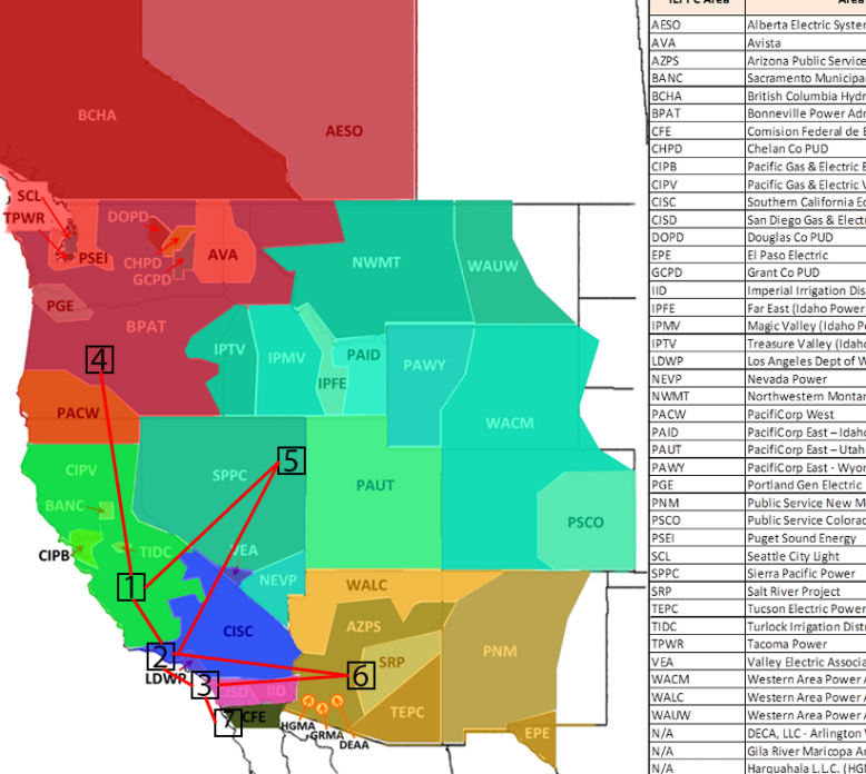
Figure 1: Reduced and modified regions and network for WECC.

The transmission system is simplified to seven regions, as illustrated in Fig. 1, a choice driven by the unavailability of detailed transmission data in the open-source ADS. These regions are delineated based on the topology of the WECC-240. However, regional transmission limitations are still represented using selected lines from the WECC-240 and capacity limits from EIA-930 data, ensuring a realistic portrayal of transmission constraints despite the simplified model. Our approach computed line impedances within the WECC-240 using parallel impedance calculations on manually selected lines, considering only reactance and excluding resistances. This decision aligns with typical practices in market-related studies where transmission line losses are often overlooked. Notably, all impedances were handled in per units (p.u.), ensuring standardization and relevance for our analysis. The capacities for most transmission lines in the WECC-240 are set at a default value of 99,999 MW. To better represent transmission congestion, we set transmission line capacity as the maximum hourly interchange data from neighboring balancing authorities in 2022, sourced from the EIA-930. There are eight transmission lines connecting regions; their parameters are detailed in Table. I.

TABLE I: Transmission Line Parameters

From Region	To Region	Reactance X (p.u.)	Capacity (MW)
1	2	0.0071	6,368
1	4	0.0034	3,500
1	5	0.0299	5,500
2	3	0.0287	888
2	5	0.0195	1,700
2	6	0.0436	3,200
3	6	0.0209	2,200
3	7	0.0270	1,776

III-A2 Generation Resources Data

The information regarding generation resources is entirely sourced from ADS. Since ADS depicts the generation resources projected for 2032, we filtered the data only to include currently existing and in-service generation resources, encompassing 45 coal, 925 natural gas, 6 nuclear, 167 biofuels, 123 geothermal, 669 solar PV units, 351 wind units, 1134 hydropower plants, and 82 energy storage systems. Modeling individual generation units captures the impact of unit commitment and dispatch, which is crucial for realistic market price simulation. Aggregated models often undermine these critical constraints. Therefore, we model individual generation assets in detail in our market simulation model. We compensate for not modeling real-time commitment in CAISO’s procedures for fast-start units by implementing a piece-wise linear cost model for these units in RTD. This model assigns costs varying from $200 to $400 per MW, corresponding to a dispatch capacity range of 0 to 1000 MW.

The total nameplate capacity of thermal generators, which includes geothermal and nuclear resources, stands at 115,320 MW. The total nameplate capacities for wind, solar, hydro, and energy storage are 25,227 MW, 27,002 MW, 66,340 MW, and 16,183 MW, respectively. Table. II compares the installed renewable resources in CAISO from our processed data with the actual figures at the end of 2022 [39]. Notably, the renewable penetration in the table closely aligns with real-world statistics.

TABLE II: Comparison of Test System Renewable Resources with Actual Installations in CAISO (End of 2022)

	Wind	Solar	Hydro	Geo	Bio	Battery
Test System	6,485	16,007	10,077	903	2,583	4,775
Actual	7,950	15,967	12,281	798	1,597	4,614

We model thermal generators using multi-segment piece-wise linear approximated heat rate curves. We directly sourced the maximum/minimum capacity, initial dispatch, segment increment capacity, segment increment heat rate, minimum up/down time, ramp up/down rate, variable operation and maintenance cost, and fuel cost from the ADS. The start-up cost, no-load cost, and segment marginal cost are calculated as detailed below:

$$\mathrm{SUC}_{g} =\mathrm{SUC}_{g}^{fix}+\mathrm{FC}_{g}*\mathrm{SUF}_{g}$$ (1a)

$$\mathrm{NLC}_{g} =\mathrm{FC}_{g}*\mathrm{FMin}_{g}$$ (1b)

$$\mathrm{MC}_{g,gs} =\mathrm{FC}_{g}*\mathrm{HR}_{g,gs}$$ (1c)

where $SUC_{g}$, $NLC_{g}$, and $MC_{g,gs}$ are start-up cost, no-load cost, and segment marginal cost of thermal generator $g$, respectively. $SUC_{g}^{fix}$ is the fixed start-up cost ($), $FC_{g}$ is the fuel cost ($/MMBtu), $SUF_{g}$ is the start-up fuel (MMBtu), $FMin_{g}$ is the minimum fuel input (MMBtu), $HR$ is the linearized heat rate for segment $gs$. To better match real bidding costs during peak loads in our simulation, we increased fuel prices by 20%, mirroring the observed average bidding price rise in generators operating at peak load seasons [19]. It is important to mention that the variable operation and maintenance cost is not incorporated into the segment marginal cost. Instead, it is calculated separately based on the total output, which includes the minimum output.

The ADS provides unit-wise maximum capacity and hourly profiles for wind and solar resources. The 5-min resolution real-time profile generation will be discussed in III-A3. Hourly hydro profiles in the ADS are based on actual generation in 2018. Unlike wind and solar profiles, which are unit-specific, hydro hourly profiles in ADS are summarized by load areas. We employ profiles from the nearest load area as a surrogate for hydropower plants located in areas without specific profiles. Due to data limitation in the public version, we ignore the detailed modeling of water availability and management but model hydroelectric resources’ maximum output does not exceed the maximum hourly output in the hourly profile for each unit, aligning with the ”Hydro-Given Schedule” modeling approach utilized in the ADS production cost model.

For both pumped hydro storage and battery energy storage, only maximum and minimum power capacities is available in the ADS. For pumped hydro storage units lacking pumping capacity data (indicative of positive minimum power capacities) in the ADS, we assigned values as negative maximum power capacities of each unit. The durations for pumped hydro and battery storage are assumed to be 12 hours and 4 hours, respectively. Correspondingly, their one-way efficiencies for charging and discharging are set at 80% and 90%.

III-A3 WECC Load and Renewable Profile

The ADS uses 2018 hourly loads to forecast the loads for 2032, resulting in values higher than current load levels. We normalized the ADS hourly loads to align with current trends to ensure compatibility with test system generation resources. The normalization factor is 0.801, determined from the ratio of CAISO’s DAM load forecast peak/average load to the ADS data for the CAISO area (Regions 1-3). Normalized hourly load profiles for seven regions are used in the DAM simulation.

We incorporated day-ahead forecast errors into the normalized hourly load profiles to create high-temporal-resolution load profiles for RTM simulation. This was achieved using 2022 DAM and RTM load forecast data from CAISO. The CAISO demand forecast for DAM and RTM is organized by Transmission Access Charges (TAC) areas, which do not align perfectly with our delineated Regions 1-3. To address this discrepancy, we mapped CAISO TAC areas to our regions based on geographical alignment: PGE to Region 1; MWD, SCE, and VEA to Region 2; and SDGE to Region 3. The distribution of peak and average load in our assigned regions aligns closely with their corresponding CAISO TAC areas: Region 1 (PGE) has 44%, Region 2 (SCE, MWD, VEA) has 47%, and Region 3 (SDGE) accounts for 9%.

We employed a K-means method to apply historical day-ahead load forecast errors to the ADS hourly load profile. While we opted for this approach, other advanced forecast error generation methodologies could also be utilized. The historical day-ahead prediction error is determined by taking the difference ratio between the DAM and RTM load prediction differences to the DAM load prediction value for each region. The CAISO DAM load forecast data is classified into eight representative days (k=8) based on the hourly total CAISO load and Region 1-3 load. The normalized ADS hourly load profile is then applied to the historical day-ahead load forecast error of the closest representative day. Due to data limitations, RTM load profiles for Regions 4-7, outside CAISO, are derived using a linear regression model trained on DAM and RTM load data from Regions 1-3. This model incorporates 24 distinct features for 24-hour-ahead DAM load predictions, 12 features for 1-hour-ahead RTM load observations, and a feature for the average DAM load per region. For Regions 4-7 prediction, where RTM load observations are unavailable, the series prediction is initiated with day-ahead forecasts, employing a rolling horizon approach based on previously predicted RTM loads. Subsequently, we employ this model in a rolling prediction manner to forecast RTM load in Regions 4-7.

To generate wind and solar profiles for the RTM at a 5-minute resolution, we employ a methodology similar to our approach for load forecasting, utilizing ADS hourly profiles along with CAISO’s historical day-ahead and real-time predictions. Given that CAISO’s historical predictions for wind and solar are based on price hubs rather than specific units, we aggregate ADS wind and solar resources by region for consistency. For Regions 1-3, we implement K-means clustering to create RTM profiles, while for Regions 4-7, we rely on linear regression modeling. Notably, in our solar RTM prediction model, we ensure that the predicted values are set to zero during sunset periods and in instances of negative predictions by post-processing, thus maintaining realism and accuracy in our forecasts. The real-time load and renewable profiles have been refined by scaling the day-ahead forecast errors to match the forecast errors reported by CAISO [40], with a mean absolute percentage error of 1.7% for load, 1.5% for solar, and 6.5% for wind.

III-B Two-Stage Settlement Model

This paper models the wholesale electricity market as a two-stage settlement comprising an hourly-resolution DAM and a high-temporal-resolution RTM. Both can be modeled in look-ahead rolling horizon fashion. In this study, supply-side market participants, encompassing owners of thermal generators, renewable generators, and emerging technologies, submit bids to DAM and RTM. For simplicity, we assume that thermal generators and renewable generators do not exercise market power. Accordingly, they bid at their actual marginal generation cost. Energy storage follows a distinct pricing principle. As a result, we utilize the CAISO 2022 storage hourly average day-ahead and real-time bids by quarter for energy storage bids. Real-time bids are shown in Fig. 2. We assume electricity demand to be inelastic, setting a high value of lost load (VOLL) to avoid infeasibility.

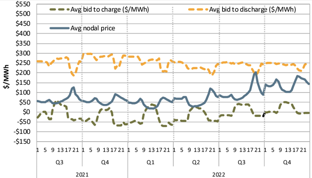
(a) Day-ahead bids.

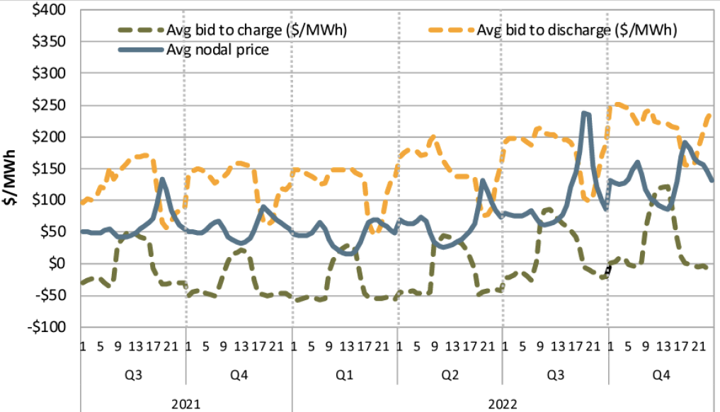
(b) Real-time bids.

Figure 2: CAISO hourly average day-ahead and real-time battery bids and prices by quarter [41].

The market operator conducts a daily DAM to determine next-day unit commitments and schedules the dispatch for each generation of resources with day-ahead load and renewable generation forecast. The objective function of the DAM is to minimize system generation cost, subject to system and generation resources constraints. The constraints of DAM UC include:

• Load balance constraints;

• System-wide operation reserve requirement constraints;

• Transmission line power flow limits;

• Thermal generator total and segment capacity, ramping, minimum up/down time, must run, and state transition constraints;

• Renewable generator availability constraints;

• Energy storage power rating, energy capacity, and state-of-charge evolution constraints.

A more detailed mixed-integer linear program formulation of the DAM UC is given in Appendix--B. Once the DAM UC is solved, the unit commitment outcomes, including hourly on/off statuses and start-up/shutdown decisions, are carried over to the RTM ED. Our test system enables the incorporation of a UC with a look-ahead window beyond the conventional 24-hour UC, aiming to better manage load and renewable fluctuations beyond the immediate operational day.

On the operation day, high-temporal-resolution RTM ED is implemented in a multi-interval rolling horizon setting. With unit commitment binary variables fixed, the RTM ED is modeled as linear programming and illustrated in Appendix -C. With multi-period optimization, only the first time interval decisions will be applied in the real dispatch.

We implement the model in Julia, boasting high computational performance. Annual simulations can be readily executed on a standard personal laptop. The Julia implementation is available on GitHub.

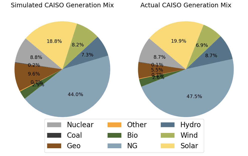
Figure 3: Simulated and 2022 CAISO historical year-long generation mix.

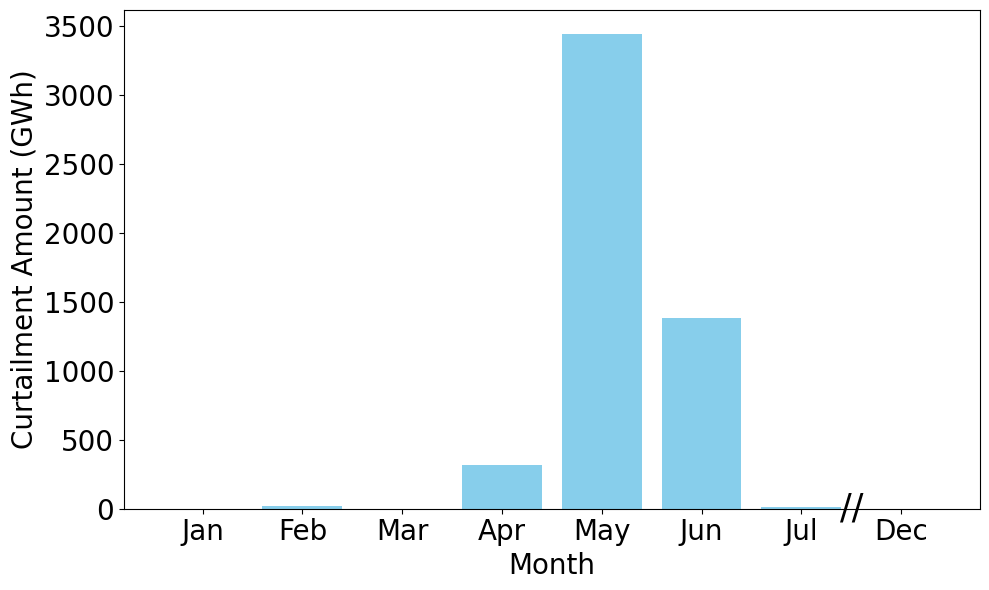
Figure 4: Monthly renewable energy curtailment in GWh: Aug-Nov omitted due to zero curtailment.

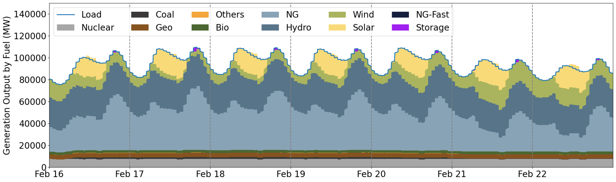
(a) Winter peak week Feb 16-22.

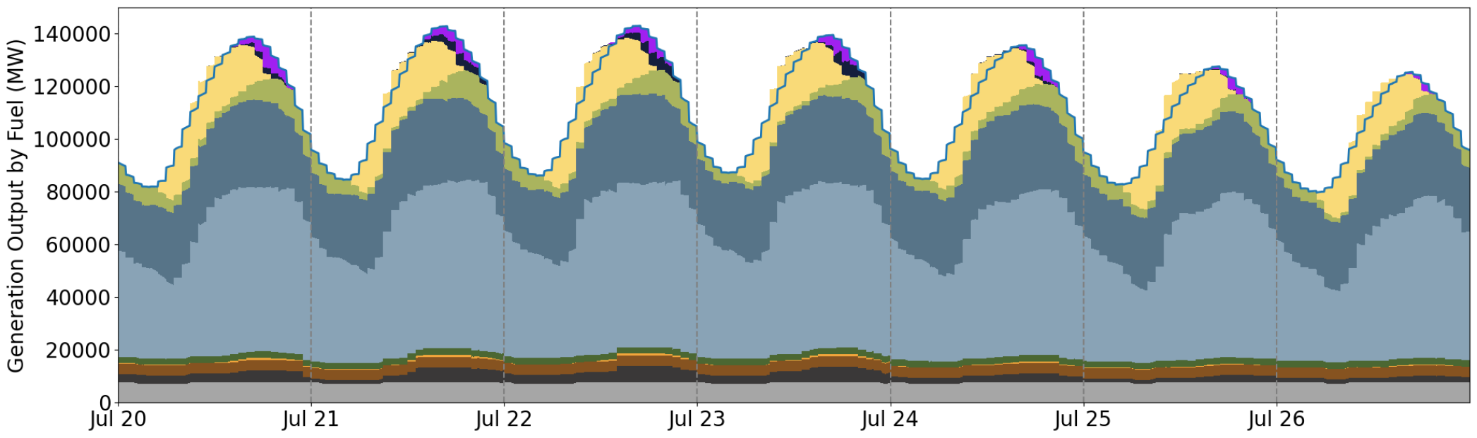
(b) Summer peak week July 20-26.

Figure 5: Total system generation by energy resources during winter and summer peak weeks. Two subfigures shared the same legend.

IV Analysis of Market Simulation Results

We compare the year-long wholesale market simulation results to historical data from CAISO, focusing on generation and price patterns. To ensure sufficient generation capacity for real-time dispatch, we set a 3% operating reserve margin of the hourly predicted load in the DAM UC. Given that we simulate an energy-only market, the VOLL is set at $9000/MWh. We assume that all energy storage units in the system submit identical bids for charging and discharging. These bids are derived from CAISO hourly average bids for the year 2022, as depicted in Fig. 2. Note that although we assume uniform bids in this case study, our test system offers a bidding interface, enabling each energy storage unit to submit strategic bids based on state-of-the-art optimal bidding algorithms. Our year-long simulations use DAM UC without a look-ahead horizon and RTM ED with a thirteen 5-minute interval, amounting to a 65-minute horizon. For multi-interval rolling horizon implementation in DAM and RTM, we consider the solutions of the first 24 intervals (24 hours) in DAM and the first interval (5 minutes) in RTM as the actual cleared results. We also conduct a sensitivity analysis to explore the effects of varying look-ahead horizons in DAM and RTM.

IV-A Generation by Energy Resources

In this subsection, we show the generation pattern observed in our simulation result and compare it with historical statistics from CAISO. As highlighted in the data processing section, the renewable resources capacity in our test system closely mirrors the actual installed capacity in CAISO as of 2022. Fig. 3 compares annual generation mix by energy resources, where the simulated result is from the aggregation of Region 1 to 3, and the actual CAISO data is from California Energy Commission [42]. The simulation generally aligns with the actual generation mix. Fig. 4 highlights the monthly renewable energy curtailment, with notable peaks in spring. This seasonal trend is consistent with CAISO’s typical curtailment patterns, which are influenced by extended daylight hours increasing solar production and seasonal weather changes that increase hydropower availability due to snow melt.

Fig. 5 displays the entire system generation by energy resources in real-time during the winter and summer peak weeks. Generations that exceed load represent energy storage charging power. We see pronounced seasonal patterns in load and renewable generations. Specifically, summer experiences higher loads, with a single peak occurring late afternoon. At the same time, winter sees relatively lower loads and two peaks - one in the morning and another in the evening. Coal power plants are seldom dispatched during winter peak week. However, they are committed to accommodating the overall higher demand in the summer. Both gas turbines and energy storage systems act as flexible resources in peak weeks. They are pivotal in addressing daily load variations and fluctuations within the hour. Energy storage exhibits higher utilization rates in the summer than in winter, often being charged during midday when solar energy peaks and discharged in the late afternoon to meet the surge in energy demand. Fast-start natural gas units are dispatched on the highest peak load days during ramping periods.

IV-B Real-time Price

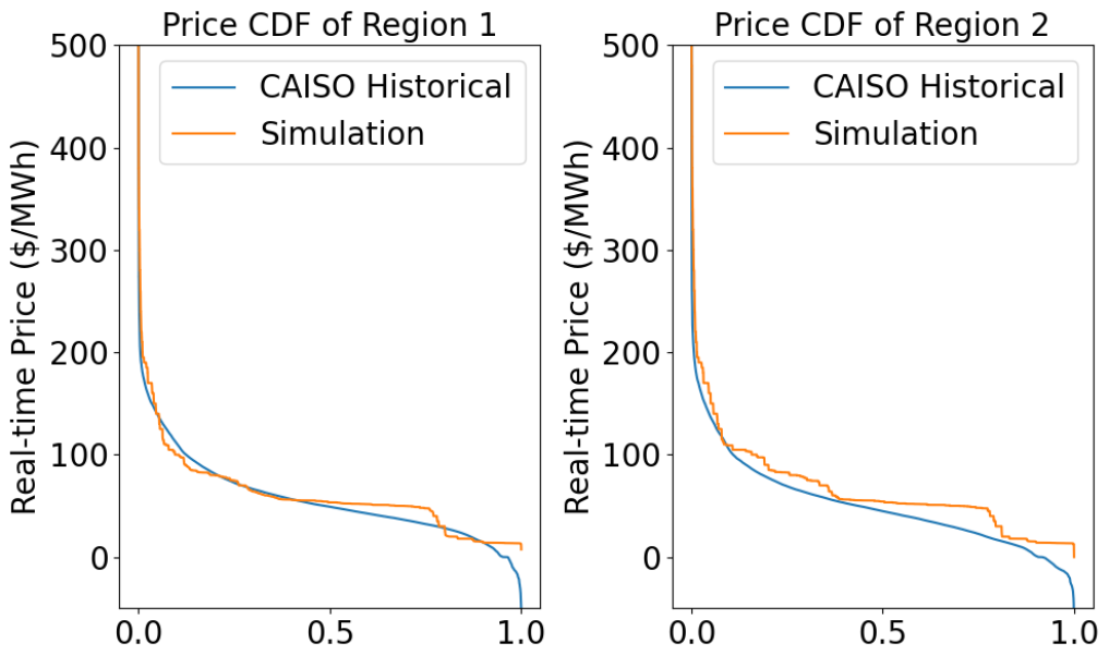
Figure 6: Year-long real-time price cumulative density function comparison.

To further validate our test system, we compare the simulated real-time price patterns to the historical price distribution sourced from CAISO. The geographical locations of Region 1 and 2 is close to CAISO’s price hubs NP15 and SP 15, respectively. Thus, Fig. 6 compares the cumulative distribution function of the year-long simulated real-time prices and the 2022 real-time price data from CAISO hubs. Notably, the simulated real-time price duration curve is similar to historical data. This consistency is crucial, given that emerging technologies, such as energy storage and demand response operations, are sensitive to pricing.

However, there are non-smooth intervals observed within the simulated price duration curves. One reason for this is our assumption that all energy storage units submit identical bids at the hourly average historical bids by quarter. Additionally, we assume thermal generators and renewable resources bid truthfully at their marginal cost. We also notice short right tails in the simulation result, which indicates less low prices. Due to data limitations, our test system uses a reduced seven regions instead of an actual comprehensive network. This simplification leads to less congestion, which is one of the most common factors for negative prices within CAISO.

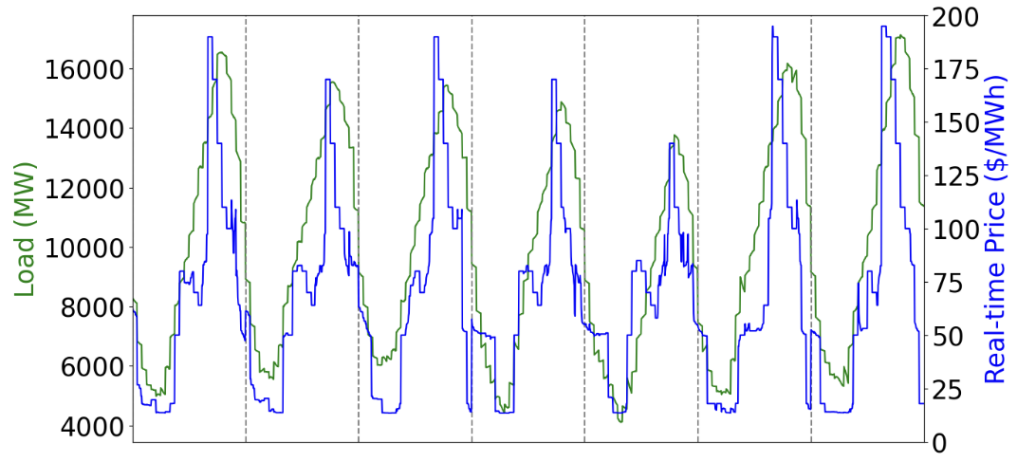
(a) 1 week example.

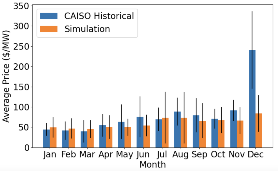
(b) Monthly statistics.

Figure 7: Example of simulated real-time price. (a) 1 week real-time price and load; (b) monthly statistics compared to CAISO historical data.

Fig. 7(a) offers a snapshot of the real-time load and price over a week. We observe low prices in mid of the day and price surges during ramping-up periods. Figure 7(b) displays a month-by-month comparison of average real-time prices between CAISO historical data and market simulation model results, with error bars representing plus/minus one standard deviation. The patterns align closely for most of the year, indicating a strong correlation in monthly price trends. However, notable deviations emerge in November and December, where the simulated prices are significantly lower than historical prices. This divergence is attributed to an anomalous spike in natural gas prices from late November 2022 through January 2023, which is not captured by the simulation model [43].

IV-C Sensitivity Analysis

To effectively manage the multi-day and intra-hour uncertainties of renewable generation and the state-of-charge in energy storage systems, certain system operators have adopted look-ahead windows with a rolling horizon in DAM and RTM. We conduct a year-long simulation incorporating different ED and UC optimization horizons. The aim is to examine the impact of look-ahead horizons on ED and UC outcomes.

We assessed the influence of the ED look-ahead horizon by considering scenarios with no look-ahead UC. ED look-ahead horizon across 1, 6, and 13 five-minute intervals. The single interval aligns with conventional ED practices, while the 13-interval approach corresponds with current CAISO real-time market regulations. Incorporating ED look-ahead into the model, we found that 6 and 13 five-minute intervals reduced system costs by 0.04% and 0.12%, respectively, offering improved predictions of intra-hour load and renewable fluctuations. We also explored the effect of the UC look-ahead horizon, comparing cases without ED look-ahead, including UC with 24, 48, and 72-hour horizons. Integrating UC look-ahead into the model yields negligible cost reductions, as the benefit of longer UC look-ahead periods for slow ramping generators’ commitment is counterbalanced by the presence of relatively low-cost, fast-response generation units in the real-time dispatch. It is also worth noting that these cost-saving estimations are likely lower than in practice, as our proposed model does not consider contingency scenarios or planned generator outages.

V Conclusion

This study set a robust foundation for wholesale market simulation, designed to support detailed electricity market analysis, enabling a finer time granularity crucial for thoroughly examining real-time market designs and integrating emerging alternative energy resources. Our model is initially tailored to CAISO and reflects its advanced renewable energy and storage integration. Our versatile model can be adapted in other ISOs/RTOs with two-settlement clearing markets. It requires data on generation resources, time-coincident day-ahead and real-time load, renewable profiles, and network topology, particularly suited for markets with a two-stage settlement process. Our constructed WECC-based simulation closely mirrors the generation and pricing dynamics of CAISO and underscores the potential of price-sensitive resources. As we look ahead to future research, integrating state-of-the-art strategic bidding algorithms for emerging technologies emerges as a promising avenue. Furthermore, incorporating a more detailed network topology will bolster the fidelity and applicability of our model. Ultimately, this framework provides a foundation for exploring innovative market rules and designs, especially when intertwined with the capabilities of emerging technologies.

-A Nomenclature

-A1 Sets and Indices

$Z$

Set of regions, indexed by $z$

$G,G_{z},G_{m}$

Set of thermal generators, subset of thermal generators in region $z$, and subset of must-run generators, indexed by $g$

$GS_{g}$

Set of segments of thermal generator $g$, indexed by $gs$

$GR,GR_{z}$

Set of renewable generators and subset of renewable generators in region $z$, indexed by $gr$

$S,S_{z}$

Set of energy storage and subset of energy storage in region $z$, indexed by $s$

$L,LT_{z},LF_{z}$

Set of transmission lines and subset of transmission line to/from region $z$, indexed by $l$

$H$

Set of hours for DAM, indexed by $h$

$T$

Set of time intervals for RTM, indexed by $t$

-A2 Variables

$gt_{g,h}$

Thermal generator output power, MW

$gts_{g,gs,h}$

Thermal generator segment output power, MW

$r_{g,h}$

Ramping product by thermal generator, MW

$u_{g,h}$

Thermal generator commitment status, binary

$v_{g,h},w_{g,h}$

Thermal generator start-up/shut-down decision, binary

$gr_{g,h}$

Renewable generator output power, MW

$d_{s,h},c_{s,h}$

Energy storage energy discharge/charge power, MW

$f_{l,h}$

Line power flow, MW

$\theta_{z,t}$

Voltage phase angle

$s_{z,h}$

unserved energy, MW

-A3 Parameters

$\mathrm{MC}_{g,gs}$

Generator segment marginal fuel cost, $/MW

$\mathrm{VOM}_{g}$

Generator variable operations and maintenance cost, $/MW

$\mathrm{NLC}_{g}$

Generator no-load cost, $

$\mathrm{SUC}_{g}$

Generator start-up cost, $

$\mathrm{P}^{max}_{g},\mathrm{P}^{min}_{g}$

Generator maximum and minimum power output, MW

$\mathrm{PS}^{max}_{g,gs}$

Generator segment maximum power output, MW

$\mathrm{RU}_{g},\mathrm{RU}_{g}$

Generator maximum ramp up/down rate, MW/hour

$\mathrm{UT}_{g},\mathrm{DT}_{g}$

Generator minimum up/down time, hour

$\mathrm{SU}_{g},\mathrm{SD}_{g}$

Number of hours generator must stay up/down since the start of the optimization horizon, hour

$\mathrm{RA}_{gr,h}$

Renewable maximum expected capacity, MW

$\mathrm{D}^{max}_{s},\mathrm{D}^{min}_{s}$

Energy storage maximum and minimum discharge power rating, MW

$\mathrm{C}^{max}_{s},\mathrm{C}^{min}_{s}$

Energy storage maximum and minimum charge power rating, MW

$\mathrm{\eta}^{D}_{s},\mathrm{\eta}^{C}_{s}$

Energy storage discharge and charge efficiency

$\mathrm{E}^{max}_{s},\mathrm{E}^{min}_{s}$

Energy storage maximum and minimum energy capacity, MWh

$\mathrm{E}^{T}_{s}$

Energy storage targeted state-of-charge at end of the operation day, MWh

$\mathrm{B}^{D}_{s},\mathrm{B}^{C}_{s}$

Energy storage discharge and charge bids, $/MW

$\mathrm{F}^{max}_{l},\mathrm{F}^{min}_{l}$

Transmission line maximum and minimum power flow, MW

$T(l),F(l)$

Transmission line $l$ to and from zone

$\mathrm{X}_{l}$

Transmission line reactance, p.u.

$\mathrm{L}_{z,h}$

Inflexible load, MW

$\mathrm{RM}$

Opearation reserve marging

$\mathrm{VOLL}$

Value of loss load, $/MW

$\mathrm{SC}$

Time scaling constant for RTM

-B DAM UC Formulation

The objective of the DAM UC is to minimize the total system cost for the upcoming operational day. When incorporating a look-ahead horizon into the model, the optimization aims to minimize costs over the entire optimization period. This look-ahead feature allows the model to consider not just the immediate next day but also subsequent periods, providing a more holistic approach to system operation by anticipating future events and making decisions accordingly.

$$\begin{gathered}min\sum_{h}^{H}\Bigl{[}\sum_{g\in G}\Bigl{(}\sum_{gs\in GS}({\mathrm{MC}_{g,gs}*gts_{g,gs,h})}\\ +VOM_{g}*gt_{g,h}+\mathrm{NLC}_{g}*u_{g,h}+\mathrm{SUC}_{g}*v_{g,h}\Bigl{)}\\ \sum_{s}^{S}\Bigl{(}\mathrm{B}^{D}_{s,h}*d_{s,h}-\mathrm{B}^{C}_{s,h}*c_{s,h}\Bigl{)}+\sum_{z}^{Z}\mathrm{VOLL}*s_{z,h}\Bigl{]}\end{gathered}$$ (2d)

-B1 System Level Constraints

$$\sum_{g\in G_{z}}gt_{g,h} +\sum_{gr\in GR_{z}}gr_{gr,h}+\sum_{s\in S_{z}}\left(d_{s,h}-c_{s,h}\right)$$

$$+\sum_{l\in LT_{z}}f_{l,h} -\sum_{l\in LF_{z}}f_{l,h}+s_{z,h}=\mathrm{L}_{z,h}$$ (2e)

$$\sum_{g\in G} r_{g,h}\geq\mathrm{RM}\cdot\sum_{z\in Z}\mathrm{L}_{z,h}$$ (2f)

System level constraints include load balance (2e) and system operation reserve requirement (2f). The operation reserve requirement in our model is for whole system and each hour, proportional to the hourly load forecast.

-B2 Transmission Constraints

$$\mathrm{F}^{min}_{l} \leq f_{l,h}\leq\mathrm{F}^{max}_{l}$$ (2g)

$$f_{l,h} =\mathrm{X}_{l}*(\theta_{T(l),h}-\theta_{F(l),h})$$ (2h)

$$\theta_{ref,h} =0$$ (2i)

We model transmission using DC-OPF. (2g) models the transmission capacity. (2h) and (2i) models the voltage phase angle, where $F(l)$, $T(l)$ are from region and to region of line $l$. $ref$ is the reference region.

-B3 Thermal Generator Constraints

$$gt_{g,h} =\mathrm{P}^{min}_{g}*u_{g,h}+\sum_{g\in G}gts_{g,gs,h}$$ (2j)

$$\mathrm{P}^{min}_{g}*u_{g,h} \leq gt_{g,h}\leq\mathrm{P}^{max}_{g}*u_{g,h}$$ (2k)

$$0 \leq gts_{g,gs,h}\leq\mathrm{PS}^{max}_{g,gs}$$ (2l)

$$-gt_{g,h}+gt_{g,h-1} \leq\mathrm{RD}_{g}+\mathrm{P}^{min}_{g}*w_{g,h}$$ (2m)

$$gt_{g,h}-gt_{g,h-1} \leq\mathrm{RU}_{g}+\mathrm{P}^{min}_{g}*v_{g,h}$$ (2n)

$$r_{g,h} \leq\mathrm{P}^{max}_{g}\cdot u_{g,h}-gt_{g,h}$$ (2o)

$$r_{g,h} \leq\mathrm{RU}_{g}$$ (2p)

$$u_{g,h} =1,\quad\forall g\in G_{m}$$ (2q)

$$v_{g,h}-w_{g,h} =u_{g,h}-u_{g,h-1}$$ (2r)

$$v_{g,h}+w_{g,h} \leq 1$$ (2s)

$$\sum_{\tau=\max\{h-\mathrm{UT}_{g}+1,1\}}^{h}v_{g,\tau} \leq u_{g,h},h\in\{\mathrm{SU}_{g},\dotsc,H\}$$ (2t)

$$\sum_{\tau=\max\{h-\mathrm{DT}_{g}+1,1\}}^{h}w_{g,\tau} \leq 1-u_{g,h},h\in\{\mathrm{SD}_{g},\dotsc H\}$$ (2u)

(2j), (2k), and (2l) models the total output and segment output of a thermal generator. (2m) and (2n) are ramp-up and ramp-down constraints. At the beginning of optimization horizon, $gt_{g,h-1}$ in (2m) and (2n) are parameters representing initial output. (2o) and (2p) limit the ability of generators providing operation ramping products. (2q) is the must-run constraints. (2r)–(2u) are state transition and must up and down time constraints. With a rolling horizon, the remaining minimum up and down time at the end of operation day will be passed to next DAM UC.

-B4 Renewable Generator Availability Constraints

$$0\leq gr_{gr,h}\leq\mathrm{RA}_{gr,h}$$ (2v)

Due to the limitation of the hydro power system data, hydro resources are similarly modeled as solar and wind resources. The maximum generation from each renewable generation unit may not exceed the maximum expected capacity.

-B5 Energy Storage Constraints

$$\mathrm{D}^{min}_{s} \leq d_{s,h}\leq\mathrm{D}^{max}_{s}$$ (2w)

$$\mathrm{C}^{min}_{s} \leq c_{s,h}\leq\mathrm{C}^{max}_{s}$$ (2x)

$$e_{s,h}-e_{s,h-1} =\mathrm{\eta}^{C}_{s}*c_{s,h}-\frac{1}{\mathrm{\eta}^{D}_{s}}*d_{s,h}$$ (2y)

$$\mathrm{E}^{min}_{s} \leq e_{s,h}\leq\mathrm{E}^{max}_{s}$$ (2z)

$$e_{s,t}\geq E^{T}_{s}, \quad\forall\{t\in T\mid t\equiv 0\ (\text{mod}\ 24)\}$$ (2aa)

Constraints for energy storage systems include discharge and charge power capacity (2w),(2x), state-of-charge evolution (2y), and energy capacity (2z). At the begining of optimization horizon, $e_{t-1}$ in (2y) is a parameter representing initial state-of-charge. The targeted state-of-charge is defined by (2aa).

-C RTM ED Formulation

In the context of a rolling-horizon with a look-ahead window, the RTM ED borrows certain similarities from the DAM UC formulation. In the DAM UC, unit commitment decisions are made using binary variables $u_{g,h}$, $v_{g,h}$, and $w_{g,h}$. These decisions, when transitioned to the RTM ED context, transform into parameters, denoted as $U_{g,t}$, $V_{g,t}$, and $W_{g,t}$. Here’s a breakdown of their correspondence:

• $U_{g,t}$ in the RTM ED represents whether a unit is committed during a particular hour. It will be set to 1 if its corresponding hour variable $u_{g,h}$ is 1.

• $V_{g,t}$ in the RTM ED indicates the start-up decision of a unit at the beginning of an hour interval. It will be set to 1 only if $t$ is interval at beginning of an operation hour and $v_{g,h}$ in the DAM UC for that hour is 1.

• $W_{g,t}$ in the RTM ED indicates the shut-down decision of a unit at the beginning of an hour interval. It will be set to 1 only if $t$ is interval at beginning of an operation hour and $w_{g,h}$ in the DAM UC for that hour is 1.

The objective function of RTM ED is

$$\begin{gathered}\min\quad SC*\sum_{t}^{T}\Bigl{[}\sum_{g\in G}\Bigl{(}\sum_{gs\in GS}({\mathrm{MC}_{g,gs}*gts_{g,gs,t})}\\ +VOM_{g}*gt_{g,t}+\mathrm{NLC}_{g}*U_{g,t}+\mathrm{SUC}_{g}*V_{g,t}\Bigl{)}\\ \sum_{s}^{S}\Bigl{(}\mathrm{B}^{D}_{s,t}*d_{s,t}-\mathrm{B}^{C}_{s,t}*c_{s,t}\Bigl{)}+\sum_{z}^{Z}\mathrm{VOLL}*s_{z,t}\Bigl{]}\end{gathered}$$ (3d)

Subject to constraints include load balance constraint (2e), transmission constraints (2g)–(2i), thermal generator constraints (2j)–(2n), renewable availability constraint (2v), and energy storage constraints (2w)–(2z). All variables with time interval indexed by $h$ are replaced with shorter interval indexed $t$.

Note that energy storage state-of-charge evolution constraint (2y) and ramping constraints (2m),(2n) are scaled by time scaling constant $\mathrm{SC}$:

$$e_{s,t}-e_{s,t-1} =\mathrm{SC}*(\mathrm{\eta}^{C}_{s}*c_{s,t}-\frac{1}{\mathrm{\eta}^{D}_{s}}*d_{s,t})$$ (3e)

$$-gt_{g,t}+gt_{g,t-1} \leq\mathrm{SC}*\mathrm{RD}_{g}+\mathrm{P}^{min}_{g}*W_{g,t}$$ (3f)

$$gt_{g,t}-gt_{g,t-1} \leq\mathrm{SC}*\mathrm{RU}_{g}+\mathrm{P}^{min}_{g}*V_{g,t}$$ (3g)

References

- [1] Congressional Budget Office, “Emissions of carbon dioxide in the electric power sector,” DEC 2022. [Online]. Available: https://www.cbo.gov/publication/58419
- [2] National Conference of State Legislatures, “State renewable portfolio standards and goals,” Augest 2022. [Online]. Available: https://www.ncsl.org/energy/state-renewable-portfolio-standards-and-goals
- [3] Potomac Economics, “2022 state of the market report for the ercot electricity markets,” pp. 30–32, 2023.
- [4] California ISO, “Key statistics,” July 2023. [Online]. Available: http://www.caiso.com/Documents/Key-Statistics-July-2023.pdf
- [5] ——, “20-year transmission outlook,” May 2022. [Online]. Available: http://www.caiso.com/InitiativeDocuments/20-YearTransmissionOutlook-May2022.pdf
- [6] R. Morrison, “Energy system modeling: Public transparency, scientific reproducibility, and open development,” Energy Strategy Reviews, vol. 20, pp. 49–63, 2018.
- [7] D. Wu, X. Zheng, Y. Xu, D. Olsen, B. Xia, C. Singh, and L. Xie, “An open-source extendable model and corrective measure assessment of the 2021 texas power outage,” Advances in Applied Energy, vol. 4, p. 100056, 2021.
- [8] L. Xie, P. M. Carvalho, L. A. Ferreira, J. Liu, B. H. Krogh, N. Popli, and M. D. Ilić, “Wind integration in power systems: Operational challenges and possible solutions,” Proceedings of the IEEE, vol. 99, no. 1, pp. 214–232, 2010.
- [9] H. Shaker, H. Zareipour, and D. Wood, “Impacts of large-scale wind and solar power integration on california’s net electrical load,” Renewable and Sustainable Energy Reviews, vol. 58, pp. 761–774, 2016.
- [10] J. Wang, J. Mao, R. Hao, S. Li, and G. Bao, “Multi-energy coupling analysis and optimal scheduling of regional integrated energy system,” Energy, vol. 254, p. 124482, 2022.
- [11] B. Xu, Y. Wang, Y. Dvorkin, R. Fernández-Blanco, C. A. Silva-Monroy, J.-P. Watson, and D. S. Kirschen, “Scalable planning for energy storage in energy and reserve markets,” IEEE Transactions on Power systems, vol. 32, no. 6, pp. 4515–4527, 2017.
- [12] F. Oldewurtel, T. Borsche, M. Bucher, P. Fortenbacher, M. G. V. T. Haring, T. Haring, J. L. Mathieu, O. Mégel, E. Vrettos, and G. Andersson, “A framework for and assessment of demand response and energy storage in power systems,” in 2013 IREP Symposium Bulk Power System Dynamics and Control-IX Optimization, Security and Control of the Emerging Power Grid. IEEE, 2013, pp. 1–24.
- [13] K. Sun, K.-J. Li, Z. Zhang, Y. Liang, Z. Liu, and W.-J. Lee, “An integration scheme of renewable energies, hydrogen plant, and logistics center in the suburban power grid,” IEEE Transactions on Industry Applications, vol. 58, no. 2, pp. 2771–2779, 2021.
- [14] Z. Ji, C. Kang, Q. Chen, Q. Xia, C. Jiang, Z. Chen, and J. Xin, “Low-carbon power system dispatch incorporating carbon capture power plants,” IEEE Transactions on power systems, vol. 28, no. 4, pp. 4615–4623, 2013.
- [15] R. Christie and I. Dabbagchi, “Uw power system test case archive,” 1999. [Online]. Available: https://labs.ece.uw.edu/pstca/
- [16] V. Dvorkin and A. Botterud, “Differentially private algorithms for synthetic power system datasets,” IEEE Control Systems Letters, vol. 7, pp. 2053–2058, 2023.
- [17] H. Yuan, R. S. Biswas, J. Tan, and Y. Zhang, “Developing a reduced 240-bus wecc dynamic model for frequency response study of high renewable integration,” in 2020 IEEE/PES Transmission and Distribution Conference and Exposition (T&D), 2020, pp. 1–5.
- [18] J. E. Price and J. Goodin, “Reduced network modeling of wecc as a market design prototype,” in 2011 IEEE Power and Energy Society General Meeting. IEEE, 2011, pp. 1–6.
- [19] M. V. Liu, B. Yuan, Z. Wang, J. A. Sward, K. M. Zhang, and C. L. Anderson, “An Open Source Representation for the NYS Electric Grid to Support Power Grid and Market Transition Studies,” IEEE Transactions on Power Systems, pp. 1–11, 2022.
- [20] S. Taylor, A. Rangarajan, N. Rhodes, J. Snodgrass, B. Lesieutre, and L. A. Roald, “California Test System (CATS): A Geographically Accurate Test System based on the California Grid,” Jun. 2023, arXiv:2210.04351 [cs, eess]. [Online]. Available: http://arxiv.org/abs/2210.04351
- [21] D. Krishnamurthy, W. Li, and L. Tesfatsion, “An 8-zone test system based on iso new england data: Development and application,” IEEE Transactions on Power Systems, vol. 31, no. 1, pp. 234–246, 2015.
- [22] S. Battula, L. Tesfatsion, and T. E. McDermott, “An ERCOT test system for market design studies,” Applied Energy, vol. 275, p. 115182, Oct. 2020.
- [23] S. Wang, N. Zheng, C. D. Bothwell, Q. Xu, S. Kasina, and B. F. Hobbs, “Crediting variable renewable energy and energy storage in capacity markets: Effects of unit commitment and storage operation,” IEEE Transactions on Power Systems, vol. 37, no. 1, pp. 617–628, 2022.
- [24] T. Levin, J. Bistline, R. Sioshansi, W. J. Cole, J. Kwon, S. P. Burger, G. W. Crabtree, J. D. Jenkins, R. O’Neil, M. Korpås et al., “Energy storage solutions to decarbonize electricity through enhanced capacity expansion modelling,” Nature Energy, pp. 1–10, 2023.
- [25] T. Qiu, B. Xu, Y. Wang, Y. Dvorkin, and D. S. Kirschen, “Stochastic multistage coplanning of transmission expansion and energy storage,” IEEE Transactions on Power Systems, vol. 32, no. 1, pp. 643–651, 2017.
- [26] H. Gómez-Villarreal, M. Cañas Carretón, R. Zárate-Miñano, and M. Carrión, “Generation capacity expansion considering hydrogen power plants and energy storage systems,” IEEE Access, vol. 11, pp. 15 525–15 539, 2023.
- [27] R. Van Haaren, M. Morjaria, and V. Fthenakis, “Empirical assessment of short-term variability from utility-scale solar pv plants,” Progress in Photovoltaics: Research and Applications, vol. 22, no. 5, pp. 548–559, 2014.
- [28] Y.-K. Wu, C.-R. Chen, and H. Abdul Rahman, “A novel hybrid model for short-term forecasting in pv power generation,” International Journal of Photoenergy, vol. 2014, pp. 1–9, 2014.
- [29] E. Ela, V. Diakov, E. Ibanez, and M. Heaney, “Impacts of variability and uncertainty in solar photovoltaic generation at multiple timescales,” National Renewable Energy Lab.(NREL), Golden, CO (United States), Tech. Rep., 2013.
- [30] B. Sergi, C. Feng, F. Zhang, B.-M. Hodge, R. Ring-Jarvi, R. Bryce, K. Doubleday, M. Rose, G. Buster, and M. Rossol, “Arpa-e perform datasets,” DOE Open Energy Data Initiative (OEDI); National Renewable Energy Laboratory …, Tech. Rep., 2022.
- [31] H. A. Aalami and S. Nojavan, “Energy storage system and demand response program effects on stochastic energy procurement of large consumers considering renewable generation,” IET Generation, Transmission & Distribution, vol. 10, no. 1, pp. 107–114, 2016.
- [32] B. Xu, J. Zhao, T. Zheng, E. Litvinov, and D. S. Kirschen, “Factoring the cycle aging cost of batteries participating in electricity markets,” IEEE Transactions on Power Systems, vol. 33, no. 2, pp. 2248–2259, 2017.
- [33] K.-W. Cheng, Y. Bian, Y. Shi, and Y. Chen, “Carbon-aware ev charging,” in 2022 IEEE International Conference on Communications, Control, and Computing Technologies for Smart Grids (SmartGridComm), 2022, pp. 186–192.
- [34] R. W. Howarth and M. Z. Jacobson, “How green is blue hydrogen?” Energy Science & Engineering, vol. 9, no. 10, pp. 1676–1687, 2021.
- [35] C. Yang, Z. Cong, D. Guibo, L. Yicheng, Y. Shipeng, and S. Zhuo, “Multi objective low carbon economic dispatch of power system considering integrated flexible operation of carbon capture power plant,” in 2021 Power System and Green Energy Conference (PSGEC). IEEE, 2021, pp. 321–326.
- [36] A. Menati, X. Zheng, K. Lee, R. Shi, P. Du, C. Singh, and L. Xie, “High resolution modeling and analysis of cryptocurrency mining’s impact on power grids: Carbon footprint, reliability, and electricity price,” Advances in Applied Energy, vol. 10, p. 100136, 2023.
- [37] N. Zheng, X. Qin, D. Wu, G. Murtaugh, and B. Xu, “Energy storage state-of-charge market model,” IEEE Transactions on Energy Markets, Policy and Regulation, vol. 1, no. 1, pp. 11–22, 2023.
- [38] J. Jalving, J. Ghouse, N. Cortes, X. Gao, B. Knueven, D. Agi, S. Martin, X. Chen, D. Guittet, R. Tumbalam-Gooty et al., “Beyond price taker: conceptual design and optimization of integrated energy systems using machine learning market surrogates,” Applied Energy, vol. 351, p. 121767, 2023.
- [39] California ISO, “Key statistics,” Dec 2022. [Online]. Available: http://www.caiso.com/Documents/Key-Statistics-Dec-2022.pdf
- [40] ——, “Market performance planning forum - dec 14, 202212/14/2022 15:12,” Dec 2022. [Online]. Available: http://www.caiso.com/Documents/Presentation-MarketPerformancePlanningForum-Dec14-2022.pdf
- [41] ——, “Special report on battery storage,” July 2023. [Online]. Available: http://www.caiso.com/Documents/2022-Special-Report-on-Battery-Storage-Jul-7-2023.pdf
- [42] California Energy Commission, “2022 total system electric generation,” 2023. [Online]. Available: https://www.energy.ca.gov/data-reports/energy-almanac/california-electricity-data/2022-total-system-electric-generation
- [43] California ISO, “Special report on gas conditions and caiso markets,” Feb 2023. [Online]. Available: http://www.caiso.com/Documents/special-report-on-gas-conditions-and-caiso-markets-for-december-2022-and-january-2023-published.html